The Entire Regularization Path for the Support …jmlr.csail.mit.edu/papers/volume5/hastie04a/hastie04a.pdf · The Entire Regularization Path for the Support Vector Machine ... (Hastie

Journal of Machine Learning Research 5 (2004) 1391–1415 Submitted 3/04; Published 10/04

The Entire Regularization Path for the Support Vector Machine

Trevor Hastie [email protected]

Department of StatisticsStanford UniversityStanford, CA 94305, USA

Saharon Rosset [email protected] .COM

IBM Watson Research CenterP.O. Box 218Yorktown Heights, NY 10598, USA

Robert Tibshirani [email protected]

Department of StatisticsStanford UniversityStanford, CA 94305, USA

Ji Zhu JIZHU@UMICH .EDU

Department of StatisticsUniversity of Michigan439 West Hall550 East UniversityAnn Arbor, MI 48109-1092, USA

Editor: Nello Cristianini

Abstract

The support vector machine (SVM) is a widely used tool for classification. Many efficient imple-mentations exist for fitting a two-class SVM model. The user has to supply values for the tuningparameters: the regularization cost parameter, and the kernel parameters. It seems a common prac-tice is to use a default value for the cost parameter, often leading to the least restrictive model.In this paper we argue that the choice of the cost parameter can be critical. We then derive analgorithm that can fit the entire path of SVM solutions for every value of the cost parameter, withessentially the same computational cost as fitting one SVM model. We illustrate our algorithm onsome examples, and use our representation to give further insight into the range of SVM solutions.

Keywords: support vector machines, regularization, coefficient path

1. Introduction

In this paper we study the support vector machine (SVM)(Vapnik, 1996;Scholkopf and Smola,2001) for two-class classification. We have a set ofn training pairsxi ,yi , wherexi ∈R

p is ap-vectorof real-valued predictors (attributes) for theith observation, andyi ∈ {−1,+1} codes its binaryresponse. We start off with the simple case of a linear classifier, where our goal is to estimate alinear decision function

f (x) = β0 +βTx, (1)

c©2004 Trevor Hastie, Saharon Rosset, Robert Tibshirani and Ji Zhu.

HASTIE, ROSSET, TIBSHIRANI AND ZHU

−0.5 0.0 0.5 1.0 1.5 2.0

−1.

0−

0.5

0.0

0.5

1.0

1.5

7

8

9

10

11

12

1

2

3

4

5

6

1/||β||f (x) = 0

f (x) = +1

f (x) = −1

Figure 1: A simple example shows the elements of a SVM model. The “+1” points are solid,the “-1” hollow. C = 2, and the width of the soft margin is 2/||β|| = 2× 0.587. Twohollow points{3,5} are misclassified, while the two solid points{10,12} are correctlyclassified, but on the wrong side of their marginf (x) = +1; each of these hasξi > 0. Thethree square shaped points{2,6,7} are exactly on the margin.

and its associated classifierClass(x) = sign[ f (x)]. (2)

There are many ways to fit such a linear classifier, including linear regression, Fisher’s lineardiscriminant analysis, and logistic regression (Hastie et al., 2001, Chapter4). If the training dataare linearly separable, an appealing approach is to ask for the decision boundary{x : f (x) = 0}that maximizes the margin between the two classes (Vapnik, 1996). Solving such a problem is anexercise in convex optimization; the popular setup is

minβ0,β

12||β||2 subject to, for each i:yi(β0 +xT

i β) ≥ 1. (3)

A bit of linear algebra shows that1||β||(β0 + xTi β) is the signed distance fromxi to the decision

boundary. When the data are not separable, this criterion is modified to

minβ0,β

12||β||2 +C

n

∑i=1

ξi , (4)

subject to, for eachi: yi(β0 +xTi β) ≥ 1−ξi .

1392

SVM REGULARIZATION PATH

-3 -2 -1 0 1 2 3

0.0

0.5

1.0

1.5

2.0

2.5

3.0

Binomial Log-likelihoodSupport Vector

y f(x)

Loss

Figure 2: The hinge loss penalizes observation marginsy f(x) less than+1 linearly, and is indiffer-ent to margins greater than+1. The negative binomial log-likelihood (deviance) has thesame asymptotes, but operates in a smoother fashion near theelbowaty f(x) = 1.

Here theξi are non-negative slack variables that allow points to be on the wrong side of their “softmargin” (f (x) = ±1), as well as the decision boundary, andC is a cost parameter that controls theamount of overlap. Figure 1 shows a simple example. If the data are separable, then for sufficientlylargeC the solutions to (3) and (4) coincide. If the data are not separable, asC gets large thesolution approaches the minimum overlap solution with largest margin, which is attained for somefinite value ofC.

Alternatively, we can formulate the problem using aLoss+ Penaltycriterion (Wahba et al.,2000; Hastie et al., 2001):

minβ0,β

n

∑i=1

[1−yi(β0 +βTxi)]+ +λ2||β||2. (5)

The regularization parameterλ in (5) corresponds to 1/C, with C in (4). Here thehinge lossL(y, f (x)) = [1− y f(x)]+ can be compared to the negative binomial log-likelihoodL(y, f (x)) =log[1+exp(−y f(x))] for estimating the linear functionf (x) = β0 +βTx; see Figure 2.

This formulation emphasizes the role of regularization. In many situations we have sufficientvariables (e.g. gene expression arrays) to guarantee separation. Wemay nevertheless avoid themaximum margin separator (λ ↓ 0), which is governed by observations on the boundary, in favor ofa more regularized solution involving more observations.

This formulation also admits a class of more flexible, nonlinear generalizations

minf∈H

n

∑i=1

L(yi , f (xi))+λJ( f ), (6)

where f (x) is an arbitrary function in some Hilbert spaceH , andJ( f ) is a functional that measuresthe “roughness” off in H .

The nonlinearkernelSVMs arise naturally in this context. In this casef (x) = β0 + g(x), andJ( f ) = J(g) is a norm in a Reproducing Kernel Hilbert Space of functionsHK generated by a

1393


oo

ooo

o

o

o

o

o

o

o

o

oo

o

o o

o

o

o

o

o

o

o

o

o

o

o

o

o

o

oo

o

o

o

o

o

o

o

o

o

o

o

o

o

o

o

o

o

o

o

o

o

o

o

o

oo

o

o

o

o

o

o

o

o

o

oo o

oo

oo

o

oo

o

o

o

oo

o

o

o

o

o

o

o

o

o

o

o

o

oo

o

o

o

oo

o

o

o

o

o

o

o

o

o

o

o

o

o

o

oo

o

o

o

o

o

o

o

o ooo

o

o

ooo o

o

o

o

o

o

o

o

oo

o

o

oo

ooo

o

o

ooo

o

o

o

o

o

o

o

oo

o

o

o

o

o

o

oo

ooo

o

o

o

o

o

o

oo

oo

oo

o

o

o

o

o

o

o

o

o

o

o

Training Error: 0.160

Test Error: 0.218Bayes Error: 0.210

Radial Kernel:C = 2, γ = 1

oo

ooo

o

o

o

o

o

o

o

o

oo

o

o o

o

o

o

o

o

o

o

o

o

o

o

o

o

o

oo

o

o

o

o

o

o

o

o

o

o

o

o

o

o

o

o

o

o

o

o

o

o

o

o

oo

o

o

o

o

o

o

o

o

o

oo o

oo

oo

o

oo

o

o

o

oo

o

o

o

o

o

o

o

o

o

o

o

o

oo

o

o

o

oo

o

o

o

o

o

o

o

o

o

o

o

o

o

o

oo

o

o

o

o

o

o

o

o ooo

o

o

ooo o

o

o

o

o

o

o

o

oo

o

o

oo

ooo

o

o

ooo

o

o

o

o

o

o

o

oo

o

o

o

o

o

o

oo

ooo

o

o

o

o

o

o

oo

oo

oo

o

o

o

o

o

o

o

o

o

o

o

Training Error: 0.065

Test Error: 0.307Bayes Error: 0.210

Radial Kernel:C = 10,000,γ = 1

Figure 3: Simulated data illustrate the need for regularization. The 200 data points are generatedfrom a pair of mixture densities. The two SVM models used radial kernels with the scaleand cost parameters as indicated at the top of the plots. The thick black curves are thedecision boundaries, the dotted curves the margins. The less regularizedfit on the rightoverfits the training data, and suffers dramatically on test error. The broken purple curveis the optimal Bayes decision boundary.

positive-definite kernelK(x,x′). By the well-studied properties of such spaces (Wahba, 1990; Ev-geniou et al., 1999), the solution to (6) is finite dimensional (even ifHK is infinite dimensional), inthis case with a representationf (x) = β0 + ∑n

i=1 θiK(x,xi). Consequently (6) reduces to the finiteform

minβ0,θ

n

∑i=1

L[yi ,β0 +n

∑j=1

θiK(xi ,x j)]+λ2

n

∑j=1

n

∑j ′=1

θ jθ j ′K(x j ,x′j). (7)

With L the hinge loss, this is an alternative route to the kernel SVM; see Hastie et al.(2001) formore details.

It seems that the regularization parameterC (or λ) is often regarded as a genuine “nuisance”in the community of SVM users. Software packages, such as the widely usedSVMlight (Joachims,1999), provide default settings forC, which are then used without much further exploration. Arecent introductory document (Hsu et al., 2003) supporting theLIBSVM package does encouragegrid search forC.

Figure 3 shows the results of fitting two SVM models to the same simulated data set. The dataare generated from a pair of mixture densities, described in detail in Hastie et al. (2001, Chapter 2).1

The radial kernel functionK(x,x′) = exp(−γ||x−x′||2) was used, withγ = 1. The model on the leftis more regularized than that on the right (C = 2 vsC = 10,000, orλ = 0.5 vs λ = 0.0001), and

1. The actual training data and test distribution are available fromhttp:// www-stat.stanford.edu/ElemStatLearn.

1394


1e−01 1e+01 1e+03

0.20

0.25

0.30

0.35

1e−01 1e+01 1e+03 1e−01 1e+01 1e+03 1e−01 1e+01 1e+03

Tes

t Err

orTest Error Curves − SVM with Radial Kernel

γ = 5 γ = 1 γ = 0.5 γ = 0.1

C = 1/λ

Figure 4: Test error curves for the mixture example, using four different values for the radial kernelparameterγ. Small values ofC correspond to heavy regularization, large values ofC tolight regularization. Depending on the value ofγ, the optimalC can occur at either end ofthe spectrum or anywhere in between, emphasizing the need for carefulselection.

performs much better on test data. For these examples we evaluate the test error by integration overthe lattice indicated in the plots.

Figure 4 shows the test error as a function ofC for these data, using four different values for thekernel scale parameterγ. Here we see a dramatic range in the correct choice forC (or λ = 1/C);whenγ = 5, the most regularized model is called for, and we will see in Section 6 that theSVM isreally performing kernel density classification. On the other hand, whenγ = 0.1, we would want tochoose among the least regularized models.

One of the reasons that investigators avoid extensive exploration ofC is the computationalcost involved. In this paper we develop an algorithm which fits theentire pathof SVM solu-tions [β0(C),β(C)], for all possible values ofC, with essentially the computational cost of fitting asingle model for a particular value ofC. Our algorithm exploits the fact that the Lagrange multi-pliers implicit in (4) are piecewise-linear inC. This also means that the coefficientsβ(C) are alsopiecewise-linear inC. This is true for all SVM models, both linear and nonlinear kernel-basedSVMs. Figure 8 on page 1406 shows these Lagrange paths for the mixtureexample. This workwas inspired by the related “Least Angle Regression” (LAR) algorithm for fitting LASSO models(Efron et al., 2004), where again the coefficient paths are piecewise linear.

These speedups have a big impact on the estimation of the accuracy of the classifier, using avalidation dataset (e.g. as in K-fold cross-validation). We can rapidly compute the fit for each testdata point for any and all values ofC, and hence the generalization error for the entire validation setas a function ofC.

In the next section we develop our algorithm, and then demonstrate its capabilities on a numberof examples. Apart from offering dramatic computational savings when computing multiple solu-

1395


tions (Section 4.3), the nature of the path, in particular at the boundaries, sheds light on the actionof the kernel SVM (Section 6).

2. Problem Setup

We use a criterion equivalent to (4), implementing the formulation in (5):

minβ,β0

n

∑i=1

ξi +λ2

βTβ (8)

subject to 1−yi f (xi) ≤ ξi ; ξi ≥ 0; f (x) = β0 +βTx.

Initially we consider only linear SVMs to get the intuitive flavor of our procedure; we then general-ize to kernel SVMs.

We construct the Lagrange primal function

LP :n

∑i=1

ξi +λ2

βTβ+n

∑i=1

αi(1−yi f (xi)−ξi)−n

∑i=1

γiξi (9)

and set the derivatives to zero. This gives

∂∂β

: β =1λ

n

∑i=1

αiyixi , (10)

∂∂β0

:n

∑i=1

yiαi = 0, (11)

∂∂ξi

: αi = 1− γi , (12)

along with the KKT conditions

αi(1−yi f (xi)−ξi) = 0, (13)

γiξi = 0. (14)

We see that 0≤αi ≤ 1, withαi = 1 whenξi > 0 (which is whenyi f (xi) < 1). Also whenyi f (xi) > 1,ξi = 0 since no cost is incurred, andαi = 0. Whenyi f (xi) = 1, αi can lie between 0 and 1.2

We wish to find the entire solution path for all values ofλ ≥ 0. The basic idea of our algorithmis as follows. We start withλ large and decrease it toward zero, keeping track of all the events thatoccur along the way. Asλ decreases,||β|| increases, and hence the width of the margin decreases(see Figure 1). As this width decreases, points move from being inside to outside the margin. Theircorrespondingαi change fromαi = 1 when they are inside the margin (yi f (xi) < 1) to αi = 0 whenthey are outside the margin (yi f (xi) > 1). By continuity, points must linger on the margin (yi f (xi) =1) while theirαi decrease from 1 to 0. We will see that theαi(λ) trajectories are piecewise-linearin λ, which affords a great computational savings: as long as we can establish the break points, all

2. For readers more familiar with the traditional SVM formulation (4), we note that there is a simple connection be-tween the corresponding Lagrange multipliers,α′

i = αi/λ = Cαi , and hence in that caseα′i ∈ [0,C]. We prefer our

formulation here since ourαi ∈ [0,1], and this simplifies the definition of the paths we define.

1396


values in between can be found by simple linear interpolation. Note that points can return to themargin, after having passed through it.

It is easy to show that if theαi(λ) are piecewise linear inλ, then bothα′i(C) = Cαi(C) andβ(C)

are piecewise linear inC. It turns out thatβ0(C) is also piecewise linear inC. We will frequentlyswitch between these two representations.

We denote byI+ the set of indices corresponding toyi = +1 points, there beingn+ = |I+| intotal. Likewise forI− andn−. Our algorithm keeps track of the following sets (with names inspiredby the hinge loss function in Figure 2):

• E = {i : yi f (xi) = 1, 0≤ αi ≤ 1}, E for Elbow,

• L = {i : yi f (xi) < 1, αi = 1}, L for Left of the elbow,

• R = {i : yi f (xi) > 1, αi = 0}, R for Right of the elbow.

3. Initialization

We need to establish the initial state of the sets defined above. Whenλ is very large (∞), from (10)β = 0, and the initial values ofβ0 and theαi depend on whethern− = n+ or not. If the classes arebalanced, one can directly find the initial configuration by finding the most extreme points in eachclass. We will see that whenn− 6= n+, this is no longer the case, and in order to satisfy the constraint(11), a quadratic programming algorithm is needed to obtain the initial configuration.

In fact, ourSvmPath algorithm can be started at any intermediate solution of the SVM optimiza-tion problem (i.e. the solution for anyλ), since the values ofαi and f (xi) determine the setsL , E

andR . We will see in Section 6 that if there is no intercept in the model, the initialization is againtrivial, no matter whether the classes are balanced or not. We have prepared some MPEG moviesto illustrate the two special cases detailed below. The movies can be downloaded at the web sitehttp://www-stat.stanford.edu/∼hastie/Papers/svm/MOVIE/.

3.1 Initialization: n− = n+

Lemma 1 For λ sufficiently large, all theαi = 1. The initial β0 ∈ [−1,1] — any value gives thesame loss∑n

i=1 ξi = n+ +n−.

Proof Our proof relies on the criterion and the KKT conditions in Section 2. Sinceβ = 0, f (x) = β0.To minimize∑n

i=1 ξi , we should clearly restrictβ0 to [−1,1]. Forβ0 ∈ (−1,1), all theξi > 0, γi = 0in (12), and henceαi = 1. Picking one of the endpoints, sayβ0 = −1, causesαi = 1, i ∈ I+, andhence alsoαi = 1, i ∈ I−, for (11) to hold.

We also have that for these early and large values ofλ

β =1λ

β∗ whereβ∗ =n

∑i=1

yixi . (15)

Now in order that (11) remain satisfied, we need that one or more positive and negative exampleshit the elbowsimultaneously. Hence asλ decreases, we require that∀i yi f (xi) ≤ 1 or

yi

[

β∗Txi

λ+β0

]

≤ 1 (16)

1397


0.00 0.05 0.10 0.15 0.20

−1.

0−

0.5

0.0

0.5

0.00 0.05 0.10 0.15 0.20−

1.0

−0.

50.

00.

5

11111111111111111111111111111111111111111111111111111111111111111111111111111111111111111111111111111111111111111111111111111111111111111111111111111111111111111111111111111111111111111111111111111111

2222222222222222222222222222222222222222222222222222222222222222222222222222222222222222222222222222222222222222222222222222222222222

2222222222222222222222222222222222222222222222222222222222222222222

333333333333

333333333333

333333333333

333333333333

333333333333

3333333333333333

3333333333333333333

33333333333333333333

33333333333333333333

33333333333333333333

3333333333333333333

33333333333333333

333333333

4444444444444444444444444444444444444444444444444444444444444444444444444444444444444444444444444444444444444444444444444444444444444444444444444444444444444444444444444444444444444444444444444444444455555555555555555555555555555555555555555555555555555555555555555555555555555555555555555555555555

5555555555555555555555555555555555555555555555555555555555555555555555555

55555555555555555555555555555

66666666666666666666666666666666666666666666666666666666666666666666666666666666666666666666666666666666666666666666666666666666666666666666666666666666666666666666666666666666666666666666666666666666

77777777777777777777777777777777777777777777777777777777777777777777777777777777777777777777777777777777777777777777777777777777777777777777777777777777777777777777777777777777777777777777777777777777

888888888888888888888888

888888888888888888888888

8888888888888888888888888888888888888888888888888888888888888888888888888888888888888888888888888888888888888888888888888888888888888888888888888888888899999999999999999999999999999999999999999999999999999999999999999999999999999999999999999999999999999999999999999999999999999999999999999999999999999999999999999999999999999999999999999999999999999999

00000000000000000000000000000000000000000000000000000000000000000000000000000000000000000000000000000000000000000000000000000000000000000000000000000000000000000000000000000000000000000000000000000000

β 0(C

)

β(C

)

C = 1/λC = 1/λ

Figure 5: The initial paths of the coefficients in a small simulated dataset withn− = n+. We seethe zone of allowable values forβ0 shrinking toward a fixed point (20). The vertical linesindicate the breakpoints in the piecewise linear coefficient paths.

or

β0 ≤ 1−β∗Txi

λfor all i ∈ I+ (17)

β0 ≥ −1−β∗Txi

λfor all i ∈ I−. (18)

Pick i+ = argmaxi∈I+ β∗Txi and i− = argmini∈I− β∗Txi (for simplicity we assume that these areunique). Then at this point of entry and beyond for a while we haveαi+ = αi− , and f (xi+) = 1and f (xi−) = −1. This gives us two equations to solve for the initial point of entryλ0 andβ0, withsolutions

λ0 =β∗Txi+ −β∗Txi−

2, (19)

β0 = −

(

β∗Txi+ +β∗Txi−

β∗Txi+ −β∗Txi−

)

. (20)

Figure 5 (left panel) shows a trajectory ofβ0(C) as a function ofC, for a small simulated dataset. These solutions were computed directly using a quadratic-programming algorithm, using a

1398


0.00 0.05 0.10 0.15 0.20

0.5

0.6

0.7

0.8

0.9

C

0.00 0.05 0.10 0.15 0.20−

0.4

−0.

20.

00.

2C

********************************************************************************************************************************************************************************************************

************************************************************************************************

************************************************

********************************

************************

********

********

********

********

********

********

********

********

********

********************

************************************************************************************************************

********************************************************************************************************************************************************************************************************

********

********

********

********

********

********

********

********

********

********************************************************************************************************************************

********************************************************************************************************************************************************************************************************

************

************

************

************

************

************

********************************************************************************************************************************

************************************************************************************************************************************************

**************************

**************************

**************************************************************************************

******************

********************

********************************************************************************

**************************************************************************************************************

******************************************************************************************

0.00 0.05 0.10 0.15 0.20

0.0

0.2

0.4

0.6

0.8

1.0

C

1

1

1

1

1

11

1

1

1

11

0.00 0.05 0.10 0.15 0.20

−1.

0−

0.5

0.0

0.5

1.0

1.5

C

1

2

3

4

5

6

7

8910

11

12

β 0(C

)

β(C

)

α(C

)

Mar

gins

Figure 6: The initial paths of the coefficients in a case wheren− < n+. All the n− points aremisclassified, and start off with a margin of−1. Theα∗

i remain constant until one ofthe points inI− reaches the margin. The vertical lines indicate the breakpoints in thepiecewise linearβ(C) paths. Note that theαi(C) arenot piecewise linear inC, but ratherin λ = 1/C.

1399


predefined grid of values forλ. The arbitrariness of the initial values is indicated by the zig-zagnature of this path. The breakpoints were found using our exact-path algorithm.

3.2 Initialization: n+ > n−

In this case, whenβ = 0, the optimal choice forβ0 is 1, and the loss is∑ni=1 ξi = n−. However, we

also require that (11) holds.

Lemma 2 With β∗(α) = ∑ni=1yiαixi , let

{α∗i } = argmin

α||β∗(α)||2 (21)

s.t. αi ∈ [0,1] for i ∈ I+, αi = 1 for i ∈ I−, and∑i∈I+αi = n− (22)

Then for someλ0 we have that for allλ > λ0, αi = α∗i , andβ = β∗/λ, with β∗ = ∑n

i=1yiα∗i xi .

Proof The Lagrange dual corresponding to (9) is obtained by substituting (10)–(12) into (9) (Hastieet al., 2001, Equation 12.13):

LD =n

∑i=1

αi −12λ

n

∑i=1

n

∑i′=1

αiαi′yiyi′xixi′ . (23)

Since we start withβ = 0, β0 = 1, all the I− points are misclassified, and hence we will haveαi = 1∀i ∈ I−, and hence from (11)∑n

i=1 αi = 2n−. This latter sum will remain 2n− for a while asβ grows away from zero. This means that during this phase, the first term inthe Lagrange dual isconstant; the second term is equal to− 1

2λ ||β∗(α)||2, and since we maximize the dual, this proves

the result.

We now establish the “starting point”λ0 andβ0 when theαi start to change. Letβ∗ be the fixedcoefficient direction corresponding toα∗

i (as in (15)):

β∗ =n

∑i=1

α∗i yixi . (24)

There are two possible scenarios:

1. There exist two or more elements inI+ with 0 < α∗i < 1, or

2. α∗i ∈ {0,1} ∀i ∈ I+.

Consider the first scenario (depicted in Figure 6), and supposeα∗i+ ∈ (0,1) (on the margin). Let

i− = argmini∈I− β∗Txi . Then since the pointi+ remains on the margin until anI− point reaches itsmargin, we can find

λ0 =β∗Txi+ −β∗Txi−

2, (25)

identical in form to to (19), as is the correspondingβ0 to (20).For the second scenario, it is easy to see that we find ourselves in the samesituation as in

Section 3.1—a point fromI− and one of the points inI+ with α∗i = 1 must reach the margin

simultaneously. Hence we get an analogous situation, except withi+ = argmaxi∈I 1+

β∗Txi , where

I 1+ is the subset ofI+ with α∗

i = 1.

1400


3.3 Kernels

The development so far has been in the original feature space, since it iseasier to visualize. It iseasy to see that the entire development carries through with “kernels” as well. In this casef (x) =β0 +g(x), and the only change that occurs is that (10) is changed to

g(xi) =1λ

n

∑j=1

α jy jK(xi ,x j), i = 1, . . . ,n, (26)

or θ j(λ) = α jy j/λ using the notation in (7).Our initial conditions are defined in terms of expressionsβ∗Txi+ , for example, and again it is

easy to see that the relevant quantities are

g∗(xi+) =n

∑j=1

α∗j y jK(xi+ ,x j), (27)

where theα∗i are all 1 in Section 3.1, and defined by Lemma 2 in Section 3.2.

Hereafter we will develop our algorithm for this more general kernel case.

4. The Path

The algorithm hinges on the set of pointsE sitting at the elbow of the loss function — i.e on themargin. These points haveyi f (xi) = 1 andαi ∈ [0,1]. These are distinct from the pointsR to theright of the elbow, withyi f (xi) > 1 andαi = 0, and those pointsL to the left withyi f (xi) < 1 andαi = 1. We consider this set at the point that an event has occurred. The event can be either:

1. The initial event, which means 2 or more points start at the elbow, with their initial values ofα ∈ [0,1].

2. A point fromL has just enteredE , with its value ofαi initially 1.

3. A point fromR has reenteredE , with its value ofαi initially 0.

4. One or more points inE has left the set, to join eitherR or L .

Whichever the case, for continuity reasons this set will stay stable until the next event occurs,since to pass throughE , a point’sαi must change from 0 to 1 or vice versa. Since all points inE

haveyi f (xi) = 1, we can establish a path for theirαi .Event 4 allows for the possibility thatE becomes empty whileL is not. If this occurs, then

the KKT condition (11) implies thatL is balanced w.r.t. +1s and -1s, and we resort to the initialcondition as in Section 3.1.

We use the subscript to index the sets above immediately after the`th event has occurred.Suppose|E`| = m, and letα`

i , β`0 andλ` be the values of these parameters at the point of entry.

Likewise f ` is the function at this point. For convenience we defineα0 = λβ0, and henceα`0 = λ`β`

0.Since

f (x) =1λ

(

n

∑j=1

y jα jK(x,x j)+α0

)

, (28)

1401


for λ` > λ > λ`+1 we can write

f (x) =

[

f (x)−λ`

λf `(x)

]

+λ`

λf `(x)

=1λ

[

∑j∈E`

(α j −α`j)y jK(x,x j)+(α0−α`

0)+λ` f `(x)

]

. (29)

The second line follows because all the observations inL` have theirαi = 1, and those inR` havetheirαi = 0, for this range ofλ. Since each of thempointsxi ∈ E` are to stay at the elbow, we havethat

1λ

[

∑j∈E`

(α j −α`j)yiy jK(xi ,x j)+yi(α0−α`

0)+λ`

]

= 1, ∀i ∈ E`. (30)

Writing δ j = α`j −α j , from (30) we have

∑j∈E`

δ jyiy jK(xi ,x j)+yiδ0 = λ`−λ, ∀i ∈ E`. (31)

Furthermore, since at all times∑ni=1yiαi = 0, we have that

∑j∈E`

y jδ j = 0. (32)

Equations (31) and (32) constitutem+1 linear equations inm+1 unknownsδ j , and can be solved.Denoting byK ∗

` them×m matrix with i j th entryyiy jK(xi ,x j) for i and j in E`, we have from(31) that

K ∗`δ+δ0y` = (λ`−λ)1, (33)

wherey` is themvector with entriesyi , i ∈ E`. From (32) we have

yT` δ = 0. (34)

We can combine these two into one matrix equation as follows. Let

A` =

(

0 y`T

y` K ∗`

)

, δa =

(

δ0

δ

)

, and 1a =

(

01

)

, (35)

then (34) and (33) can be writtenA`δa = (λ`−λ)1a. (36)

If A` has full rank, then we can writeba = A`

−11a, (37)

and henceα j = α`

j − (λ`−λ)b j , j ∈ {0}∪E`. (38)

Hence forλ`+1 < λ < λ`, theα j for points at the elbow proceedlinearly in λ. From (29) we have

f (x) =λ`

λ

[

f `(x)−h`(x)]

+h`(x), (39)

1402


whereh`(x) = ∑

j∈E`

y jb jK(x,x j)+b0. (40)

Thus the function itself changes in a piecewise-inverse manner inλ.If A` does not have full rank, then the solution paths for some of theαi are not unique, and

more care has to be taken in solving the system (36). This occurs, for example, when two trainingobservations are identical (tied inx andy). Other degeneracies can occur, but rarely in practice, suchas three different points on the same margin inR

2. These issues and some of the related updatingand downdating schemes are an area we are currently researching, and will be reported elsewhere.

4.1 Finding λ`+1

The paths (38)–(39) continue until one of the following events occur:

1. One of theαi for i ∈ E` reaches a boundary (0 or 1). For eachi the value ofλ for which thisoccurs is easily established from (38).

2. One of the points inL` or R ` attainsyi f (xi) = 1. From (39) this occurs for pointi at

λ = λ`

(

f `(xi)−h`(xi)

yi −h`(xi)

)

. (41)

By examining these conditions, we can establish the largestλ < λ` for which an event occurs, andhence establishλ`+1 and update the sets.

One special case not addressed above is when the setE becomes empty during the course of thealgorithm. In this case, we revert to an initialization setup using the points inL . It must be the casethat these points have an equal number of +1’s as -1’s, and so we are inthe balanced situation as in3.1.

By examining in detail the linear boundary in examples wherep = 2, we observed severaldifferent types of behavior:

1. If |E | = 0, than asλ decreases, the orientation of the decision boundary stays fixed, but themargin width narrows asλ decreases.

2. If |E | = 1 or |E | = 2, but with the pair of points of opposite classes, then the orientationtypically rotates as the margin width gets narrower.

3. If |E | = 2, with both points having the same class, then the orientation remains fixed, withthe one margin stuck on the two points as the decision boundary gets shrunk toward it.

4. If |E | ≥ 3, then the margins and hencef (x) remains fixed, as theαi(λ) change. This impliesthath` = f ` in (39).

4.2 Termination

In the separable case, we terminate whenL becomes empty. At this point, all theξi in (8) are zero,and further movement increases the norm ofβ unnecessarily.

In the non-separable case,λ runs all the way down to zero. For this to happen withoutf“blowing up” in (39), we must havef ` − h` = 0, and hence the boundary and margins remain

1403


fixed at a point where∑i ξi is as small as possible, and the margin is as wide as possible subject tothis constraint.

4.3 Computational Complexity

At any update event along the path of our algorithm, the main computational burden is solvingthe system of equations of sizem` = |E`|. While this normally involvesO(m3

`) computations, sinceE`+1 differs from E` by typically one observation, inverse updating/downdating can reduce thecomputations toO(m2

`). The computation ofh`(xi) in (40) requiresO(nm ) computations. Beyondthat, several checks of costO(n) are needed to evaluate the next move.

1e−04 1e−02 1e+00

020

4060

8010

0

Siz

e E

lbow

11111

111

1111111111111111

111111111111111111111111

11111111111111111111111111111111111

111111111111111

11111111111111111111111111

11111111111111111111111111

111111111111111111111111111111

11111111111111111111111

1111111111111111

111111111111111111

11111111111

111111111

1111111111111111

111111111111111

111111

111111111111111

111111111111

1111111111111111111111111111111111

1111111111111

11111111111111111111111111111

111111111111111

1111111

11111

111111111

11111111111

11111111111111111

111111111111111

1111111

2222222

22222222222222222222222

2222222222222222

2222222222222

222222222

222222222222222222222222

2222222222222222

22222222222222222222222222

2222222222222222

2222222222222222

22222222

2222222222222222

222222222222222222222222

22222222

2222222222222222222

22222222222

222222222

22222222222222222222

22222222222

2222222222222

222222222222222222222

2222222222222

222222222222222

22222222

22222222222222222222

22222222222222222222

22222222222222222

222222

22222

222222222222222222

2222222222

22222222222222222

22222222222222

22222222222

222222222222222

2222222

222222222222

222222222222222

22222222222222222222222

222222222222

22222222222222

2222

22222222

222222222

33333333333333333333333

3333333333333

33333333333

333333333333

33333333333333333333333

333333333

333333333333333

3333333333333333333

3333333333333

333333

333333333333

3333333333

33333333333

3333333333333333

333333333

3333333333333333333333

3333333333333333333

333333

33333333

3333333333333333333

33333333333333333

33333333333

3333333333333

33333333333333333

3333333333333

333333

33333333

33333333333

3333333333333

3333333333

3333333333

33333

3333333333333333333

33333333333

3333333333333

3333333333

3333333333333

33333333

3333333333

3333333

3333333333

33333333333

333333333333333333

33333333333

33333

4444444444

44444444444

444444444

44444444

44444444

44444444444444444444

4444444444

444444444444

444444

444444444444444444444

44444444444444

444444444444444444

444444444444

44444444444

44444444444

4444444444444444444

444444444444444444444444

4444444444

44444444444444444

444444444

4444444444444444

444444444

44444444444

444444444444

444444444444444

4444444444444

44444444

444444444444

444444444444444444444444

444444444

44444444

γ = 0.1

γ = 0.5

γ = 1

γ = 5

λ

Figure 7: The elbow sizes|E`| as a function ofλ, for different values of the radial-kernel parameterγ. The vertical lines show the positions used to compare the times withlibsvm.

We have explored using partitioned inverses for updating/downdating the solutions to the elbowequations (for the nonsingular case), and our experiences are mixed.In our R implementations,the computational savings appear negligible for the problems we have tackled, and after repeatedupdating, rounding errors can cause drift. At the time of this publication, wein fact do not useupdating at all, and simply solve the system each time. We are currently exploring numericallystable ways for managing these updates.

Although we have no hard results, our experience so far suggests thatthe total numberΛ ofmoves isO(kmin(n+,n−)), for k around 4−6; hence typically some small multiplec of n. If theaverage size ofE` is m, this suggests the total computational burden isO(cn2m+ nm2), which issimilar to that of a single SVM fit.

Our R functionSvmPath computes all 632 steps in the mixture example (n+ = n− = 100, radialkernel,γ = 1) in 1.44(0.02) secs on a Pentium 4, 2Ghz Linux machine; thesvm function (using theoptimized codelibsvm, from the R librarye1071) takes 9.28(0.06) seconds to compute the solutionat 10 points along the path. Hence it takes our procedure about 50% moretime to compute the entirepath, than it costslibsvm to compute a typical single solution.

1404


We often wish to make predictions at new inputs. We can also do this efficiently for all valuesof λ, because from (28) we see that (modulo 1/λ), these also change in a piecewise-linear fashionin λ. Hence we can compute the entire fit path for a single inputx in O(n) calculations, plus anadditionalO(nq) operations to compute the kernel evaluations (assuming it costsO(q) operationsto computeK(x,xi)).

5. Examples

In this section we look at three examples, two synthetic and one real. We examine our running mix-ture example in some more detail, and expose the nature of quadratic regularization in the kernelfeature space. We then simulate and examine a scaled-down version of thep� n problem—manymore inputs than samples. Despite the fact that perfect separation is possible with large margins, aheavily regularized model is optimal in this case. Finally we fit SVM path models to some microar-ray cancer data.

5.1 Mixture Simulation

In Figure 4 we show the test-error curves for a large number of values of λ, and four different valuesfor γ for the radial kernel. Theseλ` are in fact theentirecollection of change points as describedin Section 4. For example, for the second panel, withγ = 1, there are 623 change points. Figure 8[upper plot] shows the paths of all theαi(λ), as well as [lower plot] a few individual examples. AnMPEG movie of the sequence of models can be downloaded from the first author’s website.

We were at first surprised to discover that not all these sequences achieved zero training errorson the 200 training data points, at their least regularized fit. In fact the minimaltraining errors, andthe corresponding values forγ are summarized in Table 1. It is sometimes argued that the implicit

γ 5 1 0.5 0.1Training Errors 0 12 21 33Effective Rank 200 177 143 76

Table 1: The number of minimal training errors for different values of the radial kernel scale pa-rameterγ, for the mixture simulation example. Also shown is the effective rank of the200×200 Gram matrixK γ.

feature space is “infinite dimensional” for this kernel, which suggests that perfect separation isalways possible. The last row of the table shows the effective rank of the kernelGram matrix K(which we defined to be the number of singular values greater than 10−12). This 200×200 matrixhas elementsK i, j = K(xi ,x j), i, j = 1, . . . ,n. In general a full rankK is required to achieve perfectseparation. Similar observations have appeared in the literature (Bach and Jordan, 2002; Williamsand Seeger, 2000).

This emphasizes the fact that not all features in the feature map implied byK are of equalstature; many of them are shrunk way down to zero. Alternatively, the regularization in (6) and (7)penalizes unit-norm features by the inverse of their eigenvalues, which effectively annihilates some,depending onγ. Smallγ implies wide, flat kernels, and a suppression of wiggly, “rough” functions.

1405


1e−04 1e−02 1e+00

01

α i(λ

)

λ

0 5 10 15

01

α i(λ

)

λ

Figure 8: [Upper plot] The entire collection of piece-wise linear pathsαi(λ), i = 1, . . . ,N, for themixture example. Note:λ is plotted on the log-scale. [Lower plot] Paths for 5 selectedobservations;λ is not on the log scale.

1406


Writing (7) in matrix form,

minβ0,θ

L[y,Kθ]+λ2

θTKθ, (42)

we reparametrize using the eigen-decomposition ofK = UDUT . Let Kθ = Uθ∗ whereθ∗ = DUTθ.Then (42) becomes

minβ0,θ∗

L[y,Uθ∗]+λ2

θ∗TD−1θ∗. (43)

Now the columns ofU are unit-norm basis functions (inR2) spanning the column space ofK ;

111111111111111111111111111111111111111111111111111111111111111111111111111111111111111111111111111111111111111111111111111111111111111111111111111111111111111111111111111111111111111111

11111111111

111

0 50 100 150 200

1e−

151e

−11

1e−

071e

−03

1e+

01

Eigenvalue Sequence

Eig

enva

lue

2222222222222222222222222222222222222222222222222222222222222222222222222222222222222222222222222222222222222222222222222222222222222222222222

22222222222222222222222

222222

222222222222

2222222222222222

2

3333333333333333333333333333333

33333333333333333333333333333333333333333333333333333333333333333333333333333333333333333333333333333333333333333333

333333333

3333333333333333333333333333333333333333333

3

4

444444

4444

44444

444

4444444

44444

4444444

444444444

444444

4444444

4444444444444

444444444444

4444444444444444444444444444444444444444444444444444444444444444444444444444444444444444444444444444444444444444444

γ = 0.1

γ = 0.5

γ = 1

γ = 5

Figure 9: The eigenvalues (on the log scale) for the kernel matricesK γ corresponding to the fourvalues ofγ as in Figure 4. The larger eigenvalues correspond in this case to smoothereigenfunctions, the small ones to rougher. The rougher eigenfunctionsget penalized ex-ponentially more than the smoother ones. For smaller values ofγ, the effective dimensionof the space is truncated.

from (43) we see that those members corresponding to near-zero eigenvalues (the elements of thediagonal matrixD) get heavily penalized and hence ignored. Figure 9 shows the elements ofD forthe four values ofγ. See Hastie et al. (2001, Chapter 5) for more details.

5.2 p�n Simulation

The SVM is popular in situations where the number of features exceeds the number of observations.Gene expression arrays are a leading example, where a typical datasethasp> 10,000 whilen< 100.Here one typically fits a linear classifier, and since it is easy to separate the data, the optimal marginalclassifier is thede factochoice. We argue here that regularization can play an important role for thesekinds of data.

1407


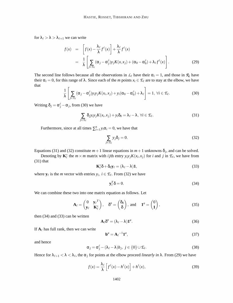
We mimic a simulation found in Marron (2003). We havep = 50 andn = 40, with a 20-20 splitof “+” and “-” class members. Thexi j are all iid realizations from aN(0,1) distribution, except forthe first coordinate, which has mean +2 and -2 in the respective classes.3 The Bayes classifier inthis case uses only the first coordinate ofx, with a threshold at 0. The Bayes risk is 0.012. Figure 10summarizes the experiment. We see that the most regularized models do the besthere, not themaximal margin classifier.

Although the most regularized linear SVM is the best in this example, we notice a disturbingaspect of its endpoint behavior in the top-right plot. Althoughβ is determined by all the points, thethresholdβ0 is determined by the two most extreme points in the two classes (see Section 3.1). Thiscan lead to irregular behavior, and indeed in some realizations from this model this was the case. Forvalues ofλ larger than the initial valueλ1, we saw in Section 3 that the endpoint behavior dependson whether the classes are balanced or not. In either case, asλ increases, the error converges to theestimated null error ratenmin/n.

This same objection is often made at the other extreme of the optimal margin; however, it typi-cally involves more support points (19 points on the margin here), and tendsto be more stable (butstill no good in this case). For solutions in the interior of the regularization path, these objectionsno longer hold. Here the regularization forces more points to overlap the margin (support points),and hence determine its orientation.

Included in the figures are regularized linear discriminant analysis and logistic regression mod-els (using the sameλ` sequence as the SVM). Both show similar behavior to the regularized SVM,having the most regularized solutions perform the best. Logistic regression can be seen to assignweightspi(1− pi) to observations in the fitting of its coefficientsβ andβ0, where

pi =1

1+e−β0−βTxi(44)

is the estimated probability of+1 occurring atxi (Hastie and Tibshirani, 1990, e.g.).

• Since the decision boundary corresponds top(x) = 0.5, these weights can be seen to die downin a quadratic fashion from 1/4, as we move away from the boundary.

• The rate at which the weights die down with distance from the boundary depends on||β||; thesmaller this norm, the slower the rate.

It can be shown, for separated classes, that the limiting solution (λ ↓ 0) for the regularizedlogistic regression model is identical to the SVM solution: the maximal margin separator (Rossetet al., 2003).

Not surprisingly, given the similarities in their loss functions (Figure 2), bothregularized SVMsand logistic regression involve more or less observations in determining their solutions, dependingon the amount of regularization. This “involvement” is achieved in a smoother fashion by logisticregression.

5.3 Microarray Classification

We illustrate our algorithm on a large cancer expression data set (Ramaswamy et al., 2001). Thereare 144 training tumor samples and 54 test tumor samples, spanning 14 common tumor classes that

3. Here we have one important feature; the remaining 49 are noise. With expression arrays, the important featurestypically occur in groups, but the total numberp is much larger.

1408


−4 −2 0 2 4

−3

−2

−1

01

2Optimal Margin

Optimal Direction

SV

M D

irect

ion

+++

+ +

++

+

++++

+

+

+

+

++

++o

oo

o

o

o

o

oo

oo

o

o

oo

o

o

o

o

o

−4 −2 0 2 4

−3

−2

−1

01

2

Extreme Margin

Optimal Direction

SV

M D

irect

ion

+

++

+

++++

+

+

+

+

++

+ ++

+

++

oo

o

o

o

oo

o

oo

o

o

o

o

o

o

o

o

o

o

SSSSSS

SSSSSSS

SSS

SSSSSS

SSSSSSS

SSSSSS

SSSSSSSSSSSSSS

SSSS

S

SSSSSS

100 200 300

2530

3540

Ang

le (

degr

ees)

RRRRRRRRRRRRR

RRRRRRRRRRRRRRR

RRRRRRR

RRRRR

RRRRRRRRR

RRRR

RR

RRRR

LLLLLLLLLLLLLLLLLLLLLLLLLLLLLLLLLLLLLLLLLLLLLLLLLLLLLLLLLLLL

SSSSSSSSSSSSSSSSSSSSSSSSSSSSSS

SSSSSSSSSSSSSSSSSSSSSSS

S

SSSSS

S

100 200 300

0.02

0.03

0.04

0.05

Tes

t Err

or

RRRRRRRRRRRRRRRRRRRRRRRRRRRRRRRRRRRRRRRRRRRRRRRRR

RRRR

RR

RRRR

R

LLLLLLLLLLLLLLLLLLLLLLLLLLLLLLLLLLLLLLLLLLLLLLLLLLLLLLLLLLLL

λ = 1/Cλ = 1/C

Figure 10: p� n simulation. [Top Left] The training data projected onto the space spanned bythe(known) optimal coordinate 1, and the optimal margin coefficient vector found by a non-regularized SVM. We see the large gap in the margin, while the Bayes-optimal classifier(vertical red line) is actuallyexpectedto make a small number of errors. [Top Right] Thesame as the left panel, except we now project onto the most regularized SVM coefficientvector. This solution is closer to the Bayes-optimal solution. [Lower Left] The anglesbetween the Bayes-optimal direction, and the directions found by the SVM (S) along theregularized path. Included in the figure are the corresponding coefficients for regularizedLDA (R)(Hastie et al., 2001, Chapter 4) and regularized logistic regression (L)(Zhuand Hastie, 2004), using the same quadratic penalties. [Lower Right] The test errorscorresponding to the three paths. The horizontal line is the estimated Bayes rule usingonly the first coordinate.

1409


account for 80% of new cancer diagnoses in the U.S.A. There are 16,063genes for each sample.Hencep = 16,063 andn = 144. We denote the number of classes byK = 14. A goal is to build aclassifier for predicting the cancer class of a new sample, given its expression values.

We used a common approach for extending the SVM from two-class to multi-class classifica-tion:

1. Fit K different SVM models, each one classifying a single cancer class (+1) versus the rest(-1).

2. Let [ f λ1 (x), . . . , f λ

K(x)] be the vector of evaluations of the fitted functions (with parameterλ) ata test observationx.

3. ClassifyCλ(x) = argmaxk f λk (x).

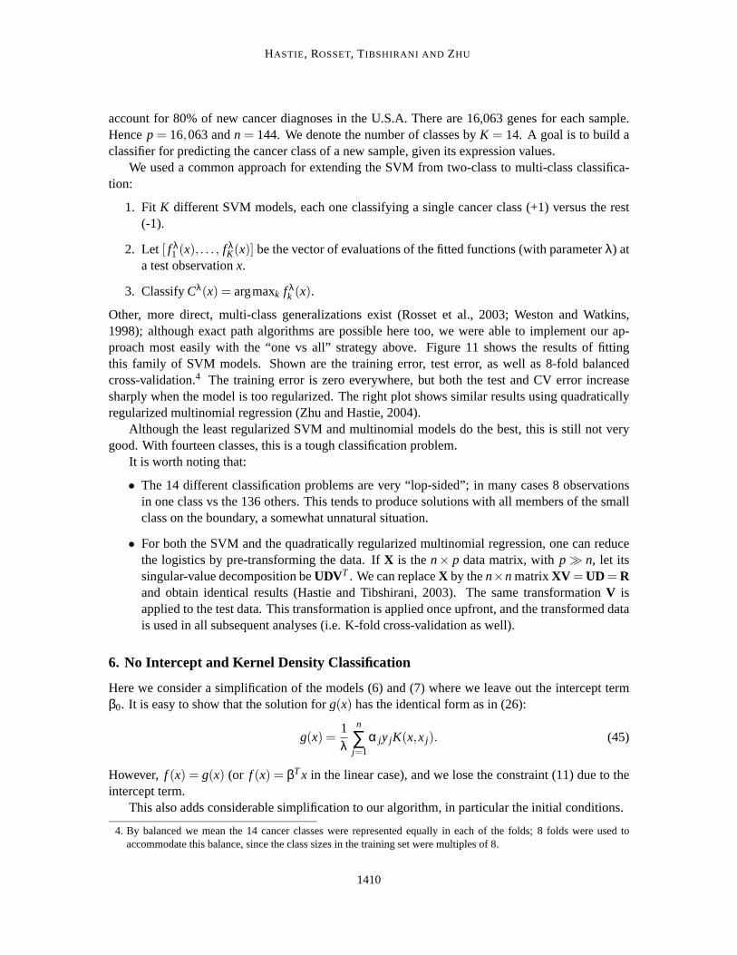
Other, more direct, multi-class generalizations exist (Rosset et al., 2003; Weston and Watkins,1998); although exact path algorithms are possible here too, we were ableto implement our ap-proach most easily with the “one vs all” strategy above. Figure 11 shows theresults of fittingthis family of SVM models. Shown are the training error, test error, as well as 8-fold balancedcross-validation.4 The training error is zero everywhere, but both the test and CV error increasesharply when the model is too regularized. The right plot shows similar results using quadraticallyregularized multinomial regression (Zhu and Hastie, 2004).

Although the least regularized SVM and multinomial models do the best, this is still not verygood. With fourteen classes, this is a tough classification problem.

It is worth noting that:

• The 14 different classification problems are very “lop-sided”; in many cases 8 observationsin one class vs the 136 others. This tends to produce solutions with all membersof the smallclass on the boundary, a somewhat unnatural situation.

• For both the SVM and the quadratically regularized multinomial regression, one can reducethe logistics by pre-transforming the data. IfX is then× p data matrix, withp � n, let itssingular-value decomposition beUDVT . We can replaceX by then×n matrixXV = UD = Rand obtain identical results (Hastie and Tibshirani, 2003). The same transformationV isapplied to the test data. This transformation is applied once upfront, and the transformed datais used in all subsequent analyses (i.e. K-fold cross-validation as well).

6. No Intercept and Kernel Density Classification

Here we consider a simplification of the models (6) and (7) where we leave out the intercept termβ0. It is easy to show that the solution forg(x) has the identical form as in (26):

g(x) =1λ

n

∑j=1

α jy jK(x,x j). (45)

However, f (x) = g(x) (or f (x) = βTx in the linear case), and we lose the constraint (11) due to theintercept term.

This also adds considerable simplification to our algorithm, in particular the initial conditions.

4. By balanced we mean the 14 cancer classes were represented equally in each of the folds; 8 folds were used toaccommodate this balance, since the class sizes in the training set were multiples of 8.

1410


1 10 100 1000 10000

0.0

0.1

0.2

0.3

0.4

0.5

Mis

clas

sific

atio

n R

ates

SVM

TrainTest10−fold CV

1e−02 1e+00 1e+02 1e+040.

00.

10.

20.

30.

40.

5

Mis

clas

sific

atio

n R

ates

Multinomial Regression

λλ

Figure 11: Misclassification rates for cancer classification by gene expression measurements. Theleft panel shows the the training (lower green), cross-validation (middle black, withstandard errors) and test error (upper blue) curves for the entire SVM path. Although theCV and test error curves appear to have quite different levels, the region of interestingbehavior is the same (with a curious dip at aboutλ = 3000). Seeing the entire pathleaves no guesswork as to where the region of interest might be. The right panel showsthe same for the regularized multiple logistic regression model. Here we do not have anexact path algorithm, so a grid of 15 values ofλ is used (on a log scale).

• It is easy to see that initiallyαi = 1∀i, since f (x) is close to zero for largeλ, and hence allpoints are inL . This is true whether or notn− = n+, unlike the situation when an intercept ispresent (Section 3.2).

• With f ∗(x) = ∑nj=1y jK(x,x j), the first element ofE is i∗ = argmaxi | f ∗(xi)|, with λ1 =

| f ∗(xi∗)|. Forλ ∈ [λ1,∞), f (x) = f ∗(x)/λ.

• The linear equations that govern the points inE are similar to (33):

K ∗`δ = (λ`−λ)1, (46)

We now show that in the most regularized case, these no-intercept kernel models are actuallyperforming kernel density classification. Initially, forλ > λ1, we classify to class +1 iff ∗(x)/λ > 0,

1411


else to class -1. But

f ∗(x) = ∑j∈I+

K(x,x j)− ∑j∈I−

K(x,x j)

= n·

(

n+

n·

1n+

∑j∈I+

K(x,x j)−n−n

·1

n−∑j∈I−

K(x,x j)

)

(47)

∝ π+h+(x)−π−h−(x). (48)

In other words, this is the estimated Bayes decision rule, withh+ the kernel density (Parzen window)estimate for the + class,π+ the sample prior, and likewise forh−(x) andπ−. A similar observationis made in Scholkopf and Smola (2001), for the model with intercept. So at this end of the regular-ization scale, the kernel parameterγ plays a crucial role, as it does in kernel density classification.As γ increases, the behavior of the classifier approaches that of the 1-nearest neighbor classifier. Forvery smallγ, or in fact a linear kernel, this amounts to closest centroid classification.

As λ is relaxed, theαi(λ) will change, giving ultimately zero weight to points well within theirown class, and sharing the weights among points near the decision boundary. In the context ofnearest neighbor classification, this has the flavor of “editing”, a way ofthinning out the training setretaining only those prototypes essential for classification (Ripley, 1996).

All these interpretations get blurred when the interceptβ0 is present in the model.For the radial kernel, a constant term is included in span{K(x,xi)}

n1, so it is not strictly necessary

to include one in the model. However, it will get regularized (shrunk towardzero) along with allthe other coefficients, which is usually why these intercept terms are separated out and freed fromregularization. Adding a constantb2 to K(·, ·) will reduce the amount of shrinking on the intercept(since the amount of shrinking of an eigenfunction ofK is inversely proportional to its eigenvalue;see Section 5). For the linear SVM, we can augment thexi vectors with a constant elementb, andthen fit the no-intercept model. The largerb, the closer the solution will be to that of the linear SVMwith intercept.

7. Discussion

Our work on the SVM path algorithm was inspired by earlier work on exact path algorithms inother settings. “Least Angle Regression” (Efron et al., 2002) shows that the coefficient path forthe sequence of “lasso” coefficients (Tibshirani, 1996) is piecewise linear. The lasso solves thefollowing regularized linear regression problem,

minβ0,β

n

∑i=1

(yi −β0−xTi β)2 +λ|β|, (49)

where|β| = ∑pj=1 |β j | is theL1 norm of the coefficient vector. ThisL1 constraint delivers a sparse

solution vectorβλ; the largerλ, the more elements ofβλ are zero, the remainder shrunk toward zero.In fact, any model with anL1 constraint and a quadratic, piecewise quadratic, piecewise linear, ormixed quadratic and linear loss function, will have piecewise linear coefficient paths, which can becalculated exactly and efficiently for all values ofλ (Rosset and Zhu, 2003). These models include,among others,

• A robust version of the lasso, using a “Huberized” loss function.

1412


• TheL1 constrained support vector machine (Zhu et al., 2003).

The SVM model has a quadratic constraint and a piecewise linear (“hinge”) loss function. Thisleads to a piecewise linear path in the dual space, hence the Lagrange coefficientsαi are piecewiselinear.

Other models that would share this property include

• Theε-insensitive SVM regression model

• Quadratically regularizedL1 regression, including flexible models based on kernels or smooth-ing splines.

Of course, quadratic criterion + quadratic constraints also lead to exact path solutions, as in theclassic case of ridge regression, since a closed form solution is obtainedvia the SVD. However,these paths are nonlinear in the regularization parameter.

For general non-quadratic loss functions andL1 constraints, the solution paths are typicallypiecewise non-linear. Logistic regression is a leading example. In this case, approximate path-following algorithms are possible (Rosset, 2005).

The general techniques employed in this paper are known as parametric programming via activesets in the convex optimization literature (Allgower and Georg, 1992). The closest we have seen toour work in the literature employ similar techniques in incremental learning for SVMs (Fine andScheinberg, 2002; Cauwenberghs and Poggio, 2001; DeCoste and Wagstaff, 2000). These authorsdo not, however, construct exact paths as we do, but rather focus on updating and downdating thesolutions as more (or less) data arises. Diehl and Cauwenberghs (2003) allow for updating theparameters as well, but again do not construct entire solution paths. The work of Pontil and Verri(1998) recently came to our notice, who also observed that the lagrange multipliers for the marginvectors change in a piece-wise linear fashion, while the others remain constant.

TheSvmPath has been implemented in theR computing environment (contributed librarysvmpathat CRAN), and is available from the first author’s website.

Acknowledgments

The authors thank Jerome Friedman for helpful discussions, and Mee-Young Park for assistingwith some of the computations. They also thank two referees and the associateeditor for helpfulcomments. Trevor Hastie was partially supported by grant DMS-0204162 from the National ScienceFoundation, and grant RO1-EB0011988-08 from the National Institutesof Health. Tibshirani waspartially supported by grant DMS-9971405 from the National Science Foundation and grant RO1-EB0011988-08 from the National Institutes of Health.

References

Eugene Allgower and Kurt Georg. Continuation and path following.Acta Numerica, pages 1–64,1992.

Francis Bach and Michael Jordan. Kernel independent component analysis. Journal of MachineLearning Research, 3:1–48, 2002.

1413


Gert Cauwenberghs and Tomaso Poggio. Incremental and decrementalsupport vector machinelearning. InAdvances in Neural Information Processing Systems (NIPS 2000), volume 13. MITPress, Cambridge, MA, 2001.

Dennis DeCoste and Kiri Wagstaff. Alpha seeding for support vector machines. InProceedings ofthe Sixth ACM SIGKDD International Conference on Knowledge Discoveryand Data Mining,pages 345–349. ACM Press, 2000.

Christopher Diehl and Gert Cauwenberghs. SVM incremental learning,adaptation and optimiza-tion. In Proceedings of the 2003 International Joint Conference on Neural Networks, pages2685–2690, 2003. Special series on Incremental Learning.

Brad Efron, Trevor Hastie, Iain Johnstone, and Robert Tibshirani. Least angle regression. Technicalreport, Stanford University, 2002.

Brad Efron, Trevor Hastie, Iain Johnstone, and Robert Tibshirani. Least angle regression.Annalsof Statistics, 2004. (to appear, with discussion).

Theodorus Evgeniou, Massimiliano Pontil, and Tomaso Poggio. Regularization networks and sup-port vector machines.Advances in Computational Mathematics, Volume 13, Number 1, pages1-50, 2000.

Shai Fine and Katya Scheinberg. Incas: An incremental active set method for SVM. Technicalreport, IBM Research Labs, Haifa, 2002.

Trevor Hastie and Robert Tibshirani.Generalized Additive Models. Chapman and Hall, 1990.

Trevor Hastie, Robert Tibshirani, and Jerome Friedman.The Elements of Statistical Learning; DataMining, Inference and Prediction. Springer Verlag, New York, 2001.

Trevor Hastie and Rob Tibshirani. Efficient quadratic regularization forexpression arrays. Technicalreport, Stanford University, 2003.

Chih-Wei Hsu, Chih-Chung Chang, and Chih-Jen Lin. A practical guideto support vector classifica-tion. Technical report, Department of Computer Science and Information Engineering, NationalTaiwan University, Taipei, 2003.http://www.csie.ntu.edu.tw/∼cjlin/libsvm/.

Thorsten Joachims. Practical Advances in Kernel Methods — Support Vector Learn-ing, chapter Making large scale SVM learning practical. MIT Press, 1999. Seehttp://svmlight.joachims.org.

Steve Marron. An overview of support vector machines and kernel methods. Talk, 2003. Availablefrom author’s website:http://www.stat.unc.edu/postscript/papers/marron/Talks/.

Massimiliano Pontil and Alessandro Verri. Properties of support vector machines.Neural Compu-tation, 10(4):955–974, 1998.

S. Ramaswamy, P. Tamayo, R. Rifkin, S. Mukherjee, C. Yeang, M. Angelo, C. Ladd, M. Reich,E. Latulippe, J. Mesirov, T. Poggio, W. Gerald, M. Loda, E. Lander, and T. Golub. Multiclasscancer diagnosis using tumor gene expression signature.PNAS, 98:15149–15154, 2001.

1414


B. D. Ripley. Pattern recognition and neural networks. Cambridge University Press, 1996.

Saharon Rosset. Tracking curved regularized optimization solution paths.In Advances in NeuralInformation Processing Systems (NIPS 2004), volume 17. MIT Press, Cambridge, MA, 2005. toappear.

Saharon Rosset and Ji Zhu. Piecewise linear regularized solution paths. Technical report, StanfordUniversity, 2003.http://www-stat.stanford.edu/∼saharon/papers/piecewise.ps.

Saharon Rosset, Ji Zhu, and Trevor Hastie. Margin maximizing loss functions. In Advances inNeural Information Processing Systems (NIPS 2003), volume 16. MIT Press, Cambridge, MA,2004.

Bernard Scholkopf and Alex Smola.Learning with Kernels: Support Vector Machines, Regular-ization, Optimization, and Beyond (Adaptive Computation and Machine Learning). MIT Press,2001.

Robert Tibshirani. Regression shrinkage and selection via the lasso.Journal of the Royal StatisticalSociety B., 58:267–288, 1996.

Vladimir Vapnik. The Nature of Statistical Learning. Springer-Verlag, 1996.

G. Wahba.Spline Models for Observational Data. SIAM, Philadelphia, 1990.

G. Wahba, Y. Lin, and H. Zhang. Gacv for support vector machines. In A.J. Smola, P.L. Bartlett,B. Scholkopf, and D. Schuurmans, editors,Advances in Large Margin Classifiers, pages 297–311, Cambridge, MA, 2000. MIT Press.

J. Weston and C. Watkins. Multi-class support vector machines, 1998. URLciteseer.nj.nec.com/8884.html.

Christopher K. I. Williams and Matthias Seeger. The effect of the input density distribution onkernel-based classifiers. InProceedings of the Seventeenth International Conference on MachineLearning, pages 1159–1166. Morgan Kaufmann Publishers Inc., 2000.

Ji Zhu and Trevor Hastie. Classification of gene microarrays by penalized logistic regression.Bio-statistics, 2004. (to appear).

Ji Zhu, Saharon Rosset, Trevor Hastie, and Robert Tibshirani. L1 norm support vector machines.Technical report, Stanford University, 2003.

1415

Documents

The Entire Regularization Path for the Support …jmlr.csail.mit.edu/papers/volume5/hastie04a/hastie04a.pdf · The Entire Regularization Path for the Support Vector Machine ... (Hastie