Embed Size (px)
Citation preview

i
The Effect of Hydration on the Microstructural Properties of
Individual Phases of Ordinary Portland Cement
Isabella Sharpley
Supervisor: Professor Ian Robinson
1stst April 2015
A Dissertation submitted in part fulfillment for: Degree of MSci Physics:
Dept. Physics and Astronomy
University College London

ii
ABSTRACT
Despite being the most abundant building material in the world, cement still poses
questions regarding its exact composition and hydration properties. An investigation into
the evolution of microstructural properties of OPC during hydration is presented. The
hydration development in the pure phases, Calcium trisilicate (C3S) and Calcium
trialuminate (C3A), is followed using the non-invasive method of x-ray powder
diffraction. The average crystallite size and lattice micro-strain of each sample is
monitored at regular time intervals over to a period of about 2 weeks via the Williamson
Hall method. Careful monitoring of hydration products to deduce the hydration
mechanism is done.
A null result was attained for the average lattice strain in the C3A, and it’s crystallite size
varies throughout the time period but ultimately appears to remain constant throughout.
The C3S crystallite size shows an increase in strain during the initial rapid hydrolysis
phase corresponding to a decrease in crystallite size. The C3A is depleted by
approximately 80% during the 16days of hydration while the C3S shows a 30% decrease
over 11 days.
The results confirm a dissolution along with nucleation and growth mechanism of
hydration

iii
ACKNOWLEDGMENTS
I would like to thank Professor Ian Robinson for his kind supervision throughout the
project, Bo Chen for his continued assistance with sample preparation and Zhuo Feng for
his help in the lab.

iv
Glossary
Ø The following cement nomenclature will be used throughout the report:
C Cao: Free lime
S SiO2: Silica
A Al2O3: Alumina
F Fe2O3: Iron oxide
H H20: water
C3S 3CAO.SiO2 – alite – Tricalcium silicate
C2S 2CaO.SiO2 – Belite – Dicalcium silicate
C3A 3CaO. Al203 – Tricalcium aluminate
C4AF 4CaO.Al2O3. Fe2O3 - ferrite
CH Ca(OH)2 – Portlandite – Calcium hydroxide
C-S-H Calcium Silicate Hydrate
Ø Abbreviations
PC Portland cement
OPC Ordinary Portland Cement
W/C Water to Cement ratio
XRD X-ray diffraction
XRPD X-ray Powder Diffraction
SEM Scanning electron microscopy
TEM Transmission Electron Microscopy
S.A Surface Area W-H Williamson Hall FWHM Full Width Half Maximum

v
Contents Page
Page number Title page……………………………………………………………………….……...i
Abstract……………………………………………………………………………......ii
Acknowledgements……………………………………………………………….…..iii
Glossary…………………………………………………………………………….....iv
Contents page…………………………………………………………………….…....v
1. Introduction ……………………………………………………………………….1
1.1 Purpose and motivation……………………………………………………1
1.2 Objectives and report structure…….………………………………………2
2. Cement structure and hydration chemistry……………………………………...3
2.1 Cement Composition and structure………………………………………..3
2.2 Cement Hydration ………………………………………………………...4
2.2.1 Hydration introduction……………………………………….....4
2.2.2 C3S Hydration…………………………………………………..5
2.2.2.1 C3S Induction period theories……………………..7
2.2.3 C3A Hydration………………………………………………….7
2.2.4 Hydration theories and mechanisms…………………………....8
2.3 Microstructural properties………………………………………………....9
2.3.1 Crystallite size effects……….………………………………….9
2.3.2 Strain……………………………………………………………10
3. Theoretical Background of experimental methods and analysis………………..11
3.1 Intro………………………………………………………………………..11
3.2 Crystal Structure…………………………………………………………...13
3.3 X-Ray Diffraction …………………………………………………………13
3.3.1 X-rays…………………………………………………………13

vi
3.3.2 Bragg and Laue………………………………………………..15
3.3.2.1 The reciprocal space connection…………………16
3.3.3 Powder Diffraction…………………………………………….17
3.3.3.1 Advantages and limitations……………………….18
3.3.3.2 XRP Diffractometer geometry……………………18
3.4 Data Analysis techniques…………………………………………………...19
3.4.1 Average crystallite size and lattice strain determination………19
3.4.1.1 WH analysis………..……………………………..23
3.5 Qualitative and Quantitative phase determination…………………………..24
4. Experiment Methodology……………………………………………………………24
4.1 The Smartlab Rigaku Diffractometer and software………………..………..24
4.2 Sample preparation and schedule of measurements/procedure………..……26
5. Results and discussions……………………………………………………………....29
5.1 C3A…………………………………………………………………………...29
5.1.1 WH Results…………………….……………………………….29
5.1.2 Phase identification……………………………………………..32
5.1.3 Rate of peak growth and decline……………………………….35
5.2 C3S…………………………………………………………………………...36
5.2.1 WH Results…..…………………………………………………36
5.2.2 Phase identification……………………………………………..38
5.2.3Rate of peak growth and decline………………………………...40
5.3 Observations, Conclusions and Improvements…………………………...….41
6. References…………………………………………………………………………….44
7. Appendix…………………..………………………………………………………….48
Appendix 6.1: C3A W-H plots……………………………………………..48
Appendix 6.2 : C3S W-H plots……………………………………………..50
Appendix 6.3: Error calculation equations…………………………………52

1
1. Introduction
From the Egyptian pyramids, across Greek and roman times and throughout the middle
ages [1] cement-based materials have been used for building structures throughout
history. Cement paste (water and cement mix) binds together inert aggregate such as sand
or crushed gravel forming concrete. Concrete based on PC is the most used material in
the world (surpassed only by water) and has an annual production of 7 billion tons [2].
While intrinsically cement is low in energy to produce, due to its mass production,
cement contributes 5-8% of CO2 emissions annually and this is set to increase with
developing countries expanding their infrastructure [3]. Therefore an improvement in the
sustainability of cement is called for and in the future cement composition will likely
need to be adjusted according to the locally available ingredients.
The durability and mechanical properties of cement are a direct consequence of the
microstructure in which a pore network and the proximity of different hydration products
play a key role [4]; therefore it is important to know what’s going on at this level.
An understanding of cement at the microscopic level is essential for the development of
enhanced and environmentally friendly cements, to be attained by the rationalization of
cement properties; for example setting kinetics, strength development and hydration
reactions which are altered by making changes to the composition of cement [5].
Cement is somewhat complex at the microstructural level and there remain unknowns
particularly in relation to the hydration mechanism leading to the setting and hardening of
cement, for which there are several different theories: A topo-chemical (solid state
mechanism) in which the cement clinker liberates Ca2+ ions into solution upon initial
contact with water. The calcium depleted unreacted clinker then reacts with this calcium
rich solution producing hydration products. Versus a through-solution concept where the
anhydrous grains dissolve and hydration products precipitate on the surface of grains[6].
Much research has been focused on the hydration of Portland cement as a whole, and
there are many examples of XRPD studies reported on cement pastes [7].

2
The individual examination of pure phases will allow for a closer look at how the
microstructural properties evolve and are affected during hydration, which will provide
insight into a little piece of a big puzzle. The phases studied in this report are tri-calcium
Aluminate and tri-calcium Silicate (which are the two most important phases controlling
in terms of setting time and strength development during hydration), with the over all aim
being to interpret changes in their physical properties - particularly crystallite size and
lattice strain – over the course of hydration, by careful examination of measured x-ray
diffraction patterns.
Objectives;
• To determine the effect of hydration on the microstructural properties of
pure phases of OPC, by calculation of the average crystallite size and lattice
strain of the water-‐cement phase system as a function of time since the
moment of hydration.
• Careful monitoring of the formation of hydrates as a function of time to gauge
the hydration mechanism.
The report is organized as follows: chapter 2 gives a broad overview of cement
structure, hydration theories and the microstructural properties to be investigated.
Chapter 3 delves into the theoretical background of the X-‐ray diffraction technique
and analysis methods employed
Chapter 4 is a description the experiment performed including and Chapter 5
contains the results and discussions of the findings; what it all means, suggested
improvements and directions of future research.
3
2. Cement Structure and Hydration Chemistry
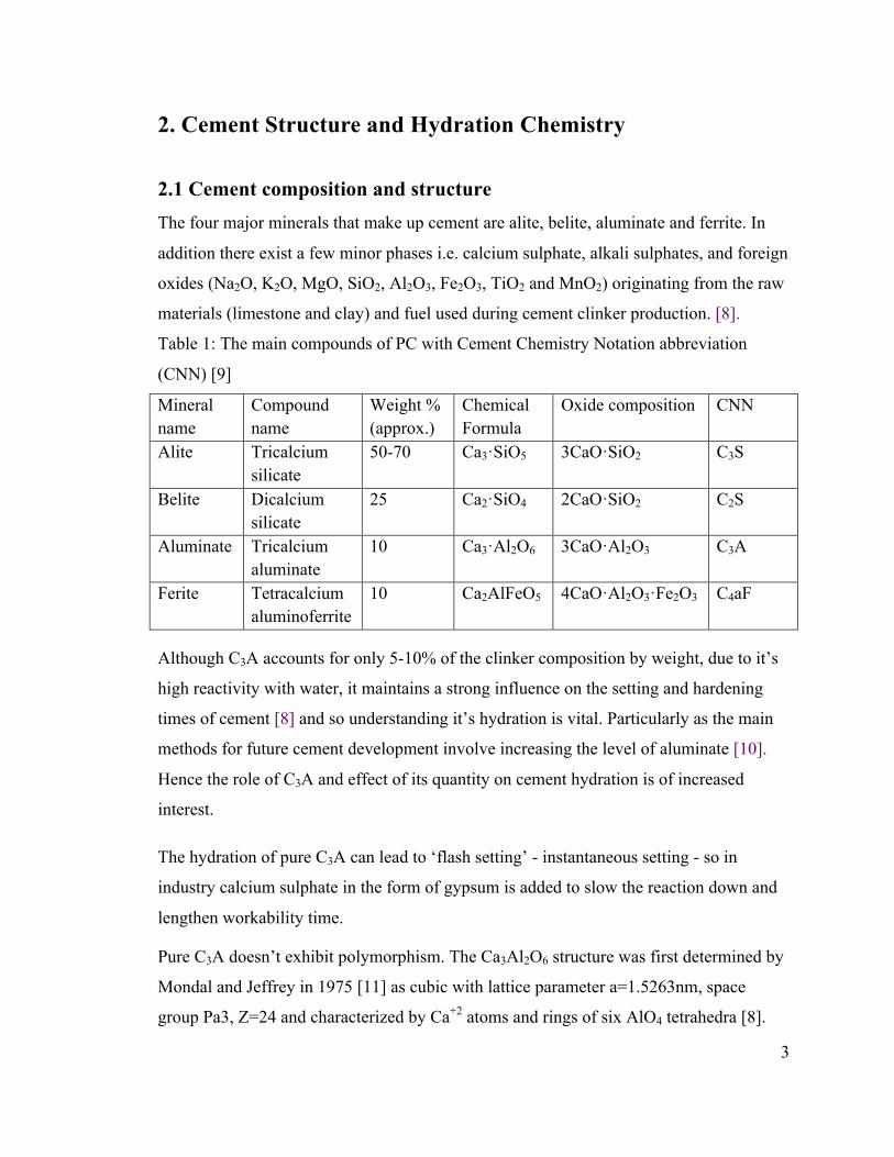
2.1 Cement composition and structure The four major minerals that make up cement are alite, belite, aluminate and ferrite. In
addition there exist a few minor phases i.e. calcium sulphate, alkali sulphates, and foreign
oxides (Na2O, K2O, MgO, SiO2, Al2O3, Fe2O3, TiO2 and MnO2) originating from the raw
materials (limestone and clay) and fuel used during cement clinker production. [8].
Table 1: The main compounds of PC with Cement Chemistry Notation abbreviation
(CNN) [9]
Mineral name
Compound name
Weight % (approx.)
Chemical Formula
Oxide composition CNN
Alite Tricalcium silicate
50-70 Ca3·SiO5 3CaO·SiO2 C3S
Belite Dicalcium silicate
25 Ca2·SiO4 2CaO·SiO2 C2S
Aluminate Tricalcium aluminate
10 Ca3·Al2O6 3CaO·Al2O3 C3A
Ferite Tetracalcium aluminoferrite
10 Ca2AlFeO5 4CaO·Al2O3·Fe2O3 C4aF
Although C3A accounts for only 5-10% of the clinker composition by weight, due to it’s
high reactivity with water, it maintains a strong influence on the setting and hardening
times of cement [8] and so understanding it’s hydration is vital. Particularly as the main
methods for future cement development involve increasing the level of aluminate [10].
Hence the role of C3A and effect of its quantity on cement hydration is of increased
interest.
The hydration of pure C3A can lead to ‘flash setting’ - instantaneous setting - so in
industry calcium sulphate in the form of gypsum is added to slow the reaction down and
lengthen workability time.
Pure C3A doesn’t exhibit polymorphism. The Ca3Al2O6 structure was first determined by
Mondal and Jeffrey in 1975 [11] as cubic with lattice parameter a=1.5263nm, space
group Pa3, Z=24 and characterized by Ca+2 atoms and rings of six AlO4 tetrahedra [8].

4
Alite accounts for 50-70% of the clinker by mass and is known to dominate the early
cement hydration reactions. It reacts relatively quickly in the presence of water and is the
main phase responsible for early strength development in the first 28days [8]. exists as
three different structures; triclinic, monoclinic and rhombohedral. At room temperature
pure C3S has a triclinic structural form. The first determination of it’s structure was made
by Jeffrey (1952) who showed that the polymorphs had similar structures and resolved a
“pseudostructure” common to the three: they are pseudo-rhombohedral with lattice
parameters a=b=~7.0Å, c=~25.0Å, space group R3m and Z=24 [12].
Belite accounts for 15-30% of the PC clinker and is less reactive than alite, contributing
more to strength development beyond 28days. After a year the total contribution to
strength obtained from alite and belite equalize when under similar conditions [8].
Ferrite makes up 5-15% of the clinker [8] and gives cement its distinctive grey colour. It
is moderately reactive; initially reacting quickly with water but the reaction rate slows
over time. The crystal structure of Ferrite, C4AF, is complex. Ferrite is an approximation
of the midpoint of the compositional series Ca2 (AlxFe1-x)2O5 [8].
2.2 Cement hydration
2.2.1 Hydration introduction Hydration is responsible for the ‘setting’, which is the sudden loss of plasticity in the
cement paste due to its conversion to solid material that occurs prior to the development
of compressive strength during the ‘hardening’ (a much slower process) of cement. [13].
During hydration the minerals undergo a complex set of reactions that alter the chemical
and physio-mechanical properties of the system and ultimately form hydrates by
chemically bonding to water molecules. The W/C ratio used in concrete is typically 0.3-
0.6 and greatly influences the resulting strength and workability of the concrete. A higher
ratio gives lower strength due to an increase in the porosity created during the hydration
process, but better workability (and vice versa) [14].

5
When trying to elucidate the hydration mechanism of PC, often the constituent phases are
hydrated individually (as I will be doing) due to the complexity of the mix. In fact Le
Chatelier found that the products produced on the hydration of cement are chemically
identical to those formed by the hydration of the individual components under similar
conditions. [15] This approach was used by Mindess and Young in 1981 [16] .
However the products of hydration may influence each other or themselves interact with
other components in the system, so the hydration of the individual components is more of
an approximation to the real reactions .
2.2.2 C3S hydration C3S hydrates relatively quickly, controlling the setting and hardening of OPC to a great
extent. It’s responsible for early strength development (first 7 days) and typically 70% of
C3S reacts in 28 days and nearly all of it in a year [14].
C3S reacts with water, principally generating a poorly crystalline C-S-H gel and a lot of
calcium hydroxide (also called portlandite, CH) as a secondary hydration product.[14]
2𝐶!𝑆 + 6𝐻 → 𝐶!𝑆!𝐻! + 3𝐶𝐻 (2.1)
The C-S-H composition varies over a wide range, while CH is a crystalline material with
fixed composition.
The hydration of C3S has been widely studied and there exist many theories existing on
potential hydration mechanisms [17]. The hydration of C3S (the main component) and
hence cement generally, can be divided into five stages represented on the following
calorimetry graph from Gartner et al [18].

6
(1) This initial exothermic peak indicates the rapid initial reaction (~15mins) during
which hydrolysis of C3S results in the release of Ca2+ and OH- ions from the surface of
C3S grains. The hydration rate is governed by a topo-chemical mechanism. This
hydrolysis slows down quickly but continues throughout the induction (or dormant)
period.
(2) Indicates the induction period lasting several hours (hydration is almost halted).
Dissolution of ions continues. The reason why hydration is inhibited here is unclear.
(3) Acceleratory period during which C-S-H and CH form via crystallization of ions
when Ca2+ and OH- ion concentrations super saturate. When the products crystallize,
hydrolysis of C3S proceeds again rapidly (nucleation and growth control).
The hydration products provide anchors on which more C-S-H can form, forming a
coating, growing in thickness around the C3S grains. Hence it becomes difficult for water
molecules to reach the anhydrous C3S and the production of hydration products slows
down, as it takes longer for water to diffuse through the coating as observed by [19] who
suggested that C- S-H clusters form by, “heterogeneous nucleation at the C3S surface and
then grow by accumulating C-S-H units.”
Figure2.1 Calorimetry (heat evolution) graph of cement [18]

7
(4) This leads to the period of deceleration (hrs-days) where the hydration is now under
diffusion control.
(5) Diffusion control then continues steadily with a slow deposition of hydration products
(C-S-H and CH) into the pore network, which is the space originally occupied by water.
��������������������2.2.2.1 Induction period theories
While there is general agreement on the framework of hydration, the fundamental
mechanisms governing it ‘aren’t yet fully understood’. For example reasons for the C3S
induction period beginning and ending is subject to several theories including:
1. Initial reaction products forming a ‘protective’ over the C3S particles, which
when destroyed or more permeable indicates an end to the induction period.
[20].
2. A nucleation and growth mechanism of C-‐S-‐H production controls the
reaction rate in the induction and acceleratory periods. The induction period
ending when growth begins.
3. SiO2 poisoning of the CH nuclei causes the induction period. It ends when the
level of super saturation is enough to overcome this and CH products
crystallize.
There is not yet a agreed upon mechanism for what causes the induction period
termination Young et al. [21] observed the end of the induction period to be linked to the
onset of portlandite formation. This supports the nucleation and growth mechanism, with
Ca2+ and OH- concentrations rising until portlandite nucleation happens.
2.2.3 C3A hydration The hydration of pure C3A involves a rapid formation of calcium aluminate hydrates
𝐶!𝐴 + 21𝐻 → 𝐶!𝐴𝐻!" + 𝐶!𝐴𝐻! (2.2)
These hydrates aren’t stable and quickly convert to cubic hydrogarnet 𝐶!𝐴𝐻! [13].

8
𝐶!𝐴𝐻!" + 𝐶!𝐴𝐻! → 2𝐶!𝐴𝐻! + 9𝐻 (2.3)
Where the phase 𝐶!𝐴𝐻!" sometimes exists as 𝐶!𝐴𝐻!" if there is water present in the
interlayer between the hydrate coat and anhydrous grain.
𝐶!𝐴𝐻! has been observed in research papers as an intermediate hydrate by Jupe et al
(1996) [22] and Christensen [23] observed 𝐶!𝐴𝐻!" converting to 𝐶!𝐴𝐻! in C3A-water
systems containing a low amount of gypsum (less than 10 wt%).
While I am looking at pure C3A, in industry Calcium sulphates like gypsum are added to
cement paste to prevent flash setting. Sulphate addition causes ettringite formation, which
is known to form a coating around the anhydrous C3A, grains (similar to the C-S-H
coating observed in C3S hydration), thereby slowing the reaction.
However even with moderate gypsum content, the formation these Calcium Aluminate
Hydrates (also called Afm phases) on C3A grains has been observed at the very start of
the reaction [24], followed by ettringite crystallization. Therefore these hydrates form
regardless of the presence of gypsum as seen in by Pourchet et al. (2009) [25].
2.2.4 Hydration theories and mechanisms
The two opposing theories for the mechanism of cement hydration are the through-‐
solution reaction mechanism and a solid-‐state dissolution theory. According to the
through solution mechanism, the dissolution of anhydrous cement grains when mixed
with water results in a saturated solution from which crystallization of hydrates
transpires. These hydrates cover unreacted grains so that further reaction is controlled
by diffusion of dissolved ions through the barrier. [6]
On the other hand, the solid-‐state theory suggests that the formation of an initial
protective barrier formed from hydrates on the surface of the anhydrous grains
prevents water getting through and the reaction is then controlled by the diffusion of
water through this coating. [26].

9
2.3 Microstructural properties of cement phases
Cement hydration is dependent on the chemical composition, particle size distribution
and W/C ratio.
2.3.1 Crystallite size effects
Polycrystalline materials such as cement mixtures are composed of microscopic
crystallites and the crystallite size can be defined as the size of the “coherently
scattering domains”[27] and can be calculated via XRPD analysis techniques as will be
shown in chapter 3.
The size of the composite particle (and hence contained crystallites) greatly affects its
rate of hydration. Hydration starts at the surface of a particle, so the finer the particles the
greater the surface area (S.A) and hence the rate of hydration is increased [4], resulting in
a more rapid development of compressive strength.
The effect of S.A on the hydration rate supports the fact that dissolution of the anhydrous
grains governs the initial reaction with the nucleation sites of C-S-H on the surface thus
higher surface areas would clearly result in a faster reaction.
Fineness is carefully controlled in industry; an increase in the fineness requires an
equivalent increase in the amount of gypsum due to the increases amount of C3A
available for early hydration [28]. Particle size distribution is therefore critical for
controlling the rate of cement setting and strength development. C3S is the most
abundant phase of OPC, and its particle size distribution directly affects the hydration
kinetics and microstructural properties of cement pastes.
Most previous studies have focused on the overall effects of the S.A and particle size
distribution on hydration kinetics, which is now well understood. However there’s not yet
a good understanding of the influence that particle size has on microstructural
development during hydration with the only relating work by Kondo et al in 1971

10
showing that during hydration the size and the shape of initial C3S grains remain
unchanged [29].
2.3.2 Strain
The micro-‐lattice strain is due to the emerging contact forces between anhydrous
crystallites and hydrates [30]. It is the formation of hydrates in the capillary pore space
of cement-‐water systems that exert forces on one another and on the unreacted grains,
causing strain build up.
Lattice strain is “a measure of the distribution of lattice constants arising from crystal
imperfections” and describes the structural deviation of a crystal due to imperfections
such as lattice dislocations, contact stresses and stacking faults [27].
Further sources of strain could be: thermal strain as a result of the significant liberation
of heat during hydration [31] and shrinkage effects: The total volume of hydration
products is smaller than the combined volume of the reacted cement and water – this is
referred to as “chemical shrinkage” of the cement paste and is the main cause of the
‘self-‐desiccation shrinkage’ which is defined as the bulk shrinkage of cement paste in a
closed isothermal system (i.e. without moisture exchange). This self-‐desiccation is a part
of autogenous deformation in cement and also includes carbonation shrinkage due to
reaction between CH and CO2 in air [32]. Shrinkage during hydration can cause cracks in
building materials. [33]The microstructural changes occurring in the lead up to the
cracking hasn’t been studied à so interrogating the strain of individual phases during
hydration is beneficial to finding the evolution of microstructural change that could
cause shrinkage
W-H plots are used to visualize the contributions of domain size and lattice microstrain
discussed here to the peak broadening in diffraction patterns - see chapter 3.

11
3. Theoretical Background of experimental methods and
analysis
3.1 Introduction
In-situ X-ray powder diffraction will be used to monitor the microstructural properties
(crystallite size and lattice strain) during hydration of C3S and C3A. XRD is used
extensively in the analysis of materials, both crystalline and non-crystalline (amorphous),
to obtain information at the atomic scale. Interpretation of the diffraction patterns,
resulting from the interference of X-rays scattered by atomic planes, provides structural
information i.e. crystallite size, lattice strain and chemical composition of compounds to
name a few [27]. XRD used on PC pastes can prove challenging due to overlapping or
coinciding reflections from the 4 minerals [ 35]. Hence XRD of single phases will help
eliminate this making it easier to spot emerging hydrate products.
XRD is commonly used to investigate cement systems and their hydration. [7].
Advancing XRD technologies and radiation strengths are allowing for more detailed data
to be collected. The theory of XRD is reviewed in this section
Figure 2.2: Schematic of the diffusion of free water through layer of hydrates (the black arrows indicate direction of flow. (modification of diagram from [34]).
Anhydrous grain
Free water
hydrate

12
3.2 Crystal Structure Solids can divided into 3 groups; single crystal, polycrystalline and amorphous
Figure 3.1: Schematic of a single crystal, polycrystal and amorphous atomic positions [43]
In crystals, atoms are arranged periodically in 3 dimensions and possess long-range order
reaching distances greater than the interatomic spacings. For a single crystal the long-
range order is present over the entirety of the specimen. Polycrystalline materials on the
other hand are composed of lots grains (many small single-crystal regions) of different
shapes and sizes, separated by boundaries with the grains on opposing sides of the “grain
boundary” having different orientations with respect to each other [27].
Amorphous materials are “without definite form”, exhibiting only a short-range order that
extends to nearest neighbour atoms. A crystalline material will show sharp peaks
representing x-rays diffracted from the lattice planes, whereas an amorphous material
exhibits a broad peak due to it not possessing long-range order. Hence the amorphous
hydration products e.g C-S-H cannot be directly identified via XRD but is indirectly
indicated through time delays before emergence of crystalline hydration products CH in
C3S hydration or by the presence of a broad “hump” in the background intensity.
A unit cell represents the smallest repeating structural arrangement in a crystal lattice that
can be stacked up to fill 3-D space, with three fundamental vectors mapping it’s 3-D
structure in space relative to the cell origin, given by the lattice vector:[27]

13
𝑅! = 𝑛!𝑎! + 𝑛!𝑎! + 𝑛!𝑎! (3.1)
The side lengths and interaxial angles make up the lattice parameters of a unit cell and
these can be used for identification of a structure. Miller indices identify the crystal
planes in a lattice, which are parallel equidistant planes making intercepts a1/h, a2/k and
a3/l along the 3 crystal axes. [36].
For a cubic unit cell;
𝑑 = !!!!!!!!!
(3.2)
where a is the cell parameter, (h,k,l) are the miller indices and d is the interplanar
spacing. The spacing and orientation of the crystal planes defined by (hkl) are used in
Braggs law.
3.3 X-Ray Diffraction
3.3.1 x-rays
X-rays have energies ranging from 200eV to 1Mev, corresponding to wavelengths
between 10nm and 1pm, which is of the same order of magnitude as the interatomic
spacings of most crystals - usually about 0.2nm (2 Å).[27] X-rays are formed when
electrons produced by heating a cathode (e.g tungsten), are accelerated over a potential
difference towards the target anode, and the energy lost on impact with the anode is
released as x-rays.
The spectrum of x-rays released consist of a spectrum characteristic of the target anode
material - produced when an electron with sufficient energy to eject an inner shell
electron is incident on the target atom, leaving a hole in the atom that is quickly filled by
an outer shell electron causing the release of an x-ray photon with energy equivalent to
the difference between the energy levels. This characteristic spectrum is superimposed
on a continuous background spectrum due to electrons coming to rest in the target after a
series of collisions.

14
Figure 3.3: Shows the characteristic spectrum of copper sourced X-Rays superimposed on the
bremsstrahlung
The inner electron shell is called the K shell, and is followed by the L shell and them M
shell working outwards from the nucleus. When an electron from the L shell fills the hole
in the inner K shell, a Kα x-ray is produced. A Kβ X-ray is released when the ‘hole’ is
filled by an electron from the M shell. Figure 3.4: Schematic of electron shells- here we see the production of a kβ x-ray as the hole in the k
shell is filled by an electron from the m shell. (Source
http://prism.mit.edu/xray)
Kβ x-rays have a higher energy than Kα but Kα
transitions are 10 times more likely due to being closest
to the hole within the k-shell. Now the L-shell consists
of 3 subshells L1, L2 and L3. A transitioning electron
coming from L3 to fill the hole in K emits a Kα1 x-ray
and one from L2 to k emits a Kα2. A Nickel filter with
an absorption edge midway between the Kβ and Kα line
is used in the diffractometer to eliminate (heavily
reduce) the Kβ peak .Kα1 and Kα2 peaks can be seen,
and are easily distinguished at higher 2θ angles where
they are better resolved. [27].

15
3.3.2 Bragg and Laue descriptions Max von Laue discovered that crystalline substances can act as 3D diffraction gratings
for x-rays possessing wavelengths of the same order of magnitude as the interplanar
spacing of crystal structures in 1912 [37].
XRD involves directing an incident wave into a material and recording the outgoing
diffracted wave direction and intensity using a detector. Scattered waves emitted from
atoms of different type and position, interfere constructively or destructively, along
different directions. The crystal structure of a material is related to the directions of
constructively interfering waves, which form the “diffraction pattern” via Braggs Law
[38].
2𝑑𝑠𝑖𝑛𝜃 = 𝑛𝜆 (3.3)
where λ is the X-‐ray wavelength, diffraction angle θ ,lattice spacing ,d of the crystal and
n is the order of diffraction [38]
Figure 3.5: Bragg representation o the diffraction of X-rays from lattice planes (adapted
fromhttp://en.wikipedia.org/wiki/File:BraggPlaneDiffraction.svg)
Braggs law [38] relates the wavelength of the incident x-ray beam to the angle of
diffraction and interplanar plane spacing in the crystal sample.
The diffraction pattern represents a spectrum of real space periodicities in the crystal.
Due to the random orientations of crystals in a powder, all possible diffraction directions
can be obtained by scanning the sample over a 2θ range. Each mineral has a diffraction

16
pattern “fingerprint” and so converting the diffraction peaks to d-‐spacings and
comparing to a standard reference file allows identification of said mineral.[38]
3.3.2.1 The reciprocal space connection
To grasp the physical concept of diffraction, reciprocal space is mentioned. Reciprocal
space maps onto real space through a fourier transformation, and the wave signals
reflected from an atomic plane are the output of a fourier transform of the crystal
lattice. Hence “a point in the reflected space comes from a 3D object in real space”[36].
The reciprocal lattice is a mathematical concept that provides an illustration of the
translational symmetry of crystals. It is derived from the real lattice as a set of vectors
,Gn, perpendicular to the real lattice planes (h,k,l) and with lengths 1/dhkl.
Following on from the real space lattice vector given in (3.1), the reciprocal lattice
vectors are defined as
𝐺! = ℎ𝑎!∗ + 𝑘𝑎!∗ + 𝑙𝑎!∗ (3.4)
where the reciprocal space vectors (𝑎!∗, 𝑎!∗,𝑎!∗) can be derived from the real lattice
vector by
𝑎!∗ = 2𝜋 !!×!!!!.!!×!!
(3.5); 𝑎!∗ = 2𝜋 !!×!!!!.!!×!!
(3.6) ; 𝑎!∗ = 2𝜋 !!×!!!!.!!×!!
(3.7)
The Ewald sphere is a visualization in reciprocal space of the conditions for diffraction to
occur, by superimposing the scattering triangle onto the reciprocal lattice. The observed
Bragg peaks will be from those lattice points that lie on the circumference of the sphere.
Ewald sphere with triangle

17
Figure 3.4: Ewald sphere with scattering triangle
The Laue condition for constructive interference between the incident and scattered
beam, and consequently diffraction to occur is Q=Gn [36].
Where Q is the scattering vector:
𝑄 = 𝑘! − 𝑘! (3.8)
(scattered –incident wavevector; 𝑘 = !!!) and Gn is a reciprocal lattice vector as defined
in equation 3.4 From this we can obtain the Bragg result;
𝑄 = !!"#$%!
= 𝐺! =!!!!!"
(3.9)
−→ 𝜆 = 2𝑑𝑠𝑖𝑛𝜃
3.3.3 Powder Diffraction Measuring a material in powder form results in the random orientation of many tiny crystals with
respect to the x-‐ray beam so there will always be several crystals in the correct orientation for
diffraction according to Braggs law. At any one time there will be many planes each reflecting the
beam along different directions so the powder sample is equivalent to a single crystal being rotated
through all angles. It creates a 1D projection of the 3D reciprocal space which can cause problems
due to overlapping reflections [36] Nonetheless, a unique pattern is produced for a given material
that can be identified by comparison with a database. Bragg Brentano configuration is often used for
powder diffraction.

18
3.3.3.1 Advantages and limitations of XRPD
XRPD inherently averages over many grains and as such is preferred over the TEM
technique for the analysis of grain size and strain in microcrystalline materials.
For XRPD, the material to be analyzed must be ground to an appropriate fineness so as to
minimize primary extinction of the most intense peaks, but not too strongly otherwise it
may lose some crystallinity [39]. Also there must be enough crystals to fulfill the
diffraction condition for each lattice plane. Amorphous phases only serve to increase the
background intensity therefore XRPD doesn’t identify them directly.
3.3.4 The XRP Diffractometer geometry Generally XRPD uses a “Bragg-Brentano” geometry, which allows for illumination of a
reasonable area of the specimen surface. Figure 3.5 Bragg Brentano Beam schematic (source: [40])
Diffractometer’s all have an x-ray source, detector and sample located on the
circumference of the ‘focusing circle’. Another circle known as the diffractometer or
goniometer circle is centered on the sample and has a fixed radius.
Figure 3.6: Bragg Brentano beam optics : DS= Divergent slit, SS= Scattering slit, RS= receiving slit
Detector RS
SS DS
X-Ray Source
sample 2θ
θ

19
In figure 3.6, θ, the Bragg angle, is the angle between the source and sample. And 2θ is
the angle between the projection of the x-ray source and the detector. Hence θ-2θ scans.
In this arrangement the specimen lies flat with the face of the sample forming a tangent to
the focusing circle. This results in some broadening of the diffracted beam and can cause
the Bragg peak position to shift slightly to smaller angles. [41]
After emerging from the x-ray source, the beam passes through soller slits, which are
boxes with many metal sheets parallel to the plane of diffraction. They limit horizontal
divergence of the beam (typically 5°) and the resulting low-theta contribution to peaks.
The length limiting slits simply reduces the horizontal footprint of beam on sample
The divergence slit then chooses the width of the incident beam on the sample. On the
receiving side, after the beam has been diffracted by the sample, it travels through anti-
scatter slits to reduce background noise, improving peak-to-background ratios and
helping the detector to receive x-rays only scattered from the specimen. The beam is then
converged at the receiving slit, towards the detector. The integrated intensity (peak area)
is independent of slit width and is used for phase quantification later on. A scintillation
counter acts as the detector.
3.4 Data Analysis techniques
3.4.1 Average Size and Lattice-strain determination; W-H analysis Following the XRPD measurements of C3S and C3A, the resulting diffraction patterns
will be carefully analyzed using the well-known technique of WH analysis. This section
provides the theoretical details of the technique.
Braggs law assumes that the diffraction takes place under ideal conditions, i.e a perfect
crystal and a completely monochromatic the x-ray beam, resulting in extremely thin
peaks, however in the real world peaks obviously have a measureable width.
The broadening of diffraction peaks arises primarily due to three factors:
1. Instrumental effects: the incident beam divergence and source width.
Unresolved Kα1, Kα2 peaks (luckily the PDXL software deconvolutes these
on automatically and supplies the FWHM of the Kα1 peak)

20
2. Crystallite size: Peaks are broadened due to small crystallite sizes, enabling
peak broadening analysis to be used to determine crystallite sizes in the
range of 100-‐500nm [27]. Supposedly Crystals consist of domains that are
marginally disoriented with respect to each other, hence some domains may
cause diffraction just before the Bragg angle while others are in a position to
diffract just after, thereby broadening the peak.
3. Lattice strain:
This broadening of diffraction peaks causes the peak height to be reduced, while the
FWHM increases thereby maintaining a constant integrated intensity. The Bragg angle
stays constant. The three factors contributing to peak broadening can be separated to find
the average lattice strain and crystallite size values of samples.
Deconvolution of the peak broadening contributions
The first step toward determination of crystallite size and strain is to find the diffraction
breadth that is due to small crystallite size only. The broadening is taken as the width of
the peak at half the maximum intensity of the peak – FWHM.
Let β= observed peak width (FWHM)
βobserved =βinstrumental + βstrain+particle size
βo = βi + βr (3.10)
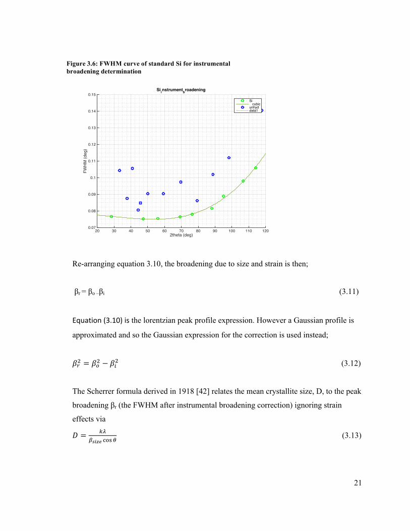
The instrumental contribution to peak width is determined by calculating a FWHM
correction curve by measuring the diffraction pattern of a well annealed powder
(standard Silicon powder was used) sample under the same BB settings.
21
Re-arranging equation 3.10, the broadening due to size and strain is then;
βr = βo –βi (3.11)
Equation (3.10) is the lorentzian peak profile expression. However a Gaussian profile is
approximated and so the Gaussian expression for the correction is used instead;
𝛽!! = 𝛽!! − 𝛽!! (3.12)
The Scherrer formula derived in 1918 [42] relates the mean crystallite size, D, to the peak
broadening βr (the FWHM after instrumental broadening correction) ignoring strain
effects via
𝐷 = !"!!!"# !"#!
(3.13)
2theta (deg)20 30 40 50 60 70 80 90 100 110 120
FWH
M (d
eg)
0.07
0.08
0.09
0.1
0.11
0.12
0.13
0.14
0.15Siinstrumentbroadening
Si cubicunhyddata1
Figure 3.6: FWHM curve of standard Si for instrumental broadening determination

22
It is used for grain sizes in the range 2nm to 300nm and is based on the assumption of
Gaussian peak profiles. K is a dimensionless constant, whose value lies between 0.89 and
1.39 depending on crystallite size and shape. β is the angular width in terms of 2θ
measured in degrees but must be converted to radians in the equation.
The Scherrer equation shows that D and β are related reciprocally – the greater the
broadening, the smaller the crystallite size will be i.e. interference becomes more precise
with increasing number of scattering planes.
Lattice strain also causes peak broadening, with deformations resulting in changes to the
d-spacings, which alters the 2θ positions of diffracted x-rays. For example consider
crystallites compressed equally, resulting in isotropic strain and reducing the d-spacing;
dà d-δd. Then for Braggs law to hold, the peak position needs to increase from 2θ to
2(θ+δθ)
𝜆 = 2𝑑 sin𝜃
𝜆 = 2(𝑑 − 𝛿𝑑) sin(𝜃 + 𝛿𝜃)
Hence in this case the peak position is shifted to a higher Bragg angle.
Uniform strain like this where all crystallites are strained homogeneously, causes a shift
in the peak position only, with no peak broadening effect: simplest strain type and called
“uniform dilatation”. The d-spacings increase slightly under tensile stress, which has the
alternate effect of shifting the Bragg angle to lower values [38].
However in a polycrystalline sample, strains are generally distributed unevenly with
some particles experiencing compression and others tension. This non-uniform strain
causes the grains to be pulled in different directions causing a non-uniform change in the
d-spacing; d-spacing decreases on one side, remaining the same in a defined middle
position and increases on the top planes. Thereby the net effect of this non-uniform strain
is to broaden the resulting diffraction peak. Peaks located at higher Bragg angles exhibit
more broadening than those at lower angles. Non-uniform strain can be caused by point
defects (vacancies, site disorder), plastic deformation and poor crystallinity.

23
Stokes and Wilson (1944) [44] empirically found the broadening from crystallite strain to
be given by:
𝛽!"#$%& = 4𝜀𝑡𝑎𝑛𝜃 (3.14)
Where ε is the strain and θ the Bragg diffraction angle and the strain induced broadening
increases with Bragg angle.
3.4.1.1 WH Analysis
The size and strain broadening contribution vary differently as a function of 2θ and hence
can be separated. Williamson and Hall then proposed a method for deconvolution of the
size and strain broadening to the diffraction peak [45]
Having subtracted the instrumental broadening effect:
𝛽! = 𝛽!"#$%&'( + 𝛽!"#$%& (3.15)
Substituting in the relevant equations
𝛽! =!"
! !!"! + 𝜀 tan𝜃 (3.16)
And multiplying by cosθ,
𝛽! cos𝜃 =!"! + 4𝜀 sin𝜃 (3.17)
This equation has the form of a straight line and so plotting 𝛽! cos𝜃 against sin𝜃 forms a
Williamson-hall plot from which one can estimate both mean crystallite size and lattice-
strain from the gradient and y-intercept of the linear best fit line to the data points.
𝜀 = !"#$%&'(!
(3.18)
𝐷 = !"!!!"#$%&$'#
(3.19)

24
The Williamson hall method is not the most accurate determination of these quantities
but it allows for relative trends to be attained
3.5 Qualitative and Quantitative phase determination
The phases are identified by comparison of the diffraction pattern, d-spacings and relative
peak intensities with the Crystallography Open Database (COD). This can be done using
the autosearch function on the PDXL software. However the autosearch proved erroneous
and it was combined with manual fitting – selecting phases form literature and checking
whether it was a match to the measured data etc.
The growth and decline of phase concentrations is monitored by plotting graphs of the
integrated intensity of a peak representative of a particular phase against time
4. Experiment Methodology
4.1 The Smartlab Rigaku Diffractometer and software X-ray diffraction was performed using the Smartlab Rigaku x-ray diffractometer with
Cu-Kα radiation of wavelength λ=1.5406 Å. The controlling software, “Smartlab
Guidance”, enables the user to select the measurement package – in this case “@General
Bragg Brentano focusing” for powders is used - and guides the user through optical
alignment, sample alignment, slit and scan settings. Fast data collection is enabled by a 9
kW rotating anode source, which produces a high flux of X-ray intensity.
Rigaku Integrated Powder Diffraction Software (PDXL) version 2.2 is used to display the
obtained diffraction patterns. It automatically finds accurate values for the intensity,
FWHM and 2θ position of peaks. PDXL contains many useful functions for data analysis
however only the “Autosearch” and RIR quantification functions were unlocked. The
autosearch function is an algorithim used to compare the degree of coincidence between
the experimentally measured data and data base patterns (COD used). It searches for
major and minor phases until all the peak intensities are matched. However often it

25
identified a phases that the sample clearly was not and so manual search and matching of
the experimental data to database patterns had to be done by finding from literature
expected hydration phases and checking if it matched the measured data.
Figure 4.1: Smartlab Rigaku Diffractometer
To begin with time was spent determining the optimum machine settings to measure the
samples with throughout the investigation and checking that the machine could reliably
reproduce accurate 2θ measurements.
After considering several options, a Bragg Brentano optical configuration (see figure 3.7)
was chosen.
A θ-2θ scan mode is employed where both the x-ray source and detector move in
synchronized motion about the fixed sample stage. The machine was operated at the
maximum load power of 9Kw in order to attain maximum possible intensity to enhance
the counting statistics.
A nickel filter is inserted in the diffracted beam path between the sample and detector, to
eliminate Kβ wavelengths. Kα2 is not removed and we see that peaks split up at higher 2θ
angles. This does not pose a problem because the PDXL software automatically finds the
2θ and FWHM of the kα1 peak.
1. Main panel Panel used to start and stop
SmartLab. 2. Operating panel Panel used to turn the internal
light on/off.
3. Door
This door is opened to change
samples and
optical devices. 4. X-ray warning
lamp
Lights when x-rays are
generated. 5. Door-lock button Lock/Unlock the door. 1 2
3
4
5
Table 4.1: Indicates the name of parts in Fig 1

26
Table 4.2: The BB scan setting used throughout the investigation
4.2 Sample prep:
The samples were prepared by grinding in a pestle until they had the consistency of flour.
If not ground long enough, it was observed that the powder easily fell out of the trench.
For the C3A sample that came in a solid block form, clean pliers were used to break off
fragments that were then ground up in the pestle.
Figure 4.2: Pestle used to grind sample
The powdered sample is then carefully deposited into a rectangular glass sample holder
of trench depth 0.2mm using a spatula and smoothed level in the trench using a
microscope slide. Note: Protective gloves and glasses were worn, and all apparatus
thoroughly cleaned and dried using ethanol prier to preparation.
The mass of sample within the trench is then measured using scientific scales so that the
sample phase can be hydrated with 0.5 W/C-ratio using a biological 20-200micro-litre
Finn pipette.
Pritt-stick glue is applied around the sample trench and commercial cling film pulled taut
to cover the sample immediately following hydration (likewise when the unhydrated scan
is done) – this is done to help minimize irreversible hydration/carbonation of the sample
IIncident Parallel Slit
slit Incident
slit
Length
limiting
slit
Receiving
slit 1
Receiving
slit 2
Receiving
optical
device
Receiving
parallel slit
attenuator
S Soller slit 5 deg 2/3 deg 10mm 2/3 deg 0.3mm PSA_Open Soller slit 5
deg
open

27
due to exposure to the atmosphere. The use of clingfilm served to only very slightly
reduce the overall intensity, peak positions were unaffected.
To follow the microstructural changes and phase evolution, measurements were taken at
regular time intervals: The following schedule of measurements was stuck to as far as
possible. (Note the machine was turned off for 3 weeks in January and had many other
users which halted measurements)
Time scale of measurements to undertake for the C3S and C3A samples:
unhydrated, 1h, 2h, 3h, 6h, 12h, 24h/1d, 3d, 5d, 7d, 10d, 14d, 18d,
(h=hour, d=day).
Scan lengths were adjusted according to the length of time passed:
Unhydrated sample: 30min + 1hr scan
The measurements once the sample has been hydrated were:
Up to 24h: 30min scan; to allow quick collection as this is where reaction is fastest.
1d-7d: 30min scan + 1hour scan;
beyond 7d: 30min scan + 2hour scan.
However in the end as rietveld refinement was not performed these long measurements
were unnecessary but did however help when identifying phases with accuracy.
In between measurements the samples were kept in air tight plastic bags within airtight
plastic boxes to provide protection from the atmosphere.
Samples were scanned over a range of 5° to 125°, with a 0.01° step widths and a scan
speed of 4° per minute (for 30min scan), 2° per min for the 1hr scan and 1° per minute
for the 2 hour scan. The temperature is assumed to be kept constant within the chamber
~Room Temperature (25°).

28
These measurement settings provided good counting statistics however due to the length
of each scan (30 mins to 2 hours at later stages), the scan does not exactly represent the
phase hydration time accurately.
Fig 4.3; Shows the sample held in the Height reference sample plate in the Smartlab
diffractometer.
The sample is inserted into the height reference sample holder as shown in fig 4.3 and is
fixed in place by clips. No sample height alignment is required as it is at the axis
reference height.
Optical alignment is carried out before each new measurement. It finds the offset in 2θ
and ω and corrects (zero’s) them.
An attempt at hydrating the sample via a humid environment as opposed to direct
hydration was done by placing a water bath in close vicinity to the sample in an enclosed
environment using cling film. It results in much slower hydration rate and so was not
employed further.
Throughout the investigation measurements of the Si reference sample were taken
regularly to identify trends in any peak shift occurring and check that the peaks are
correctly agreeing with database values and are reproducible.
See appendix 3 for a discussion and calculation of the uncertainties involved in taking
measurements using the Smartlab diffractometer

29
5. Results and discussions
5.1 C3A
The peak positions and FWHM’s obtained by PDXL are used to calculate the average
crystallite size and lattice-strain, while the integrated peak intensities are used to see the
rate of reactions and growth/decline of a phase.
5.1.1 WH results
The WH plots were plotted in excel by selecting a range of peaks across the
diffractogram range 5-125° that were present during the whole 16day period. These peaks
were manually tracked and then the W-H plots built. The y-intercept and gradient of the
best fit line was found accurately using the LINEST function. The majority of plots
resulted in negative linear fits indicating non-physical negative strains. Therefore it is
considered to be a null result without strain[46]. Calculating the associated errors, we see
that a horizontal fit (to indicate zero strain) is within the experimental uncertainty of the
data points The full set of plots can be seen in appendix 1 along with explanation of
errors and error propagation in appendix 2.
Graph 5.3 W-H plot at 1hr hydration of C3A with extrapolated horizontal fit shown to be
within error bars.
y = -‐0.0005x + 0.001 R² = 0.21249
0 0.0002 0.0004 0.0006 0.0008 0.001 0.0012 0.0014
0 0.5 1 1.5 2 2.5
Bcosθ
sinθ
1hr
1hr
Zero Strain
Linear (1hr)

30
However the average crystallite size obtained from the W-H plots correlates with that
obtained when strain is not taken into account by using the Scherrer formula (see graph
5.1). The Scherrer formula is used to calculate the average crystallite size of the same
range of peaks as used for the W-H analysis.
Table 5.1: values obtained for the average crystallite size and lattice strain of the C3A at
designated times up to 16 days via the W-H graphical method and when eliminating
strain via the Scherrer formula
Time
(hrs)
W-‐H Average crystallite
size (x10-‐7m)
W-‐H Average
lattice strain x10-‐4
Average
crystallite size
from Scherrer
only (x10-‐7m)
Crystallite size
from horizontal
fit (x10-‐7m)
unhyd 0.1 1.51 -‐0.911 1.98 1.931
1hr 1 1.38 -‐1.16 1.87 1.931
2hr 2 1.06 -‐2.2 1.78 1.6091
3hr 3 1.91 0.341 2.07 1.788
6hr 6 1.28 -‐0.616 1.55 1.448
12hr 12 2.53 1.2 2.05 1.45
20.5hr 20.5 2.32 0.342 3.27 1.48
3days 72 4.49 2.54 4.04 1.33
5days 120 2.16 1.54 1.96 1.29
7days 168 0.781 -‐3.41 1.47 1.43
10days 240 1.19 -‐0.971 1.99 1.46
16 day 384 0.993 -‐2.96 2.20 1.61

31
Graph 5.1: comparing the evolution of crystallite size when strain is considered (W-H)
and when neglected i.e. zero strain using Scherrer. Use of a log scale for time.
Interestingly the average crystallite size obtained for both methods follows the same
projection with time – both show the crystallite to decrease in size initially before
reaching a maximum size at 3days and then decreasing to a minimum value at 7days and
rising slightly to what appears to be a steady size. The final size is smaller than the
original size for W-H, and larger by a little for the Scherrer.
Graph 5.2: Shows the evolution of crystallite size calculated via the scherrer formula
using only individual peaks that represent C3A (log scale for time)
0
1
2
3
4
5
0.1 1 10 100 1000 Average crystallite size
(x10
-‐7m)
Time (hrs) since hydration
Evolution of Avg. C3A Crystallite size from W-‐H and Scherrer
W-‐H Avg. Crystallite size
Avg. Scherrer size
0
5
10
15
0.1 1 10 100
Crystallite size (x10
-‐7m)
Time since hydration (hrs)
Evolution of crystallite size of single C3A Peaks via scherrer
~33.2
~59.3
~69.6

32
While the peak at ~59.3° stays steady, the others shows a sharp rise in crystallite size at
3days and 5days for the ~69.6° and ~33.2° peaks respectively.
5.1.2 Phase identification
The diffraction patterns obtained from the diffractometer are displayed on the PDXL
software. Savitzky-Golay smoothing and background intensity subtraction is done before
matching to the database. The unhydrated diffraction pattern was identified as calcium
cyclo-hexaluminate ; Ca9(Al6O18),which is C3A (same crystal structure as Ca3Al2O6)
The first diffraction pattern obtained after 1hrs hydration shows a noticeable decrease in
peak intensity of the C3A indicated it’s high reactivity with water
Diffractogram 5.1: unhydrated and 1 hr diffraction patterns
On removal of the background intensity, there is a clear hump revealed in the range 15-
20° and one around 7°. These may correspond to an amorphous phase. They are also
present in the unhydrated scan so exposure of sample to atmosphere on preparation
(grinding did take 15 minutes) and inadequate sample storage has perhaps lead to some
water attack.
Meas. data:UnhydratedMeas. data:1hr
2-theta (deg)
Inte
nsity
(cou
nts)
20 30 40 50 60
1000
2000
3000 4000 5000 6000

33
Diffractogram 5.5: Background intensity humps indicate possible amorphous phase
present
Hydrogarnet is matched to the peak at 44.39° and a trace amount of carbonated calcium
hemicarboaluminate is picked up at 52.59° (indicates carbonation of sample) at 1hr.
This hydrogarnet peak only increases noticeably in intensity from 2hrs, at 2hrs other
hydrogarnet peaks begin to emerge at 17.3°, 26.4°,28.4°,39.2°, 53.5° and 54.6°.
Diffractogram 5.6: continued increase in intensity of hydrogarnet and decline of original
C3A
Meas. data:UnhydratedMeas. data:1hr
2-theta (deg)
Inte
nsity
(cou
nts)
10 20 30 40 0
1000
2000 3000 4000 5000 6000
Meas. data:UnhydratedMeas. data:2hrMeas. data:3hr
2-theta (deg)
Inte
nsity
(cou
nts)
38 40 42 44 46 48 50 52 54 56 58 0
500
1000
1500
Amorphous phase?
Hydrogarnet
Hydrogarnet

34
Hydrogarnet peak growth is significant at 3hrs (in fact peaks have doubled in intensity
within the hour). All hydrogarnet peaks emerge mostly from 2hrs except the 44.39° peak
which appears at 1hr , appearing to grow on top of a peak around present in the
unhydrated sample. )
Diffractogram 5.7: Hydrogarnet peaks (in pink here) reach a maximum intensity at 12hrs,
at which point the C3A (Blue) is also maximally depleted
Diffractogram 5.8: At 16days most of the original C3A peaks are more or less completely
depleted except for the very strong 33.2° peak which remains present throughout;
Meas. data:UnhydratedMeas. data:1hrMeas. data:2hrMeas. data:12hr
2-theta (deg)
Inte
nsity
(cou
nts)
34 36 38 40 42 44 46 48 50 52 54 0
500
1000
1500
Meas. data:UnhydratedMeas. data:2hrMeas. data:16days
2-theta (deg)
Inte
nsity
(cou
nts)
32 34 36 38 40 42 44 46 48 50 52 54 56 0.0e+000 1.0e+003
2.0e+003
3.0e+003
4.0e+003
5.0e+003

35
Diffractogram 5.9: the suggested ‘amorphous’ hump remains
5.1.3 Rate of peak growth and decline
Plotting the integrated intensity against time, gives an indication of the rate of reaction as
well as phase developments in the hydrating system and the quantities of constituent
phases remaining and emerging.
Graph 5.3: shows the decrease in concentration of the major (highest intensity) C3A peak
located at 33.2°. This has a rapid decline in the first few hours and begins to reach a
steady level at 3hours. Immediate growth of the hydrogarnet hydrate product is seen from
1hr with the peak at 44.3°. The hydrogarnet reactions show rapid growth around 6hours
and reach a maximum at ~12hours where they collectively level off having reached a
steady state. The rapid growth phase of the hydrogarnet (between 3-12hours), occurs ~
Meas. data:UnhydratedMeas. data:1hrMeas. data:2hrMeas. data:16days
2-theta (deg)
Inte
nsity
(cou
nts)
6 7 8 9 10 11 12 13 14 0
200
400
600
800
1000
-‐100 0
100 200 300 400 500 600 700
0.1 1 10 100 1000
Integrated intensity (counts deg)
Time since hydration (hrs)
Decline of C3A and Hydrogarnet growth c3a (~33.2)
Hydrogarnet (~39.2)
hydrogarnet (~44.3)
Hydrogarnet (~17.2)

36
3hours after the rapid C3A decline. This indicates that following the quick dissolution of
the C3A in the first 3hours since hydration, there is a dormant period for a few hours
before hydrogarnet crystallizes out in mass. i.e supports the theory of nucleation and
growth.
The steady state intensity begins to slowly decline (decelaratory phase), probably due to
the depletion of C3A or less S.A of the C3A grains being available for reaction due to
more of C3A surface touching the crystalline hydrates – i.e the reaction rate is now
diffusion controlled
5.2 C3S results
5.2.1 WH
C3S on the other hand gives realistic physical values for the average crystallite size and
lattice strains from the W-H plots.
Table 5.2: displaying the average C3S crystallite size and lattice strain values obtained
via the WH method and the size with the Scherrer formula
Measurement Time (hrs) W-‐H Average crystallite size (x10-‐7m)
W-‐H Average lattice strain (x10-‐4m)
Scherrer Average crystallite size (x10-‐7m)
unhydrated 0 1.46 5.71 1.04 1hr 1 1.55 7.71 0.788 2hr 2 1.92 8.53 0.759 3hr 3 1.01 25.2 0.723 6hr 6 2.79 10.7 0.777 12hr 12 0.878 2.35 0.807 1day 24 1.45 5.82 0.991 2days 48 1.29 6.53 0.793 3days 72 1.07 3.86 0.843 7days 168 1.00 5.82 0.679 9days 216 1.30 6.82 0.829 11days 264 2.95 8.74 1.45
The average crystallite size of the C3S decreases initially up to 3hrs and this correlates
with an increase in the average lattice strain which reaches a maximum at 3hrs; this could
correspond to the rapid dissolution of the C3S resulting in increased ion concentrations

37
and the formation of crystalline hydrates emerging into the pore network of the system,
producing contact forces on the unhydrated C3S and therefore increasing strain. At 6hrs
C3S shows a sudden increase in size along with a decrease in strain.
However after 6hrs the strain appears to be almost proportional to the crystallite size –
increasing and decreasing correspondingly. This result is somewhat different to that of
Kondo et al in 1971 [29] who showed the size of C3S to be unchanged – however here we
see a marked increase in crystallite size at 6hrs and 11 days. It is difficult to develop any
trends in the data without further complementary experimental techniques to confirm the
size increase at these two times.
In comparison using the Scherrer formula to estimate crystallite size results in
consistently smaller size values – this is expected because the Scherrer formula doesn’t
take into account the effect of lattice strain on peak broadening, and hence overestimates
the peak broadening due to crystallite size causing the crystallite size to be
underestimated .It does however follow broadly similar trends to the WH size: decreasing
initially with the low value at 3hrs before increasing slightly to around 0.991 at 1 day and
then more or less staying a steady size until a marked increase at 11days.
Graph 5.4: shows the progression of average C3S crystallite size and lattice strain as
0
5
10
15
20
25
30
0
0.5
1
1.5
2
2.5
3
3.5
-‐1 4 9 14 19 24
Average crystallite size
(x10
-‐7m )
Time (hrs) since hydration
Evolution of average W-‐H C3S Crystallite size and strain
0
5
10
15
20
25
30
0
0.5
1
1.5
2
2.5
3
3.5
24 74 124 174 224 274
Average Lattice Strain x10
-‐4
Size
Strain

38
5.2.2 Phase identification
The PDXL autosearch function correctly identifies the unhydrated C3S diffraction pattern
correctly as Hatrurite (Ca9 O15 Si3). Very slow reaction rate compared with C3A . There is
an unidentified peak emerging from what appears to be an amorphous hump in the
background intensity at around 7°. C3S peaks are only slightly reduced at 1hr hydration
as shown in diffractogram 5.10
Diffractogram 5.10: The peak at 7° grows while other peaks decrease in intensity.
Diffractogram 5.11: The first indication of hydrate formation is at 12hrs with the
appearance of a peak at 17.9° representing portlandite.
Meas. data:UnhydratedMeas. data:1hr
2-theta (deg)
Inte
nsity
(cou
nts)
10 20 30 40 0
500
1000
Meas. data:UnhydratedMeas. data:1hrMeas. data:3hrMeas. data:6.5hrsMeas. data:12hr
2-theta (deg)
Inte
nsity
(cou
nts)
6 8 10 12 14 16 18
0
200
400
600
800
CH
Unknown – maybe amorphous hydrate

39
Diffractogram 5.12: The 17.9° CH peak reaches its maximum intensity at 24hrs and at
24hrs there is an additional portlandite peak that emerges at 2θ=33.9°
Diffractogram 5.13:CH peak at 33.9° emerges at 24hours and grows as indicated in graph
C3S intensity decreases immediately on hydration, albeit slowly and there is a delay
before CH forms: either it’s taking a long time for the C3S to hydrolyze and calcium and
hydroxide ions to supersaturate in order for CH to finally crystallize out, or this could
indicate an intermediate phase causing the delay, perhaps an amorphous C-S-H coating
the C3S, causing reduced hydrolysis and a diffusion limited reaction. Would require more
measurements at closer time intervals and use of TEM/SEM to see the phases
microscopically to confirm this.
Meas. data:UnhydratedMeas. data:1hrMeas. data:3hrMeas. data:12hrMeas. data:1day
2-theta (deg)
Inte
nsity
(cou
nts)
10 15 20 25 30
0
200
400
600
800
Meas. data:UnhydratedMeas. data:3hrMeas. data:12hrMeas. data:1dayMeas. data:3daysMeas. data:1 weekMeas. data:11days
2-theta (deg)
Inte
nsity
(cou
nts)
30 35 40 45
0
200
400
600
800
CH
CH

40
5.2.3: Rate of peak growth and decline
Graph 5.5: Integrated intensity of C3S and CH phases plotted as a function of time
While the decreasing C3S peaks do end up losing about 1/3 of their original intensity over
the period of 11days hydrating (we know that 70% of C3S reacts in the first 28 days[8]),
the decline is rather variable for all C3S peaks identified. The intensity decreases during
the first hour of hydration but then increases again reaching a high point between 6.5 and
24 hours, followed by further demolition, then a slight plateau before further rapid
decline. This may be a result of placing the sample back in the diffractometer for
measurement, at a slightly different position to the previous measurement, where less
sample has reacted, therefore making the C3S appear to increase in intensity. The major
portlandite peak at 17.9° emerges at 12hrs hydration i.e. directly following the rapid
decline of C3S peak 34.3° and 51.6°. The only other CH peak is observed at 24hours and
this roughly corresponds to a second decline phase of the 51.6 peak.
-‐50
0
50
100
150
200
0.1 1 10 100 1000
Integrated Intensity (Counts deg)
Time since hydration (hrs)
Decline of C3S and growth of Portlandite
C3S (~32.2)
CH (~17.9)
C3S (~51.6)
CH(~33.9)
C3S (~34.3)

41
5.3 Observations, conclusions and improvements
From observations of when hydration products appear in the diffraction patterns: We see
a rapid hydrolysis of both C3A and C3S phases, which slows down at about 2hours in
C3A and 6hrs in C3S. There is an clear induction period in the C3S before products of
portlandite crystallize out at 12hrs. No direct observation of amorphous C-S-H phases
detected however can speculate that the presence of some undetected hydrate phase
causing the prolonged induction period. The C3A on the other hand reacts rapidly and
hydrogarnet forms immediately, increasing its rate of formation at ~3hrs which is when
C3A begins to reach a steady state. There is no intermediate metastable calcium aluminate
hydrate formation detected.
Unfortunately there is no defined trend relating to the average crystallite size to the lattice
strain in C3A due to the null result obtained from the WH plot as a result of the negative
non-physical strain. However both the WH and Scherrer determination of the crystallite
size for C3A agree that the crystallite size decreases over time showing a total decrease
from 1.50x10⁻⁷ m to 0.993x10⁻⁷m according to WH (with which zero strain was found),
from 1.931x10⁻⁷m to 1.61x10⁻⁷m from the graphical estimation using a horizontal fit
through the WH plot, and appears to remain approximately the same size according to the
Scherrer formula.
It is also difficult to obtain any solid trend from the C3S data where the strain increases to
a maximum at ~6hours, yet the CH crystallite hydrates don’t appear until 12hrs, so this
increase in strain is perhaps and indication of the presence of an this unidentifiable C-S-H
phase with which C3S is experiencing contact force, and is speculated to be causing the
induction period before growth of CH at 12hours.
Therefore a nucleation and growth process appears to be the controlling step in general
hydration, while diffusion through a hydrate layer controls the later steady state stages of
the hydrates formed.
The average C3S crystallite size appear to remain around the initial unhydrated value
throughout except for an increase of 3 fold at 6hrs according to WH only and an increase

42
on the final measurement at 11days according to both WH and Scherrer calculations –
these appear random. Would have to take further measurements and plot WH graphs
relating to specific (hkl) planes to interrogate this issue further.
Observations of the growth rates of hydrate phases, portlandite and hydrogarnet from
C3A and C3S respectively confirm the findings of previous research on mechanisms
responsible for the hydration process; such as the Minard et al’s findings [48] that the
hydration rate is first under chemical control according to the dissolution of C3A which
first depends on the surface area of the grains and then the space available, given the
amount of hydrates already precipitated into the porous capillary networkspace ài.e it’s
all about the amount of C3A surface exposed to water. The rate will decrease when
hydrates touch C3A grains thereby minimizing the surface area exposed. And for C3S,
Young et al’s work (1977) [21] is confirmed: The nucleation and growth mechanism
whereby calcium and hydroxide ion concentrations rise to a high enough level for
crystallization of CH to occur is supported by the C3S findings which indicate that the
induction period ends when CH crystallization commences (at 12hours according to my
results, which is much longer than the usual ~3hours).
In conclusion, the effect of hydration on the OPC phases C3S and C3A is taken to be a
continuing hydrolysis of the anhydrous grains that causes the ions liberated to saturate the
solution and hydration products, Hydrogarnet Portlandite to crystallize out into the pore
space previously occupied by water. This has the effect of increasing the micro strain of
the sample as observed in the first 6hrs of C3S hydration.
The rapid formation of Hydrogarnet and CH between 6hrs and 24hrs indicates many
microstructural change occurring and is represents of the acceleration period. The
induction period lasts ~12 hrs in the C3S sample, which is far slower than normal – this
could be due to inadequate combining of the sample with water as water was pipetted
onto samples rather than mixed thoroughly.

43
Improvements
Cement systems are complex and there are a vast number of analysis techniques that can
be performed on such systems. Preparation could have been more precisely done – i.e.
storing samples in an atmosphere-less environment, using a machine to perform
powdering of particles and measure the size externally to check the results are on track.
A disadvantage of using XRD to monitor the hydration is the length of time that it takes
to obtain a diffraction pattern with the appropriate count statistics for identification. A
synchrotron radiation source would be required to obtain data fast enough for an
investigation of the very early moments of hydration where an acquisition speed of
minutes would be necessary! Other methods to enhance the time resolution of
measurements and make them more “in-situ” could be using a more efficient detector or
use of acetone to freeze the hydration in its tracks.
Also as the diffractometer had many other users taking various measurements, this may
have altered the machine alignment slightly – adding a level of uncertainty to the
measurements. Therefore it would be good to repeat the experiment with the
improvements mentioned above and also make use of other experimental techniques,
such as SEM, TEM and calorimetry in conjunction with the XRPD to estimate the
crystallite size and strain and thereby provide confirmation of the XRPD findings. Also
use of alterative analysis techniques such as the Warren-Averbach method for separating
size and strain effects [48].

44
6. REFERENCES
[1] F. Lea, “Lea’s Chemistry of Cement and Concrete”, Arnold publishers, edited by Peter C. Hewlett , 4th edition, 1998 , Ch.1 [2] “What is the development impact of concrete?” Cement trust, http://cementtrust.wordpress.com/a-concrete-plan [3] Scrivener, K. L. “The Concrete Conundrum”. Chemistry World, March 2008, p. 62−66 [4] F. Lea, “Lea’s Chemistry of Cement and Concrete”, Arnold publishers, edited by Peter C. Hewlett , 4th edition, 1998, Ch.8 [5] Flatt. R. J, Roussel. N Cheeseman.C.R ,“Concrete: An Eco Material that Needs to be Improved.”, Journal of the European Ceramic Society, 2012. 32; p.2787−2798. [6] Lamour, V.H.R.; Monteiro, P.J.M.; Scrivener, K.L.; Fryda, H. “Microscopic studies of the early hydration of calcium aluminate cements”, International Conference on Calcium Aluminate cement (CAC), Edinburgh, UK, 2001; p.169-180. [7] M. Merlinia, G.Artioli, “The early hydration and the set of Portland cements: In situ X-ray powder diffraction studies” ,Powder Diffr., September 2007, Vol. 22, No. 3.
[8] H.F.W. Taylor, “Cement Chemistry”, Thomas Telford, London, 2nd Ed., 1997, ch. 1. [9] A.M.Neville, “Properties of concrete”, Pearson Education Limited, 5th Ed., 2011, p.8 , table 1.1“Main compounds of Portland cement” . [10] K.l. Scrivener, “Options for the future of cement”, The Indian Concrete Journal, July 2014, Vol. 88, Issue 7, p. 11-21 [11] Mondal, P. and Jeffery, J.W. “The crystal structure of tricalcium aluminate, Ca3Al2O6”, Acta Cryst. 1975. B31, p.689-697. [12] Jeffry, J.W.,”The crystal structure of tricalcium Silicate” Acta cryst. 1952, Vol. 5, p.26-35. [13] F. Lea, “Lea’s Chemistry of Cement and Concrete”, Arnold publishers, edited by Peter C. Hewlett , 4th edition, 1998, Ch.6. [14] H.F.W. Taylor, “Cement Chemistry”, Thomas Telford, London, 2nd Ed., 1997, Ch.5. [15]A.M. Neville, “Properties of Concrete”, Pearson Education Limited, 5th Ed, 2011, p. 13. [16] Mindess, S.; Young, J.F. (1981). Concrete. Englewood, NJ, USA: Prentice-Hall. ISBN 0-13-167106-5. [17] Juilland, P., et al., “Dissolution theory applied to the induction period in alite hydration.” Cement and Concrete Research, 2010. 40(6): p. 831-844. [18] Gartner, E.M., et al., eds. “Structure and Performance of cements”, 2nd edition, Spon Press ed. 2002. Ch.3.

45
[19] Garrault, S. and A. Nonat, “Hydrated Layer Formation on Tricalcium and Dicalcium Silicate Surfaces: Experimental Study and Numerical Simulations.” Langmuir, 2001. 17(26): p. 8131- 8138. [20] Jennings, H.M. “Aqueous Solubility Relationships for Two Types of Calcium Silicate Hydrate”, J. Am. Ceram. Soc. (1986) 69, p. 614-618] [21] Young et al. “ Composition of solutions in contact with hydrating β-Dicalcium Silicate”, J. Am. Ceram. Soc.,(1977), 60, p. 321-323. [22] Jupe, A.C., et al., “Fast in situ x-ray-diffraction studies of chemical reactions: A synchrotron view of the hydration of tricalcium aluminate.”, Physical Review B, 1996. Vol. 53(issue 22): p. R14697. [23] Christensen, A.N et al “Formation of ettringite, Ca6Al2(SO4)3(OH)12.26H2O, AFt, and monosulfate, Ca4Al2O6(SO4).14H2O, AFm-14, in hydrothermal hydration of Portland cement and of calcium aluminum oxide--calcium sulfate di-hydrate mixtures studied by in situ synchrotron X-ray powder diffraction.” Journal of Solid State Chemistry, 2004. Vol. 177(issue 6): p. 1944-1951. [24] Scrivener, K.L. and P.L. Pratt, “Microstructural studies of the hydration of C3A and C4AF independently and in cement paste.”, Proc. Brit. Ceram. Soc, 1984. 35: p. 207-219.
[25] Pourchet, S., et al., “Early C3A hydration in the presence of different kinds of calcium sulphate.” Cement and Concrete Research, 2009. 39(11): p. 989-996.
[26]. K. FujII et al, “ Kinetics of Hydration of Monocaldum Aluminate J. Am. Ceram. Soc., (1986), Vol. 69, issue 4, pp361-364.
[27] C. Suryanarayana and M.Grant Norton , “X-Ray Diffraction A Practical Approach”, Plenum Press, New York. 1998.
[28]A.M. Neville, “Properties of Concrete”, Pearson Education Limited, 5th Ed, 2011, p.20
[29] M. Diamon, S. Ueda and R. Kondo, “Morphological study on hydration of Tricalium silicate,” Cement and Concrete Research, (1971) Volume 1, issue 4, pp. 391-401.
[30] Xianping . L , Robinson.I et al “In Situ Bragg Coherent Diffraction Imaging Study of a Cement Phase microcrystal during Hydration”,2014, LCN, London.
[31] Maruyama. I et al , “Strain and thermal expansion coefficients of various cement pastes during hydration at early ages”, Materials and structures, (2014), Vol. 47, issue 1-2, pp. 27-37

46
[32] Xi, Y. and Jennings, H.M., “Shrinkage of Cement Paste and Concrete Modeled by a Multiscale Effective Homogeneous Theory,” Materials and Structures, (1997), Vol. 30, 329-339.
[33] Jinyao .C, D.D.L. Chung, “microstructural effect of the shrinkage of cement-based materials during hydration, as indicatated by electrical resistivity measurement”, Cement and concrete Research, Vol. 34 (2004) pp. 1893-1897.
[34] F.J.Ulm, O.Coussy, “Modeling of thermo chemo mechanical couplings of concrete at early ages, Journal of Engineering Mechanics,} ASCE 121 (7) (1995), pp.785–794.
[35] F. Lea, “Lea’s Chemistry of Cement and Concrete”, Arnold publishers, edited by Peter C. Hewlett , 4th edition, 1998, Ch.4
[36] B.E. Warren , “X-Ray Diffraction”, Dover Publications 1990, INC., New York (republication of the work originally published in 1969), Ch.2
[37] Ann. Phys. (Berlin) 524, No. 5, A83–A85 (2012)
[38] B.Fultz, J.Howe, springer-Verlag , “Transmission Electron Microscopy and Diffractometry of Materials” , Berlin Heidelberg, 2013, Ch.1
[39] H.F.W. Taylor, “Cement Chemistry”, Thomas Telford, London, 2nd Ed., 1997, Ch.4.
[40] Himeda, Akihiro. “Multi-purpose X-ray diffractometer equipped with Kα1 optical system and ab initio powder crystal structure analysis”, Rigaku journal, 2012.
[41] B.D. Cullity, S. R. Stock, “Elements of X-Ray Diffraction”, 3 Edition, Prentice Hall, Upper Sadle River, NJ, USA, 2001.
[42] P. Scherrer, Göttinger Nachrichten Gesell., Vol. 2, 1918, p. 98.
[43] http://www.esu7.org/~leiweb/Staff/DSchmidt/Chemistry/Internet/States_of_Matter/Solids.htm (figure 3.1)
[44] IA R Stokes and A J C Wilson , “The diffraction of X rays by distorted crystal aggregates”, Proc. Phys. Soc. (1944) Vol 56 p.174
[45] G.K. Williamson, W.H Hall, “ X-ray Line Broadening from filed aluminium and wolfam”, Acta. Metallurga, (1953) Volume 1, issue 1, pp 22-31.

47
[46] J.I Langford, “The breadth and shape of instrumental line profiles in high resolution powder diffraction” , J.appl.24 (1991) pp913-919
[47] Minard, H., et al., “Mechanisms and parameters controlling the tricalcium aluminate reactivity in the presence of gypsum.” Cement and Concrete Research, 2007. Vol. 37, issue 10, p. 1418-1426.
[48] B.E.Warren , B.L.Averbach, “The effect of Cold-Work Distortion on X-Ray Patterns”, J.appl.Phys. (1950), Volume 21, pp595

48
7. The Appendix
Appendix 7.1 : C3A WH Plots
0
0.0005
0.001
0.0015
0 0.2 0.4 0.6 0.8 1
Bcosθ
sinθ
unhydrated
0 0.0002 0.0004 0.0006 0.0008 0.001 0.0012 0.0014
0 0.2 0.4 0.6 0.8 1
Bcosθ
sinθ
1hr
0 0.0005 0.001 0.0015 0.002 0.0025 0.003
0 0.2 0.4 0.6 0.8 1
Bcosθ
sinθ
2hr
-‐0.002
-‐0.001
0
0.001
0.002
0 0.2 0.4 0.6 0.8 1 Bcosθ
sinθ
3hr
0 0.0005 0.001 0.0015 0.002 0.0025
0 0.2 0.4 0.6 0.8 1
Bcosθ
sinθ
6hr
-‐0.001
-‐0.0005
0
0.0005
0.001
0.0015
0 0.2 0.4 0.6 0.8 1
Bcosθ
sinθ
12hrs

49
-‐0.003
-‐0.002
-‐0.001
0
0.001
0.002
0.003
0 0.2 0.4 0.6 0.8 1 Bcosθ
sinθ
20.5hrs
-‐0.001 -‐0.0005
0 0.0005 0.001 0.0015 0.002 0.0025
0 0.2 0.4 0.6 0.8 1
Bcosθ
sinθ
5days
-‐0.001
0
0.001
0.002
0.003
0.004
0 0.2 0.4 0.6 0.8 1
Bcosθ
sinθ
7days
-‐0.002
-‐0.001
0
0.001
0.002
0.003
0 0.2 0.4 0.6 0.8
Bcosθ
sinθ
10days
-‐0.004
-‐0.002
0
0.002
0.004
0 0.2 0.4 0.6 0.8 1 Bcosθ
sinθ
3days
-‐0.001
0
0.001
0.002
0.003
0 0.2 0.4 0.6 0.8
Bcosθ
sinθ
16days

50
Appendix 7.2: C3S WH Plots
0 0.001 0.002 0.003 0.004 0.005 0.006
0 0.2 0.4 0.6 0.8 1
Bcosθ
sinθ
2hrs
0 0.002 0.004 0.006 0.008 0.01 0.012
0 0.2 0.4 0.6 0.8 1
Bcosθ
sinθ
3hrs
0
0.002
0.004
0.006
0.008
0 0.2 0.4 0.6 0.8 1
Bcosθ
sinθ
6hrs
0
0.001
0.002
0.003
0.004
0.005
0 0.2 0.4 0.6 0.8 1
Bcosθ
sinθ
12hrs
-‐0.001 0
0.001 0.002 0.003 0.004 0.005
0 0.2 0.4 0.6 0.8 1
Bcosθ
sinθ
1hr
0 0.001 0.002 0.003 0.004 0.005 0.006
0 0.2 0.4 0.6 0.8 1
Bcosθ
sinθ
Unhydrated

51
-‐0.002
0
0.002
0.004
0.006
0 0.2 0.4 0.6 0.8 1
Bcosθ
sinθ
1day
0
0.002
0.004
0.006
0.008
0 0.2 0.4 0.6 0.8 1
Bcosθ
sinθ
2days
0
0.001
0.002
0.003
0.004
0.005
0 0.2 0.4 0.6 0.8 1
Bcosθ
sinθ
3 days
0 0.001 0.002 0.003 0.004 0.005 0.006
0 0.2 0.4 0.6 0.8 1
Bcosθ
sinθ
7 days
0 0.001 0.002 0.003 0.004 0.005 0.006
0 0.2 0.4 0.6 0.8 1
Bcosθ
sinθ
9 days
-‐0.002
0
0.002
0.004
0.006
0 0.2 0.4 0.6 0.8 1
Bcosθ
sinθ
11days

52
Appendix 7.3: Error propagation calculation for WH analysis
Errors contributing to 2θ consisted of the following: The estimated standard deviation
given by the PDXL software.
There is a systematic error due to sample displacement which makes the diffracting
surface deviate from the focusing circle, leading to peak shifts and asymmetric
broadening at lower angles, given by: [38] .
Δ𝜃 = !! !"#!!
(in radians) (6.1)
D=displacement from the correct position
R= radius of the diffractometer circle (300mm for the smartlab)
Where the D is estimated to be 0.2mm . Specimen displacement can cause the diffraction
peaks to shift to higher angles.
A systematic error is incurred as a consequence of the sample not following the
curvature of the focusing circle and is given according to cos! 𝜃. Also potential axial
divergence can cause the x-ray beam to diverge out of the plane of the focusing circle and
is estimated by 0.1mm/170mm where 170mm is the distance between the beam emerging
from the divergent slit and striking the sample. Axial divergence is controlled using
soller slits (stacked plates that slice the incident beam into a stack of beams, each having
low axial divergence). A detector slit between the sample and detector, controls
equatorial divergence. The receiving slit defines the position of the detector. Equatorial
divergence is eliminated using BB geometry which “gives well-defined diffraction angles
for finite slit widths and beam divergences” [38].
Also it is important that the sample be made up of randomly orientated crystals, as
preferred orientation can cause systematic errors in peak intensities

53
The diagram above shows how 2θ position can vary when the height alignment is off;
similar idea for flat specimen error – where the outer edges lie on another focusing circle
(given by rf’) and causes the diffracted intensity to appear at a lower 2θ value as
indicated.
In taking an average of the measurement of the standard silicon Bragg peak positions
taken at different points throughout the investigation, we can see that the average is a
consistently 0.02° below the standard reference pattern values. Therefore the machine is
perhaps making the measured Bragg angles of the cement samples less than they should
be (possible accumulation of above mentioned error or intrinsic to the machine itself. Table 6.1: Silicon ref. sample Bragg peak values, from measurements taken throughout the project and
average clearly 0.02 less than ref.
Measured Silicon 2θ 's measured with associated estimated standard deviation (°) Measurement no. 28.44 E.S.D 47.30 E.S.D 56.12 E.S.D
1 28.4274 0.00200 47.2818 0.000757 56.1054 0.000714 2 28.4164 0.00144 47.2816 0.000870 56.0945 0.000768 3
47.2766 0.001130
4 28.4138 0.00266 47.2747 0.001170 56.0992 0.001030 5 28.4164 0.00144 47.2816 0.000870 56.0945 0.000768 6 28.4189 0.00189 47.2812 0.000696 56.1005 0.000356 7 28.4167 0.00123 47.2828 0.001040
8 28.4188 0.00200 47.2807 0.000504 56.1044 0.005120 Average 2θ (°) 28.42 47.28 56.10
Figure 6.1 shows effect of sample misalignment on position of 2θ; the dashed line indicates deviation(r’f) from the focusing circle (rf). RS is the receiving slit to the detector and F the focusing slit from the x-ray source

54
This apparent offset of 0.02° can also be seen when running the PDXL autosearch
function. For example in identifying the unhydrated C3A diffraction pattern as Calcium
cyclo-hexaaluminate for which the 100% relative intensity Bragg peak should occur at
33.18°, but is measured at 33.2°, another peak representing 39.6% relative intensity of
C3A is measured at 59.3°, but the standard is 59.27° and the peak representing 38.61%
relative intensity measured at 47.65° is given at 47.63° in the database. The d values are
consequently ~0.001 angstroms off. Similarly peaks of hydrogarnet are ~0.03° less than
the databasereference value attained
As a result of of this 2θ variation, I have added a shift error of 0.02° into the uncertainty
around the 2θ measurement.
The error in the measured FWHM (βo) comes from the estimated standard deviation
given by PDXL variation plus the uncertainty in 2θ from changes to beam position on the
sample according to sample height alignment variation given by equation (6.1)
The error associated with the FWHM of the Si measurements used to estimate the
instrumental broadening, βi , can be seen from a plot of the FWHM of si Bragg peaks
measured at different times throughout data taking. This error can be attributed to slit
divergence thereby affecting all measured FWHM’s
Error on βi estimated by taking the midway point between the maximum and minimum
FWHM’s attained over the course of the investigation, for 3 Bragg peaks angles and then
averaging those values to give ± 0.00347.
Table 6.2: showing the estimated uncertainty in βi FWHM
Si bragg peaks (°)
2θ 28.44 47.3 56.12
(Max-min)/2
fwhm 0.0025 0.0043 0.00325
Average (Δβi) 0.00347

55
Graphs 6.1-6.3 indicate how the FWHM of Si Bragg peaks varied over the course of data
taking
Now the instrumental broadening contribution to the individual peak widths of each
diffraction pattern was found by plotting a FWHM correction curve using Si peaks
(considered equivalent to instrumental broadening) and then subtracting the instrumental
broadening contribution corresponding to each 2θ Bragg peak in the sample
diffractograms. There was a human error in this subtraction of ± 0.0025°. Therefore the
total error attributed to βi =0.0025+0.00347 = 0.00597.
Figure 6.2 : instrumental profile derived from si reference sample, plotted in matlab
the crystallite size broadening is most evident at larger 2θ angles…for high angle diffraction peaks;
both methods increase the instrumental fwhm
2theta (deg)20 30 40 50 60 70 80 90 100 110 120
FWH
M (d
eg)
0.07
0.08
0.09
0.1
0.11
0.12
0.13
0.14
0.15Siinstrumentbroadening
Si cubicunhyddata1
0.07
0.075
0.08
0.085
0 5 10
FWHM (2θ)
Si FWHM check no.
Si ref. 28.44° FWHM
0.065
0.07
0.075
0.08
0 2 4 6 8 FW
HM (2θ)
Si fwhm check no.
Si ref 47.30° peak
0.068 0.07 0.072 0.074 0.076 0.078
0 5 10
FWHM (2θ)
Si FWHM Check no.
Si ref. 56.12° FWHM

56
Hence the error associated with the βr , the broadening attributed purely to the sample,
given by equation (3.12) – and subsequently errors associated with the W-H plots are
calculated through a series of error propagation calculations as follows:
𝛽!! = 𝛽!! − 𝛽!! (6.1)
𝛽! = 𝛽!! − 𝛽!! (6.2)
Let 𝐴 = 𝛽!! − 𝛽!! (6.3)
à 𝛽! = 𝐴 (6.4)
Errors found in 𝛽!!𝑎𝑛𝑑 𝛽!
! via error propagation rules:
!!!!
!!!= 2 !!!
!!𝛽!! (6.5)
Similarly for 𝛽!!
!!!!
!!! = 2 !!!
!!𝛽!! (6.6)
Then
∆𝐴 = Δ𝛽!! !
+ Δ𝛽!! !
(6.7)
and finally Δ𝛽! = 𝛽!!!!!!
The error on the y-axis of w-h plot is then found using the partial derivative propagation
rule for uncertainty in a function of several variables:
Let Z=𝛽! cos𝜃 (6.8)
Δ 𝑍 = !!!!!
!△ 𝛽! ! + !!
!!"#!
!Δ cos𝜃 ! (6.9)
Where Δ cos𝜃 = sin𝜃Δ𝜃 from partial derivative error propagation. Hence the errors on
the horizontal axis Δ sin𝜃 = cos𝜃 Δ𝜃. But it is the vertical y-axis errors that show the
linear fit in the C3A WH plots can be taken as a null result and fit with horizontal lines.
Errors can be seen displayed the C3A and also in the C3S W-H plots in appendix 6.1 and
6.2