The Earth's magnetic field and reversals

The Earth’s magnetic field and reversals J.A. Jacobs

The problem of the origin of the Earth’s magnetic field is one of the oldest in science. Although much has been learned about it, particularly in the last 10 years with the advent of more powerful computers, we still do not know the details of its generation in the Earth’s liquid outer core. The discovery that the field reverses its polarity has heightened interest in the problem. It is suspected that the Earth’s solid inner core may play a much more important role than has been supposed in the dynamics of the outer core and in the maintenance of the Earth’s magnetic field. -

Gauss showed in 1839 that the field of a uniformly magnetized sphere, which is the same as that of a geocentric dipole oriented along the rotational axis, is an excellent first approximation to the Earth’s magnetic field. This was nearly two and a half cen- turies after William Gilbert had come to the same conclusion as a result of measurements he had made of the direction of magnetic force over the surface of a piece of the naturally magnetized mineral lodestone which he had cut in the shape of a sphere. Apart from spatial variations, the Earth’s magnetic field also shows temporal changes. These range from variations on a time-scale of seconds to secular changes on a time-scale of hundreds of years. On an even longer time-scale, the Earth’s magnetic field can completely reverse its polarity. The short-period, transient variations are due to external (solar) causes and have no lasting effect on the Earth’s main magnetic field, and will not be considered here. Secular changes over 10-104 years appear to be a regional rather than a planetary phe- nomenon, and can be quite large even over 20 years. Their source, like that of the main field, is believed to lie within the Earth. In addition to full reversals of polarity, the Earth’s magnetic field has on occasion departed for brief periods from its usual near-axial configuration without establish- ing, and not always even approaching, a reversed direction. Such ‘excursions’ of the field may be aborted reversals. Before the question of the origin of the Earth’s magnetic field and its reversals can be discussed, it is necessary to consider briefly the structure and constitution of the Earth’s interior.

J.A. Jacobs, MA, D.Sc., FRCS

Graduated in mathematics in the University of London and after two senior appointments in Canada was appointed Professor of Geophysics at Cambridge from 1974 to 1983. He has a particular interest in geomagnetism and since 1969 has been Honorary Professor in the Department of Earth Studies, University of Wales, Aberystwyth.

166

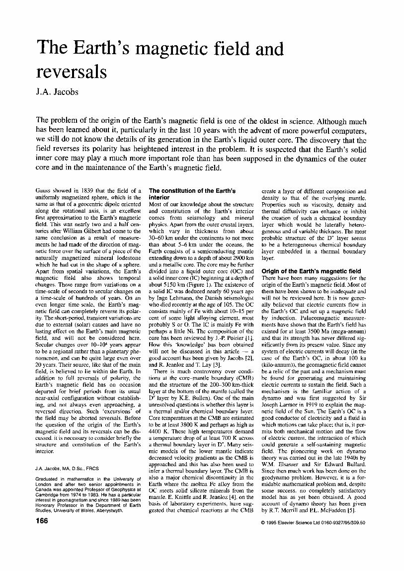
The constitution of the Earth’s interior Most of our knowledge about the structure and constitution of the Earth’s interior comes from seismology and mineral physics. Apart from the outer crustal layers, which vary in thickness from about 3@60 km under the continents to not more than about 5-6 km under the oceans, the Earth consists of a semiconducting mantle extending down to a depth of about 2900 km and a metallic core. The core may be further divided into a liquid outer core (OC) and a solid inner core (IC) beginning at a depth of about 5150 km (Figure 1). The existence of a solid IC was deduced nearly 60 years ago by Inge Lehmann, the Danish seismologist who died recently at the age of 105. The OC consists mainly of Fe with about 10-15 per cent of some light alloying element, most probably S or 0. The IC is mainly Fe with perhaps a little Ni. The composition of the core has been reviewed by J.-P Poirier [I]. How this ‘knowledge’ has been obtained will not be discussed in this article - a good account has been given by Jacobs [2], and R. Jeanloz and T. Lay [3].

There is much controversy over conditions at the core-mantle boundary (CMB) and the structure of the 20&300 km-thick layer at the bottom of the mantle (called the D” layer by K.E. Bullen). One of the main unresolved questions is whether this layer is a thermal and/or chemical boundary layer. Core temperatures at the CMB are estimated to be at least 3800 K and perhaps as high as 4400 K. These high temperatures demand a temperature drop of at least 700 K across a thermal boundary layer in D”. Many seismic models of the lower mantle indicate decreased velocity gradients as the CMB is approached and this has also been used to infer a thermal boundary layer. The CMB is also a major chemical discontinuity in the Earth where the molten Fe alloy from the OC meets solid silicate minerals from the mantle. E. Knittle and R. Jeanloz [4], on the basis of laboratory experiments, have suggested that chemical reactions at the CMB

create a layer of different composition and density to that of the overlying mantle. Properties such as viscosity, density and thermal diffusivity can enhance or inhibit the creation of such a chemical boundary layer which would be laterally heterogeneous and of variable thickness. The most probable structure of the D” layer seems to be a heterogeneous chemical boundary layer embedded in a thermal boundary layer.

Origin of the Earth’s magnetic field There have been many suggestions for the origin of the Earth’s magnetic field. Most of them have been shown to be inadequate and will not be reviewed here. It is now generally believed that electric currents flow in the Earth’s OC and set up a magnetic field by induction. Palaeomagnetic measurements have shown that the Earth’s field has existed for at least 3500 Ma (mega-annum) and that its strength has never differed significantly from its present value. Since any system of electric currents will decay (in the case of the Earth’s OC, in about 100 ka (kilo-annum)), the geomagnetic field cannot be a relic of the past and a mechanism must be found for generating and maintaining electric currents to sustain the field. Such a mechanism is the familiar action of a dynamo and was first suggested by Sir Joseph Larmor in 1919 to explain the magnetic field of the Sun. The Earth’s OC is a good conductor of electricity and a fluid in which motions can take place; that is, it per- mits both mechanical motion and the flow of electric current, the interaction of which could generate a self-sustaining magnetic field. The pioneering work on dynamo theory was carried out in the late 1940s by W.M. Elsasser and Sir Edward Bullard. Since then much work has been done on the geodynamo problem. However, it is a for- midable mathematical problem and, despite some success, no completely satisfactory model has as yet been obtained. A good account of dynamo theory has been given by R.T. Merrill and PL. McFadden [5].

0 1995 Elsevier Science Ltd 0160-9327/95/$09.50

Convection in the Earth’s outer core There have been a number of suggestions for the driving force of the geodynamo (see, for example, D. Gubbins and T.G. Masters [6]) and there is no reason to believe that only one mechanism operates. Non-linear interactions with a number of different processes giving rise to feedback are bound to lead to very complex behaviour and are typical of natural systems in a chaotic regime. It is possible that two different processes could act together to enhance the magnetic field or act in opposition to destroy the field.

There are two main contenders for the driving force - thermal convection and gravitational convection resulting from growth of the IC. Freezing of material at the inner core boundary (ICB) would separate a heavy fraction (mainly Fe). leaving behind a lighter fraction in the OC that would be buoyant, leading to compositionally driven convection. McFadden and Merrill [7] suggested that one of these two sources is responsible for generating the main field, the other producing instabilities that disrupt the field, leading on occasion to a reversal. It is possible that these two sources could at times change roles, depending on changing conditions at the CMB and ICB. Such dual behaviour of the two sources might explain the variable lengths of polarity intervals.

The same authors suggested two possible scenarios. In their first model, core motions, which drive the main magnetic field, result from gravitational convection associated with freezing of the OC at the ICB. In- stabilities are generated by heat loss at the CMB, cooler, more dense, cold blobs of fluid sinking and destabilizing the main convection. In their other model. core convection is due primarily to cooling at the CMB. The source of any instability is an occasional plume or hot blob given off at the ICB due to freezing of the OC with growth of the IC. A crucial question with either of these two models is the time-scale for a plume or blob to travel through the OC. A further question is how often are blobs/plumes released from the CMB/ICB and what is their success rate in traversing the whole OC?

H.H. Schloessin and J.A. Jacobs [8] had earlier suggested that reversals of the Earth’s magnetic field were the result of competing processes at the CMB and ICB. In their model of the evolution of the core, pressure freezing at the ICB and general cooling at the CMB lead to the formation of solid phases at both these boundaries, resulting in a solid IC and a lower mantle shell, which they identified with Bullen’s D” layer. Motions in the OC are caused and sustained by currents which offset density inhomogeneities at the advancing CMB and ICB. The concept of two competing processes in the OC was further investigated by P. Olson [9] who showed, from symmetry considerations. that the effects of IC growth tend to oppose and destabilize those generated by heat loss at the CMB.

Figure 1 Cross-section of the interior of the Earth. On this scale the crust canno: be seen.

H.K. Moffatt and D.E. Loper [lo] investigated the dynamics of a buoyant blob of fluid released from the ICB. They showed that when Lorenz and Coriolis forces are of comparable orders of magnitude, the disturb- ance remains localized in the neighbour- hood of the blob. They calculated the velocity and magnetic field associated with a given localized buoyancy distribution, and estimated that the rate of growth of the IC (assumed to be uniform) was = IO-ii m/s and, in further calculations, that the length- scale of an individual blob was in the range 0.1-100.0 km. On the assumption that the velocity is approximately uniform throughout the blob. they showed that the trajectory of the blob from the ICB to the CMB is a helix, indicating both a poleward component and a westward drift of the blob. The time rise of the blob from the ICB to the CMB was estimated to be = 100 a. Inherent in their theory is the presumption that the blobs will preserve their identity as they rise through the OC. M.G. St Pierre [ll] has carried out a numerical study of Moffatt and Loper’s model and found that the blobs will be greatly distorted after rising only a few

hundred kilometres from the ICB. They will be rapidly broken up into plate-like struc- tures elongated in the direction of rotation and of the prevalent magnetic field, giving rise to highly anistropic motions as foreseen earlier by S.I. Braginsky and V.P. Meitlis [12]. If substantiated, any large coherent buoyant structure in the Earth’s OC may be unstable.

Thermal convection in the OC has of late been thought to play a smaller role than compositional convection because of the low efficiency of a Camot cycle at core temperatures. However, B.A. Buffett et al. [ 131 have shown that thermal convection can contribute significantly to the energy budget of the geodynamo. A modest heat flux from the core in excess of that conducted down the adiabatic gradient is sufficient to power the geodynamo, even in the absence of compositional convection. The relative con- tributions of thermal and compositional convection to the geodynamo are largely determined by the magnitude of the heat flux from the core and the size of the IC. For plausible present-day values, compositional convection is responsible for - two-thirds

167

of the ohmic dissipation in the core and thermal convection for - one-third. Buffett et al. [ 131 point out that in the early Earth, when the IC was smaller and probably greater, thermal convection would have been the dominant source of energy for the geodynamo.

It is generally believed that the Earth’s core was formed very early in the Earth’s history (see, for example, C.J. All&gre et al. [14]). AllBgre et al. favour a slow continu- ing growth of the core, following a rapid initial growth - they estimate that 85 per cent of the core would have formed during the first N-200 Ma, and the remaining 15 per cent over the rest of geologic time. Rocks more than 3500 Ma old have been found which possess remanent magnetization, so that it is extremely likely that the Earth then had a molten OC about the same size as that at present. When the solid IC formed is a more difficult question, but if compositional convection in the OC plays a dominant role in driving the Earth’s dynamo, then a key question is when did the IC begin to form and what has been its rate of growth. D.J. Stevenson et al. [ 151 suggested that the mode of powering the geodynamo may have changed over geologic time. In the Earth’s early history, the magnetic field was generated by thermal convection with diminishing strength. After the onset of IC nucleation, the release of gravitational energy became the dominant source.

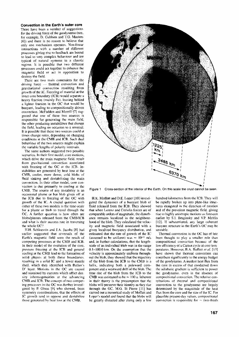
Buffett et al. [13] have investigated the time, formation and growth of the IC. Their method is based on global heat conservation, that is, the net heat flux from the OC is equated to that lost from the liquid OC together with that produced by the growth of the IC. They assume that temperatures throughout the OC (and hence the radius of the IC) are determined by the solidification temperature alone (treated as a function of pressure and hence of depth). Their solution depends on the magnitude and time depend- ence of the heat flux Q across the CMB. They take, as examples, probable maximum and minimum values of Q and obtain the time for the IC to grow to its present size as 1800 Ma and 4200 Ma respectively (Figure 2). Whether or not growth of the IC plays a significant role in initiating reversals, it is tempting to ascribe the long-term absence of reversals which have occurred on occasion (see later) to a change in the IC radius. This could be brought about by changing conditions at the CMB; for example, if the OC became colder, the melting point of Fe in the OC would be encountered further out and the radius of the IC would become larger.

The magnetization of rocks Most rock-forming minerals are non- magnetic, but all rocks show some magnetic properties due to the presence of various iron oxide and sulphide minerals making up only a few per cent of the rock. Information about the Earth’s magnetic field in the past comes from measurements

168

2000

5 1600 .

500

0 0 2 4 6

Time/lOga

Figure 2 Radius of the inner core (in km) measured from the time when solidification begins. Solutions are presented for three estimates for the net heat flux across the core-mantle boundary. The arrow indicates the current radius of the inner core. (After Buffett et al. [13].)

on igneous and sedimentary rocks which have acquired their magnetization by very different processes. Igneous rocks become magnetized as the different magnetic particles they contain cool below their Curie temperature (thermoremanent magnetization, TRM). When magnetic particles (erod- ed from pre-existing rock formations) fall through water, they will become aligned in the direction of the ambient magnetic field. This orientation may be preserved during the depositional process so that the resultant sediment acquires a remanent magnetization which is parallel to the field at the time of deposition (depositional remanent magnetization, DRM). If the carrier grains are free to rotate in the voids of the sediment matrix, they can follow the secular variation of the geomagnetic field and the magnetization they acquire will be that when they become locked into the sediment by consoli- dation (post-depositional remanent magnetization, PDRM).

In addition, a rock may acquire a remanent magnetization without heating if exposed to a magnetic field (isothermal remanent magnetization, IRM). This may be time-dependent, when it is referred to as viscous remanent magnetization (VRM). Finally, physicochemical changes may take place in rocks subsequent to their initial formation, and may involve crystallization of new magnetic mineral phases, and the rock may acquire an additional component of

magnetization. Such chemical remanent magnetization (CRM) may be important in sedimentary rocks as a result of lithification or chemical weathering. It is these very different processes by which rocks acquire their magnetization that compound the diffi- culties of interpreting the palaeomagnetic field.

In addition, there is the question of deter- mining the time of the acquisition of magnetization. Good estimates of the magnetic field may be obtained for volcanic rocks, but suffer from the fact that there is little chronological control. On the other hand, sedimentary rocks give reasonably good chronological control, but sedimentation rates are often too slow to allow detailed resolution of the field - only some (long- term) average can be obtained. Moreover, the amount of data for studying the behaviour of the Earth’s magnetic field in the past is quite small, and it is dangerous to infer properties of the field from a very limited record. Finally it must not be forgotten that the Earth’s magnetic field is generated in its core and the field we observe at the Earth’s surface has been filtered by passage through the overlying mantle.

Reversals of the Earth’s magnetic field Reversals of the Earth’s magnetic field were first found by B. Brunhes [16] in 1906 in lava flows from the Massif Central

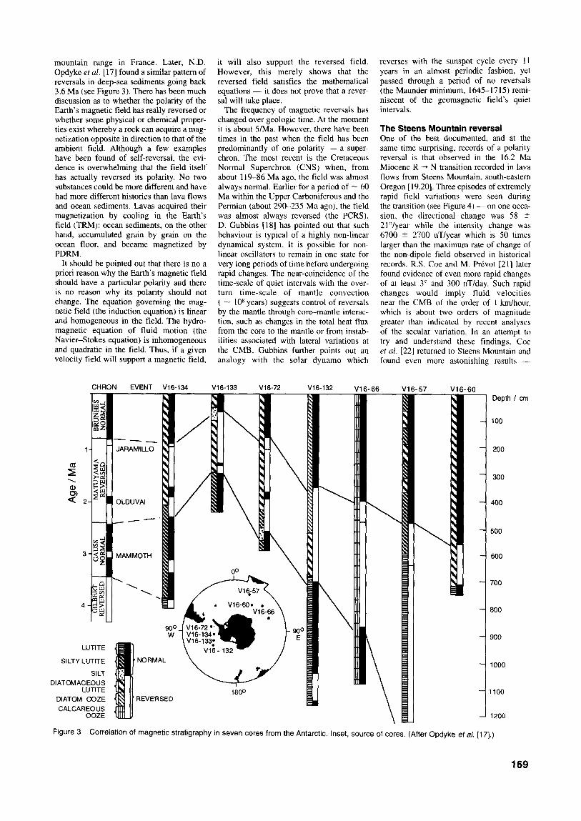
mountain range in France. Later, N.D. Opdyke et al. [ 171 found a similar pattern of reversals in deep-sea sediments going back 3.6 Ma (see Figure 3). There has been much discussion as to whether the polarity of the Earth’s magnetic field has really reversed or whether some physical or chemical properties exist whereby a rock can acquire a magnetization opposite in direction to that of the ambient field. Although a few examples have been found of self-reversal, the evidence is overwhelming that the field itself has actually reversed its polarity. No two substances could be more different and have had more different histories than lava flows and ocean sediments. Lavas acquired their magnetization by cooling in the Earth’s field (TRM): ocean sediments, on the other hand, accumulated grain by grain on the ocean floor, and became magnetized by PDRM.

It should be pointed out that there is no a priori reason why the Earth’s magnetic field should have a particular polarity and there is no reason why its polarity should not change. The equation governing the magnetic field (the induction equation) is linear and homogeneous in the field. The hydro- magnetic equation of fluid motion (the Navier-Stokes equation) is inhomogeneous and quadratic in the field. Thus, if a given velocity field will support a magnetic field,

it will also support the reversed field. However, this merely shows that the reversed field satisfies the mathematical equations - it does not prove that a reversal will take place.

The frequency of magnetic reversals has changed over geologic time. At the moment it is about 5/Ma. However, there have been times in the past when the field has been predominantly of one polarity - a superchron. The most recent is the Cretaceous Normal Superchron (CNS) when, from about 119-86 Ma ago, the field was almost always normal. Earlier for a period of - 60 Ma within the Upper Carboniferous and the Permian (about 290-235 Ma ago). the field was almost always reversed (the PCRS). D. Gubbins [18] has pointed out that such behaviour is typical of a highly non-linear dynamical system. It is possible for non- linear oscillators to remain in one state for very long periods of time before undergoing rapid changes. The near-coincidence of the time-scale of quiet intervals with the over- turn time-scale of mantle convection ( - IO8 years) suggests control of reversals by the mantle through core-mantle interaction, such as changes in the total heat flux from the core to the mantle or from instabilities associated with lateral variations at the CMB. Gubbins further points out an analogy with the solar dynamo which

CHRON EVENT V16-134 V16-133 VI 6-72 V16-132

SILTY LLJTITE

DIATOM OOZE

reverses with the sunspot cycle every 1 I years in an almost periodic fashion, yet passed through a period of no reversals (the Maunder minimum, 1645-1715) remi- niscent of the geomagnetic field’s quiet intervals.

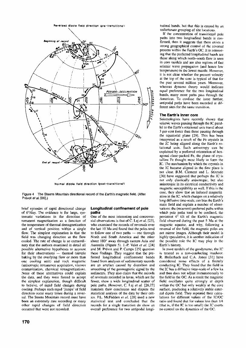
The Steens Mountain reversal One of the best documented, and at the same time surprising, records of a polarity reversal is that observed in the 16.2 Ma Miocene R --t N transition recorded in lava flows from Steens Mountain, south-eastern Oregon [ 19.201. Three episodes of extremely rapid field variations were seen during the transition (see Figure 4) - on one occasion, the directional change was 58 -C 2l”lyear while the intensity change was 6700 2 2700 nT/year which is 50 times larger than the maximum rate of change of the non-dipole field observed in historical records. R.S. Coe and M. Prevot [21] later found evidence of even more rapid changes of at least 3” and 300 nT/day. Such rapid changes would imply fluid velocities near the CMB of the order of 1 km/hour. which is about two orders of magnitude greater than indicated by recent analyses of the secular variation, In an attempt to try and understand these findings, Coe et nl. [22] returned to Steens Mountain and found even more astonishing results -

Depth I cm

100

200

300

400

600

Figure 3 Correlation of magnetic stratigraphy in seven cores from the Antarctic. Inset, source of cores. (After Opdyke et al. (171.)

169

Reverred dipole flrld dlrrctlon (Dre-trenslflona!)

Norms1 dipole (Iold dIrection (po8l-tronrlllonrl)

Figure 4 The Steens Mountain directional record of the Earth’s magnetic field. (After Pr&ot et al. [20].)

brief episodes of rapid directional change of 6”lday. The evidence is for large, sys- tematic variations in the direction of remanent magnetization as a function of the temperature of thermal demagnetization and of vertical position within a single flow. The simplest explanation is that the field was changing direction as the flow cooled. The rate of change is so extraordi- nary that the authors examined in detail all possible alternative hypotheses to account for their observations - thermal (simple baking by the overlying flow or more than one cooling unit) and rock magnetic (anisotropic remanence acquisition, viscous contamination, chemical remagnetization). None of these alternatives could explain the data, and they were forced to accept the simplest explanation, though difficult to believe, of rapid field changes during cooling. Perhaps such rapid ‘jumps’ of field direction occur many times during a reversal. The Steens Mountain record must have been an extremely rare recording or many other rapid changes of field direction occurred that were not recorded.

170

Longitudinal confinement of pole paths One of the most interesting and controver- sial observations is that of C. Laj et al. [23], who examined the records of reversals over the last 10 Ma and found that the poles tend to follow one of two paths - one through North and South America and the other about 180” away through eastern Asia and Australia (Figure 5). J.-P. Valet et al. [24] and M. Prevot and I? Camps [25] question these findings. They suggest that the preferred longitudinal confinement bands found from analyses of sedimentary records are an artefact caused by distortion and smoothing of the geomagnetic signal by the sediments. They also claim that the records of reversals recorded in lavas, which are far fewer, show a wide longitudinal scatter of pole paths. However, C. Laj er al. [26,27] maintain their conclusion and dispute the statistical analysis of the data by their crit- ics. PL. McFadden et al. [28] used a new statistical test and concluded that the records for a single transition do show an overall preference for two antipodal longi-

tudinal bands, but that this is caused by an unfortunate grouping of site locations.

If the concentration of transitional pole paths into two longitudinal bands is con- firmed, then it suggests that there exists a strong geographical control of the reversal process within the Earth’s OC. It is interesting that the preferred longitudinal bands are those along which north-south flow is seen in core models and are also regions of fast seismic wave propagation (and hence low temperature) in the lower mantle. However, it is not clear whether the present velocity at the top of the core is typical of that for the past several million years. Moreover, whereas dynamo theory would indicate equal preference for the two longitudinal bands, many more paths pass through the Americas. To confuse the issue further, antipodal paths have been recorded at different sites for the same transition.

The Earth’s inner core Seismologists have recently shown that seismic waves passing through the IC parallel to the Earth’s rotational axis travel about 3 per cent faster than those passing through the equatorial plane [29]. This has been interpreted as a result of the Fe crystals in the IC being aligned along the Earth’s rotational axis. Such anisotropy can be explained by a preferred orientation of hex- agonal close-packed Fe, the phase of crys- talline Fe thought most likely to form the IC. The mechanism by which the crystals in the IC became aligned in the first place is not clear. B.M. Clement and L. Stixrude [30] have suggested that perhaps the IC is not only elastically anisotropic, but also anisotropic in its electrical conductivity and magnetic susceptibility as well. If this is the case, they show that an induced magnetization in the IC, which changes on a relatively long diffusive time-scale, can bias the Earth’s main field and explain a number of observations: the (recurrent) preferred paths within which pole paths tend to be confined, the persistent 4” tilt of the Earth’s magnetic field observed during the past 5 Ma at the magnetic equator, and why, following a reversal of the field, the magnetic poles are not mirror images. Although their model is highly speculative, it is another indication of the possible role the IC may play in the Earth’s history.

In most models of the geodynamo, the IC is treated as a non-conducting insulator. R. Hollerbach and CA. Jones [31] have considered some effects of a finitely conducting IC. They found that the field in the IC has a diffusive time-scale of a few ka and thus does not adjust instantaneously to the field in the OC. As a result the magnetic field oscillates quite strongly at depth within the OC but only weakly at the core surface, producing a relatively stable external dipole field. They repeated their calculations for different values of the IC/OC ratio and found that for values less than 114 (that is, if the IC is too small) the IC exerts no control on the dynamics of the OC.

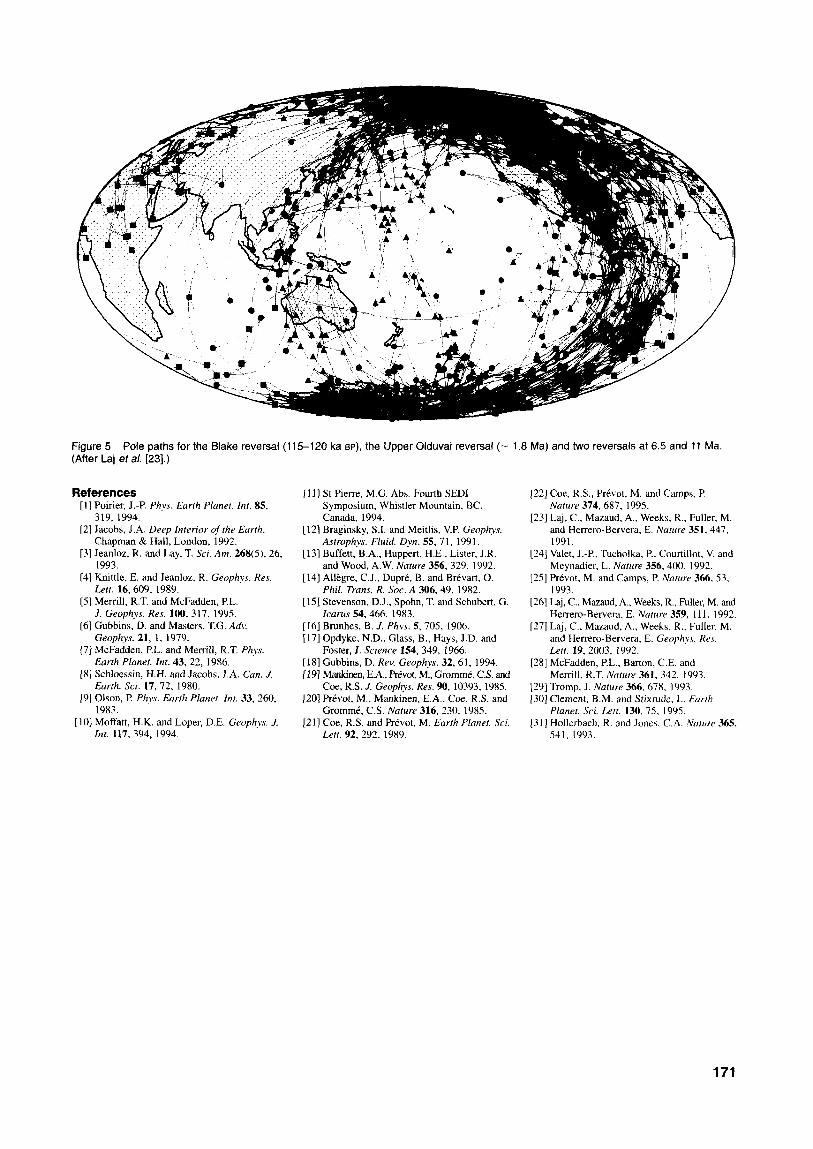
Figure 5 Pole paths for the Blake reversal (115-120 ka BP), the Upper Olduvai reversal (- 1.8 Ma) and two reversals at 6.5 and 11 Ma. (After Laj et al. [23].)

[22] Coe. R.S., PrCvot, M. and Camps, P. Nature 374. 687, 199.5.

[23] Laj, C., Mazaud, A., Weeks, R., Fuller, M. and Herrero-Bervera. E. Nature 351. 447, 1991.

[24] Valet, J.-P.. Tucholka, P., Courtillot, V. and Meynadier. L. Nature 356. 400. 1992.

[25] Prtvot, M. and Camps, P. Nature 366, 53, 1993.

References [II] St Pierre. M.G. Abs. Fourth SEDI [I] Poirier, J.-P. Phys. Earth Planet. Int. 85. Symposium, Whistler Mountain, BC.

319, 1994. Canada, 1994. [2] Jacobs, J.A. Deep Interior of the Earth. [ 121 Braginsky, S.I. and Meitlis, V.P. Geophys.

Chapman & Hall, London, 1992. Astrophys. Fluid. Dyz. 55. 7 1, 1991, [3] Jeanloz, R. and Lay, T. Sci. Am. 268(5), 26, [13] Buffett, B.A., Huppert, H.E., Lister, J.R.

1993. and Wood, A.W. Nature 356,329. 1992. [4] Knittle, E. and Jeanloz. R. Geophy. Rex [14] All&re, C.J., DuprC, B. and BrCvart. 0.

L&t. 16.609, 1989. Phil. Trans. R. Sot. A 306. 49. 1982. [5] Merrill, R.T. and McFadden, P.L. [1.5] Stevenson, D.J., Spohn, T. and Schubert. G.

.I. Geophys. Res. 100, 317, 1995. Icarus 54,466, 1983. [6] Gubbins, D. and Masters, T.G. Adv. [I61 Brunhes, B. J. Phys. 5,705, 1906.

Geophy. 21, 1, 1979. 1171 Opdyke, N.D.. Glass, B., Hays, J.D. and (71 McFadden, P.L. and Merrill, R.T. Phys. Foster, J. Science 154, 349, 1966.

Earth Planet. Int. 43, 22, 1986. [18] Gubbins, D. Rev. Geophys. 32,61, 1994. [S] Schloessin, H.H. and Jacobs, J.A. Can. 1. [ 191 Mankinen, E.A., Pr&ot, M., GrommC, C.S. and

Earrh. Sci. 17, 72, 1980. Coe, R.S. J. Geophys. Res. 90, 10393, 1985. [9] Olson, P. PJzw. Earth Planer. Int. 33, 260, 1201 Pr&vot, M., Mankinen, E.A.. Coe, R.S. and

1983. Grommt, C.S. Nature 316, 230, 1985. [ 10) Moffatt, H.K. and Loper, D.E. Geophw. .I. [21] Coe, R.S. and PrCvot, M. Earth P/met. Sri.

Int. 117. 394, 1994. Let?. 92. 292, 1989. 541.1993.

[26] Laj, C.. Mazaud, A., Weeks, R.. Fuller, M. and Herrero-Bervera. E. Nature 359, 111, 1992.

[27] Laj, C.. Mazaud, A., Weeks, R.. Fuller, M. and Herrero-Bervera, E. Geophys. Rrs. Len. 19, 2003, 1992.

[28] McFadden, P.L.. Barton, C.E. and Menill. R.T. Nature 361. 342. 1993.

[29] Tromp, J. Nafure 366. 678, 1993. [30] Clement, B.M. and Stixrude. L. Eurth

Planer. Sci. Mt. 130. 75. 1995. [31] Hollerbach. R. and Jones. C.A. N&we 365.

171

Documents

The Earth's magnetic field and reversals