1102

Russian Physics Journal, Vol. 56, No. 9, January, 2014 (Russian Original No. 9, September, 2013)

THE DIRAC EQUATION IN THE FRACTIONAL CALCULUS

V. S. Kirchanov UDC 530.1;536.75

Keywords: Dirac equation, fractional derivatives.

In [1, 2] the fractional Lagrangian method was used to obtain analogs of the Klein–Gordon equation for

fractional derivatives. In the present work this equation is obtained by the simple method of quantization of the energy invariant. Next, the standard path of factorization of the fractional Klein–Gordon equation is used to derive an analog of the Dirac equation in fractional derivatives. This equation can be useful in studies of the relativistic motion of an electron in fractal media [3]. Theoretical physics models with integrodifferentiation of fractional order were also considered in [4].

If we replace the energy and components of the momentum by fractional powers of the differentiation operators [5]

E it

α∂⎛ ⎞→ ⎜ ⎟∂⎝ ⎠ ( )0 1< α ≤ , k

kp i

x

β⎛ ⎞∂

→ − ⎜ ⎟∂⎝ ⎠ ( )0 1< β ≤ , 1, 2,3k = , (1)

in the energy invariant

( )22 2 2 2E p c mc= + , (2)

we obtain an analog of the Klein–Gordon equation in fractional differentials:

( )2 2 2

22 2

1 0m c xtc

αβ⎛ ⎞∂⎛ ⎞∇ − − ϕ =⎜ ⎟⎜ ⎟⎜ ⎟∂⎝ ⎠⎝ ⎠

, (3)

where 22 2

2

x y z

ββ ββ ∂ ∂ ∂⎛ ⎞⎛ ⎞ ⎛ ⎞∇ ≡ + +⎜ ⎟ ⎜ ⎟⎜ ⎟∂ ∂ ∂⎝ ⎠ ⎝ ⎠⎝ ⎠

is the Laplace operator in fractional derivatives, ( )xϕ is a scalar function,

( )0 1 2 3, , ,x x x x x= , 0 ,x ict= and 1 2 3, ,x x x y x z= = = . We introduce the fractional D'Alembert operator

2

22

1tc

ααβ β ∂⎛ ⎞≡ ∇ − ⎜ ⎟∂⎝ ⎠

(4)

and set 1c= = and α = β . Equation (3) then takes the form

Perm’ National Research Polytechnic University, Perm’, Russia, e-mail: Kichanv@rambler.ru. Translated from Izvestiya Vysshikh Uchebnykh Zavedenii, Fizika, No. 9, pp. 115–117, September, 2013. Original article submitted May 28, 2013.

1064-8887/14/5609-1102 ©2014 Springer Science+Business Media New York

1103

( ) ( )2 2 0xα −χ ϕ = . (5)

After factoring Eq. (5) we obtain an analog of the Dirac equation in fractional derivatives:

( ), 0x tx

α

μμ

⎡ ⎤⎛ ⎞∂⎢ ⎥γ − χ ψ =⎜ ⎟⎜ ⎟∂⎢ ⎥⎝ ⎠⎣ ⎦. (6)

Here μγ is the Pauli matrix, 1, 2,3,4μ = ,

1

2

3

4

ψ⎛ ⎞⎜ ⎟ψ⎜ ⎟ψ =⎜ ⎟ψ⎜ ⎟ψ⎝ ⎠

is the bispinor function, and 1

C

mcχ = =

λ is the inverse Compton

wavelength.

If we now act from the left with the operator x

α

νν

⎡ ⎤⎛ ⎞∂⎢γ + χ⎥⎜ ⎟∂⎢ ⎥⎝ ⎠⎣ ⎦

on Eq. (6), we should obtain the fractional

Klein–Gordon equation given by Eq. (5):

( )

( )2

, 0,

, 0,

x tx x

x tx x x x

αα

ν μν μ

α αα α

ν μ μ νν μ μ ν

⎡ ⎤⎡ ⎤ ⎛ ⎞⎛ ⎞∂ ∂⎢ ⎥⎢γ + χ⎥ γ − χ ψ =⎜ ⎟⎜ ⎟ ⎜ ⎟∂ ∂⎢ ⎥⎢ ⎥⎝ ⎠ ⎝ ⎠⎣ ⎦ ⎣ ⎦

⎡ ⎤⎛ ⎞ ⎛ ⎞⎛ ⎞ ⎛ ⎞∂ ∂ ∂ ∂⎢ ⎥γ γ + χγ − γ χ −χ ψ =⎜ ⎟ ⎜ ⎟⎜ ⎟ ⎜ ⎟⎜ ⎟ ⎜ ⎟∂ ∂ ∂ ∂⎢ ⎥⎝ ⎠ ⎝ ⎠⎝ ⎠ ⎝ ⎠⎣ ⎦

( )( ) ( )2

2 2 1 , 0.x tx x x

αα α

ν μν μ ν ν μν μ ν

⎡ ⎤⎛ ⎞⎛ ⎞ ⎛ ⎞∂ ∂ ∂⎢ ⎥γ − χ + − δ γ γ + γ γ ψ =⎜ ⎟⎜ ⎟ ⎜ ⎟⎜ ⎟∂ ∂ ∂⎢ ⎥⎝ ⎠ ⎝ ⎠⎝ ⎠⎣ ⎦

Since { } 2μ ν μ ν ν μ μνγ γ = γ γ + γ γ = δ , we obtain

( )2

2 2 , 0x tx

α

νν

⎡ ⎤⎛ ⎞∂⎢γ − χ ⎥ψ =⎜ ⎟∂⎢ ⎥⎝ ⎠⎣ ⎦

.

Thus, we have shown that each component μψ satisfies Eq. (5).

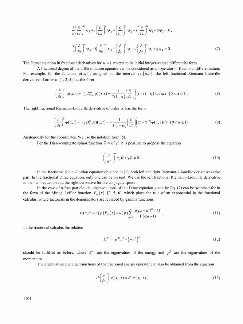
The Dirac equation in fractional derivatives given by Eq. (6) for a free particle in the Pauli representation can be written in the form of the following system:

1 4 4 3 1 0i i ic t x y z

αα α α∂ ∂ ∂ ∂⎛ ⎞⎛ ⎞ ⎛ ⎞ ⎛ ⎞− ψ − ψ − ψ − ψ + χψ =⎜ ⎟ ⎜ ⎟ ⎜ ⎟⎜ ⎟∂ ∂ ∂ ∂⎝ ⎠ ⎝ ⎠ ⎝ ⎠⎝ ⎠,

2 3 3 4 2 0i i ic t x y z

αα α α∂ ∂ ∂ ∂⎛ ⎞⎛ ⎞ ⎛ ⎞ ⎛ ⎞− ψ − ψ + ψ + ψ + χψ =⎜ ⎟ ⎜ ⎟ ⎜ ⎟⎜ ⎟∂ ∂ ∂ ∂⎝ ⎠ ⎝ ⎠ ⎝ ⎠⎝ ⎠,

1104

3 2 2 1 3 0i i ic t x y z

αα α α∂ ∂ ∂ ∂⎛ ⎞⎛ ⎞ ⎛ ⎞ ⎛ ⎞ψ + ψ + ψ + ψ + χψ =⎜ ⎟ ⎜ ⎟ ⎜ ⎟⎜ ⎟∂ ∂ ∂ ∂⎝ ⎠ ⎝ ⎠ ⎝ ⎠⎝ ⎠,

4 1 1 1 4 0i i ic t x y z

αα α α∂ ∂ ∂ ∂⎛ ⎞⎛ ⎞ ⎛ ⎞ ⎛ ⎞ψ + ψ − ψ − ψ + χψ =⎜ ⎟ ⎜ ⎟ ⎜ ⎟⎜ ⎟∂ ∂ ∂ ∂⎝ ⎠ ⎝ ⎠ ⎝ ⎠⎝ ⎠. (7)

The Diract equation in fractional derivatives for 1α = reverts to its initial integer-valued differential form. A fractional degree of the differentiation operator can be considered as an operator of fractional differentiation.

For example, for the function ( ),x tϕ , assigned on the interval [ ],t a b∈ , the left fractional Riemann–Liouville derivative of order α [1, 2, 5] has the form

( ) ( )( )

( )1, ( ) , ( ) ,1

t

a a ta

x t D x t t x dt t

αα −α+

∂ ∂⎛ ⎞ ⎛ ⎞ϕ = ϕ = − τ ϕ τ τ⎜ ⎟ ⎜ ⎟∂ Γ −α ∂⎝ ⎠ ⎝ ⎠∫ ( )0 1< α ≤ . (8)

The right fractional Riemann–Liouville derivative of order α has the form

( ) ( )( )

( )1, ( ) , ( ) ,1

b

b b tt

x t D x t t x dt t

αα −α−

∂ ∂⎛ ⎞ ⎛ ⎞ϕ = ϕ = − τ − ϕ τ τ⎜ ⎟ ⎜ ⎟∂ Γ −α ∂⎝ ⎠ ⎝ ⎠∫ ( )0 1< α ≤ . (9)

Analogously for the coordinates. We use the notation from [5]. For the Dirac-conjugate spinor function 0+ψ ≡ ψ γ it is possible to propose the equation

0x

α

μμ

∂⎛ ⎞ γ ψ + χψ =⎜ ⎟⎝ ⎠∂

. (10)

In the fractional Klein–Gordon equation obtained in [1], both left and right Riemann–Liouville derivatives take part. In the fractional Dirac equation, only one can be present. We use the left fractional Riemann–Liouville derivative in the main equation and the right derivative for the conjugate spinor.

In the case of a free particle, the eigensolutions of the Dirac equation given by Eq. (7) can be searched for in the form of the Mittag–Leffler function ( )E zα [2, 5, 6], which plays the role of an exponential in the fractional calculus, where factorials in the denominators are replaced by gamma functions:

( ) ( ) ( ) ( )( )0

[ ( ) / ],1

n

n

i px Etx t u p E z u pn

α∞

α=

−ψ = =

Γ α +∑ . (11)

In the fractional calculus the relation

( )22 2 2 2E p c mcα β= + (12)

should be fulfilled as before, where Eα are the eigenvalues of the energy and pβ are the eigenvalues of the momentum.

The eigenvalues and eigenfunctions of the fractional energy operator can also be obtained from the equation

( ) ( ), ,k ki x t E x tt

αα∂⎛ ⎞ ϕ = ϕ⎜ ⎟∂⎝ ⎠

, (13)

1105

the solution of which is given by the eigenfunction

( ) ( ) ( ) ( )( )0 0

0

[ ( ) / ],1

n

n

i Etx t u x E z u xn

α∞

α=

−ϕ = =

Γ α +∑ , (14)

where ( ) ( )0 , 0u x x t= ϕ = . Analogously, the solution of the equation for the fractional momentum

( ) ( ), ,k kk

i x t p x tx

ββ⎛ ⎞∂

− ϕ = ϕ⎜ ⎟∂⎝ ⎠ (15)

gives the eigenfunction

( ) ( ) ( ) ( )( )0 0

0

[ ( ) / ],

1

nk

kn

i pxx t v t E z v t

n

β∞

β=

ϕ = =Γ β +

∑ , (16)

where ( ) ( )0 0,v t x t= ϕ = . In conclusion, note that in the solution of the Dirac and Klein–Gordon equations it is necessary to use

regularized fractional derivatives to compensate for the integration constants [5, 6].

REFERENCES

1. E. M. Rabei, K. I. Nawfleh, R. S. Hijjawi, et al., J. Math. Appl., 327, 891 (2007). 2. V. V. Uchaikin, Method of Fractional Derivatives [in Russian], Artishok, Ul'yanovsk (2008). 3. A. V. Popov, Russ. Phys. J., 48, No. 9, 947–953 (2005). 4. V. E. Tarasov, Models of Theoretical Physics with Integrodifferentiation of Fractional Order [in Russian],

Regulyarnaya i Khaoticheskaya Dinamika, Izhevsk (2010). 5. S. G. Samko, A. A. Kilbas, and O. I. Marichev, Integrals and Derivatives of Fractional Order and Some of

Their Applications [in Russian], Nauka i Tekhnika, Minsk (1987). 6. V. S. Kirchanov, Russ. Phys. J., 49, No. 12, 1294–1300 (2006).