1

S03-2008 The Difference Between Predictive Modeling and Regression

Patricia B. Cerrito, University of Louisville, Louisville, KY

ABSTRACT Predictive modeling includes regression, both logistic and linear, depending upon the type of outcome variable. However, as the datasets are generally too large for a p-value to have meaning, predictive modeling uses other measures of model fit. Generally, too, there are enough observations so that the data can be partitioned into two or more datasets. The first subset is used to define (or train) the model. The second subset can be used in an iterative process to improve the model. The third subset is used to test the model for accuracy. The definition of “best” model needs to be considered as well. In a regression model, the “best” model is one that satisfies the criteria of uniform minimum variance unbiased estimator. In other words, it is only “best” in the class of unbiased estimators. As soon as the class of estimators is expanded, “best” no longer exists, and we must define the criteria that we will use to determine a “best” fit. There are several criteria to consider. For a binary outcome variable, we can use the misclassification rate. However, especially in medicine, misclassification can have different costs. A false positive error is not as costly as a false negative error if the outcome involves the diagnosis of a terminal disease. We will discuss the similarities and differences between the types of modeling. INTRODUCTION Regression has been the standard approach to modeling the relationship between one outcome variable and several input variables. Generally, the p-value is used as a measure of the adequacy of the model. There are other statistics, such as the r2 and the c-statistic (for logistic regression) that are presented, but are not usually considered as important. However, regression has limitations with large samples; all p-values are statistically significant with an effect size of virtually zero. For this reason, we need to be careful when interpreting the model. Instead, we can take a different approach. Because there are so many data values available, we can divide them and create holdout samples. Then, when using predictive modeling, we can use many different models simultaneously, and compare them to find the one that is the best. We can use the traditional regression, but also decision trees and neural network analysis. We can also combine different models. We can focus on accuracy of prediction rather than just identifying risk factors. There is still limited use of predictive modeling in medical research, with the exception of regression models. Most of the use of predictive modeling is fairly recent.(Sylvia et al., 2006) While most predictive models are used for examining costs (Powers, Meyer, Roebuck, & Vaziri, 2005), they can be invaluable in improving the quality of care.(Hodgman, 2008; Tewari et al., 2001; Weber & Neeser, 2006; Whitlock & Johnston, 2006) In this way, predictive modeling can be used to target the patients at highest risk for more intensive case management.(Weber & Neeser, 2006) It has also been used to examine workflow in the healthcare environment.(Tropsha & Golbraikh, 2007) Some studies focus on particular types of models such as neural networks.(Gamito & Crawford, 2004) In many cases, administrative (billing) data are used to identify patients who can benefit from interventions, and to identify patients who can benefit the most. Most of the use of predictive modeling is fairly recent. In particular, we will discuss some of the issues that are involved when using both linear and logistic regression. Regression requires an assumption of normality. The definition of confidence intervals, too, requires normality. However, most healthcare data are exponential or gamma. According to the Central Limit Theorem, the sample mean can be assumed normal if the sample is sufficiently large. However, if the distribution is exponential, just how large is large enough? If we use nonparametric models, we do not have to be as concerned with the actual population distribution. Also, we want to examine patient-level data rather than group-level data. That will mean that we will want to include information about patient condition in any regression model. Additional assumptions for regression are that the mean of the error term is equal to zero, and that the error term has equal variance for different levels of the input or independent variables. While the assumption of zero mean is almost always satisfied, the assumption of equal variance is not. Often, as the independent variables increase in value, the variance often increases as well. Therefore, modifications are needed to the variables, usually in the form of transformations, substituting the log of an independent variable for the variable itself. Transformations require considerable experience to use properly. In addition, the independent

2

variables are assumed to be independent of each other. While the model can tolerate some correlation between these variables, too much correlation will result in a poor model that cannot be used effectively on fresh data. A similar problem occurs if the independent variables have different range scales. If most of the variables are 0-1 indicator functions with patient’s age as a scale of 0-100, the value of age will completely dominate the regression equation. The variable scales should be standardized before the model is developed. Probably the most worrisome is the assumption that the error terms are identically distributed. In order for this assumption to be valid, we must assume the uniformity of data entry. That means that all providers must enter poorly defined values in exactly the same way. Unfortunately, such an assumption cannot possibly be valid. Consider, for example, the condition of “uncontrolled diabetes,” which is one coded patient condition. The term, “uncontrolled” is not defined. Therefore, the designation remains at the discretion of the provider to define the term. For this reason, different providers will define it differently. LOGISTIC REGRESSION We want to see if we can predict mortality in patients using a logistic regression model. There is considerable incentive to increase the number of positive indicators, called upcoding. The value,

25252221... XXX ααα +++

increases as the number of nonzero X’s increases. The greater this value, the greater the likelihood that it will cross the threshold value that predicts mortality. However, consider for a moment that just about every patient condition has a small risk of mortality. Once the threshold value is crossed, every patient with similar conditions are predicted to die. Therefore, the more patients who can be defined over the threshold value, the higher the predicted mortality rate, decreasing the difference between predicted and actual mortality. There is considerable incentive to upcode patient diagnoses to increase the likelihood of crossing this threshold vlaue. To simplify, we start with just one input variable to the logistic regression; the occurrence of pneumonia. Table 1 gives the chi-square table for the two variables. Table 1. Chi-square Table for Mortality by Pneumonia

Table of pneumonia by DIED

pneumonia DIED

Frequency Row Pct Col Pct

0 1

Total

0 743112998.2194.97

135419 1.79

81.02

7566548

1 39372892.545.03

31731 7.46

18.98

425459

Total 7824857 167150 7992007

Frequency Missing = 3041 Approximately 7% of the patients with pneumonia died compared to just under 2% generally. However, if we consider the classification table (Table 2) for a logistic regression with pneumonia as the input and mortality as the outcome variable, the accuracy rate is above 90% for any choice of threshold value of less than 1.0, where 100% of the values are to predict non-mortality. Therefore, even though patients with pneumonia are almost 4 times as likely to die compared to patients without pneumonia, pneumonia by itself is a poor predictor of mortality because of the rare occurrence.

3

Table 2. Classification Table for Logistic Regression

Classification Table

Correct Incorrect Percentages Prob Level

Event Non- Event

Event Non-Event

Correct Sensi-tivity

Speci- ficity

False POS

FalseNEG

0.920 782E4 0 167E3 0 97.9 100.0 0.0 2.1 .

0.940 743E4 31731 135E3 394E3 93.4 95.0 19.0 1.8 92.5

0.960 743E4 31731 135E3 394E3 93.4 95.0 19.0 1.8 92.5

0.980 743E4 31731 135E3 394E3 93.4 95.0 19.0 1.8 92.5

1.000 0 167E3 0 782E4 2.1 0.0 100.0 . 97.9 We now add a second patient diagnosis to the regression. Table 3 gives the chi-square table for pneumonia and septicemia. Table 3. Chi-square Table for Pneumonia and Septicemia

Controlling for septicemia=0 Controlling for septicemia=1

pneumonia Died Total DIED Total

Frequency Row Pct Col Pct

0 1 0 1

0 730772698.6095.20

103759 1.40

82.65

7411485

12340379.5883.06

3166020.4276.09

155063

1 36855394.424.80

21783 5.58

17.35

390336

2517571.6816.94

994828.3223.91

35123

Total 7676279 125542 7801821 148578 41608 190186 Of the patients with septicemia only (pneumonia=0), 20% died, increasing to 28% with both septicemia and pneumonia. For patients without septicemia but with pneumonia, 5% died. The classification table for the logistic regression is given in Table 4. Table 4. Classification Table for Logistic Regression With Pneumonia and Septicemia

Classification Table

Correct Incorrect Percentages Prob Level

Event Non- Event

Event Non-Event

Correct Sensi-tivity

Speci- ficity

False POS

FalseNEG

0.580 782E4 0 167E3 0 97.9 100.0 0.0 2.1 .

0.600 78E5 9948 157E3 25175 97.7 99.7 6.0 2.0 71.7

0.620 78E5 9948 157E3 25175 97.7 99.7 6.0 2.0 71.7

0.640 78E5 9948 157E3 25175 97.7 99.7 6.0 2.0 71.7

0.660 78E5 9948 157E3 25175 97.7 99.7 6.0 2.0 71.7

0.680 78E5 9948 157E3 25175 97.7 99.7 6.0 2.0 71.7

0.700 78E5 9948 157E3 25175 97.7 99.7 6.0 2.0 71.7

0.720 78E5 9948 157E3 25175 97.7 99.7 6.0 2.0 71.7

4

Classification Table

Correct Incorrect Percentages Prob Level

Event Non- Event

Event Non-Event

Correct Sensi-tivity

Speci- ficity

False POS

FalseNEG

0.740 78E5 9948 157E3 25175 97.7 99.7 6.0 2.0 71.7

0.760 78E5 9948 157E3 25175 97.7 99.7 6.0 2.0 71.7

0.780 78E5 9948 157E3 25175 97.7 99.7 6.0 2.0 71.7

0.800 78E5 9948 157E3 25175 97.7 99.7 6.0 2.0 71.7

0.820 78E5 9948 157E3 25175 97.7 99.7 6.0 2.0 71.7

0.840 768E4 41608 126E3 149E3 96.6 98.1 24.9 1.6 78.1

0.860 768E4 41608 126E3 149E3 96.6 98.1 24.9 1.6 78.1

0.880 768E4 41608 126E3 149E3 96.6 98.1 24.9 1.6 78.1

0.900 768E4 41608 126E3 149E3 96.6 98.1 24.9 1.6 78.1

0.920 768E4 41608 126E3 149E3 96.6 98.1 24.9 1.6 78.1

0.940 768E4 41608 126E3 149E3 96.6 98.1 24.9 1.6 78.1

0.960 731E4 63391 104E3 517E3 92.2 93.4 37.9 1.4 89.1

0.980 731E4 63391 104E3 517E3 92.2 93.4 37.9 1.4 89.1

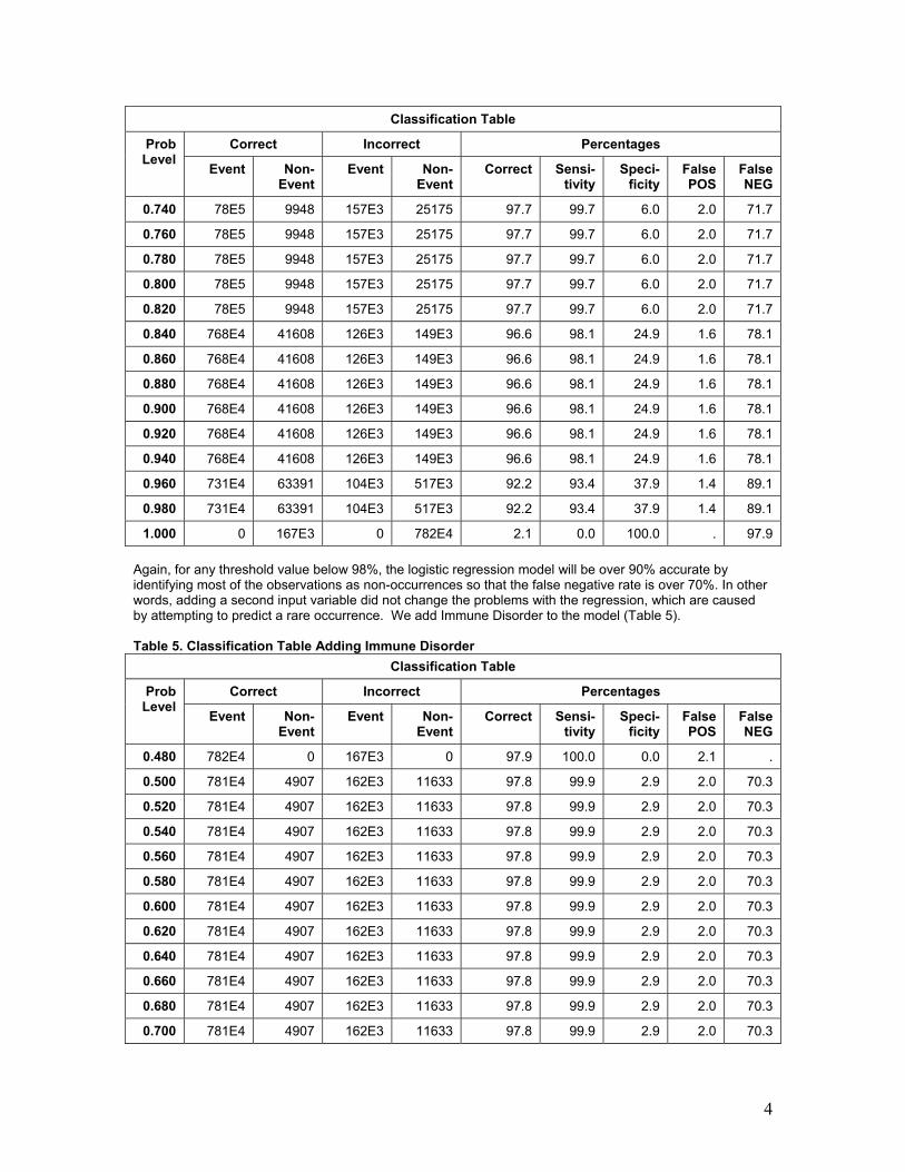
1.000 0 167E3 0 782E4 2.1 0.0 100.0 . 97.9 Again, for any threshold value below 98%, the logistic regression model will be over 90% accurate by identifying most of the observations as non-occurrences so that the false negative rate is over 70%. In other words, adding a second input variable did not change the problems with the regression, which are caused by attempting to predict a rare occurrence. We add Immune Disorder to the model (Table 5). Table 5. Classification Table Adding Immune Disorder

Classification Table

Correct Incorrect Percentages Prob Level

Event Non- Event

Event Non-Event

Correct Sensi-tivity

Speci- ficity

False POS

FalseNEG

0.480 782E4 0 167E3 0 97.9 100.0 0.0 2.1 .

0.500 781E4 4907 162E3 11633 97.8 99.9 2.9 2.0 70.3

0.520 781E4 4907 162E3 11633 97.8 99.9 2.9 2.0 70.3

0.540 781E4 4907 162E3 11633 97.8 99.9 2.9 2.0 70.3

0.560 781E4 4907 162E3 11633 97.8 99.9 2.9 2.0 70.3

0.580 781E4 4907 162E3 11633 97.8 99.9 2.9 2.0 70.3

0.600 781E4 4907 162E3 11633 97.8 99.9 2.9 2.0 70.3

0.620 781E4 4907 162E3 11633 97.8 99.9 2.9 2.0 70.3

0.640 781E4 4907 162E3 11633 97.8 99.9 2.9 2.0 70.3

0.660 781E4 4907 162E3 11633 97.8 99.9 2.9 2.0 70.3

0.680 781E4 4907 162E3 11633 97.8 99.9 2.9 2.0 70.3

0.700 781E4 4907 162E3 11633 97.8 99.9 2.9 2.0 70.3

5

Classification Table

Correct Incorrect Percentages Prob Level

Event Non- Event

Event Non-Event

Correct Sensi-tivity

Speci- ficity

False POS

FalseNEG

0.720 781E4 4907 162E3 11633 97.8 99.9 2.9 2.0 70.3

0.740 776E4 21322 146E3 65076 97.4 99.2 12.8 1.8 75.3

0.760 775E4 26363 141E3 78618 97.3 99.0 15.8 1.8 74.9

0.780 775E4 26363 141E3 78618 97.3 99.0 15.8 1.8 74.9

0.800 775E4 26363 141E3 78618 97.3 99.0 15.8 1.8 74.9

0.820 775E4 26363 141E3 78618 97.3 99.0 15.8 1.8 74.9

0.840 775E4 26363 141E3 78618 97.3 99.0 15.8 1.8 74.9

0.860 775E4 26363 141E3 78618 97.3 99.0 15.8 1.8 74.9

0.880 775E4 26363 141E3 78618 97.3 99.0 15.8 1.8 74.9

0.900 768E4 41608 126E3 149E3 96.6 98.1 24.9 1.6 78.1

0.920 757E4 51297 116E3 258E3 95.3 96.7 30.7 1.5 83.4

0.940 757E4 51297 116E3 258E3 95.3 96.7 30.7 1.5 83.4

0.960 757E4 51297 116E3 258E3 95.3 96.7 30.7 1.5 83.4

0.980 634E4 103E3 64219 149E4 80.6 81.0 61.6 1.0 93.5

1.000 0 167E3 0 782E4 2.1 0.0 100.0 . 97.9 The problem still persists, and will continue to persist regardless of the number of input variables. We need to change the sample size so that the group sizes are close to equal.

PREDICTIVE MODELING IN SAS ENTERPRISE MINER Figure 1 gives a diagram of a predictive model in SAS Enterprise Miner. Enterprise Miner includes the standard types of regression, artificial neural networks, and decision trees. The regression model will choose linear or logistic automatically, depending upon the type of outcome variable. Figure 1 shows that many different models can be used. Once defined, the models are compared and the optimal model chosen based upon pre-selected criteria. Then, additional data can be scored so that patients, in this example, at high risk for adverse events can be identified for more aggressive treatment. The purpose of the partition node in Figure 1 is to divide the data into training, validation, and testing subsets, by default, a 40/30/30 split in the data. Usually, the datasets are large enough that such a partitioning is possible. The training set is used to define the model; the testing set is a holdout sample used as fresh data to test the accuracy of the model. The validation set is not needed for regression; it is needed for neural networks and any model that is defined iteratively. The model is examined on the validation set, and adjustments are made to the model if necessary. This process is repeated until no more changes are necessary.

6

Figure 1. Predictive Modeling of Patient Outcomes

For predicting a rare occurrence, one more node is added to the model in Figure 1, the sampling node (Figure 2). This node uses all of the observations with the rare occurrence, and then takes a random sample of the remaining data. While the sampling node can use any proportional split, we recommend a 50:50 split. Figure 3 shows how the defaults are modified in the sampling node of SAS Enterprise Miner to make predictions.

7

Figure 2. Addition of Sampling Node

8

Figure 3. Change to Defaults in Sampling Node

The first arrow indicates that the sampling is stratified, and the criterion is level based. The rarest level (in this case, mortality) is sampled so that it will consist of half (50% sample proportion) of the sample. Consider the problem of predicting mortality that was discussed in the previous section on logistic regression. We use just the same three patient diagnoses of pneumonia, septicemia, and immune disorder that we used previously. However, in this case, we use the sampling node to get a 50/50 split in the data. We use all of the models depicted in Figure 1. According to the model comparison, the rule induction provides the best fit, using the misclassification rate as the measure of “best”. We first look at the regression model, comparing the results to those in the previous chapter when a 50/50 split was not performed. The overall misclassification rate is 28%, with the divisions as shown in Table 6. Table 6. Misclassification in Regression Model Target Outcome Target Percentage Outcome Percentage Count Total Percentage Training Data 0 0 67.8 80.1 54008 40.4 1 0 32.2 38.3 25622 19.2 0 1 23.8 19.2 12852 9.6 1 1 76.3 61.7 41237 30.8 Validation Data 0 0 67.7 80.8 40498 40.4 1 0 32.3 38.5 19315 19.2 0 1 23.8 19.2 9646 9.6 1 1 76.2 61.5 30830 30.7

9

Note that the misclassification becomes more balanced between false positives and false negatives with a 50/50 split in the data. The model gives heavier weight to false positives than it does to false negatives. We also want to examine the decision tree model. While it is not the most accurate model, it is one that clearly describes the rationale behind the predictions. This tree is given in Figure 4. The tree shows that the first split occurs on the variable, Septicemia. Patients with Septicemia are more likely to suffer mortality compared to patients without Septicemia. As shown in the previous chapter, the Immune Disorder has the next highest level of mortality followed by Pneumonia. Figure 4. Decision Tree Results

Since rule induction is identified as the best model, we examine that one next. The misclassification rate is only slightly smaller compared to the regression model. Table 7 gives the classification table. Table 7. Misclassification in Rule Induction Model Target Outcome Target Percentage Outcome Percentage Count Total Percentage Training Data 0 0 67.8 80.8 54008 40.4 1 0 32.2 38.3 25622 19.2 0 1 23.8 19.2 12852 9.6 1 1 76.3 61.7 41237 30.8 Validation Data

10

Target Outcome Target Percentage Outcome Percentage Count Total Percentage Training Data 0 0 67.7 80.8 40498 40.4 1 0 32.3 38.5 19315 19.2 0 1 23.8 19.2 9646 9.6 1 1 76.2 61.5 30830 30.7 The results look virtually identical to those in Table 6. For this reason, the regression model, although not defined as the best, can be used to predict outcomes when only these three variables are used. The similarities in the models can also be visualized in the ROC (received-operating curve) that graphs the sensitivity versus one minus the specificity (Figure 5). The curves for rule induction and regression are virtually the same. Figure 5. Comparison of ROC Curves

MANY VARIABLES IN LARGE SAMPLES There can be hundreds if not thousands of variables collected for each patient. These are far too many to include in any predictive model. The use of too many variables can cause the model to over-fit the results, inflating the outcomes. Therefore, there needs to be some type of variable reduction method. In the past, factor analysis has been used to reduce the set of variables prior to modeling the data. However, there is now a more novel method available (Figure 6). In our example, there are many additional variables that can be considered in this analysis. Therefore, we use the variable selection technique to choose the most relevant. We first use the decision tree followed by regression, and then regression followed by the decision tree.

11

Figure 6. Variable Selection

Using the decision tree to define the variables, Figure 7 shows the ones that remain for the modeling. Figure 7. Decision Tree Variables

This tree shows that age, length of stay, having septicemia, immune disorder, and total charges are related to mortality. The remaining variables have been rejected from the model. The rule induction is the best model, and the misclassification rate decreases to 22% with the added variables. The ROC curve looks considerably improved (Figure 8).

12

Figure 8. ROC Curves for Models Following Decision Tree

The ROC curve is much higher compared to that in Figure 5. If we use regression to perform the variable selection, the results remain the same. In addition, a decision tree is virtually the same when it follows the regression compared to when it precedes (Figure 9). Figure 9. Decision Tree Following Regression

The above example only used three possible diagnosis codes. We want to expand upon the number of diagnosis codes, and also to use a number of procedure codes. In this example, we restrict our attention to

13

patients with a primary diagnosis of COPD (chronic obstructive pulmonary disease resulting primarily from smoking). There are approximately 245,000 patients in the NIS dataset. Table 8 gives the list of diagnosis codes used; Table 9 gives a list of procedure codes used as well. Table 8. Diagnosis Codes Used to Predict Mortality Condition ICD9 Codes Acute myocardial infarction

410, 412

Congestive heart failure

428

Peripheral vascular disease

441,4439,7854,V434

Cerebral vascular accident

430-438

Dementia 290 Pulmonary disease

490,491,492,493,494,495,496,500,501,502,503,504,505

Connective tissue disorder

7100,7101,7104,7140,7141,7142,7148,5171,725

Peptic ulcer 531,532,533,534 Liver disease 5712,5714,5715,5716 Diabetes 2500,2501,2502,2503,2507 Diabetes complications

2504,2505,2506

Paraplegia 342,3441 Renal disease 582,5830,5831,5832,5833,5835,5836,5837,5834,585,586,588 Cancer 14,15,16,17,18,170,171,172,174,175,176,179,190,191,193, 194,1950,1951,1952,

1953,1954,1955,1958,200,201,202,203, 204,205,206,207,208 Metastatic cancer

196,197,198,1990,1991

Severe liver disease

5722,5723,5724,5728

HIV 042,043,044 Table 9. Procedure Codes Used to Predict Mortality

14

pr Procedure Translation Frequency Percent

9904 Transfusion of packed cells 17756 7.05

3893 Venous catheterization, not elsewhere classified 16142 6.41

9671 Continuous mechanical ventilation for less than 96 consecutive hours 10528 4.18

3324 Closed [endoscopic] biopsy of bronchus 8315 3.30

9672 Continuous mechanical ventilation for 96 consecutive hours or more 8243 3.27

3491 Thoracentesis 8118 3.22

3995 Hemodialysis 8083 3.21

9604 Insertion of endotracheal tube 7579 3.01

9921 Injection of antibiotic 6786 2.69

9394 Respiratory medication administered by nebulizer 6309 2.50

8872 Diagnostic ultrasound of heart 5419 2.15

4516 Esophagogastroduodenoscopy [EGD] with closed biopsy 4894 1.94

9390 Continuous positive airway pressure 4667 1.85

3327 Closed endoscopic biopsy of lung 3446 1.37

8741 Computerized axial tomography of thorax 3417 1.36

4513 Other endoscopy of small intestine 3277 1.30 If we perform standard logistic regression without stratified sampling, the false positive rate remains small (approximately 3-4%), but with a high false negative rate (minimized at 38%). Given the large dataset, almost all of the input variables are statistically significant. The percent agreement is 84% and the ROC curve looks fairly good (Figure 10). Figure 10. ROC Curve for Traditional Logistic Regression

15

If we perform predictive modeling, the accuracy rate drops to 75%, but the false negative rate is considerably improved. Figure 11 gives the ROC curve from predictive modeling. Figure 11. ROC From Predictive Modeling

CHANGE IN SPLIT IN THE DATA All of the analyses in the previous section assumed a 50/50 split between mortality and non-mortality. We want to look at the results if mortality composes only 25% of the data, and 10% of the data. Table 10 gives the regression classification breakdown for a 25% sample; Table 11 gives the breakdown for a 10% sample. Table 10. Misclassification Rate for a 25% Sample Target Outcome Target Percentage Outcome Percentage Count Total Percentage Training Data 0 0 80.4 96.6 10070 72.5 1 0 19.6 70.9 2462 17.7 0 1 25.6 3.3 348 2.5 1 1 74.4 29.1 1010 7.3 Validation Data 0 0 80.2 97.1 7584 72.8 1 0 19.8 71.7 1870 17.9 0 1 23.7 2.9 229 2.2 1 1 76.2 28.2 735 7.0 Note that the ability to classify mortality accurately is decreasing with the decrease of the split; almost all of the observations are classified as non-mortality. The decision tree (Figure 12) is considerably different from that in Figure 9 with a 50/50 split. Now, the procedure of Esophagogastroduodenoscopy gives the first leaf of the tree. Figure 12. Decision Tree for 25/75 Split in the Data

16

Table 11. Misclassification Rate for a 10% Sample Target Outcome Target Percentage Outcome Percentage Count Total Percentage Training Data 0 0 91.5 99.3 31030 89.4 1 0 8.5 83.5 2899 8.3 0 1 27.3 0.7 216 0.6 1 1 72.6 16.5 574 1.6 Validation Data 0 0 91.5 99.2 23265 89.3 1 0 8.4 82.4 2148 8.2 0 1 27.8 0.7 176 0.7 1 1 72.2 17.5 457 1.7 Note that the trend shown in the 25% is even more exaggerated in the 10% sample. Figure 13 shows that the decision tree has changed yet again. It now includes the procedure of continuous positive airway pressure and the diagnosis of congestive heart failure. AT a 1% sample, the misclassification becomes even more disparate. Figure 13. Decision Tree for 10% Sample

17

ADDITION OF WEIGHTS FOR DECISION MAKING In most medical studies, a false negative is more costly to the patient compared to a false positive. This occurs because a false positive generally leads to more invasive tests; however, a false negative means that a potentially life-threatening illness will go undiagnosed, and hence, untreated. Therefore, we can weight a false negative at higher cost, and then change the definition of a “best” model to one that minimizes costs. The problem is to determine which costs to use. The best thing to do is to experiment with magnitudes of difference in cost between the false positive and false negative to see what happens. At a 1:1 ratio, the best model is still based upon the misclassification rate. A change to a 5:1 ratio indicates that a false negative is five times as costly compared to a false positive. A 10:1 ratio makes it ten times as costly. We need to determine if changes to this ratio result in changes to the optimal model.

INTRODUCTION TO LIFT Lift allows us to find the patients at highest risk for occurrence, and with the greatest probability of accurate prediction. This is especially important since these are the patients we would want to take the greatest care for.

Using lift, true positive patients with highest confidence come first, followed by positive patients with lower confidence. True negative cases with lowest confidence come next, followed by negative cases with highest confidence. Based on that ordering, the observations are partitioned into deciles, and the following statistics are calculated:

18

• The Target density of a decile is the number of actually positive instances in that decile divided by the total number of instances in the decile.

• The Cumulative target density is the target density computed over the first n deciles. • The lift for a given decile is the ratio of the target density for the decile to the target density over all

the test data. • The Cumulative lift for a given decile is the ratio of the cumulative target density to the target

density over all the test data.

Given a lift function, we can decide on a decile cutpoint so that we can predict the high risk patients above the cutpoint, and predict the low risk patients below a second cutpoint, while failing to make a definite prediction for those in the center. In that way, we can dismiss those who have no risk, and aggressively treat those at highest risk. Lift allows us to distinguish between patients without assuming a uniformity of risk. Figure 14 shows the lift for the testing set when we use just the three input variables of pneumonia, septicemia, and immune disorder.

Figure 14. Lift Function for Three-Variable Input

Random chance is indicates by the lift value of 1.0; values that are higher than 1.0 indicate that the observations are more predictable compared to random chance. In this example, 40% of the patient records have a higher level of prediction than just chance. Therefore, we can concentrate on these 4 deciles of patients. If we use the expanded model that includes patient demographic information plus additional diagnosis and procedure codes for COPD, we get the lift shown in Figure 15. The model can now predict the first 5 deciles of patient outcomes.

Figure 15. Lift Function for Complete Model

Therefore, we can predict accurately those patients most at risk for death; we can determine which patients can benefit from more aggressive treatment to reduce the likelihood that this outcome will occur. DISCUSSION Given large datasets and the presence of outliers, the traditional statistical methods are not always applicable or meaningful. Assumptions can be crucial to the applicability of the model, and assumptions are

19

not always carefully considered. The assumptions of a normal distribution and uniformity of data entry are crucial and need to be considered carefully. The data may not give high levels of correlation, and regression may not always be the best way to measure associations. It must also be remembered that associations in the data as identified in regression models do not demonstrate cause and effect. CONTACT INFORMATION

Patricia Cerrito Department of Mathematics University of Louisville Louisville, KY 40292 502-852-6010 502-852-7132 (fax) pcerrito@louisville.edu http://stores.lulu.com/dataservicesonline

SAS and all other SAS Institute Inc. product or service names are registered trademarks or trademarks of SAS Institute Inc. in the USA and other countries. ® indicates USA registration. Other brand and product names are trademarks of their respective companies.