The Cyclicality of International Public Sector Borrowing ...repec.graduateinstitute.ch/pdfs/Working_papers/HEIDWP17-2017.pdf · each other leading to a “when it rains it pours”

Graduate Institute of International and Development Studies

International Economics Department

Working Paper Series

Working Paper No. HEIDWP17-2017

The Cyclicality of International Public Sector Borrowing inDeveloping Countries: Does the Lender Matter?

Arturo J. GalindoInter-American Development Bank

Ugo PanizzaThe Graduate Institute Geneva and CEPR

Chemin Eugene-Rigot 2P.O. Box 136

CH - 1211 Geneva 21Switzerland

c©The Authors. All rights reserved. Working Papers describe research in progress by the author(s) and are published toelicit comments and to further debate. No part of this paper may be reproduced without the permission of the authors.

1

The Cyclicality of International Public Sector Borrowing in Developing

Countries: Does the Lender Matter?

Arturo J. Galindo

Inter-American Development Bank

Ugo Panizza*

The Graduate Institute Geneva & CEPR

Abstract

The paper shows that international government borrowing from multilateral development

banks is countercyclical while international government borrowing form private sector

lenders is procyclical. The countercyclicality of official lending is mostly driven by the

behavior of the World Bank (borrowing from regional development banks tends to be

acyclical). The paper also shows that official sector lending to Latin America and East

Asia is more countercyclical than official lending to other regions. Private sector lending

is instead procyclical in all developing regions. While the cyclicality of official lending

does not depend on domestic or international conditions, private lending becomes

particularly procyclical in periods of limited global capital flows. By focusing on both

borrowers and lenders’ heterogeneity the paper shows that the cyclical properties of

international government debt are mostly driven by credit supply shocks. Demand

factors appear to be less important drivers of procyclical international government

borrowing. The paper’s focus on supply and demand factors is different from the

traditional push and pull classification, as push and pull factors could affect both the

demand and the supply of international government debt.

Keywords: International Government Debt; Capital Flows, Fiscal Policy; International

Financial Institutions

JEL Codes: E62; F34; F32

* We would like to thank Carola Alvarez, Miguel Castilla, Alberto Carrasquilla, Eduardo Cavallo,

Augusto de la Torre, and seminar participants at the Inter-American Development Bank for useful

comments and suggestions, and Alen Mulabdic for help with the construction of the external

demand shock. The usual caveats apply.

2

1 Introduction

This paper studies the cyclical properties of international government debt by focusing

on the heterogeneous behavior of different types of lenders and by exploring over-time

and cross-sectional borrower heterogeneity.

The paper is related to a large literature that studies the cyclicality of capital

flows to developing and emerging market countries and to an equally large literature that

studies the cyclical behavior of fiscal policy in advanced and developing economies. The

consensus is that in developing and emerging market countries both capital flows and

fiscal policy tend to be procyclical and that these two forms of procyclicality reinforce

each other leading to a “when it rains it pours” phenomenon (Kaminsky, Reinhart, and

Végh, 2004).1 These findings are in contrast with standard models which predict that

both international capital flows and fiscal policy should be countercyclical.2

The literature on the drivers of procyclical capital flows to developing countries

has focused on the differences between pull (capital flows are driven by attractive

domestic conditions in developing countries) and push factors (capital flows are pushed

by low returns in advanced economies) and concluded that push factors are the key

drivers of portfolio flows.3 Two classic papers in this line of research are Calvo,

Leiderman, and Reinhart (1993) and Fernandez-Arias (1996). More recent work includes

Fratzscher (2011) and Forbes and Warnock (2012).

The literature on the cyclicality of fiscal policy has instead emphasized two

types of explanations for procyclicality. The first class of explanations focuses on capital

market imperfections which lead to a situation in which, like Mark Twain’s proverbial

banker, international financiers stand ready to lend an umbrella when the sun is shining

but want it back as soon as it starts raining. According to this view, procyclicality is

driven by that fact that developing countries lack access to international credit during

recessions (Gavin and Perotti, 1997). An alternative class of explanations concentrates

on political failures and shows that fiscal procyclicality may arise from political pressure

1 For a contrarian view on the procyclicality of fiscal policy in developing countries see

Jaimovich and Panizza (2007). 2 The former helps smoothing consumption by transferring income from good to bad states of the

world and the latter can either minimize tax distortions (Barro, 1979) or stabilize the economic

cycle as in the typical Keynesian countercyclical policy. 3 However, Cerutti, Claessens, and Puy (2015) show that the importance of push factors varies

across types of flows.

3

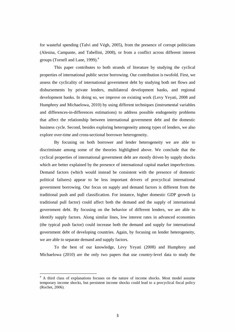
for wasteful spending (Talvi and Végh, 2005), from the presence of corrupt politicians

(Alesina, Campante, and Tabellini, 2008), or from a conflict across different interest

groups (Tornell and Lane, 1999).4

This paper contributes to both strands of literature by studying the cyclical

properties of international public sector borrowing. Our contribution is twofold. First, we

assess the cyclicality of international government debt by studying both net flows and

disbursements by private lenders, multilateral development banks, and regional

development banks. In doing so, we improve on existing work (Levy Yeyati, 2008 and

Humphrey and Michaelowa, 2010) by using different techniques (instrumental variables

and differences-in-differences estimations) to address possible endogeneity problems

that affect the relationship between international government debt and the domestic

business cycle. Second, besides exploring heterogeneity among types of lenders, we also

explore over-time and cross-sectional borrower heterogeneity.

By focusing on both borrower and lender heterogeneity we are able to

discriminate among some of the theories highlighted above. We conclude that the

cyclical properties of international government debt are mostly driven by supply shocks

which are better explained by the presence of international capital market imperfections.

Demand factors (which would instead be consistent with the presence of domestic

political failures) appear to be less important drivers of procyclical international

government borrowing. Our focus on supply and demand factors is different from the

traditional push and pull classification. For instance, higher domestic GDP growth (a

traditional pull factor) could affect both the demand and the supply of international

government debt. By focusing on the behavior of different lenders, we are able to

identify supply factors. Along similar lines, low interest rates in advanced economies

(the typical push factor) could increase both the demand and supply for international

government debt of developing countries. Again, by focusing on lender heterogeneity,

we are able to separate demand and supply factors.

To the best of our knowledge, Levy Yeyati (2008) and Humphrey and

Michaelowa (2010) are the only two papers that use country-level data to study the

4 A third class of explanations focuses on the nature of income shocks. Most model assume

temporary income shocks, but persistent income shocks could lead to a procyclical fiscal policy

(Rochet, 2006).

4

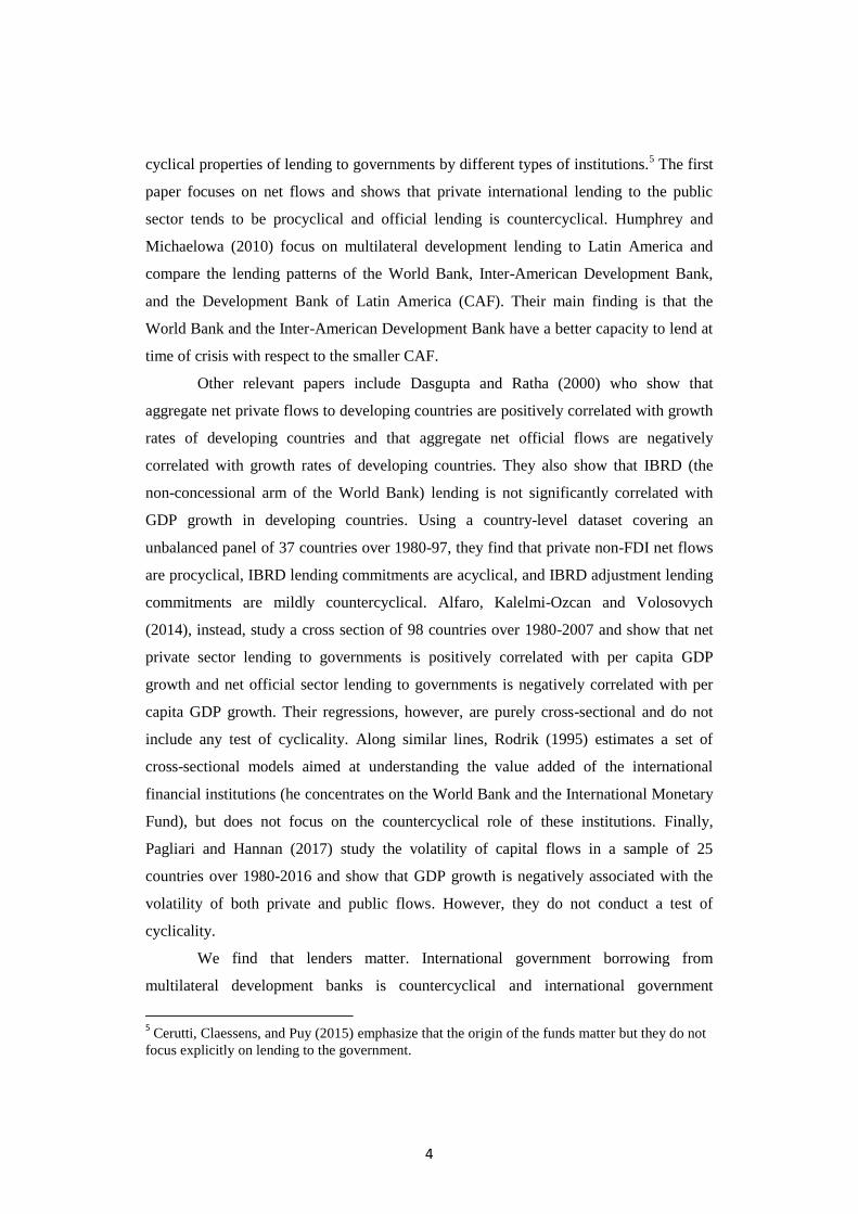
cyclical properties of lending to governments by different types of institutions.5 The first

paper focuses on net flows and shows that private international lending to the public

sector tends to be procyclical and official lending is countercyclical. Humphrey and

Michaelowa (2010) focus on multilateral development lending to Latin America and

compare the lending patterns of the World Bank, Inter-American Development Bank,

and the Development Bank of Latin America (CAF). Their main finding is that the

World Bank and the Inter-American Development Bank have a better capacity to lend at

time of crisis with respect to the smaller CAF.

Other relevant papers include Dasgupta and Ratha (2000) who show that

aggregate net private flows to developing countries are positively correlated with growth

rates of developing countries and that aggregate net official flows are negatively

correlated with growth rates of developing countries. They also show that IBRD (the

non-concessional arm of the World Bank) lending is not significantly correlated with

GDP growth in developing countries. Using a country-level dataset covering an

unbalanced panel of 37 countries over 1980-97, they find that private non-FDI net flows

are procyclical, IBRD lending commitments are acyclical, and IBRD adjustment lending

commitments are mildly countercyclical. Alfaro, Kalelmi-Ozcan and Volosovych

(2014), instead, study a cross section of 98 countries over 1980-2007 and show that net

private sector lending to governments is positively correlated with per capita GDP

growth and net official sector lending to governments is negatively correlated with per

capita GDP growth. Their regressions, however, are purely cross-sectional and do not

include any test of cyclicality. Along similar lines, Rodrik (1995) estimates a set of

cross-sectional models aimed at understanding the value added of the international

financial institutions (he concentrates on the World Bank and the International Monetary

Fund), but does not focus on the countercyclical role of these institutions. Finally,

Pagliari and Hannan (2017) study the volatility of capital flows in a sample of 25

countries over 1980-2016 and show that GDP growth is negatively associated with the

volatility of both private and public flows. However, they do not conduct a test of

cyclicality.

We find that lenders matter. International government borrowing from

multilateral development banks is countercyclical and international government

5 Cerutti, Claessens, and Puy (2015) emphasize that the origin of the funds matter but they do not

focus explicitly on lending to the government.

5

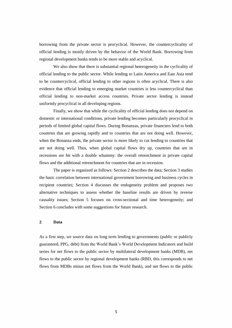
borrowing from the private sector is procyclical. However, the countercyclicality of

official lending is mostly driven by the behavior of the World Bank. Borrowing from

regional development banks tends to be more stable and acyclical.

We also show that there is substantial regional heterogeneity in the cyclicality of

official lending to the public sector. While lending to Latin America and East Asia tend

to be countercyclical, official lending to other regions is often acyclical. There is also

evidence that official lending to emerging market countries is less countercyclical than

official lending to non-market access countries. Private sector lending is instead

uniformly procyclical in all developing regions.

Finally, we show that while the cyclicality of official lending does not depend on

domestic or international conditions, private lending becomes particularly procyclical in

periods of limited global capital flows. During Bonanzas, private financiers lend to both

countries that are growing rapidly and to countries that are not doing well. However,

when the Bonanza ends, the private sector is more likely to cut lending to countries that

are not doing well. Thus, when global capital flows dry up, countries that are in

recessions are hit with a double whammy: the overall retrenchment in private capital

flows and the additional retrenchment for countries that are in recession.

The paper is organized as follows: Section 2 describes the data; Section 3 studies

the basic correlation between international government borrowing and business cycles in

recipient countries; Section 4 discusses the endogeneity problem and proposes two

alternative techniques to assess whether the baseline results are driven by reverse

causality issues; Section 5 focuses on cross-sectional and time heterogeneity; and

Section 6 concludes with some suggestions for future research.

2 Data

As a first step, we source data on long term lending to governments (public or publicly

guaranteed, PPG, debt) from the World Bank’s World Development Indicators and build

series for net flows to the public sector by multilateral development banks (MDB), net

flows to the public sector by regional development banks (RBD, this corresponds to net

flows from MDBs minus net flows from the World Bank), and net flows to the public

6

sector by private lenders.6 Net flows from MDBs and RDBs include both regular and

concessional lending and net flows from the private sector include both bonded debt and

international bank loans. We also build similar series for disbursements (i.e., new loans

not adjusted for repayments of existing loans and interest payments on existing loans).

As the World Development Indicators do not include debt data for countries that have

graduated to high-income status (for instance, the World Development Indicators do not

include debt data for Chile or South Korea), we recover these data by using old discs

from the World Bank’s Global Development Finance database (previously known as the

World Debt Tables).

We also use the World Development Indicators for data on GDP, which is then

used to compute different measures for each country’s output gap and to scale debt flows

(we use data in constant local currency units to compute the output gap and data in

current dollars to scale government debt). We use trade data from the World Integrated

Trade Solution (WITS) database to compute the external demand shock instrument

(more details on this below). Our final dataset is an unbalanced panel consisting of 3,804

observations covering up to 132 countries for the period 1980-2015 (pre-1980 data have

many missing observations).7

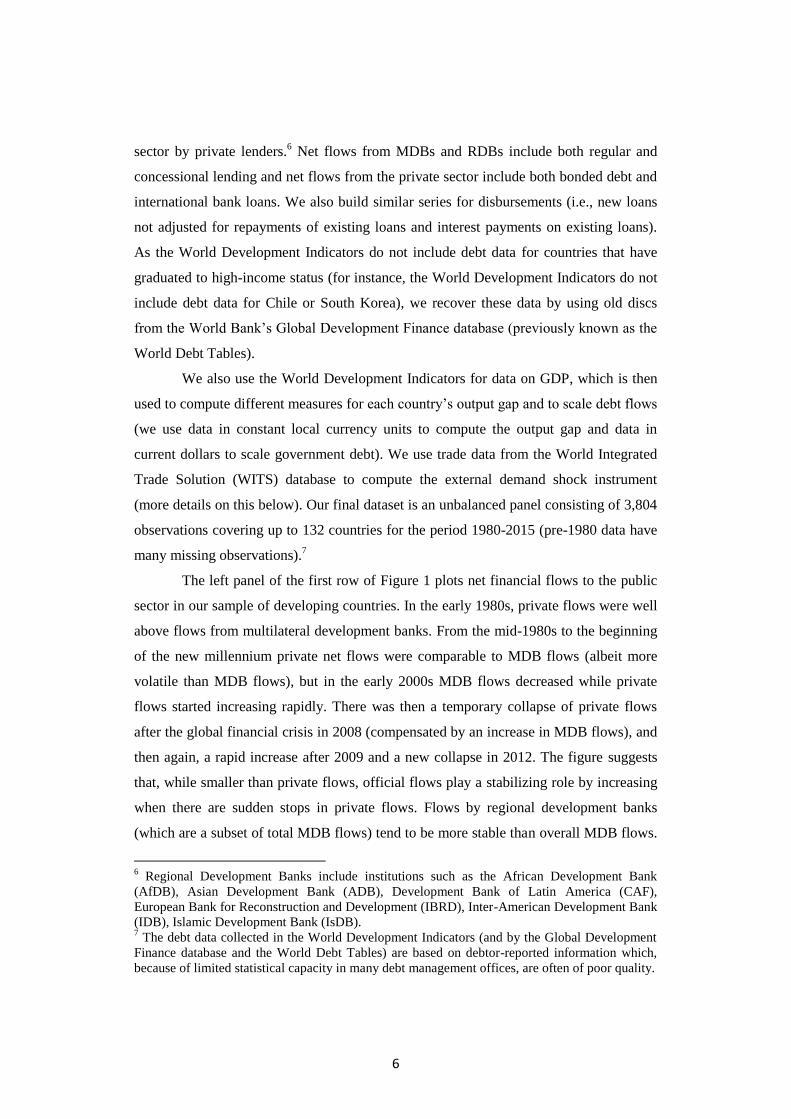
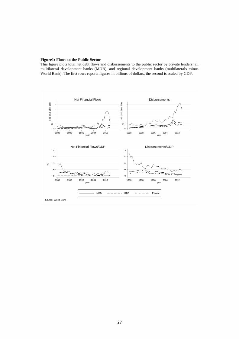
The left panel of the first row of Figure 1 plots net financial flows to the public

sector in our sample of developing countries. In the early 1980s, private flows were well

above flows from multilateral development banks. From the mid-1980s to the beginning

of the new millennium private net flows were comparable to MDB flows (albeit more

volatile than MDB flows), but in the early 2000s MDB flows decreased while private

flows started increasing rapidly. There was then a temporary collapse of private flows

after the global financial crisis in 2008 (compensated by an increase in MDB flows), and

then again, a rapid increase after 2009 and a new collapse in 2012. The figure suggests

that, while smaller than private flows, official flows play a stabilizing role by increasing

when there are sudden stops in private flows. Flows by regional development banks

(which are a subset of total MDB flows) tend to be more stable than overall MDB flows.

6 Regional Development Banks include institutions such as the African Development Bank

(AfDB), Asian Development Bank (ADB), Development Bank of Latin America (CAF),

European Bank for Reconstruction and Development (IBRD), Inter-American Development Bank

(IDB), Islamic Development Bank (IsDB). 7 The debt data collected in the World Development Indicators (and by the Global Development

Finance database and the World Debt Tables) are based on debtor-reported information which,

because of limited statistical capacity in many debt management offices, are often of poor quality.

7

The right panel of the first row of Figure 1 focuses on disbursements and shows patterns

which are similar to those of net flows.

The second row of Figure 1 reports the debt flows data scaled by the GDP of the

recipient country. The comparative pattern between private and MDB capital flows

described above can also be seen here. What is notable is the reduction in the size of

flows to governments with respect to GDP. This finding is the outcome of two related

phenomena. First, starting from the mid-1990s, several developing countries improved

their fiscal management and reduced their total government debt (even though debt

ratios increased in the aftermath of the global financial crisis, World Bank, 2017).

Second, after the financial crises of the 1990s, most developing countries decided that

foreign currency debt (and most external debt by developing countries is denominated in

foreign currency, Eichengreen, Hausmann, and Panizza, 2007) is too risky to be

sensible.8 Hence, they put in place policies aimed at developing domestic debt markets

which, for any given borrowing need, reduced the needs to issue international

government debt (Hausmann and Panizza, 2011).

3 Baseline Results

As a first step, we estimate a set of simple fixed effect models where we regress net

flows or disbursements to the public sector by different types of lenders over a country-

year specific output gap and a set of year and country fixed effects. Formally, we follow

Levy Yeyati (2008) and estimate the following model:

(1)

where is the flow of international government debt (measured as either net

flows or disbursement) over GDP by country in year , is the output gap in

country in year , and and are country and year fixed effects. We use three

measures of output gap: the percentage deviation between actual GDP and trend GDP

measured with the Hodrick-Prescott filter (this is our baseline), the percentage deviation

between actual GDP and trend GDP measured with a log-linear trend, and the Christiano

8 See also Dell’Erba, Hausmann, and Panizza (2013)

8

and Fitzgerald (2003) band pass filter. We also measure business cycle conditions by

simply looking at GDP growth.

In the set-up of Equation (1), a positive value of indicates that international

government borrowing is procyclical and a negative value of indicates that

international government borrowing is countercyclical. As Equation (1) includes year

fixed effects, it implicitly controls for all possible push factors (i.e., global shocks that

drive capital to developing countries).

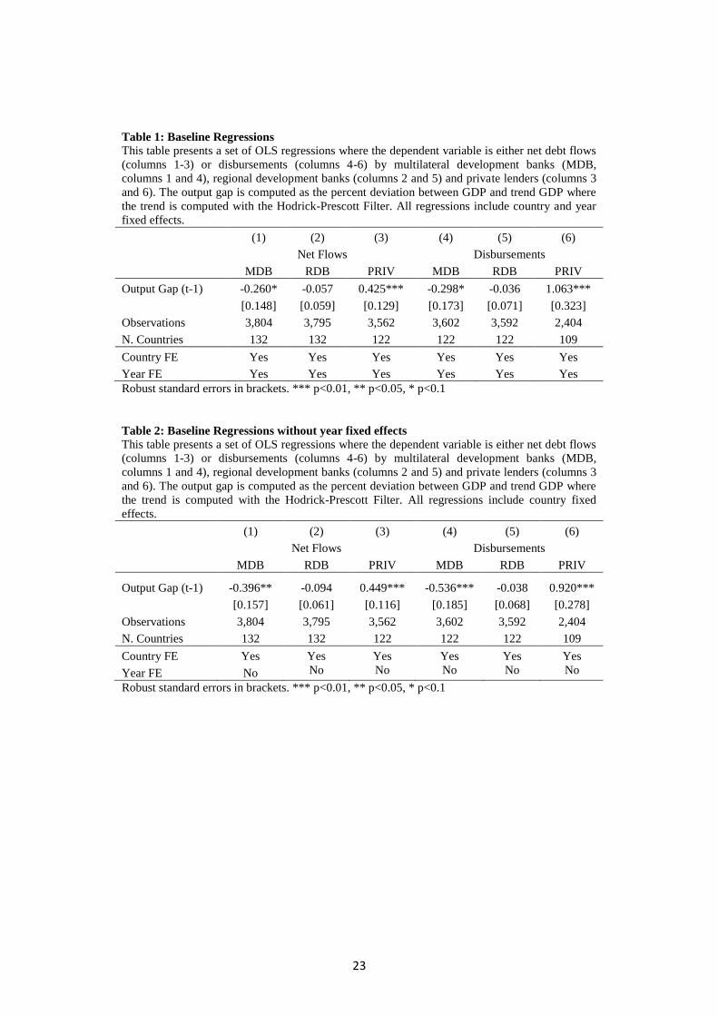
Table 1 reports the results of our baseline estimates where the output gap is

measured with the Hodrick-Prescott filter. When we focus on net flows by multilateral

development banks (MDB, column 1), we find a coefficient which is negative and

statistically significant. The point estimate suggests that when GDP is one standard

deviation below trend (0.28, see Table A1) net flows by multilateral development banks

increase by 0.07 percentage points of GDP. As the mean value of net flows by MDB is

1.18 percent of GDP, the point estimate implies that when the average country in our

sample is one standard deviation below trend GDP, net inflows by MDB increase by 6

percent with respect to their average value. When we focus on net flows by regional

development banks (RDB, column 2), we still find a negative coefficient (consistent with

countercyclicality), but in this case the point estimate is about one-fifth that for MDBs

and it is not statistically significant. The coefficient for private debt flows is instead

positive (consistent with procyclicality), quantitatively large, and statistically significant.

The point estimate implies that when GDP is one standard deviation below trend, private

flows decrease by approximately 0.12 percentage points, corresponding to one-third of

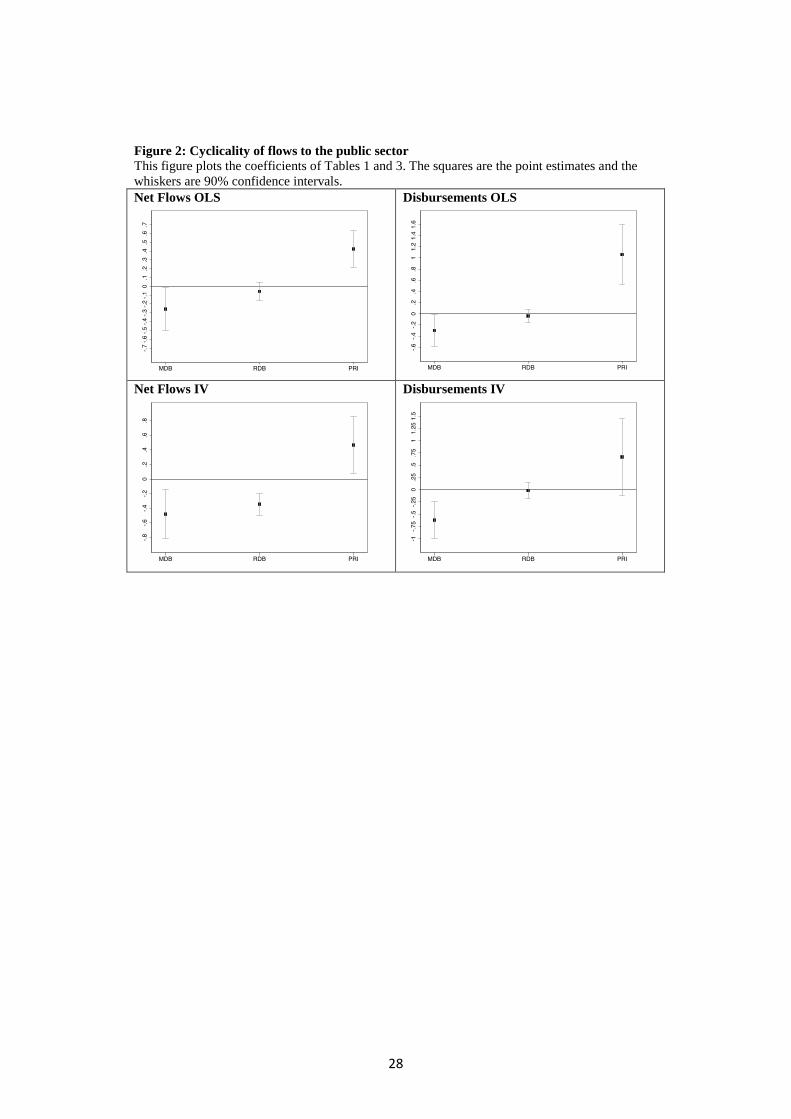
the cross-country average of 0.39 percent of GDP.9 The top left panel of Figure 2

presents a graphical illustration of the estimates of the first three columns of Table 1.

Columns 4-6 of Table 1 repeat the estimates of columns 1-3 by focusing on

disbursements instead of net flows. Again, we find evidence of countercyclicality for

disbursements by multilateral development banks and evidence of procyclicality for

disbursements by private lenders. Disbursements by regional development banks,

instead, are acyclical. The point estimates imply that when GDP is one standard

deviation below trend, disbursements by MDBs would increase by 4 percent with respect

9 0.425*0.28=0.119; 0.119/0.39=0.305.

9

to the average value of 1.9 percent of GDP and disbursements by private creditors would

decrease by 20 percent with respect to the average of 1.4 percent of GDP.

As noted above, the estimates of Table 1 include year fixed effects and

implicitly control for all global push factors that drive capital flows to developing

countries. If we re-run the regressions without controlling for year fixed effects, we find

that the coefficients for private flows are essentially identical to those of the regressions

that include year fixed effects (confront columns 3 and 6 of Table 1 with columns 3 and

6 of Table 2). The coefficients for regional development banks are somewhat larger (in

absolute value) than those of the fixed effect regressions, but they remain insignificant

from a statistical point of view. Instead we find that the coefficients for public sector

lending by MDBs are much larger (50 percent larger when we focus on net flows and 80

percent larger when we focus on disbursements) in the regressions that do not control for

year fixed effects. This finding suggests that multilateral development banks are more

countercyclical in the presence of global shocks.

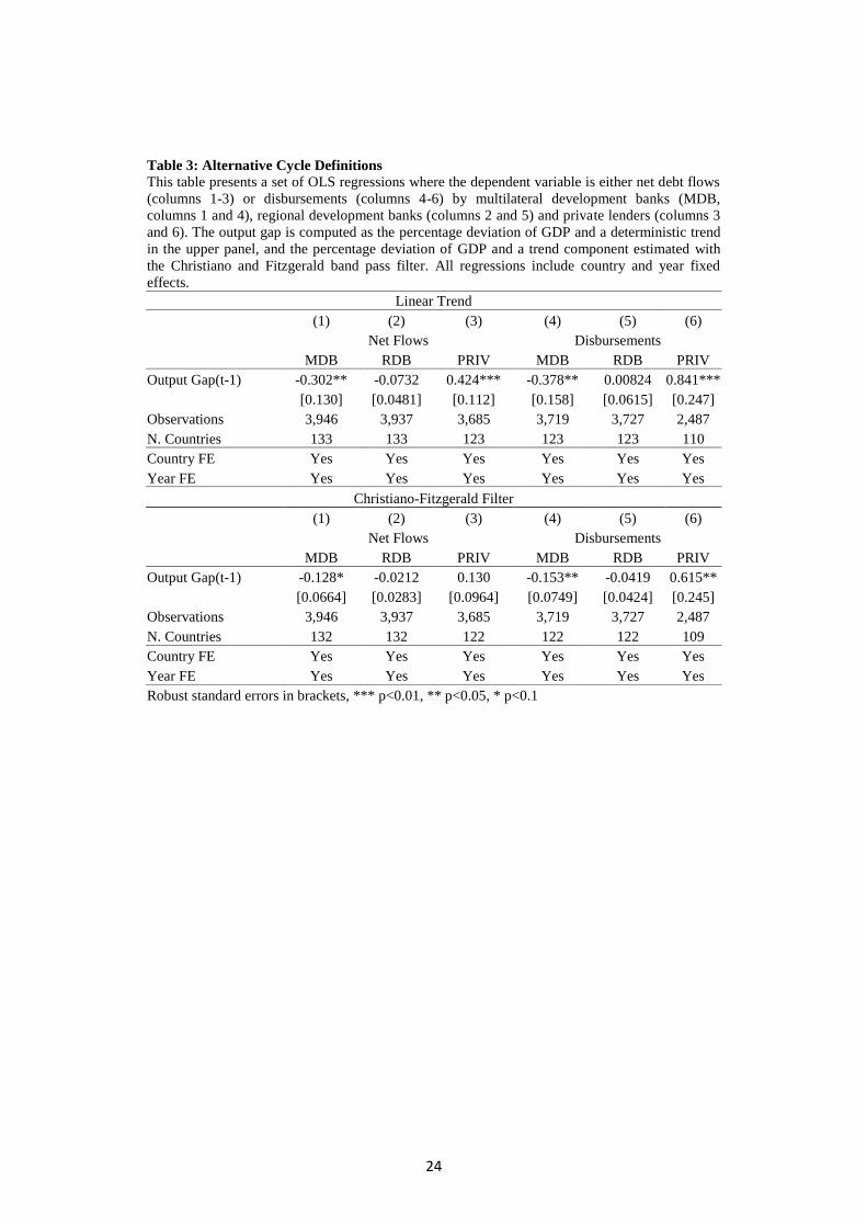
Table 3 reports results similar to those of Table 1, but with alternative measures

of the output gap. The upper panel of the table assumes that the long-term component of

output follows a linear trend. The cyclical component is the difference between the

logarithm of real output and a country-specific deterministic trend. The lower panel of

the table reports the same estimation using the Christiano and Fitzgerald band pass filter.

Both sets of results are in line with the estimations of Table 1. The evidence is robust

particularly in the disbursement equations where, regardless of the measure of the output

gap used, MDB lending is significantly countercyclical, RDB lending is acyclical, and

private lending is procyclical.

4 Endogeneity

Up to this point we assumed that in Equation (1) measures the causal effect of the

output gap on international government borrowing. This is equivalent to assuming that

the output gap is fully exogenous and hence uncorrelated with the residuals of Equation

(1) However, this assumption is unlikely to hold. Consider, for instance a model in

which the output gap (G) affects international government borrowing (D):

(2)

10

where and are parameters to be estimated and is a shock to international

government borrowing. In the setup of Equation (2), procyclicality would be associated

with a positive and a countercyclical fiscal policy with a negative . Note that

Equation (2) resembles Equation (1), and the interpretation of in Equation (2) is

exactly the interpretation that the traditional literature has given to the point estimates of

in Equation (1), i.e., the cyclicality of international government borrowing.

This interpretation would not be a problem if G were exogenous with respect to

expenditure. However, there is a large literature on the effect of capital inflows, or more

in general debt, which shows that inflows or debt have effects on growth. This

relationship can be described as:

(3)

where and are parameters to be estimated and is a shock to output. The parameter

k measures the effect of international debt on GDP and can take either a positive value

(capital inflows stimulate output) or a negative value (external debt is bad for growth).

The OLS estimation of from Equation (1) is:

(4)

and the bias of the OLS estimate is:

( ) ( )

⁄ (5)

Under the assumption that (this is a standard requirement for the convergence of

the system of Equations (2) and (3)), OLS estimates of are positively biased if

and negatively biased if

While the size of the bias depends on the direction of the bias only depends

on Hence, as long as the sign of the parameters of Equation (3) do not depend on the

type of lender, differences between the estimated degree of cyclicality of international

11

government borrowing from official and private lenders is not driven by the endogeneity

of the output gap.

Be as it may, we use two different strategies to address endogeneity concerns.

First, we instrument the output gap with an exogenous output gap built using a real

external shock consisting of the weighted average of GDP growth in country i’s export

partners. As a first step, we build the real external shock as:

∑ (6)

where GDPGRj,t measures real GDP growth in country j in period t, ij,t is the fraction of

exports from country i going to country j at time t, and EXPi/GDPi measures country's i

average exports expressed as a share of GDP. Note that we use a time-invariant measure

of exports over GDP. This is because a time-variant measure would be affected by real

exchange rate fluctuations, and, therefore, by domestic factors. This is not the case for

the fraction of exports going to a specific country (ij,t) because the variation of the

exchange rate that is due to domestic factors has an equal effect in both the numerator

and denominator. Next, we use GDPGRj,t to build an index for trading partners’ GDP

and use the Hodrick Prescott filter to compute the trend of this index. Finally, we build

an instrument for the output gap by computing the percentage deviation between actual

trading partners’ GDP and trend trading partners’ GDP.

A good instrument needs to be correlated with the instrumented variable (output

gap) and be exogenous with respect to the endogenous variable. The last row of Table 4

shows that the external shock measure is not a weak instrument. Exogeneity is assured

by the fact that exports to the countries that are influenced by the domestic country shock

tend to be a small fraction of the exports of the country that originated the shock.10

10

A detailed explanation is in Jaimovich and Panizza (2007). Based on their work and to

illustrate the idea, consider the case of Brazil and Uruguay. A shock to the Brazilian GDP will

have a large effect on the GDP of Uruguay and hence GDP growth in Uruguay will not be a good

instrument for GDP growth in Brazil, but Uruguay consists of a minuscule share of total exports

of Brazil (0.7 percent) and hence has almost no weight in Equation (6). Consider now Uruguay as

a source country. In this case, exports to Brazil have a large weight on total exports of Uruguay

(16 percent) but a shock to Uruguay’s GDP will have basically no effect on Brazil’s GDP and

this, again, should reduce concerns of reverse causality. The same reasoning applies to pairs of

medium size countries. Consider for instance the case of Italy and France (which are each other’s

main trading partner, we abstract from the fact that these countries are not in our sample) and

focus on how a shock that originates in Italy affects France and then feeds back to Italy. France

12

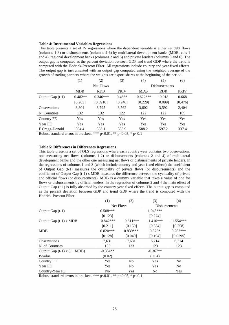
The IV regressions corroborate our previous result that official lending to the

public sector is countercyclical and private sector lending procyclical. Regressions that

focus on net debt flows find negative and statistically significant coefficients for both

MDB and RDB net flows (the RDB coefficient is negative and not statistically

significant in the OLS regressions of Table 1) and positive and statistically significant

for net flows by private lenders (columns 1-3 of Table 4). While the instrumental

variables coefficients for the MDB and RDB regressions are much larger than the OLS

coefficients (85 percent larger for the MDB coefficient and 6 times larger for the RDB

coefficient), the IV coefficient for private sector lending is essentially identical to the

OLS coefficients. The last three columns of Table 3 focus on disbursements. Also in this

case, the coefficient for MDB lending is larger than the OLS coefficient (about twice as

large), but the RDB coefficient in the IV estimates is similar to the OLS one. The private

sector coefficient is 40 percent lower than the OLS coefficient and not statistically

significant (however, with a p-value of 14 is not too far from being statistically

significant at the 10 percent confidence level).

Taken together, the IV regressions suggest that the countercyclicality of MDB

lending and the procyclicality of net flows by private sector lenders are not driven by

reverse causality. In fact, OLS regressions may underestimate the degree of

countercyclicality of official lending (both MDB and RDB). While the IV regressions

indicate that OLS estimations may overstate the degree of procyclicality of private sector

disbursements, correcting for potential endogeneity does not alter the results that MDB

flows are countercyclical and private flows are procyclical.

Our second strategy consists of pooling together net flows and disbursements by

private and official lenders so that our dataset consists of two observations for each

country-year. We start by estimating the following model:

( ) (7)

exports-to-GDP ratio is about 25 percent and France share of exports to Italy is 9 percent.

Jaimovich and Panizza (2007) estimate that a 1 percent shock to Italy’s GDP growth translates

into a 0.25*0.09*2=0.045 percent shock to French GDP. Now consider the feedback to Italy of

this shock (which would be the source of reverse causality). Italy’s export-to-GDP ratio is also

around 25 percent and Italy’s share of exports to France is 12 percent. Hence, we obtain:

0.045*0.25*0.12*2=0.002, this is greater than zero but a minuscule fraction (one fifth of a

percentage point) of the original shock.

13

where is international government borrowing by country , in year from

borrower type (where is either MDB or private sector lenders) and is a dummy

variable that takes value one for MDB lending. In this set-up, measures the cyclicality

of private lending, is the difference between the cyclicality of private sector and MDB

lending, and is the cyclicality of MDB lending. Column 1 of Table 5 confirms that

private lending is procyclical, official lending is countercyclical, and the difference

between the cyclicality of private and official lending is statistically significant. Equation

(7) does not solve the endogeneity problem because could still be correlated

with . However, we can estimate the following difference-in-difference specification:

( ) (8)

where are country-year fixed effects. While model (8) only allows estimating the

difference between the cyclicality of private and MDB lending, it does not suffer from

any obvious endogeneity problem, because the potential correlation between the output

gap and the error term is fully captured by the country-year fixed effects. Column 2 of

Table 5 shows that the coefficient in Equation (8) is almost identical to that of

Equation (7). This finding is consistent with the assumption that the estimates of

Equation (7) are unbiased. Columns 3 and 4 estimate Equations (7) and (8) using

disbursements instead of net flows and find results which are essentially identical to

those of columns 1 and 2.

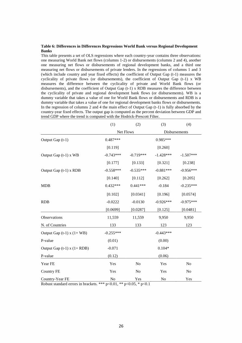
In Table 6, we estimate a model similar to that of Equations (7) and (8) but split

lending by MDBs into World Bank lending and RDB lending. We find that private net

flows and disbursements are procyclical, World Bank flows and disbursements are

countercyclical, and RDB flows and disbursement are either acyclical or mildly

procyclical (column 3) but significantly less procyclical than private flows. As before,

we find that the differences-in-differences estimates of columns 2 and 4 are similar to

those of columns 1 and 3.

Taken together these results corroborate theoretical arguments, suggesting that

controlling for endogeneity does not affect our baseline results that MDB flows and

disbursements are countercyclical, RDB flows and disbursements acyclical, and private

flows and disbursements procyclical. Since IV estimations are less efficient than OLS

14

estimations, from here on we focus on OLS estimations (in most cases, the IV results are

similar to the OLS results).

5 Heterogeneity

We explore two types of heterogeneity: cross sectional and over time. When we look at

cross-sectional heterogeneity, we study whether the cyclical properties of international

government borrowing vary across developing regions and we also check whether there

are differences between emerging market and low income countries. When we focus on

over time heterogeneity, we study whether cyclicality remains the same throughout time,

or if it varies with the business cycle.11

5.1 Cross-sectional heterogeneity

We start by exploring cross-sectional heterogeneity by splitting our sample into separate

developing regions. Specifically, we use the World Bank Classification and partition our

132 countries into 6 regions: East Asia and the Pacific (EAP, 12 countries), East Europe

and Central Asia (ECA, 28 countries), Latin American and the Caribbean (LAC, 26

countries), Middle East and North Africa (MNA, 11 countries), South Asia (SAS, 7

countries), and Sub-Saharan Africa (SSA 41 countries).

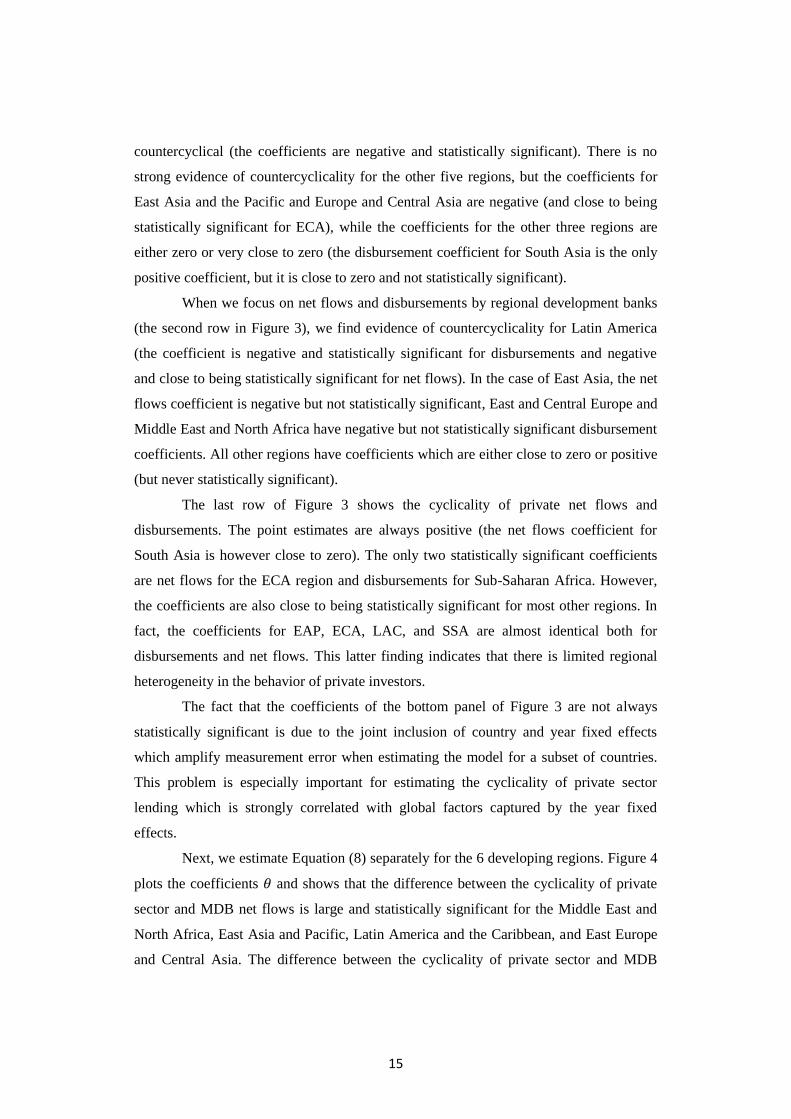
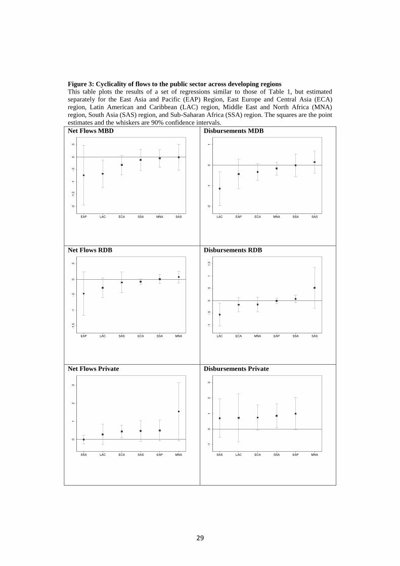
Figure 3 reports the estimates of Equation (1) for the six regions. The figures in

the first column focus on net flows and the figures in the second column on

disbursements. In each panel, regions are ordered from the most countercyclical (or least

procyclical) to the most procyclical (or least countercyclical). The top two panels show

that MDB flows and disbursements to Latin America and the Caribbean are

11

There are several reasons that could suggest changes over time in the response of MDBs to

fluctuations in the business cycle of their clients. For example, lenders can be countercyclical in

bad times but not in good times, or cyclicality can change for reasons that are different from the

business cycle itself. Consider for example changes in how MDBs incorporate country risk in

their capital adequacy requirements. Different capital adequacy models can lead to different

responses to economic cycles. If a country is downgraded during a recession, and the downgrade

increases capital requirements for MDBs, then the MDB may respond procyclically by reducing

its exposure to the downgraded country. On the other hand, if the financial strength of the

multilateral is not affected by a downgrade of its clients and it does not need to increase capital

requirements, then the MDB can respond countercyclically to the demands of the downgraded

country.

15

countercyclical (the coefficients are negative and statistically significant). There is no

strong evidence of countercyclicality for the other five regions, but the coefficients for

East Asia and the Pacific and Europe and Central Asia are negative (and close to being

statistically significant for ECA), while the coefficients for the other three regions are

either zero or very close to zero (the disbursement coefficient for South Asia is the only

positive coefficient, but it is close to zero and not statistically significant).

When we focus on net flows and disbursements by regional development banks

(the second row in Figure 3), we find evidence of countercyclicality for Latin America

(the coefficient is negative and statistically significant for disbursements and negative

and close to being statistically significant for net flows). In the case of East Asia, the net

flows coefficient is negative but not statistically significant, East and Central Europe and

Middle East and North Africa have negative but not statistically significant disbursement

coefficients. All other regions have coefficients which are either close to zero or positive

(but never statistically significant).

The last row of Figure 3 shows the cyclicality of private net flows and

disbursements. The point estimates are always positive (the net flows coefficient for

South Asia is however close to zero). The only two statistically significant coefficients

are net flows for the ECA region and disbursements for Sub-Saharan Africa. However,

the coefficients are also close to being statistically significant for most other regions. In

fact, the coefficients for EAP, ECA, LAC, and SSA are almost identical both for

disbursements and net flows. This latter finding indicates that there is limited regional

heterogeneity in the behavior of private investors.

The fact that the coefficients of the bottom panel of Figure 3 are not always

statistically significant is due to the joint inclusion of country and year fixed effects

which amplify measurement error when estimating the model for a subset of countries.

This problem is especially important for estimating the cyclicality of private sector

lending which is strongly correlated with global factors captured by the year fixed

effects.

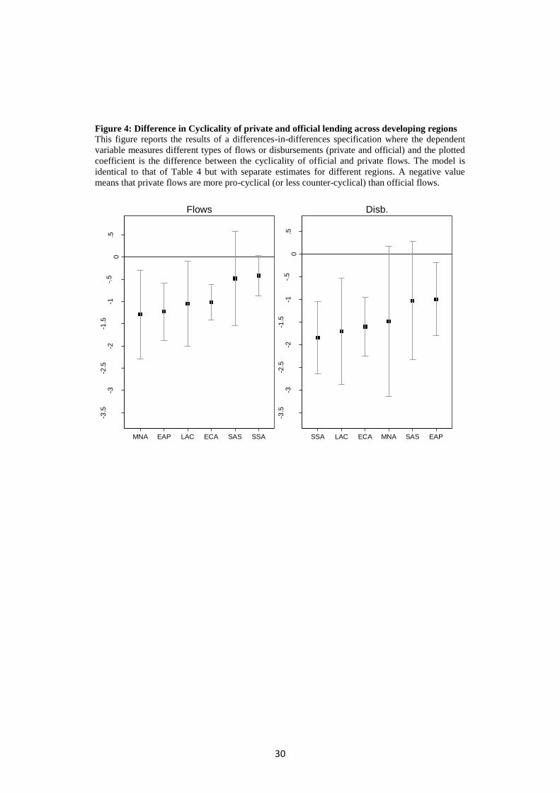
Next, we estimate Equation (8) separately for the 6 developing regions. Figure 4

plots the coefficients and shows that the difference between the cyclicality of private

sector and MDB net flows is large and statistically significant for the Middle East and

North Africa, East Asia and Pacific, Latin America and the Caribbean, and East Europe

and Central Asia. The difference between the cyclicality of private sector and MDB

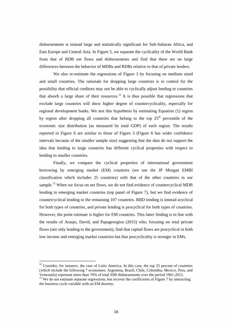
16

disbursements is instead large and statistically significant for Sub-Saharan Africa, and

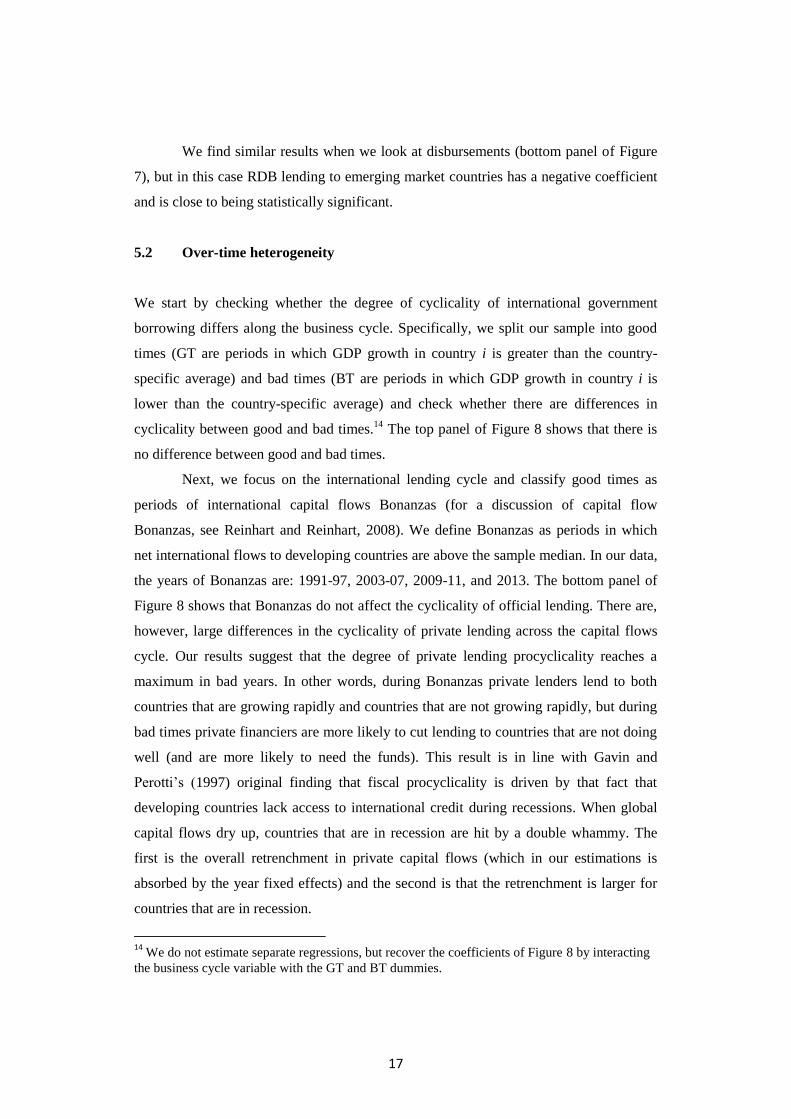
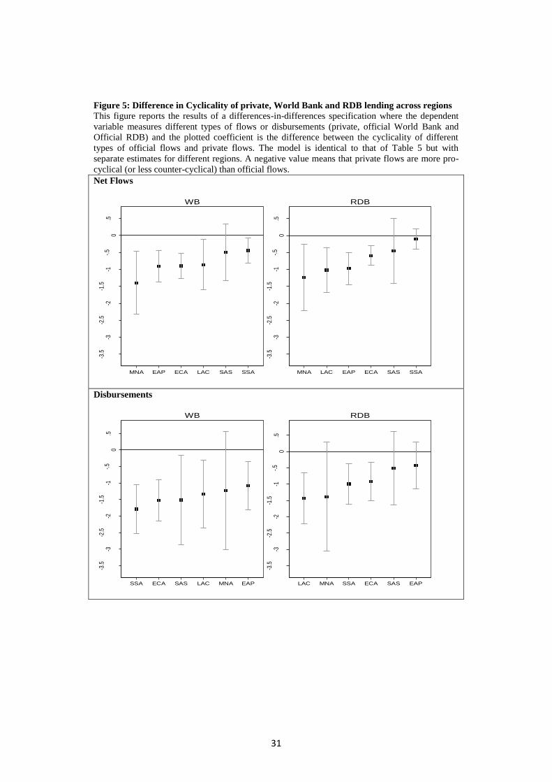
East Europe and Central Asia. In Figure 5, we separate the cyclicality of the World Bank

from that of RDB net flows and disbursements and find that there are no large

differences between the behavior of MDBs and RDBs relative to that of private lenders.

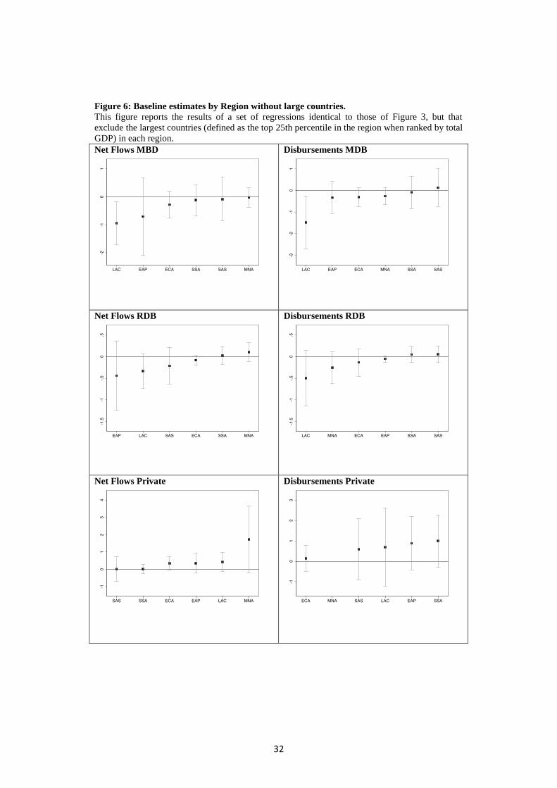
We also re-estimate the regressions of Figure 3 by focusing on medium sized

and small countries. The rationale for dropping large countries is to control for the

possibility that official creditors may not be able to cyclically adjust lending to countries

that absorb a large share of their resources.12

It is thus possible that regressions that

exclude large countries will show higher degree of countercyclicality, especially for

regional development banks. We test this hypothesis by estimating Equation (1) region

by region after dropping all countries that belong to the top 25th percentile of the

economic size distribution (as measured by total GDP) of each region. The results

reported in Figure 6 are similar to those of Figure 3 (Figure 6 has wider confidence

intervals because of the smaller sample size) suggesting that the data do not support the

idea that lending to large countries has different cyclical properties with respect to

lending to smaller countries.

Finally, we compare the cyclical properties of international government

borrowing by emerging market (EM) countries (we use the JP Morgan EMBI

classification which includes 25 countries) with that of the other countries in our

sample.13

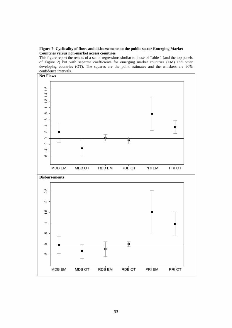
When we focus on net flows, we do not find evidence of countercyclical MDB

lending to emerging market countries (top panel of Figure 7), but we find evidence of

countercyclical lending to the remaining 107 countries. RBD lending is instead acyclical

for both types of countries, and private lending is procyclical for both types of countries.

However, the point estimate is higher for EM countries. This latter finding is in line with

the results of Araujo, David, and Papageorgiou (2015) who, focusing on total private

flows (not only lending to the government), find that capital flows are procyclical in both

low income and emerging market countries but that procyclicality is stronger in EMs.

12

Consider, for instance, the case of Latin America. In this case, the top 25 percent of countries

(which include the following 7 economies: Argentina, Brazil, Chile, Colombia, Mexico, Peru, and

Venezuela) represent more than 70% of total IDB disbursements over the period 1961-2015. 13

We do not estimate separate regressions, but recover the coefficients of Figure 7 by interacting

the business cycle variable with an EM dummy.

17

We find similar results when we look at disbursements (bottom panel of Figure

7), but in this case RDB lending to emerging market countries has a negative coefficient

and is close to being statistically significant.

5.2 Over-time heterogeneity

We start by checking whether the degree of cyclicality of international government

borrowing differs along the business cycle. Specifically, we split our sample into good

times (GT are periods in which GDP growth in country i is greater than the country-

specific average) and bad times (BT are periods in which GDP growth in country i is

lower than the country-specific average) and check whether there are differences in

cyclicality between good and bad times.14

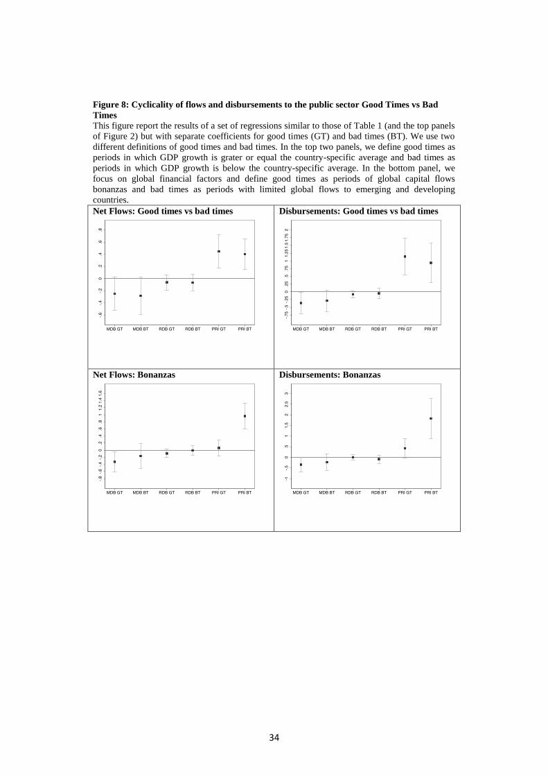
The top panel of Figure 8 shows that there is

no difference between good and bad times.

Next, we focus on the international lending cycle and classify good times as

periods of international capital flows Bonanzas (for a discussion of capital flow

Bonanzas, see Reinhart and Reinhart, 2008). We define Bonanzas as periods in which

net international flows to developing countries are above the sample median. In our data,

the years of Bonanzas are: 1991-97, 2003-07, 2009-11, and 2013. The bottom panel of

Figure 8 shows that Bonanzas do not affect the cyclicality of official lending. There are,

however, large differences in the cyclicality of private lending across the capital flows

cycle. Our results suggest that the degree of private lending procyclicality reaches a

maximum in bad years. In other words, during Bonanzas private lenders lend to both

countries that are growing rapidly and countries that are not growing rapidly, but during

bad times private financiers are more likely to cut lending to countries that are not doing

well (and are more likely to need the funds). This result is in line with Gavin and

Perotti’s (1997) original finding that fiscal procyclicality is driven by that fact that

developing countries lack access to international credit during recessions. When global

capital flows dry up, countries that are in recession are hit by a double whammy. The

first is the overall retrenchment in private capital flows (which in our estimations is

absorbed by the year fixed effects) and the second is that the retrenchment is larger for

countries that are in recession.

14

We do not estimate separate regressions, but recover the coefficients of Figure 8 by interacting

the business cycle variable with the GT and BT dummies.

18

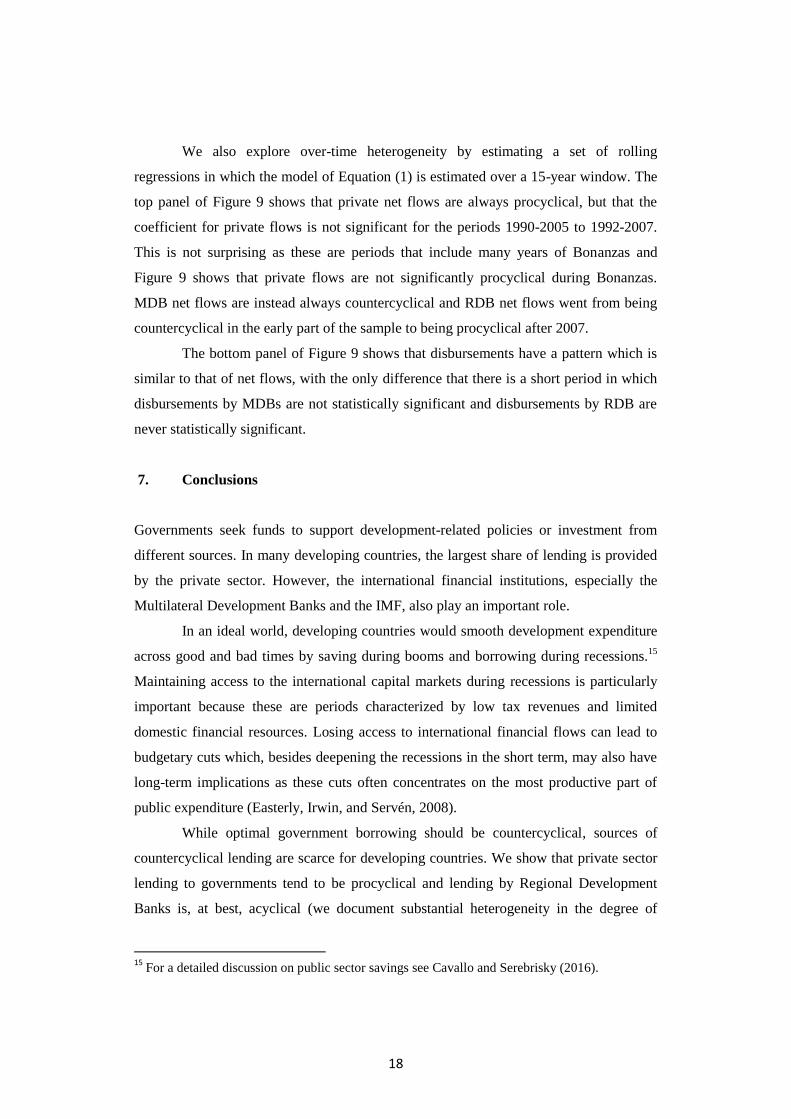
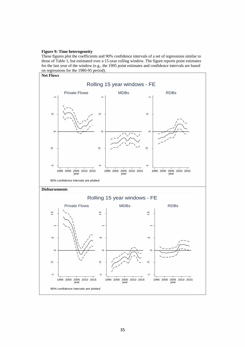
We also explore over-time heterogeneity by estimating a set of rolling

regressions in which the model of Equation (1) is estimated over a 15-year window. The

top panel of Figure 9 shows that private net flows are always procyclical, but that the

coefficient for private flows is not significant for the periods 1990-2005 to 1992-2007.

This is not surprising as these are periods that include many years of Bonanzas and

Figure 9 shows that private flows are not significantly procyclical during Bonanzas.

MDB net flows are instead always countercyclical and RDB net flows went from being

countercyclical in the early part of the sample to being procyclical after 2007.

The bottom panel of Figure 9 shows that disbursements have a pattern which is

similar to that of net flows, with the only difference that there is a short period in which

disbursements by MDBs are not statistically significant and disbursements by RDB are

never statistically significant.

7. Conclusions

Governments seek funds to support development-related policies or investment from

different sources. In many developing countries, the largest share of lending is provided

by the private sector. However, the international financial institutions, especially the

Multilateral Development Banks and the IMF, also play an important role.

In an ideal world, developing countries would smooth development expenditure

across good and bad times by saving during booms and borrowing during recessions.15

Maintaining access to the international capital markets during recessions is particularly

important because these are periods characterized by low tax revenues and limited

domestic financial resources. Losing access to international financial flows can lead to

budgetary cuts which, besides deepening the recessions in the short term, may also have

long-term implications as these cuts often concentrates on the most productive part of

public expenditure (Easterly, Irwin, and Servén, 2008).

While optimal government borrowing should be countercyclical, sources of

countercyclical lending are scarce for developing countries. We show that private sector

lending to governments tend to be procyclical and lending by Regional Development

Banks is, at best, acyclical (we document substantial heterogeneity in the degree of

15

For a detailed discussion on public sector savings see Cavallo and Serebrisky (2016).

19

cyclicality of RDB lending). Only the World Bank lends against the business cycle, and

this is not even the case in all developing regions.

Besides documenting differences across types of lenders, we also show that there

has been a change in the cyclicality of lending by Regional Development Banks. These

institutions went from being countercyclical in the 1990s to being procyclical in the

aftermath of the global financial crisis. Why did this happen?

One possibility is that procyclicality is driven by the fact that many RDBs have

no flexibility to lend more in bad times because they have reached their lending capacity.

By itself, this explanation would be consistent with acyclicality (rather than

procyclicality). However, a lending limit could lead to procyclicality if the limit becomes

tighter in bad times. A reason why the limit could become tighter in bad times is related

to recent changes in the way in which rating agencies assess the risk of Multilateral

Development Banks and to the greater weight these agencies give to the rating of the

countries that borrow from the MDBs (see Humphrey, 2016, for details). Consider, for

instance, a situation in which a large borrower (or many small borrowers) of an MDB

goes into recession and is downgraded by the main rating agencies with potential effects

on the rating of the MDB. Then, the MDB can either accept the risk of a downgrade, or

seek a capital increase, or increase its capital ratio by reducing lending. As the first

option can have large economic and political cost and the second option requires a multi-

year process of consensus building among the MDB’s shareholders, the most likely

outcome is a reduction in lending. Such reduction in lending will lead to the procyclical

behavior which we observe in the data. Such an outcome is more likely to be observed in

the less diversified RDBs than in an institution like the World Bank which has global

coverage.

In future research, it would be interesting to test whether changes in the degree

of cyclicality of RDB lending are indeed driven by the interaction between changes in

the rating methodology and the possibility that most RDBs have reached their lending

limit.

20

References

Alesina, Alberto, Filipe R. Campante, and Guido Tabellini, 2008. "Why is Fiscal Policy

Often Procyclical?," Journal of the European Economic Association, vol. 6(5), pages

1006-1036, 09

Alfaro, Laura, Sebnem Kalemli-Ozcan, and Vadym Volosovych, 2014. "Sovereigns,

Upstream Capital Flows and Global Imbalances." Journal of the European Economic

Association

Araujo, Juliana, Antonio David, and Chris Papageorgiou, 2015. “Joining the Club?

Procyclicality of Private Capital Flows in Low Income Developing Countries,” IMF

Working Paper N. 15/163.

Barro, Robert, 1979. “On the determination of the public debt.” Journal of Political

Economy 87(5): 940-971

Calvo, Guillermo, Leonardo Leiderman, and Carmen Reinhart, 1993. “Capital Flows and

Real Exchange Rate in Appreciation on Latin America: The Role of External Factors,”

IMF Staff Papers, 40(1): 108-151.

Cavallo, Eduardo and Tomás Serebrisky, 2016. Saving for Development; How Latin

America and the Caribbean can Save More and Better, Washington DC: Palgrave.

Cerutti, Eugenio, Stijn Claessens, and Damien Puy, 2015. “ Push Factors and capital

Flows to Emerging Markets: Why Knowing Your Lender Matters More Than

Fundamentals,” IMF Working Paper 15/127.

Christiano, Lawrence and Terry Fitzgerald, 2003. “The band pass filter.” International

Economic Review 44: 435-465.

Dasgupta, Dipak and Dilip Ratha, 2000. “What factors appear to drive private capital

flows to developing countries? and how does official lending respond?” World Bank

Policy Research Working Paper WPS 2392

Dell’Erba, Salvatore, Ricardo Hausmann, and Ugo Panizza, 2013. "Debt levels, debt

composition, and sovereign spreads in emerging and advanced economies," Oxford

Review of Economic Policy, 29: 518-547.

Easterly, William, Timothy Irwin, and Luis Servén, 2008. "Walking up the Down

Escalator: Public Investment and Fiscal Stability," World Bank Research Observer, vol.

23(1): pages 37-56.

Eichengreen, Barry, Ricardo Hausmann, and Ugo Panizza, 2007., “Currency

Mismatches, Debt Intolerance, and the Original Sin: Why They Are Not the Same and

Why It Matters,” in Capital Controls and Capital Flows in Emerging Economies:

21

Policies, Practices and Consequences, S. Edwards (ed.), National Bureau of Economic

Research, Inc. and Chicago University Press, Chicago.

Fernandez-Arias, Eduardo, 1996. “The new wave of private capital inflows: Push or

pull?” Journal of Development Economics, 48: 389-418.

Forbes, Kristin and Francis Warnock, 2012. "Capital flow waves: Surges, stops, flight,

and retrenchment," Journal of International Economics, 88(2): 235-251

Fratzscher, Marcel, 2012. "Capital flows, push versus pull factors and the global

financial crisis," Journal of International Economics, 88(2): 341-356.

Gavin, Michael and Roberto Perotti, 1997. “Fiscal Policy in Latin America,” in

Bernanke and Rotemberg (eds.) NBER Macroeconomics Annual 1997, Volume 12: 11-

72.

Hausmann, Ricardo and Ugo Panizza, 2011. “Redemption or Abstinence? Original Sin,

Currency Mismatches and Counter Cyclical Policies in the New Millennium,” Journal of

Globalization and Development, 2(1)

Humphrey Chris and Katharina Michaelowa, 2010. “The Business of Development:

Trends in Lending by Multilateral Development Banks to Latin America, 1980‐2009,”

mimeo, University of Zurich.

Humphrey, Chris, 2016. “The Principal in the Shadows: Credit Rating Agencies and

Multilateral Development Banks”, mimeo University of Zurich.

Jaimovich, Dany and Ugo Panizza, 2007. "Procyclicality or Reverse Causality?,”

Research Department Publications 4508, Inter-American Development Bank, Research

Department.

Kaminsky, Graciela, Carmen Reinhart, and Carlos Végh, 2005. “When It Rains, It Pours:

Procyclical Capital Flows and Macroeconomic Policies,” in Gertler and Rogoff (eds.)

NBER Macroeconomics Annual 2004, Volume 19.

Levy Yeyati, Eduardo 2009. "Optimal Debt? On the Insurance Value of International

Debt Flows to Developing Countries," Open Economies Review, 20(4): 489-507.

Pagliari, Maria Sole and Swarnali Ahmed Hannan, 2017. “The Volatility of Capital

Flows in Emerging Markets: Measures and Determinants,” IMF WP 17/41

Reinhart, Carmen and Vincent Reinhart, 2008. “Capital Flow Bonanzas: An

Encompassing View of the Past and Present, NBER Working Paper No. 14321.

Rochet, Jean-Charles, 2006. “Optimal Sovereign Debt: An Analytical Approach.” Inter-

American Development Bank Research Department Working Paper 573.

22

Rodrik, Dani, 1995. “Why Is There Multilateral Lending?” Annual World Bank

Conference on Development Economics 1995: 167-193.

Talvi, Ernesto, and Carlos Vegh, 2005. “Tax Base Variability and Procyclical Fiscal

Policy in Developing Countries.” Journal of Development Economics, 78(1): 156–90.

Tornell, Aaron, and Philip Lane, 1999. “The Voracity Effect.” American Economic

Review, 89(1): 22–46.

World Bank, 2017. Global Economic Prospects, June

23

Table 1: Baseline Regressions

This table presents a set of OLS regressions where the dependent variable is either net debt flows

(columns 1-3) or disbursements (columns 4-6) by multilateral development banks (MDB,

columns 1 and 4), regional development banks (columns 2 and 5) and private lenders (columns 3

and 6). The output gap is computed as the percent deviation between GDP and trend GDP where

the trend is computed with the Hodrick-Prescott Filter. All regressions include country and year

fixed effects.

(1) (2) (3) (4) (5) (6)

Net Flows Disbursements

MDB RDB PRIV MDB RDB PRIV

Output Gap (t-1) -0.260* -0.057 0.425*** -0.298* -0.036 1.063***

[0.148] [0.059] [0.129] [0.173] [0.071] [0.323]

Observations 3,804 3,795 3,562 3,602 3,592 2,404

N. Countries 132 132 122 122 122 109

Country FE Yes Yes Yes Yes Yes Yes

Year FE Yes Yes Yes Yes Yes Yes

Robust standard errors in brackets. *** p<0.01, ** p<0.05, * p<0.1

Table 2: Baseline Regressions without year fixed effects




and 6). The output gap is computed as the percent deviation between GDP and trend GDP where

the trend is computed with the Hodrick-Prescott Filter. All regressions include country fixed

effects.

(1) (2) (3) (4) (5) (6)



Output Gap (t-1) -0.396** -0.094 0.449*** -0.536*** -0.038 0.920***

[0.157] [0.061] [0.116] [0.185] [0.068] [0.278]

Observations 3,804 3,795 3,562 3,602 3,592 2,404

N. Countries 132 132 122 122 122 109


Year FE No No No No No No


24

Table 3: Alternative Cycle Definitions




and 6). The output gap is computed as the percentage deviation of GDP and a deterministic trend

in the upper panel, and the percentage deviation of GDP and a trend component estimated with

the Christiano and Fitzgerald band pass filter. All regressions include country and year fixed

effects.

Linear Trend

(1) (2) (3) (4) (5) (6)



Output Gap(t-1) -0.302** -0.0732 0.424*** -0.378** 0.00824 0.841***

[0.130] [0.0481] [0.112] [0.158] [0.0615] [0.247]

Observations 3,946 3,937 3,685 3,719 3,727 2,487

N. Countries 133 133 123 123 123 110



Christiano-Fitzgerald Filter

(1) (2) (3) (4) (5) (6)



Output Gap(t-1) -0.128* -0.0212 0.130 -0.153** -0.0419 0.615**

[0.0664] [0.0283] [0.0964] [0.0749] [0.0424] [0.245]

Observations 3,946 3,937 3,685 3,719 3,727 2,487

N. Countries 132 132 122 122 122 109



Robust standard errors in brackets, *** p<0.01, ** p<0.05, * p<0.1

25

Table 4: Instrumental Variables Regressions

This table presents a set of IV regressions where the dependent variable is either net debt flows

(columns 1-3) or disbursements (columns 4-6) by multilateral development banks (MDB, cols 1

and 4), regional development banks (columns 2 and 5) and private lenders (columns 3 and 6). The

output gap is computed as the percent deviation between GDP and trend GDP where the trend is

computed with the Hodrick-Prescott Filter. All regressions include country and year fixed effects.

The output gap is instrumented with an output gap computed using the weighted average of the

growth of trading partners where the weights are export shares at the beginning of the period.

(1) (2) (3) (4) (5) (6)



Output Gap (t-1) -0.482** -0.346*** 0.466* -0.622*** -0.018 0.668

[0.203] [0.0910] [0.240] [0.229] [0.099] [0.476]

Observations 3,804 3,795 3,562 3,602 3,592 2,404

N. Countries 132 132 122 122 122 109



F Cragg-Donald 564.4 563.1 583.9 588.2 597.2 337.4


Table 5: Differences in Differences Regressions

This table presents a set of OLS regressions where each country-year contains two observations:

one measuring net flows (columns 1-2) or disbursements (columns 2 and 4) of multilateral

development banks and the other one measuring net flows or disbursements of private lenders. In

the regressions of columns 1 and 3 (which include country and year fixed effects) the coefficient

of Output Gap (t-1) measures the cyclicality of private flows (or disbursements) and the

coefficient of Output Gap (t-1) x MDB measures the difference between the cyclicality of private

and official flows (or disbursements). MDB is a dummy variable that takes a value of one for

flows or disbursements by official lenders. In the regression of columns 2 and 4 the main effect of

Output Gap (t-1) is fully absorbed by the country-year fixed effects. The output gap is computed

as the percent deviation between GDP and trend GDP where the trend is computed with the

Hodrick-Prescott Filter.

(1) (2) (3) (4)


Output Gap (t-1) 0.508***

1.043***

[0.123]

[0.274]

Output Gap (t-1) x MDB -0.842*** -0.811*** -1.410*** -1.554***

[0.211] [0.159] [0.334] [0.258]

MDB 0.820*** 0.839*** 0.375* 0.262***

[0.128] [0.040] [0.194] [0.0595]

Observations 7,631 7,631 6,214 6,214

N. of Countries 133 133 123 123

Output Gap (t-1) x (1+ MDB) -0.334**

-0.367**

P-value (0.02)

(0.04)

Country FE Yes No Yes No

Year FE Yes No Yes No

Country-Year FE No Yes No Yes


26

Table 6: Differences in Differences Regressions World Bank versus Regional Development

Banks

This table presents a set of OLS regressions where each country-year contains three observations:

one measuring World Bank net flows (columns 1-2) or disbursements (columns 2 and 4), another

one measuring net flows or disbursements of regional development banks, and a third one

measuring net flows or disbursements of private lenders. In the regressions of columns 1 and 3

(which include country and year fixed effects) the coefficient of Output Gap (t-1) measures the

cyclicality of private flows (or disbursements), the coefficient of Output Gap (t-1) x WB

measures the difference between the cyclicality of private and World Bank flows (or

disbursements), and the coefficient of Output Gap (t-1) x RDB measures the difference between

the cyclicality of private and regional development bank flows (or disbursements). WB is a

dummy variable that takes a value of one for World Bank flows or disbursements and RDB is a

dummy variable that takes a value of one for regional development banks flows or disbursements.

In the regression of columns 2 and 4 the main effect of Output Gap (t-1) is fully absorbed by the

country-year fixed effects. The output gap is computed as the percent deviation between GDP and

trend GDP where the trend is computed with the Hodrick-Prescott Filter.

(1) (2) (3) (4)


Output Gap (t-1) 0.487***

0.985***

[0.119]

[0.260]

Output Gap (t-1) x WB -0.743*** -0.719*** -1.428*** -1.507***

[0.177] [0.133] [0.321] [0.238]

Output Gap (t-1) x RDB -0.558*** -0.535*** -0.881*** -0.956***

[0.140] [0.112] [0.262] [0.205]

MDB 0.432*** 0.441*** -0.184 -0.235***

[0.102] [0.0341] [0.196] [0.0574]

RDB -0.0222 -0.0130 -0.926*** -0.975***

[0.0699] [0.0287] [0.125] [0.0481]

Observations 11,559 11,559 9,950 9,950

N. of Countries 133 133 123 123

Output Gap (t-1) x (1+ WB) -0.255***

-0.443***

P-value (0.01)

(0.00)

Output Gap (t-1) x (1+ RDB) -0.071

0.104*

P-value (0.12)

(0.06)

Year FE Yes No Yes No

Country FE Yes No Yes No

Country-Year FE No Yes No Yes


27

Figure1: Flows to the Public Sector

This figure plots total net debt flows and disbursements to the public sector by private lenders, all

multilateral development banks (MDB), and regional development banks (multilaterals minus

World Bank). The first rows reports figures in billions of dollars, the second is scaled by GDP.

05

01

00

15

02

00

25

0

1980 1988 1996 2004 2012year

Net Financial Flows

05

01

00

15

02

00

25

0

1980 1988 1996 2004 2012year

Disbursements

US

$ B

illio

ns

01

23

4

1980 1988 1996 2004 2012year

Net Financial Flows/GDP

01

23

4

1980 1988 1996 2004 2012year

Disbursements/GDP

%

Source: World Bank

MDB RDB Private

28

Figure 2: Cyclicality of flows to the public sector

This figure plots the coefficients of Tables 1 and 3. The squares are the point estimates and the

whiskers are 90% confidence intervals.

Net Flows OLS

Disbursements OLS

Net Flows IV

Disbursements IV

29

Figure 3: Cyclicality of flows to the public sector across developing regions

This table plots the results of a set of regressions similar to those of Table 1, but estimated

separately for the East Asia and Pacific (EAP) Region, East Europe and Central Asia (ECA)

region, Latin American and Caribbean (LAC) region, Middle East and North Africa (MNA)

region, South Asia (SAS) region, and Sub-Saharan Africa (SSA) region. The squares are the point

estimates and the whiskers are 90% confidence intervals.

Net Flows MBD

Disbursements MDB

Net Flows RDB

Disbursements RDB

Net Flows Private

Disbursements Private

30

Figure 4: Difference in Cyclicality of private and official lending across developing regions This figure reports the results of a differences-in-differences specification where the dependent

variable measures different types of flows or disbursements (private and official) and the plotted

coefficient is the difference between the cyclicality of official and private flows. The model is

identical to that of Table 4 but with separate estimates for different regions. A negative value

means that private flows are more pro-cyclical (or less counter-cyclical) than official flows.

-3.5

-3-2

.5-2

-1.5

-1-.

50

.5

MNA EAP LAC ECA SAS SSA

Flows

-3.5

-3-2

.5-2

-1.5

-1-.

50

.5

SSA LAC ECA MNA SAS EAP

Disb.

31

Figure 5: Difference in Cyclicality of private, World Bank and RDB lending across regions

This figure reports the results of a differences-in-differences specification where the dependent

variable measures different types of flows or disbursements (private, official World Bank and

Official RDB) and the plotted coefficient is the difference between the cyclicality of different

types of official flows and private flows. The model is identical to that of Table 5 but with

separate estimates for different regions. A negative value means that private flows are more pro-

cyclical (or less counter-cyclical) than official flows.

Net Flows

Disbursements

-3.5

-3-2

.5-2

-1.5

-1-.

50

.5

MNA EAP ECA LAC SAS SSA

WB

-3.5

-3-2

.5-2

-1.5

-1-.

50

.5

MNA LAC EAP ECA SAS SSA

RDB

-3.5

-3-2

.5-2

-1.5

-1-.

50

.5

SSA ECA SAS LAC MNA EAP

WB

-3.5

-3-2

.5-2

-1.5

-1-.

50

.5

LAC MNA SSA ECA SAS EAP

RDB

32

Figure 6: Baseline estimates by Region without large countries.

This figure reports the results of a set of regressions identical to those of Figure 3, but that

exclude the largest countries (defined as the top 25th percentile in the region when ranked by total

GDP) in each region.

Net Flows MBD

Disbursements MDB

Net Flows RDB

Disbursements RDB

Net Flows Private

Disbursements Private

33

Figure 7: Cyclicality of flows and disbursements to the public sector Emerging Market

Countries versus non-market access countries

This figure report the results of a set of regressions similar to those of Table 1 (and the top panels

of Figure 2) but with separate coefficients for emerging market countries (EM) and other

developing countries (OT). The squares are the point estimates and the whiskers are 90%

confidence intervals.

Net Flows

Disbursements

34

Figure 8: Cyclicality of flows and disbursements to the public sector Good Times vs Bad

Times

This figure report the results of a set of regressions similar to those of Table 1 (and the top panels

of Figure 2) but with separate coefficients for good times (GT) and bad times (BT). We use two

different definitions of good times and bad times. In the top two panels, we define good times as

periods in which GDP growth is grater or equal the country-specific average and bad times as

periods in which GDP growth is below the country-specific average. In the bottom panel, we

focus on global financial factors and define good times as periods of global capital flows

bonanzas and bad times as periods with limited global flows to emerging and developing

countries.

Net Flows: Good times vs bad times

Disbursements: Good times vs bad times

Net Flows: Bonanzas

Disbursements: Bonanzas

35

Figure 9: Time heterogeneity These figures plot the coefficients and 90% confidence intervals of a set of regressions similar to

those of Table 1, but estimated over a 15-year rolling window. The figure reports point estimates

for the last year of the window (e.g., the 1995 point estimates and confidence intervals are based

on regressions for the 1980-95 period).

Net Flows

Disbursements

-1-.

50

.51

1995 2000 2005 2010 2015year

Private Flows

-1-.

50

.51

1995 2000 2005 2010 2015year

MDBs

-1-.

50

.51

1995 2000 2005 2010 2015year

RDBs

Estim

ate

d c

oe

f. o

n G

AP

90% confidence intervals are plotted

Rolling 15 year windows - FE

-1-.

50

.51

1.5

1995 2000 2005 2010 2015year

Private Flows

-1-.

50

.51

1.5

1995 2000 2005 2010 2015year

MDBs

-1-.

50

.51

1.5

1995 2000 2005 2010 2015year

RDBs

Est

imate

d c

oe

f. o

n G

AP

90% confidence intervals are plotted

Rolling 15 year windows - FE

36

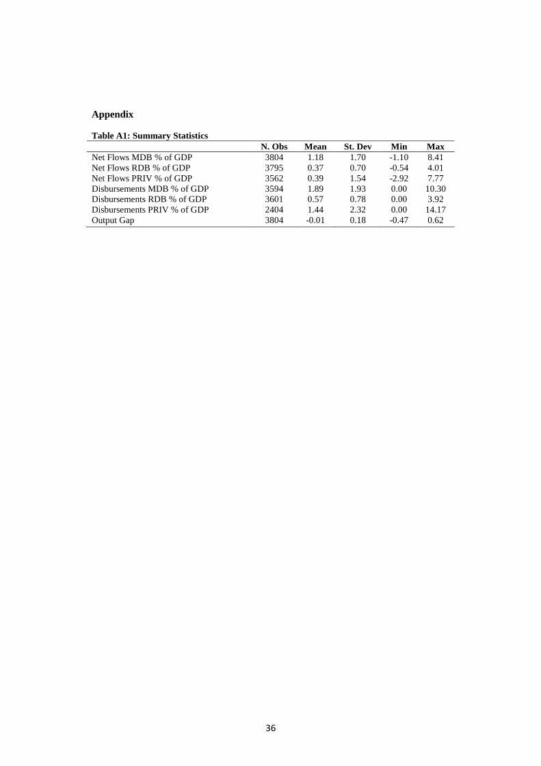
Appendix

Table A1: Summary Statistics

N. Obs Mean St. Dev Min Max

Net Flows MDB % of GDP 3804 1.18 1.70 -1.10 8.41

Net Flows RDB % of GDP 3795 0.37 0.70 -0.54 4.01

Net Flows PRIV % of GDP 3562 0.39 1.54 -2.92 7.77

Disbursements MDB % of GDP 3594 1.89 1.93 0.00 10.30

Disbursements RDB % of GDP 3601 0.57 0.78 0.00 3.92

Disbursements PRIV % of GDP 2404 1.44 2.32 0.00 14.17

Output Gap 3804 -0.01 0.18 -0.47 0.62

Documents

The Cyclicality of International Public Sector Borrowing ...repec.graduateinstitute.ch/pdfs/Working_papers/HEIDWP17-2017.pdf · each other leading to a “when it rains it pours”