.Numerical Analysis ProjectManuscript NA-87-01

. February 1987

.

The Convergence of Inexact Chebyshevand Richardson Iterative Methods for Solving

Linear Systems

Gene H. GolubMichael L. Overton

Numerical Analysis ProjectComputer Science Department

Stanford UniversityStanford, California 94305

,.

THE CONVERGENCE OF INEXACT CHEBYSHEVAND RICHARDSON ITERATIVE METHODS FOR SOLVING

LINEAR SYSTEMS

Gene H. Golub* and Michael L. Overton**

(Also issued on a report from the Centre for Mathematical Analysis,Canberra, Australia - CMA-R46-86)

February 1987

* Computer Science Department, Stanford University, Stanford, CA 94305(Golub at SCORE.Stanford,edu). The work of this author was in partsupported by the NSF (DCR 84-12314) and by the U.S. Army (WAG 298%K-0124).

**Centre for Mathematical Analysis and Mathematical Sciences ResearchInstitute, Australian National University. (On leave from CourantInstitute of Mathematical Sciences, New York University.)(NA Overton at SCORE.Stanford,edu) The work of this author was in .part supported by NSF (DCR-85-02014).

The Chebyshev and second-order Richardson methods are classical

iterative schemes for solving linear systems. We consider the

convergence analysis of these methods when each step of the iteration is

carried out inexactly. This has many applications, since a

preconditioned iteration requires, at each step, the solution of a

linear system which may be solved inexactly using an “inner” iteration.

. We derive an error bound which applies to the general nonsymmetric

inexact Chebyshev iteration. We show how this simplifies slightly in

the case of a synunetric or skew-symmetric iteration, and we consider

both the cases of underestimating and overestimating the spectrum. We

show that in the symmetric case, it is actually advantageous to

underestimate the spectrum when the spectral radius and the degree of

inexactness are both large. This is not true in the case of the

skew-symmetric iteration. We show how similar results apply to the

Richardson iteration. Finally, we describe numerical experiments which

illustrate theresults and suggest that the Chebyshev and Richardson

methods, with reasonable parameter choices, may be more effective than

the conjugate gradient method in the presence of inexactness.

2

1.. INlmDumIoN *

The Chebyshev method and the second-order Richardson methods are

classical iterative schemes for the solution of linear systems of

equations. Iheir convergence analysis is well known; see Golub and

Varga (1961). We consider the analysis of these methods where each step

of the iteration is carried out inexactly. This has important

applications, since one often wants to employ a matrix splitting,

introducing a linear system to be solved at each step of the main or

“outer” iteration. When the exact solution of these “inner” systems is

not possible or practical, an “inner” iteration may be used instead.

These ‘inner iterations are generally terminated before they have

converged to full accuracy: in other words the inner systems are solved

inexactly. We are concerned with the effect this has on the convergence

of the outer iteration.

Other papers which study the use of inner and outer iterations

include Gunn (1964). Nicolaides (1975). Pereyra (1967), Nichols (1973)

and Dembo. Eisenstat and Steihaug (1982). In an earlier paper (Golub

and Overton (1982)) we gave a convergence analysis for the inexact

Richardson method alone, but the analysis there is somewhat different

since it does not take advantage of the freedom of choice in the initial

i terates. The analysis given here is also applicable to studying

round-off error accumulation; see also Golub (1962).

The paper is organized as follows. In Section 2 we give a general

convergence analysis for the inexact Chebyshev method for solving non-

symmetric linear systems. The exact version of this method is the one

given by Manteuffel (1977). We give the analysis for the nonsymmetric.

case because it is not much more complicated than the symmetric version.

3

In Section 3 we show how the results apply to the symmetric iteration,

distinguishing between the cases where the relevant eigenvalues are

“underestimated” and “overestimated”. We show that underestimating the

spectrum can actually speed up convergence if the spectral radius is

large and the iteration is quite inexact. In Section 4 we apply the

results of Section 2 to the case where the preconditioned matrix

defining the outer system is the sum of the identity matrix and a

skew-symmetric matrix. We refer to the corresponding iteration as

“skew-symmetric”. This situation provides one motivation for our work,

since it arises as an effective way to solve nonsymmetric systems with

positive definite symmetric part, using a skew-symmetric/symmetric

splitting. Again. we discuss the issue of overestimating and

underestimating the spectrum.

In Section 5 we give a convergence analysis for the inexact second-

order Richardson method, restricting it for simplicity to the case of a

symmetric iteration where the spectrum is overestimated. The second-

order Richardson method is closely related to the SOR method; see Golub

and Varga (1961, p.151). In Section 6 we discuss the question of how to

choose the parameters to minimize the total amount of work.

It seems to be much more difficult to provide a similar analysis

for the conjugate gradient method. However, numerical results given in

the final section indicate that the Chebyshev and Richardson methods,

with reasonable parameter choices, are less sensitive than the conjugate

gradient method to the degree of inexactness of the iteration.

We use II*II to denote the Euclidean vector and induced matrix

norm. Unless otherwise specified, a statement involving k will be

understood to apply for k = 0.1.2.... .

4

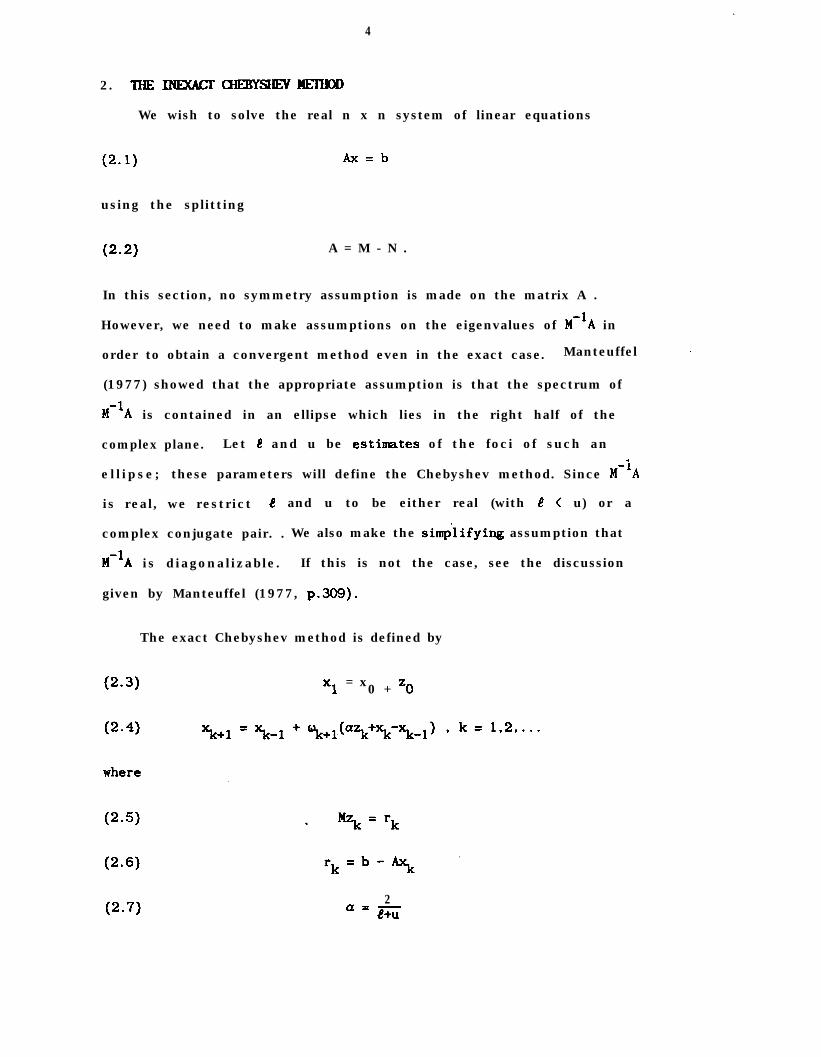
2. lHElNExAcr~sHEvHElHoD

We wish to solve the real n x n system of linear equations

(2.1) Ax=b

using the splitting

(2*2) A = M - N .

In this section, no symmetry assumption is made on the matrix A .

However, we need to make assumptions on the eigenvalues of M’lA in

order to obtain a convergent method even in the exact case. Manteuffel

(1977) showed that the appropriate assumption is that the spectrum of

M-lA is contained in an ellipse which lies in the right half of the

complex plane. Let e and u be estinrates of the foci of such an.

ellipse; these parameters will define the Chebyshev method. Since M-‘A

is real, we restrict e and u to be either real (with 4 < u) or a

complex conjugate pair. . We also make the simplifying assumption that

M’lA is diagonalizable. If this is not the case, see the discussion

given by Manteuffel (1977, p.309).

The exact Chebyshev method is defined by

(2-3) x1 = x0 + z.

=b- %c.

‘k

2a=&+u

5

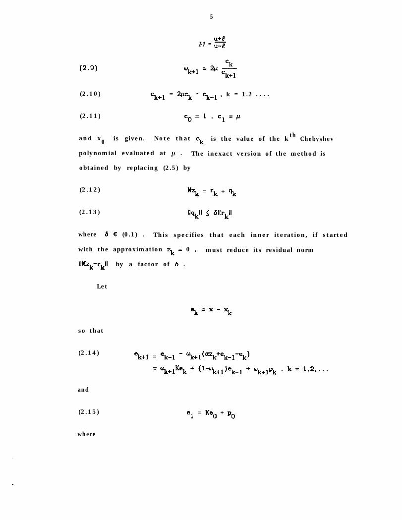
u+l??I-1 = u-e

(2.9)

(2.10) ck+l = 2pck - c.,-~ , k = 1.2 ,...

‘ky<+l =*-

ck+l

(2.11) co=1.c1=&4

and x0 is given. Note that ck is the value of the kth Chebyshev

polynomial evaluated at p . The inexact version of the method is

obtained by replacing (2.5) by

(2.12) “\ = ‘k + qk

(2.13) llqkll < 611rkll

where 6 E (0.1) . This specifies that each inner iteration, if started

with the approximation zk = 0 , must reduce its residual norm

II%-rkll by a factor of 6 .

Let

so that

(2.14)

and

(2.15)

where

ek+l = ek-l - ~+l(a~+~-l-ek)

el = Keo + p.

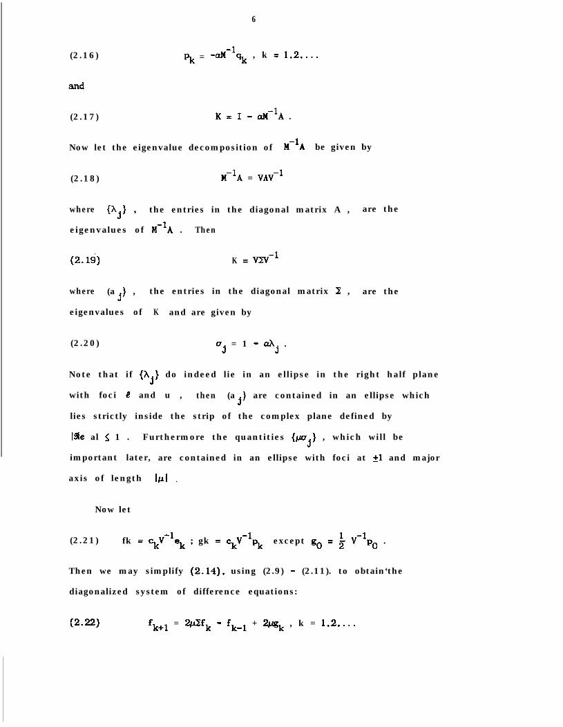
(2.16) pk = -aM-‘qk , k = 1,2,...

6

(2.17) K=I - aM-lA .

Now let the eigenvalue decomposition of M-'A be given by

(2.18) M-lA = WV-’

where{'j) ’ the entries in the diagonal matrix A , are the

eigenvalues of M-lA . Then

(2.19) K = m-l

where (a } ,J

the entries in the diagonal matrix Z , are the

eigenvalues of K and are given by

(2.20) aj = 1 - dj .

Note that if (Aj} do indeed lie in an ellipse in the right half plane

with foci 4 and u , then (a } are contained in an ellipse whichJ

lies strictly inside the strip of the complex plane defined by

It&e al < 1 . Furthermore the quantities {b,} , which will be

important later, are contained in an ellipse with foci at 21 and major

axis of lengthIp I l

Now let

(2.21) fk = ckV-‘ek ; gk = ckV-‘pk except go = a VW1po .

Then we may simplify (2.14), using (2.9) - (2.11). to obtain‘the

diagonalized system of difference equations:

(2.221 fk+1 = wfk - fk-1 + wk , k = 1,2....

7

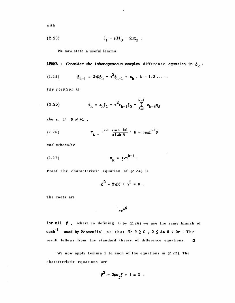
with

(2-W

We now state a useful lemma.

LEUMA 1 Constder the tnhosnogeneous complex difference equation tn Sk :

(2.24) rk+l = 27Pek - 72fk-1 + x , k = 1.2 ,... .

T h e s o l u t i o n i s

k-l

(2.26) Tk = 7k-l sinh ke , 8 - cash-$3sinh8 -

a n d o t h e r w i s e

(2.27) = +kTk-l .=k -

,

Proof The characteristic equation of (2.24) is

P2 - 27/3f + T2 = 0 .

The roots are

forall p, where in defining 8 by (2.26) we use the same branch of

cash-1 usedbyManteuffe1, so that 9e0>0, 0<9ar8<2n. The

result follows from the standard theory of difference equations. o

We now apply Lemma 1 to each of the equations in (2.22). The

characteristic equations are

P2 -*J3:+1=o-

8

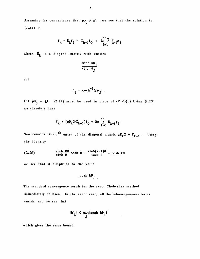
Assuming for convenience that pj # +l , we see that the solution to

(2.22) is

k- lfk = Dkfl - Dkwlfo + 2p 1 D ge 1 k-4 4=

where Dk is a diagonal matrix with entries

sinh ke.

zGidj

and

eJ = cash-‘(wj) .

(If wj = 21 . (2.27) must be used in place of (2.26).) Using (2.23)

we therefore have

k-l

Now corisider the j th entry of the diagonal matrix pDkZ - Dl-l . Using

the identity

(2-W sinh kesi*e COSh0- si*(k-l)e = co& kesinh 8

we see that it simplifies to the value

. cash kf35 l

The standard convergence result for the exact Chebyshev method

immediately follows. In the exact case, all the inhomogeneous terms

vanish, and we see tha’t

llfkll < llEU&osh kejlJ .

which gives the error bound

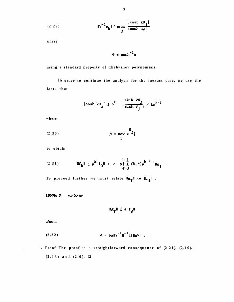
(2.29)

where

9

IIV-lekll < maxj kg6

JI= cash-‘p

using a standard property of Chebyshev polynomials.

In order to continue the analysis for the inexact case, we use the

facts that

lcoshke I <pk sinh kt3.

j, I < kpk-’sinhe -

j I

where

(2.30)

to obtain

k-l(2.31) llfkll < pkllfoll + 2 l/L] 1 (k-C)pk-e-lllgell .

e=o

P = maxleejI.j

To proceed further we must relate llgell to lIfeI .

LEHA2

where

(2.32)

llgell $ allfell

We have

6= &llV-lM-l II IIAVII .

. . Proof The proof is a straightforward consequence of (2.21). (2.16).

(2.13) and (2.6). q

10

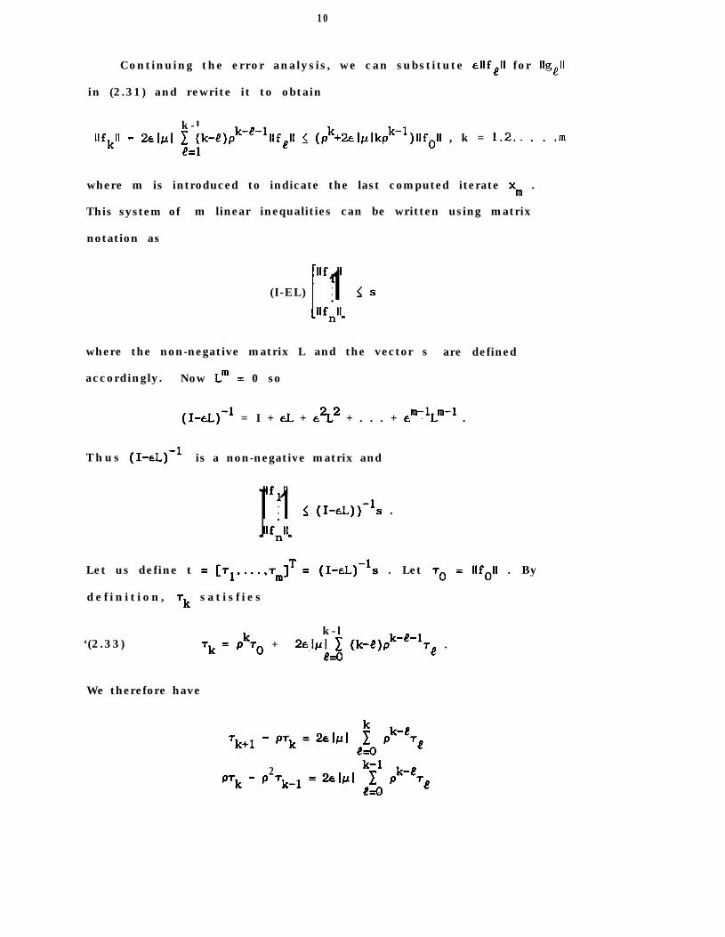
Continuing the error analysis, we can substitute elIfell for llgell

in (2.31) and rewrite it to obtain

k-lllfkll - 244 1 (k-t)pk-e-lllfell < (pk+2elplkpk-1)llfoll , k = 12.. . . ,m

i?=l

where m is introduced to indicate the last computed iterate xm .

This system of m linear inequalities can be written using matrix

notation as

(I-EL)

Ilf $1.1 1. IS

llfnll

where the non-negative matrix L and the vector s are defined

accordingly. Now L” = 0 so

(I-& = I + EL + A2 + . . . + Em-lLm-l .

Thus (I-eL)-l is a non-negative matrix and

Ilf $1.I 1. < (I-rL))% .

llfnll

Let us define t = [T,.....T,]~ = (I-eL)-‘s . Let ~~ = llfOll . By

definit ion, rk satisf ies

‘(2.33)k- l

rk = pk~o + 244 1 (k-4!)pk-e-1,e .e=o

We therefore have

2pTk - p rk-1

11

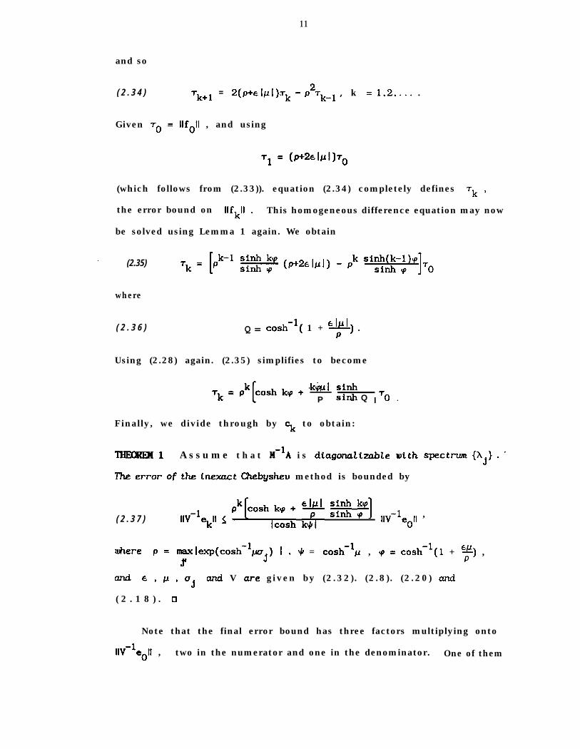
and so

( 2 . 3 4 ) Tk+l = 2(P+EICII)irk - p2~k-l , k = 1.2.... .

Given 7O = llfOll , and using

Tl = (p+2E;I111)To

(which follows from (2.33)). equation (2.34) completely defines Tk ’

the error bound on llfkll . This homogeneous difference equation may now

be solved using Lemma 1 again. We obtain

( (2.35)

where

( 2 . 3 6 ) Q = cash-‘( 1 + e+) .

Using (2.28) again. (2.35) simplifies to become

rk+I sinhkcp

P sinh Q I To l

Finally, we divide through by ck to obtain:

TEEOREXl A s s u m e t h a t M'lA i s diagonalizable luCth spectrum {hj} . -

The error of the tnexuct Chebysheu method is bounded by

( 2 . 3 7 ) IIv-lekll < $oshlzsh Y$ ::z 71 IIv-leoll ,

where p = -bp(co&mj) I . \CI = cash-‘p , Q = cashJ

-+1 + E+) ,

and c,p.uj cud V are given by (2.32). (2.8). (2.20) and

( 2 . 1 8 ) . (3

Note that the final error bound has three factors multiplying onto

IIV-‘eoll , two in the numerator and one in the denominator. One of them

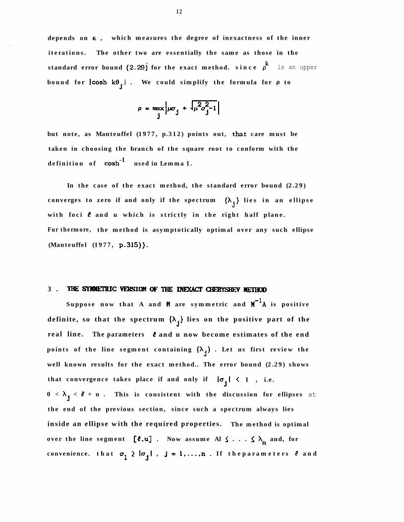
12

depends on e , which measures the degree of inexactness of the inner

iterations. The other two are essentially the same as those in the

standard error bound (2.29j for the exact method. s ince pk is an upper

bound for lcosh k0.I .J

We could simplify the formula for p to

but note, as Manteuffel (1977, p.312) points out, .that care must be

taken in choosing the branch of the square root to conform with the

definition of cash-1 used in Lemma 1.

In the case of the exact method, the standard error bound (2.29)

converges to zero if and only if the spectrum (X } lies in an ellipsej

with foci 4 and u which is strictly in the right half plane.

Fur thermore, the method is asymptotically optimal over any such ellipse

(Manteuffel (1977, p.315)).

3 . -lHESWHEIRICVEl?SIONOFTIIEINEXA~~HEIHOD

Suppose now that A and M are symmetric and M’lA is positive

definite, so that the spectrum {Aj) lies on the positive part of the

real line. The parameters e and u now become estimates of the end

points of the line segment containing (x,} . Let us first review the

well known results for the exact method.. The error bound (2.29) shows

that convergence takes place if and only if lajl < 1 , i.e.

0 < hj < e + u . This is consistent with the discussion for ellipses at

the end of the previous section, since such a spectrum always lies

inside an ellipse with the required properties. The method is optimal

over the line segment ☯& u) l Now assume Al 5 . . . < hn and, for

convenience. that crl 1 Iojl , j=l....,n. I f theparameters 4? and

13

U overestimate the spectrum, i.e. e<hl’hn<U’ then the

numerator of the standard error bound (2.29) is less that one and may be

written

(3.1) cos k COS-‘(/JU~)

since wl < 1 and tJl is imaginary. The optimal

parameters is well known to be e = A1 , u = hn ,

numerator of one in (2.29).

Now consider the inexact method. The analysis of the previous

choice of the

which gives a

section simplifies slightly, since the matrix V of (2.18) may be

written

(3.2) V = M-l’%

where v is orthogonal. The quantity e in (2.32) simplifies

accordingly. Otherwise there are no changes, and we obtain:

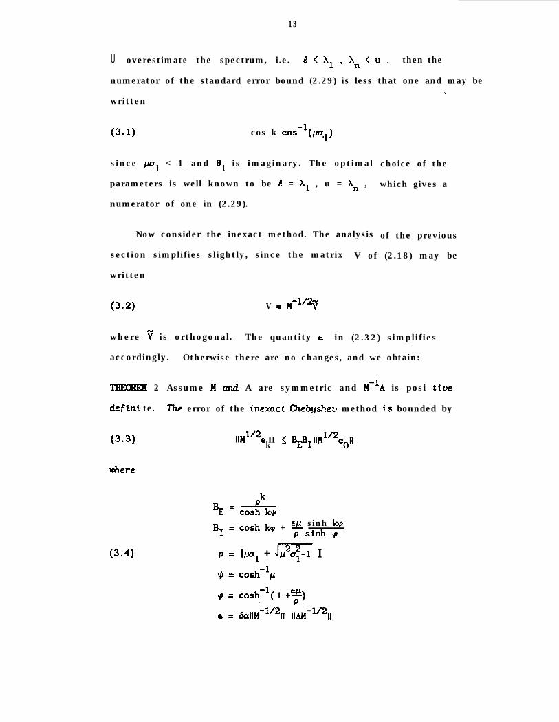
THEloREI1 2 Assume M and A are symmetric and M’lA is posi tiue

&fCni te. The error of the tnexact Chebysheu method ts bounded by

(3=31

where

P-4)

BE =BI =

P =

cp=& =

lllP2e IIk < BEBI llM1’2e011

pkcash k$

cash kp + ~11, sinh kqP sinh cp

lPl + Jq I

cash-‘l,l

cash-‘( 1 +‘f)

6all!J+~211 llAM-1’211

14

and p,a,ul. are given by (2.8). (2.7) and (2.20). ruith

a1 2 10j I l 0

(Note that we have introduced notation BR and BI for the exact and

inexact factors in the error bound, and we have simplified the formulas

for p and e .)

Now let us assume that Al + An is known and that

e+u = A1 + An . Since the centre of the spectrum is fixed by this

assumption, a in (2.7) has the correct value and so al = -0 I. Withn

a fixed, the iteration depends only on the parameters p and 6 .

Note that in the limit, as p +Q) , the Chebyshev method becomes the

first-order Richardson method, which is closely related to the

Gauss-Seidel method. We have already mentioned that in the exact case,

i .e . when 6 = 0 , the optimal value is given by ~1 = 1 , i.e.

p = l/u1 . -It is now quite instructive to examine the error bound (3.3)

to see how to choose the optimal value of p if 6 > 0 .

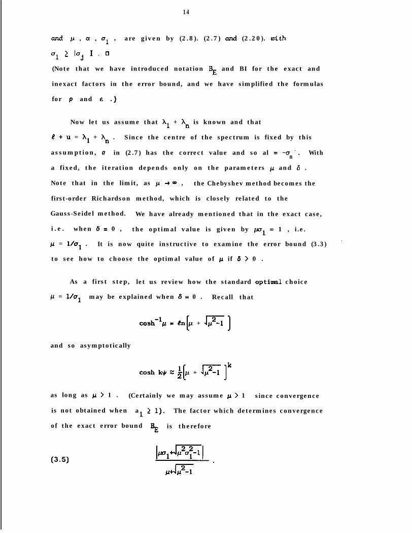
As a first step, let us review how the standard op’timal choice

p = l/u1 may be explained when 6 = 0 . Recall that

cash-lp = en[p + &]

and so asymptotically

cash k+‘z gl + qk

as long as p > 1 . (Certainly we may assume p > 1 since convergence

is not obtained when a1 1 1). The factor which determines convergence

of the exact error bound BE is therefore

(34

15

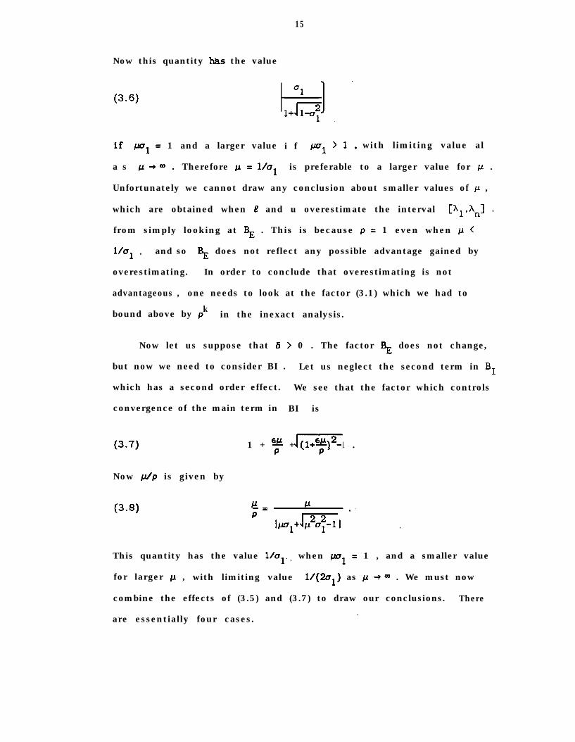
Now this quantity &s the value

O-6)

if WI = 1 and a larger value i f IJol>l. with limiting value al

a s ~+a. Therefore Jo = l/al is preferable to a larger value for ~1 .

Unfortunately we cannot draw any conclusion about smaller values of p ,

which are obtained when e and u overestimate the interval C?p,l ’from simply looking at BE . This is because p = 1 even when ~1 <

l/a1 . and so + does not reflect any possible advantage gained by

overestimating. In order to conclude that overestimating is not

advantageous , one needs to look at the factor (3.1) which we had to

kbound above by p in the inexact analysis.

Now let us suppose that 6 > 0 . The factor BE does not change,

but now we need to consider BI . Let us neglect the second term in BI

which has a second order effect. We see that the factor which controls

convergence of the main term in BI is

(3.7)

Now /.dp is given by

1 + e: + (l+$ -1 .r

This quantity has the value l/al.. when ~1 = 1 , and a smaller value

for larger ~1 , with limiting value 1/(2ol) as p +Q) . We must now

combine the effects of (3.5) and (3.7) to draw our conclusions. There

are essentially four cases..

16

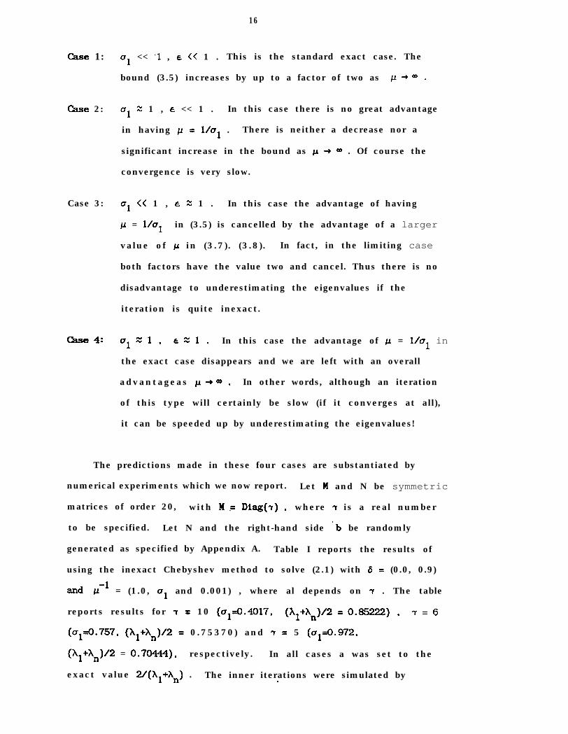
G.se 1:

Case 2:

Case 3:

tkse 4:

a1 << -1 , e << 1 . This is the standard exact case. The

bound (3.5) increases by up to a factor of two as p+a.

a1 z 1 , e << 1 . In this case there is no great advantage

in having p = l/al . There is neither a decrease nor a

significant increase in the bound as p + a . Of course the

convergence is very slow.

a1 << 1 , d z 1 . In this case the advantage of having

p = l/C71 in (3.5) is cancelled by the advantage of a larger

value of p in (3.7). (3.8). In fact, in the limiting case

both factors have the value two and cancel. Thus there is no

disadvantage to underestimating the eigenvalues if the

iteration is quite inexact.

UlZl, EZl. In this case the advantage of p = l/al in

the exact case disappears and we are left with an overall

advantageas ~+a. In other words, although an iteration

of this type will certainly be slow (if it converges at all),

it can be speeded up by underestimating the eigenvalues!

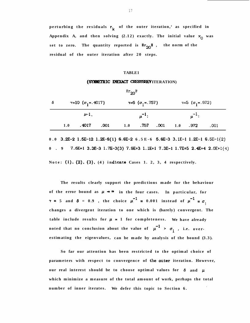
The predictions made in these four cases are substantiated by

numerical experiments which we now report. Let M and N be symmetric

matrices of order 20, with M t Diag(r) ,’ where 7 is a real number

to be specified. Let N and the right-hand side ‘b be randomly

generated as specified by Appendix A. Table I reports the results of

using the inexact Chebyshev method to solve (2.1) with 6 = (0.0, 0.9)

and P-l = (1.0, 01 and 0.001) , where al depends on 7 . The table

reports results for 7 = 10 (crl~O.4017, (h1+$)” =0.85222), 7=6

(ul=O.757. (X1+Xn)/2 = 0.75370) and 7 = 5 (alzO.972,

(X1+Jp = 0.70444). respectively. In all cases a was set to the

exact value 2/(hl+A,) . The inner iterations were simulated bys

17

perturbing the residuals rk of the outer iteration,‘ as specified in

Appendix A, and then solving (2.12) exactly. The initial value x0 was

set to zero. The quantity reported is IIrZOll , the norm of the

residual of the outer iteration after 20 steps.

TABLE1

(SYHHETRIC INIzAcr QIEB’YSIEV ITERATION)

IIr2011

6 -r=lO (u1=.4017) r=6 (u1=.757) d5 (u1=.972)

Ir -1. lP

-1 : -1 :

P

1.0 .4017 .OOl 1.0 .757 .OOl 1.0 .972 ,001

0 . 0 3.2E-2 1.5E-12 1X-8(1) 8.8E-2 6 . 5 E - 6 5.8E-3 3.1E-1 1.2E-1 8.5E-l(2)

0 . 9 7.6E+l 3.3E-3 1X-3(3) 7.9E+3 l.lE+l 7.3E-1 1.7E+5 2.4E+4 2.OE+1(4)

Note: (1). (2). (3). (4) i d’n icate Cases 1. 2, 3, 4 respectively.

The results clearly support the predictions made for the behaviour

of the error bound as p +a in the four cases. In particular, for

7 = 5 and 6 = 0.9 , the choice r-;-l = 0.001 instead of p-l =u1changes a divergent iteration to one which is (barely) convergent. The

table include results for p = 1 for completeness. We have already

noted that no conclusion about the value of p-’ > aI , i.e. over-

estimating the eigenvalues, can be made by analysis of the bound (3.3).

So far our attention has been restricted to the optimal choice of

parameters with respect to convergence of the.outer iteration. However,

our real interest should be to choose optimal values for 6 and p

which minimize a measure of the total amount of work, perhaps the total

number of inner iterates. We defer this topic to Section 6..

18

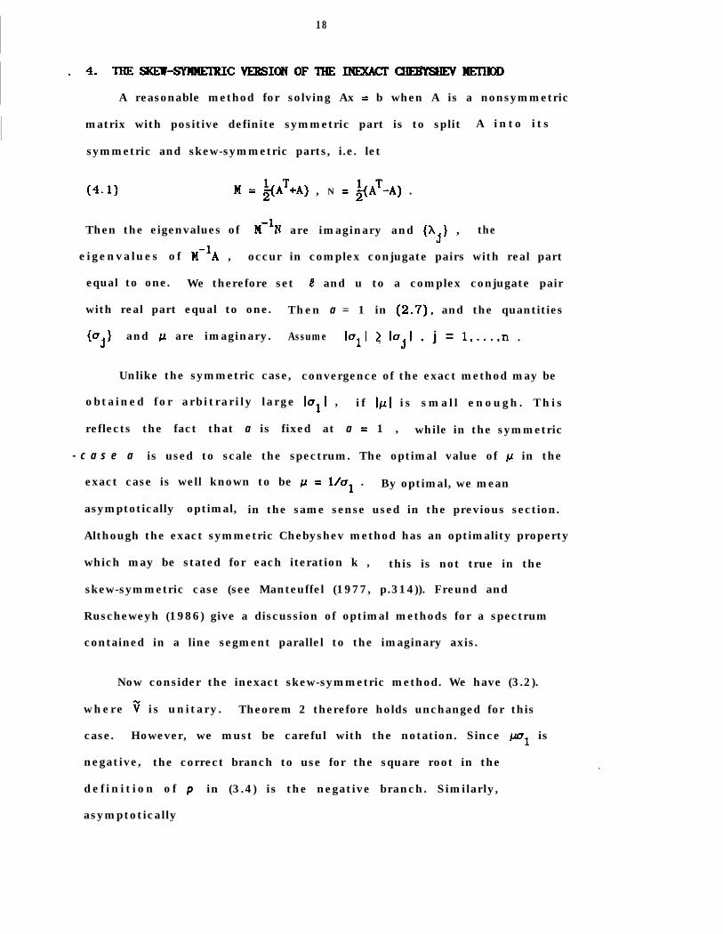
. 4.THESKEV-SYHMEIRICVERSIONOFlHEMExkc=TcHElfysHEv~~

A reasonable method for solving Ax = b when A is a nonsymmetric

matrix with positive definite symmetric part is to split A into its

/ symmetric and skew-symmetric parts, i.e. let

(4-l) M = $(A,A) , N = $A~-A) .

Then the eigenvalues of M-lN are imaginary and {hj) , the

eigenvalues of M-lA , occur in complex conjugate pairs with real part

equal to one. We therefore set 4 and u to a complex conjugate pair

with real part equal to one. Then a = 1 in (2.7), and the quantities

I”jI and p are imaginary. Assume $1 2 lujl . j = l,...,n .

Unlike the symmetric case, convergence of the exact method may be

obtained for arbitrarily large lull , if IpI is small enough. This

reflects the fact that a is fixed at a = 1 , while in the symmetric

- c a s e a is used to scale the spectrum. The optimal value of p in the

exact case is well known to be p = l/al . By optimal, we mean

asymptotically optimal, in the same sense used in the previous section.

Although the exact symmetric Chebyshev method has an optimality property

which may be stated for each iteration k , this is not true in the

skew-symmetric case (see Manteuffel (1977, p.314)). Freund and

Ruscheweyh (1986) give a discussion of optimal methods for a spectrum

contained in a line segment parallel to the imaginary axis.

Now consider the inexact skew-symmetric method. We have (3.2).

where v is unitary. Theorem 2 therefore holds unchanged for this

case. However, we must be careful with the notation. Since l-(ol is

negative, the correct branch to use for the square root in the

definition of p in (3.4) is the negative branch. Similarly,

asymptotically

.

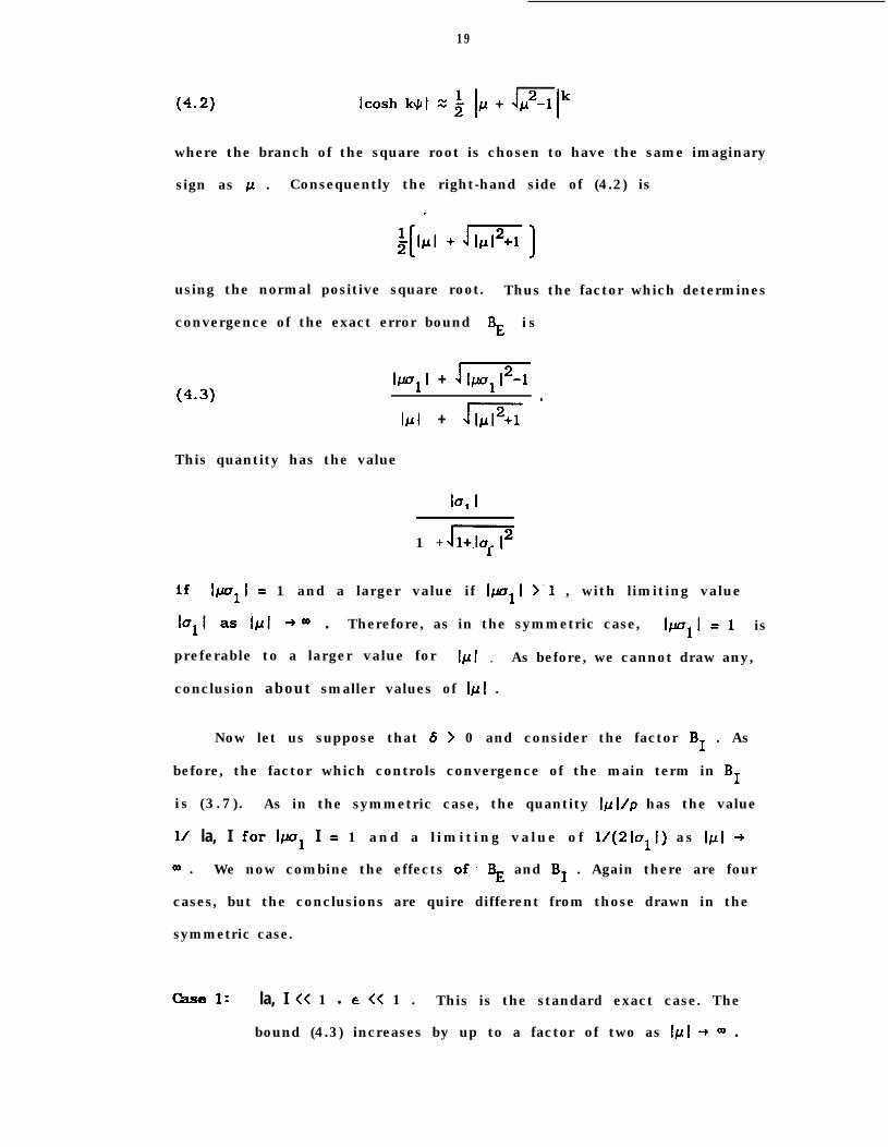
19

where the branch of the square root is chosen to have the same imaginary

sign as p . Consequently the right-hand side of (4.2) is

using the normal positive square root. Thus the factor which determines

convergence of the exact error bound BE is

(4-3)IPq + 11,,12-1

Id + llr12+1 -

This quantity has the value

la, I

1 + l+lul I7

if Iw,l = 1 and a larger value if 1~~1 >‘l , with limiting value

I=+ 8s Ij.4 +a . Therefore, as in the symmetric case, lP1 l =l is

preferable to a larger value for lpl l As before, we cannot draw any,

conclusion about smaller values of Ij.fI .

Now let us suppose that 6 > 0 and consider the factor BI . As

before, the factor which controls convergence of the main term in BI

is (3.7). As in the symmetric case, the quantity lpi/p has the value

11 la, I for lpo1 I = 1 and a limiting value of 1/(21ull) as 1~~1 +

QD . We now combine the effects of. s and BI . Again there are four

cases, but the conclusions are quire different from those drawn in the

symmetric case.

&se I: la, I << 1 l E << 1 . This is the standard exact case. The

bound (4.3) increases by up to a factor of two as lpl + Q) .

20

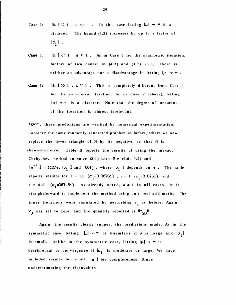
Case 2:

&se 3:

&se 4:

la, I >> 1 , E << 1 . In this case letting Ir.rl + a is a

disaster. The bound (4.3) increases by up to a factor of

Ia+ -

la, I << 1 , d 2 1 . As in Case 3 for the symmetric iteration,

factors of two cancel in (4.3) and (3.7). (3.8). There is

neither an advantage nor a disadvantage in letting 1~1 + 0~ .

la, I >> 1 , d 2 1 . This is completely different from Case 4

for the symmetric iteration. As in Case 2 (above), letting

lpl -)a is a disaster. Note that the degree of inexactness

of the iteration is almost irrelevant.

bin, these predictions are verified by numerical experimentation.

Consider the same randomly generated problem as before, where we now

replace the lower triangle of N by its negative, so that N is

- skew-symmetric. Table II reports the results of using the inexact

Chebyshev method to solve (2.1) with d = (0.0, 0.9) and

lp-’ I = (1017, la, I and .OOl) , where la, I depends on 7 . The table

reports results for 7 = 10 (u =0.3676i)1 , 7 = 1 (a =3.676f)1 and

7 = 0.01 (01=367.61) . As already noted, a = 1 in ill cases. It is

straightforward to implement the method using only real arithmetic. The

inner iterations were simulated by perturbing rk as before. Again,

x0 was set to zero, and the quantity reported is llr2011 .

Again, the results clearly support the predictions made. As in the

symmetric case, letting l&d --)O” is harmless if 6 is large and lull

is small. Unlike in the symmetric case, letting 1~1 + a is

detrimental to convergence if lull is moderate or large. We have

included results for small I/L I for completeness. Since

underestimating the eigenvalues

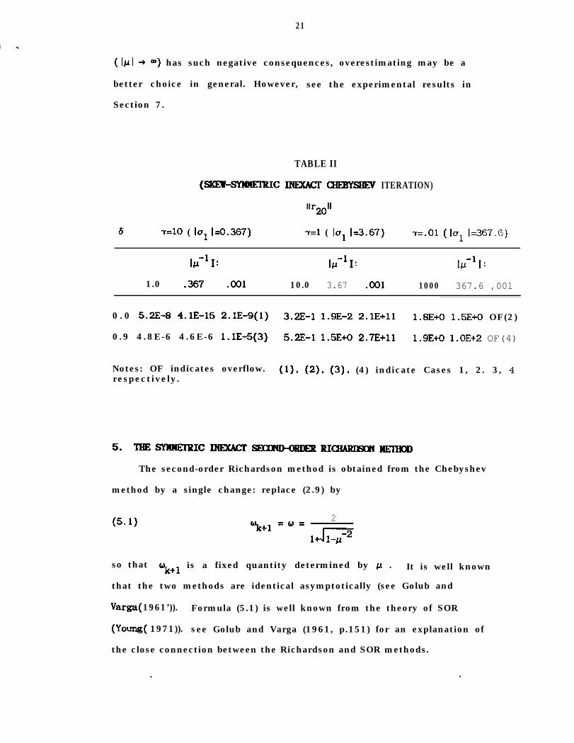
21

(Ipl + a) has such negative consequences, overestimating may be a

better choice in general. However, see the experimental results in

Section 7.

6

TABLE II

(SKEW-m1c llmrAcr c3amaEv ITERATION)

II r2011

7=10 ( la, 1=0.367) r=l ( la, 1=3.67) ~=.01 (la, k367.6)

l/l--l I : ICC-’ I : I/l--‘I:

1.0 .367 .OOl 10.0 3.67 .OOl 1000 367.6 ,001

0.0 5.2E-8 4.1E-15 2.1E-9(l) 3.2E-1 1.9E-2 2.1E+ll 1.8E+O 1.5E+O OF(2)

0.9 4.8E-6 4.6E-6 l.lE-5(3) 5.2E-1 1.5E+O 2.7E+ll 1.9E+O l.OE+2 OF(4)

Notes: OF indicates overflow. (1). (2). (3). (4) indicate Cases 1, 2. 3, 4respectively.

5.ImEsnmErRIc INExAcr-RI~wEIHoD

The second-order Richardson method is obtained from the Chebyshev

method by a single change: replace (2.9) by

(5.1) ok12

+ =&I=1+p

so that ok+1 is a fixed quantity determined by p . It is well known

that the two methods are identical asymptotically (see Golub and

Varga( 1961’)). Formula (5.1) is well known from the theory of SOR

(Young( 1971)). see Golub and Varga (1961, p.151) for an explanation of

the close connection between the Richardson and SOR methods.

22

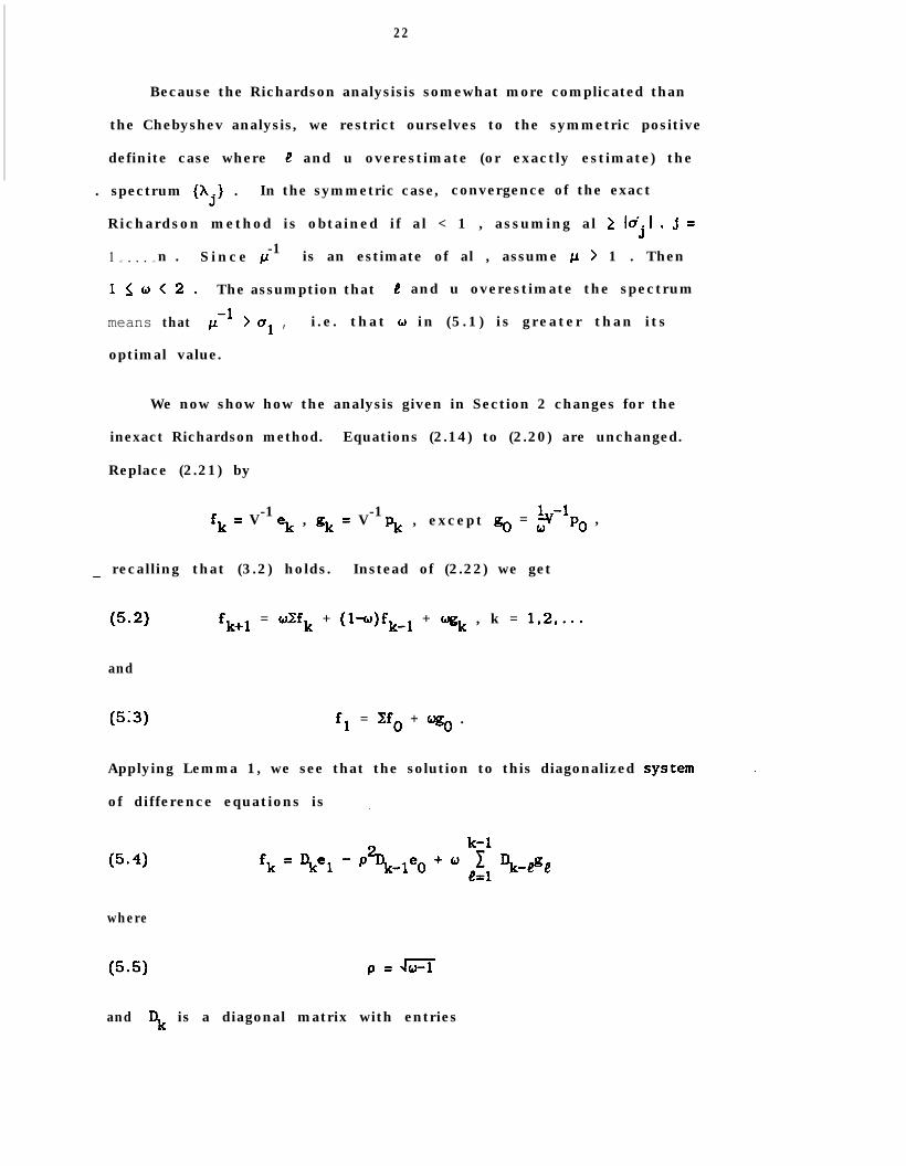
Because the Richardson analysisis somewhat more complicated than

the Chebyshev analysis, we restrict ourselves to the symmetric positive

definite case where +? and u overestimate (or exactly estimate) the

. spectrum {Xj} . In the symmetric case, convergence of the exact

Richardson method is obtained if al < 1 , assuming al 2 luil , j =

1 Since ~1-1. l l l , n . is an estimate of al , assume fi > 1 . Then

1<0<2. The assumption that 4 and u overestimate the spectrum

means that -lp > a1 , i.e. that 0 in (5.1) is greater than its

optimal value.

We now show how the analysis given in Section 2 changes for the

inexact Richardson method. Equations (2.14) to (2.20) are unchanged.

Replace (2.21) by

-1fk = V ek , gk = V-1pk , except go = $f-‘po ,

_ recalling that (3.2) holds. Instead of (2.22) we get

(5.2)

and

fk+l = UZfk + (lw)fk-1 + wgk , k = 1,2,...

(5i3) fl = Zfo + @go .

Applying Lemma 1, we see that the solution to this diagonalized system

of difference equations is _

.

(5.4) fk=vl-P

where

(5.5) p=G=i

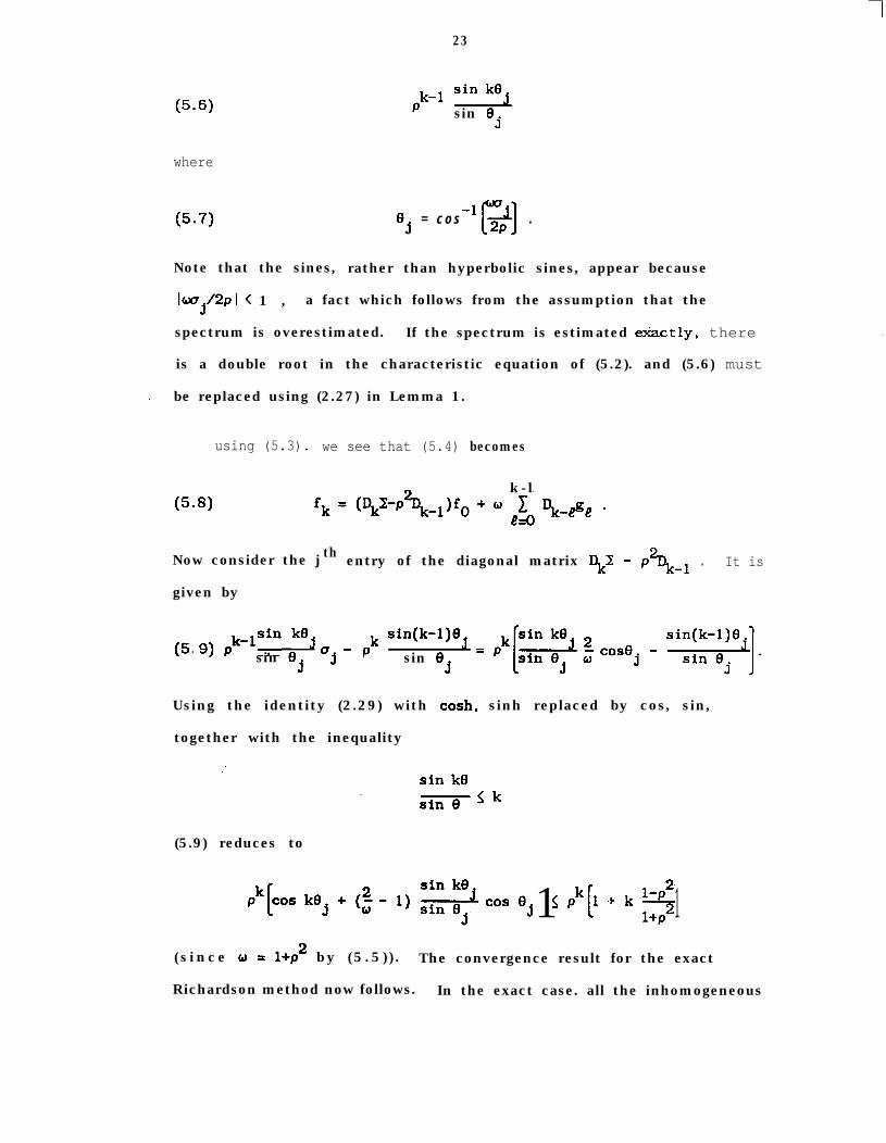
and Dk is a diagonal matrix with entries

23

(5.6)

where

sinsin 8

j

%= c o s-‘+ .PI

Note that the sines, rather than hyperbolic sines, appear because

IWj”PI < 1 , a fact which follows from the assumption that the

spectrum is overestimated. If the spectrum is estimated exactly, there

is a double root in the characteristic equation of (5.2). and (5.6) must

G be replaced using (2.27) in Lemma 1.

using (5.3). we see that (5.4) becomes

(5-8)k-l

Now consider the j th entry of the diagonal matrix Dkl - p%-k 1 . It is

given by

t5 gj pk-lsin kej k sin(k-1)8.. sin 8 =j - P sin 8

J = pk -J J 5

Using the identity (2.29) with cash, sinh replaced by cos, sin,

together with the inequality

(5.9) reduces to

j1 [< pk 1 + k 1-p2l+p21

(s ince o = l+p2 by (5.5) ) . The convergence result for the exact

Richardson method now follows. In the exact case. all the inhomogeneous

24

terms in (5.8) vanish, and we see that

llM1’2 $ pk2

ekll 1 + k 9 llM1’2eolll+P 3

which is the bound given by Golub (1959, p-23).

For the analysis of the inexact case we need now to relate llgeli

to lIfeI . Lemma 2 applies, showing that

llgell < rllfell

where

(5.10) tz = &llM-1’211 IIAM-1’211 .

We can therefore substitute rllfell for llgell in (5.8) to obtain

llfkll 5 pk 1 +[

The same argument used

consequently ,

2

I

k- lk’% llfOll + oe 1 (k-4?)pk-e-111fell .

l+P e=o

in the Chebyshev analysis shows that,

llfkll < Tk

where

2 k- lt5-11) Tk = pk[l + k *], + e 1 (kee)pk-e-l,e ,

l+p2 .O eye

Using the same technique as before, we see that 7k satisfies

(5.12)

We also have .

(5.13) Tl = [P[l + =J ++.

25

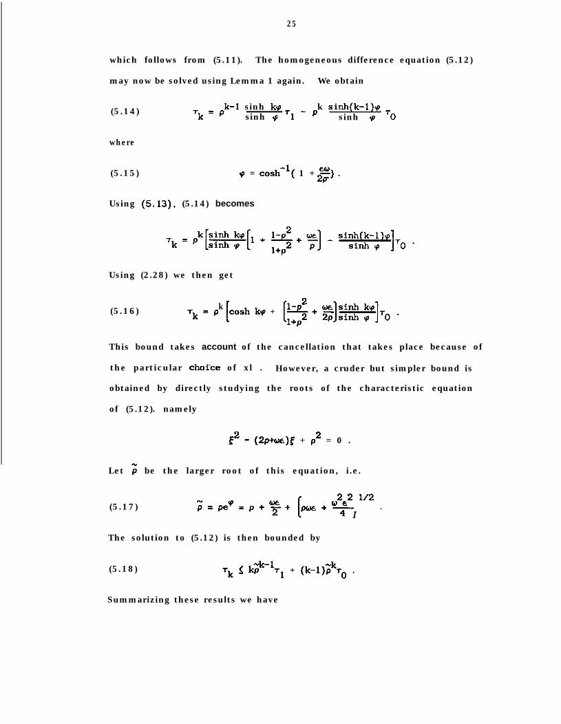
which follows from (5.11). The homogeneous difference equation (5.12)

may now be solved using Lemma 1 again. We obtain

(5.14)

where

(5.15)

rk= pk-l sinh kp

sinh cp rl - pk sinh(k-l)v

sinh cp TO

cp = cash-‘( 1 + =) .2P

Using (5.13), (5.14) becomes

Using (2.28) we then get

(5.16) krk = p cash kq +

This bound takes account of the cancellation that takes place because of

the particular choi‘ce of xl . However, a cruder but simpler bound is

obtained by directly studying the roots of the characteristic equation

of (5.12). namely

E2 - (2p+a)5 + p2 = 0 .

Let 5 be the larger root of this equation, i.e.

(5.17) F[

,262 l/2=pe’=p+y+ poe+4

I.

The solution to (5.12) is then bounded by

(5.18) Tk 5 k;k-lrl + (k-l);;kT, .

Summarizing these results we have

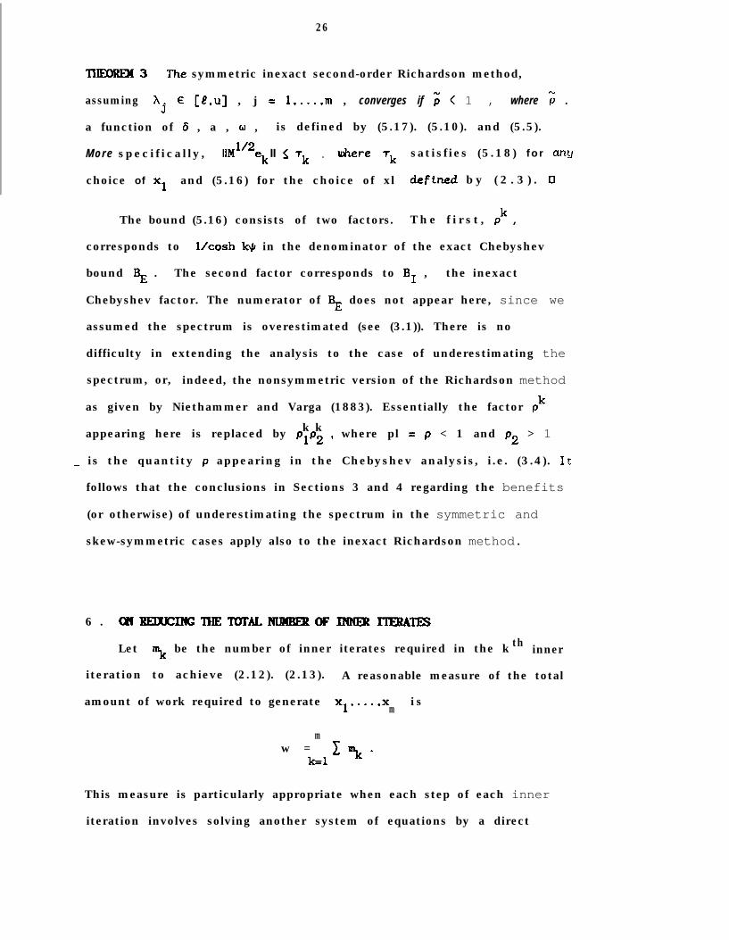
THUXEX3 The symmetric inexact second-order Richardson method,

assuming Aj E [e,u] , j = l.....m , converges if F < 1 , where c .

a function of 6 , a , w , is defined by (5.17). (5.10). and (5.5).

More specifically, llM1’2ek II < Tk . d-me Tk satisfies (5.18) for any

choice of x1 and (5.16) for the choice of xl deftned b y ( 2 . 3 ) . 0

26

I The bound (5.16) consists of two factors. The f i r s t , pk ,

corresponds to l/cash k+ in the denominator of the exact Chebyshev

bound .BE The second factor corresponds to BI , the inexact

Chebyshev factor. The numerator of BB does not appear here, since we

assumed the spectrum is overestimated (see (3.1)). There is no

difficulty in extending the analysis to the case of underestimating the

spectrum, or, indeed, the nonsymmetric version of the Richardson method

as given by Niethammer and Varga (1883). Essentially the factor pk

k kappearing here is replaced by plp2 , where pl = p < 1 and p2 > 1

_ is the quantity p appearing in the Chebyshev analysis, i.e. (3.4). It

follows that the conclusions in Sections 3 and 4 regarding the benefits

(or otherwise) of underestimating the spectrum in the symmetric and

skew-symmetric cases apply also to the inexact Richardson method.

6 . ONREIXXNG’IHE‘IWI’ALNUMBEROFINNERIlERA~

Let mk be the number of inner iterates required in the k th inner

iteration to achieve (2.12). (2.13). A reasonable measure of the total

amount of work required to generate xl,...,x ism

mw = 1 “k.

k=l

This measure is particularly appropriate when each step of each inner

iteration involves solving another system of equations by a direct

27 /

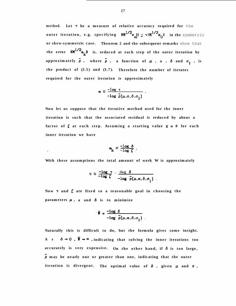
method. Let 7 be a measure of relative accuracy required for the

outer iteration, e.g. specifying llM1’2e II < 711M1’2e IIm - 0 in the symmetric

or skew-symmetric case. Theorem 2 and the subsequent remarks show that

the error llM1’2ekll is. reduced at each step of the outer iteration by

approximately i; , where i , a function of p , a , 6 and aI , is

the product of (3.5) and (3.7). Therefore the number of iterates

required for the outer iteration is approximately

m z -1% 7.

-log P(Cl.a.Lul)

Now let us suppose that the iterative method used for the inner

iteration is such that the associated residual is reduced by about a

factor of 5 at each step. Assuming a starting value z = 0 for each

inner iteration we have

With these assumptions the total amount of work W is approximately

W z -log 7 . -log 6-lo!3 5

-lo g & .wd.ul) l

Now 7 and 5 are fixed so a reasonable goal in choosing the

parameters # , a and 6 is to minimize

-ii = -log 6

-lo i & f.a .6.a l) l

Naturally this is difficult to do, but the formula gives some insight.

A s 6+0, ~-)QD, indicating that solving the inner iterations too

accurately is very expensive. On the other hand, if 6 is too large,

s may be nearly one or greater than one, indicating that the outer

iteration is divergent. The optimal value of & , given p and a ,

28

is somewhere between these extremes. We have already.explained that t.~

plays an important role, which varies with 6 , in the size of c .

Choosing optimal parameters is clearly complicated. However,

substantial insight can be obtained from numerical experiments.

Fortunately, once an adequate choice of parameters has been determined

for a particular problem, whole classes of related problems can usually

be solved efficiently with the same parameter values.

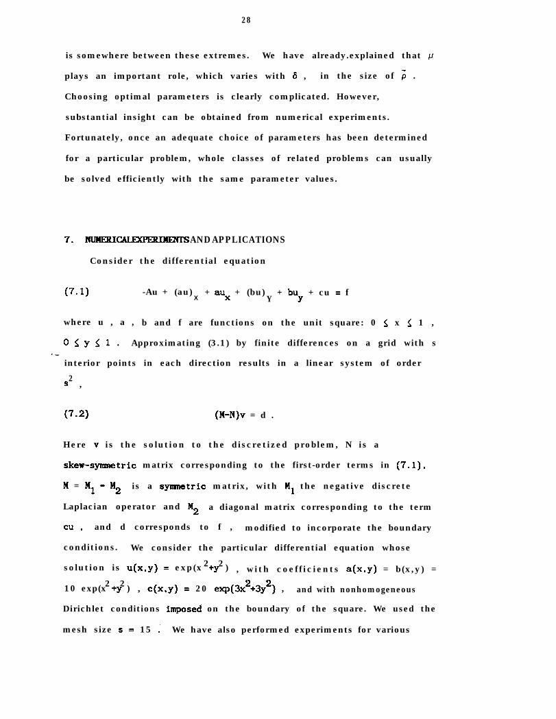
7, NUHERICAL IXPEXIHEKIS AND APPLICATIONS

Consider the differential equation

V-1) -Au + (au) X + aux + (bu)Y

+ buy + cu = f

where u , a , b and f are functions on the unit square: 0 2 x < 1 ,

OIYW. Approximating (3.1) by finite differences on a grid with s.-

interior points in each direction results in a linear system of order

2s ,

(7=2) (M-N)v = d .

Here v is the solution to the discretized problem, N is a

skew-smtric matrix corresponding to the first-order terms in (7.1),

M = Ml - M2 is a synnnetric matrix, with Ml the negative discrete

Laplacian operator and M2 a diagonal matrix corresponding to the term

cu 9 and d corresponds to f , modified to incorporate the boundary

conditions. We consider the particular differential equation whose

2 2solution is u(x.y) = exp(x +y ) , with coefficients a(x,y) = b(x,y) =2 210 exp(x +y ) , c(x,y) = 20 exp(3x2+3y2) , and with nonhomogeneous

Dirichlet conditions imposed on the boundary of the square. We used the

mesh size s = 15 i We have also performed experiments for various

29

other problems. The one reported here was chosen so that both the outer

and the inner systems are moderately difficult to solve. The results

seem fairly typical.

Table III gives the results of solving (7.2) using the

skew-symmetric version of the inexact Chebyshev method with various

choices of ~1 and 6 . (Recall that a = 1.) The initial value x0

was set to zero, and the termination condition for the outer iteration

was llrmll s lO+ . Each inner iteration was carried out using a

(preconditioned) conjugate gradient method, starting with the zero

vector, so that (2.12). (2.13) hold. The symmetric splitting M = Ml -

M2 was exploited so that each step of each inner iteration used a fast

direct method to solve a system of the form Ml; = F , i.e. the Poisson

equation. The entries in the table are of the form “m/w” , i.e. they

report the number of outer iterates and the total number of inner

iterates. .

In addition to the Chebyshev results, Table III gives results for

solving (7.2) using a preconditioned skew-symmetric conjugate gradient

method (see Concus and Golub (1976) and Widlund (1978)). The inner

iterations were carried out exactly as described above, being terminated

by (2.12). (2.13). The results are reported in the column headed CG.

The conjugate gradient method was also run with the inner iterations

carried out to full precision, in order to obtain o1 from the

resulting tridiagonal Lanczos matrix. This run, made solely to compute

la, I . is not included in the table’. It determined that lu,l = 2.19 .

30

TABLE III

6 cc CHEBYSHEV

1/J-+:

10.0 3.0 2.1* 2.0 1.5 1.0 .OOl

0.01 39/274 t 60/401 45/294 76/559 D D D

0.1 461204 1991804 61/249 46/203 461202 D D D

0.5 % 276/603 851194 651149 63/141 188/422 D D

0.9 % % 2991299 2191219 206/206 169/169 132/132 D

Reports # outer iterations/# inner iterations.

Notes: * The value of u1 is 2.101 .

t Number of inner iterates exceeded 1000.

% Number of outer iterates exceeded 500.

D Outer iteration’ diverges.

A careful inspection of Table III reveals a number of interesting

features :

1. Consider the column I~-‘I = la, I = 2.1 . The number of outer

interates increases as d increases, as expected. The total

number of inner iterates, however, reaches a minimum at about

6 = 0.5 . Clearly, a small value of & is inefficient: also, if

d is close to one, only one step is taken in each inner iteration,

which is overall less effective than using d = 0.5 .

2. Consider the Chebyshev results as p varies. For 6 = 0.01 ,

there is a rapid deterioration as 1~1 grows greater than 10;’ I .

For larger 6 , the deterioration is not as rapid and for large

c

6

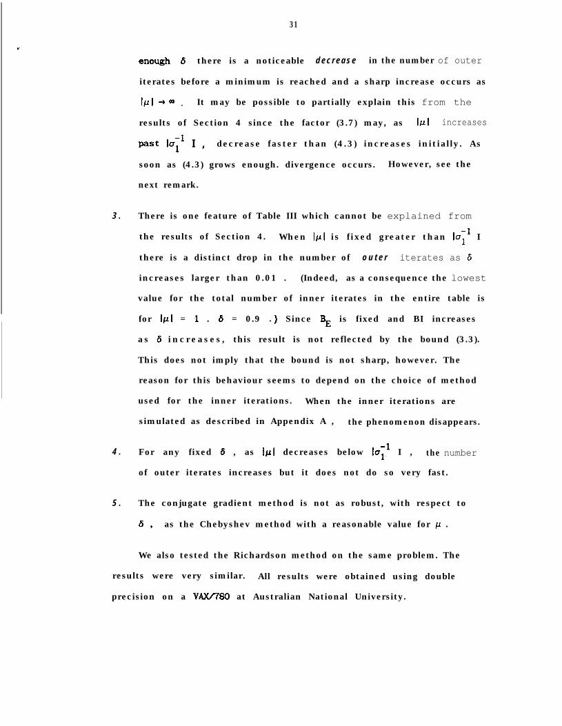
31

there is a noticeable d e c r e a s e in the number of outer

iterates before a minimum is reached and a sharp increase occurs as

lpl *a0 . It may be possible to partially explain this from the

results of Section 4 since the factor (3.7) may, as Id increases

past lu;l I , decrease faster than (4.3) increases initially. As

soon as (4.3) grows enough. divergence occurs. However, see the

next remark.

3 . There is one feature of Table III which cannot be explained from

the results of Section 4. When lpl is fixed greater than luyl I

there is a distinct drop in the number of o u t e r iterates as 6

increases larger than 0.01 . (Indeed, as a consequence the lowest

value for the total number of inner iterates in the entire table is

for IpI = l . 6 = 0.9 .) Since BR is fixed and BI increases

as 6 increases, this result is not reflected by the bound (3.3).

This does not imply that the bound is not sharp, however. The

reason for this behaviour seems to depend on the choice of method

used for the inner iterations. When the inner iterations are

simulated as described in Appendix A , the phenomenon disappears.

4 . For any fixed 6 , as IpI decreases below 1~;’ I , the number

of outer iterates increases but it does not do so very fast.

5 . The conjugate gradient method is not as robust, with respect to

6 s as the Chebyshev method with a reasonable value for p .

We also tested the Richardson method on the same problem. The

results were very similar. All results were obtained using double

precision on a VAX/780 at Australian National University.

32

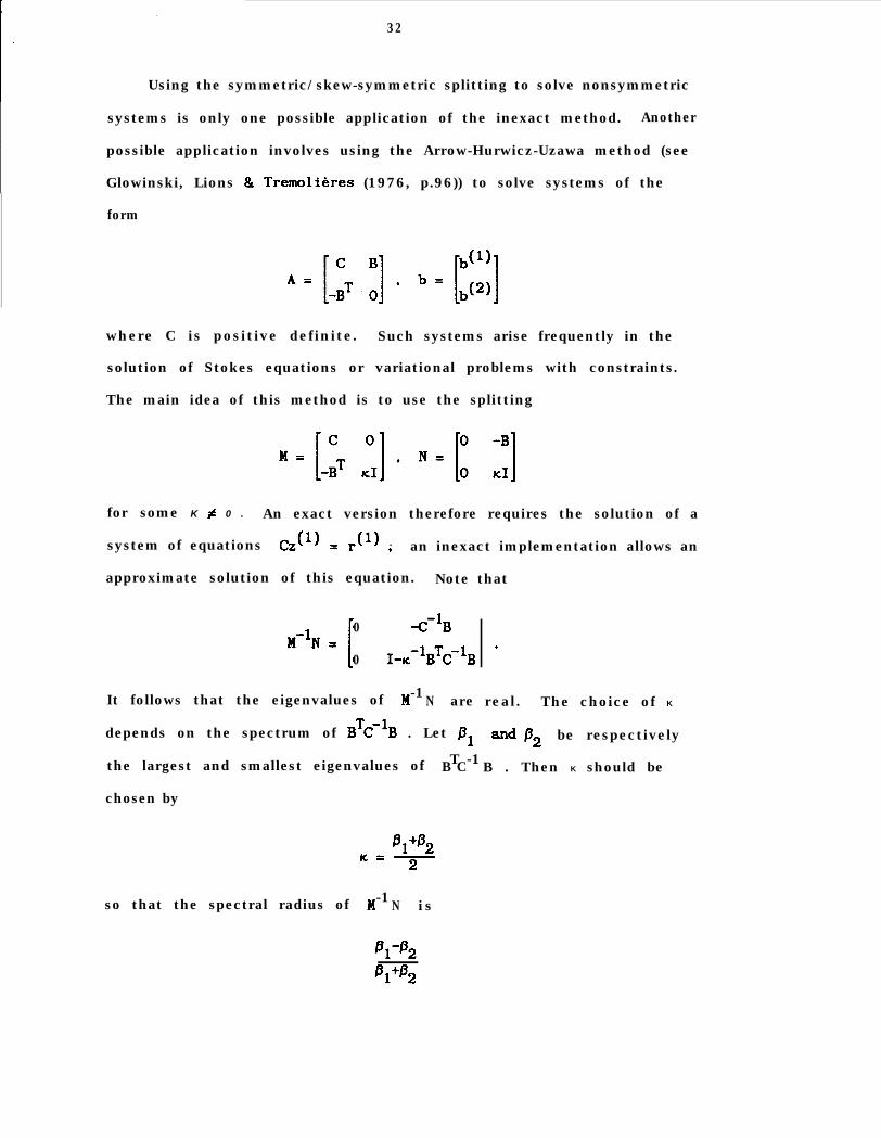
Using the symmetric/skew-symmetric splitting to solve nonsymmetric

systems is only one possible application of the inexact method. Another

possible application involves using the Arrow-Hurwicz-Uzawa method (see

Glowinski, Lions & Tremolieres (1976, p.96)) to solve systems of the

form

where C is positive definite. Such systems arise frequently in the

solution of Stokes equations or variational problems with constraints.

The main idea of this method is to use the splitting

for some K # 0 . An exact version therefore requires the solution of a

system of equations Cz(l) = r (l) l

* an inexact implementation allows an

approximate solution of this equation. Note that

M-$4 =01 &B

0 I-K”B~C-‘B

It follows that the eigenvalues of M-1N are

depends on the spectrum of BTC-‘B . Let /3,

.

real. The choice of K

at-d P2 be respectively

the largest and smallest eigenvalues of T -1B C B . Then K should be

chosen by

so that the spectral radius of -1M N is

VP2

pl+B2

.33

a n d a = 1 in (2.7). Other possible applications of the inexact

iteration include domain decomposftion. * .

.

8. a ⌧va mIms l

We have given a convergence analysis for the inexact Chebyshev and

Richardson methods. We showed that !n the case of the symmetric

iteration, underestimating the eigenvalues speeds up a very inexact

iteration if the spectral radius is large. This is not generally true

in the case of the-skew-symmetric iteration. We have presented

experimental results which indicate that the Ghebyshev & Richardson

methods, with reasonable parameter choices, are less sensitive than the

conjugate gradient method to the degree of inexactness of the iteration.

Finally we note that as parallel computing increases in importance. the

Chebyshev and Richardson methods become more attractive than the

conjugate gradient method since they do not require inner products and

are therefore fully parallelizable.

APPENDIXA

So that others may reproduce the experiments, we give details of

the randomly generated problem discussed in Section 3. We define N to

be a symmetric matrix with a zero diagonal. We used the NAG library

random number generator, initializing it by calling GOSCBF with seed

value 3.0. Subsequently we called GOSGAF to obtain, in order, N1 2 ,9

34

62,1.“. l The values 6k,i were used to obtain qk satisfying

(2.12). (2.13) by ‘.

211rkll(qk)i = ~ ,bk”i ]

-’ l5.‘.

The authors would like to thank Max Dryja and Olof Widlund for

stimulating them to complete this, work. The second author would also

like to thank his hosts at Australian National University for their warm

hosp i ta l i ty . .