Embed Size (px)
Citation preview
THE CONSEQUENCES OF CONSEQUENTIALIST CRITERIA
Nicholas O. Stephanopoulos*
The two most significant approaches to redistricting to emerge in the last generation are
both consequentialist. That is, they both urge authorities to design—and courts to evaluate—
district plans on the basis of the plans’ likely electoral consequences. According to the partisan
fairness approach, plans should treat the major parties symmetrically in terms of the conversion
of votes to seats. According to the competitiveness approach, districts should be as electorally
competitive as is feasible.
Unnoticed by the literature, a substantial number of jurisdictions, in both America and
Australia, have heeded these calls from the academy. In sum, consequentialist criteria have
been used to shape the district plans for close to three hundred elections over the last four
decades. In this paper, I provide an initial assessment of the record of these criteria. The
record, for the most part, is mediocre. Controlling for other relevant factors, partisan fairness
requirements have not made district plans more symmetric in their treatment of the major
parties. Nor have competitiveness requirements made elections more competitive. The likely
explanations are the poor drafting, low prioritization, and need for unrealistically accurate
electoral forecasts of most consequentialist criteria.
However, other common proposals for redistricting reform—in particular, the use of
neutral institutions such as commissions—have performed much better. Elections in Australia,
all of which rely on commissions, are much fairer and more competitive than their American
counterparts. In the United States, commission usage increases both partisan fairness in state
legislative elections and competitiveness in congressional elections, even controlling for an
array of other variables. Ironically, it seems that consequentialist criteria cannot achieve their
own desired consequences—but that non-consequentialist approaches can.
* Assistant Professor of Law, University of Chicago Law School. I am grateful to Christopher Elmendorf,
William Hubbard, Michael McDonald, Eric McGhee, and David Schleicher for their helpful comments. My thanks
also to the workshop participants at the George Washington University Law School, Melbourne Law School, and
Griffith Law School, where I presented earlier versions of the paper.

1 Consequentialist Criteria
TABLE OF CONTENTS
INTRODUCTION .................................................................................................................................1
I. CONSEQUENTIALIST CRITERIA IN THEORY ..................................................................................4
A. Partisan Fairness ..................................................................................................................4
B. Competitiveness ...................................................................................................................6
II. CONSEQUENTIALIST CRITERIA IN PRACTICE ...............................................................................9
A. Methodology ........................................................................................................................9
B. Partisan Fairness ................................................................................................................14
1. South Australia.............................................................................................................14
2. U.S. House of Representatives.....................................................................................17
3. U.S. State Legislatures .................................................................................................19
C. Competitiveness .................................................................................................................21
1. U.S. House of Representatives.....................................................................................21
2. U.S. State Legislatures .................................................................................................23
III. IMPLICATIONS ...........................................................................................................................25
A. Consequentialist Approaches .............................................................................................26
B. Other Approaches ..............................................................................................................30
CONCLUSION ...................................................................................................................................34
APPENDIX .......................................................................................................................................35
INTRODUCTION
The two most significant approaches to redistricting to emerge in the last generation are
both consequentialist. That is, they both urge authorities to design—and courts to evaluate—
district plans on the basis of the plans’ likely electoral consequences. The partisan fairness
approach, associated primarily with political scientists such as Bernard Grofman and Gary King,
argues that plans should treat the major political parties symmetrically. Each party should be
equally able to convert its support from voters into legislative seats. Deviations from symmetry
should be avoided by line-drawers and relied on by courts to invalidate biased plans.
The competitiveness approach, linked to law professors such as Samuel Issacharoff and
Richard Pildes, contends that districts should be as electorally competitive as is feasible.
Competition is the lifeblood of democracy because it makes representatives accountable to voters
and results in a legislature that is responsive to changes in the electorate’s sentiments. It should
therefore be prioritized over all other considerations when the time comes to reshape districts. It
should also be invoked by courts to strike down especially uncompetitive plans.
Almost unnoticed by the literature, a number of jurisdictions, both in America and
abroad, have heeded these calls from the academy and adopted consequentialist redistricting
criteria. With respect to partisan fairness, South Australia enacted a law in 1991 requiring
districts to be drawn so that if a party wins a majority of the popular vote, it will also win a
majority of seats in the legislature. Delaware and Hawaii have longstanding provisions barring
district plans that “unduly favor” a party. And legislatures, commissions, and courts in thirteen
other U.S. states have taken partisan fairness into account on at least one occasion since 1966.

Consequentialist Criteria 2
With respect to competitiveness, laws in Arizona, Washington, and Wisconsin include (or
formerly included) it as a mandatory line-drawing criterion. Legislatures, commissions, and
courts in six other U.S. states also have sought voluntarily to craft competitive districts at least
once in the modern redistricting era. In total, partisan fairness and competitiveness have been
used to design the district plans for close to three hundred South Australian, congressional, and
state legislative elections over the last four decades. This is a far larger universe of cases than
previously has been realized.
In this paper, I investigate the consequences of these consequentialist criteria. I
investigate, in other words, whether plans enacted pursuant to a partisan fairness requirement
actually treat the major parties more symmetrically, and whether plans enacted pursuant to a
competitiveness criterion in fact result in more competitive elections. To carry out this
investigation, I compiled the results of all federal and state elections held in Australia since 1990,
as well as South Australian state election results since 1950. I also compiled all American
congressional and state legislative election results since 1966, when the one-person, one-vote
rule was first implemented nationwide.
Once I assembled this data, I calculated several measures of partisan fairness and
competitiveness for each jurisdiction in each election year. My measures of partisan fairness
were (1) partisan bias, i.e., the divergence in the share of seats that each party would win given
the same share of the statewide vote; and (2) the efficiency differential, i.e., the gap between the
parties’ respective “wasted” votes. My measures of competitiveness were (1) average margin of
victory, i.e., the average difference in vote shares between the winning and losing candidates; (2)
share of competitive seats, i.e., the proportion of races decided by less than a twenty-point
margin; and (3) electoral responsiveness, i.e., the rate at which a party gains or loses seats given
changes in its overall vote share. All of these metrics are widely used by political scientists.
At first glance, my results seem promising for advocates of consequentialist criteria.
South Australia has enjoyed lower levels of partisan bias and smaller efficiency differentials than
other Australian states since adopting its partisan fairness rule in 1991. So too have U.S. states
that have employed similar requirements, in both congressional and state legislative elections. In
terms of competitiveness as well, average margins of victory are smaller, shares of competitive
seats are larger, and rates of electoral responsiveness are higher in U.S. states that explicitly have
tried to draw competitive districts. These effects are particularly pronounced at the state
legislative level.
Unfortunately, many of these results become less impressive when the data is subjected
to more sophisticated analysis. For example, South Australia’s partisan bias levels and
efficiency differentials are not lower than those that it featured prior to adopting its partisan
fairness requirement. Nor does South Australia’s current advantage over its fellow states remain
statistically significant when controls are added for factors such as the year, the level of election,
and the number of districts. Similarly, statistical significance disappears in most (though not all)
U.S. models when controls are added for the redistricting institution, other line-drawing criteria,
whether the state government was unified or divided, and other relevant variables. One
exception is that partisan fairness requirements continue to reduce the efficiency differential in

3 Consequentialist Criteria
congressional elections. A more important exception is that competitiveness criteria continue to
decrease the average margin of victory and increase the share of competitive seats and the level
of electoral responsiveness in state legislative elections.
What are we to make of this picture? The most obvious lesson is that consequentialist
criteria have not, to date, delivered their promised consequences, at least not in their promised
magnitude. Levels of partisan fairness and competitiveness simply have not risen very much
even when jurisdictions have enacted requirements specifically aimed at raising them. This may
be because the provisions were drafted poorly—for instance, what does it mean to “unduly
favor” a party? Or it may be because the provisions were not prioritized very highly, but rather
were considered only after several other criteria were applied first. Or, most discouragingly, it
may be because redistricting authorities are largely incapable of predicting future election
results. Consequentialist criteria may not work because electoral consequences cannot be
forecast accurately enough.
A second implication is that, to the extent that consequentialist criteria do work, they do
so most clearly in the case of competitiveness requirements applied to state legislative elections.
This is the one domain in which the use of consequentialist criteria remained significant even
after adding the full panoply of controls. It is possible that competitiveness is easier for line-
drawers to predict than partisan fairness. The various measures of competitiveness are simpler to
compute than their partisan fairness counterparts, and they are linked as well to foreseeable
factors such as the presence of incumbents. It is also possible that state legislative elections are a
more favorable setting for consequentialist criteria than congressional elections. Their lower
stakes may make district-drafters more willing to pursue goals other than partisan or bipartisan
advantage. And their larger numbers of districts may provide drafters with more cartographic
flexibility while also improving the accuracy of the various metrics (which are more volatile
when the number of districts is small).
A final point is that common proposals for redistricting reform other than the adoption of
consequentialist criteria seem to work quite well. South Australia’s partisan bias levels and
efficiency differentials did not drop when it adopted its partisan fairness requirement, but they
plummeted after it instituted an independent commission in 1975. Australian elections as a
whole, all of which rely on commissions, are much more symmetric in their treatment of the
major parties, and much more competitive, than their American analogues. In the United States,
commission usage increases partisan fairness in state legislative elections and boosts
competitiveness in congressional elections, even controlling for an array of other factors. The
use of familiar line-drawing criteria such as respect for political subdivisions also has a strong
pro-competitive effect at both the state legislative and congressional levels. Accordingly, the
relative ineffectiveness of consequentialist criteria is no cause for despair. Less exotic reform
options can achieve many of the same consequentialist goals, while also realizing a number of
other desirable values.
The paper proceeds as follows. Part I introduces the partisan fairness and
competitiveness approaches and discusses their normative foundations. Part II, the paper’s
analytical core, examines empirically the consequences of consequentialist criteria. Finally, Part
III explores some of the legal and policy implications of the previous section’s findings.

Consequentialist Criteria 4
I. CONSEQUENTIALIST CRITERIA IN THEORY
Two approaches to redistricting have dominated the academic debate over the last
generation: the partisan fairness approach, advocating that district plans treat the major parties
symmetrically, and the competitiveness approach, advising that districts be made as competitive
as is feasible.1 Both of these approaches are consequentialist because they urge that districts be
drawn on the basis of their likely electoral consequences. In this Part, I summarize the two
approaches, present the normative theories that underlie them, and set forth some of their
respective strengths and weaknesses.
A. Partisan Fairness
The partisan fairness approach, which is “virtually a consensus position of the [political
science] community,”2 asserts that district plans should not vary in their treatment of the major
parties. Each party should be equally able to convert its support among the electorate into seats
in the legislature. If one party receives a certain share of seats for a certain share of votes, then
the other party should receive the same seat share for this vote share. Importantly, partisan
fairness is not the same thing as proportional representation. It is perfectly permissible for one
party to receive, say, 65% of seats for 55% of votes, as long as the other party also would receive
65% of seats were it to muster 55% of votes.3
A particular kind of equality principle motivates the partisan fairness approach. It is a
principle that applies to political parties, not to other organized groups or individuals. It is also a
principle whose touchstone is the conversion of statewide votes to statewide seats, not ballot
access or financial resources or efficacy in campaigning. Parties are the key entities that are
understood to be affected by redistricting, and vote-seat conversion is the key concept that is
understood to be at issue. As Grofman and King put it, the “idea is that candidates of each
political party should have equal opportunity in translating voter support into the division of
legislative seats between the parties.”4
Although its reasoning is notoriously difficult to grasp, the Supreme Court decision that
first recognized a cause of action for gerrymandering, Davis v. Bandemer,5 relied in part on this
partisan equality principle. The claim whose validity the Court acknowledged was that “each
political group in a State should have the same chance to elect representatives of its choice as
1 See Adam B. Cox, Partisan Gerrymandering and Disaggregated Redistricting, 2004 SUP. CT. REV. 409,
419-27 (2004) (presenting as two “conventional accounts” of redistricting the “partisan bias account” and the
“anticompetition account”). 2 Bernard Grofman & Gary King, The Future of Partisan Symmetry as a Judicial Test for Partisan
Gerrymandering After LULAC v. Perry, 6 ELECTION L.J. 2, 6 (2007); see also Andrew Gelman & Gary King,
Enhancing Democracy Through Legislative Redistricting, 88 AM. POL. SCI. REV. 541, 554 (1994) (“The vast
majority of American political scientists have adopted the normative position that healthy representative
democracies have low levels of partisan bias . . . .”). 3 See Grofman & King, supra note 2, at 8.
4 Id.
5 478 U.S. 109 (1986).

5 Consequentialist Criteria
any other political group.”6 Partisan fairness played almost no role in the Court’s 2004
gerrymandering decision, Vieth v. Jubelirer,7 but it resurfaced in the 2006 case of League of
United Latin American Citizens (LULAC) v. Perry.8 In his opinion for the Court, Justice
Kennedy declined to endorse the partisan fairness approach, but he did note “its utility in
redistricting planning and litigation.”9 Other Justices were not so circumspect. Justice Stevens
observed that the approach is “widely accepted by scholars,”10
praised it as a “helpful (though
certainly not talismanic) tool,”11
and analyzed Texas’s district plan in terms of the symmetry of
its treatment of the major parties.12
Similarly, Justice Souter cited the “utility of a criterion of
symmetry as a test” and remarked that “[i]nterest in exploring this notion is evident.”13
The appeal of the partisan fairness approach is that it captures the primary harm that is
caused by gerrymandering. A district plan is typically considered a gerrymander in favor of a
party precisely because the plan enables the party to convert votes to seats more efficiently than
its opponent. A party is typically deemed the victim of gerrymandering precisely because its
popular support does not translate into legislative strength with the same ease as its adversary’s.
The partisan fairness approach also is attractive because it focuses on a jurisdiction as a whole,
not on the shape or composition of individual districts. There are many innocent explanations
for districts’ appearance and makeup, so it is preferable to concentrate on the overall rather than
the local picture. The approach’s final advantage is that it lends itself easily to quantification.
As I discuss in Part II, metrics such as partisan bias and the efficiency differential reveal how fair
or unfair a plan is to the major parties.
On the other hand, a problem with the partisan fairness approach is that unequal
treatment of the parties is often the result of a jurisdiction’s underlying political geography, not a
deliberate attempt to gerrymander. For example, if Democrats tend to live in urban areas that are
overwhelmingly Democratic, while Republicans live mostly in suburbs and exurbs that are more
evenly divided, then any plan that respects subdivision boundaries will be biased in a Republican
direction.14
Unequal partisan effect is not a sure sign of illicit partisan intent. Another issue with
the approach is that it overlooks all values implicated by redistricting other than the treatment of
the parties in terms of vote-seat conversion. To name a few, voter participation, minority
influence, and the quality of representation all are influenced by how districts are drawn, but all
are paid no heed by the approach. A final, more technical concern is that the usual metrics of
partisan fairness are somewhat unreliable. Partisan bias and efficiency differential scores
6 Id. at 124.
7 541 U.S. 267 (2004).
8 548 U.S. 399 (2006).
9 Id. at 420.
10 Id. at 467 (Stevens, J., concurring in part and dissenting in part).
11 Id. at 468 n.9.
12 See id. at 467.
13 Id. at 483 (Souter, J., concurring in part and dissenting in part).
14 See Jowei Chen & Jonathan Rodden, Using Legislative Districting Simulations to Measure Electoral Bias
in Legislatures 30 (July 15, 2010) (finding that district plans of most U.S. states containing major cities are biased in
Republican direction); Jonathan Rodden, The Geographic Distribution of Political Preferences, 13 ANNUAL REV.
POL. SCI. 321, 332 (2010) (noting that redistricting biases against leftist parties have existed in many countries
“going back to the turn of the century”).

Consequentialist Criteria 6
fluctuate from election to election, especially when a jurisdiction has few districts, and the
former measure relies upon the problematic assumption of uniform partisan swing.15
Despite these difficulties, at least sixteen jurisdictions—South Australia and fifteen U.S.
states—have used partisan fairness as a criterion to design the district plans for at least 193
elections. Whether the criterion has actually achieved its aim of making plans more symmetric
in their treatment of the major parties has never previously been investigated.16
It is to this
important question that I turn in Part II.
B. Competitiveness
The other consequentialist approach to redistricting to emerge in recent years prizes
competitiveness rather than partisan fairness. It contends that districts in a jurisdiction should be
drawn so that they are as competitive as is reasonably possible. Not all districts should be made
competitive, because some geographic regions are highly uncompetitive and their integrity
usually should be respected.17
But what is clearly unacceptable is the deliberate suppression of
the competition that would arise in a jurisdiction if district lines were drawn pursuant to
conventional redistricting criteria. As Issacharoff writes, “The question is . . . whether districts
may be rigged so as to diminish or eliminate competition that would otherwise emerge from
redistricting not controlled by incumbent partisan power.”18
The normative reason to prioritize competitiveness so highly is that it promotes the
realization of several important democratic values. First, individual politicians are more
accountable to voters when districts are competitive. Closer races make it easier for voters to
oust from office politicians of whose records they disapprove.19
Second, competitiveness
15
The uniform swing assumption stipulates that parties’ district-specific vote shares change (or “swing”) by
the same margin as their statewide vote shares. For example, if the Democrats received 45% of the vote in a state,
and a researcher wanted to know how many seats they would have won if they had received 50%, the researcher
would simply add 5% to the actual Democratic vote share in each district. See Nicholas O. Stephanopoulos, Spatial
Diversity, 125 HARV. L. REV. 1903, 1963-64 (2012). The assumption usually generates accurate seat share
estimates, but is still considered “neither theoretically nor empirically satisfying” by certain political scientists.
Simon Jackman, Measuring Electoral Bias: Australia, 1949–93, 24 BRIT. J. POL. SCI. 319, 335 (1994). 16
To be more precise, this issue has never been investigated with respect to American jurisdictions. Jenni
Newton-Farrelly has written an illuminating series of articles on the South Australian case, finding that the state’s
partisan fairness requirement has generally performed well. See Jenni Newton-Farrelly, From Blindfolds to Naked
Emperors [hereinafter Newton-Farrelly, Blindfolds]; Jenni Newton-Farrelly, From Gerry-Built to Purpose-Built, 45
REPRESENTATION 471 (2009) [hereinafter Newton-Farrelly, Gerry-Built]; Jenni Newton-Farrelly, Wrong Winner
Election Outcomes in South Australia (South Australian Parliament Research Library, Research Paper No. 21, 2010)
[hereinafter Newton-Farrelly, Wrong Winner]. 17
See Samuel Issacharoff & Pamela S. Karlan, Where to Draw the Line?, 153 U. PA. L. REV. 541, 574
(2004) (“Nor is our claim that an electoral system requires every district to be competitive. There will always be
Berkeley and Orange County . . . .”); Richard H. Pildes, The Constitution and Political Competition, 30 NOVA L.
REV. 253, 261 (2006) (“To ensure that all elections are competitive is, of course, impossible.”). 18
Samuel Issacharoff, Why Election?, 116 HARV. L. REV. 684, 692 (2002). 19
See Samuel Issacharoff, Gerrymandering and Political Cartels, 116 HARV. L. REV. 593, 616 (2002)
(“[A]ccountability is a central feature of democratic legitimacy . . . .”); Michael P. McDonald & John Samples, The
Marketplace of Democracy, in THE MARKETPLACE OF DEMOCRACY 1,5 (Michael P. McDonald & John Samples

7 Consequentialist Criteria
increases the responsiveness of the electoral system as a whole. Shifts in the electorate’s views
have a greater impact on the composition of the legislature when more districts are competitive
(and thus can swing from one party to another).20
Lastly, competitiveness is linked to voter
participation. Voters learn more about candidates and are more likely to turn out at the polls
when there is some uncertainty about races’ outcomes.21
Unlike the partisan fairness approach, the competitiveness approach has never been
endorsed by the Supreme Court. In Vieth, Justice Souter did refer to the “analogy to antitrust,” a
domain in which anti-competitive practices are prohibited, as “an intriguing one that may prove
fruitful.”22
However, he then added that he did “not embrace [the analogy] at this point out of
caution about a wholesale conceptual transfer from economics to politics.”23
Similarly, Justice
Stevens observed in LULAC that uncompetitive races can lead to lower voter turnout and higher
legislative polarization.24
But his opinion focused on partisan intent rather than lack of
competition, and he did not suggest that a plan could be invalidated for the latter reason.25
And
in the 1973 decision of Gaffney v. Cummings, the Court actually approved a Connecticut plan
that created 130 safe state house districts and only 20 competitive districts.26
The Court was
untroubled by the plan’s reduction of competition in order to produce a “proportionate number of
Democratic and Republican legislative seats.”27
The appeal of the competitiveness approach stems from the democratic values that it aims
to realize. Accountability, responsiveness, and participation all are widely seen as key elements
of a vibrant democracy—and all are improved by increases in district-level competitiveness.28
The approach is also attractive because it captures another harm that is sometimes thought to be
caused by gerrymandering: the creation of safe districts that insulate politicians (particularly
incumbents) from any real risk of losing their seats. This is not the primary harm that is
associated with gerrymandering (that would be partisan unfairness), but it is an important
consideration nonetheless.29
The approach’s final advantage is that it too lends itself to
eds., 2006) (“[D]emocratic theorists value electoral competition as a way to ensure that representatives are
accountable to voters.”). 20
See Gelman & King, supra note 2, at 544 (“Scholars of American politics almost uniformly take the
normative position that higher values of responsiveness indicate a healthier democracy.”); Samuel Issacharoff &
Richard H. Pildes, Politics as Markets, 50 STAN. L. REV. 643, 646 (1998) (“Only through an appropriately
competitive partisan environment can . . . policy outcomes of the political process be responsive to the interests and
views of citizens.”). 21
See Pildes, supra note 17, at 260 (“[I]t is well documented that competitive elections . . . increase voter
turnout . . . .”). 22
Vieth v. Jubelirer, 541 U.S. 267, 350 n.5 (2004) (Souter, J., dissenting). 23
Id. 24
See LULAC v. Perry, 548 U.S. 399, 471 n.10 (2006) (Stevens, J., concurring in part and dissenting in
part). 25
See id. 26
412 U.S. 735, 738 n.4 (1973). 27
Id. at 738; see also Issacharoff, supra note 19, at 612-17 (criticizing Gaffney on this basis). 28
See Nathaniel Persily, The Place of Competition in American Election Law, in THE MARKETPLACE OF
DEMOCRACY, supra note 19, at 171, 173 (“[P]olitical competition is primarily a means to other ends: namely, greater
accountability, responsiveness . . . and participation in government.”). 29
See LULAC, 548 U.S. at 471 n.10 (Stevens, J., concurring in part and dissenting in part) (discussing the
ways in which “[s]afe seats may harm the democratic process”).

Consequentialist Criteria 8
quantification. Metrics such as average margin of victory, share of competitive seats, and
electoral responsiveness indicate both how competitive individual districts are and how
responsive a jurisdiction’s electoral system is as a whole.
Conversely, a problem with the competitiveness approach is that it ignores the concept—
the unequal treatment of the parties in terms of vote-seat conversion—that lies at the heart of the
usual definition of gerrymandering.30
That certain districts are uncompetitive, or that a plan in
its entirety is non-responsive, is certainly very interesting, but it is not typically thought to be
evidence that a gerrymander has been enacted. Another issue with the approach is that
competitiveness is not in fact an unalloyed good. Closer races result in more dissatisfied voters
who would have preferred a different outcome,31
and very high responsiveness means that small
changes in voter sentiment produce very large changes in legislative composition.32
Finally, like
the partisan fairness approach, the competitiveness approach neglects values such as minority
influence and the quality of representation, and its quantitative metrics are relatively volatile.33
These difficulties have not stopped a substantial number of jurisdictions—nine U.S.
states in 103 elections—from using competitiveness as a criterion to design their district plans.
Whether the criterion has actually accomplished its goal of making elections more competitive is
a question that only recently has begun to be considered. One study found that Arizona’s
adoption of a competitiveness criterion in 2000 did not make its elections any more
competitive.34
Another study determined that “political” requirements, including both
competitiveness criteria and rules on incumbent protection, reduced the vote shares received by
incumbents nationwide.35
No work to date has examined the consequences of only
competitiveness criteria in all of the jurisdictions that have employed them. The paper’s next
Part offers precisely such an examination.
30
See Vieth, 541 U.S. at 271 n.1 (plurality opinion) (“The term ‘political gerrymander’ has been defined as
‘[t]he practice of dividing a geographical area into electoral districts . . . to give one political party an unfair
advantage by diluting the opposition's voting strength.’”). 31
See Thomas L. Brunell, Rethinking Redistricting, 39 PS: POL. SCI. & POL. 77, 77-81 (2006) (arguing
against competitive districts for this reason). 32
See Nathaniel Persily, In Defense of Foxes Guarding Henhouses, 116 HARV. L. REV. 649, 668 (2002)
(noting that if there are too many competitive districts in a jurisdiction, then “the slightest shift in voter preferences
would lead to a landslide victory for one of the parties”). 33
See supra text accompanying note 15. 34
See Barbara Norrander & Jay Wendland, Redistricting in Arizona, in REAPPORTIONMENT AND
REDISTRICTING IN THE WEST 177, 191 (Gary Moncrief ed., 2011). 35
See Richard Forgette & Glenn Platt, Redistricting Principles and Incumbency Protection in the U.S.
Congress, 24 POL. GEOGRAPHY 934, 939, 946 (2005); see also Richard Forgette et al., Do Redistricting Principles
and Practices Affect U.S. State Legislative Electoral Competition?, 9 STATE POL. & POL’Y Q. 151, 155 (2009)
[hereinafter, Forgette et al., Do Principles?] (referring to states that use competitiveness criteria but only actually
considering states with incumbency protection rules in analysis); Richard Forgette et al., The Un-Principled Politics
of State Legislative and Congressional Redistricting 7 (Sept. 2-5, 2005) [hereinafter Forgette et al., Un-Principled
Politics] (same); cf. Nicholas O. Stephanopoulos, Our Electoral Exceptionalism, 79 U. CHI. L. REV. (forthcoming
2013) (manuscript at 24-25) (summarizing inconclusive literature on implications of redistricting institutions for
competitiveness).
9 Consequentialist Criteria
II. CONSEQUENTIALIST CRITERIA IN PRACTICE
Now that the two consequentialist approaches to redistricting have been introduced, it is
possible to turn to the question that motivates this paper: What are the actual consequences of
consequentialist criteria? Do they in fact achieve their aims of greater partisan fairness and
increased competitiveness? I begin this Part by explaining my methodology, and I then present
the results of my analysis with respect to both partisan fairness (for South Australia, the U.S.
House of Representatives, and American state legislatures) and competitiveness (for the U.S.
House and state legislatures). In a nutshell, my principal finding is that consequentialist criteria
have not been very successful at bringing about their intended consequences, though there is
plenty more to the story.
A. Methodology
To begin with, I compiled the results of all federal and state elections held in Australia
since 1990, as well as South Australian state election results since 1950.36
South Australia
adopted its partisan fairness requirement in 1991,37
so there was little reason to gather
comprehensive data from prior to this date. I also compiled all American congressional and state
legislative election results since 1966,38
the year the one-person, one-vote rule was first enforced
in almost all elections.39
The first consequentialist criteria were not implemented until 1972, but
the climax of the reapportionment revolution seemed like a better starting point for my study
than the unheralded innovations of a handful of states.
Next, I tried to identify all states that have ever employed consequentialist criteria in the
modern era, as well as the years of the elections in which the criteria were used. In some cases,
this task was relatively straightforward. For example, the state laws of Arizona, Delaware,
Hawaii, and Washington currently include partisan fairness or competitiveness requirements, and
36
Federal election results are available at AUSTRALIAN ELECTORAL COMMISSION, DOWNLOAD OFFICIAL
ELECTION STATISTICS, http://www.aec.gov.au/Elections/Federal_Elections/Stats_CDRom.htm (Jan. 24, 2011).
Recent state election results are available at ABC NEWS, ELECTION ARCHIVE, http://www.abc.net.au/elections/
archive/ (last visited Dec. 1, 2012). Jenni Newton-Farrelly shared with me historical South Australian election
results compiled by Colin Hughes, and I am very grateful for her help. I only analyzed Australia’s five largest states
(New South Wales, Queensland, South Australia, Victoria, and Western Australia), and I only used Western
Australia’s 2008 state election because prior to this date it did not abide by the one-person, one-vote rule. 37
See SOUTH AUSTRALIA STATE ELECTORAL OFFICE, SOUTH AUSTRALIAN ELECTORAL BOUNDARY
REDISTRIBUTIONS, 1851-2003, at 4, 7 (2006). 38
Congressional election results are available at U.S. HOUSE OF REPRESENTATIVES, OFFICE OF THE CLERK,
ELECTION INFORMATION, http://clerk.house.gov/member_info/electionInfo/index.aspx (last visited Dec. 1, 2012),
and also, in a more usable format, in a database that Gary Jacobson shared with me. Jacobson’s database contains
presidential election results aggregated by congressional district as well. I conducted all of my congressional
analysis using this data too, but my findings were not as easily interpretable. Not surprisingly, variables pertaining
to congressional races predict congressional results more accurately than aggregated presidential results. For state
legislative election results, I relied entirely on a comprehensive database that Carl Klarner has recently assembled.
The congressional data includes the results of the 2012 elections, while the state legislative data is only available
through 2010. Presidential election results aggregated by state legislative district are not available. 39
See Leroy Hardy et al., Introduction, in REAPPORTIONMENT POLITICS 17, 19 (Leroy Hardy et al. eds.,
1981) (“By 1966, legislatures in 46 of the 50 states had brought their apportionments into compliance with the new
judicial standards of population equality”).

Consequentialist Criteria 10
it was not hard to determine when these requirements were enacted. In many cases, however,
consequentialist criteria were not memorialized in state laws, but rather were invoked on an ad
hoc basis by legislatures, commissions, or courts. I found these cases by searching the relevant
case law, examining state redistricting websites, and consulting historical resources on
redistricting. I cannot be certain that I have located all cases in which consequentialist criteria
were used, but I am reasonably confident that I have discovered the vast majority of them.
Notably, the National Conference of State Legislatures, the best-informed organization about
redistricting around the country, could not identify any cases that I have missed.40
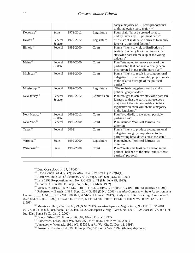
Figures 1 and 2 list the states (and institutions within them) that have employed
consequentialist criteria, the levels and years of the elections in which they did so, and the key
language that they issued. Consequentialist criteria have been used for about twice as many state
legislative elections as congressional elections. They have been used about twice as often in the
last two full redistricting cycles (the 1990s and 2000s) as in the two before them (the 1970s and
1980s). And they have been used about twice as often by courts as by legislatures and
commissions put together. The most common partisan fairness formulations include assertions
that the concept was considered, bans on plans that unduly favor a party, requirements of
approximate seat-vote proportionality, and requirements that whichever party wins a majority of
votes also should win a majority of seats. The most common competitiveness formulations
either state that the concept was taken into account or declare that larger numbers of competitive
districts were created.
FIGURE 1: JURISDICTIONS USING PARTISAN FAIRNESS CRITERIA
Jurisdiction Level Elections Used Institution Key Language
South Australia41
State 1993-2010 Legislature “[I]f candidates of a particular group
attract more than 50 per cent of the popular
vote . . . they will be elected in sufficient
numbers to enable a government to be
formed”
California42
Federal
& state
1974-1980 Court Plans are not “politically unfair” and will
not “produce a manifestly unfair political
result”
Colorado43
Federal 2002-2010 Court “Finally, we check our plan against the test
of general partisan outcome”
Connecticut44
State 1972-1980 Legislature “[W]hichever party carried the state should
40
Importantly, I do not include in my study provisions that bar district plans from being drawn with the
intent to help or harm a party or candidate. California, Florida, Idaho, Iowa, Minnesota, Nebraska, Oregon, and
Washington use such provisions, but they are not consequentialist since they do not aim to produce election results
that are fair to the major parties. It is also possible that redistricting authorities have employed consequentialist
criteria without ever stating in writing that they did so. I doubt there are many such cases but I cannot be sure.
Lastly, the fact that many consequentialist criteria have been used without being formally memorialized actually
improves the accuracy of my empirical analysis. It means that the criteria were not adopted as components of
broader electoral reforms, thus allaying concerns about endogeneity and omitted variables. 41
South Australia Constitution Act 1934 (Cth) s 83 (Austl. S.A.). 42
Legislature v. Reinecke, 516 P.2d 6, 38 (Cal. 1973). 43
Avalos v. Davidson, 2002 WL 1895406, at *8 (Colo. Dist. Ct. Jan. 25, 2002). 44
Cummings v. Meskill, 341 F. Supp. 139, 147 (D. Conn. 1972).
11 Consequentialist Criteria
carry a majority of . . . seats proportional
to the statewide party majority”
Delaware45
State 1972-2012 Legislature Plans shall “[n]ot be created so as to
unduly favor any . . . political party”
Hawaii46
Federal
& state
1972-2012 Legislature “No district shall be so drawn as to unduly
favor a . . . political faction”
Illinois47
Federal 1992-2000 Court Plan is “likely to yield a distribution of
seats across party lines that mirrors the
statewide partisan makeup of the voting
citizenry”
Maine48
Federal
& state
1994-2000 Court Plan “attempted to remove some of the
partisanship that had inadvertently been
incorporated in our preliminary plan”
Michigan49
Federal 1992-2000 Court Plan is “likely to result in a congressional
delegation . . . that is roughly proportionate
to the relative strength of the political
parties.”
Mississippi50
Federal 1992-2000 Legislature “The redistricting plan should avoid a
political gerrymander”
New Jersey51
Federal
& state
1982-2012 Commission Plan “sought to achieve statewide partisan
fairness so that the party that receives a
majority of the total statewide vote in a
legislative election will obtain a majority
in the legislature”
New Mexico52
Federal
& state
2002-2012 Court Plan “avoid[ed], to the extent possible,
partisan bias”
New York53
Federal 1992-2000 Court Plan included “political fairness” as
criterion
Texas54
Federal 2002 Court Plan is “likely to produce a congressional
delegation roughly proportional to the
party voting breakdown across the state”
Virginia55
State 1992-2000 Legislature Plan included “political fairness” as
criterion
Wisconsin56
State 1992-2000 Court Plan “creates the least perturbation in the
political balance of the state” and is “least
partisan” proposal
45
DEL. CODE ANN. tit. 29, § 804(4). 46
HAW. CONST. art. 4, § 6(2); see also HAW. REV. STAT. § 25-2(b)(1). 47
Hastert v. State Bd. of Elections, 777. F. Supp. 634, 659 (N.D. Ill. 1991). 48
In re 1993 Reapportionment, No. SJC-229, at *1 (Me. June 29, 1993). 49
Good v. Austin, 800 F. Supp. 557, 566 (E.D. Mich. 1992). 50
MISS. STANDING JOINT CONG. REDISTRICTING COMM., CRITERIA FOR CONG. REDISTRICTING 3 (1991). 51
Robertson v. Bartels, 148 F. Supp. 2d 443, 459 (D.N.J. 2001); see also Gonzalez v. State Apportionment
Comm’n, ___ A.3d ___, 2012 WL 3889021, at *4-5 (N.J. Super. 2012); Brady v. N.J. Redistricting Comm’n, 622
A.2d 843, 619 (N.J. 1992); DONALD E. STOKES, LEGISLATIVE REDISTRICTING BY THE NEW JERSEY PLAN 7-17
(1993). 52
Maestas v. Hall, 274 P.3d 66, 79 (N.M. 2012); see also Jepsen v. Vigil-Giron, No. D0101 CV 2001
02177, at 9 (1st Jud. Dist. Santa Fe Co. Jan. 24, 2002); Jepsen v. Vigil-Giron, No. D0101 CV 2001 02177, at 5 (1st
Jud. Dist. Santa Fe Co. Jan. 2, 2002). 53
Diaz v. Silver, 978 F. Supp. 96, 102, 104 (E.D.N.Y. 1997). 54
Balderas v. Texas, 2001 WL 36403750, at *3 (E.D. Tex. Nov. 14, 2001). 55
Jamerson v. Womack, 1991 WL 835368, at *1 (Va. Cir. Ct. Dec. 11, 1991). 56
Prosser v. Elections Bd., 793 F. Supp. 859, 871 (W.D. Wis. 1992) (three-judge court).

Consequentialist Criteria 12
FIGURE 2: JURISDICTIONS USING COMPETITIVENESS CRITERIA
Jurisdiction Level Elections Used Institution Key Language
Arizona57
Federal
& state
2002-2012 Commission “To the extent practicable, competitive
districts should be favored . . . .”
California58
Federal
& state
1974-1980 Court Plan will “result in fewer ‘safe seats’ and
more ‘competitive seats’”
Colorado59
Federal
& state
1992-2012 Commission
& court
Plan “considered competitiveness as an
important factor”
Florida60
Federal 1992-2000 Court Plan “considered . . . party
competitiveness”
New Jersey61
State 1982-2012 Commission Plan “ensur[ed] that some seats were
competitive so that the composition of the
Legislature would be responsive to shifts
in votes from one party to the other”
New Mexico62
Federal
& state
2002-2010 Court Plan “promote[s] . . . political
competition”
North Carolina63
Federal 2012 Legislature Plan had as goal “to create more
competitive Congressional districts”
Washington64
Federal
& state
1992-2012 Commission “The commission shall exercise its powers
to . . . encourage electoral competition”
Wisconsin65
State 1984-1990 Legislature Plan gave “due consideration to the need
for . . . competitive legislative districts”
After compiling all the relevant election results and identifying all the relevant cases, the
next stage of my analysis was to calculate measures of partisan fairness and competitiveness for
each jurisdiction in each election year. My first partisan fairness metric was partisan bias, that
is, the divergence in the share of seats that each party would win given the same share of the
statewide vote.66
For example, if Democrats would win 48% of a state’s seats with 50% of the
state’s vote (in which case Republicans would win 52% of the seats), then a district plan would
57
ARIZ. CONST. art. IV, pt. 2, § 1(14)(F). 58
Legislature v. Reinecke, 516 P.2d 6, 38 (Cal. 1973). 59
Hall v. Moreno, 270 P.3d 961, 973 (Colo. 2012); see also Sanchez v. State of Colo., 97 F.3d 1303, 1307
(10th Cir. 1996); Avalos v. Davidson, 2002 WL 1895406, at *7 (Colo. Dist. Ct. Jan. 25, 2002). 60
DeGrandy v. Wetherell, 794 F. Supp. 1076, 1084-85 (N.D. Fla. 1992). 61
Robertson v. Bartels, 148 F. Supp. 2d 443, 455 (D.N.J. 2001); see also Gonzalez v. State Apportionment
Comm’n, ___ A.3d ___, 2012 WL 3889021, at *4 (N.J. Super. 2012); STOKES, supra note 51, at 7-17. 62
Jepsen v. Vigil-Giron, No. D0101 CV 2001 02177, at *9 (1st Jud. Dist. Santa Fe Co. Jan. 24, 2002); see
also Jepsen v. Vigil-Giron, No. D0101 CV 2001 02177, at *9 (1st Jud. Dist. Santa Fe Co. Jan. 2, 2002). 63
Joint Statement of Sen. Bob Rucho and Rep. David Lewis Regarding the Release of Rucho-Lewis
Congress 2 (July 19, 2011), available at http://www.ncga.state.nc.us/GIS/Download/ReferenceDocs/
2011/Joint%20Statement%20of%20Senator%20Bob%20Rucho%20and%20Representative%20David%20Lewis_7_
19_11.pdf. 64
WASH. REV. CODE § 44.05.090(5). 65
WIS. STAT. § 4.001(3) (repealed 2011). 66
See Gelman & King, supra note 2, at 545; Andrew Gelman & Gary King, A Unified Method of
Evaluating Electoral Systems and Redistricting Plans, 38 AM. J. POL. SCI. 514, 536 (1994); Grofman & King, supra
note 2, at 8.

13 Consequentialist Criteria
have a pro-Republican bias of 2%. As is customary, I calculated bias at the point at which each
party receives 50% of the vote,67
and I relied on the uniform swing assumption.68
I also
considered only the absolute value of bias because I was interested in the metric’s magnitude
rather than its orientation.
My second measure of partisan fairness was the efficiency differential, that is, the gap
between the parties’ respective “wasted” votes.69
All of the votes for a party’s candidate are
wasted if the candidate loses the election, while all of the votes above the threshold for victory
are wasted if the candidate wins. The party with fewer wasted votes in a state is said to have an
efficiency advantage over its opponent. Unlike partisan bias, the efficiency differential is
calculated using unadjusted election results rather than the results of a hypothetical 50-50
election. For this reason, the metric does not require use of the uniform swing assumption—
there are no vote tallies that need to be swung.70
As with partisan bias, I considered only the
absolute value of the efficiency differential. In combination, partisan bias and the efficiency
differential accurately capture the partisan fairness of an election. The metrics are well-suited to
assessing the implications of partisan fairness criteria.
My first measure of competitiveness was the average margin of victory in a jurisdiction,
that is, the average difference in vote shares between the winning and losing candidates.71
Uncontested races, which are common at both the congressional and state legislative levels, have
a margin of victory of 100%. My second metric was the share of competitive seats in a state,
that is, the proportion of races decided by less than a twenty-point margin.72
Narrower
competitive bands (such as ten points) are sometimes used instead,73
but given the general lack
of competitiveness in American elections, they are a bit too stringent for my purposes.
67
See Janet Campagna & Bernard Grofman, Party Control and Partisan Bias in 1980s Congressional
Redistricting, 52 J. POL. 1242, 1245 (1990); Gary W. Cox & Jonathan N. Katz, The Reapportionment Revolution and
Bias in U.S. Congressional Elections, 43 AM. J. POL. SCI. 812, 820 (1999); Bruce E. Cain et al., Redistricting and
Electoral Competitiveness in State Legislative Elections 2 (Apr. 13, 2007). 68
See supra note 15. In addition, because certain states do not report vote tallies when candidates run
unopposed, I calculated statewide vote shares for the parties by averaging all of their district-specific vote shares,
not by using aggregate statewide vote tallies. However, the two methods of calculating statewide vote shares
produce very similar results. 69
See Eric McGhee, Measuring Partisan Bias in Single-Member District Electoral Systems 15-18 (Jan. 2,
2013) (introducing this measure but calling it “relative wasted votes”). Because of the occasional inaccuracy (or
unavailability) of district-specific vote tallies, see supra note 68, I calculated the efficiency differential using
district-specific vote shares, which are more reliable. Both methods again produce very similar results. 70
See id. at 6, 22. 71
See Forgette et al., Do Principles?, supra note 35, at 159; Peter Miller & Bernard Grofman, Redistricting
Commissions in the Western United States 28 (Sept. 14, 2012); Norrander & Wendland, supra note 34, at 184. 72
See Thomas L. Brunell & Bernard Grofman, Evaluating the Impact of Redistricting on District
Homogeneity, Political Competition, and Political Extremism in the U.S. House of Representatives, 1962 to 2006, in
DESIGNING DEMOCRATIC GOVERNMENT 117, 121 (Margaret Levi et al. eds., 2008); Jamie L. Carson & Michael H.
Crespin, The Effect of State Redistricting Methods on Electoral Competition in United States House of
Representatives Races, 4 STATE POL. & POL’Y Q. 455, 460 (2004); Richard G. Niemi et al., Competition in State
Legislative Elections, 1992-2002, in THE MARKETPLACE OF DEMOCRACY, supra note 19, at 53, 65. 73
See James B. Cottrill, The Effects of Non-Legislative Approaches to Redistricting on Competition in
Congressional Elections, 44 POLITY 32, 36 (2012); Vladimir Kogan & Eric McGhee, Redistricting California: An
Evaluation of the Citizens Commission Final Plans 22 (Sept. 13, 2011); Seth Masket et al., The Gerrymanderers Are
Coming!, 45 POL. SCI. & POL. 39, 40 (2012).
Consequentialist Criteria 14
My final metric was electoral responsiveness, that is, the rate at which a party gains or
loses seats given changes in its statewide vote share.74
For instance, if Democrats would win
10% more seats if they received 5% more of the statewide vote, then a plan would have a
responsiveness of 2.0. Like partisan bias, responsiveness relies on the uniform swing assumption
and can be calculated either at the hypothetical 50-50 point or using an election’s actual results.
I chose to compute it using actual results in order to make the resulting scores more easily
interpretable. In combination, average margin of victory and share of competitive seats capture
two important aspects of competitiveness, while electoral responsiveness is a direct measure of a
crucial value that competition is meant to realize.75
In tandem, the three metrics are nicely
tailored to evaluating the effects of competitiveness requirements.
B. Partisan Fairness
1. South Australia
I begin my examination of consequentialist criteria with South Australia, which since
1991 has employed the most explicit and entrenched partisan fairness requirement in the world:
that “if candidates of a particular group attract more than 50 per cent of the popular vote . . . they
will be elected in sufficient numbers to enable a government to be formed.”76
This requirement
is ensconced in South Australia’s constitution, it is listed before all other criteria, it has been used
to design five separate district plans, and it has been the subject of extensive research and
analysis by the state’s redistricting commission.77
If any partisan fairness criterion could be
expected to succeed, it is this one.
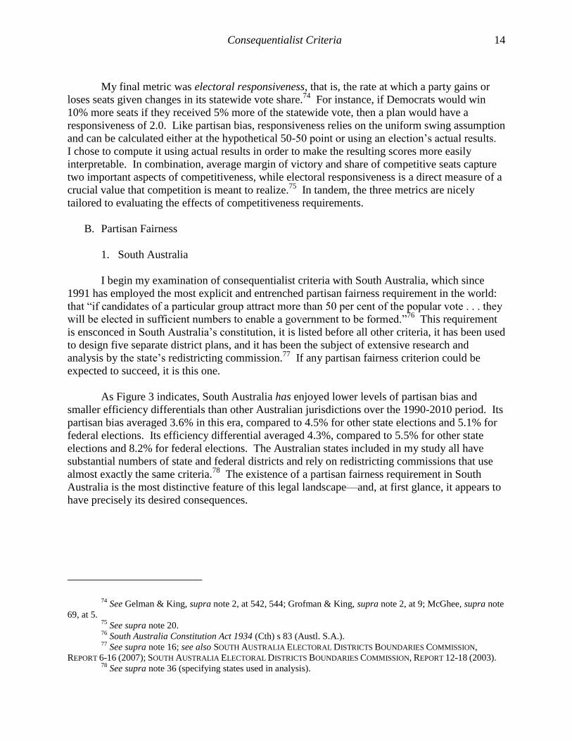
As Figure 3 indicates, South Australia has enjoyed lower levels of partisan bias and
smaller efficiency differentials than other Australian jurisdictions over the 1990-2010 period. Its
partisan bias averaged 3.6% in this era, compared to 4.5% for other state elections and 5.1% for
federal elections. Its efficiency differential averaged 4.3%, compared to 5.5% for other state
elections and 8.2% for federal elections. The Australian states included in my study all have
substantial numbers of state and federal districts and rely on redistricting commissions that use
almost exactly the same criteria.78
The existence of a partisan fairness requirement in South
Australia is the most distinctive feature of this legal landscape—and, at first glance, it appears to
have precisely its desired consequences.
74
See Gelman & King, supra note 2, at 542, 544; Grofman & King, supra note 2, at 9; McGhee, supra note
69, at 5. 75
See supra note 20. 76
South Australia Constitution Act 1934 (Cth) s 83 (Austl. S.A.). 77
See supra note 16; see also SOUTH AUSTRALIA ELECTORAL DISTRICTS BOUNDARIES COMMISSION,
REPORT 6-16 (2007); SOUTH AUSTRALIA ELECTORAL DISTRICTS BOUNDARIES COMMISSION, REPORT 12-18 (2003). 78
See supra note 36 (specifying states used in analysis).

15 Consequentialist Criteria
FIGURE 3: AUSTRALIAN PARTISAN BIAS SCORES AND EFFICIENCY DIFFERENTIALS, 1990-2010
However, the differences in partisan bias and the efficiency differential between South
Australia and other Australian jurisdictions do not rise to the level of statistical significance.79
Nor, when I carry out regressions with controls added for the year, the level of the election (state
or federal), the number of districts in a state, and the Australian Labor Party’s (ALP) share of the
statewide vote, does the presence of a partisan fairness requirement remain a significant predictor
of partisan bias or the efficiency differential.80
Interestingly, no variable seems to predict
partisan bias with any particular accuracy, perhaps because its levels are uniformly low thanks to
the use of independent redistricting commissions throughout Australia. However, the ALP’s
statewide vote share is linked negatively to the efficiency differential, perhaps because ALP
supporters are concentrated in urban areas, and so if the ALP’s vote share is low it is likely to
receive particularly few seats (and to waste particularly many votes).81
Also of note, the
presence of a partisan fairness requirement is statistically significant at the more generous 10%
level, indicating that it is likely having some downward influence on the efficiency differential.82
79
A two-sample t-test for partisan bias yields t = 0.76 and p = 0.23. A two-sample t-test for the efficiency
differential yields t = 1.12 and p = 0.13. 80
See infra app. tbl. 1. All of the regressions that I ran for this paper used ordinary least squares. All of the
regressions also used the election-year (i.e., an election by a given state in a given year) as the basic unit of analysis.
Since the presence of a partisan fairness requirement was not statistically significant even with these few controls
included, I did attempt to compile the full set of controls that I used for the U.S. models. In any case, redistricting
criteria and the institutions responsible for redistricting do not vary appreciably from state to state in Australia. 81
See supra note 14 (noting the tendency of single-member district plans to disadvantage leftist parties). 82
Its coefficient is substantial as well; the presence of a partisan fairness requirement reduces the efficiency
differential by 5.6%. However, this result ceases to hold when fixed effects for the state and year are included in the
model.
0%
1%
2%
3%
4%
5%
6%
7%
8%
9%
South Australia Other states Federal elections
Partisan bias Efficiency differential

Consequentialist Criteria 16
Longitudinal analysis further confirms that South Australia’s partisan fairness
requirement has not been very impactful. For much of the postwar era, malapportionment and
gerrymandering were rampant in the state; as Figure 4 displays, bias averaged 9.0% over the ten
elections between 1950 and 1975.83
In 1975, the state embraced the one-person, one-vote rule
and instituted an independent redistricting commission.84
Dramatic drops followed in both
partisan bias (9.0% to 3.6%) and the efficiency differential (5.7% to 2.7%) over the next five
elections. However, the 1991 adoption of the partisan fairness requirement did not produce any
further benefits. Partisan bias remained static over the next five elections (3.6% to 3.6%), while
the efficiency differential actually increased somewhat (2.7% to 4.3%). The upshot is that
equally sized districts and an independent commission improved partisan fairness in South
Australia, but an actual partisan fairness requirement did not. All of South Australia’s gains
came after its first round of redistricting reform—but before its second.
FIGURE 4: SOUTH AUSTRALIAN PARTISAN BIAS SCORES AND EFFICIENCY DIFFERENTIALS,
1950-2010
83
Because I wanted the bias scores to reflect the impact of South Australia’s pre-1975 malapportionment, I
calculated statewide vote shares here using aggregate vote tallies, not by averaging the parties’ district-specific vote
shares. For the same reason, I calculated the efficiency differentials using district-specific vote tallies, not vote
shares. See supra notes 68-69. 84
See SOUTH AUSTRALIA STATE ELECTORAL OFFICE, supra note 37, at 7. The first election conducted
under the new regime was in 1977.
0%
1%
2%
3%
4%
5%
6%
7%
8%
9%
10%
1950-1975 1977-1989 1993-2010
Partisan bias Efficiency differential

17 Consequentialist Criteria
2. U.S. House of Representatives
I turn next to the United States House of Representatives, where partisan fairness
requirements have been employed by eleven states in sixty elections since 1966. The decisions
to use these requirements typically have been made by courts that have found themselves
responsible for drawing district lines. Legislatures and commissions rarely have opted to take
partisan fairness into account.85
As Figure 5’s density curves indicate, both partisan bias and the efficiency differential are
lower in elections in which partisan fairness requirements are used. Partisan bias averages 6.2%
in elections with these criteria but 8.3% in elections without them. Similarly, the efficiency
differential averages 7.2% in elections with these criteria but 10.2% in elections without them.
Both of these differences are statistically significant.86
The density curves also illustrate why
partisan bias and the efficiency differential are lower in elections with partisan fairness
requirements. In both cases, the right tail of the no-requirement distribution, containing elections
with particularly high partisan bias and efficiency differential scores, is absent from the
distribution of elections with the criteria. In other words, the presence of a partisan fairness
requirement seems to prevent the adoption of district plans that are marked by extreme biases or
efficiency differentials.
FIGURE 5: DENSITY CURVES FOR U.S. HOUSE ELECTIONS, PARTISAN BIAS SCORES AND
EFFICIENCY DIFFERENTIALS, 1966-2012
As with the initial South Australian results, these findings appear positive at first glance.
Congressional elections with partisan fairness requirements indeed treat the major parties more
symmetrically than congressional elections without them. Unfortunately, as with South
Australia, the findings’ impressiveness decreases when the data is subjected to more rigorous
analysis. I regressed partisan bias and the efficiency differential against the presence of a
85
See supra fig. 1. 86
A two-sample t-test for partisan bias yields t = 2.83 and p = 0.004. A two-sample t-test for the efficiency
differential yields t = 3.55 and p = 0.0005. I omit states with fewer than five congressional districts from my
analysis because partisan fairness metrics are too unreliable when the number of districts is so small.
Consequentialist Criteria 18
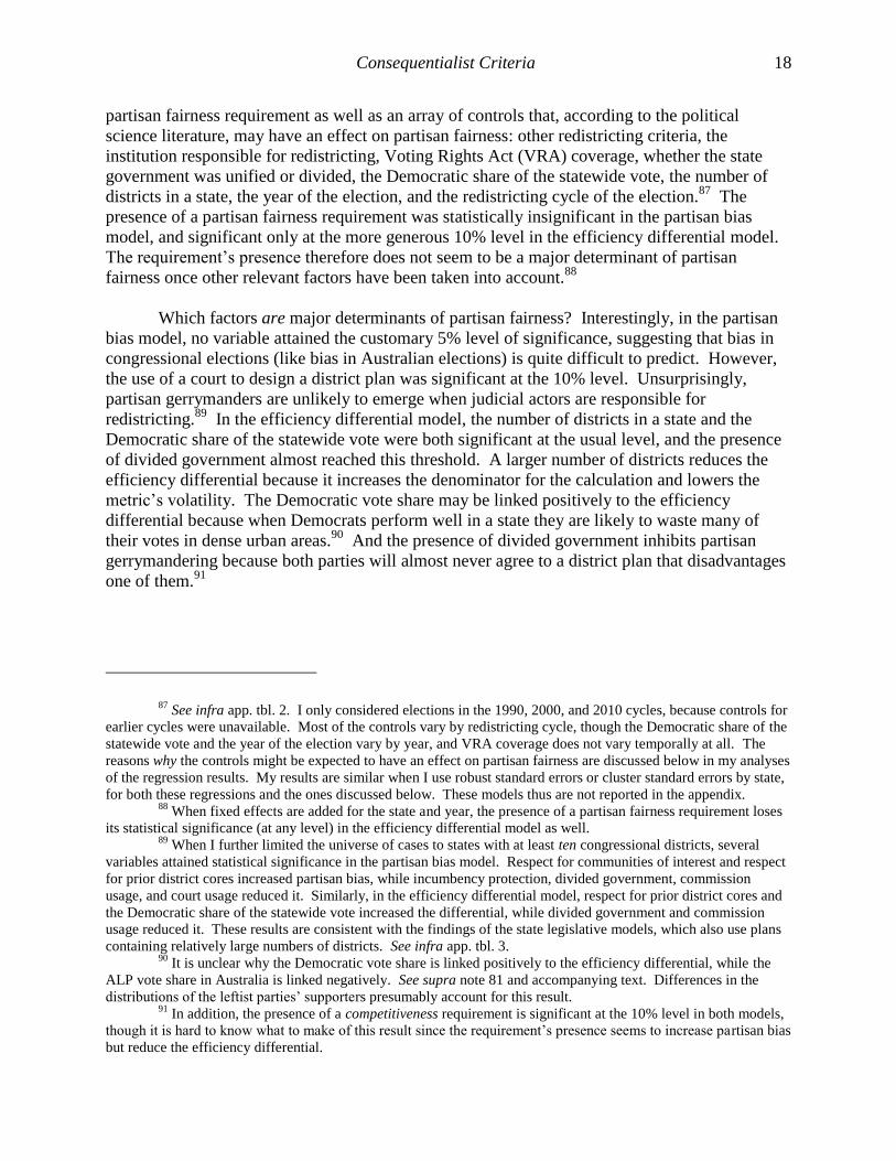
partisan fairness requirement as well as an array of controls that, according to the political
science literature, may have an effect on partisan fairness: other redistricting criteria, the
institution responsible for redistricting, Voting Rights Act (VRA) coverage, whether the state
government was unified or divided, the Democratic share of the statewide vote, the number of
districts in a state, the year of the election, and the redistricting cycle of the election.87
The
presence of a partisan fairness requirement was statistically insignificant in the partisan bias
model, and significant only at the more generous 10% level in the efficiency differential model.
The requirement’s presence therefore does not seem to be a major determinant of partisan
fairness once other relevant factors have been taken into account.88
Which factors are major determinants of partisan fairness? Interestingly, in the partisan
bias model, no variable attained the customary 5% level of significance, suggesting that bias in
congressional elections (like bias in Australian elections) is quite difficult to predict. However,
the use of a court to design a district plan was significant at the 10% level. Unsurprisingly,
partisan gerrymanders are unlikely to emerge when judicial actors are responsible for
redistricting.89
In the efficiency differential model, the number of districts in a state and the
Democratic share of the statewide vote were both significant at the usual level, and the presence
of divided government almost reached this threshold. A larger number of districts reduces the
efficiency differential because it increases the denominator for the calculation and lowers the
metric’s volatility. The Democratic vote share may be linked positively to the efficiency
differential because when Democrats perform well in a state they are likely to waste many of
their votes in dense urban areas.90
And the presence of divided government inhibits partisan
gerrymandering because both parties will almost never agree to a district plan that disadvantages
one of them.91
87
See infra app. tbl. 2. I only considered elections in the 1990, 2000, and 2010 cycles, because controls for
earlier cycles were unavailable. Most of the controls vary by redistricting cycle, though the Democratic share of the
statewide vote and the year of the election vary by year, and VRA coverage does not vary temporally at all. The
reasons why the controls might be expected to have an effect on partisan fairness are discussed below in my analyses
of the regression results. My results are similar when I use robust standard errors or cluster standard errors by state,
for both these regressions and the ones discussed below. These models thus are not reported in the appendix. 88
When fixed effects are added for the state and year, the presence of a partisan fairness requirement loses
its statistical significance (at any level) in the efficiency differential model as well. 89
When I further limited the universe of cases to states with at least ten congressional districts, several
variables attained statistical significance in the partisan bias model. Respect for communities of interest and respect
for prior district cores increased partisan bias, while incumbency protection, divided government, commission
usage, and court usage reduced it. Similarly, in the efficiency differential model, respect for prior district cores and
the Democratic share of the statewide vote increased the differential, while divided government and commission
usage reduced it. These results are consistent with the findings of the state legislative models, which also use plans
containing relatively large numbers of districts. See infra app. tbl. 3. 90
It is unclear why the Democratic vote share is linked positively to the efficiency differential, while the
ALP vote share in Australia is linked negatively. See supra note 81 and accompanying text. Differences in the
distributions of the leftist parties’ supporters presumably account for this result. 91
In addition, the presence of a competitiveness requirement is significant at the 10% level in both models,
though it is hard to know what to make of this result since the requirement’s presence seems to increase partisan bias
but reduce the efficiency differential.

19 Consequentialist Criteria
3. U.S. State Legislatures
American state legislative elections are the final set of races that I examine for evidence
of the effectiveness of partisan fairness requirements. Nine states have employed such
requirements in 128 state house and state senate elections over the 1967-2010 period.
Legislatures and courts each account for about half of these cases; the only state-level
commission to take partisan fairness into account is New Jersey’s.92
For present purposes, the
most notable difference between state legislative and congressional elections is the larger number
of districts in the former. The average state legislative plan has 66 districts, compared to 13 in
the congressional plans that I used in my analysis (and 9 in all congressional plans).93
The
greater volume of state legislative districts makes measures of both partisan fairness and
competitiveness substantially more trustworthy.
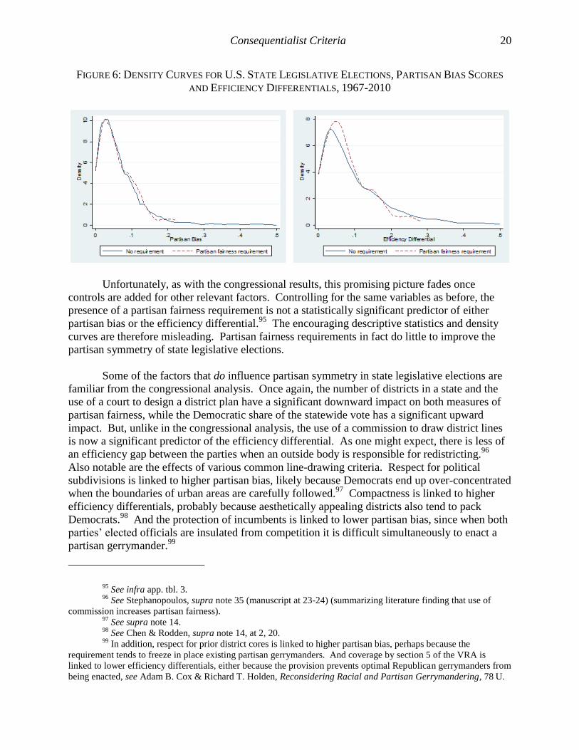
As Figure 6’s density curves display, both partisan bias and the efficiency differential are
lower in elections in which partisan fairness requirements are used. Partisan bias averages 5.9%
in elections with these criteria but 6.7% in elections without them. Similarly, the efficiency
differential averages 7.9% in elections with these criteria but 9.9% in elections without them.
Both of these differences are statistically significant.94
These state legislative findings are very
similar to the congressional results presented above, and so too are the shapes of the density
curves. Once again, the right tails of the no-requirement distributions, containing elections with
particularly high partisan bias and efficiency differential scores, are absent from the distributions
of elections with the criteria. The effect is even more pronounced here because the left sides of
the distributions are nearly identical. Partisan fairness requirements appear to alter the
distributions of state legislative plans only by slicing off their right tails.
92
See supra fig. 1. 93
See notes 86, 101 (noting that congressional regression analysis only considered plans with at least five
districts). 94
A two-sample t-test for partisan bias yields t = 1.88 and p = 0.031. A two-sample t-test for the efficiency
differential yields t = 3.35 and p = 0.0005. I omit states with multimember districts from my analysis because
partisan fairness metrics cannot easily be calculated for plans that use such districts.
Consequentialist Criteria 20
FIGURE 6: DENSITY CURVES FOR U.S. STATE LEGISLATIVE ELECTIONS, PARTISAN BIAS SCORES
AND EFFICIENCY DIFFERENTIALS, 1967-2010
Unfortunately, as with the congressional results, this promising picture fades once
controls are added for other relevant factors. Controlling for the same variables as before, the
presence of a partisan fairness requirement is not a statistically significant predictor of either
partisan bias or the efficiency differential.95
The encouraging descriptive statistics and density
curves are therefore misleading. Partisan fairness requirements in fact do little to improve the
partisan symmetry of state legislative elections.
Some of the factors that do influence partisan symmetry in state legislative elections are
familiar from the congressional analysis. Once again, the number of districts in a state and the
use of a court to design a district plan have a significant downward impact on both measures of
partisan fairness, while the Democratic share of the statewide vote has a significant upward
impact. But, unlike in the congressional analysis, the use of a commission to draw district lines
is now a significant predictor of the efficiency differential. As one might expect, there is less of
an efficiency gap between the parties when an outside body is responsible for redistricting.96
Also notable are the effects of various common line-drawing criteria. Respect for political
subdivisions is linked to higher partisan bias, likely because Democrats end up over-concentrated
when the boundaries of urban areas are carefully followed.97
Compactness is linked to higher
efficiency differentials, probably because aesthetically appealing districts also tend to pack
Democrats.98
And the protection of incumbents is linked to lower partisan bias, since when both
parties’ elected officials are insulated from competition it is difficult simultaneously to enact a
partisan gerrymander.99
95
See infra app. tbl. 3. 96
See Stephanopoulos, supra note 35 (manuscript at 23-24) (summarizing literature finding that use of
commission increases partisan fairness). 97
See supra note 14. 98
See Chen & Rodden, supra note 14, at 2, 20. 99
In addition, respect for prior district cores is linked to higher partisan bias, perhaps because the
requirement tends to freeze in place existing partisan gerrymanders. And coverage by section 5 of the VRA is
linked to lower efficiency differentials, either because the provision prevents optimal Republican gerrymanders from
being enacted, see Adam B. Cox & Richard T. Holden, Reconsidering Racial and Partisan Gerrymandering, 78 U.

21 Consequentialist Criteria
C. Competitiveness
1. U.S. House of Representatives
Competitiveness requirements are the other kind of consequentialist criteria, and they
have been employed at the congressional level by seven states in thirty-eight elections. Courts
are the institutions that most often have decided to impose these requirements, though they also
have been applied by commissions and, on one occasion, a legislature. Most of the states that
have used the requirements are located in the western part of the country.100
Like partisan fairness criteria, competitiveness requirements appear at first to have
produced their desired consequences. The average margin of victory is lower in elections with
them than in elections without them (32.0% versus 40.1%); the proportion of races decided by
less than twenty points is higher (37.6% versus 28.2%); and the level of electoral responsiveness
is higher as well (1.85 versus 1.44). All of these differences are statistically significant, though
only at the 10% level in the case of responsiveness.101
The density curves displayed in Figure 7
are less illuminating than the ones shown earlier, due to the relatively small number of
congressional elections with competitiveness requirements, but they also tend to confirm this
rosy picture. The average-margin-of-victory curve for elections with the criteria is clearly to the
left of the curve for elections without them, while the share-of-competitive-districts curve for
elections with the criteria is clearly to the right of the curve for elections without them.102
CHI. L. REV. 553, 573-74 (2011), or because Democrats are more efficiently distributed in the southern states
covered by section 5, see Chen & Rodden, supra note 14, at 30. 100
See supra fig. 1. 101
A two-sample t-test for average margin of victory yields t = 3.37 and p = 0.0009. A two-sample t-test
for the share of districts decided by less than twenty points yields t = -2.57 and p = 0.0074. And a two-sample t-test
for electoral responsiveness yields t = -1.50 and p = 0.071. As before, I omit states with fewer than five
congressional districts from my analysis because competitiveness metrics are too unreliable when the number of
districts is so small. See supra note 86. 102
On the other hand, the contrasts between the two electoral responsiveness distributions are not readily
apparent. This is unsurprising since the difference between the two distributions’ means is significant only at the
more generous 10% level. See supra note 101.

Consequentialist Criteria 22
FIGURE 7: DENSITY CURVES FOR U.S. HOUSE ELECTIONS, AVERAGE MARGIN OF VICTORY, SHARE
OF COMPETITIVE DISTRICTS, AND ELECTORAL RESPONSIVENESS, 1966-2012
Unfortunately, like the partisan fairness findings discussed above, these results evaporate
when controls are added for other factors that the political science literature suggests are
relevant. I regressed all three competitiveness metrics against the presence of a competitiveness
requirement as well as controls for other redistricting criteria, the institution responsible for
redistricting, VRA coverage, whether the state government was unified or divided, the
Democratic share of the statewide vote, the number of districts in a state, the year of the election,
and the redistricting cycle of the election.103
In none of these models does the presence of a
competitiveness requirement attain statistical significance at any level. In other words, efforts by
line-drawers to make congressional elections more competitive do not in fact result in
meaningful improvements in competition.
One factor that does have a meaningful impact on all three measures of competitiveness
is the use of a commission to draw district lines. Commission-drawn plans boast lower margins
103
See infra app. tbl. 4. As before, I only considered elections in the 1990, 2000, and 2010 cycles, because
controls for earlier cycles were unavailable. See supra note 87. Unsurprisingly, the presence of a competitiveness
requirement also fails to attain statistical significance when fixed effects are added for the state and year.
23 Consequentialist Criteria
of victory, higher shares of competitive districts, and higher levels of responsiveness,
presumably because their authors have no reason to prioritize the protection of incumbents.104
Respect for political subdivisions also has a pro-competitive effect in all three models, probably
because challengers are better able to convey their messages to voters in districts that are
congruent with towns or counties.105
On the other hand, VRA coverage increases the average
margin of victory and decreases both the share of competitive districts and responsiveness. Both
the majority-minority districts required by the VRA and the “bleached” districts adjacent to them
are particularly safe for incumbents. The presence of a compactness requirement also reduces
the share of competitive districts and responsiveness, perhaps because compact districts pack
Democrats without producing the countervailing benefits of district-subdivision congruence.106
2. U.S. State Legislatures
Finally, competitiveness requirements have been employed by seven states in sixty-five
state legislative elections. Commissions are the institutions that most often have decided to
impose these requirements, though they also have been applied by courts and, on one occasion, a
legislature. Most of the states that have used the requirements are again located in the West.107
As noted earlier, state legislative plans usually have many more districts than congressional
plans, a fact that makes calculations of both partisan fairness and competitiveness substantially
more reliable for the former.108
As with congressional elections, descriptive statistics tell quite a positive story about the
impact of competitiveness requirements at the state legislative level. The average margin of
victory is lower in elections with them than in elections without them (42.0% versus 50.7%); the
proportion of races decided by less than twenty points is higher (34.8% versus 29.8%); and the
level of electoral responsiveness is higher as well (1.93 versus 1.54). All of these differences are
statistically significant.109
The density curves displayed in Figure 8 also are more striking than
their congressional equivalents. It is now evident that the average-margin-of-victory curve for
elections with competitiveness criteria is to the left of the curve for elections without them; that
the share-of-competitive-districts curve for elections with the criteria is to the right of the curve
104
See Stephanopoulos, supra note 35 (manuscript at 24-25) (summarizing literature finding that
commission usage increases responsiveness and has indeterminate effects on competitiveness). 105
See id. (manuscript at 42, 46-47) (summarizing literature consistent with this result). 106
In addition, the Democratic share of the statewide vote is linked positively to the average margin of
victory, though only at the 10% level. This may be because when Democrats do particularly well in a state many of
their votes are cast in very safe urban districts. See supra note 14. The 2000 cycle also seems to have been
especially uncompetitive, as the dummy variable for this cycle was linked negatively to the share of competitive
districts. Lastly, unlike with the partisan fairness models, the regression results lose their intelligibility when the
universe of cases is further limited to states with at least ten congressional districts. See supra note 89. This is
because most states that have used competitiveness requirements have had fewer than ten districts. 107
See supra fig. 1. 108
See supra text accompanying note 93. 109
A two-sample t-test for average margin of victory yields t = 5.86 and p = 0.0000. A two-sample t-test
for the share of districts decided by less than twenty points yields t = -3.49 and p = 0.0004. And a two-sample t-test
for electoral responsiveness yields t = -3.67 and p = 0.0002. As before, I omit states with multimember districts
from my analysis because competitiveness metrics cannot easily be calculated for plans that use such districts. See
supra note 94.

Consequentialist Criteria 24
for elections without them; and that the responsiveness curve for elections with the criteria is
also to the right of the curve for elections without them. In the last two plots, the use of
competitiveness criteria seems cleanly to shift the entire distribution to the right, in the direction
of greater competition.
FIGURE 8: DENSITY CURVES FOR U.S. STATE LEGISLATIVE ELECTIONS, AVERAGE MARGIN OF
VICTORY, SHARE OF COMPETITIVE DISTRICTS, AND ELECTORAL RESPONSIVENESS, 1967-2010
In all of the analysis to this point, the presence of a consequentialist criterion was
statistically insignificant, or significant only at the 10% level, when controls were added for
other relevant factors. Here, however, the presence of a competitiveness requirement remains a
significant predictor of the average margin of victory (at the 10% level), the share of competitive
districts, and the level of electoral responsiveness after I control for the usual array of variables.
This is the only potential success for consequentialist criteria identified by this paper. In state
legislative elections (but not in congressional elections), competitiveness criteria (but not
partisan fairness criteria) may indeed result in their desired consequences. Controlling for other

25 Consequentialist Criteria
pertinent factors, they decrease the average margin of victory (by 4.0%) and increase the
proportion of competitive districts (by 5.1%) as well as the level of responsiveness (by 0.40).110
Several other factors also have significant effects on competitiveness. As in the
congressional analysis, respect for political subdivisions has a pro-competitive impact in all three
models, while VRA coverage has an anti-competitive influence in each case. The use of a court
to draw district lines also increases competitiveness in every model. Like commissions, courts
have no particular incentive to shield incumbents from electoral challenges. On the other hand,
respect for prior district cores, incumbent protection requirements, and the presence of divided
government all are linked to reduced competition. Incumbents tend to benefit when their
districts are kept largely intact after a round of redistricting. They are even more heavily
advantaged when their protection is made an explicit line-drawing criterion. And when
government is divided, both parties are motivated to shelter their elected officials, thus
suppressing competition, since they lack the ability to enact a partisan gerrymander.111
III. IMPLICATIONS
The empirical results reported above have important implications both for the partisan
fairness and competitiveness approaches and for redistricting reform in general. It is to these
implications that I turn in this Part. With respect to the two consequentialist approaches, the
dominant theme of the analysis is their inability to produce their desired consequences.
However, there are some grounds for optimism in the efficiency differential models and in the
competitiveness models for state legislative elections. Consequentialist criteria may usually be
ineffective because of their poor drafting, low prioritization, and need for unrealistically accurate
electoral forecasting. But they do enjoy some success in reducing the efficiency differential
(probably a better metric than partisan bias), and in increasing the competitiveness of state
legislative elections (probably the domain best suited to consequentialist line-drawing).
With respect to redistricting reform generally, the clearest point to emerge is the strong
performance of neutral institutions. In both South Australia and the United States, the use of
independent commissions is linked to greater partisan fairness and greater competitiveness. The
use of courts to draw district lines in the United States has similarly positive consequences.
Accordingly, institutional change should be a higher-priority goal for reformers than the
adoption of consequentialist approaches. The second point conveyed by the data is the unclear
efficacy (or worse) of many redistricting criteria. For example, compactness requirements
110
See infra tbl. 5. These results persist when fixed effects are added for the year of the election, but they
cease to hold when fixed effects are added for both the state and year. The results also hold when I use robust
standard errors (at the 5% level for each metric), but they hold only for responsiveness when I cluster standard errors
by state. See supra note 87 (discussing use of robust and clustered standard errors). 111
In addition, as in the congressional analysis, the Democratic share of the statewide vote is linked to
lower competitiveness. See supra note 106. The number of districts in a state is also linked to lower
competitiveness, perhaps because when districts are especially small in population it is difficult for them to be
competitive. Consistent with findings that competition is decreasing in state legislative elections, the election year
has an anti-competitive effect as well. See Niemi et al., supra note 72, at 64-67. Lastly, respect for communities of
interest is linked to higher electoral responsiveness, while compactness and partisan fairness requirements are linked
to lower responsiveness.

Consequentialist Criteria 26
reduce both partisan fairness and competitiveness; respect for communities of interest has almost
no effect on any of the relevant metrics; and the pro-competitive impact of respect for political
subdivisions must be balanced against the criterion’s link to lower partisan fairness. Institutional
change thus should also be a higher-priority goal than the enactment of conventional line-
drawing requirements.
A. Consequentialist Approaches
The overarching conclusion of the above empirical analysis was that, once other relevant
factors have been taken into account, consequentialist criteria have not achieved their desired
results. The differences in partisan bias and the efficiency differential between South Australia
and other Australian jurisdictions were not statistically significant. Nor did South Australia
experience any increases in partisan symmetry after adopting its partisan fairness requirement in
1991. In the United States, the presence of a partisan fairness criterion also did not have a
significant impact on partisan bias or the efficiency differential after controls for pertinent
variables were added. In the regression models for congressional elections, competitiveness was
unaffected as well by the presence of a competitiveness requirement.112
What accounts for this unimpressive record? Why don’t consequentialist criteria seem to
work? One answer is that they are often drafted so poorly that it is difficult to discern what their
authors sought to accomplish or how they are meant to be enforced. For example, statutes in
Delaware and Hawaii forbid district plans that “unduly favor” a political party.113
It is entirely
unclear how partisan favoritism is supposed to be determined, let alone what level of favoritism
is undue. Similarly, authorities in California, New York, and Virginia have taken “political
fairness” into account in designing district plans, but without providing any definition of this
exceedingly vague term.114
And statements that competitiveness was “considered,” as in
Colorado, Florida, and Wisconsin, neither explain what kind of competition was examined, nor
specify how serious the consideration was.115
It is not too surprising that consequentialist criteria
of such imprecision have been relatively ineffective.
Another explanation for the weak record of consequentialist criteria is the low priority
they often have been accorded relative to other requirements. For instance, courts in California,
Colorado, Michigan, Texas, and Wisconsin designed district plans largely on the basis of non-
consequentialist criteria, and then took partisan fairness into account only after provisional
districts already had been drawn.116
As the Texas court commented in its discussion of its line-
drawing methodology, “Finally, we checked our plan against the test of general partisan
112
And even the limited successes of the efficiency differential models and the competitiveness models in
state legislative elections disappeared after fixed effects were added for the state and year. See supra notes 82, 88,
95, 110. 113
See supra fig. 1. 114
See id. 115
See supra fig. 2. 116
See Balderas v. Texas, 2001 WL 36403750, at *3 (E.D. Tex. Nov. 14, 2001); Good v. Austin, 800 F.
Supp. 557, 566-67 (E.D. Mich. 1992); Prosser v. Elections Bd., 793 F. Supp. 859, 871 (W.D. Wis. 1992);
Legislature v. Reinecke, 516 P.2d 6, 38 (Cal. 1973); Avalos v. Davidson, 2002 WL 1895406, at *8 (Colo. Dist. Ct.
Jan. 25, 2002).

27 Consequentialist Criteria
outcome.”117
Analogously, the relevant Arizona and Wisconsin laws both make clear that
competitiveness is subordinate to other redistricting criteria. The Arizona constitution declares
that “[t]o the extent practicable, competitive districts should be favored where to do so would
create no significant detriment to the other goals,”118
while the Wisconsin statute states that
“[t]o the very limited extent that precise population equality is unattainable, [the district plans] .
. . giv[e] due consideration to . . . competitive legislative districts.”119
Again, it is unsurprising
that consequentialist criteria that have been granted such low priority have had such limited
effects.
A further reason why consequentialist criteria have not been very effective is that election
results—and in particular how they translate into measures of partisan fairness and
competitiveness—are quite difficult to forecast. In U.S. congressional elections, for example,
the correlation between the Democratic share of the statewide vote in one election and the
Democratic share in the previous election averaged 0.80 between 1968 and 2010. But the
correlations for average margin of victory, share of competitive districts, responsiveness, and the
efficiency differential averaged only 0.63, 0.42, 0.24, and 0.45, respectively, over the same
period. These figures reveal a sufficiently high level of volatility that it is hard to see how even
the best-written and most highly-prioritized consequentialist criteria could consistently achieve
their desired results. Over the decade-long lifespan of a district plan, competitiveness and
partisan fairness tend to vary widely and unpredictably, thus undoing even quite meticulous
districting arrangements.120
The difficulty of predicting election results is also why South Australia’s partisan fairness
requirement has not functioned as well as might have been expected. As Jenni Newton-Farrelly
has explained, the South Australian commission relies on past election results as well as the
uniform swing assumption to design its district plans.121
This approach worked well for the four
elections between 1993 and 2006, in which candidates associated with the party that won a
majority of the statewide vote always won a majority of the statewide seats.122
However, the
commission’s efforts misfired dramatically in 2010, when the ALP received 48.4% of the
117
Balderas, 2001 WL 36403750, at *3 (emphasis added). 118
ARIZ. CONST. art. IV, pt. 2, § 1(14)(F) (emphasis added). 119
WIS. STAT. § 4.001(3) (repealed 2011) (emphasis added). 120
I did not include elections held under different district plans than the previous elections (i.e., 1972, 1982,
1992, 2002, and 2012). I also did not include district plans with fewer than five districts. Partisan bias is the one
metric that does seem to be quite predictable, with an average correlation of 0.86 from election to election. The
equivalent correlations for state legislative elections are 0.81 for average margin of victory, 0.64 for share of
competitive districts, 0.54 for responsiveness, 0.48 for partisan bias, and 0.51 for the efficiency differential. When I
ran the various regression models using only elections held immediately after a round of redistricting, more of the
variance was explained in each case, but the presence of consequentialist criteria was no more significant. Line-
drawers thus seem unable to increase partisan fairness or competitiveness even in elections that are held just months
after their district plans have been completed. Cf. Gelman & King, supra note 2, at 548, 550 (finding that bias tends
to be stickier over time than responsiveness in state legislative elections). 121
See Newton-Farrelly, Gerry-Built, supra note 16, at 475-80 (discussing South Australian commission’s
methodology). 122
Though in 2002 a third-party member who was expected to support the Liberals actually voted for a
Labor government, thus giving Labor control of the state parliament even though the party had received a minority
of the statewide vote. See Newton-Farrelly, Wrong Winner, supra note 16, at 3-4.

Consequentialist Criteria 28
statewide vote but 57.4% of the statewide seats, resulting in a partisan bias of 7.4% and an
efficiency differential of 10.6%. What went wrong was that the ALP’s vote share did not swing
uniformly across all districts. Instead, “[t]he ALP ran the most successful defensive marginal
seats campaign seen in South Australia,” so that “the biggest swings occurred in safe Labor seats
and in fairly safe Liberal seats,” while marginal Labor seats barely swung at all.123
Not even the
world’s best partisan fairness requirement could succeed in the face of such clever campaign
tactics and unequal resulting swings.
A final possibility is that consequentialist criteria do work but the metrics I calculated
were too unreliable or the analytical techniques I used were too crude to pick up their effects. I
estimated partisan fairness and competitiveness using standard measures of the two concepts as
well as data from actual legislative elections. It is plausible that more advanced metrics (e.g.,
partisan bias computed without reliance on the uniform swing assumption124
) or other data (e.g.,
presidential election results aggregated by district125
) would have led to different conclusions.
Similarly, I sought to determine the effects of consequentialist criteria using conventional OLS
regressions that included controls for relevant variables. It is again plausible that the results
would have been different had I used other analytical techniques (e.g., difference-in-differences
analysis126
) or additional controls (e.g., the geographic distribution of partisan support across a
state127
). However, my sense from experimenting with these and other approaches is that this
paper’s null findings are quite robust. Though I cannot be sure, I would be surprised if better
data or more sophisticated techniques would determine that consequential criteria actually are
successful.
A relative bright spot in this gloomy picture is the performance of partisan fairness
requirements in the efficiency differential models. In two of the three sets of elections that I
examined—Australian and U.S. congressional—the presence of a partisan fairness criterion was
statistically significant at the 10% level, even after controlling for other relevant factors.128
The
requirement’s presence reduced the efficiency differential by 5.6% in Australian elections and by
2.6% in U.S. congressional elections.129
Too much should not be made of these results, since the
requirement’s presence did not attain the standard 5% significance level. But it does seem that
partisan fairness criteria are not entirely useless, and it is also unsurprising that these criteria
would have a greater impact on the efficiency differential than on partisan bias. As discussed
above, the efficiency differential is calculated using actual election results rather than the
outcome of a hypothetical 50-50 election, and it takes into account wasted votes rather than gaps
123
Id. at 5; see also Newton-Farrelly, Blindfolds, supra note 16, at 3. 124
See Gelman & King, supra note 66, at 521-23. However, “the uniform partisan swing assumption does
hold approximately in a vast array of democratic elections in the U.S.” Grofman & King, supra note 2, at 11
(emphasis added). 125
See supra note 38. However, the regressions I ran using this data at the congressional level were less
illuminating, and presidential election results aggregated by district are unavailable at the state legislative level. 126
However, it is difficult to select appropriate jurisdictions and time periods for difference-in-differences
analysis, and my experiments with the technique did not yield any especially interesting results. 127
However, there is no well-accepted method for measuring this distribution. Cf. Stephanopoulos, supra
note 15, at 1936-41 (introducing technique for measuring spatial diversity of individual districts). 128
See infra tbls. 1-2. However, the requirement’s presence lost its statistical significance in both cases
once fixed effects were added for the state and year. See supra notes 82, 88. 129
See id.

29 Consequentialist Criteria
between the parties’ seats.130
According to its creator, Eric McGhee, these attributes make it a
more sensitive measure of partisan fairness than bias131
—and may explain why it responds to the
presence of a partisan fairness requirement while bias does not.
The more important exception to the poor record of consequentialist criteria is the
performance of competitiveness requirements in state legislative elections. Controlling for other
pertinent variables, the presence of a competitiveness requirement was linked to a statistically
significant decrease in the average margin of victory (by 4.0%) as well as statistically significant
increases in the share of competitive districts (by 5.1%) and the level of electoral responsiveness
(by 0.40).132
One explanation for this finding is that competitiveness may be easier to forecast
than partisan fairness. Measures of competitiveness are derived more directly from election
results than are measures of partisan fairness, which require the consideration of vote-seat
conversion as well.133
Predictable factors like incumbency also have a large influence on the
competitiveness of individual districts. Perhaps for these reasons, the correlations from election
to election in state legislative races were higher for all three competitiveness metrics I used than
for either metric of partisan fairness.134
The election level is the second potential explanation for the effectiveness of
competitiveness requirements in state legislative races. As noted earlier, state legislative plans
have many more districts than congressional plans, a fact that improves the reliability of electoral
metrics that are calculated for the former.135
This improved reliability explains why the state
legislative models all were able to explain more of the variance in the dependent variables than
the congressional models.136
It also explains why the metrics’ correlations from election to
election were generally higher in state legislative races than in congressional races.137
Beyond
their larger numbers of districts, the stakes are lower in state legislative elections as well. Most
state chambers are not closely divided between the parties, meaning that control of a chamber
rarely hinges on the effectiveness of a partisan gerrymander.138
Even where control of a chamber
does so hinge, it is only a single state house or state senate that is at stake—not the United States
House of Representatives. It may therefore be easier for state legislative line-drawers to
130
See supra notes 69-70 and accompanying text. 131
See McGhee, supra note 69, at 23-25. 132
See infra tbl. 5. However, the requirement’s presence also lost its statistical significance once fixed
effects were added for the state and year. See supra note 110. 133
This is particularly the case for average margin of victory and the share of competitive districts. Like
the partisan fairness metrics, responsiveness does require the consideration of vote-seat conversion, though using
actual election results rather than the outcome of a hypothetical 50-50 election. See supra note 74 and
accompanying text. 134
See supra note 120; see also Michael P. McDonald, Redistricting and Competitive Districts, in THE
MARKETPLACE OF DEMOCRACY, supra note 19, at 222, 238 (arguing, based on author’s own redistricting experience,
that “it is possible to devise a working definition of a competitive district that will foster competitive elections”). 135
See supra note 93 and accompanying text. 136
See infra tbls. 2-5. 137
See supra note 120. 138
Over the 1968-2010 period, the parties’ respective seat shares came within twenty points of each other
in state legislative chambers only about 40% of the time. In contrast, the parties’ respective seat shares in Congress
were this close about 80% of the time over the same period.
Consequentialist Criteria 30
prioritize consequentialist criteria than for their congressional counterparts. Lower stakes may
be conducive to the achievement of goals other than partisan or bipartisan advantage.139
In sum, the overall record of consequentialist criteria is poor, likely because of their
shoddy drafting, low prioritization, and need for unrealistically accurate electoral forecasts. But
there is a glimmer of hope in the ability of partisan fairness requirements to reduce the efficiency
differential in two of the three sets of elections that I studied. This ability likely stems from the
measure’s greater sensitivity relative to the more common partisan bias metric. And there is
even more reason for optimism in the performance of competitiveness requirements in state
legislative elections. Whether because competitiveness is easier to forecast than partisan
fairness, or because state legislative elections are a more favorable setting than congressional
elections, competition indeed is meaningfully more vigorous when district plans are designed
using competitiveness criteria.
B. Other Approaches
The analysis presented in Part II sheds light on not only the performance of
consequentialist approaches, but also the records of other popular proposals for redistricting
reform. The most common such proposal (and one that I have defended in earlier work140
) is the
use of independent institutions, such as commissions, to enact district plans. The reasoning is
that actors who are personally unaffected by redistricting should be able to draw better districts
than self-interested politicians. Neutral plans should command greater popular legitimacy, they
should better comply with whatever criteria apply to the line-drawing process—and they should
be fairer to the major parties and more competitive as well.141
Consistent with these expectations, South Australia experienced dramatic improvements
in both partisan fairness and competitiveness after adopting its independent commission in 1975.
As noted earlier, partisan bias fell from 9.0% in 1950-1975 to 3.6% in 1977-2010, while the
efficiency differential fell from 5.7% to 3.5%.142
Similarly, the average margin of victory fell
from 29.3% to 24.6%, the share of competitive districts rose from 33.1% to 42.7%, and the level
of electoral responsiveness rose from 1.4 to 2.2. Some of this progress is likely due to South
Australia’s simultaneous embrace of the one-person, one-vote rule, but some of it also must be
attributed to the state’s institutional reforms.
Another illuminating comparison is between all elections in Australia (where all states
use commissions) and elections in the United States. With respect to partisan fairness, as Figure
9 indicates, partisan bias has averaged 4.6% in Australia and the efficiency differential has
averaged 7.0%. The equivalent figures are 6.6% and 9.8% in U.S. state legislative elections, and
8.2% and 10.1% in U.S. congressional elections. With respect to competitiveness, as Figure 9
also displays, the average margin of victory has averaged 20.0% in Australia, the share of
139
See Cain et al., supra note 67, at 1 (noting that “redistricting [criteria] can be much more potent in the
larger number of state legislative districts”). 140
See Stephanopoulos, supra note 35 (manuscript at 20-28). 141
See id. (making these arguments). 142
See supra section II.B.1.

31 Consequentialist Criteria
competitive districts has averaged 55.3%, and the level of electoral responsiveness has averaged
2.84. The equivalent figures are 50.4%, 30.0%, and 1.55 in U.S. state legislative elections, and
39.7%, 28.7%, and 1.46 in U.S. congressional elections. These are stark differences, especially
for competitiveness, with Australia holding the advantage in every case. Australian and
American elections both use single-member districts, first-past-the-post voting, and the one-
person, one-vote rule, and they both are dominated by two parties. The most glaring difference
between the systems—the Australian embrace of redistricting commissions—thus likely
accounts for a good deal of the Australian edge in partisan fairness and competitiveness.
FIGURE 9: PARTISAN FAIRNESS AND COMPETITIVENESS METRICS FOR AUSTRALIAN AND
AMERICAN ELECTIONS
Further support for the efficacy of independent institutions comes from the various U.S.-
specific regression models. With respect to partisan fairness, commission usage had a
statistically significant downward impact on the efficiency differential in state legislative
elections (by 2.1%). Similarly, reliance on a court to draw district lines lowered partisan bias (by
1.3%) and the efficiency differential (by 2.7%) in state legislative elections, and partisan bias in
congressional elections too (by 2.0%).143
With respect to competitiveness, commission usage
reduced the average margin of victory (by 8.9%) and increased the share of competitive districts
(by 9.9%) and the level of electoral responsiveness (by 0.99) in congressional elections.
143
See infra tbls. 2-3.

Consequentialist Criteria 32
Analogously, reliance on a court reduced the average margin of victory (by 9.1%) and increased
the share of competitive districts (by 6.7%) and the level of electoral responsiveness (by 0.45) in
state legislative elections.144
The upshot is that in just about every model I considered, one of the
key causes of appealing electoral outcomes was the use of a commission or court to draw district
lines.
To be sure, this paper’s results do not present an airtight case for independent institutions.
It is unclear whether South Australia’s post-1975 gains should be attributed to its adoption of a
commission or its espousal of the one-person, one-vote rule. The Australian and American
electoral systems differ not only in their reliance on commissions, but also in their use of
mandatory voting (yes in Australia, no in America), their use of preferential voting (same), and
their basic structure (parliamentary versus presidential). And the coefficients for commission
and court usage in the U.S. regression models were often small, and there is no good explanation
why these factors varied in their significance from model to model. But despite these caveats,
the record of independent institutions is undeniably positive. To a much greater extent than
consequentialist criteria, they actually produce improvements in both partisan fairness and
competitiveness.145
Reformers concerned about electoral outcomes, both in America and abroad,
thus would be well-advised to focus their energies on institutional change, not the adoption of
outcome-oriented line-drawing requirements.
The other common proposal for redistricting reform is the enactment of conventional
criteria such as compactness, respect for political subdivisions, respect for communities of
interest, and respect for prior district cores.146
The logic is that if redistricting authorities must
abide by such requirements, they will be unable simultaneously to pursue partisan advantage or
suppress competition. Reduced discretion will produce better election results. In addition,
compliance with some of these criteria often is thought to have independent normative value.
For instance, several scholars (myself included147
) have argued that when districts are congruent
with communities of interest, voters are more motivated to participate in politics, and elected
officials are better able to represent their constituents.
This paper does not contribute to the debate about the participatory or representational
implications of conventional redistricting criteria. It does, however, offer several grounds for
skepticism as to the ability of these criteria to improve partisan fairness and competitiveness by
limiting line-drawers’ discretion. In the various U.S.-specific regression models, the record of
the criteria was mixed at best, and sometimes even counterproductive. Beginning with
compactness, all of its statistically significant effects were in an undesirable direction. The
presence of a compactness requirement increased the efficiency differential in state legislative
elections, reduced the share of competitive districts and the level of electoral responsiveness in
144
See infra tbls. 4-5. 145
This paper’s findings are confirmed by the existing political science literature. See Stephanopoulos,
supra note 35 (manuscript at 23-25) (summarizing work on implications of commission usage for partisan bias,
responsiveness, and competitiveness). 146
I also include data on incumbency protection in my regression models, but it is a less common criterion
and also one that clearly is not rooted in a desire to promote partisan fairness or competitiveness. 147
See Nicholas O. Stephanopoulos, Redistricting and the Territorial Community, 160 U. PA. L. REV. 1379,
1390-97 (2012); Stephanopoulos, supra note 15, at 1941-48.

33 Consequentialist Criteria
congressional elections, and reduced responsiveness in state legislative elections as well.148
Whatever the aesthetic benefits may be of compact districts, they apparently do not translate into
electoral improvements. To the contrary, compact districts tend to pack Democrats and to result
in unfair and uncompetitive district plans.
The situation is more ambiguous with respect for political subdivisions. The requirement
had a clear pro-competitive effect, reducing the average margin of victory and increasing the
share of competitive districts and the level of electoral responsiveness in both congressional and
state legislative elections.149
But the requirement also increased partisan bias in state legislative
elections.150
These results arguably are reconcilable because adherence to subdivision
boundaries may pack Democrats in certain districts (thus increasing partisan bias) while
generally making it easier for challengers to convey their messages to voters (thus increasing
competitiveness). But even if the results can be squared, they still present reformers with an
unwelcome choice between partisan fairness and competitiveness. Gains cannot be made along
both dimensions by mandating that districts coincide with political subdivisions.
Next, respect for communities of interest seems to be a largely toothless requirement, at
least in terms of its electoral consequences. The requirement had no meaningful impact on
partisan fairness, and its only statistically significant effect in the competitiveness models was to
increase responsiveness in state legislative elections.151
Earlier work of mine, using more
sophisticated conceptions of district-community congruence, has produced more favorable
results,152
but it does appear that the mere presence of a community-of-interest criterion is mostly
ineffectual. Finally, respect for prior district cores, like compactness, has only adverse effects.
The requirement increased partisan bias and the average margin of victory and decreased the
share of competitive districts and the level of electoral responsiveness in state legislative
elections.153
By freezing in place existing district plans, the requirement evidently advantages
incumbents who have thrived under the status quo and prevents partisan imbalances from being
corrected.
Once again, these findings should be taken with a grain of salt. Like consequentialist
criteria, conventional requirements are often poorly drafted and subordinate to other redistricting
considerations. It is quite possible that they would perform better if they were written more
clearly or prioritized more highly. Similarly, the presence of a requirement that districts be
designed in a certain manner does not guarantee that they actually will be drawn in this way.154
148
See infra tbls. 2-5. 149
See infra tbls. 4-5. 150
See infra tbl. 3. 151
See infra tbls. 2-5. 152
See Stephanopoulos, supra note 147, at 1459-62 (finding that community-of-interest requirement with
three gradations had positive implications for partisan bias and electoral responsiveness in 2002 state legislative
elections); Stephanopoulos, supra note 15, at 1963-66 (finding that spatial diversity, a proxy for district-community
congruence, is linked in expected directions to bias and responsiveness). 153
See infra tbls. 2-5. 154
See Jason Barabas & Jennifer Jerit, Redistricting Principles and Racial Representation, 4 STATE POL. &
POL’Y Q. 415, 428 (2004) (noting difficulty of assessing “the manner in which or even whether [redistricting criteria]
were implemented”); Forgette et al., Un-Principled Politics, supra note 35, at 13.

Consequentialist Criteria 34
District-community congruence itself, for example, may have very different consequences than
an ostensible rule that districts must respect communities of interest.155
Still, it is indisputable
that the record of conventional redistricting criteria is mediocre at best. Reformers who hope to
increase the partisan fairness and competitiveness of elections clearly should turn their attention
elsewhere—above all to improving the institutions responsible for redistricting.
CONCLUSION
The emergence of the partisan fairness and competitiveness approaches is arguably the
most important development of the last generation in the redistricting domain. But while much
scholarly attention has been devoted to the approaches’ theoretical merits, almost none has yet
been paid to a simpler (but perhaps more vital) question: How well do consequentialist criteria
actually work? This paper has sought to answer this query by compiling a comprehensive list of
jurisdictions that have used the criteria and then calculating measures of partisan fairness and
competitiveness for a large set of Australian and American elections. Unfortunately for their
proponents, the main finding of this analysis is that consequentialist criteria do not work very
well. Controlling for other relevant variables, they typically do not make elections meaningfully
fairer or more competitive.
Two bright spots in this picture are that consequentialist criteria do increase fairness
along one of the two metrics I used, and that they do increase competitiveness in U.S. state
legislative elections. An optimist may therefore be forgiven for speculation that the criteria
would perform even better if only they were drafted more precisely, prioritized more highly, or
based on better election forecasts. A more robust finding, however, is that electoral outcomes
actually can be improved by not taking electoral predictions directly into account.
Consequentialist criteria themselves are largely ineffective, but the use of independent
redistricting institutions, such as commissions and courts, is quite effective indeed. According to
data from both Australia and America, commission- and court-drawn plans are substantially
fairer and more competitive than plans devised by self-interested politicians. Ironically, it seems
that consequentialist criteria cannot achieve their own desired consequences—but that non-
consequentialist approaches can.
155
See supra note 152.

35 Consequentialist Criteria
APPENDIX
Table 1: Australia Partisan Fairness Models
Variables Model 1: Partisan Bias (Absolute
Value)
Model 2: Efficiency Differential
(Absolute Value)
Partisan fairness requirement -0.016 (0.021) -0.056 (0.033)*
Year -0.00056 (0.00062) -0.00035 (0.00096)
Level of election 0.0079 (0.022) 0.034 (0.034)
Number of districts -0.00021 (0.00035) -0.00089 (0.00054)
ALP share of two-party vote -0.036 (0.091) -0.47 (0.14)***
Constant 1.19 (1.24) 1.03 (1.93)
Observations 66 66
Adjusted R-Squared -0.039 0.23
Entries for variables take form: coefficient (standard error).
*** p < 0.01, ** p < 0.05, * p < 0.1

Consequentialist Criteria 36
Table 2: U.S. House of Representatives Partisan Fairness Models
Variables Model 1: Partisan Bias (Absolute
Value)
Model 2: Efficiency Differential
(Absolute Value)
Partisan fairness requirement -0.014 (0.015) -0.026 (0.015)*
Compactness requirement 0.0028 (0.012) -0.0023 (0.011)
Political subdivision preservation
requirement
0.0048 (0.014) 0.0034 (0.014)
Community of interest preservation
requirement
-0.0041 (0.016) -0.0045 (0.016)
Respect for prior district core
requirement
-0.0089 (0.015) -0.020 (0.015)
Incumbent protection requirement -0.0070 (0.018) -0.00089 (0.018)
Competitiveness requirement 0.029 (0.016)* -0.030 (0.016)*
Voting Rights Act coverage 0.011 (0.011) 0.0053 (0.011)
Legislature responsible – divided
government
-0.014 (0.011) -0.021 (0.011)*
Commission responsible -0.014 (0.014) 0.0057 (0.014)
Court responsible -0.020 (0.011)* 0.0082 (0.011)
Democratic share of two-party vote 0.0087 (0.040) 0.11 (0.040)***
Number of districts -0.00048 (0.00041) -0.0018 (0.00041)***
Year -0.00075 (0.0014) -0.00028 (0.0014)
2000 cycle 0.017 (0.016) 0.012 (0.016)
2010 cycle 0.040 (0.026) 0.024 (0.026)
Constant 1.59 (2.75) 0.64 (2.73)
Observations 334 334
Adjusted R-Squared 0.022 0.063
Entries for variables take form: coefficient (standard error).
*** p < 0.01, ** p < 0.05, * p < 0.1
Legislature responsible – unified government is the omitted institutional variable. 1990 cycle is
the omitted date variable.
Only states with at least five congressional districts included.
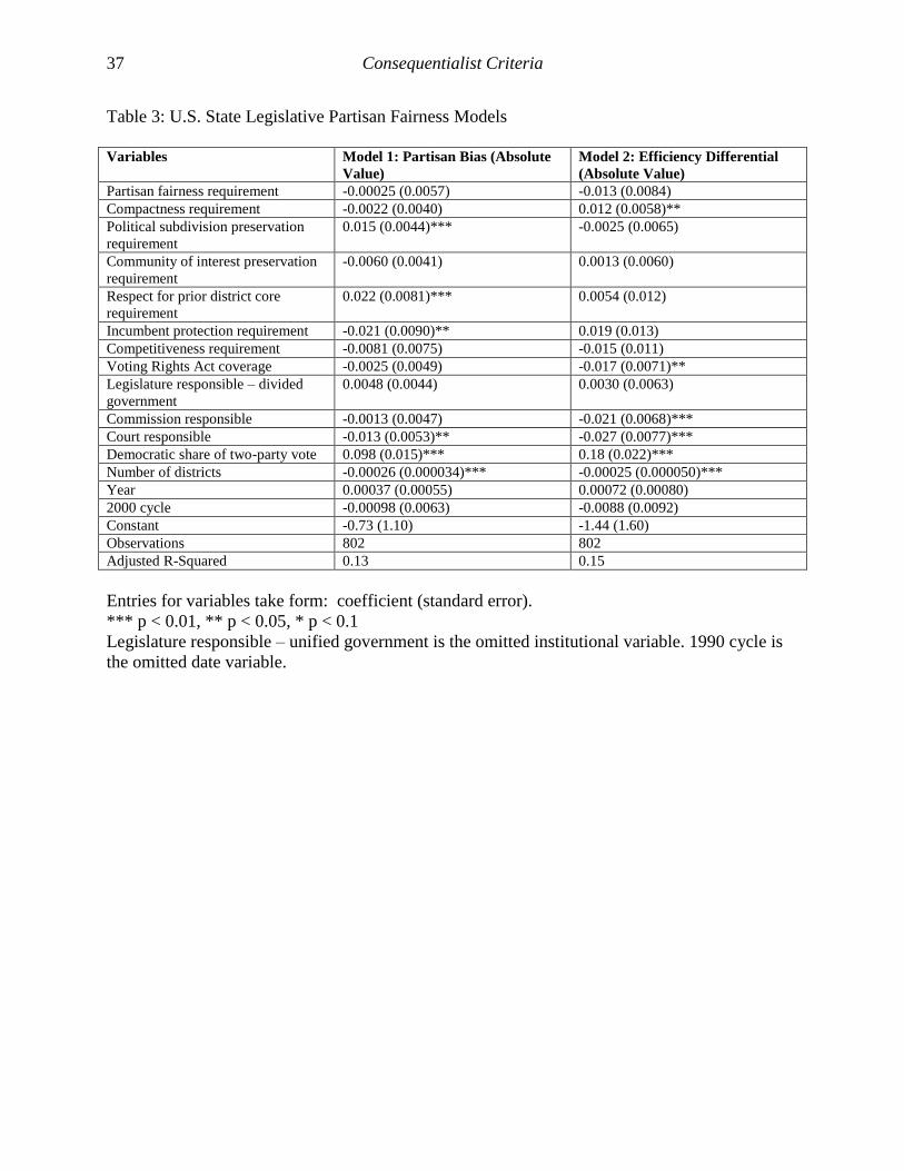
37 Consequentialist Criteria
Table 3: U.S. State Legislative Partisan Fairness Models
Variables Model 1: Partisan Bias (Absolute
Value)
Model 2: Efficiency Differential
(Absolute Value)
Partisan fairness requirement -0.00025 (0.0057) -0.013 (0.0084)
Compactness requirement -0.0022 (0.0040) 0.012 (0.0058)**
Political subdivision preservation
requirement
0.015 (0.0044)*** -0.0025 (0.0065)
Community of interest preservation
requirement
-0.0060 (0.0041) 0.0013 (0.0060)
Respect for prior district core
requirement
0.022 (0.0081)*** 0.0054 (0.012)
Incumbent protection requirement -0.021 (0.0090)** 0.019 (0.013)
Competitiveness requirement -0.0081 (0.0075) -0.015 (0.011)
Voting Rights Act coverage -0.0025 (0.0049) -0.017 (0.0071)**
Legislature responsible – divided
government
0.0048 (0.0044) 0.0030 (0.0063)
Commission responsible -0.0013 (0.0047) -0.021 (0.0068)***
Court responsible -0.013 (0.0053)** -0.027 (0.0077)***
Democratic share of two-party vote 0.098 (0.015)*** 0.18 (0.022)***
Number of districts -0.00026 (0.000034)*** -0.00025 (0.000050)***
Year 0.00037 (0.00055) 0.00072 (0.00080)
2000 cycle -0.00098 (0.0063) -0.0088 (0.0092)
Constant -0.73 (1.10) -1.44 (1.60)
Observations 802 802
Adjusted R-Squared 0.13 0.15
Entries for variables take form: coefficient (standard error).
*** p < 0.01, ** p < 0.05, * p < 0.1
Legislature responsible – unified government is the omitted institutional variable. 1990 cycle is
the omitted date variable.
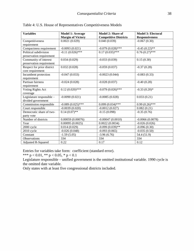
Consequentialist Criteria 38
Table 4: U.S. House of Representatives Competitiveness Models
Variables Model 1: Average
Margin of Victory
Model 2: Share of
Competitive Districts
Model 3: Electoral
Responsiveness
Competitiveness
requirement
0.0021 (0.029) 0.040 (0.039) -0.067 (0.30)
Compactness requirement -0.0093 (0.021) -0.079 (0.028)*** -0.45 (0.22)**
Political subdivision
preservation requirement
-0.11 (0.026)*** 0.17 (0.035)*** 0.76 (0.27)***
Community of interest
preservation requirement
0.034 (0.029) -0.033 (0.039) 0.15 (0.30)
Respect for prior district
core requirement
0.032 (0.028) -0.059 (0.037) -0.37 (0.28)
Incumbent protection
requirement
-0.047 (0.033) -0.0023 (0.044) -0.083 (0.33)
Partisan fairness
requirement
-0.024 (0.028) -0.028 (0.037) -0.40 (0.28)
Voting Rights Act
coverage
0.12 (0.020)*** -0.079 (0.026)*** -0.33 (0.20)*
Legislature responsible –
divided government
-0.0090 (0.021) -0.0085 (0.028) 0.033 (0.21)
Commission responsible -0.089 (0.025)*** 0.099 (0.034)*** 0.99 (0.26)***
Court responsible -0.0039 (0.020) -0.0012 (0.027) 0.082 (0.21)
Democratic share of two-
party vote
0.14 (0.07)** -0.15 (0.098) -0.35 (0.76)
Number of districts 0.00059 (0.00076) -0.00047 (0.0010) -0.0066 (0.0078)
Year 0.00095 (0.0025) 0.0022 (0.0034) -0.026 (0.026)
2000 cycle 0.014 (0.029) -0.099 (0.039)** -0.096 (0.30)
2010 cycle -0.026 (0.048) -0.093 (0.065) -0.035 (0.50)
Constant -1.59 (5.05) -3.96 (6.76) 54.4 (51.9)
Observations 334 334 334
Adjusted R-Squared 0.22 0.17 0.12
Entries for variables take form: coefficient (standard error).
*** p < 0.01, ** p < 0.05, * p < 0.1
Legislature responsible – unified government is the omitted institutional variable. 1990 cycle is
the omitted date variable.
Only states with at least five congressional districts included.
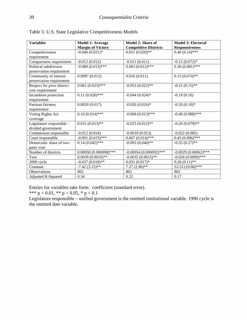
39 Consequentialist Criteria
Table 5: U.S. State Legislative Competitiveness Models
Variables Model 1: Average
Margin of Victory
Model 2: Share of
Competitive Districts
Model 3: Electoral
Responsiveness
Competitiveness
requirement
-0.040 (0.021)* 0.051 (0.020)** 0.40 (0.14)***
Compactness requirement -0.012 (0.012) -0.011 (0.011) -0.12 (0.072)*
Political subdivision
preservation requirement
-0.080 (0.013)*** 0.063 (0.012)*** 0.30 (0.081)***
Community of interest
preservation requirement
0.0097 (0.012) 0.016 (0.011) 0.15 (0.074)**
Respect for prior district
core requirement
0.061 (0.023)*** -0.053 (0.022)** -0.31 (0.15)**
Incumbent protection
requirement
0.11 (0.026)*** -0.044 (0.024)* -0.19 (0.16)
Partisan fairness
requirement
0.0020 (0.017) -0.026 (0.016)* -0.20 (0.10)*
Voting Rights Act
coverage
0.10 (0.014)*** -0.069 (0.013)*** -0.40 (0.088)***
Legislature responsible –
divided government
0.031 (0.013)** -0.025 (0.012)** -0.20 (0.079)**
Commission responsible -0.012 (0.014) -0.0018 (0.013) -0.022 (0.085)
Court responsible -0.091 (0.015)*** 0.067 (0.014)*** 0.45 (0.096)***
Democratic share of two-
party vote
0.14 (0.042)*** -0.093 (0.040)** -0.55 (0.27)**
Number of districts 0.00058 (0.000098)*** -0.00054 (0.000092)*** -0.0029 (0.00062)***
Year 0.0039 (0.0016)** -0.0035 (0.0015)** -0.026 (0.0099)***
2000 cycle -0.037 (0.018)** 0.031 (0.017)* 0.26 (0.11)**
Constant -7.42 (3.15)** 7.27 (2.96)** 53.53 (19.86)***
Observations 802 802 802
Adjusted R-Squared 0.34 0.22 0.17
Entries for variables take form: coefficient (standard error).
*** p < 0.01, ** p < 0.05, * p < 0.1
Legislature responsible – unified government is the omitted institutional variable. 1990 cycle is
the omitted date variable.