Embed Size (px)
Citation preview

Institutionen för Ekonomi,
Statistik och Informatik
The Capital Asset Pricing Model
Test of the model on the Warsaw Stock Exchange
C –Thesis
Author: Bartosz Czekierda
Writing tutor: Håkan Persson

The Capital Asset Pricing Model: Test of the model on the Warsaw Stock Exchange
2
Lucy: “I’ve just come up with the perfect
theory. It’s my theory that Beethoven would
have written even better music if he had been
married”
Schroeder: “What’s so perfect about that
theory?”
Lucy: “It can’t be proven one way or the other”
- Charles Schulz, Peanuts, 1976

The Capital Asset Pricing Model: Test of the model on the Warsaw Stock Exchange
3
Abstract
Since 1994 when the Warsaw Stock Exchange has been acknowledged as a full
member of World Federation of Exchanges and became one of the fastest
developing security markets in the region, it has been hard to find any studies
relating to the assets price performance on this exchange. That is why I decided
to write this paper in which the Nobel price winning theory namely the Capital
Asset Pricing Model has been tested.
The Capital Asset Pricing Model (or CAPM) is an equilibrium model which
relates asset’s risk measured by beta to its returns. It states that in a
competitive market the expected rate of return on an asset varies in direct
proportion to its beta.
In this paper the performance of 100 stocks traded continuously on the main
market in the years 2002-2006 has been tested. I have performed three
independent tests of the CAPM based on different methods and techniques to
better check the validity of the theory and then compared the results.
As in the case of many other studies of the Capital Asset Pricing Model, this one
didn’t find a complete support for the model but couldn’t reject some of its
features either.

The Capital Asset Pricing Model: Test of the model on the Warsaw Stock Exchange
4
Table of Content:
1. INTRODUCTION ......................................................................................................................... 6
1.1 Concept of the stock exchange ............................................................................................................... 6
1.2 Purpose of the study .............................................................................................................................. 6
1.3 The Warsaw Stock Exchange .................................................................................................................. 7
2. THEORETICAL BACKGROUND ................................................................................................ 9
2.1 Fundamental Share Price ........................................................................................................................ 9
2.2 Modern Portfolio Theory ...................................................................................................................... 10
2.1 The Capital Asset Pricing Model ........................................................................................................... 14
2.1 Theory of The Efficient Capital Market ................................................................................................. 17
3. PREVIOUS EMPIRICAL STUDIES OF THE CAPITAL ASSET PRICING MODEL ................ 18
4. METHODOLOGY ....................................................................................................................... 19
4.1 Data Selection ...................................................................................................................................... 19
4.2 Testable version of the CAPM .............................................................................................................. 20
4.1 Statistical Framework for Testing the CAPM......................................................................................... 21
4.3.1 The two-pass regression Test ............................................................................................. 21
4.3.2 Black, Jensen and Scholes Test ........................................................................................... 23
4.3.3 Black, Jensen and Scholes, Fama and MacBeth Test ..................................................... 24
4.1 Evaluating the Regression Results ........................................................................................................ 25
5.EMPIRICAL ANALYSIS ............................................................................................................. 26
5.1 The Two-Pass Regression Test .............................................................................................................. 26
5.1.1 SML Estimation ...................................................................................................................... 27
5.1.2 Non-Linearity Test ................................................................................................................. 28
5.1.3 Non-Systematic Risk Test ..................................................................................................... 29
5.2 Black, Jensen and Scholes Test ............................................................................................................. 29
5.2.1 SML Estimation ...................................................................................................................... 33
5.2.2 Non-Linearity Test ................................................................................................................. 34
5.2.3 Non-Systematic Risk Test ..................................................................................................... 34
5.3 Black, Jensen and Scholes, Fama and MacBeth Test ............................................................................. 34
5.3.1 SML Estimation ...................................................................................................................... 36

The Capital Asset Pricing Model: Test of the model on the Warsaw Stock Exchange
5
5.3.2 Non-Linearity Test ................................................................................................................. 37
5.3.3 Non-Systematic Risk Test ..................................................................................................... 37
6. SUMMARY AND CONCLUSIONS ............................................................................................ 39
6.1 Summary .............................................................................................................................................. 39
6.2 Conclusions and ideas for future studies .............................................................................................. 39
7. REFERENCES ........................................................................................................................... 41
APPENDIXES ................................................................................................................................ 42
Appendix A ................................................................................................................................................ 42
Table A................................................................................................................................................. 42
Table B ................................................................................................................................................ 44
Appendix B ................................................................................................................................................. 47
Table A................................................................................................................................................. 47
Table B ................................................................................................................................................ 49
Table C ................................................................................................................................................. 51
Table D ............................................................................................................................................... 54
Appendix C ................................................................................................................................................. 55
Table A................................................................................................................................................. 55
Table B ................................................................................................................................................ 57

The Capital Asset Pricing Model: Test of the model on the Warsaw Stock Exchange
6
1. Introduction
…When the first primitive man decided to use a bone for a club instead of eating its marrow, that was
investment.
-Anonymous
1.1 Concept of the stock exchange1
The main idea of the stock exchange is to provide firms with capital and equity. They do so by issuing
common stocks which can be purchased and traded on the market. Price of such a stock is usually
defined as a net present value of company’s future cash flows. If a person owns a share he’s entitled
to a fraction of the firm’s profit and essentially owns a part of the firm. Stock exchanges are usually
organized to separate new stock issues from daily trading. If a company wishes to raise additional
funds for new capital by issuing new shares it does this on the primary market while existing shares
are traded on the secondary market. There are two main types of exchanges: auction markets and
dealer markets. On the auction market, which is definitely the most popular type, an auctioneer
works as an intermediary and matches potential buyers and sellers. The dealer market is
characterized by the presence of dealer groups which trade with the investors directly. Dealer
markets are not particularly popular for stock trading but other financial instruments such as bonds
are usually traded that way.
1.2 Purpose of the study The main objective of this paper is to check the validity of the Capital Asset Pricing Model using the
assets traded on the Warsaw Stock Exchange. The Capital Asset Pricing model or in short the CAPM is
equilibrium model that relates stocks risk measured by beta to their returns. Its main massage is that
stocks returns are increasing proportionally to their betas and that this relationship is positive and
linear. It is expressed by so called Security Market Line. A complete derivation and logic behind the
model will be described in Chapter 2. The testing procedure will be concentrated on properties of
this Security Market Line using the ordinary least squares and multiple regressions as main analytical
tool. In this paper three independent tests of the model will be performed based on previous studies
of the researchers such as Black, Jensen, Scholes, Fama and MacBeth2. Chapter 3 will describe their
studies in more detail. I will use the monthly returns on the stocks in the years 2002-2006. Due to
this relatively short testing period the original tests must be modified to accommodate the available
data. This process will be described in Chapter 4 followed by the empirical analysis in Chapter 5 and
the conclusions in Chapter 6.
1 Brealey, Myers, Allen [2006] p.60-61 2 Haugen Robert A. [2001] p.238-139
The Capital Asset Pricing Model: Test of the model on the Warsaw Stock Exchange
7
1.3 The Warsaw Stock Exchange3 The origins of Polish financial markets date back to the 19th century. On May 12, 1817 the first stock
exchange known as the Mercantile Exchange was founded in Warsaw. Financial instruments traded
in that time were primarily bonds and bills of exchange. Assets similar to stocks developed during the
second half of the 19th century. The Warsaw exchange was not the only market operating in Poland
at that time. Similar exchanges were founded in Katowice, Krakow, Lvov, Lodz, Poznan and Vilnius. By
1939 there were 130 securities traded on the exchange including municipal, corporate and
government bonds as well as shares.
Unfortunately further development of the financial sector was interrupted by historical events.
World War II and later the operation of the communistic system put a stop to trading for many years.
After the fall of the regime a need for a well functioning financial system arose again. In 1990 Poland
signed an intergovernmental agreement with France to create a new stock exchange in Warsaw. Not
long afterwards in 1991 the Warsaw Stock Exchange (WSE) was officially opened. It took 3 more
years however until WSE could be accepted as a full member of World Federation of Exchanges.
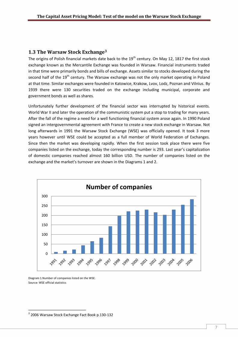
Since then the market was developing rapidly. When the first session took place there were five
companies listed on the exchange, today the corresponding number is 293. Last year’s capitalization
of domestic companies reached almost 160 billion USD. The number of companies listed on the
exchange and the market’s turnover are shown in the Diagrams 1 and 2.
Diagram 1.Number of companies listed on the WSE.
Source: WSE official statistics
3 2006 Warsaw Stock Exchange Fact Book p.130-132
0
50
100
150
200
250
300
Number of companies

The Capital Asset Pricing Model: Test of the model on the Warsaw Stock Exchange
8
Diagram 2.Share turnover on WSE in mln PLN (1 USD 2,8 PLN)
Source: WSE official statistics
The Warsaw Stock exchange is a joint stock company with almost 60 000 shares outstanding. In 2005
it had 38 shareholders including brokerage houses, banks, and the State Treasury which holds 98, 81
% of all shares. The objectives of the WSE are stated in its mission and vision.
Mission of the WSE4
- To provide a transparent, effective and liquid market that concentrates trading in Polish financial instruments;
- To provide the highest quality of service to Polish market participants ; - To provide a capital allocation and mechanism to finance the Polish economy; - To foster capital markets’ development in Poland.
The WSE's Vision5
- To achieve a 50% market capitalization/GDP ratio; - To maintain the leading position on the domestic capital market; - To become the largest exchange in the region and an important hub in the network of
European exchanges.
Trading on WSE is organized into two main markets:
- Main market (official quotations)
- Parallel market
Assets traded on the main market belong to the companies with the largest liquidity which usually
have a longer history while companies listed on the parallel market are smaller, younger and have
less capital.
4 2006 Warsaw Stock Exchange Fact Book p.7-8 5 2006 Warsaw Stock Exchange Fact Book p.7-8
050000
100000150000200000250000300000350000400000
1991
1992
1993
1994
1995
1996
1997
1998
1999
2000
2001
2002
2003
2004
2005
2006
Turnover from shares

The Capital Asset Pricing Model: Test of the model on the Warsaw Stock Exchange
9
2. Theoretical background
In this section all the necessary theory of the stock valuation and portfolio management will be
presented. I will start with the concept of asset valuation referred to as the fundamental share price.
Next step will be to describe the modern portfolio theory created by Harry Markowitz and the theory
of his followers Sharpe and Lintner known as Capital Asset Pricing Model (CAPM).Finally I will mention
the theory of efficient capital markets.
2.1 Fundamental share price6 Fundamental share price is the most basic concept of the firm’s valuation. It states that the market
value of the share is the discounted value of all future expected cash flows from the company to its
owners. The underlying assumption is that company desires to maximize the wealth of its
stockholders which is equivalent to maximizing the value of the outstanding shares. Microeconomic
theory assumes the profit maximization model of the company but fortunately the profit
maximization and the shareholders’ wealth maximization are goals very similar to each other.
Assume that shares price is in period t. If a company pays out a dividend and the expected
value of the share in the period t+1 is then the stockholders expected gain from holding a share
is - . If prevailing interest rates on risk-free asset is r and the risk-premium for
normally risk-averse investors is ε then the equilibrium condition on the market reads:
(1)
Solving this equation for gives the first expression for the stock price as a discounted value of the
expected dividend and the expected price:
(2)
Using this equation one can obviously express the stock price for any period of time: ,
,…. . Substituting expressions for future prices into equation 2 gives:
(3)
If we assume that investors do not expect stock prices to rise indefinitely at rate faster than
(if that was the case the price today would by infinitely high), then we conclude that
and equation 3 can be rewritten as follows:
(4)
The expression above is known as the fundamental share price and as mentioned it is equal to the
present value of expected cash flows i.e. dividends to the shareholders. In order to pay out dividends
a company must earn a positive profit so the owners’ wealth maximization means firms profit
maximization.
6 Sørensen Peter Birch, Whitta-Jacobsen Hans Jørgen [2005]” p. 337-339
The Capital Asset Pricing Model: Test of the model on the Warsaw Stock Exchange
10
2.2 Modern portfolio theory7 Modern portfolio theory is a set of concepts created by Harry Markowitz8 in the early fifties. He
introduced a measurement of assets risk and developed methods for combining them into risk-
efficient portfolios, thus creating an important base for further evolution of financial theory.
The two most important values of any asset are its returns over time and the volatility of these
returns. Measured over some fairly short interval of time, the rates of returns conform closely to
normal distribution, while studying longer periods of time exhibits the distribution that could be
described as lognormal i.e. skewed to the right9 10. However it is commonly assumed that rates of
returns are distributed normally. To describe such a distribution we need only two numbers: mean
and standard deviation. Translating into financial definitions, mean describes expected return of the
asset and standard deviation is a measurement of the risk. Risk and return are the only things that
investors pay attention to while making their investment decisions.
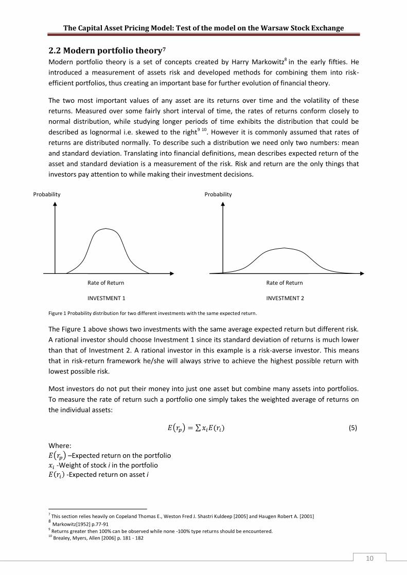
Figure 1 Probability distribution for two different investments with the same expected return.
The Figure 1 above shows two investments with the same average expected return but different risk.
A rational investor should choose Investment 1 since its standard deviation of returns is much lower
than that of Investment 2. A rational investor in this example is a risk-averse investor. This means
that in risk-return framework he/she will always strive to achieve the highest possible return with
lowest possible risk.
Most investors do not put their money into just one asset but combine many assets into portfolios.
To measure the rate of return such a portfolio one simply takes the weighted average of returns on
the individual assets:
(5)
Where:
–Expected return on the portfolio
-Weight of stock i in the portfolio -Expected return on asset i
7 This section relies heavily on Copeland Thomas E., Weston Fred J. Shastri Kuldeep [2005] and Haugen Robert A. [2001]
8 Markowitz[1952] p.77-91 9 Returns greater then 100% can be observed while none -100% type returns should be encountered.
10 Brealey, Myers, Allen [2006] p. 181 - 182
Probability Probability
Rate of Return
INVESTMENT 1
Rate of Return
INVESTMENT 2

The Capital Asset Pricing Model: Test of the model on the Warsaw Stock Exchange
11
Calculating the risk of the portfolio is much trickier. Multiplying individual assets’ standard deviations
by their weights in the portfolio and summing them up could only work if all the securities in the
portfolio were perfectly correlated with each other. This is rarely the case.
In his studies Markowitz11 discovered that combining stocks into portfolios can substantially reduce
the standard deviation of portfolio, thus introducing the concept known as diversification.
Diversification is possible because prices of different stocks are not perfectly correlated with each
other. In the Figure 2 below we can see how the increasing number of assets in the portfolio reduces
its risk.
Figure 2 How diversification reduces risk. Source: Brealey, Myers, Allen [2006]
We can see that as an investor increases number of assets in his portfolio the overall risk diminishes.
It is also worth mentioning that the reduction of risk is most noticeable with only a few securities and
as we put more stocks into portfolio reduction becomes smaller and smaller and ceases at some
point. The risk that can be diversified is also called the unique risk while non avoidable risk is known
as the market risk.
Knowing how the standard deviation of the portfolio changes with an increasing number of
securities. It can by now shown how to calculate it. The simplest case is with just two assets and the
formula looks like the one below:
(6)
Where:
-Portfolio standard deviation -Weight of stock 2 in the portfolio
- Variance of stock -Weight of stock 1 in the portfolio
- Variance of stock 1 -Covariance between stocks 1 and 2
11 Markowitz[1952] p.77-91
Standard deviation
Number of securities
Market Risk
Unique Risk
The Capital Asset Pricing Model: Test of the model on the Warsaw Stock Exchange
12
A
MVP
Adding more stock into the portfolio involves putting more variables into the equation above,
especially covariances. For instance portfolio with 3 securities involves 3 terms for weighted
variances and 6 terms for weighted covariances12.
The next question that arises is how many of each stock an investor should have in his/her portfolio
to minimize the risk and maximize the expected return? To answer this question we must employ
equations 5 and 6 to calculate the expected rates of return and the standard deviations for different
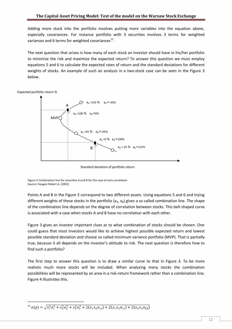
weights of stocks. An example of such an analysis in a two-stock case can be seen in the Figure 3
below.
Figure 3 Combination line for securities A and B for the case of zero correlation Source: Haugen Robert A. [2001]
Points A and B in the Figure 3 correspond to two different assets. Using equations 5 and 6 and trying
different weights of these stocks in the portfolio (xA, xB) gives a so called combination line. The shape
of the combination line depends on the degree of correlation between stocks. This bell-shaped curve
is associated with a case when stocks A and B have no correlation with each other.
Figure 3 gives an investor important clues as to what combination of stocks should be chosen. One
could guess that most investors would like to achieve highest possible expected return and lowest
possible standard deviation and choose so called minimum variance portfolio (MVP). That is partially
true, because it all depends on the investor’s attitude to risk. The next question is therefore how to
find such a portfolio?
The first step to answer this question is to draw a similar curve to that in Figure 3. To be more
realistic much more stocks will be included. When analyzing many stocks the combination
possibilities will be represented by an area in a risk-return framework rather than a combination line.
Figure 4 illustrates this.
12
B
Standard deviation of portfolio return
Expected portfolio return %
xA =100 % xB =0%
xA =45 % xB =-65%
xA =-25 % xB =125%
xA =0 % xB =100%
xA =150 % xB =-50%

The Capital Asset Pricing Model: Test of the model on the Warsaw Stock Exchange
13
MVP
A
B
Figure 4 Optimal choices of investment portfolio Source: Copeland Thomas E., Weston Fred J. Shastri Kuldeep [2005]
The diamond-like points in the figure above represent positions of single stocks in the risk-return
framework. The shaded area represents so called the feasible set and it contains all the portfolios
that can be constructed from these individual securities. When choosing a portfolio investors want to
achieve the highest expected return possible according to their risk preferences. However no rational
investor would invest in a portfolio below the minimum variance portfolio (MVP) since higher return
can be achieved with the same risk. The part of the feasible set market with the red curve is called
the efficient frontier because it contains portfolios defined by Markowitz as efficient portfolios. The
main feature of these portfolios is that they offer the best possible expected return given a certain
amount of risk.
Now it is possible for us to see which portfolios will be chosen. According to common practice in
microeconomics the investors’ preferences will be marked with utility functions represented by
indifference curves I-III. An investor with indifference curve III is definitely a risk loving one since he
chooses portfolio A with high return and high risk. An investor with indifference curve II can tolerate
some risk thus chooses portfolio B while investor with utility function I is most the risk averse of
them all and chooses minimum variance portfolio.
Knowing where the price of the stock comes from, how diversification reduces risk and how investors
make their investment decisions by choosing efficient portfolios it is now possible to derive an
extension of Markowitz’s modern portfolio theory: the capital asset pricing model.
Standard deviation of portfolio return
Expected portfolio return %
III II
I

The Capital Asset Pricing Model: Test of the model on the Warsaw Stock Exchange
14
Standard deviation
Efficient frontier
CML
rf
M
A
B
(RM)
E(RM)
C
D
2.3 The Capital Asset Pricing Model (CAPM)13 The capital asset pricing model was created approximately 10 years after Markowitz’s14 famous
article. The model was developed almost simultaneously by four researchers: Sharpe, Treynor,
Mossin and Linter. In short the CAPM is a theory about how assets’ price is related to their risk15.
Before I can proceed and derive the model, a couple of assumptions must be made about investors
and assets. I will use the same assumptions as Copeland, Weston and Shastri used in their handbook
“Financial Theory and Corporate Policy”:
- Assumption 1: Investors are risk-averse individuals who maximize the expected utility of
their wealth
- Assumption 2: Investors are price-takers and have homogenous expectations about asset
returns that have a joint normal distribution.
- Assumption 3: There exists a risk-free asset such that investors may borrow or lend unlimited
amounts at the risk-free rate.
- Assumption 4: The quantities of assets are fixed. Also, all the assets are marketable and
perfectly divisible.
- Assumption 5: Asset markets are frictionless, and information is costless and simultaneously
available to all investors.
- Assumption 6: There are no market imperfections such as taxes, regulations, or restrictions
on short selling.
One additional assumption should be made that all investors follow the Markowitz’s portfolio
selection theory and choose efficient portfolios.
Let’s start the derivation of CAPM by incorporating the risk-free interest rate assumption. A risk-free
interest rate is defined as rate of return on investment with standard deviation equal to 0. In
practical situations returns on assets such as government bonds are assumed to be risk-free
Figure 5 Derivation of Capital Market Line
13 This section relies heavily on Copeland Thomas E., Weston Fred J. Shastri Kuldeep [2005] and Haugen Robert A. [2001] 14 Markowitz[1952] p.77-91 15
Copeland Thomas E., Weston Fred J. Shastri Kuldeep [2005]
Expected return %

The Capital Asset Pricing Model: Test of the model on the Warsaw Stock Exchange
15
Consider Figure 5 above. It represents a well known risk-return framework. From the whole feasible
set only the efficient frontier has been drawn. Assume now that this efficient frontier was derived
from a set containing all the securities available on the market. With a presence of the risk-free asset
the efficient frontier becomes linear and is called the Capital Market Line. The Capital Market Line
(CML) can be written mathematically and its formula is:
(7)
Where:
- Expected return
-Expected return on market portfolio
-Risk-free rate of return
-Risk of market portfolio
-Risk measured by standard deviation
Note that CML is tangent to the “old” efficient frontier in point M. Moving along the CML from point
up to point M an investor is lending some of his money and investing the rest in portfolio M,
whereas moving from point M and to the right means that the investor is borrowing funds in order to
invest his own money and the loan in portfolio M. Point M represents a market portfolio16 and if
investors are rational they will only choose a combination of risk-free asset and this portfolio,
depending on their risk preferences. Consider point A for instance which is a minimum variance
portfolio, an investor will be clearly better off by investing in portfolio C containing a mixture of risk-
free and risky assets. The situation is the same in the case of point B where a better alternative is to
borrow some money at and invest more in the market portfolio achieving point D.
After introducing a risk-free interest rate into the portfolio creation process we know what
combination of market portfolio and risk-free assets is appropriate for different investors. In the end
all investors are concerned about is the final position of their investments in the risk-return
framework. For this reason it is plausible to assume that investors will assess the risk of an individual
security on the basis of its contribution to the risk of the portfolio17. A measurement of such a risk
contribution is known as beta and it’s defined as18:
(8)
Where:
- Covariance between the market portfolio and a single asset
- Variance of the market portfolio return
16 As mentioned the efficient front was derived from a feasible set containing all securities available on the market. 17 Haugen Robert A. [2001] p.209 18 Beta can also be calculated from a linear regression by regressing return on the market as the independent variable and return on the asset as the dependent one. The result should be the same.

The Capital Asset Pricing Model: Test of the model on the Warsaw Stock Exchange
16
rf
ri)
1 0
M
rM) - rf
SML
rM)
Beta can also be interpreted the other way around i.e. how sensitive an individual asset is to the
market movements. By definition market portfolio (such as M in Fig.5) has a beta = 1. If a stock has a
beta coefficient equal 0, 5 it means that it amplifies half of the market movements. We call such a
stock a “defensive” one. If on the other hand stock’s beta is greater then 1, it tends to react much
stronger than the market. We call such a stock an “aggressive” one.
We now have a new definition of risk defined by beta so Figure 5 should be modified to represent
this change. The risk-free asset will be unaffected since its risk is always 0. As mentioned market
portfolio will have beta equal to one. Having these two points we can now draw a new figure with
beta as a measure of risk.
Figure 6 The Capital Asset Pricing Model Source: Haugen Robert A. [2001]
Figure 6 presents the capital asset pricing model in a whole glance. Standard deviation has been
replaced by beta and the line that was previously the capital market line is called security market line
(SML) in this framework. Note that market portfolio M is exactly the same as in Figure 5. We can
write the SML’s equation now by taking values directly from the Figure 5 above:
(9)
Where:
-Expected rate of return on an asset or a portfolio
- Risk-free rate of return
-Expected return on market portfolio
-Beta coefficient of an asset or a portfolio
We can rearrange it to express it in terms of an expected excess of returns on an asset or portfolio
over the risk –free return:
(10)
The Capital Asset Pricing Model: Test of the model on the Warsaw Stock Exchange
17
Where:
This excess is also defined as a risk premium which is demanded by investors for bearing additional
risk. According to the model this premium should be proportional to the stock’s beta so in
equilibrium all the assets should lie on the SML19. If a stock was lying above the security market line it
would offer greater return with the given beta than predicted in equilibrium. Investors would rush to
buy it thus pushing up the price and lowering the return so the stock would eventually end up on the
line. If the stock was below the SML the opposite would happen. There would be other assets
offering greater return with the same risk so investors would sell out the asset undercutting the price
thus increasing its return.
Assuming that CAPM is true it provides two important clues about the strategy of investing20:
- Diversify your portfolio of risky assets in proportion to market portfolio
- Mix your risky assets with risk-free securities to achieve the desired level of risk
2.4 Theory of the efficient capital market Another very important contribution to the knowledge of financial markets is so called Efficient
Market Hypothesis. A base for the theory was the discovery made by Maurice Kendall21 in 1953 who
studied prices of financial instruments and commodities. He found out that there is no pattern in
behavior of these prices and described the phenomenon as the random walk22. It means that
studying the past prices cannot help investors to predict what will happen in the future. In the late
1970: s Fama formed three types of market efficiency based on Kendall’s discovery23:
- Weak-form efficiency: no extra profits can be made by studying historical prices. In other
words present prices already reflect all the information that can be gained from past prices.
- Semi-strong-form efficiency: no extra profits can be made by interpreting publicly available
information. The prices already reflect all published information.
- Strong-form efficiency: no extra profits can be made by using any information whether it is
public or not because prices already reflect all possible information.
The idea that stock prices are unpredictable and move without any clear pattern will be used later in
the paper in order to modify the Capital Asset Pricing Model so it can be tested using historical
returns.
19 Brealey, Myers, Allen [2006] p.189 20
Bodie Ziv , Merton Robert C. [2000] 21
Brealey, Myers, Allen [2006] p.189 22
Brealey, Myers, Allen [2006] p.333-337 23
Copeland Thomas E., Weston Fred J. Shastri Kuldeep [2005] p.354-355
The Capital Asset Pricing Model: Test of the model on the Warsaw Stock Exchange
18
3. Previous empirical studies of the Capital Asset Pricing Model
Since the CAPM was established a number of empirical studies have been performed to test the
model in reality. The results of these studies were very different: some tests supported the CAPM
hypothesis; some of them rejected it completely.
The first supportive empirical study of the CAPM was published in 1972 by three researchers Black,
Jensen and Scholes24. Their research concentrated on the properties of the security market line in the
model and used the technique known as the cross-section test for the first time. As the population
they chose all stocks listed on the New York Stock Exchange in years 1926 – 1965. First stock betas
were estimated by regressing stocks’ monthly returns during the first four years with monthly
returns of the market index. In the next step they created 10 portfolios based on stocks’ estimated
betas25 and computed monthly returns on these portfolios during the fifth year. This procedure was
repeated until the end of the testing period. Finally they estimated portfolio betas and related them
to their average returns, getting an approximation of the security market line. The results of their
test were very promising and supportive for the CAPM. The relationship between portfolios betas
and their average returns was linear with a positive and significant slope. Similar conclusion can be
found in a later study of CAPM published by Fama and MacBeth26 in 1974. They used a similar
technique to Black, Jensen and Sholes with one major distinction: they tried to predict future rates of
return based on estimates from previous periods. Nevertheless results were again supportive.
The capital asset pricing model has been criticized on several occasions. In the late 1970’s Richard
Roll27 wrote several papers in which he criticizes the model and its assumptions. He argues that the
model could only be tested by testing if the market portfolio is efficient and since it should contain all
the financial instruments on the international market it is impossible to test it. Another study
performed by Fama and French28 in 1992 as an extension of the Fama and MacBeth experiment from
1974 showed a couple of anomalies that couldn’t be explained by the CAPM. They looked beyond the
returns and took company size under consideration. According to their study it would seem that on
average small companies tend to have larger rates of return which is inconsistent with CAPM where
only beta can influence the returns. Other studies have discovered that there are more factors that
could also explain rates of return not predicted by the Capital Asset Pricing Model.
Reinganum in 1983 argued that in January risk premiums tend to be higher while French in 1980
stated that on Mondays same premiums are on average lower. Other studies showed that
earnings/price ratio as well as book-to-market value has positive influence on risk premiums29.
Despite all the critique the CAPM is widely used in the industry. It is used to help making capital
budgeting decisions or measuring the performance of investment managers and is also a very useful
benchmark.
Ddd
24
Haugen Robert A. [2001] p.238 25
10% of stocks with highest betas formed one portfolio, 10% of next highest betas formed next portfolio etc. 26
Haugen Robert A. [2001] p.239 27
Copeland Thomas E., Weston Fred J. Shastri Kuldeep [2005] p.242 28
Haugen Robert A. [2001] p.240 29
Grigoris Michailidis, Stavros Tsopoglou, Demetrios Papanastasiou, Eleni Mariola [2006]

The Capital Asset Pricing Model: Test of the model on the Warsaw Stock Exchange
19
4. Methodology
In this section I will present the methods on which the empirical analysis will be based. First I will
discuss the data source and data selection process. Next I will modify the model and make certain
assumptions to make the results more reliable. Finally I will describe the statistical methods that will
be used for testing the CAPM.
4.1 Data Selection To test the Capital Asset Pricing Model data from official statistics of the Warsaw Stock Exchange will
be used. The exchange has existed since 1994 but access to reliable data is provided from the year
2002. That is the main reason why this study will be conducted by analyzing monthly returns on
common stocks from 2002 to 2006.
In this paper one hundred companies listed without any interruptions will be analyzed. I decided to
divide the population in half and randomly choose 50 companies defined as big capitals and 50
companies defined as small capitals to cover the market as a whole. A NASDAQ definition of big
capital states that it is a company with more than $5 billion in capitalization30. Since Polish companies
cannot be compared to those in USA the definition has to be modified. After analyzing the data it
seemed plausible to define a big capital on the Polish market as a company with a capitalization of
more than PLN 585 million (around $1, 6 billion)31. The main reason why I decided to divide
population by the size not by the branch is that it has been observed that size of company has certain
influence on its stock returns. On the other hand it hasn’t been proven that companies in certain
industries have a tendency to over- or underperform the market.
As the representation of the market I choose market index WIG which contains 284 companies out of
293 listed on whole exchange. Other indexes available are WIG20 listing 20 biggest companies,
mWIG40 containing 40 medium firms, sWIG80 with 80 small capitals. There are also a couple indexes
strongly connected to certain branches. Out of all these indexes only WIG seems to be the best proxy
of a market as a whole.
The last data set needed to perform the test is the interest rate on the risk-free asset. As a proxy of
that rate I choose the rate of return on a 52 week government bond issued by the Polish Central
Bank. This rate has been converted into monthly rate by simply dividing it by 12 each month. The
development of the risk-free interest rate over the testing period can be seen in the Figure 8 below.
30
http://www.investorwords.com/2722/large_cap.html 31
The whole population was sorted by companies’ capitalization rate and then divided into two groups. The border value was used to
define large and small capital.

The Capital Asset Pricing Model: Test of the model on the Warsaw Stock Exchange
20
Figure 7 Development of the risk-free rate of return Source: Polish Central Bank: www.nbp.pl
4.2 Testable version of the CAPM In section 2.3 the CAPM was derived in two versions which will be rewritten here for convenience.
The most common version of CAPM is:
(11)
(12)
The second version of CAPM expresses the returns in terms of their excess over the risk-free rate and
it can be written as follows32:
(13)
(14)
The problem might arise because betas are not calculated from the same values in these two
versions, thus they can differ. However if the risk-free rate is non-stochastic equations 12 and 14 are
equivalent33. Proxies of the risk-free rates in the real world might happen to be stochastic. The
distribution of the risk-free rate used in this study can be seen in Figure 7. Regardless if the risk-free
rate is stochastic or not most of the empirical work on CAPM employs excess returns version34, thus
this paper will also employ the CAPM based on equations 13 and 14.
32
Remember: , 33
Campbell John Y., Lo Andrwe W., MacKinlay Craig A. [1997] p.182 34 Campbell John Y., Lo Andrwe W., MacKinlay Craig A. [1997] p.182
0,00%
2,00%
4,00%
6,00%
8,00%
10,00%
12,00%
apr-01 sep-02 jan-04 maj-05 okt-06 feb-08
Rat
e o
f R
etu
rn
Time
Development of the risk-free rate of return. Years 2002-2006
52 week rate
4 week rate

The Capital Asset Pricing Model: Test of the model on the Warsaw Stock Exchange
21
The next important step to prepare the CAPM for empirical testing is to transform it from
expectations form (ex ante) into ex post form which uses the actual observed data. To do so an
employment of efficient market hypothesis will be used, known as a fair-game model. A fair game
model states that on average, studying a large number of samples, the expected return on an asset
equals its actual return35. Mathematically it can be expressed as follows:
(15)
(16)
Where:
– The difference between actual and expected returns
- Actual return
- Expected return
Equation 15 is quite straightforward while equation 16 states that the expected value of the
difference between the actual and expected returns is 0. We are simply assuming that probability
distributions of returns do no change significantly over time36.
Removing expectations terms from the equation 13 reveals the CAPM that will be tested in this
paper:
(17)
4.3 Statistical framework for testing the CAPM
I decided to run three independent tests of the CAPM using different techniques and then compare
the results with each other. The first test is based on one of the earliest attempts to check the
validity of the theory which uses so a called two-pass regression technique. The second test will be
based on Black, Jensen, and Sholes37 (BJS) research from 1972 and will employ a cross-sectional
analysis of the assets. Finally I will use combined ideas of BJS studies and Fama-MacBeth38 research
from 1974 that also uses a cross-sectional technique.
4.3.1 The two-pass regression test
The first step in testing the CAPM using this method is to use the monthly excess returns on 100
chosen assets over the testing period 2002-2006 to estimate their betas. To do it a time series OSL
regression will be run for every single asset (First-pass regression). The regression equation will be:
(18)
35
Copeland Thomas E., Weston Fred J. Shastri Kuldeep [2005] p.367 36
Haugen Robert A. [2001] p.236 37
Haugen Robert A. [2001] p.238 38
Haugen Robert A. [2001] p.239

The Capital Asset Pricing Model: Test of the model on the Warsaw Stock Exchange
22
Where:
- Excess of an asset’s returns over the risk free rate at time t
-Regressions intercept
- Estimated beta of asset i
- Excess of the market returns over the risk free rate at time t
- Random disturbance term at time t
In total 100 time-series regressions will be performed on this stage of analysis. According to CAPM
the intercept of the regression described by equation 18 should be 0, whereas there are no
restrictions on the value of beta. After estimating betas I will attempt to estimate the security
market line for the testing period. To do so a second-pass regression will be run according to the
equation:
(19)
Where:
- Average excess of returns on asset i over the testing period
- Regression intercept
- Regression coefficient
- Estimated beta of the asset i
- Random disturbance term.
This regression will be run across all one hundred assets resulting in an estimation of SML. If CAPM
holds the results should be as follows:
The next step will be to perform so called non-linearity test. As mentioned in the theoretical section
CAPM predicts that assets’ returns are linearly related to their betas. In order to test this hypothesis
an additional term will be added to equation 19:
(20)
Term is simply a second power of our estimated beta. If the model indeed holds and the linear
relationship between beta and returns is strong then adding the beta square term shouldn’t
influence the previous results. Thus if CAPM is true then:
The last check of the theory that can be performed is a test for non systematic risk. The CAPM says
that the only risk that matters to investors, which is reflected in returns, is measured by beta. Any
other factors simply don’t matter. To account for non systematic risk yet another parameter will be
added to the regression equation:
(21)

The Capital Asset Pricing Model: Test of the model on the Warsaw Stock Exchange
23
The term stands for the variance of residuals of an asset i. We obtain the value of this term from
the first-pass regression that has been used to estimate stocks betas. Residual variance in this case
will be the measure of the risk not accounted by beta. If CAPM holds then:
4.3.2 Black, Jensen and Scholes Test
The second test of the CAPM that I will perform is based on the Black, Jensen and Scholes test from
1972 which is described in more detail in section 3. Due to a much shorter testing period their
technique must be modified to accommodate available data. The BJS test studies the performance of
the CAPM on the portfolios rather than single stocks. By creating portfolios, a certain amount of
company-specific risk will be diversified in accordance with Markowitz’s modern portfolio theory.
The testing procedure will be performed in following steps:
1. Stocks’ betas will be estimated using equation 18 based on monthly returns in the years
2002-2003.
2. Stocks will be ranked by their estimated betas and 10 portfolios will be created based on
stocks’ betas; 10 % of the stocks with the lowest betas create the first portfolio and so on,
until 10 portfolios are created.
3. The monthly returns on these portfolios will be computed in the year 2004. A monthly return
on a portfolio is simply an arithmetic average of the monthly returns on the stocks in the
portfolio.
4. Stocks’ betas will be re-estimated using equation 18 based on monthly returns in years 2003-
2004.
5. The portfolios will be reconstructed using the same method described in step 2 and betas
from step 4. The monthly returns on the portfolios in year 2005 will be computed.
6. Stocks’ beta will be estimated one more time using equation 18 based on the monthly
returns in the years 2004-2005.
7. The portfolios will be reconstructed again and their returns will be computed for the year
2006.
8. The portfolios betas will be estimated by regressing returns computed in steps 3, 5 and 7 to
the market index. The regression equation is:
(22)
Where:
- Excess of the portfolio returns over the risk free rate at time t
-Regressions intercept
- Estimated beta of the portfolio p
- Excess of the market returns over the risk free rate at time t
- Random disturbance term at time t
The Capital Asset Pricing Model: Test of the model on the Warsaw Stock Exchange
24
9. The cross-sectional regression will be performed to estimate SML by regressing portfolios’
average excess of returns over the risk-free rate in 2004-2006 to their betas estimated in the
step 8. The regression equation is:
(23)
Where:
- Average excess of returns on portfolio p over the testing period
- Estimated beta of the portfolio p
- Random disturbance term.
10. The non-linearity and non-systematic risk tests will be performed according to the equations:
(24)
(25)
The logic behind equations 24 and 25 is exactly the same as in the first test using a two-pass
regression technique.
If the Capital Asset Pricing Model is true the values of regressions’ coefficients should equal to:
4.3.3 Black, Jensen and Scholes, Fama and MacBeth Test.
The last empirical test of the CAPM will be very similar to the BJS analysis performed earlier.
However this time I will incorporate some ideas used by Fama and MacBeth in their study from 1974.
Again portfolios are used to test the model, however this time the performance of 20 portfolios will
be tested. Moreover the portfolios will be constructed only once so they will have the same content
during the whole testing period. The testing procedure will be performed in the following steps:
1. Stocks’ betas will be estimated using equation 18 based on monthly excess of returns in the
years 2002-2003.
2. Stocks will be ranked by their estimated betas and 20 portfolios will be created based on
stocks’ betas; 5 % of stocks with the lowest betas will create the first portfolio and so on until
20 portfolios are created.
3. The monthly excess returns on these portfolios will be computed in the years 2003-2005 as
the arithmetic average of monthly excess returns on the stocks in the portfolio.
4. Portfolios’ betas will be estimated using equation 22 by regressing their monthly excess
returns in the years 2003-2005 against the market index.

The Capital Asset Pricing Model: Test of the model on the Warsaw Stock Exchange
25
5. The cross-sectional regression will be performed according to equation 23 to estimate SML
by regressing portfolios’ average excess of returns in the year 2006 to their betas estimated
in step 4.
6. Non-linearity and the non-systematic risk test will be performed utilizing equations 24 and
25.
If the CAPM holds the cross-sectional regression results should be:
4.4 Evaluating the regressions results
To evaluate the results obtained by performing the regressions I will use the t- test and p-value
criterion. During the empirical analysis the t-value statistic will be given for every important estimate.
The critical values for the t-statistic are -1, 96 and 1, 96 which means that if the t-value is greater
than 1, 96 or smaller than -1, 96 the results are statistically significant with 95% confidence i.e. the
probability of receiving a certain result is 95 %. When analyzing final Security Market Line
Estimations, the p-value will be given for every parameter. The critical value of p-statistic is 0,05
which mean that if the p-value is as small as or smaller than 0,05 then the results are significant.

The Capital Asset Pricing Model: Test of the model on the Warsaw Stock Exchange
26
5. Empirical Analysis
In this section the empirical tests of the Capital Asset Pricing Model will be performed. Testing
procedure will follow precisely all steps that have been described earlier.
5.1 The two-pass regression test The first step in testing the CAPM will be to estimate the beta values of all 100 assets involved in the study during the testing period 2002-2006. One hundred time-series regressions have been performed according to equation 18 and the results are summarized in the Table 1 below. (For more detailed results of the regressions please see Table A in Appendix A)
Stock Name Beta t-value Stock Name Beta t-value Stock Name Beta t-value
Optimus 0,59 2,61 MIESZKO 0,30 1,16 MENNICA 0,06 0,25
Prokom 1,35 8,34 EFEKT 0,83 2,52 KETY 0,75 5,18
TPSA 1,07 9,08 CERSANIT 1,19 3,97 Kruszwica 1,42 4,40
AGORA 0,81 4,72 RELPOL 0,74 3,85 Ferrum 1,25 2,37
KredytBank 0,65 3,89 05VICT 0,24 0,62 INSTALKRK 0,83 2,33
PROSPER 1,22 5,01 01NFI 0,01 0,03 04PRO 0,58 1,21
STRZELEC 0,94 3,12 INGBSK 0,51 4,02 DEBICA 0,38 2,11
COMPLAND 0,55 3,32 Groclin 0,84 3,81 POLNORD 1,40 2,51
WILBO 1,05 5,06 BUDIMEX 1,04 5,24 GETIN 1,64 4,83
SWARZEDZ 1,88 4,83 FARMACOL 0,75 4,00 ELBUDOWA 0,92 4,37
IRENA 0,38 2,32 MostalZab 1,00 1,92 Jutrzenka 0,70 3,25
MNI 1,53 3,92 Millennium 1,07 5,70 IMPEXMET 1,50 4,83
AMICA 0,64 2,57 NORDEABP 0,38 1,48 MOSTALWAR 0,46 1,28
ABG 0,36 1,34 WANDALEX 0,94 3,06 06MAGNA -0,07 -0,50
PEKAO 1,02 11,42 PGF 0,55 4,05 FORTE 0,75 4,06
KOGENERA 0,84 3,18 08OCTAVA 0,60 1,31 Sanok 0,72 3,09
PPWK 1,19 2,70 ORBIS 1,32 7,44 02NFI 0,50 0,94
Netia 1,27 3,39 DZPOLSKA 0,56 1,28 VISTULA 0,78 2,05
MUZA 0,58 1,41 BZWBK 1,14 9,25 ELDORADO 0,16 0,66
POLLENAE 1,23 4,44 BEDZIN 0,78 2,38 ECHO 0,97 4,90
BOS 0,42 3,00 NOVITA 0,67 1,67 POLIMEXMS 1,42 4,52
Handlowy 0,53 4,42 KGHM 1,42 7,85 SWIECIE 0,00 -0,02
13FORTUNA 0,17 0,53 MOSTALPLC 0,86 3,35 Kopex 1,08 2,60
KROSNO 0,51 2,48 COMARCH 1,02 5,56 FORTISPL 0,19 0,84
TALEX 0,93 3,55 WISTIL 0,99 2,41 TUEUROPA -0,10 -0,31
PKNORLEN 1,01 8,62 Zywiec 0,42 3,96 LPP 0,87 3,63
STALEXP 1,32 3,90 Interia.pl 1,74 5,17 GRAJEWO 0,59 2,91
CSS 0,60 2,77 LENTEX 0,76 2,33 PROCHEM 0,61 2,59
MostalExp 1,78 4,08 INDYKPOL 0,21 0,62 BORYSZEW 1,00 2,45
BRE 1,28 7,80 KABLE 0,95 1,22 TIM 1,13 3,70
ENERGOPN 0,57 1,31 UNIMIL 0,43 1,84 WAWEL 0,40 2,17
Jupiter 0,48 1,41 MCI 1,32 3,10 STALPROD 0,77 2,39
ELEKTRIM 1,03 1,47 PROVIMROL 1,11 5,39
BANKBPH 1,26 11,83 APATOR 0,44 1,81 Table 1 The results of first-pass regression. Estimated betas and their t- values.
The Capital Asset Pricing Model: Test of the model on the Warsaw Stock Exchange
27
The range of estimated betas is from -0, 1 to 1, 88. The results are quite promising, 73 % of all
estimated betas are significant with 95 % confidence. As mentioned earlier according to CAPM the
intercepts of estimated regression lines should be 0. Considering that matter the results of first-pass
regression are also quite good: only 14 % of estimations exhibited an intercept significantly different
from zero.
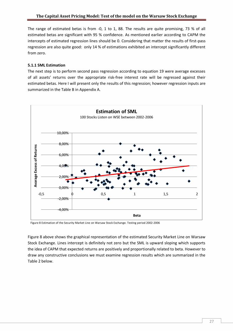
5.1.1 SML Estimation
The next step is to perform second pass regression according to equation 19 were average excesses
of all assets’ returns over the appropriate risk-free interest rate will be regressed against their
estimated betas. Here I will present only the results of this regression; however regression inputs are
summarized in the Table B in Appendix A.
Figure 8 Estimation of the Security Market Line on Warsaw Stock Exchange. Testing period 2002-2006
Figure 8 above shows the graphical representation of the estimated Security Market Line on Warsaw
Stock Exchange. Lines intercept is definitely not zero but the SML is upward sloping which supports
the idea of CAPM that expected returns are positively and proportionally related to beta. However to
draw any constructive conclusions we must examine regression results which are summarized in the
Table 2 below.
-4,00%
-2,00%
0,00%
2,00%
4,00%
6,00%
8,00%
10,00%
-0,5 0 0,5 1 1,5 2
Ava
rage
Exc
ess
of
Ret
urn
s
Beta
Estimation of SML100 Stocks Listen on WSE between 2002-2006
The Capital Asset Pricing Model: Test of the model on the Warsaw Stock Exchange
28
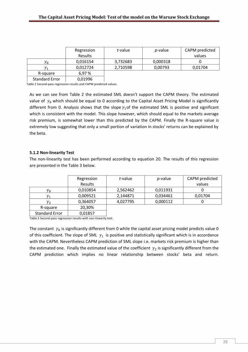
Table 2 Second-pass regression results and CAPM predicted values.
As we can see from Table 2 the estimated SML doesn’t support the CAPM theory. The estimated
value of which should be equal to 0 according to the Capital Asset Pricing Model is significantly
different from 0. Analysis shows that the slope of the estimated SML is positive and significant
which is consistent with the model. This slope however, which should equal to the markets average
risk premium, is somewhat lower than this predicted by the CAPM. Finally the R-square value is
extremely low suggesting that only a small portion of variation in stocks’ returns can be explained by
the beta.
5.1.2 Non-linearity Test
The non-linearity test has been performed according to equation 20. The results of this regression
are presented in the Table 3 below.
Regression Results
t-value p-value CAPM predicted values
0,010854 2,562462 0,011931 0
0,009521 2,144871 0,034461 0,01704
0,364057 4,027795 0,000112 0
R-square 20,30%
Standard Error 0,01857 Table 3 Second-pass regression results with non-linearity test.
The constant is significantly different from 0 while the capital asset pricing model predicts value 0
of this coefficient. The slope of SML is positive and statistically significant which is in accordance
with the CAPM. Nevertheless CAPM prediction of SML slope i.e. markets risk premium is higher than
the estimated one. Finally the estimated value of the coefficient is significantly different from the
CAPM prediction which implies no linear relationship between stocks’ beta and return.
Regression Results
t-value p-value CAPM predicted values
0,016154 3,732683 0,000318 0
0,012724 2,710598 0,00793 0,01704
R-square 6,97 %
Standard Error 0,01996

The Capital Asset Pricing Model: Test of the model on the Warsaw Stock Exchange
29
5.1.3Non-systematic risk Test.
To perform test for non-systematic risk I will utilize equation 21. The results of the regression are
presented in the Table 4:
Regression Results
t-value p-value CAPM predicted values
0,010694 1,766897 0,080424 0
0,010029 0,699723 0,485792 0,01704
0,364115 4,007061 0,000121 0
– 0,0003 – 0,03731 0,970318 0
R-square 20,30%
Standard Error 0,018666 Table 4 Second-pass regression results with non-linearity and non-systematic risk test.
Regressions intercept is insignificantly different from 0 which is consistent with the CAPM
prediction. The estimated average markets’ risk-premium is positive but insignificant and lower
than the premium predicted by the model. Significant estimation of implies no linear relationship
between beta and return. Finally the estimated value of coefficient is insignificantly different
from 0 which is with accordance with the CAPM. It implies that all the risk is captured by beta and
non-systematic risk has no influence on stocks’ returns.
5.2 Black, Jensen and Scholes Test I will start the test with summarizing all the testing sub-periods for convenience:
Sub-period 1 Sub-period 2 Sub-period 2
Stocks’ beta estimation 2002-2003 2003-2004 2004-2005
Portfolio creation date 31-12-2003 31-12-2004 31-12-2005
Portfolio returns computation
2004 2005 2006
Table 5 Testing sub-periods in the BJS test
The stocks’ betas have been calculated according to equation 18 in each of the 3 sub-periods. The
complete results of these regressions are presented in Tables A-C in Appendix B. In years 2002-2003
40 % of estimated betas are significant while 91 % of estimated intercepts are insignificantly different
from 0. Estimates in the next sub-period are somewhat better: 61 % significant betas and 96 %
intercepts insignificantly different from 0. In the last sub-period the corresponding percentages are
30 % for betas and 89 % for intercepts.
After estimating the betas 10 portfolios have been constructed based on these betas. The content of
each portfolio in corresponding sub-period is presented in the Table 6.

The Capital Asset Pricing Model: Test of the model on the Warsaw Stock Exchange
30
PORTFOLIO 1
2003 Beta t-value 2004 Beta t-value 2005 Beta3 t-value
06MAGNA -0,36 -2,36 SWIECIE -0,56 -1,60 TUEUROPA -1,47 -1,36
SWIECIE -0,21 -0,87 MIESZKO -0,22 -0,35 05VICT -1,28 -1,35
INDYKPOL -0,11 -0,44 13FORTUNA -0,15 -0,35 MENNICA -0,95 -1,26
ABG -0,09 -0,25 DZPOLSKA -0,08 -0,19 WISTIL -0,73 -1,24
MOSTALWAR -0,01 -0,02 06MAGNA -0,08 -0,62 Jupiter -0,71 -1,12
13FORTUNA 0,02 0,10 01NFI -0,07 -0,16 PPWK -0,47 -0,54
08OCTAVA 0,03 0,05 05VICT -0,07 -0,16 MUZA -0,33 -0,50
MIESZKO 0,04 0,22 08OCTAVA -0,01 -0,01 KROSNO -0,28 -0,60
05VICT 0,05 0,24 TUEUROPA 0,09 0,11 01NFI -0,27 -0,25
01NFI 0,10 0,70 MENNICA 0,10 0,18 06MAGNA -0,23 -0,81
PORTFOLIO 2
2003 Beta t-value 2004 Beta2 t-value 2005 Beta t-value
04PRO 0,11 0,61 MOSTALWAR 0,12 0,24 Kruszwica -0,18 -0,40
FORTISPL 0,12 0,33 ABG 0,16 0,26 DEBICA -0,17 -0,60
UNIMIL 0,12 0,36 Jupiter 0,18 0,50 IRENA -0,15 -0,50
APATOR 0,14 0,38 UNIMIL 0,21 0,49 08OCTAVA -0,04 -0,09
02NFI 0,15 0,56 04PRO 0,26 0,69 Sanok -0,03 -0,08
Jupiter 0,17 0,85 APATOR 0,29 0,66 WAWEL -0,03 -0,06
TUEUROPA 0,20 0,76 INDYKPOL 0,29 0,39 RELPOL -0,01 -0,03
MUZA 0,24 0,51 BOS 0,33 1,93 Zywiec 0,01 0,09
ENERGOPN 0,27 0,33 ENERGOPN 0,34 0,35 SWIECIE 0,02 0,07
INGBSK 0,33 1,68 MUZA 0,37 0,65 LPP 0,06 0,16
PORTFOLIO 3
2003 Beta t-value 2004 Beta t-value 2005 Beta t-value
MENNICA 0,39 1,66 FORTISPL 0,41 1,15 DZPOLSKA 0,06 0,09
KredytBank 0,40 1,87 INGBSK 0,42 1,58 MIESZKO 0,08 0,09
BOS 0,41 2,01 COMPLAND 0,48 1,59 ELDORADO 0,09 0,29
IRENA 0,41 1,86 02NFI 0,48 1,32 02NFI 0,13 0,26
MostalZab 0,44 0,71 Millennium 0,57 2,01 MOSTALPLC 0,14 0,19
AMICA 0,49 1,51 WAWEL 0,57 2,09 TALEX 0,17 0,27
NORDEABP 0,49 1,23 Zywiec 0,57 3,05 POLIMEXMS 0,17 0,21
Optimus 0,51 1,56 FARMACOL 0,58 1,29 KABLE 0,18 0,15
WAWEL 0,55 2,76 DEBICA 0,60 2,35 BUDIMEX 0,24 0,53
STRZELEC 0,57 1,67 MOSTALPLC 0,63 1,50 POLLENAE 0,25 0,49
PORTFOLIO 4
2003 Beta t-value 2004 Beta t-value 2005 Beta t-value
ELDORADO 0,58 2,73 IRENA 0,67 2,49 GRAJEWO 0,26 0,71
Handlowy 0,58 3,75 MostalZab 0,68 0,92 STALPROD 0,30 0,44
POLNORD 0,59 1,89 TALEX 0,69 1,54 04PRO 0,31 0,56
GRAJEWO 0,60 1,66 CSS 0,70 4,08 PGF 0,38 1,37
PROCHEM 0,61 2,73 Optimus 0,71 2,14 KOGENERA 0,38 0,56
NOVITA 0,61 1,21 AMICA 0,73 1,54 NOVITA 0,42 0,55
CSS 0,63 2,00 Groclin 0,76 2,91 IMPEXMET 0,43 0,76
MOSTALPLC 0,63 4,34 VISTULA 0,76 0,94 Groclin 0,47 1,05
Zywiec 0,64 3,70 KredytBank 0,77 2,91 Handlowy 0,47 1,68
Kopex 0,69 1,10 PKNORLEN 0,78 6,27 NORDEABP 0,49 0,91

The Capital Asset Pricing Model: Test of the model on the Warsaw Stock Exchange
31
PORTFOLIO 5
2003 Beta t-value 2004 Beta t-value 2005 Beta t-value
PGF 0,70 3,87 ELEKTRIM 0,81 1,26 PROCHEM 0,49 0,65
COMPLAND 0,70 3,00 WANDALEX 0,82 1,29 COMARCH 0,50 1,66
DZPOLSKA 0,71 1,80 Handlowy 0,86 4,09 AGORA 0,52 1,48
ELBUDOWA 0,72 3,11 PGF 0,87 4,27 KETY 0,55 1,74
DEBICA 0,73 4,44 LENTEX 0,88 2,57 ECHO 0,55 1,50
INSTALKRK 0,73 1,40 MostalExp 0,88 2,05 TIM 0,55 0,64
KROSNO 0,74 2,67 TPSA 0,90 4,76 ORBIS 0,56 1,77
EFEKT 0,75 1,76 PROCHEM 0,91 1,70 Jutrzenka 0,58 0,92
FORTE 0,78 2,82 KROSNO 0,92 2,44 BOS 0,58 1,74
FARMACOL 0,79 2,31 ELBUDOWA 0,92 2,18 WANDALEX 0,59 0,86
PORTFOLIO 6
2003 Beta t-value 2004 Beta2 t-value 2005 Beta t-value
ECHO 0,83 3,46 BZWBK 0,94 7,44 LENTEX 0,62 1,27
KETY 0,84 4,43 KOGENERA 0,94 2,31 ELEKTRIM 0,65 0,69
STALPROD 0,84 2,35 Kopex 0,95 1,29 VISTULA 0,65 0,88
PKNORLEN 0,86 5,62 MNI 0,96 1,36 AMICA 0,65 1,23
Millennium 0,87 3,68 LPP 0,96 2,49 FARMACOL 0,66 2,34
VISTULA 0,90 1,44 PEKAO 1,00 7,61 BORYSZEW 0,71 0,94
PEKAO 0,91 7,29 POLNORD 1,00 2,13 COMPLAND 0,72 2,01
WANDALEX 0,92 2,12 NORDEABP 1,01 2,11 INGBSK 0,74 2,93
BZWBK 0,92 6,41 INSTALKRK 1,01 1,80 CERSANIT 0,77 3,45
CERSANIT 0,93 1,77 GRAJEWO 1,02 2,32 Netia 0,79 2,60
PORTFOLIO 7
2003 Beta t-value 2004 Beta2 t-value 2005 Beta t-value
Groclin 0,93 3,49 CERSANIT 1,03 6,72 STALEXP 0,79 1,21
LPP 0,94 2,69 ELDORADO 1,03 4,97 BEDZIN 0,80 1,72
BEDZIN 0,94 1,66 Jutrzenka 1,03 3,73 13FORTUNA 0,83 0,92
AGORA 0,95 4,50 KETY 1,06 4,14 EFEKT 0,84 1,43
RELPOL 0,96 3,94 AGORA 1,09 4,41 Optimus 0,86 1,78
KOGENERA 0,97 2,68 STRZELEC 1,09 2,20 POLNORD 0,86 1,15
LENTEX 0,99 3,60 Netia 1,10 4,73 FORTISPL 0,87 2,18
TPSA 1,04 6,07 COMARCH 1,11 4,60 CSS 0,89 3,16
Sanok 1,07 3,06 BUDIMEX 1,14 4,38 BRE 0,96 3,77
Jutrzenka 1,08 5,50 EFEKT 1,15 2,90 GETIN 0,97 1,45
PORTFOLIO 8
2003 Beta t-value 2004 Beta t-value 2005 Beta t-value
TALEX 1,10 3,13 TIM 1,17 1,88 PROSPER 1,01 2,80
WILBO 1,13 4,97 BANKBPH 1,20 6,47 FORTE 1,01 3,06
BUDIMEX 1,14 6,56 PPWK 1,20 2,32 MNI 1,01 1,90
ELEKTRIM 1,19 2,52 Prokom 1,28 4,92 INDYKPOL 1,07 0,96
Ferrum 1,20 1,60 FORTE 1,28 4,18 ABG 1,10 1,73
COMARCH 1,24 5,79 WILBO 1,29 3,75 UNIMIL 1,18 2,55
PPWK 1,26 2,36 BRE 1,31 4,62 Ferrum 1,20 1,31
BANKBPH 1,29 7,23 RELPOL 1,31 5,19 KredytBank 1,20 4,34
PROVIMROL 1,32 4,84 KGHM 1,35 4,93 WILBO 1,23 2,44
KGHM 1,33 6,36 NOVITA 1,40 2,21 BANKBPH 1,24 6,25
The Capital Asset Pricing Model: Test of the model on the Warsaw Stock Exchange
32
PORTFOLIO 9
2003 Beta t-value 2004 Beta t-value 2005 Beta t-value
Prokom 1,34 6,11 GETIN 1,46 2,29 ENERGOPN 1,26 2,04
BRE 1,35 4,97 STALEXP 1,47 2,73 PKNORLEN 1,29 5,72
TIM 1,37 3,65 STALPROD 1,49 3,03 Kopex 1,30 3,16
MostalExp 1,40 2,81 BEDZIN 1,49 2,53 MOSTALWAR 1,36 1,75
MCI 1,44 3,51 ECHO 1,49 7,40 PEKAO 1,36 7,21
PROSPER 1,53 4,03 ORBIS 1,58 5,85 APATOR 1,37 3,09
BORYSZEW 1,54 2,46 Sanok 1,66 3,74 MostalZab 1,42 1,40
POLLENAE 1,61 4,08 PROSPER 1,68 4,08 MostalExp 1,46 3,04
STALEXP 1,62 4,21 IMPEXMET 1,68 3,33 INSTALKRK 1,46 2,78
ORBIS 1,64 6,90 MCI 1,69 1,78 ELBUDOWA 1,48 2,62
PORTFOLIO 10
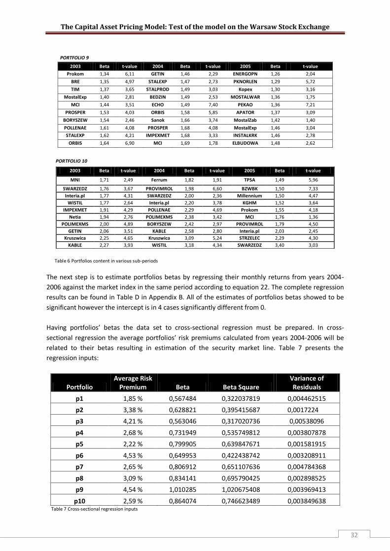
Table 6 Portfolios content in various sub-periods
The next step is to estimate portfolios betas by regressing their monthly returns from years 2004-
2006 against the market index in the same period according to equation 22. The complete regression
results can be found in Table D in Appendix B. All of the estimates of portfolios betas showed to be
significant however the intercept is in 4 cases significantly different from 0.
Having portfolios’ betas the data set to cross-sectional regression must be prepared. In cross-
sectional regression the average portfolios’ risk premiums calculated from years 2004-2006 will be
related to their betas resulting in estimation of the security market line. Table 7 presents the
regression inputs:
Portfolio Average Risk
Premium Beta Beta Square Variance of Residuals
p1 1,85 % 0,567484 0,322037819 0,004462515
p2 3,38 % 0,628821 0,395415687 0,0017224
p3 4,21 % 0,563046 0,317020736 0,00538096
p4 2,68 % 0,731949 0,535749812 0,003807878
p5 2,22 % 0,799905 0,639847671 0,001581915
p6 4,53 % 0,649953 0,422438742 0,003208911
p7 2,65 % 0,806912 0,651107636 0,004784368
p8 3,09 % 0,834141 0,695790425 0,002898525
p9 4,54 % 1,010285 1,020675408 0,003969413
p10 2,59 % 0,864074 0,746623489 0,003849638 Table 7 Cross-sectional regression inputs
2003 Beta t-value 2004 Beta t-value 2005 Beta t-value
MNI 1,71 2,49 Ferrum 1,82 1,91 TPSA 1,49 5,96
SWARZEDZ 1,76 3,67 PROVIMROL 1,98 6,60 BZWBK 1,50 7,33
Interia.pl 1,77 4,31 SWARZEDZ 2,00 2,36 Millennium 1,50 4,47
WISTIL 1,77 2,64 Interia.pl 2,20 3,78 KGHM 1,52 3,64
IMPEXMET 1,91 4,29 POLLENAE 2,29 4,69 Prokom 1,55 4,18
Netia 1,94 2,76 POLIMEXMS 2,38 3,42 MCI 1,76 1,36
POLIMEXMS 2,00 4,89 BORYSZEW 2,42 2,97 PROVIMROL 1,79 4,50
GETIN 2,06 3,51 KABLE 2,58 2,80 Interia.pl 2,03 2,45
Kruszwica 2,25 4,65 Kruszwica 3,09 5,24 STRZELEC 2,29 4,30
KABLE 2,27 3,93 WISTIL 3,18 4,34 SWARZEDZ 3,40 3,03
The Capital Asset Pricing Model: Test of the model on the Warsaw Stock Exchange
33
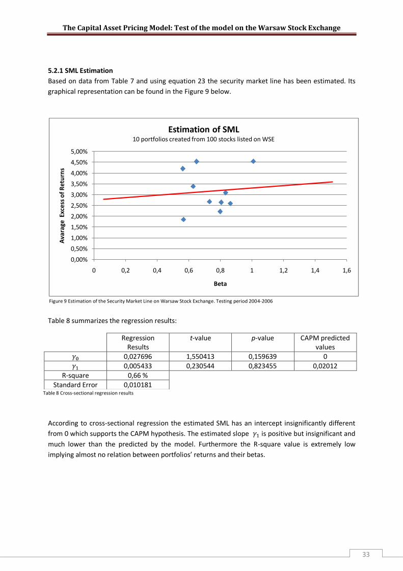
5.2.1 SML Estimation
Based on data from Table 7 and using equation 23 the security market line has been estimated. Its
graphical representation can be found in the Figure 9 below.
Figure 9 Estimation of the Security Market Line on Warsaw Stock Exchange. Testing period 2004-2006
Table 8 summarizes the regression results:
Table 8 Cross-sectional regression results
According to cross-sectional regression the estimated SML has an intercept insignificantly different
from 0 which supports the CAPM hypothesis. The estimated slope is positive but insignificant and
much lower than the predicted by the model. Furthermore the R-square value is extremely low
implying almost no relation between portfolios’ returns and their betas.
0,00%
0,50%
1,00%
1,50%
2,00%
2,50%
3,00%
3,50%
4,00%
4,50%
5,00%
0 0,2 0,4 0,6 0,8 1 1,2 1,4 1,6
Ava
rage
Exc
ess
of
Re
turn
s
Beta
Estimation of SML10 portfolios created from 100 stocks listed on WSE
Regression Results
t-value p-value CAPM predicted values
0,027696 1,550413 0,159639 0
0,005433 0,230544 0,823455 0,02012
R-square 0,66 %
Standard Error 0,010181
The Capital Asset Pricing Model: Test of the model on the Warsaw Stock Exchange
34
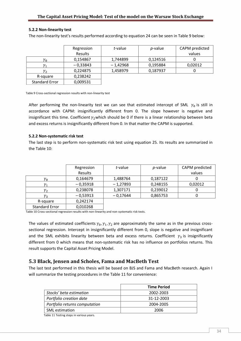
5.2.2 Non-linearity test
The non-linearity test’s results performed according to equation 24 can be seen in Table 9 below:
Table 9 Cross-sectional regression results with non-linearity test
After performing the non-linearity test we can see that estimated intercept of SML is still in
accordance with CAPM: insignificantly different from 0. The slope however is negative and
insignificant this time. Coefficient which should be 0 if there is a linear relationship between beta
and excess returns is insignificantly different from 0. In that matter the CAPM is supported.
5.2.2 Non-systematic risk test
The last step is to perform non-systematic risk test using equation 25. Its results are summarized in
the Table 10:
Regression Results
t-value p-value CAPM predicted values
0,164679 1,488764 0,187122 0
– 0,35918 – 1,27893 0,248155 0,02012
0,238078 1,307171 0,239012 0
– 0,53913 – 0,17644 0,865753 0
R-square 0,242174
Standard Error 0,010268 Table 10 Cross-sectional regression results with non-linearity and non-systematic risk tests.
The values of estimated coefficients are approximately the same as in the previous cross-
sectional regression. Intercept in insignificantly different from 0, slope is negative and insignificant
and the SML exhibits linearity between beta and excess returns. Coefficient is insignificantly
different from 0 which means that non-systematic risk has no influence on portfolios returns. This
result supports the Capital Asset Pricing Model.
5.3 Black, Jensen and Scholes, Fama and MacBeth Test The last test performed in this thesis will be based on BJS and Fama and MacBeth research. Again I
will summarize the testing procedures in the Table 11 for convenience:
Time Period
Stocks’ beta estimation 2002-2003
Portfolio creation date 31-12-2003
Portfolio returns computation 2004-2005
SML estimation 2006 Table 11 Testing steps in various years.
Regression Results
t-value p-value CAPM predicted values
0,154867 1,744899 0,124516 0
– 0,33843 – 1,42968 0,195884 0,02012
0,224875 1,458979 0,187937 0
R-square 0,238242
Standard Error 0,009531
The Capital Asset Pricing Model: Test of the model on the Warsaw Stock Exchange
35
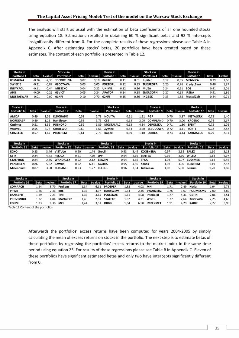
The analysis will start as usual with the estimation of beta coefficients of all one hounded stocks
using equation 18. Estimations resulted in obtaining 60 % significant betas and 92 % intercepts
insignificantly different from 0. For the complete results of these regressions please see Table A in
Appendix C. After estimating stocks’ betas, 20 portfolios have been created based on these
estimates. The content of each portfolio is presented in Table 12.
Stocks in
Portfolio 1 Beta t-value Stocks in
Portfolio 2 Beta t-value Stocks in
Portfolio 3 Beta t-value Stocks in
Portfolio 4 Beta t-value Stocks in
Portfolio 5 Beta t-value
06MAGNA -0,36 -2,36 13FORTUNA 0,02 0,10 04PRO 0,11 0,61 Jupiter 0,17 0,85 MENNICA 0,39 1,66
SWIECIE -0,21 -0,87 08OCTAVA 0,03 0,05 FORTISPL 0,12 0,33 TUEUROPA 0,20 0,76 KredytBank 0,40 1,87
INDYKPOL -0,11 -0,44 MIESZKO 0,04 0,22 UNIMIL 0,12 0,36 MUZA 0,24 0,51 BOS 0,41 2,01
ABG -0,09 -0,25 05VICT 0,05 0,24 APATOR 0,14 0,38 ENERGOPN 0,27 0,33 IRENA 0,41 1,86
MOSTALWAR -0,01 -0,02 01NFI 0,10 0,70 02NFI 0,15 0,56 INGBSK 0,33 1,68 MostalZab 0,44 0,71
Stocks in
Portfolio 6 Beta t-value Stocks in
Portfolio 7 Beta t-value Stocks in
Portfolio 8 Beta t-value Stocks in
Portfolio 9 Beta t-value Stocks in
Portfolio 10 Beta t-value
AMICA 0,49 1,51 ELDORADO 0,58 2,73 NOVITA 0,61 1,21 PGF 0,70 3,87 INSTALKRK 0,73 1,40
NORDEABP 0,49 1,23 Handlowy 0,58 3,75 CSS 0,63 2,00 COMPLAND 0,70 3,00 KROSNO 0,74 2,67
Optimus 0,51 1,56 POLNORD 0,59 1,89 MOSTALPLC 0,63 4,34 DZPOLSKA 0,71 1,80 EFEKT 0,75 1,76
WAWEL 0,55 2,76 GRAJEWO 0,60 1,66 Zywiec 0,64 3,70 ELBUDOWA 0,72 3,11 FORTE 0,78 2,82
STRZELEC 0,57 1,67 PROCHEM 0,61 2,73 Kopex 0,69 1,10 DEBICA 0,73 4,44 FARMACOL 0,79 2,31
Stocks in
Portfolio 16 Beta t-value Stocks in
Portfolio 17 Beta t-value Stocks in
Portfolio 18 Beta t-value Stocks in
Portfolio 19 Beta t-value Stocks in
Portfolio 20 Beta t-value
COMARCH 1,24 5,79 Prokom 1,34 6,11 PROSPER 1,53 4,03 MNI 1,71 2,49 Netia 1,94 2,76
PPWK 1,26 2,36 BRE 1,35 4,97 BORYSZEW 1,54 2,46 SWARZEDZ 1,76 3,67 POLIMEXMS 2,00 4,89
BANKBPH 1,29 7,23 TIM 1,37 3,65 POLLENAE 1,61 4,08 Interia.pl 1,77 4,31 GETIN 2,06 3,51
PROVIMROL 1,32 4,84 MostalExp 1,40 2,81 STALEXP 1,62 4,21 WISTIL 1,77 2,64 Kruszwica 2,25 4,65
KGHM 1,33 6,36 MCI 1,44 3,51 ORBIS 1,64 6,90 IMPEXMET 1,91 4,29 KABLE 2,27 3,93
Table 12 Content of the portfolios
Afterwards the portfolios’ excess returns have been computed for years 2004-2005 by simply
calculating the mean of excess returns on stocks in the portfolio. The next step is to estimate betas of
these portfolios by regressing the portfolios’ excess returns to the market index in the same time
period using equation 23. For results of these regressions please see Table B in Appendix C. Eleven of
these portfolios have significant estimated betas and only two have intercepts significantly different
from 0.
Stocks in Portfolio 11 Beta t-value
Stocks in Portfolio 12 Beta t-value
Stocks in Portfolio 13 Beta t-value
Stocks in Portfolio 14 Beta t-value
Stocks in Portfolio 15 Beta t-value
ECHO 0,83 3,46 VISTULA 0,90 1,44 Groclin 0,93 3,49 KOGENERA 0,97 2,68 TALEX 1,10 3,13
KETY 0,84 4,43 PEKAO 0,91 7,29 LPP 0,94 2,69 LENTEX 0,99 3,60 WILBO 1,13 4,97
STALPROD 0,84 2,35 WANDALEX 0,92 2,12 BEDZIN 0,94 1,66 TPSA 1,04 6,07 BUDIMEX 1,14 6,56
PKNORLEN 0,86 5,62 BZWBK 0,92 6,41 AGORA 0,95 4,50 Sanok 1,07 3,06 ELEKTRIM 1,19 2,52
Millennium 0,87 3,68 CERSANIT 0,93 1,77 RELPOL 0,96 3,94 Jutrzenka 1,08 5,50 Ferrum 1,20 1,60

The Capital Asset Pricing Model: Test of the model on the Warsaw Stock Exchange
36
Now everything is ready to perform the cross-section regression and estimate the security market
line in the year 2006. The regression inputs are presented in Table 13:
Table 13 Inputs to cross-section regression
5.3.1 SML Estimation
Using the data from Table 13 and equation 23 the security market line has been estimated. It is
presented in the Figure 10 below:
Figure 10 Estimation of the Security Market Line on Warsaw Stock Exchange. Testing year 2006
0,00%
2,00%
4,00%
6,00%
8,00%
10,00%
12,00%
-0,4 -0,2 0 0,2 0,4 0,6 0,8 1 1,2 1,4
Ava
rage
Exc
ess
of
Re
turn
s
Beta
Estimation of SML20 portfolios containing stocks listed on the WSE
Portfolio Average Excess returns in 2006
Beta Beta Square Variance of residuals
p1 6,18% 0,662537 0,438956 0,010414
p2 0,79% -0,13477 0,018162 0,014431
p3 6,95% 0,770993 0,59443 0,013204
p4 6,16% -0,10452 0,010924 0,028409
p5 3,98% 0,420572 0,176881 0,016108
p6 2,33% 0,852132 0,726129 0,014699
p7 10,54% 0,431808 0,186458 0,009582
p8 8,75% 0,552562 0,305325 0,022143
p9 5,65% 0,492158 0,242219 0,008926
p10 4,13% 0,738256 0,545021 0,020009
p11 6,49% 0,838578 0,703212 0,008299
p12 6,40% 0,973739 0,948168 0,024395
p13 0,75% 0,366502 0,134324 0,016944
p14 5,19% 0,607397 0,368931 0,010931
p15 9,82% 0,697025 0,485845 0,027274
p16 6,00% 0,915004 0,837232 0,012939
p17 6,18% 1,253952 1,572396 0,018736
p18 5,51% 0,664625 0,441726 0,024692
p19 6,25% 1,226472 1,504234 0,041869
p20 8,64% 0,386471 0,149359 0,043445
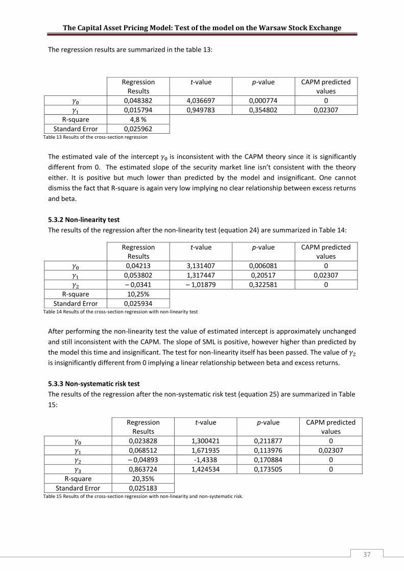
The Capital Asset Pricing Model: Test of the model on the Warsaw Stock Exchange
37
The regression results are summarized in the table 13:
Table 13 Results of the cross-section regression
The estimated vale of the intercept is inconsistent with the CAPM theory since it is significantly
different from 0. The estimated slope of the security market line isn’t consistent with the theory
either. It is positive but much lower than predicted by the model and insignificant. One cannot
dismiss the fact that R-square is again very low implying no clear relationship between excess returns
and beta.
5.3.2 Non-linearity test
The results of the regression after the non-linearity test (equation 24) are summarized in Table 14:
Table 14 Results of the cross-section regression with non-linearity test
After performing the non-linearity test the value of estimated intercept is approximately unchanged
and still inconsistent with the CAPM. The slope of SML is positive, however higher than predicted by
the model this time and insignificant. The test for non-linearity itself has been passed. The value of
is insignificantly different from 0 implying a linear relationship between beta and excess returns.
5.3.3 Non-systematic risk test
The results of the regression after the non-systematic risk test (equation 25) are summarized in Table
15:
Table 15 Results of the cross-section regression with non-linearity and non-systematic risk.
Regression Results
t-value p-value CAPM predicted values
0,048382 4,036697 0,000774 0
0,015794 0,949783 0,354802 0,02307
R-square 4,8 %
Standard Error 0,025962
Regression Results
t-value p-value CAPM predicted values
0,04213 3,131407 0,006081 0
0,053802 1,317447 0,20517 0,02307
– 0,0341 – 1,01879 0,322581 0
R-square 10,25%
Standard Error 0,025934
Regression Results
t-value p-value CAPM predicted values
0,023828 1,300421 0,211877 0
0,068512 1,671935 0,113976 0,02307
– 0,04893 -1,4338 0,170884 0
0,863724 1,424534 0,173505 0
R-square 20,35%
Standard Error 0,025183

The Capital Asset Pricing Model: Test of the model on the Warsaw Stock Exchange
38
The results suggest that the intercept of the estimated SML, which is insignificantly different from 0,
is in accordance with CAPM. The slope however is even higher than in previous test and still
insignificant. Non-linearity test has been passed again. It would also seem that non-systematic risk
has no influence on the portfolios’ risk premiums since is insignificantly different from 0, thus
consistent with the theory of CAMP.
Daddy
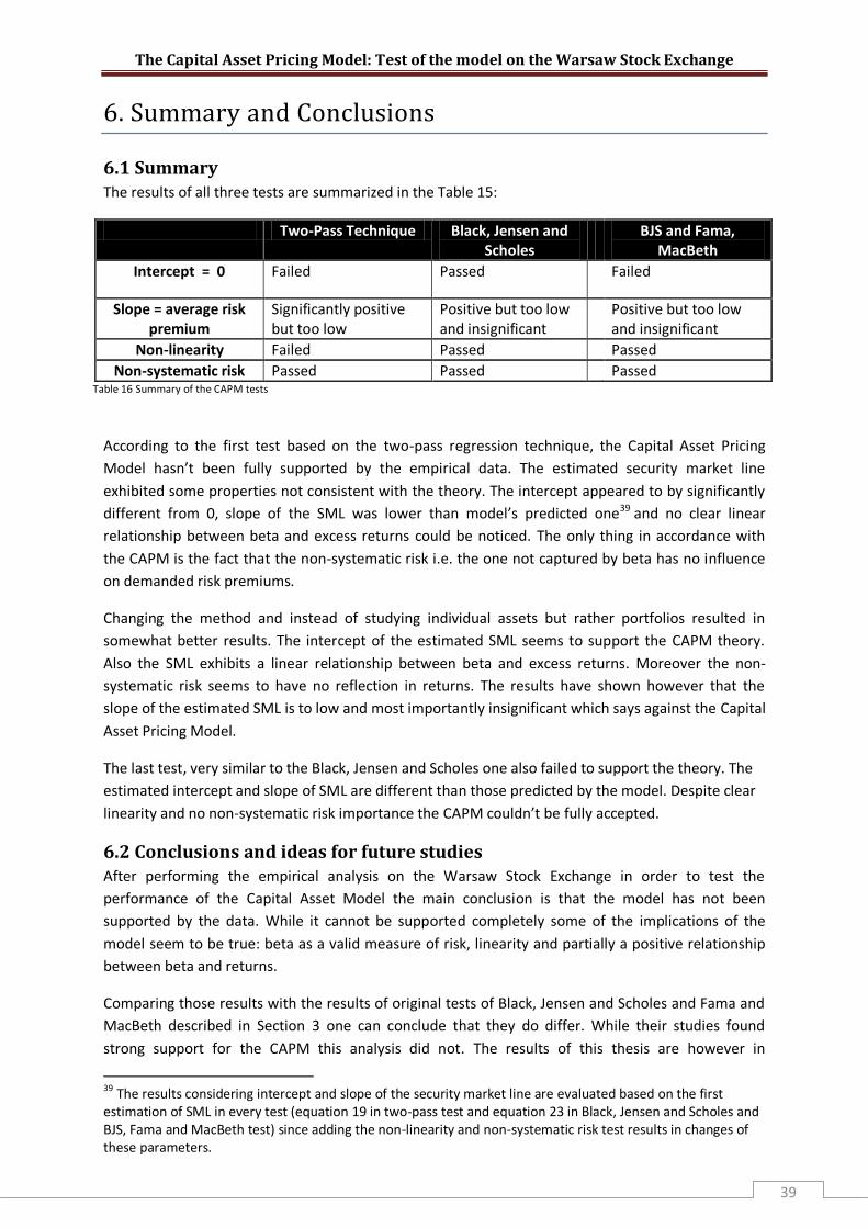
The Capital Asset Pricing Model: Test of the model on the Warsaw Stock Exchange
39
6. Summary and Conclusions
6.1 Summary The results of all three tests are summarized in the Table 15:
Two-Pass Technique Black, Jensen and Scholes
BJS and Fama, MacBeth
Intercept = 0 Failed Passed Failed
Slope = average risk premium
Significantly positive but too low
Positive but too low and insignificant
Positive but too low and insignificant
Non-linearity Failed Passed Passed
Non-systematic risk Passed Passed Passed Table 16 Summary of the CAPM tests
According to the first test based on the two-pass regression technique, the Capital Asset Pricing
Model hasn’t been fully supported by the empirical data. The estimated security market line
exhibited some properties not consistent with the theory. The intercept appeared to by significantly
different from 0, slope of the SML was lower than model’s predicted one39 and no clear linear
relationship between beta and excess returns could be noticed. The only thing in accordance with
the CAPM is the fact that the non-systematic risk i.e. the one not captured by beta has no influence
on demanded risk premiums.
Changing the method and instead of studying individual assets but rather portfolios resulted in
somewhat better results. The intercept of the estimated SML seems to support the CAPM theory.
Also the SML exhibits a linear relationship between beta and excess returns. Moreover the non-
systematic risk seems to have no reflection in returns. The results have shown however that the
slope of the estimated SML is to low and most importantly insignificant which says against the Capital
Asset Pricing Model.
The last test, very similar to the Black, Jensen and Scholes one also failed to support the theory. The
estimated intercept and slope of SML are different than those predicted by the model. Despite clear
linearity and no non-systematic risk importance the CAPM couldn’t be fully accepted.
6.2 Conclusions and ideas for future studies After performing the empirical analysis on the Warsaw Stock Exchange in order to test the
performance of the Capital Asset Model the main conclusion is that the model has not been
supported by the data. While it cannot be supported completely some of the implications of the
model seem to be true: beta as a valid measure of risk, linearity and partially a positive relationship
between beta and returns.
Comparing those results with the results of original tests of Black, Jensen and Scholes and Fama and
MacBeth described in Section 3 one can conclude that they do differ. While their studies found
strong support for the CAPM this analysis did not. The results of this thesis are however in
39
The results considering intercept and slope of the security market line are evaluated based on the first estimation of SML in every test (equation 19 in two-pass test and equation 23 in Black, Jensen and Scholes and BJS, Fama and MacBeth test) since adding the non-linearity and non-systematic risk test results in changes of these parameters.
The Capital Asset Pricing Model: Test of the model on the Warsaw Stock Exchange
40
accordance with studies performed after 1965 like Fench 1980 or Fama and French 1992 which
rejected the model. These studies however allowed more variables than just beta to influence stocks’
expected return so one should be careful in comparing the results of these studies.
One must bear in mind that the version of the CAPM tested in this model is the most basic one and it
is based on quite strong assumptions. Remember that we assumed for instance no market
imperfections (taxes, transaction costs) or same access to information for all investors. Perhaps by
modifying or reliving some of the assumptions the results would be better. There are also some
versions of the CAPM putting the restrictions on the risk-free asset such as the Black versions which
assumes lack of such an asset on the market or the CAPM when lending at risk-free rate is possible
but not borrowing. Maybe these versions could find a support of empirical data. At this point it is also
important to remember that the index WIG was used as a proxy of the market and the market
portfolio. One must bear in mind that this index contains only common stocks but theory assumes
that market portfolio contains all tradeable assets including not only stocks, bonds, options, futures
but even real estate and human capital. In that case the proxy of the market used in this paper is
hardly a realistic one.
A good idea for future study of assets traded on the Warsaw Stock Exchange could be to test a theory
developed after the CAPM namely the Arbitrage Pricing Theory, which allows more factors than just
beta to influence securities’ rate of returns.
The Capital Asset Pricing Model: Test of the model on the Warsaw Stock Exchange
41
7. References
Bodie Ziv , Merton Robert C. [2000] “Finance” International Edition Prentice
Hall, New Jersey
Brealey, Myers, Allen [2006] “Corporate Finance” 8th Edition McGraw-Hill, New
York
Campbell John Y., Lo Andrwe W., MacKinlay Craig A. [1997] “The Econometrics
of Financial Markets” 2nd Edition Princeton University Press, New Jersey
Copeland Thomas E., Weston Fred J. Shastri Kuldeep [2005] “Financial Theory
and Corporate Policy” 4th Edition Pearson Education
Haugen Robert A. [2001] “Modern Investment Theory” 5th Edition Prentice-Hall,
New Jersey
Grigoris Michailidis, Stavros Tsopoglou, Demetrios Papanastasiou, Eleni Mariola
[2006] “Testing the Capital Asset Pricing Model (CAPM): The Case of the
Emerging Greek Securities Market” International Research Journal of Finance
and Economics Issue 4,
Markowitz Harry [1952] “Portfolio Selection” Journal of Finance Vol. VII, No.1
Sørensen Peter Birch, Whitta-Jacobsen Hans Jørgen [2005] ”Introducing
Advanced Macroeconomics: Growth & Business Cycles” McGraw-Hill Berkshire
“Fact Book 2006” Official publication of the Warsaw Stock Exchange
Warsaw Stock Exchange Official Quotations
http://www.gpw.com.pl/gpw.asp?cel=informacje_gieldowe&k=15&i=/statystyk
i/miesieczne&sky=1
Official Statistics of the Polish Central Bank www.nbp.pl
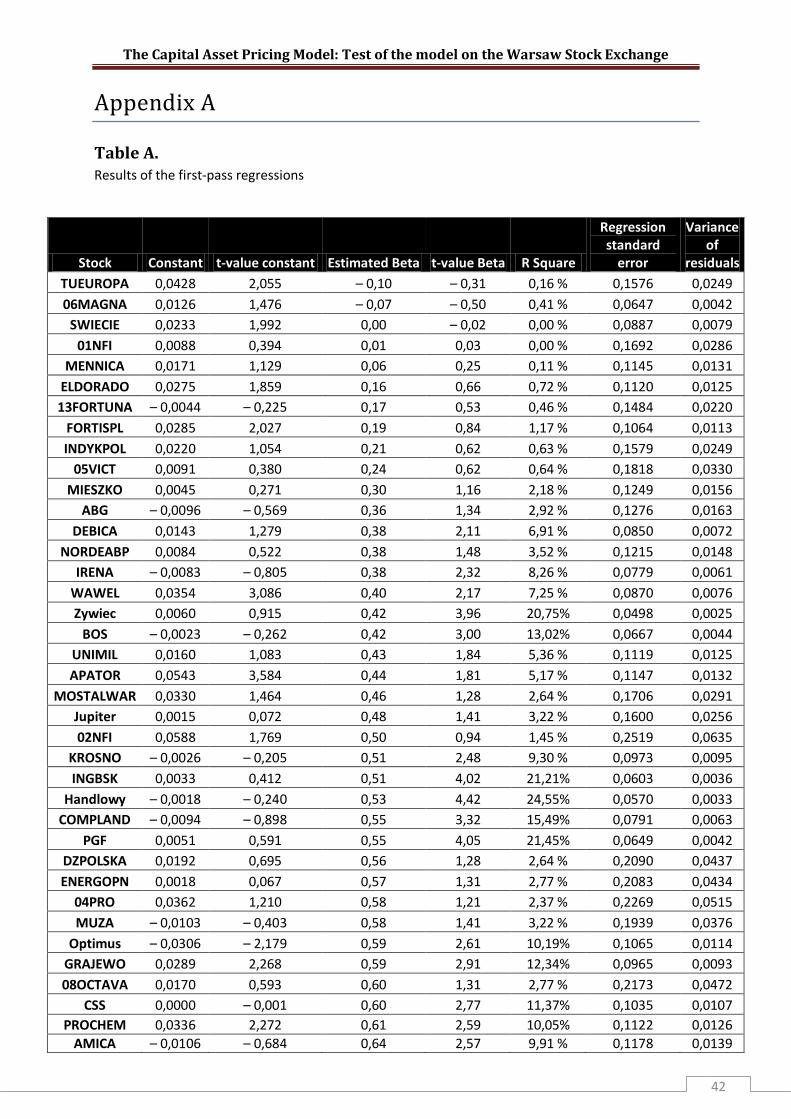
The Capital Asset Pricing Model: Test of the model on the Warsaw Stock Exchange
42
Appendix A
Table A. Results of the first-pass regressions
Stock Constant t-value constant Estimated Beta t-value Beta R Square
Regression standard
error
Variance of
residuals
TUEUROPA 0,0428 2,055 – 0,10 – 0,31 0,16 % 0,1576 0,0249
06MAGNA 0,0126 1,476 – 0,07 – 0,50 0,41 % 0,0647 0,0042
SWIECIE 0,0233 1,992 0,00 – 0,02 0,00 % 0,0887 0,0079
01NFI 0,0088 0,394 0,01 0,03 0,00 % 0,1692 0,0286
MENNICA 0,0171 1,129 0,06 0,25 0,11 % 0,1145 0,0131
ELDORADO 0,0275 1,859 0,16 0,66 0,72 % 0,1120 0,0125
13FORTUNA – 0,0044 – 0,225 0,17 0,53 0,46 % 0,1484 0,0220
FORTISPL 0,0285 2,027 0,19 0,84 1,17 % 0,1064 0,0113
INDYKPOL 0,0220 1,054 0,21 0,62 0,63 % 0,1579 0,0249
05VICT 0,0091 0,380 0,24 0,62 0,64 % 0,1818 0,0330
MIESZKO 0,0045 0,271 0,30 1,16 2,18 % 0,1249 0,0156
ABG – 0,0096 – 0,569 0,36 1,34 2,92 % 0,1276 0,0163
DEBICA 0,0143 1,279 0,38 2,11 6,91 % 0,0850 0,0072
NORDEABP 0,0084 0,522 0,38 1,48 3,52 % 0,1215 0,0148
IRENA – 0,0083 – 0,805 0,38 2,32 8,26 % 0,0779 0,0061
WAWEL 0,0354 3,086 0,40 2,17 7,25 % 0,0870 0,0076
Zywiec 0,0060 0,915 0,42 3,96 20,75% 0,0498 0,0025
BOS – 0,0023 – 0,262 0,42 3,00 13,02% 0,0667 0,0044
UNIMIL 0,0160 1,083 0,43 1,84 5,36 % 0,1119 0,0125
APATOR 0,0543 3,584 0,44 1,81 5,17 % 0,1147 0,0132
MOSTALWAR 0,0330 1,464 0,46 1,28 2,64 % 0,1706 0,0291
Jupiter 0,0015 0,072 0,48 1,41 3,22 % 0,1600 0,0256
02NFI 0,0588 1,769 0,50 0,94 1,45 % 0,2519 0,0635
KROSNO – 0,0026 – 0,205 0,51 2,48 9,30 % 0,0973 0,0095
INGBSK 0,0033 0,412 0,51 4,02 21,21% 0,0603 0,0036
Handlowy – 0,0018 – 0,240 0,53 4,42 24,55% 0,0570 0,0033
COMPLAND – 0,0094 – 0,898 0,55 3,32 15,49% 0,0791 0,0063
PGF 0,0051 0,591 0,55 4,05 21,45% 0,0649 0,0042
DZPOLSKA 0,0192 0,695 0,56 1,28 2,64 % 0,2090 0,0437
ENERGOPN 0,0018 0,067 0,57 1,31 2,77 % 0,2083 0,0434
04PRO 0,0362 1,210 0,58 1,21 2,37 % 0,2269 0,0515
MUZA – 0,0103 – 0,403 0,58 1,41 3,22 % 0,1939 0,0376
Optimus – 0,0306 – 2,179 0,59 2,61 10,19% 0,1065 0,0114
GRAJEWO 0,0289 2,268 0,59 2,91 12,34% 0,0965 0,0093
08OCTAVA 0,0170 0,593 0,60 1,31 2,77 % 0,2173 0,0472
CSS 0,0000 – 0,001 0,60 2,77 11,37% 0,1035 0,0107
PROCHEM 0,0336 2,272 0,61 2,59 10,05% 0,1122 0,0126
AMICA – 0,0106 – 0,684 0,64 2,57 9,91 % 0,1178 0,0139
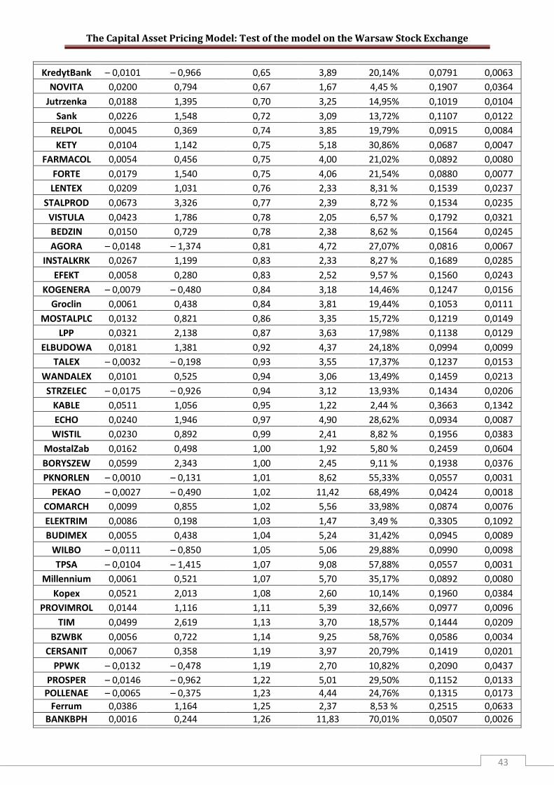
The Capital Asset Pricing Model: Test of the model on the Warsaw Stock Exchange
43
KredytBank – 0,0101 – 0,966 0,65 3,89 20,14% 0,0791 0,0063
NOVITA 0,0200 0,794 0,67 1,67 4,45 % 0,1907 0,0364
Jutrzenka 0,0188 1,395 0,70 3,25 14,95% 0,1019 0,0104
Sank 0,0226 1,548 0,72 3,09 13,72% 0,1107 0,0122
RELPOL 0,0045 0,369 0,74 3,85 19,79% 0,0915 0,0084
KETY 0,0104 1,142 0,75 5,18 30,86% 0,0687 0,0047
FARMACOL 0,0054 0,456 0,75 4,00 21,02% 0,0892 0,0080
FORTE 0,0179 1,540 0,75 4,06 21,54% 0,0880 0,0077
LENTEX 0,0209 1,031 0,76 2,33 8,31 % 0,1539 0,0237
STALPROD 0,0673 3,326 0,77 2,39 8,72 % 0,1534 0,0235
VISTULA 0,0423 1,786 0,78 2,05 6,57 % 0,1792 0,0321
BEDZIN 0,0150 0,729 0,78 2,38 8,62 % 0,1564 0,0245
AGORA – 0,0148 – 1,374 0,81 4,72 27,07% 0,0816 0,0067
INSTALKRK 0,0267 1,199 0,83 2,33 8,27 % 0,1689 0,0285
EFEKT 0,0058 0,280 0,83 2,52 9,57 % 0,1560 0,0243
KOGENERA – 0,0079 – 0,480 0,84 3,18 14,46% 0,1247 0,0156
Groclin 0,0061 0,438 0,84 3,81 19,44% 0,1053 0,0111
MOSTALPLC 0,0132 0,821 0,86 3,35 15,72% 0,1219 0,0149
LPP 0,0321 2,138 0,87 3,63 17,98% 0,1138 0,0129
ELBUDOWA 0,0181 1,381 0,92 4,37 24,18% 0,0994 0,0099
TALEX – 0,0032 – 0,198 0,93 3,55 17,37% 0,1237 0,0153
WANDALEX 0,0101 0,525 0,94 3,06 13,49% 0,1459 0,0213
STRZELEC – 0,0175 – 0,926 0,94 3,12 13,93% 0,1434 0,0206
KABLE 0,0511 1,056 0,95 1,22 2,44 % 0,3663 0,1342
ECHO 0,0240 1,946 0,97 4,90 28,62% 0,0934 0,0087
WISTIL 0,0230 0,892 0,99 2,41 8,82 % 0,1956 0,0383
MostalZab 0,0162 0,498 1,00 1,92 5,80 % 0,2459 0,0604
BORYSZEW 0,0599 2,343 1,00 2,45 9,11 % 0,1938 0,0376
PKNORLEN – 0,0010 – 0,131 1,01 8,62 55,33% 0,0557 0,0031
PEKAO – 0,0027 – 0,490 1,02 11,42 68,49% 0,0424 0,0018
COMARCH 0,0099 0,855 1,02 5,56 33,98% 0,0874 0,0076
ELEKTRIM 0,0086 0,198 1,03 1,47 3,49 % 0,3305 0,1092
BUDIMEX 0,0055 0,438 1,04 5,24 31,42% 0,0945 0,0089
WILBO – 0,0111 – 0,850 1,05 5,06 29,88% 0,0990 0,0098
TPSA – 0,0104 – 1,415 1,07 9,08 57,88% 0,0557 0,0031
Millennium 0,0061 0,521 1,07 5,70 35,17% 0,0892 0,0080
Kopex 0,0521 2,013 1,08 2,60 10,14% 0,1960 0,0384
PROVIMROL 0,0144 1,116 1,11 5,39 32,66% 0,0977 0,0096
TIM 0,0499 2,619 1,13 3,70 18,57% 0,1444 0,0209
BZWBK 0,0056 0,722 1,14 9,25 58,76% 0,0586 0,0034
CERSANIT 0,0067 0,358 1,19 3,97 20,79% 0,1419 0,0201
PPWK – 0,0132 – 0,478 1,19 2,70 10,82% 0,2090 0,0437
PROSPER – 0,0146 – 0,962 1,22 5,01 29,50% 0,1152 0,0133
POLLENAE – 0,0065 – 0,375 1,23 4,44 24,76% 0,1315 0,0173
Ferrum 0,0386 1,164 1,25 2,37 8,53 % 0,2515 0,0633
BANKBPH 0,0016 0,244 1,26 11,83 70,01% 0,0507 0,0026
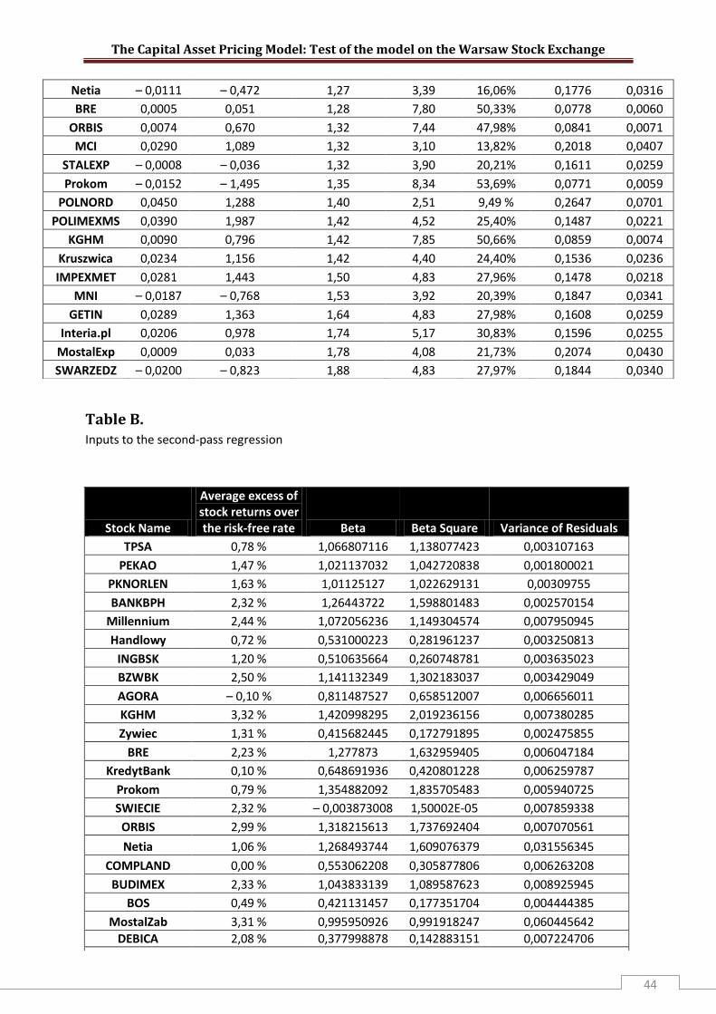
The Capital Asset Pricing Model: Test of the model on the Warsaw Stock Exchange
44
Table B. Inputs to the second-pass regression
Stock Name
Average excess of stock returns over the risk-free rate Beta Beta Square Variance of Residuals
TPSA 0,78 % 1,066807116 1,138077423 0,003107163
PEKAO 1,47 % 1,021137032 1,042720838 0,001800021
PKNORLEN 1,63 % 1,01125127 1,022629131 0,00309755
BANKBPH 2,32 % 1,26443722 1,598801483 0,002570154
Millennium 2,44 % 1,072056236 1,149304574 0,007950945
Handlowy 0,72 % 0,531000223 0,281961237 0,003250813
INGBSK 1,20 % 0,510635664 0,260748781 0,003635023
BZWBK 2,50 % 1,141132349 1,302183037 0,003429049
AGORA – 0,10 % 0,811487527 0,658512007 0,006656011
KGHM 3,32 % 1,420998295 2,019236156 0,007380285
Zywiec 1,31 % 0,415682445 0,172791895 0,002475855
BRE 2,23 % 1,277873 1,632959405 0,006047184
KredytBank 0,10 % 0,648691936 0,420801228 0,006259787
Prokom 0,79 % 1,354882092 1,835705483 0,005940725
SWIECIE 2,32 % – 0,003873008 1,50002E-05 0,007859338
ORBIS 2,99 % 1,318215613 1,737692404 0,007070561
Netia 1,06 % 1,268493744 1,609076379 0,031556345
COMPLAND 0,00 % 0,553062208 0,305877806 0,006263208
BUDIMEX 2,33 % 1,043833139 1,089587623 0,008925945
BOS 0,49 % 0,421131457 0,177351704 0,004444385
MostalZab 3,31 % 0,995950926 0,991918247 0,060445642
DEBICA 2,08 % 0,377998878 0,142883151 0,007224706
Netia – 0,0111 – 0,472 1,27 3,39 16,06% 0,1776 0,0316
BRE 0,0005 0,051 1,28 7,80 50,33% 0,0778 0,0060
ORBIS 0,0074 0,670 1,32 7,44 47,98% 0,0841 0,0071
MCI 0,0290 1,089 1,32 3,10 13,82% 0,2018 0,0407
STALEXP – 0,0008 – 0,036 1,32 3,90 20,21% 0,1611 0,0259
Prokom – 0,0152 – 1,495 1,35 8,34 53,69% 0,0771 0,0059
POLNORD 0,0450 1,288 1,40 2,51 9,49 % 0,2647 0,0701
POLIMEXMS 0,0390 1,987 1,42 4,52 25,40% 0,1487 0,0221
KGHM 0,0090 0,796 1,42 7,85 50,66% 0,0859 0,0074
Kruszwica 0,0234 1,156 1,42 4,40 24,40% 0,1536 0,0236
IMPEXMET 0,0281 1,443 1,50 4,83 27,96% 0,1478 0,0218
MNI – 0,0187 – 0,768 1,53 3,92 20,39% 0,1847 0,0341
GETIN 0,0289 1,363 1,64 4,83 27,98% 0,1608 0,0259
Interia.pl 0,0206 0,978 1,74 5,17 30,83% 0,1596 0,0255
MostalExp 0,0009 0,033 1,78 4,08 21,73% 0,2074 0,0430
SWARZEDZ – 0,0200 – 0,823 1,88 4,83 27,97% 0,1844 0,0340
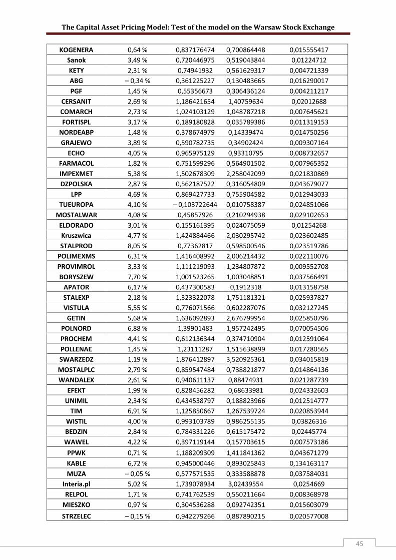
The Capital Asset Pricing Model: Test of the model on the Warsaw Stock Exchange
45
KOGENERA 0,64 % 0,837176474 0,700864448 0,015555417
Sanok 3,49 % 0,720446975 0,519043844 0,01224712
KETY 2,31 % 0,74941932 0,561629317 0,004721339
ABG – 0,34 % 0,361225227 0,130483665 0,016290017
PGF 1,45 % 0,55356673 0,306436124 0,004211217
CERSANIT 2,69 % 1,186421654 1,40759634 0,02012688
COMARCH 2,73 % 1,024103129 1,048787218 0,007645621
FORTISPL 3,17 % 0,189180828 0,035789386 0,011319153
NORDEABP 1,48 % 0,378674979 0,14339474 0,014750256
GRAJEWO 3,89 % 0,590782735 0,34902424 0,009307164
ECHO 4,05 % 0,965975129 0,93310795 0,008732657
FARMACOL 1,82 % 0,751599296 0,564901502 0,007965352
IMPEXMET 5,38 % 1,502678309 2,258042099 0,021830869
DZPOLSKA 2,87 % 0,562187522 0,316054809 0,043679077
LPP 4,69 % 0,869427733 0,755904582 0,012943033
TUEUROPA 4,10 % – 0,103722644 0,010758387 0,024851066
MOSTALWAR 4,08 % 0,45857926 0,210294938 0,029102653
ELDORADO 3,01 % 0,155161395 0,024075059 0,01254268
Kruszwica 4,77 % 1,424884466 2,030295742 0,023602485
STALPROD 8,05 % 0,77362817 0,598500546 0,023519786
POLIMEXMS 6,31 % 1,416408992 2,006214432 0,022110076
PROVIMROL 3,33 % 1,111219093 1,234807872 0,009552708
BORYSZEW 7,70 % 1,001523265 1,003048851 0,037566491
APATOR 6,17 % 0,437300583 0,1912318 0,013158758
STALEXP 2,18 % 1,323322078 1,751181321 0,025937827
VISTULA 5,55 % 0,776071566 0,602287076 0,032127245
GETIN 5,68 % 1,636092893 2,676799954 0,025850796
POLNORD 6,88 % 1,39901483 1,957242495 0,070054506
PROCHEM 4,41 % 0,612136344 0,374710904 0,012591064
POLLENAE 1,45 % 1,23111287 1,515638899 0,017280565
SWARZEDZ 1,19 % 1,876412897 3,520925361 0,034015819
MOSTALPLC 2,79 % 0,859547484 0,738821877 0,014864136
WANDALEX 2,61 % 0,940611137 0,88474931 0,021287739
EFEKT 1,99 % 0,828456282 0,68633981 0,024332603
UNIMIL 2,34 % 0,434538797 0,188823966 0,012514777
TIM 6,91 % 1,125850667 1,267539724 0,020853944
WISTIL 4,00 % 0,993103789 0,986255135 0,03826316
BEDZIN 2,84 % 0,784331226 0,615175472 0,02445774
WAWEL 4,22 % 0,397119144 0,157703615 0,007573186
PPWK 0,71 % 1,188209309 1,411841362 0,043671279
KABLE 6,72 % 0,945000446 0,893025843 0,134163117
MUZA – 0,05 % 0,577571535 0,333588878 0,037584031
Interia.pl 5,02 % 1,739078934 3,02439554 0,0254669
RELPOL 1,71 % 0,741762539 0,550211664 0,008368978
MIESZKO 0,97 % 0,304536288 0,092742351 0,015603079
STRZELEC – 0,15 % 0,942279266 0,887890215 0,020577008
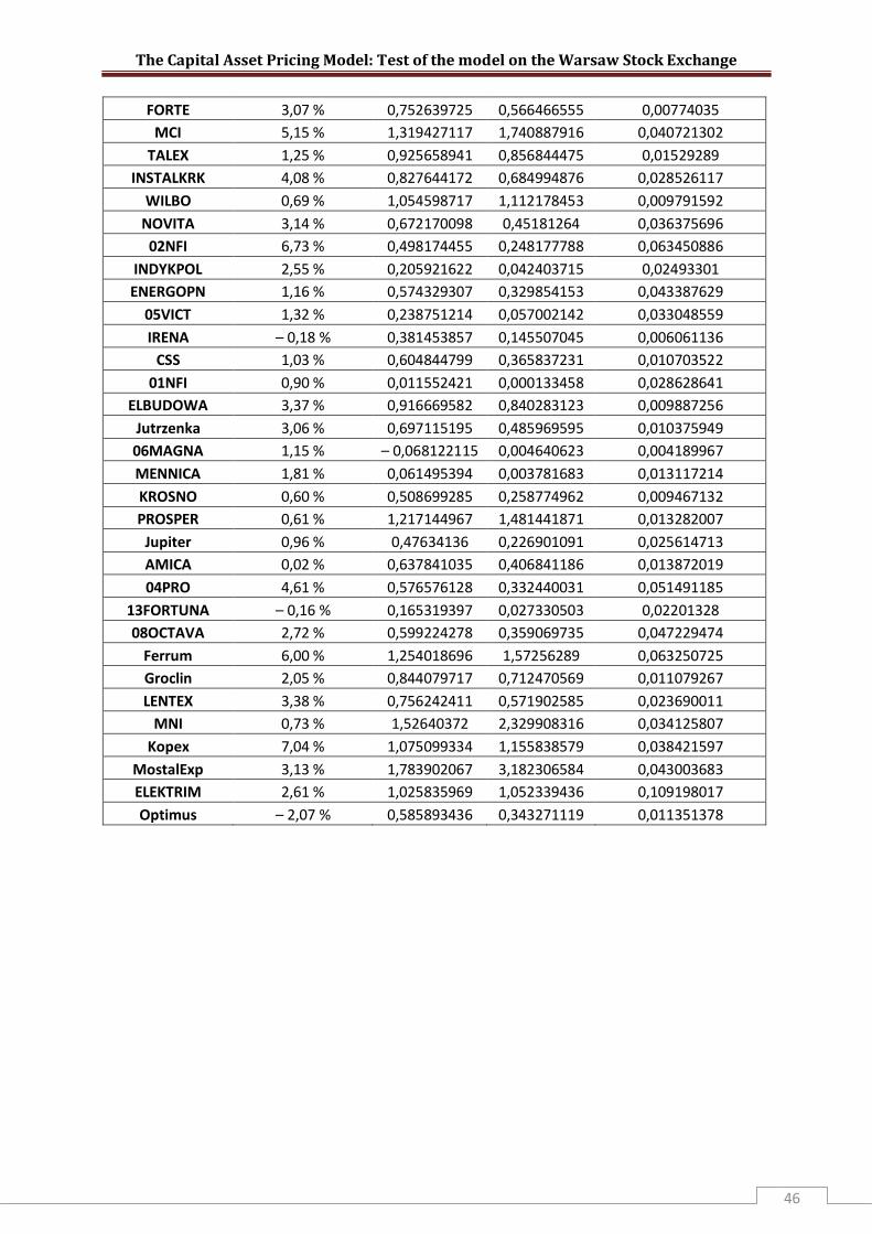
The Capital Asset Pricing Model: Test of the model on the Warsaw Stock Exchange
46
FORTE 3,07 % 0,752639725 0,566466555 0,00774035
MCI 5,15 % 1,319427117 1,740887916 0,040721302
TALEX 1,25 % 0,925658941 0,856844475 0,01529289
INSTALKRK 4,08 % 0,827644172 0,684994876 0,028526117
WILBO 0,69 % 1,054598717 1,112178453 0,009791592
NOVITA 3,14 % 0,672170098 0,45181264 0,036375696
02NFI 6,73 % 0,498174455 0,248177788 0,063450886
INDYKPOL 2,55 % 0,205921622 0,042403715 0,02493301
ENERGOPN 1,16 % 0,574329307 0,329854153 0,043387629
05VICT 1,32 % 0,238751214 0,057002142 0,033048559
IRENA – 0,18 % 0,381453857 0,145507045 0,006061136
CSS 1,03 % 0,604844799 0,365837231 0,010703522
01NFI 0,90 % 0,011552421 0,000133458 0,028628641
ELBUDOWA 3,37 % 0,916669582 0,840283123 0,009887256
Jutrzenka 3,06 % 0,697115195 0,485969595 0,010375949
06MAGNA 1,15 % – 0,068122115 0,004640623 0,004189967
MENNICA 1,81 % 0,061495394 0,003781683 0,013117214
KROSNO 0,60 % 0,508699285 0,258774962 0,009467132
PROSPER 0,61 % 1,217144967 1,481441871 0,013282007
Jupiter 0,96 % 0,47634136 0,226901091 0,025614713
AMICA 0,02 % 0,637841035 0,406841186 0,013872019
04PRO 4,61 % 0,576576128 0,332440031 0,051491185
13FORTUNA – 0,16 % 0,165319397 0,027330503 0,02201328
08OCTAVA 2,72 % 0,599224278 0,359069735 0,047229474
Ferrum 6,00 % 1,254018696 1,57256289 0,063250725
Groclin 2,05 % 0,844079717 0,712470569 0,011079267
LENTEX 3,38 % 0,756242411 0,571902585 0,023690011
MNI 0,73 % 1,52640372 2,329908316 0,034125807
Kopex 7,04 % 1,075099334 1,155838579 0,038421597
MostalExp 3,13 % 1,783902067 3,182306584 0,043003683
ELEKTRIM 2,61 % 1,025835969 1,052339436 0,109198017
Optimus – 2,07 % 0,585893436 0,343271119 0,011351378
freeee

The Capital Asset Pricing Model: Test of the model on the Warsaw Stock Exchange
47
Appendix B
Table A. Estimated stocks’ betas in years 2002-2003
Stock Name Intercept t-value Intercept Beta t-value Beta R-Square Regressions Standard Error
06MAGNA 0,00557532 0,477773581 -0,35713 -2,359383028 20,19% 0,056209535
SWIECIE 0,04837366 2,56376462 -0,21238 -0,867746282 3,31% 0,090885183
INDYKPOL -0,0083785 -0,427014147 -0,11145 -0,437891964 0,86% 0,094512092
ABG 0,01760185 0,615374952 -0,09412 -0,253671164 0,29% 0,137778261
MOSTALWAR 0,02239953 0,956180025 -0,00674 -0,022194203 0,00% 0,112839591
13FORTUNA -0,0120073 -0,997880264 0,016271 0,104246494 0,05% 0,057960347
08OCTAVA 0,03896732 0,802853307 0,032892 0,052245243 0,01% 0,233790349
MIESZKO 0,00271491 0,200938542 0,038992 0,2224827 0,22% 0,065080986
05VICT 0,00446355 0,25954491 0,053908 0,241658392 0,26% 0,08283804
01NFI 0,0009608 0,083960296 0,104489 0,703925698 2,20% 0,05512181
04PRO -0,0107487 -0,788572372 0,107535 0,608210489 1,65% 0,065656236
FORTISPL 0,04618648 1,707217426 0,115111 0,328026125 0,49% 0,130313158
UNIMIL 0,04425335 1,727327356 0,119246 0,358831033 0,58% 0,123405278
APATOR 0,07564299 2,563602377 0,14488 0,378535039 0,65% 0,142128209
02NFI 0,01050399 0,52467696 0,145875 0,561741711 1,41% 0,096432774
Jupiter -0,0310636 -2,006195714 0,171432 0,853551781 3,21% 0,07458319
TUEUROPA 0,00671589 0,33125144 0,198972 0,756594938 2,54% 0,097658025
MUZA -0,0326303 -0,889272935 0,244348 0,513380464 1,18% 0,176745693
ENERGOPN -0,0256893 -0,411421987 0,266323 0,328822084 0,49% 0,300764413
INGBSK -0,0035632 -0,236906876 0,328487 1,683741858 11,42% 0,072447183
MENNICA -0,0133148 -0,72948797 0,393807 1,663352356 11,17% 0,087918078
KredytBank -0,0420972 -2,580045749 0,396111 1,871580292 13,74% 0,078593714
BOS -0,0101984 -0,650011956 0,409238 2,010866646 15,53% 0,075574022
IRENA -0,0054757 -0,321340765 0,411179 1,860272489 13,59% 0,082079244
MostalZab -0,0480682 -0,994660593 0,444439 0,708999862 2,23% 0,232779973
AMICA -0,009203 -0,366751451 0,492555 1,513263593 9,43% 0,120870392
NORDEABP 0,01486785 0,480672549 0,493443 1,229859342 6,43% 0,148991373
Optimus -0,0330435 -1,298098341 0,513813 1,556122796 9,92% 0,122614231
WAWEL 0,01825942 1,178317457 0,554506 2,758664411 25,70% 0,074642632
STRZELEC -0,0168426 -0,639780464 0,570652 1,671133764 11,26% 0,126805802
ELDORADO 0,01974307 1,212638738 0,576416 2,729417916 25,30% 0,078423386
Handlowy -0,0134269 -1,122066542 0,58258 3,753318239 39,04% 0,057639455
POLNORD -0,0155881 -0,654779314 0,585155 1,894914562 14,03% 0,114672895
GRAJEWO 0,04381201 1,557831411 0,604115 1,656014731 11,08% 0,135467463
PROCHEM 0,00786554 0,454904112 0,612163 2,729454919 25,30% 0,083285773
NOVITA -0,0268547 -0,688834272 0,613008 1,212210739 6,26% 0,187787748
CSS -0,0181948 -0,751013092 0,62831 1,999363351 15,38% 0,11669755
MOSTALPLC -0,0135991 -1,213042443 0,630397 4,335070789 46,07% 0,054000404
Zywiec 0,01754328 1,327349144 0,635086 3,704454263 38,41% 0,063663127

The Capital Asset Pricing Model: Test of the model on the Warsaw Stock Exchange
48
Kopex 0,07046021 1,448979325 0,694345 1,100806464 5,22% 0,23423081
PGF 0,00052356 0,037756644 0,695767 3,868188586 40,48% 0,066793735
COMPLAND -0,0160206 -0,886681142 0,70395 3,003631125 29,08% 0,087031145
DZPOLSKA -0,0228277 -0,749421414 0,7105 1,798233342 12,81% 0,146722802
ELBUDOWA -0,0145036 -0,814857276 0,718448 3,111842473 30,56% 0,085734809
DEBICA 0,0501957 3,966818669 0,72798 4,435194421 47,21% 0,060951788
INSTALKRK -0,0155296 -0,385394162 0,72919 1,39508839 8,13% 0,194096721
KROSNO 0,0173813 0,817015927 0,735526 2,665405211 24,41% 0,102474067
EFEKT -0,0397053 -1,205158061 0,750577 1,756337983 12,30% 0,158696258
FORTE 0,05114381 2,394636755 0,782058 2,822946682 26,59% 0,102876382
FARMACOL 0,01624264 0,616556919 0,789847 2,311408672 19,54% 0,12689536
ECHO 0,01498965 0,81431305 0,825627 3,457807868 35,21% 0,088667062
KETY 0,03405852 2,333996076 0,838511 4,429965666 47,15% 0,070289085
STALPROD 0,03110743 1,124880148 0,843924 2,352678574 20,10% 0,133204864
PKNORLEN 0,00554079 0,470743604 0,857556 5,6168453 58,92% 0,056695597
Millennium -0,0157355 -0,86172866 0,872324 3,682868995 38,14% 0,087957139
VISTULA -0,0038037 -0,079222541 0,899844 1,444862982 8,67% 0,231270311
PEKAO -0,0087108 -0,904751672 0,911019 7,294841777 70,75% 0,046375735
WANDALEX -0,0046676 -0,140118717 0,916837 2,121839105 16,99% 0,16045716
BZWBK 0,00323209 0,290774148 0,923973 6,408394582 65,12% 0,053541372
CERSANIT -0,0181795 -0,450845127 0,926575 1,771509234 12,48% 0,194230134
Groclin 0,06523062 3,181623874 0,927042 3,485889738 35,58% 0,098756322
LPP 0,08288062 3,083925225 0,937118 2,68820513 24,73% 0,129452792
BEDZIN 0,06035558 1,386868133 0,937418 1,66061213 11,14% 0,209625682
AGORA -0,0063962 -0,39226719 0,950881 4,495771266 47,88% 0,07854189
RELPOL 0,01016489 0,544033474 0,955428 3,942191652 41,40% 0,08999938
KOGENERA -0,03392 -1,218274482 0,967392 2,678608709 24,59% 0,134113484
LENTEX 0,00756476 0,35858497 0,986262 3,604181407 37,13% 0,101616702
TPSA -0,0114564 -0,870692717 1,035187 6,065323239 62,58% 0,063378814
Sanok 0,05045679 1,862876523 1,073967 3,056838016 29,81% 0,130466147
Jutrzenka 0,00898665 0,594372168 1,077771 5,495458029 57,85% 0,072828577
TALEX 0,01889623 0,698333382 1,099022 3,131203635 30,83% 0,130339062
WILBO -0,0149071 -0,852542478 1,126524 4,966857061 52,86% 0,084224428
BUDIMEX -0,0003591 -0,026710222 1,143863 6,558534094 66,16% 0,064765904
ELEKTRIM -0,0454936 -1,251935919 1,186031 2,516198326 22,35% 0,175037296
Ferrum 0,02052366 0,355216814 1,196658 1,596709847 10,39% 0,278306574
COMARCH -0,0071511 -0,433811056 1,238731 5,793209134 60,40% 0,07940307
PPWK -0,0531767 -1,297815692 1,25537 2,362001978 20,23% 0,197365271
BANKBPH 0,00137457 0,099766499 1,291887 7,228702294 70,37% 0,066365707
PROVIMROL 0,04300335 2,052298455 1,315758 4,840958513 51,58% 0,100930867
KGHM 0,01954785 1,212122621 1,331276 6,364038561 64,80% 0,077680982
Prokom 0,00444901 0,262483053 1,344235 6,114069475 62,95% 0,081643981
BRE -0,0210396 -1,008358316 1,346387 4,974676659 52,94% 0,100504237
TIM 0,01850671 0,638634917 1,372733 3,651965024 37,74% 0,139585033
MostalExp -0,0373688 -0,974535258 1,399442 2,813590041 26,46% 0,184702771
MCI -0,0156977 -0,495193571 1,44359 3,510742593 35,91% 0,152694805

The Capital Asset Pricing Model: Test of the model on the Warsaw Stock Exchange
49
PROSPER -0,0097629 -0,334172494 1,52825 4,032770974 42,50% 0,140724698
BORYSZEW 0,11805953 2,44632209 1,537917 2,456759907 21,53% 0,232460772
POLLENAE -0,0102319 -0,337492818 1,60607 4,084039741 43,12% 0,146034003
STALEXP -0,0254055 -0,853897985 1,624344 4,208953202 44,61% 0,143312278
ORBIS 0,00246263 0,134697806 1,636691 6,901521391 68,40% 0,088064575
MNI -0,0851334 -1,607756085 1,71336 2,494512688 22,05% 0,255059901
SWARZEDZ -0,0296098 -0,800689875 1,760399 3,669924346 37,97% 0,178128479
Interia.pl 0,00638962 0,202436448 1,766368 4,314313074 45,83% 0,152036847
WISTIL 0,09238486 1,785445987 1,772635 2,641084612 24,07% 0,249239182
IMPEXMET 0,02657942 0,774512592 1,909953 4,290648467 45,56% 0,165302422
Netia -0,0091304 -0,168531945 1,936732 2,756007853 25,66% 0,260956692
POLIMEXMS 0,00705509 0,223106946 2,003782 4,885151662 52,03% 0,152318204
GETIN 0,01846817 0,408285712 2,060134 3,51117895 35,91% 0,217882249
Kruszwica 0,05311032 1,419785422 2,254531 4,646405654 49,53% 0,180184912
KABLE -0,0023689 -0,05321078 2,26787 3,927287322 41,21% 0,214439542
Table B. Estimated stocks’ betas in years 2003-2004
Stock Name Intercept t-value Intercept Beta t-value Beta R-Square Regressions
Standard Error
TPSA -0,00334187 -0,28427001 0,895181 4,758102369 50,72% 0,053668499
PEKAO -0,00593836 -0,726365967 0,995014 7,605012971 72,44% 0,037322546
PKNORLEN 0,01225198 1,567111903 0,784437 6,269508325 64,11% 0,035691667
BANKBPH -0,00191009 -0,164668703 1,201688 6,47335845 65,57% 0,052954694
Millennium -0,01299491 -0,738365661 0,565912 2,009224408 15,50% 0,080345647
Handlowy -0,021303 -1,624478352 0,858544 4,090888159 43,20% 0,059866979
INGBSK -0,01045501 -0,633320752 0,418615 1,584512662 10,24% 0,075363532
BZWBK -0,01018581 -1,285100433 0,943437 7,437658567 71,55% 0,036184191
AGORA -0,01943466 -1,255303032 1,092265 4,408401919 46,90% 0,070678778
KGHM 0,01245547 0,727210014 1,350756 4,927859036 52,47% 0,078191729
Zywiec -0,00581457 -0,494268531 0,574164 3,049741834 29,71% 0,053705079
BRE -0,01754422 -0,9929321 1,30663 4,620828307 49,25% 0,080663119
KredytBank -0,03945158 -2,392483802 0,767684 2,909035092 27,78% 0,075279362
Prokom -0,02254681 -1,386702251 1,279174 4,915972886 52,35% 0,074227107
SWIECIE 0,04051878 1,83620426 -0,56356 -1,595831845 10,37% 0,100738606
ORBIS -0,01685891 -1,002030147 1,575994 5,853123052 60,90% 0,076808476
Netia -0,01041311 -0,717260533 1,098666 4,728721718 50,41% 0,066277222
COMPLAND -0,00317264 -0,169833501 0,475452 1,590343037 10,31% 0,085282103
BUDIMEX -0,01209066 -0,742108985 1,143258 4,384739297 46,64% 0,074377703
BOS -0,01315534 -1,236708034 0,3282 1,927902038 14,45% 0,048561865
MostalZab -0,0192085 -0,418939719 0,676089 0,921390876 3,72% 0,209315974
DEBICA 0,02005032 1,248902292 0,604018 2,350924377 20,08% 0,073291483
KOGENERA 0,02913282 1,142143339 0,944086 2,312763581 19,56% 0,116445433
Sanok 0,03439219 1,242648119 1,656818 3,740630851 38,88% 0,126349111
KETY 0,01715928 1,072529593 1,060551 4,142126611 43,82% 0,073038246

The Capital Asset Pricing Model: Test of the model on the Warsaw Stock Exchange
50
ABG -0,00453459 -0,121461404 0,155724 0,260637703 0,31% 0,170435525
PGF 0,01187079 0,937774254 0,865582 4,272762228 45,35% 0,057788558
CERSANIT 0,0166099 1,734889693 1,029645 6,720074389 67,24% 0,043707471
COMARCH 0,01716069 1,135043903 1,113791 4,603237122 49,06% 0,069021206
FORTISPL 0,03023027 1,364816088 0,408604 1,152699862 5,70% 0,101118
NORDEABP 0,0009145 0,030679992 1,008856 2,114854716 16,90% 0,136078957
GRAJEWO 0,04207938 1,537140556 1,018125 2,323951082 19,71% 0,124973049
ECHO 0,00134987 0,107095357 1,493264 7,402836437 71,35% 0,057541453
FARMACOL 0,01857239 0,661986013 0,580989 1,2939887 7,07% 0,128079461
IMPEXMET 0,0547986 1,734540679 1,683002 3,328751607 33,50% 0,144226663
DZPOLSKA -0,00443791 -0,162610825 -0,08304 -0,19012729 0,16% 0,124591766
LPP 0,02419395 1,00441171 0,961607 2,494505883 22,05% 0,109965258
TUEUROPA 0,04147611 0,873844265 0,087137 0,114714977 0,06% 0,216682828
MOSTALWAR -0,00421088 -0,129513706 0,122955 0,236304452 0,25% 0,148428661
ELDORADO 0,0189709 1,463195622 1,030262 4,965281715 52,84% 0,059189706
Kruszwica 0,02929921 0,795228131 3,089048 5,238925083 55,51% 0,16819952
STALPROD 0,05251235 1,709676688 1,491611 3,034518533 29,51% 0,140219376
POLIMEXMS 0,04832486 1,10956944 2,38466 3,421306207 34,73% 0,198827619
PROVIMROL 0,01277994 0,682874066 1,975318 6,595241832 66,41% 0,085437518
BORYSZEW 0,11196461 2,201327889 2,418233 2,970870747 28,63% 0,232196998
APATOR 0,07450046 2,73858811 0,288243 0,662076861 1,95% 0,124191762
STALEXP 0,00603471 0,179193542 1,470407 2,728256972 25,28% 0,153742681
VISTULA 0,11902179 2,351547159 0,761507 0,940119053 3,86% 0,231064566
GETIN 0,05194245 1,305056709 1,456096 2,28601281 19,19% 0,181699465
POLNORD -0,02002534 -0,685013754 0,995175 2,127160872 17,06% 0,133456956
PROCHEM 0,03910985 1,16349633 0,912015 1,695362333 11,56% 0,153455225
POLLENAE 0,00713114 0,233848293 2,28774 4,687740137 49,97% 0,13921482
SWARZEDZ 0,02452178 0,462689668 2,000322 2,358410362 20,18% 0,241948416
MOSTALPLC 0,01395676 0,529576901 0,632039 1,498546491 9,26% 0,120314001
WANDALEX 0,02772858 0,700808497 0,816715 1,289805185 7,03% 0,180629561
EFEKT 0,01204844 0,485439102 1,151826 2,899829173 27,65% 0,113307006
UNIMIL 0,00580493 0,215971566 0,210482 0,489323463 1,08% 0,122704685
TIM 0,11559058 2,96996886 1,173861 1,884637975 13,90% 0,177676963
WISTIL 0,03938937 0,860839468 3,17881 4,340995805 46,14% 0,208889873
BEDZIN 0,04486702 1,214762525 1,492508 2,52500595 22,47% 0,168615085
WAWEL 0,05330277 3,140313934 0,568988 2,094633568 16,63% 0,077488508
PPWK 0,0116447 0,359556784 1,20272 2,320519553 19,66% 0,147850074
KABLE 0,05603673 0,974873856 2,576796 2,801156084 26,29% 0,26241275
MUZA 0,00302215 0,084188414 0,371835 0,647244639 1,87% 0,163879111
Interia.pl 0,01379732 0,379339741 2,1977 3,775579035 39,32% 0,166045472
RELPOL 0,01807594 1,14557224 1,31052 5,189755681 55,04% 0,072034225
MIESZKO 0,02512372 0,647041578 -0,21529 -0,346465639 0,54% 0,177260628
STRZELEC -0,03593349 -1,156454391 1,094051 2,200130133 18,03% 0,141850677
FORTE 0,02763113 1,444168634 1,280515 4,182015753 44,29% 0,087345647
MCI 0,0581785 0,979079245 1,691976 1,779226328 12,58% 0,271272185
TALEX 0,00467348 0,166055385 0,692324 1,537104705 9,70% 0,128483673

The Capital Asset Pricing Model: Test of the model on the Warsaw Stock Exchange
51
INSTALKRK 0,02132924 0,607791374 1,008942 1,796498812 12,79% 0,160206939
WILBO -0,0152632 -0,707658195 1,294234 3,74949082 38,99% 0,098465177
NOVITA -0,00448294 -0,113568758 1,395827 2,209575748 18,16% 0,180204244
02NFI 0,03421448 1,496473207 0,484659 1,324575146 7,39% 0,104376219
INDYKPOL 0,05163745 1,096638701 0,293228 0,389122235 0,68% 0,214962048
ENERGOPN 0,03170855 0,518398856 0,341556 0,348924151 0,55% 0,279236976
05VICT 0,06830928 2,556235123 -0,06725 -0,1572479 0,11% 0,121994285
IRENA -0,00890995 -0,529993955 0,670272 2,491312836 22,00% 0,07674763
CSS -4,0516E-05 -0,003774193 0,701763 4,084743104 43,13% 0,049008141
01NFI 0,05387784 1,911177696 -0,07211 -0,15983473 0,12% 0,12869736
ELBUDOWA 0,01272171 0,483136166 0,918109 2,178711539 17,75% 0,120208874
Jutrzenka 0,01504774 0,869645489 1,032387 3,72816376 38,72% 0,078993199
06MAGNA 0,01278813 1,534722069 -0,08286 -0,621350207 1,72% 0,038039778
MENNICA 0,05706625 1,613968955 0,103378 0,182695381 0,15% 0,161415314
KROSNO 0,03129317 1,334836338 0,916795 2,443611721 21,35% 0,107024213
PROSPER 0,00476667 0,184993837 1,682573 4,080351567 43,08% 0,117630114
Jupiter -0,00093946 -0,041221118 0,180827 0,495774543 1,10% 0,104044849
AMICA -0,01337441 -0,449051499 0,734872 1,541753823 9,75% 0,135968712
04PRO 0,02744566 1,172970788 0,259414 0,692769878 2,13% 0,106818647
13FORTUNA 0,03094769 1,125388825 -0,15239 -0,346263328 0,54% 0,12554116
08OCTAVA 0,02956697 0,561170941 -0,00877 -0,010402793 0,00% 0,240531669
Ferrum 0,08949351 1,498303296 1,821445 1,90548673 14,17% 0,272679417
Groclin 0,00409295 0,251054777 0,760206 2,913703416 27,84% 0,074426619
LENTEX 0,00670479 0,31335325 0,880257 2,570635371 23,10% 0,097681263
MNI 0,04292678 0,977095098 0,95725 1,361493042 7,77% 0,200563589
Kopex 0,05222206 1,138777319 0,949339 1,293563759 7,07% 0,209351352
MostalExp -0,01224054 -0,45349808 0,883359 2,045002712 15,97% 0,123221289
ELEKTRIM 0,04022567 1,000713289 0,807654 1,255490285 6,69% 0,183507636
Optimus 0,00066385 0,032103348 0,707452 2,137761136 17,20% 0,094401807
Table C. Estimated stocks’ betas in years 2004-2005
Stock Name Intercept t-value Intercept Beta t-value Beta R-Square
Regressions Standard
Error
TPSA -0,0102075 -0,912340514 1,489877 5,959140371 61,75% 0,049831313
PEKAO -0,0041213 -0,488708798 1,357816 7,205338512 70,24% 0,037559716
PKNORLEN 0,01520069 1,510973728 1,286884 5,724356988 59,83% 0,044807255
BANKBPH 0,00738026 0,829024764 1,24333 6,249946517 63,97% 0,039650245
Millennium 0,00528098 0,350499525 1,503912 4,466724798 47,56% 0,067107148
Handlowy 0,0067192 0,536155871 0,469856 1,677767813 11,34% 0,055817234
INGBSK 0,0036159 0,319608442 0,741448 2,932763877 28,11% 0,050389442
BZWBK -0,0025889 -0,281875049 1,503638 7,326119665 70,93% 0,040907694
AGORA 0,00099003 0,063185901 0,517924 1,479219111 9,05% 0,069786111
KGHM -0,0031455 -0,168085293 1,520087 3,6350084 37,52% 0,08334866

The Capital Asset Pricing Model: Test of the model on the Warsaw Stock Exchange
52
Zywiec 0,00421609 0,628865336 0,013937 0,093029355 0,04% 0,02986027
BRE 0,00546251 0,482304638 0,955364 3,774782309 39,31% 0,050444375
KredytBank -0,0026807 -0,215985317 1,204505 4,342902383 46,16% 0,055279511
Prokom -0,0383682 -2,320245064 1,545452 4,182266284 44,29% 0,07365116
SWIECIE -0,0197872 -1,530992594 0,020819 0,072084598 0,02% 0,057564194
ORBIS -0,004788 -0,3365445 0,564144 1,774469425 12,52% 0,063366124
Netia 0,00234148 0,173138058 0,785237 2,598345012 23,48% 0,060233719
COMPLAND -0,0144481 -0,908409038 0,715818 2,01403541 15,57% 0,070838796
BUDIMEX -0,0035722 -0,177279444 0,237326 0,527065135 1,25% 0,089746407
BOS -3,254E-06 -0,000216908 0,582399 1,737260965 12,06% 0,066817649
MostalZab 0,00729509 0,161226825 1,415962 1,400398978 8,18% 0,201527969
DEBICA -0,0221741 -1,721652204 -0,17305 -0,601247069 1,62% 0,057364507
KOGENERA 0,02609041 0,855901881 0,382866 0,562061328 1,42% 0,13576845
Sanok 0,00856561 0,448983926 -0,03388 -0,079475077 0,03% 0,084970789
KETY -0,01351 -0,953569814 0,551461 1,741829546 12,12% 0,063102232
ABG -0,0437031 -1,540229767 1,098174 1,731962073 12,00% 0,126377168
PGF 0,0085248 0,6953241 0,375208 1,369523404 7,86% 0,054605781
CERSANIT 0,00786171 0,78617711 0,770737 3,44908196 35,10% 0,044538803
COMARCH -0,002868 -0,214669392 0,496893 1,664344292 11,18% 0,059505303
FORTISPL 0,01596836 0,894613751 0,867858 2,175793795 17,71% 0,079499889
NORDEABP -0,0058064 -0,243787992 0,486878 0,914788967 3,66% 0,106080377
GRAJEWO 0,02099942 1,30521091 0,255841 0,711603199 2,25% 0,071658633
ECHO 0,02306485 1,400915549 0,551916 1,500126652 9,28% 0,073329827
FARMACOL 0,00679678 0,537114717 0,662436 2,342615701 19,96% 0,056360939
IMPEXMET 0,02077546 0,830345831 0,426594 0,76298673 2,58% 0,111438055
DZPOLSKA -0,0011622 -0,040168916 0,05883 0,090988593 0,04% 0,128868524
LPP 0,01111206 0,674831907 0,057526 0,156335983 0,11% 0,073340011
TUEUROPA 0,09718778 2,003436853 -1,47353 -1,359303271 7,75% 0,216061761
MOSTALWAR -0,0245643 -0,706598429 1,356995 1,746788928 12,18% 0,154836565
ELDORADO -0,0031215 -0,228181593 0,087942 0,287681773 0,37% 0,060928321
Kruszwica -0,0001299 -0,006642652 -0,17542 -0,401286408 0,73% 0,087127074
STALPROD 0,04740871 1,569423816 0,298716 0,442521238 0,88% 0,134542591
POLIMEXMS 0,0784675 2,098704651 0,174183 0,208478076 0,20% 0,166525371
PROVIMROL -0,0229635 -1,290921225 1,789447 4,501667018 47,95% 0,079228437
BORYSZEW 0,04602622 1,352900011 0,71496 0,940450886 3,86% 0,151524024
APATOR 0,04080896 2,05758587 1,368267 3,087217348 30,23% 0,08833635
STALEXP -0,0159632 -0,548246876 0,785935 1,20791611 6,22% 0,129683709
VISTULA 0,07888854 2,380053818 0,650805 0,87865282 3,39% 0,147628112
GETIN 0,04364144 1,460835902 0,968121 1,450192183 8,73% 0,133057557
POLNORD -0,0070226 -0,209796125 0,858431 1,147616931 5,65% 0,149088549
PROCHEM 0,05190024 1,541970876 0,48697 0,647444758 1,87% 0,149911559
POLLENAE -0,0045963 -0,201413328 0,252034 0,494235343 1,10% 0,101638979
SWARZEDZ -0,0348761 -0,69508096 3,399282 3,031714971 29,47% 0,223477839
MOSTALPLC 0,04284307 1,282846175 0,141266 0,189289558 0,16% 0,148746897
WANDALEX 0,00835192 0,274916116 0,585698 0,862743382 3,27% 0,135309435
EFEKT 0,01047602 0,39859894 0,840618 1,431306146 8,52% 0,117058224

The Capital Asset Pricing Model: Test of the model on the Warsaw Stock Exchange
53
UNIMIL -0,0337471 -1,62863489 1,18124 2,551050609 22,83% 0,092289983
TIM 0,08336138 2,156686048 0,553891 0,641268615 1,83% 0,172155093
WISTIL -0,0036424 -0,13774904 -0,73144 -1,237858487 6,51% 0,117772372
BEDZIN -0,0310747 -1,491654371 0,798627 1,715531488 11,80% 0,092785737
WAWEL 0,05522293 2,879041884 -0,02667 -0,0622288 0,02% 0,085430584
PPWK 0,04532344 1,155102377 -0,47474 -0,54143276 1,31% 0,174760915
KABLE 0,02440859 0,463188959 0,180229 0,153050585 0,11% 0,234707186
MUZA -0,0048775 -0,163410364 -0,33205 -0,497832426 1,11% 0,132940148
Interia.pl 0,00561603 0,151299775 2,029212 2,446412498 21,39% 0,165323022
RELPOL -0,0079747 -0,488322094 -0,00936 -0,025646367 0,00% 0,072736436
MIESZKO 0,01646029 0,401244896 0,081319 0,088707439 0,04% 0,182713225
STRZELEC -0,0704774 -2,961827336 2,289097 4,304946706 45,72% 0,105982014
FORTE -0,0012281 -0,083254858 1,008072 3,058072872 29,83% 0,065702152
MCI 0,02292415 0,397232716 1,760044 1,364799829 7,81% 0,257033731
TALEX -0,0094474 -0,34510768 0,168029 0,274676782 0,34% 0,121926487
INSTALKRK -0,0067834 -0,287695504 1,462654 2,775994935 25,94% 0,10501672
WILBO -0,0381645 -1,69342127 1,228228 2,438812926 21,28% 0,100377489
NOVITA 0,00111791 0,032865572 0,417162 0,548822935 1,35% 0,151498419
02NFI 0,05556575 2,482796469 0,129318 0,258574768 0,30% 0,099679994
INDYKPOL 0,0363811 0,73006957 1,069282 0,960228336 4,02% 0,221949167
ENERGOPN -0,0016685 -0,060572802 1,255273 2,039295345 15,90% 0,122685635
05VICT 0,08597334 2,029522872 -1,27646 -1,348436518 7,63% 0,188673863
IRENA -0,0144675 -1,07675117 -0,1506 -0,501581883 1,13% 0,05984374
CSS -0,0215737 -1,720311665 0,885766 3,160782754 31,23% 0,055854727
01NFI 0,02714514 0,545724364 -0,2729 -0,245513994 0,27% 0,221544319
ELBUDOWA 0,01065248 0,419742577 1,483978 2,616698068 23,74% 0,113034108
Jutrzenka 0,03318948 1,176966425 0,578765 0,918458429 3,69% 0,1255967
06MAGNA 0,01576881 1,226797136 -0,23258 -0,80974428 2,89% 0,057249005
MENNICA 0,06216976 1,84180358 -0,94941 -1,258662798 6,72% 0,150341123
KROSNO 0,00674077 0,319378632 -0,2825 -0,598977644 1,60% 0,094003895
PROSPER -0,0383572 -2,38357467 1,006052 2,797671532 26,24% 0,071673657
Jupiter 0,02315263 0,809587658 -0,71374 -1,116850041 5,37% 0,127373278
AMICA -0,0225956 -0,948343412 0,654428 1,229125751 6,43% 0,106120907
04PRO 0,05573042 2,277918553 0,308282 0,563881848 1,42% 0,108967261
13FORTUNA 0,00503047 0,124125246 0,830989 0,917572878 3,69% 0,180505512
08OCTAVA -0,0014219 -0,074200556 -0,03679 -0,085907867 0,03% 0,085349862
Ferrum 0,02748947 0,667975495 1,202082 1,307139139 7,21% 0,183293812
Groclin -0,027909 -1,397535033 0,467792 1,048250156 4,76% 0,088945425
LENTEX -0,0319421 -1,458923933 0,61936 1,265920371 6,79% 0,097515289
MNI 0,02278866 0,958185777 1,008713 1,897983023 14,07% 0,105928054
Kopex -0,0163809 -0,887679986 1,304678 3,163842315 31,27% 0,082191001
MostalExp -0,0118077 -0,551569689 1,45501 3,041561194 29,60% 0,095346589
ELEKTRIM -0,0018781 -0,044462994 0,649462 0,688062032 2,11% 0,188131647
Optimus -0,0228697 -1,060672231 0,85693 1,778528347 12,57% 0,096032948

The Capital Asset Pricing Model: Test of the model on the Warsaw Stock Exchange
54
Table D Estimated portfolios’ betas
Portfolio Intercept t-value Intercept Beta t-value Beta R-Square
Regressions Standard
Error
1 0,00711128 0,586059139 0,567484 2,366031708 14,14% 0,066802062
2 0,02119043 2,810924083 0,628821 4,219971712 34,37% 0,041502513
3 0,03073911 2,306986866 0,563046 2,137818999 11,85% 0,073355029
4 0,01204183 1,074322935 0,731949 3,303668679 24,30% 0,061708006
5 0,0061135 0,846217867 0,799905 5,601491311 47,99% 0,039773299
6 0,03223986 3,13327202 0,649953 3,195656202 23,10% 0,056647247
7 0,01023921 0,814962804 0,806912 3,249159847 23,69% 0,069169129
8 0,01413547 1,44545781 0,834141 4,315267428 35,39% 0,053837948
9 0,02509914 2,193205355 1,010285 4,466194711 36,98% 0,06300328
10 0,00856639 0,760101037 0,864074 3,878804099 30,68% 0,062045454

The Capital Asset Pricing Model: Test of the model on the Warsaw Stock Exchange
55
Appendix C
Table A Estimated stocks’ betas in years 2002-2003
Stock Name Intercept t-value Intercept Beta t-value Beta R-Square Regressions
Standard Error
06MAGNA 0,00557532 0,477773581 -0,35713 -2,359383028 20,19% 0,056209535
SWIECIE 0,04837366 2,56376462 -0,21238 -0,867746282 3,31% 0,090885183
INDYKPOL -0,0083785 -0,427014147 -0,11145 -0,437891964 0,86% 0,094512092
ABG 0,01760185 0,615374952 -0,09412 -0,253671164 0,29% 0,137778261
MOSTALWAR 0,02239953 0,956180025 -0,00674 -0,022194203 0,00% 0,112839591
Jupiter -0,0120073 -0,997880264 0,016271 0,104246494 0,05% 0,057960347
13FORTUNA -0,0120073 -0,997880264 0,016271 0,104246494 0,05% 0,057960347
AMICA 0,03896732 0,802853307 0,032892 0,052245243 0,01% 0,233790349
08OCTAVA 0,03896732 0,802853307 0,032892 0,052245243 0,01% 0,233790349
MIESZKO 0,00271491 0,200938542 0,038992 0,2224827 0,22% 0,065080986
05VICT 0,00446355 0,25954491 0,053908 0,241658392 0,26% 0,08283804
01NFI 0,0009608 0,083960296 0,104489 0,703925698 2,20% 0,05512181
04PRO -0,0107487 -0,788572372 0,107535 0,608210489 1,65% 0,065656236
FORTISPL 0,04618648 1,707217426 0,115111 0,328026125 0,49% 0,130313158
UNIMIL 0,04425335 1,727327356 0,119246 0,358831033 0,58% 0,123405278
APATOR 0,07564299 2,563602377 0,14488 0,378535039 0,65% 0,142128209
02NFI 0,01050399 0,52467696 0,145875 0,561741711 1,41% 0,096432774
TUEUROPA 0,00671589 0,33125144 0,198972 0,756594938 2,54% 0,097658025
MUZA -0,0326303 -0,889272935 0,244348 0,513380464 1,18% 0,176745693
ENERGOPN -0,0256893 -0,411421987 0,266323 0,328822084 0,49% 0,300764413
INGBSK -0,0035632 -0,236906876 0,328487 1,683741858 11,42% 0,072447183
MENNICA -0,0133148 -0,72948797 0,393807 1,663352356 11,17% 0,087918078
KredytBank -0,0420972 -2,580045749 0,396111 1,871580292 13,74% 0,078593714
BOS -0,0101984 -0,650011956 0,409238 2,010866646 15,53% 0,075574022
IRENA -0,0054757 -0,321340765 0,411179 1,860272489 13,59% 0,082079244
MostalZab -0,0480682 -0,994660593 0,444439 0,708999862 2,23% 0,232779973
NORDEABP 0,01486785 0,480672549 0,493443 1,229859342 6,43% 0,148991373
Optimus -0,0330435 -1,298098341 0,513813 1,556122796 9,92% 0,122614231
WAWEL 0,01825942 1,178317457 0,554506 2,758664411 25,70% 0,074642632
STRZELEC -0,0168426 -0,639780464 0,570652 1,671133764 11,26% 0,126805802
ELDORADO 0,01974307 1,212638738 0,576416 2,729417916 25,30% 0,078423386
Handlowy -0,0134269 -1,122066542 0,58258 3,753318239 39,04% 0,057639455
POLNORD -0,0155881 -0,654779314 0,585155 1,894914562 14,03% 0,114672895
GRAJEWO 0,04381201 1,557831411 0,604115 1,656014731 11,08% 0,135467463
PROCHEM 0,00786554 0,454904112 0,612163 2,729454919 25,30% 0,083285773
NOVITA -0,0268547 -0,688834272 0,613008 1,212210739 6,26% 0,187787748
CSS -0,0181948 -0,751013092 0,62831 1,999363351 15,38% 0,11669755
MOSTALPLC -0,0135991 -1,213042443 0,630397 4,335070789 46,07% 0,054000404
Zywiec 0,01754328 1,327349144 0,635086 3,704454263 38,41% 0,063663127
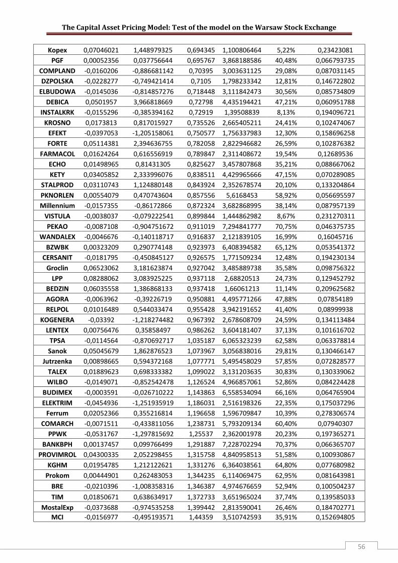
The Capital Asset Pricing Model: Test of the model on the Warsaw Stock Exchange
56
Kopex 0,07046021 1,448979325 0,694345 1,100806464 5,22% 0,23423081
PGF 0,00052356 0,037756644 0,695767 3,868188586 40,48% 0,066793735
COMPLAND -0,0160206 -0,886681142 0,70395 3,003631125 29,08% 0,087031145
DZPOLSKA -0,0228277 -0,749421414 0,7105 1,798233342 12,81% 0,146722802
ELBUDOWA -0,0145036 -0,814857276 0,718448 3,111842473 30,56% 0,085734809
DEBICA 0,0501957 3,966818669 0,72798 4,435194421 47,21% 0,060951788
INSTALKRK -0,0155296 -0,385394162 0,72919 1,39508839 8,13% 0,194096721
KROSNO 0,0173813 0,817015927 0,735526 2,665405211 24,41% 0,102474067
EFEKT -0,0397053 -1,205158061 0,750577 1,756337983 12,30% 0,158696258
FORTE 0,05114381 2,394636755 0,782058 2,822946682 26,59% 0,102876382
FARMACOL 0,01624264 0,616556919 0,789847 2,311408672 19,54% 0,12689536
ECHO 0,01498965 0,81431305 0,825627 3,457807868 35,21% 0,088667062
KETY 0,03405852 2,333996076 0,838511 4,429965666 47,15% 0,070289085
STALPROD 0,03110743 1,124880148 0,843924 2,352678574 20,10% 0,133204864
PKNORLEN 0,00554079 0,470743604 0,857556 5,6168453 58,92% 0,056695597
Millennium -0,0157355 -0,86172866 0,872324 3,682868995 38,14% 0,087957139
VISTULA -0,0038037 -0,079222541 0,899844 1,444862982 8,67% 0,231270311
PEKAO -0,0087108 -0,904751672 0,911019 7,294841777 70,75% 0,046375735
WANDALEX -0,0046676 -0,140118717 0,916837 2,121839105 16,99% 0,16045716
BZWBK 0,00323209 0,290774148 0,923973 6,408394582 65,12% 0,053541372
CERSANIT -0,0181795 -0,450845127 0,926575 1,771509234 12,48% 0,194230134
Groclin 0,06523062 3,181623874 0,927042 3,485889738 35,58% 0,098756322
LPP 0,08288062 3,083925225 0,937118 2,68820513 24,73% 0,129452792
BEDZIN 0,06035558 1,386868133 0,937418 1,66061213 11,14% 0,209625682
AGORA -0,0063962 -0,39226719 0,950881 4,495771266 47,88% 0,07854189
RELPOL 0,01016489 0,544033474 0,955428 3,942191652 41,40% 0,08999938
KOGENERA -0,03392 -1,218274482 0,967392 2,678608709 24,59% 0,134113484
LENTEX 0,00756476 0,35858497 0,986262 3,604181407 37,13% 0,101616702
TPSA -0,0114564 -0,870692717 1,035187 6,065323239 62,58% 0,063378814
Sanok 0,05045679 1,862876523 1,073967 3,056838016 29,81% 0,130466147
Jutrzenka 0,00898665 0,594372168 1,077771 5,495458029 57,85% 0,072828577
TALEX 0,01889623 0,698333382 1,099022 3,131203635 30,83% 0,130339062
WILBO -0,0149071 -0,852542478 1,126524 4,966857061 52,86% 0,084224428
BUDIMEX -0,0003591 -0,026710222 1,143863 6,558534094 66,16% 0,064765904
ELEKTRIM -0,0454936 -1,251935919 1,186031 2,516198326 22,35% 0,175037296
Ferrum 0,02052366 0,355216814 1,196658 1,596709847 10,39% 0,278306574
COMARCH -0,0071511 -0,433811056 1,238731 5,793209134 60,40% 0,07940307
PPWK -0,0531767 -1,297815692 1,25537 2,362001978 20,23% 0,197365271
BANKBPH 0,00137457 0,099766499 1,291887 7,228702294 70,37% 0,066365707
PROVIMROL 0,04300335 2,052298455 1,315758 4,840958513 51,58% 0,100930867
KGHM 0,01954785 1,212122621 1,331276 6,364038561 64,80% 0,077680982
Prokom 0,00444901 0,262483053 1,344235 6,114069475 62,95% 0,081643981
BRE -0,0210396 -1,008358316 1,346387 4,974676659 52,94% 0,100504237
TIM 0,01850671 0,638634917 1,372733 3,651965024 37,74% 0,139585033
MostalExp -0,0373688 -0,974535258 1,399442 2,813590041 26,46% 0,184702771
MCI -0,0156977 -0,495193571 1,44359 3,510742593 35,91% 0,152694805

The Capital Asset Pricing Model: Test of the model on the Warsaw Stock Exchange
57
PROSPER -0,0097629 -0,334172494 1,52825 4,032770974 42,50% 0,140724698
BORYSZEW 0,11805953 2,44632209 1,537917 2,456759907 21,53% 0,232460772
POLLENAE -0,0102319 -0,337492818 1,60607 4,084039741 43,12% 0,146034003
STALEXP -0,0254055 -0,853897985 1,624344 4,208953202 44,61% 0,143312278
ORBIS 0,00246263 0,134697806 1,636691 6,901521391 68,40% 0,088064575
MNI -0,0851334 -1,607756085 1,71336 2,494512688 22,05% 0,255059901
SWARZEDZ -0,0296098 -0,800689875 1,760399 3,669924346 37,97% 0,178128479
Interia.pl 0,00638962 0,202436448 1,766368 4,314313074 45,83% 0,152036847
WISTIL 0,09238486 1,785445987 1,772635 2,641084612 24,07% 0,249239182
IMPEXMET 0,02657942 0,774512592 1,909953 4,290648467 45,56% 0,165302422
Netia -0,0091304 -0,168531945 1,936732 2,756007853 25,66% 0,260956692
POLIMEXMS 0,00705509 0,223106946 2,003782 4,885151662 52,03% 0,152318204
GETIN 0,01846817 0,408285712 2,060134 3,51117895 35,91% 0,217882249
Kruszwica 0,05311032 1,419785422 2,254531 4,646405654 49,53% 0,180184912
KABLE -0,0023689 -0,05321078 2,26787 3,927287322 41,21% 0,214439542
Table B Portfolios’ estimated betas
Portfolio Intercept t-value Intercept Beta t-value Beta R-Square Regressions
Standard Error
1 -0,0071809 -0,45623182 0,662537 1,883688044 13,89% 0,07010307
2 0,02663747 1,383898411 -0,13477 -0,313320587 0,44% 0,085729571
3 0,02686528 2,075498819 0,770993 2,665479336 24,41% 0,057651521
4 0,02348207 1,783977304 -0,10452 -0,355337145 0,57% 0,058625814
5 0,01046269 0,939069176 0,420572 1,689228555 11,48% 0,049623535
6 -0,0133052 -1,146325573 0,852132 3,28538441 32,91% 0,051695935
7 0,01389495 1,163174599 0,431808 1,617604327 10,63% 0,053205203
8 0,00204448 0,164194534 0,552562 1,985868166 15,20% 0,055458258
9 -0,0037214 -0,385349194 0,492158 2,280559496 19,12% 0,043012883
10 0,0032004 0,379413123 0,738256 3,916594415 41,08% 0,037569364
11 0,01548905 1,938017988 0,838578 4,695373645 50,05% 0,035596622
12 0,0176784 1,641182898 0,973739 4,045297198 42,66% 0,047976415
13 -0,0109713 -1,31626553 0,366502 1,967688488 14,97% 0,037124079
14 0,00513919 0,44218482 0,607397 2,338706416 19,91% 0,051764588
15 -0,0051145 -0,245646493 0,697025 1,498121537 9,26% 0,092733632
16 0,00474533 0,482955006 0,915004 4,167322246 44,12% 0,043762445
17 0,01231443 0,737941041 1,253952 3,362652078 33,95% 0,074324968
18 -0,0035357 -0,283565333 0,664625 2,385335104 20,55% 0,055534513
19 0,00213233 0,117082388 1,226472 3,013626231 29,22% 0,08111552
20 0,02974581 1,658822757 0,386471 0,964460181 4,06% 0,079867074


![Capital Asset Pricing Theory[1]Capem](https://img.dokumen.tips/doc/110x75/577d24701a28ab4e1e9c7e2b/capital-asset-pricing-theory1capem.jpg)