Qi Zhang

The Balassa–Samuelson relationship: services, manufacturing and product quality Article (Accepted version) Refereed

Original citation: Zhang, Qi (2017) The Balassa–Samuelson relationship: services, manufacturing and product quality. Journal of International Economics, 106 . pp. 55-82. ISSN 0022-1996 DOI: 10.1016/j.jinteco.2016.10.004 Reuse of this item is permitted through licensing under the Creative Commons:

© 2017 Elsevier CC BY-NC-ND 4.0

This version available at: http://eprints.lse.ac.uk/68705/ Available in LSE Research Online: December 2016

LSE has developed LSE Research Online so that users may access research output of the School. Copyright © and Moral Rights for the papers on this site are retained by the individual authors and/or other copyright owners. You may freely distribute the URL (http://eprints.lse.ac.uk) of the LSE Research Online website.

The Balassa-Samuelson Relationship: A Micro-AnalysisI

Qi Zhang∗

London School of Economics, 32 Lincoln’s Inn Fields, London WC2A 2AE, UK

University of Oxford, Manor Road Building, Oxford OX1 3UQ, UK

Abstract

This paper shows that the specification of the Balassa-Samuelson relationship, i.e. the

positive relationship between a country’s per capita income and its national price level,

at the level of the products used in constructing national price levels is different for

‘services’ and ‘manufactures’. It further offers a new candidate explanation for the B-S

relationship in manufactures, which appeals to mismeasured quality. This explanation

yields a second, distinctive, testable prediction: controlling for per capita income, a non-

monotonic relationship should exist between a country’s income inequality and its national

price level. I show that this second prediction is consistent with empirical evidence.

Keywords: price level; income distribution; inequality; quality; Balassa-Samuelson.

JEL classifications: C43; D31; E31; F31; L15.

II thank the World Bank for granting me access to the ICP 2005 benchmark dataset. Financial supportfrom the Dorothy Hodgkin Postgraduate Awards at the London School of Economics are gratefullyacknowledged.

∗Email address: q.zhang4@lse.ac.uk

Preprint submitted to Journal of International Economics July 28, 2016

1. Introduction

The Balassa-Samuelson (B-S) relationship, first introduced in 19641, links the per

capita income level of a country to its price level, as measured by a broad price index.

Balassa and Samuelson showed that as we move towards richer countries, the measured

price level becomes higher (a.k.a. the Penn effect). This represents an apparent violation

of Purchasing Power Parity (PPP). Balassa and Samuelson proposed an explanation based

on an appeal to the presence of a service component in the national price level. Although

rich countries are relatively more productive in the traded goods sector, it is hard for them

to establish technological superiority in the labor-intensive service sector. Therefore, the

prices of services will reflect local wages, and will rise relative to the prices of traded goods

as we move from poor countries to rich countries.2

The point of departure of the present paper lies in a purely empirical analysis of the

standard dataset used in the literature. By plotting the B-S relationship for each of the

individual products used in constructing the standard national price level, it is shown that

the form of the relationship differs sharply between two groups of products. Goods in the

first group are essentially ‘pure services’ such as hairdressing. Goods in the second group

are essentially non-services, such as manufactures. It should be expected that goods in

the first group, all of whose costs are ‘local’, should not exhibit PPP. By deleting this

(large) group, I recalculate a new price level. As I am left primarily with manufactures,

the B-S relationship is not expected to hold. Yet I show that the B-S relationship remains

intact for the new price level, i.e. PPP is violated.

The central aim of this paper is to propose a new candidate explanation for the

apparent violation of PPP exhibited in the B-S relationship. Since this explanation,

unlike the traditional explanation, does not appeal to the presence of a ‘local services’

element in the national price level, it is natural to test the present model using both

the standard price level, and the modified price level that excludes the ‘services type’

products. Thus, I am not excluding the part played by services industries in driving the

B-S relationship. Rather, I am suggesting that it is not the whole story.

The candidate explanation for the apparent violation of PPP that I develop in what

follows, is based on an appeal to ‘mismeasured quality’. The idea that quality is not

fully adjusted for in conventional price indices is a long standing theme in the industrial

organization literature. The idea can be traced to the hedonic price literature (Griliches,

1961), and it has been re-explored in recent work by Pakes (2003, 2005).

1Balassa (1964) and Samuelson (1964).2This classic explanation has been heavily criticized in the literature. For example, Rogoff (1996)

showed that although there is empirical support for the model when comparisons are made between theset of ‘all poor countries’ and the set of ‘all rich countries’, this effect is not statistically significant withineither the poor countries group or the rich countries group.

2

In the context of calculating national price levels, the ICP (International Comparison

Program) has made process in controlling for quality since the introduction of structured

product descriptions (SPDs) in the 2005 round. The SPDs are used to define products,

the prices of which are collected in every country. The ideal is to have the descriptions as

precisely defined as possible, so that the prices collected based on these are comparable

across countries. However, the design of SPDs has to balance the trade-off between com-

parability and representativity, so SPDs cannot be designed precisely enough to pin down

quality. For example, due to different expenditure patterns in different countries, maybe

a precisely defined item within an expenditure category is a typical item in the consump-

tion basket of country A and hence is representative of its expenditure pattern, but the

item may not be representative in country B, even though its price might be observable in

country B. In this case, instead of using the precisely defined description to match items

between the two countries and missing the criteria of representativity, the ICP may use a

less precisely defined product description so that both countries can have representative

products to match the new description. As a result, the important characteristics that

have caused quality to exist in the disaggregated trade prices as shown in the literature,

such as producer characteristics (brand and country of origin), are generally missing in

the SPDs. Therefore, SPDs still leave large room for cross-country quality variations.

In the present setting, failure to make a full adjustment for quality levels means that,

since the average quality level of goods consumed is higher in richer countries, a spurious

correlation will appear between a country’s income level and its price level.

The model developed in this paper is a hedonic pricing model a la Rosen (1974). The

key assumption is that income elasticity of quality is positive and is higher for nontraded

goods. The motivation for this assumption is discussed below.

Within this model, we will examine the relation between a country’s income level, and

a price level that is not fully quality adjusted. Given that consumers in the countries with

higher per capita income tend to spend more on the nontraded (‘quality’) goods, this will

imply a higher measured price level in richer countries (the B-S or Penn effect). While this

first result is intuitively obvious, the model also leads to a less obvious, and distinctive,

prediction: controlling for per capita income, income inequality also has an effect on

the national price level and the effect is decreasing in per capita income. The intuition

behind the second prediction is that in the model of Rosen (1974), where consumers’

demand for quality rises in income and the price schedule of quality depends on the

distribution of income, the average price of quality in the market will be the average paid

by consumers with different income levels and hence will depend on the distribution of

income. In testing the empirical predictions of the theory in what follows, I first show

that the second prediction is consistent with empirical evidence using a price level based

on all expenditure categories. I then repeat the exercise using a modified price level which

3

excludes the ‘pure services’ categories. It is shown that even when services are excluded,

the B-S relationship survives, and the second distinctive prediction of the present theory

is consistent with the evidence.

This paper contributes to the international pricing literature by providing an alter-

native candidate explanation for the national price level, which is based on mismeasured

quality. In the existing literature, international price differentials, i.e. the violation of

PPP, have been explained by transportation and distribution costs. Crucini and Yil-

mazkuday (2014) use the retail prices of products with the same characteristics to show

that transportation and distribution costs account for over 50% of international price

dispersion at the aggregate level. Variable mark-ups have also been used to explain why

the prices of the same product vary across countries. In Simonovska (2015), the mark-up

of the same apparel or footwear rises with a country’s per capita income because per

capita income increases the consumption of each positively-consumed variety and drives

down the elasticity of substitution between these varieties. In Alessandria and Kaboski

(2011), firms charge higher mark-ups for consumers in richer countries as these consumers

value time at a premium and hence they are less willing to spend time on searching for low

prices. Hummels and Lugovskyy (2009) model the positive relationship between mark-ups

and per capita income in the ideal varieties framework, in which consumers with higher

income are willing to spend more to get closer to their ideal variety. In addition, a series

of papers in the literature have used quality to explain international price differentials.

Goldberg and Verboven (2001) and Imbs et al. (2010) show quality accounts for a large

share of the international dispersion in the prices of cars and TVs. Schott (2004) uses

product level U.S. import data to show unit values are higher for exporters with relatively

high productivity. This finding contradicts the standard trade theory and suggests the

role of quality in explaining the unit values. Crozet, Head and Mayer (2012) introduce

directly measured quality to the Melitz (2003) model of firm heterogeneity in the case of

French Champagne industry and show that quality increases firm-level prices even con-

trolling for productivity. Hallak (2006) shows that countries with high per capita income

tend to buy goods with higher qualities, which imply higher prices. Hallak and Schott

(2011), Khandelwal (2010) and Feenstra and Romalis (2014) disentangle quality from

trade unit values and show the important role of quality in explaining the cross-country

variations in unit values. In contrast, Sutton and Trefler (2016) identify the quality of

a good using a product range, i.e. the range of incomes defined by the income levels of

the poorest and richest exporters of the good, and show how quality affects the mark-up

of the good in a general equilibrium framework. Choi, Hummels and Xiang (2009) use

quality to explain the correlation between income distribution and the distribution of

import prices. Bekkers, Francois and Manchin (2012) also study the relationship between

import prices and two moments of income distribution: per capita income and income

4

inequality, but they focus on the role of hierarchic demand3 in driving the relationship.

Similarly, this paper also tries to link income distribution with prices, but instead of the

prices of imports, the emphasis is on the national price level. Fajgelbaum, Grossman and

Helpman (2011) provide a demand-based explanation for the pattern of trade in verti-

cally differentiated goods, while in this paper a demand-based explanation is given for

the role of vertically differentiated goods in the national price level. Bergstrand (1991)

distinguishes empirically the competing theories of the national price level, which include

the supply-based explanations by Balassa (1964), Samuelson (1964) and Bhagwati (1984)

and a demand-based explanation. And he finds empirical support for the demand-based

explanation.4

The rest of this paper is structured as follows. Section 2 develops the basic empirical

analysis leading to the splitting of the product set into 2 groups. Section 3 presents

the model, in which the price schedule of vertically differentiated goods is endogenously

determined by income distribution. The market equilibrium is used to examine how

income distribution affects price levels and expenditure shares. Section 4 tests the model’s

predictions at the aggregate level and at an intermediate level. Section 5 concludes.

2. The B-S Relationship at the Product Level

The point of departure of the present paper lies in a purely empirical analysis of

the standard dataset used in the literature. More specifically, the B-S relationship is

explored at the disaggregate level. The disaggregate price levels used in this paper are from

the International Comparison Program (ICP) 2005 benchmark dataset, which includes

the price levels of 129 basic headings for 146 countries.5 Basic headings are defined as

the most disaggregate price level, at which there exists matching expenditure data from

national accounts. These price levels of basic headings are just the disaggregate price

levels underlying the national price level in the Penn World Table.

One of the standard specifications characterizing the B-S relationship is

p = a+ bw, (1)

3Consumers extend their set of goods consumed as income rises.4Hassan (2015) shows that the pattern of structural change can lead to an U-shape relationship

between per capita income and national price levels. He mainly uses the supply side to explain nationalprice differentials resulting from structural change. My demand-side model and empirics complementsthe supply-side model and empirics by Hassan (2015). In particular, when I include covariates intendedto capture Hassan’s work, I find that my own key variables fall in magnitude by about one third butremain very statistically significant.

5All the results in this paper hold both when the 129 basic headings are used and when individualand collective services are excluded, as they are classified as comparison-resistant areas by the ICP dueto their imperfect price concepts.

5

where p denotes the national price level and w denotes GDP per capita.6 Here we begin

from specification (1), but we re-interpret it so as to distinguish explicitly between local

costs, represented here as labour costs7, and costs associated with internationally tradable

items. We note that PPP is expected to apply only to the second element.

Now this distinction between local and international costs has always been regarded

as (at least a contributing factor in) driving the apparent violation of PPP. But here,

we make this explicit, with a view to identifying and separating the industries, for which

costs are mainly local labour costs.

The specification in (1) can be interpreted as follows: if the market is competitive,

price is equal to marginal cost, which is a weighted average of local labour costs and

international costs,

p = MC = ϕw + (1− ϕ)ι, (2)

where ϕ is the weight and ι is the world price of the internationally tradable items, and

is constant across countries. Therefore, its reduced form yields the linear specification in

(1). And linking (2) to (1) tells us that b is equal to ϕ and a is equal to (1 − ϕ)ι. To

identify and separate those products with local labour costs as their major costs, I run

the regression implied by (1), on a product by product basis, and plot the estimates of a

and b in Figure 1.8

The open diamonds represent services (designated the ‘S-group’) and the dark squares

represent non-services (designated the ‘M-group’). Please see Appendix B.2 for the prod-

uct classification. On inspection, we have two observations. First, we notice that there

is a sharp split between pure services and non-services. For services, we expect that ϕ

is large so b is large and a is small. Indeed, b is high with a mean 0.615 and a standard

deviation 0.215 while a is statistically not very different from 0 with a mean 0.382 and

a standard deviation 0.235, suggesting that their price levels are mainly determined by

local labour costs. For non-services, ϕ is smaller. So we expect that b is smaller and a

is larger. Indeed, b is low with a mean 0.427 and a standard deviation 0.253 while a is

significantly positive with a mean 0.815 and a standard deviation 0.302. This is consistent

with the fact that their price levels rely less on local labour costs. In addition, a multi-

variate test of means can also be performed to test the hypothesis that both the means

of as and the means of bs are equalized between the S-group and the M-group, allowing

for heterogeneous covariance matrices across the two groups. The test result shows that

the hypothesis is rejected at 1% level with the F -statistic being equal to 40.13. Second,

6This specification is used in Balassa (1964).7Other local costs are rent, electricity etc., but these non-tradable items should, like labour, reflect

local conditions.8Appendix C.1 provides a modified version of Figure 1 showing the industry labels, in which we can

see more clearly the role played by tradables in the service sectors.

6

there is a large amount of heterogeneity in the estimates of a and b within non-services.

Some non-services do not exhibit the B-S relationship as their estimates of b are close to

zero. While some other non-services exhibit a strong B-S relationship with a significantly

positive estimate of b.

Figure 1: The B-S Estimation: Services vs. Non-Services

−.5

0.5

11.5

0 .5 1 1.5 2

Services Non−Services

b

a

Notes: a and b are the intercept and slope from the B-S estimation. The open di-amonds and the dark squares represent the estimates from services and non-servicesrespectively. Data from Zimbabwe are not included in the estimation due to its volatileexchange rate in 2005. The basic heading of Passenger Transport by Air is excludedfrom the figure, as its B-S relationship is downward-sloping.

Now these observations can also be analysed using alternative specifications. A second

and more popular formulation of the B-S relationship is

p = a+ b lnw, (3)

where the log of GDP per capita is used on the r.h.s. In Appendix C.2, I plot the price level

relative to the U.S. (p/pU.S.) against ln(GDP per capita/US GDP per capita) separately

for each of the ICP basic headings.9 In each plot, one data point corresponds to one

country. We expect the plots to have one of the following three patterns.

9Two basic headings, “Net Purchases Abroad” and “Balance of Exports and Imports”, are excluded,as they are not supposed to be covered by the scope of this paper.

7

1. In the extreme where ϕ = 1 so that all costs are local, we expect p = w and hence

p/pU.S. = exp(ln(GDP per capita/US GDP per capita)).

That is, we expect an exponential relationship. Panel (a) of Figure 2 displays this rela-

tionship for the case of Hospital Services.

2. In the other extreme where ϕ = 010 so that all costs are international, we expect

p = a. That is, the data should line up horizontally. Panel (b) of Figure 2 displays this

relationship for Other Cereals.

3. Intermediate cases should display a weaker exponential relationship. Panel (c) of

Figure 2 displays this relationship for Furniture.

The Figure 2 plots are representative. The more interested reader should look at all

127 plots in Appendix C.2 to convince himself or herself that these three types are very

much in evidence and appear where expected, i.e. the exponential relationship occurs for

most services and the horizontal relationship occurs for most highly-traded goods.

Now the central theme of this paper is that, even when we eliminate those products

that are primarily ‘services’, whose costs are predominantly local labour costs, the B-S

relationship remains clear, i.e. the violation of PPP is still evident. This can be seen in

Figure 3, where the B-S relationships, in its basic form (1), are plotted using the national

price level and the price level of non-services.11 Both show a positive relationship. In

addition, to check that the B-S relationship found for the price level of non-services is not

due to the aggregation method used in aggregating the prices at the product level to the

price level of non-services, I also pool the B-S scatter plots of all M -group products in

Appendix C.2 together and fit the pooled scatter plot with a non-parametric regression

curve without imposing any functional form. Figure 4 shows that the non-parametric

fitted curve also displays a B-S relationship.12 The above results motivate our search

for an alternative contributing factor, that will hold even among industries that are pure

’manufacturing’ industries (M-group products).

10Of course, ϕ can never be exactly 0 because there are always some labour costs.11The price levels of non-services are constructed using the standard Geary and Khamis (GK) method

by the PWT and the ICP Benchmark Dataset 2005.12A small number of observations above 3 are not plotted.

8

Figure 2: Three Archetypal Forms of Price-Wealth Relationships0

.2.4

.6.8

1

Pric

e o

f H

osp

ita

l S

erv

ices (

U.S

.=1

)

−5 −4 −3 −2 −1 0 1

log(GDP per capita/US GDP per capita)

(a) Hospital Services

01

23

4

Pric

e o

f O

ther C

erea

ls (

U.S

.=1

)

−5 −4 −3 −2 −1 0 1

log(GDP per capita/US GDP per capita)

(b) Other Cereals

0.5

11

.5

Pric

e o

f F

urn

itu

re (

U.S

.=1

)

−5 −4 −3 −2 −1 0 1

log(GDP per capita/US GDP per capita)

(c) Furniture

Figure 3: The B-S Relationship for Alternative Price Indexes (Based on Equation (1))

AGO

ALB

ARG

ARM

AUSAUT

AZEBDI

BEL

BENBFA

BGD

BGR

BHR

BIH

BLRBOL

BRA

BRN

BTN

BWACAF

CAN

CHE

CHL

CHN

CIV

CMR

COG

COL

COM

CPV

CYP

CZE

DJI

DNK

ECU

EGY

ESP

EST

ETH

FIN

FJI

FRA

GAB

GBR

GEO

GER

GHA

GINGMB

GNB

GNQGRC

HKG

HRVHUN

IDN

IND

IRL

IRN

IRQ

ISL

ISR

ITA

JOR

JPN

KAZKEN

KGZ

KHM

KORKWT

LAO

LBN

LBR

LKA

LSO LTU

LUX

LVA

MACMAR

MDA

MDG

MDV

MEX

MKD

MLI

MLT

MNE

MNG

MOZ

MRT

MUS

MWI

MYS

NAM

NERNGA

NLD

NOR

NPL

NZL

OMN

PAK

PER

PHL

POL

PRT

PRY

QAT

ROM

RUS

RWA

SAU

SDN

SEN

SGP

SLESRB

STPSVK

SVN

SWE

SWZ

SYR

TCDTGO

THA

TJK

TUN

TUR

TWN

TZAUGA

UKR

URY

USA

VEN

VNM

YEM

ZAF

ZARZMB

0.5

11.

5N

atio

nal

Pri

ce L

evel

(U

.S.=

1)

0 .5 1 1.5 2GDP per capita (U.S.=1)

(a) The B-S Relationship Using the National PriceLevel

AGO

ALB

ARGARM

AUS

AUT

AZEBDI

BEL

BEN

BFA

BGD

BGR

BHR

BIH

BLR

BOL

BRA

BRN

BTN

BWA

CAF

CAN

CHE

CHL

CHN

CIV

CMR

COG

COL

COMCPV

CYP

CZE

DJI

DNK

ECU

EGY

ESP

EST

ETH

FIN

FJI

FRA

GAB

GBR

GEO

GER

GHA

GINGMB

GNB

GNQ

GRC

HKG

HRVHUN

IDN

IND

IRL

IRN

IRQ

ISL

ISR

ITA

JOR

JPN

KAZKEN

KGZ

KHM

KOR

KWT

LAO

LBN

LBR

LKA

LSO LTU

LUX

LVAMAC

MAR

MDAMDG

MDVMEX

MKD

MLI

MLT

MNE

MNG

MOZ

MRT

MUS

MWI

MYS

NAM

NER

NGA

NLD

NOR

NPL

NZL

OMN

PAK

PER

PHL

POL

PRT

PRY

QAT

ROM

RUS

RWA

SAU

SDNSEN

SGP

SLE

SRB

STP

SVK

SVN

SWE

SWZ

SYR

TCD

TGO

THA

TJK

TUN

TUR

TWN

TZA

UGAUKR

URY

USA

VEN

VNMYEM

ZAF

ZAR

ZMB

0.5

11

.5

Pric

e L

ev

el

of

M−

gro

up

Pro

du

cts

(U

.S.=

1)

0 .5 1 1.5 2

GDP per capita (U.S.=1)

(b) The B-S Relationship Using the Modified PriceLevel that Excludes ‘Services Type’ Products

In the next section, I develop an alternative candidate explanation for the B-S re-

9

Figure 4: The Pooled Scatter Plots of all M -group Products

01

23

Pric

e o

f M

−g

ro

up

Pro

du

cts

(U

.S.=

1)

−5 −4 −3 −2 −1 0 1

log(GDP per capita/US GDP per capita)

Notes: The non-parametric curve with 95% confidence intervals is obtainedusing local-mean smoothing with a bandwidth of 1.5.

lationship, appropriate to the M -group products, based on an appeal to mismeasured

quality.

3. A ‘Mismeasured Quality’ Interpretation

This section begins with the basic intuition behind the distinctive prediction of the

model, i.e. the non-monotonic relationship between income inequality and the national

price level. Then it describes the consumer’s problem, in which an empirically motivated

key assumption is reflected, the producer’s problem and the market equilibrium. Finally,

an analytical solution of the equilibrium is used to derive propositions regarding how in-

come distribution affects expenditure shares and price levels at disaggregate and aggregate

levels.

3.1. The Basic Intuition

The model developed in this paper is a hedonic pricing model a la Rosen (1974),

in which consumers and firms choose their optimal positions along an equilibrium price

schedule p(z), where z is a vector of characteristics of the good in question. As firms take

the equilibrium price schedule as given in their profit maximization problem, the price of

any quality good is equal to its marginal cost. Hence the mark-up is fixed to be 1 and

does not play any role in this paper.

10

The focus of the analysis lies in establishing a relationship between a country’s level

of income, and – more importantly – the form of income distribution in the country, and

the pattern of demand for both ‘quality’ goods and ‘homogeneous’ goods.

The novel prediction of the model is that controlling for per capita income, income

inequality also affects the national price level. The basic intuition of this is: a higher

income inequality implies that a consumer has to pay more to switch from a low quality

good to a high quality good as the prices of high quality goods are raised by the newly

created rich people. As a result, consumers will lower the share of income spent on

quality goods and increase the share on homogeneous goods. A simple illustration of this

mechanism is: suppose a country’s per capita income is µ∗ and its income distribution is

made up of three income groups with equal population. The top income group consumes

a top quality good, the middle income group consumes a middle quality good and the

bottom income group consumes a bottom quality good. Given the same Cobb-Douglas

utility function, everyone spends a same fraction θ of his/her income on quality goods.

As quality cannot be fully controlled for, the implied price level of quality goods will

depend on the average expenditure on it, which is equal to µ∗θ. Now consider a mean-

preserving spread of income distribution, which means that there are now less people in

the middle income group and more people in the top and bottom groups. This income

redistribution will increase the quantity demanded of the top and bottom quality goods.

As the marginal cost function of the quality good is increasing in the number of units

produced, the increased demand will increase the prices of the top and bottom quality

goods, resulting in a more convex price function. With a more convex price function of

quality goods and the unit elasticity of substitution in the Cobb-Douglas utility function,

all consumers will spend a lower fraction θ′ (< θ) of income on quality goods. As a result,

its measured price level will be lower, as the average expenditure on quality goods, is

now reduced to µ∗θ′. This is the mechanism through which income inequality affects the

national price level in the present model.

3.2. The Model I: The Consumer’s Problem

On the consumer’s side, in every country there is a unit mass of consumers indexed by

income level c. The income distribution is assumed (conventionally) to follow the Pareto

distribution characterized by two parameters kc and cm, where cm is the lower bound of

income level c and kc is the shape parameter. Hence the probability density function of

income is

f(c) = kcckcmc−(kc+1), kc > 1, c ∈ [cm,∞).

Quality enters the utility function in a way similar to Flam and Helpman (1987), who

introduce quality to their model of North-South trade. That is, consumer preferences are

represented by a utility function v(x, z), where x is the quantity of a homogeneous good,

11

denoted by X, and z is the quality of a vertically differentiated good denoted by Z. In

this paper, I further assume that the homogeneous good is tradable and the vertically

differentiated good is nontradable and hence locally priced. Therefore, a consumer with

income c chooses the quantity of the homogeneous good and the quality level of the

vertically differentiated good to solve the following utility maximization problem:

maxx,z

v(x, z)

s.t. c = x+ p(z). (4)

where p(z) is the nonlinear hedonic price function of the vertically differentiated good,

which is set locally, and the price of the homogeneous good is one.

The utility function assumed above reflects two key assumptions in the consumer’s

problem. The first is that income elasticity of quality varies across goods and is high

for many goods. To reflect this, I include both homogeneous goods (with zero income

elasticity of quality) and vertically differentiated goods (with positive income elasticity of

quality) in the model. I motivate this assumption by reference to Bils and Klenow (2001),

which provide empirical support for this assumption. They estimate income elasticities

of quality and income elasticities of quantity for 66 durable goods and find that income

elasticity of quality is positive and non-negligible.13 For many goods in their sample,

income elasticity of quality is higher relative to that of quantity. For example, for goods

such as window coverings, curtains and drapes, the quality consumed rises sharply relative

to the quantity as household income rises. In contrast, for goods such as clothing and

footwear, the quantity consumed tends to increase by more than the quality as household

income rises. The second assumption is that income elasticity of quality is higher for

nontraded good. To reflect this, the homogeneous good is assumed to be tradable and the

vertically differentiated good is assumed to be nontradable in the model. This assumption

can be supported by a significant negative relationship between tradability and income

elasticity of quality for the goods studied in Bils and Klenow (2001). The details are

shown in Appendix C.4. In addition to tradable homogeneous goods and non-traded

vertically differentiated goods, I abstract from other types of goods for the following

reasons. First, I let traded goods be homogeneous for analytical simplicity. Second,

homogeneous nontradables, which are the focus of the B-S model, are not included in

the present model. Furthermore, the significant negative relationship between tradability

and income elasticity of quality also suggests that we can abstract from other goods and

focus on the traded homogeneous goods and the nontraded vertically differentiated goods

13Appendix C.3 provides additional empirical evidence on the relative importance of income elasticitiesof quality and quantity for food, houses, clothes and vehicles.

12

in the model without loss of generality.

In what follows I assume the utility function v(x, z) is a standard Cobb-Douglas utility

function, i.e. v(x, z) = xαzβ, α+β = 1. Given this, the Lagrangian for the problem in (4)

is given by

L = xαzβ + λ[c− x− p(z)].

First-order necessary conditions imply that

vzvx

= p′(z) and henceβ

α

x

z= p′(z).

Combining it with the budget constraint x = c− p(z), we have

c = (α/β)zp′(z) + p(z), (5)

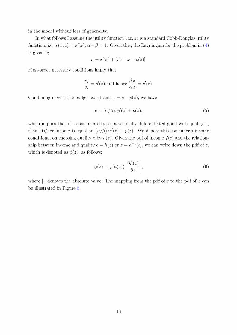
which implies that if a consumer chooses a vertically differentiated good with quality z,

then his/her income is equal to (α/β)zp′(z) + p(z). We denote this consumer’s income

conditional on choosing quality z by h(z). Given the pdf of income f(c) and the relation-

ship between income and quality c = h(z) or z = h−1(c), we can write down the pdf of z,

which is denoted as φ(z), as follows:

φ(z) = f(h(z))

∣∣∣∣∂h(z)

∂z

∣∣∣∣ , (6)

where |·| denotes the absolute value. The mapping from the pdf of c to the pdf of z can

be illustrated in Figure 5.

13

Figure 5: Mapping From Income Distribution to Distribution of Quality Demanded

Incomec

f(c)

cm c∗

Qualityz

Qd(z)

zm z∗

c∗ = (α/β)z∗p′(z∗) + p(z∗) = h(z∗)

Qd(z) = φ(z) = f(h(z))|∂h(z)

∂z|

Notes: Given the exogenous income distribution f(c) and the relationship between in-come and quality derived from the utility maximization problem c = h(z), the distri-bution of quality demanded Qd(z) can be obtained. c∗ = (α/β)z∗p′(z∗) + p(z∗) is therelationship between an individual’s income c∗ and the quality he/she chooses to consumez∗.

Substituting for h(z) and f(·) in (6) yields

φ(z) = f(α

βzp′(z) + p(z))

∣∣∣∣∣∂[αβzp′(z) + p(z)]

∂z

∣∣∣∣∣= kcc

kcm [α

βzp′(z) + p(z)]−(kc+1)

∣∣∣∣αβ [p′(z) + zp′′(z)] + p′(z)

∣∣∣∣ .If we denote the quantity demanded for the good with quality z by Qd(z), then the

market demand in a small interval dz near quality z is given by the product of the pdf of

quality around z, φ(z), and the length of the interval:

Qd(z)dz = kcckcm [α

βzp′(z) + p(z)]−(kc+1)

∣∣∣∣αβ [p′(z) + zp′′(z)] + p′(z)

∣∣∣∣ dz. (7)

14

3.3. The Model II: The Producer’s Problem

Although different countries have different income distributions, the supply side is the

same for all countries. In every country, there is a unit mass of firms producing vertically

differentiated goods indexed by product quality z. The distribution of the firms is assumed

to be the Pareto distribution characterized by two parameters kz and zm, where zm is the

lower bound of product quality z and kz is the shape parameter.14 Therefore, the pdf of

z takes the following form:

g(z) = kzzkzm z−(kz+1), kz > 1, z ∈ [zm,∞). (8)

As in Rosen (1974), producers in all countries are assumed to have the same cost

function ∆(M, z) = AzMτzγ, τ > 1, γ > 1, where Az is the productivity parameter and

M denotes the number of units of the product with quality z that the firm produces. It

is assumed that τ > 1 and γ > 1, which ensure that total cost is a convex function in M

and z.

The producers are price takers. Furthermore, it is assumed that the producers can

vary M but not z. (i.e. a producer’s quality is a given parameter in the short run).

Therefore, the producer’s problem is to maximize profit by choosing its output level M :

maxM

Mp(z)−∆(M, z).

The first-order conditions imply that

p(z) =∂∆

∂M= AzτM

τ−1zγ.

Thus,

M(z) = (p(z)

Azτzγ)1/(τ−1). (9)

If we denote the firms’ output of z as Qs(z), then the market supply in a small interval

dz near quality z is given by the product of the pdf of the firms around z, the quantity

14The reasons for using the Pareto distribution, a power law probability distribution, are not onlythat a closed form solution can be obtained but also that this assumption is consistent with empiricalevidence. Gaffeo, Gallegati and Palestrini (2003) analyze the average size distribution of a pool of the G7group firms over the period 1987-2000. They find that the empirical distributions are all consistent withthe power law. Luttmer (2007) also shows that the firm size distribution follows the Pareto distributionover much of its range using the U.S. data in 2002. In the model of this paper, the quality of a firm is apower transformation of the size of the firm, so it is reasonable to assume quality also follows the Paretodistribution as the Pareto distribution is close under power transformation.

15

supplied by each firm producing quality z and the length of the interval:

Qs(z)dz = g(z)M(z)dz

= kzzkzm z−(kz+1)(

p(z)

Azτzγ)1/(τ−1)dz. (10)

Figure 6 shows the mapping from the distribution of firms by quality to the distribution

of quality supplied.

Figure 6: Mapping From Firm Distribution by Quality to Distribution of Quality Supplied

Qualityz

g(z)

zm z0

g(z0)dz

Qualityz

Qs(z)

zm z0

g(z0)M(z0)dz

Qs(z) = g(z)[p(z)

Azτzγ]1/(τ−1)

Notes: Given the initial distribution of firms g(z) in (8) and the output of each firm M(z)in (9), the distribution of quality supplied Qs(z) can be derived, as illustrated, and takesthe form of (10). g(z0)dz is the number of firms that produce z0 and g(z0)M(z0)dz istotal quantity of z0 supplied.

3.4. Market Equilibrium

An equilibrium is defined as a triple {z(c),M(z), p(z)}, where z(c) is the policy func-

tion for consumers, M(z) is the policy function for producers, and p(z) is the price sched-

ule, such that:

1. z(c) solves the consumer’s utility maximization problem taking p(z) as given.

2. M(z) solves the producer’s profit maximization problem taking p(z) as given.

16

3. Market clearing: demand is equal to supply for Z goods, i.e., Qs(z) = Qd(z) for all

z.

3.5. An Analytical Solution

In equilibrium, we must have the market clearing condition Qs(z)dz = Qd(z)dz. It can

be used to solve for a solution15 to the equilibrium price function, in which the parameters

of the price function can be expressed as functions of the income distribution parameters

kc and cm. This is summarized in Lemma 1.

Lemma 1. The price function

p(z) = b(kc, cm)zd(kc), z ∈ [zm,∞)

where

b(kc, cm) =

kcc

kcm

[αβkz+γ/(τ−1)kc+1/(τ−1) + 1

]−kc kz+γ/(τ−1)kc+1/(τ−1)

kzzkzm ( 1Azτ

)1/(τ−1)

(τ−1)/[kc(τ−1)+1]

, (11)

d(kc) =kz + γ/(τ − 1)

kc + 1/(τ − 1), d′(kc) < 0 (12)

and zm is such that

cm =α

βzmp

′(zm) + p(zm).

satisfies the market clearing condition Qs(z) = Qd(z).

Proof : See Appendix A.1.

3.6. Income Distribution and Expenditure Shares

It can be shown that the expenditure share on Z goods, i.e. the price paid for Z good

divided by income p(z)/c, crucially depends on the convexity of the price function d as

p(z)

c=

p(z)αβzp′(z) + p(z)

=bzd

αβbdzd + bzd

=1

αβd+ 1

. (13)

The first equality follows from the first order condition (5) and the second equality follows

from the form of price function in Lemma 1. Furthermore, as the convexity d crucially

depends on income distribution parameter kc from (12), we can now derive the relationship

between income distribution and expenditure shares. As the Gini coefficient and per

capita income of the Pareto distribution can be expressed as analytical functions of the

15I adopt the standard method of undetermined coefficients to find a particular solution of the formp(z) = bzd, with b, d > 0, which is then substituted into the market clearing condition to solve for thevalues of the parameters b and d (Zwillinger (1997), P415).

17

distribution parameters, viz. Gini = 1/(2kc − 1) and µ = cmkc/(kc − 1), we can also

think of the Pareto distribution as governed by two independent parameters Gini and

µ. Therefore, from (12) and (13) we can derive how the Gini coefficient and per capita

income affect the convexity of the price function d and hence the expenditure shares. The

results are summarized in Proposition 1.

Proposition 1. (Income Distribution and Expenditure Shares) Income inequality has apositive impact on the expenditure share of X goods and a negative impact on the expen-diture share of Z goods. Per capita income has no impact on expenditure shares.

Proof : See Appendix A.2.

The intuition behind the first prediction of Proposition 1 is that an increase in the

Gini coefficient implies an increase in d and hence a more convex price function. As

a result, the marginal utility derived from Z goods becomes more expensive. Due to

the high substitutability between X goods and Z goods, consumers will spend a smaller

fraction of their expenditure on Z goods and more on X goods. This mechanism of

how income inequality affects expenditure shares is crucial in determining how income

inequality influences the price levels, which will be provided in the next subsection. The

second prediction is a direct implication of the Cobb-Douglas utility function. The Cobb-

Douglas utility function is used for analytical simplicity, as it can yield a closed form

solution. However, with more general utility functions, such as the CES utility function,

the results in this paper will still hold as long as the elasticity of substitution between the

two goods is high enough.

3.7. Income Distribution and Price Levels

We now explore the implications of the model for disaggregate and aggregate price

levels and how the implications are affected by the extent to which quality is adjusted.

The two polar cases are:

1. Perfect quality measurement.

2. Quality is not fully adjusted using hedonics such as in Pakes (2003).

First, in the case of perfect quality measurement, quality can be fully observed, so

in terms of the setting of the model we will be able to use the hedonic regression to

estimate the parameters in the price function p(z). Then the price schedule p(z) from

each country can be used to compare the price level of Z goods across countries. One

way of constructing the price level of Z goods while minimizing the impact of quality

in it is to use pj(z0) = bjzdj0 as the price level of Z goods in country j, where bj and

dj are the estimated parameters in country j and z0 is a constant level of quality across

countries. As a result, the price levels of Z goods in country i and country j are given by

pi(z0) = bizdi0 and pj(z0) = bjz

dj0 . The difference between the two price levels are only due

to the different bs and ds but not due to different qualities. Although in this case quality

18

can be fully controlled for, (11) implies that there still exists the B-S relationship. To

see this, suppose we keep a country’s Gini coefficient constant and increase its per capita

income, this implies a constant kc but a higher cm in the Pareto distribution. From (12)

and (11), d will stay constant but b will go up, resulting in an upward shift of the price

schedule p(z). Hence, for any quality goods, the price will be higher than before. This is

because a higher level of per capita income will increase the demand for the higher quality

Z goods and the resulting higher output will increase their prices as the marginal cost

is increasing in output. The magnitude of this B-S relationship can be measured by the

elasticity of the price level p(z0) with respect to per capita income µ, which is equal to

kc(τ − 1)/[kc(τ − 1) + 1] from (11).

However, the above procedures face a prominent practical issue. The issue is that

quality cannot be perfectly controlled for Z goods. Pakes (2003) shows how to use hedonics

to adjust quality biases in the price indexes of quality goods due to the introduction of

new goods in the case of PC, as the traditional price indexes used by the Bureau of Labor

Statistics (BLS) do not make any adjustment for the differences in the utility per dollar

between the new good and the good(s) it replaces. However, the adjustment procedures

require a complete dataset on the characteristics of the goods, which is impossible in the

case of cross-country price comparison. Without the level of quality being observed and

the price schedule p(z) being estimated, the common practice of constructing the price

index of Z goods is to use some partial quality adjustment methods such as matching

precisely defined items and calculate the average of the observed prices of all Z goods.

As a result, the price index of Z goods will generally depend on the average expenditure

on Z goods and these two will become equal when there is no quality adjustment at all.

The consequence of the practice is that the resulting price level is less informative than

in the case of perfect quality measurement as a higher price level could be either due to

higher values of b and d in the price function or simply due to the fact that the prices

of higher quality goods have been observed. This will lead to a higher B-S effect, i.e. a

higher elasticity of the price level with respect to per capita income.

To see this, suppose there is no quality adjustment and we simply use the average

expenditure on Z goods, which is equal to16

p = µβ

α kz+γ/(τ−1)(1/Gini+1)/2+1/(τ−1) + β

, (14)

as its price level, then the elasticity of the price level with respect to per capita income

µ is equal to 1, compared with a elasticity of kc(τ − 1)/[kc(τ − 1) + 1] in the previous

case of full quality adjustment. Motivated by the different elasticities in the two polar

16Please see Appendix A.3 for the derivation.

19

cases, I assume the general form of the relationship between the measured price level

with partial quality adjustment p∗ and the average expenditure p is p∗ = pη, where

kc(τ − 1)/[kc(τ − 1) + 1] < η < 1. Here, η is used to govern the extent to which quality

is adjusted. η − kc(τ − 1)/[kc(τ − 1) + 1] is the part of the elasticity of the price level

with respect to per capita income that is due to imperfect quality adjustment. Given this

assumption, we can derive how income distribution affects the measured price levels with

partial quality adjustment at the disaggregate and aggregate levels and the role played

by η in it.

First, the effects of per capita income and income inequality on the price level of Z

goods are derived. The results are summarized in Proposition 2.

Proposition 2. (Income Distribution and the Disaggregate Price Level) Per capita in-come has a positive impact on the price level of Z goods (∂p∗/∂µ > 0), whereas incomeinequality has a negative impact (∂p∗/∂Gini < 0). Moreover, the effect of income inequal-ity on the price level of Z goods is decreasing in per capita income (∂2p∗/∂Gini∂µ < 0).

Proof : See Appendix A.4.

Proposition 2 first shows that the B-S effect exists for the price level of Z goods.

Moreover, from the proof, it is easy to see that the effect would disappear if η could go

to zero. The dependence of the B-S effect on η implies that this effect can be attributed

to two sources. One source is imperfect quality adjustment, which is governed by η −kc(τ − 1)/[kc(τ − 1) + 1]. The other source is increasing marginal cost, which is governed

by kc(τ − 1)/[kc(τ − 1) + 1]. The magnitude of kc(τ − 1)/[kc(τ − 1) + 1] crucially depends

on the cost function parameters τ and could be arbitrarily small as τ approaches 1 from

above, while the magnitude of imperfect quality adjustment is exogenous and is likely

to be large given the difficulty of controlling for quality in reality. Therefore, imperfect

quality adjustment plays an important role in the B-S relationship of Z goods.

Proposition 2 also shows that keeping per capita income constant, income inequality

can also affect the price level of Z goods. This is because the price level of Z goods depends

on the average expenditure on Z goods, which is the product of the expenditure share and

per capita income. As income inequality has a negative impact on the expenditure share of

Z goods as shown in Proposition 1, income inequality can affect the price level of Z goods

through the expenditure share and the effect is decreasing in per capita income. Moreover,

from the proof the impact of income inequality increases as η goes up, suggesting the

impact of income inequality decreases with the degree of quality adjustment. As the price

level of X goods is constant across countries, the above effects of income distribution on

the price level of Z goods will play important roles in the relationship between income

distribution and the national price level.

To investigate the implications of income distribution for the national price level, we

need to construct an aggregate price index for both X goods and Z goods. Here for

20

analytical simplicity, I use the bilateral Fisher index, which is the geometric mean of the

Laspeyres index and the Paasche index, as a proxy for the national price level. This is

because the methods of computing the national price level in practice, such as the Eltero-

Koves-Szulc (EKS) and Geary and Khamis (GK) methods, are not analytically tractable,

but Deaton and Heston (2010) has shown that the national price level in the Penn World

Table can be well approximated by the geometric mean of the Laspeyres index and the

Paasche index. The Laspeyres and Paasche indices are both weighted averages of the price

ratios of disaggregate price levels relative to the base country, the U.S. In the Laspeyres

index, the weights are given by the expenditure shares of the base country, while in the

Paasche index the weights are given by the expenditure shares of the country in question.

In the model of this paper, there are two types of goods: X goods and Z goods, so the

Paasche index PP , the Laspeyres index PL and the bilateral Fisher index PF are defined

as follows:

PP ≡(

1

1sharex +

p∗0p∗sharez

)−1=

(αd

αd+ β+p∗0p∗

β

αd+ β

)−1,

PL ≡1

1sharex,0 +

p∗

p∗0sharez,0 =

αd0αd0 + β

+p∗

p∗0

β

αd0 + β,

PF ≡√PPPL,

where 0 is used in the subscript to denote variables from the base country, i.e. U.S. p∗0 and

p∗ are the measured price levels of Z goods in the base country and the country in question.

Given the definition of the national price level, in Proposition 3 the results regarding how

income distribution affects the national price level are shown. More specifically, to make

the results comparable with the empirical tests in Section 4, the results regarding how

the log of per capita income and the Gini coefficient affect the log of the national price

level are shown.

Proposition 3. (Income Distribution and the National Price Level) The impact of percapita income on the national price level is positive: the elasticity of the national pricelevel with respect to per capita income is positive (ePF ,µ ≡ (∂PF/∂µ)µ/PF > 0). Theimpact of income inequality on the national price level is decreasing in per capita income:the semi-elasticity of the national price level with respect to income inequality is decreasingin per capita income (∂ePF ,Gini/∂µ < 0, where ePF ,Gini ≡ (∂PF/∂Gini)/PF ).

Proof : See Appendix A.5.

Empirically, this proposition suggests that in a cross-sectional setting, one should

regress the national price level on per capita income and the interaction of per capita

income and the Gini coefficient, where we expect the coefficient on per capita income to

be positive and the coefficient on the interaction term to be negative.

21

Given the constant price level of X goods, we can use the intuition derived from

Proposition 2 regarding the effects of income distribution on the price level of Z goods

to understand the effects of income distribution on the national price level. First, given

the positive impact of per capita income on the price level of Z goods, per capita income

will have a positive impact on the national price level, which is a weighted average of the

price levels of X goods and Z goods. However, the elasticity of the national price level

with respect to per capita income is less than that of the price level of Z goods as the

elasticity of the price level of X goods with respect to per capita income is 0.

Second, although income inequality has a negative impact on the price level and the

expenditure share of Z goods, it is not necessary that income inequality has a negative

impact on the national price level. This is because the impact of income inequality on the

national price level also depends on the relative magnitudes of the price ratio of X goods

and Z goods relative to the base country as shown in the definition of the national price

level.

Finally, as income inequality has a negative impact on the expenditure share of Z

goods and the price level of Z goods and the national price level both depend on the

average expenditure on Z goods, which is the product of the expenditure share on Z

goods and per capita income, the impact of income inequality on the price level of Z

goods and the national price level will be decreasing in per capita income.

To summarize, the model developed in this section predicts the B-S relationship, i.e.

the positive relationship between per capita income and the national price level, and

a non-monotonic relationship between income inequality and the national price level.

And from the proof the magnitudes of all these impacts depends positively on η, which is

negatively related to the extent to which quality is adjusted. Therefore the model provides

a mismeasured quality explanation of the relationship between the national price level and

income distribution.

Compared with this explanation, the other explanations of the B-S effect cited in

the introduction generally have a demand side based on the representative agent frame-

work, i.e. all the consumers in a country are represented by a single consumer. As a

result, income distribution is degenerate and no relationship between income inequal-

ity and prices can be implied from these models. However, there are three exceptions,

in which a non-degenerate income distribution is specified. They are Bekkers, Francois

and Manchin (2012), Choi, Hummels and Xiang (2009) and Fajgelbaum, Grossman and

Helpman (2011). Due to the presence of income distribution in these models, they can

generate implications for the relationship between income distribution and prices. In

Bekkers, Francois and Manchin (2012), they use trade data and find a positive relation-

ship between per capita income of importing countries and import prices and a negative

relationship between their income inequalities and import prices. They propose three

22

models to explain these empirical findings, including a quality expansion model, an ideal

variety model and a hierarchic demand model. All three models can generate a positive

relationship between per capita income and import prices. But only the hierarchic de-

mand model can generate a negative relationship between income inequality and import

prices, while the other two models generate the opposite. As their paper is mainly about

import prices, and my paper is mainly about national price levels, there is no direct com-

parison between the two papers. However, Proposition 2 of my paper does predict three

relationships between income distribution and the price of Z goods, i.e. the vertically

differentiated goods in my model, which are a positive relationship between per capita in-

come and the price of Z goods, a negative relationship between income inequality and the

price of Z goods and the impact of income inequality on the price of Z goods is decreas-

ing in per capita income. If we view import prices in their paper as prices of vertically

differentiated goods in my model, then their preferred explanation, i.e. the hierarchic

demand model can generate the first two relationships in Proposition 2, i.e. the positive

relationship between per capita income and import prices, and the negative relationship

between income inequality and import prices but not the third relationship, i.e. the im-

pact of income inequality on the price of Z goods is decreasing in per capita income.

The third relationship is crucial in generating the nonlinear relationship between income

inequality and national price levels in my paper, which is shown to be consistent with

the data. Choi, Hummels and Xiang (2009) theoretically derive the general relationship

between income distribution and distribution of import prices. However, no conclusive

relationship between income inequality and price levels can be implied from their results,

as if we want to do so, we have to make assumptions about the functional form of income

distribution and how to aggregate prices into price levels. As a result, the relationship be-

tween income inequality and price levels will depend on the assumption made and will be

in general ambiguous. Fajgelbaum, Grossman and Helpman (2011) develop a framework

to study patterns of trade in horizontally and vertically differentiated products. In their

model, a non-degenerate income distribution is specified and goods with higher quality

imply higher prices. However, their model’s prediction regarding how income inequal-

ity affects the average quality demanded in the economy is ambiguous. As a result, no

conclusive relationship between income inequality and prices can be predicted by their

model. Therefore, existing explanations of the B-S effect cannot be easily extended or

modified to account for the empirical relationship between income distribution and the

national price level found in my paper, but my paper provides a relatively simple model

to account for that.

23

4. Empirical Evidence

This section tests the model’s predictions at two levels: the aggregate level and an

intermediate level. The aggregate price levels are from the Penn World Table (PWT),

which are commonly used to compare price levels across countries or compute real GDPs

in constant internationally comparable dollars. To construct these price levels, the Inter-

national Comparison Program (ICP) at the World Bank collects the prices of a detailed

list of goods and services in selected countries and years. The countries from which the

ICP has collected data on prices in a given year are called benchmark countries and the

given year is called a benchmark year. The collected detailed prices are first aggregated

into the price levels of basic headings. Basic headings are the most disaggregate level

at which there exist matching expenditure data from national accounts. The PWT then

aggregates the price levels at the basic heading level in the benchmark dataset into a

national price level using expenditure data from national accounts as weights. For non-

benchmark countries and years, the price levels are inferred from fitted values of price

regression run on benchmark dataset. In this paper, I concentrate on the benchmark

year 2005, for which national price levels are available in the PWT and disaggregate price

levels are available in the ICP Benchmark Dataset 2005.

4.1. Testing the Model: the Standard Index

In addition to the B-S relationship, i.e. a positive relationship between per capita

income and the national price level, the model developed in Section 3 also predicts that

income inequality can affect the national price level and the impact is decreasing in per

capita income. In this subsection, these model’s predictions are tested using data at the

aggregate level.

To show that not only per capita income but also income inequality is important in

determining the national price level, I extend the regression in Rogoff (1996) by introduc-

ing the Gini coefficient as an additional explanatory variable to investigate if it can help

to explain national price differentials.

24

Figure 7: Price Level versus GDP per capita in 2005 (U.S.=1)

AFG

AGO

ALB

ARE

ARG

ARM

ATG

AUSAUT

AZEBDI

BEL

BENBFA

BGD

BGR

BHR

BHS

BIH

BLR

BLZ

BMU

BOL

BRA

BRBBRN

BTN

BWACAF

CAN

CH2

CHE

CHL

CHN

CIV

CMR

COG

COL

COM

CPV

CRICUB

CYP

CZE

DJI

DMA

DNK

DOM

DZAECU

EGYERI

ESP

EST

ETH

FIN

FJI

FRA

FSMGAB

GBR

GEO

GER

GHA

GINGMB

GNB

GNQGRC

GRDGTM

GUY

HKG

HND

HRV

HTI

HUN

IDN

IND

IRL

IRN

IRQ

ISL

ISR

ITA

JAM

JOR

JPN

KAZKEN

KGZ

KHMKIR

KNA

KORKWT

LAO

LBN

LBR

LBYLCA

LKA

LSO LTU

LUX

LVA

MACMAR

MDA

MDG

MDV

MEX

MHL

MKD

MLI

MLT

MNE

MNG

MOZ

MRT

MUS

MWI

MYS

NAM

NERNGA

NIC

NLD

NOR

NPL

NZL

OMN

PAK

PAN

PER

PHL

PLW

PNG

POL

PRI

PRT

PRY

QAT

ROM

RUS

RWA

SAU

SDN

SEN

SGP

SLB

SLESLV

SOM

SRB

STP

SUR

SVK

SVN

SWE

SWZ

SYC

SYR

TCDTGO

THA

TJK

TKMTLSTON

TTOTUN

TUR

TWN

TZAUGA

UKR

URY

USA

UZB

VCT

VEN

VNMVUTWSM

YEM

ZAF

ZARZMB

0.5

11.

5N

atio

nal

Pri

ce L

evel

(U

.S.=

1)

0 .5 1 1.5 2GDP per capita (U.S.=1)

Notes: The fitted line is obtained by regressing the logarithm of National PriceLevel on the logarithm of GDP per capita.

Table 1: Income Distribution and the National Price Level

Relative Price Level log(Pj/PU.S.)

Independent Variable (1) (2) (3) (4)

log(Yj/YU.S.) 0.186∗∗∗ 0.719∗∗∗ 0.919∗∗∗ 0.709∗∗∗

(0.0171) (0.0854) (0.117) (0.0857)

Gini -2.623∗∗∗ -2.651∗∗∗ -2.594∗∗∗

(0.510) (0.606) (0.510)

Gini× log(Yj/YU.S.) -1.359∗∗∗ -1.649∗∗∗ -1.335∗∗∗

(0.218) (0.307) (0.218)

VAT -0.00108

(0.00405)

Population -0.000182

(0.000157)

Constant -0.232∗∗∗ 0.763∗∗∗ 0.905∗∗∗ 0.759∗∗∗

(0.0409) (0.192) (0.241) (0.192)

Observations 189 153 90 153

R2 0.388 0.541 0.717 0.545

Notes: Standard errors are in parentheses. ∗∗∗, ∗∗ and ∗ indicate signifi-cantly different from zero at the 1%, 5% and 10% level respectively.

25

First, to show that the problem with the Balassa-Samuelson relationship pointed out

in Rogoff (1996) still persists in 2005, Figure 3 in Rogoff (1996) is replicated in Figure

7 using the 2005 data in PWT 7.1. I exclude Zimbabwe from the figure due to its very

volatile exchange rate in 2005. As shown in Figure 3 of Rogoff (1996), Figure 7 still shows

that the B-S relationship performs well for the whole sample but does not perform well

either within poor countries or within rich countries, suggesting the need to find other

important explanatory variables of the national price level.

Guided by the importance of income inequality in the model, I replicate the regressions

in Rogoff (1996) but adding the Gini coefficient as an extra explanatory variable, as shown

in Table 1. Pj/PU.S. is the price level of country j relative to the United States, and

Yj/YU.S. is country j’s relative per capita income. Results from Regressions (1) to (4) are

consistent with the B-S relationship that countries with higher per capita income tend to

have higher price levels as the estimated coefficients of relative income are all significantly

positive.

In Regression (2), we turn to the key prediction of the paper. When the Gini coeffi-

cient and the interaction of the Gini coefficient and the relative income are included in

Regression (2), the coefficients of the Gini coefficient and the interaction term are signifi-

cantly negative. This implies a significant correlation between income inequality and the

national price level, and this correlation is decreasing in per capita income. Notice that

the coefficient on income has risen substantially. However, when we evaluate the overall

effect of income at the mean value of the Gini coefficient (0.408), we find that the overall

impact of income is 0.165 (= 0.719− 1.359× 0.408), which is consistent with the result in

Regression (1). Therefore, Regression (2) is a better specification as it can capture both

the B-S relationship and the nonmonotonic relationship between income inequality and

the national price level. This explains why R2 increases from 0.388 in Regression (1) to

0.541 in Regression (2).17

To check that these regression results are not driven by outliers, the partial regression

plots for Regression (2) are also shown below. Panel (a) of Figure 8 is the bivariate plot

of log(Pj/PU.S.) against log(Yj/YU.S.). Panel (b), (c) and (d) show the partial regression

plots (controlling for other regressors) of log(Pj/PU.S.) against log(Yj/YU.S.), Gini and

Gini × log(Yj/YU.S.) respectively. We can see that after controlling for other regressors,

the slope of the B-S relationship in the partial regression plot (Panel (b)) is higher than in

the bivariate plot (Panel(a)). And the partial regression plots in Panel (c) and (d) show

significant negative relationships, as estimated in Regression (2). From these plots, it is

17Notice that the sample size changes from (1) to (2) due to the fact that the Gini coefficients are notavailable for some countries. It can be shown that restricting the sample in (1) to the sample in (2) won’tchange the estimation results much. Therefore, any inference drawn from (1) and (2) are not caused bythe different sample sizes in the two regressions.

26

clear that the estimated relationship in Regression (2) are not driven by a small number

of influential observations.

Figure 8: The B-S Relationship and Partial Regression Plots of Regression (2)

−1

−.5

0.5

1

log

(Na

tio

na

l P

ric

e L

ev

el)

−4 −2 0 2 4

log(GDP per capita/US GDP per capita)

(a) Bivariate B-S Relationship−

1−

.50

.51

e(l

og

(Na

tio

na

l P

ric

e L

ev

el)

|X

)

−1 −.5 0 .5 1

e(log(GDP per capita/US GDP per capita)|X)

coef = .71861243, se = .08536672, t = 8.42

(b) log(Yj/YU.S.)

−1

−.5

0.5

e(l

og

(Na

tio

na

l P

ric

e L

ev

el)

|X

)

−.1 0 .1 .2

e(Gini|X)

coef = −2.6229724, se = .50967045, t = −5.15

(c) Gini

−1

−.5

0.5

1

e(l

og

(Na

tio

na

l P

ric

e L

ev

el)

|X

)

−.4 −.2 0 .2 .4

e(Gini*log(GDP per capita/US GDP per capita)|X)

coef = −1.3588944, se = .21765955, t = −6.24

(d) Gini× log(Yj/YU.S.)

Therefore, the results in Regression (2) are consistent with what the model predicts

in Proposition 3: per capita income has a positive impact on the national price level,

income inequality also has a significant impact on the national price level and the impact

is decreasing in per capita income. As robustness checks, Regressions (3) and (4) control

for VAT18 and population, with the latter being a proxy for market size to eliminate the

potential impact of quality on the price level that is due to market size. The estima-

tion results show that the inclusion of these two control variables does not change the

estimation result in (2). Moreover, both control variables are not significant at the 10%

18VAT stands for Value Added Tax. If a country has no VAT system, then the country’s sales tax orgoods and services tax (GST) will be used instead. These taxes are included in the final prices paid byconsumers, hence these tax rates are included in the regression in order to control for their impact onthe national price level.

27

level.

Therefore, the results in Table 1 confirm the model’s predictions and show that income

inequality has a non-monotonic impact on the national price level. Moreover, the extra

amount of explanatory power it provides is significant.

4.2. Testing the Model: the ’M-goods’ Index

As the Balassa-Samuelson explanation of the national price level relies on the service

component in the national price level, in addition to the above test using the national

price level, I also want to test my model using a modified price index excluding all the

services. So I replicate the estimations in Table 1, but do so for the price level of M-group

(non-service) products and the national price level, which are both constructed using the

standard method used by the PWT, i.e. the Geary-Khamis (GK) method19, and the price

levels at the basic heading level from the ICP Benchmark Dataset 2005.20

All the estimation results are shown in Table 2.21 Pj,M/PU.S.,M is the price level of

M-group products of country j relative to the United States. In the first two regressions,

the relationships between the constructed national price level and income distribution are

consistent with the empirical results in Section 4.1. The slope coefficient in Regression

(1), i.e. the elasticity of the national price level with respect to per capita income is

significantly positive. In Regression (2), when the Gini coefficient and the interaction

of the Gini coefficient and per capita income are included, the coefficients of the Gini

coefficient and the interaction term are significantly negative. Regression (2) also raises

R2 from 0.527 in Regression (1) to 0.622.

In Regression (3) and (4), the same regressions are run for the price level of M-group

products. On inspection, we can find that all the above qualitative results in Regression

(1) and (2) in terms of the significance and the sign of estimated coefficients and the

improvement in R2 also hold for the case of M-group products. In Regression (3), per

capita income has a significantly positive impact on the price level. Regression (4) includes

the Gini coefficient and the interaction term as additional regressors and all estimated

coefficients are significant. The explanatory power of the two additional regressors also

increases R2.

19Using the EKS method generates very similar results.20The national price level is constructed by aggregating the price levels of all basic headings. The price

level of M-group products is constructed by aggregating the price levels of all non-service basic headings.The classification of basic headings is based on OECD (2006).

21The different sample size in Table 1 and 2 are due to the ability to construct the M-group price indexand the aggregate price index for Table 2. In Table 1, the national price levels in 2005 are from PWT7.1, which covers 190 countries in 2005. Therefore, in column 1 of Table 1, the number of observations is189 as Zimbabwe is excluded due to its very volatile exchange rate in 2005. While in Table 2, in order toconstruct the price index for the M-group products, I have to use the price levels of basic headings fromthe ICP Benchmark Dataset 2005. However, this dataset covers less countries than PWT 7.1 does andit only covers 146 benchmark countries.

28

Table 2: Income Distribution and the National Price Level: M-group products

Aggregate: log(Pj/PU.S.) M-group: log(Pj,M/PU.S.,M)

(1) (2) (3) (4)

log(Yj/YU.S.) 0.269∗∗∗ 0.900∗∗∗ 0.154∗∗∗ 0.757∗∗∗

(0.0213) (0.115) (0.0175) (0.0875)

Gini Index -2.981∗∗∗ -2.961∗∗∗

(0.715) (0.544)

Gini Index× log(Yj/YU.S.) -1.619∗∗∗ -1.546∗∗∗

(0.298) (0.226)

Constant -0.180∗∗∗ 0.922∗∗∗ -0.0168 1.083∗∗∗

(0.0525) (0.261) (0.0432) (0.198)

Observations 145 132 145 132

R2 0.527 0.622 0.352 0.551

Notes: Standard errors are in parentheses. ∗∗∗, ∗∗ and ∗ indicate significantly differentfrom zero at the 1%, 5% and 10% level respectively. The price level of the M-groupproducts and the aggregate price level are aggregated using the GK method.

However, the improvement in R2 is much greater than the improvement from Regres-

sion (1) to Regression (2). In Regression (3), given the small slope coefficient, R2 is only

0.352, but including the Gini index and the interaction term increases R2 to 0.551 in

Regression (4). This implies that, compared with per capita income, income inequality

provides much more explanatory power for the price level of M-group products than for

that of services.

These empirical results can actually shed some light on the explanatory power of the

B-S model. The B-S explanation relies on the service component in the national price

level. However, it is shown that using a modified price index excluding all services basic

headings, the B-S relationship and the second distinctive prediction of the present theory

survive. Therefore, the present theory provides a full explanation for the fact that both

per capita income and income inequality matter for the price level of non-services, which

cannot be addressed by the B-S model.

5. Conclusion

This paper provides a new candidate explanation for the B-S relationship, which is

based on an appeal to mismeasured quality. The key assumption is that income elasticity

29

of quality is non-negligible and tends to be higher for nontraded goods. The model implies

the B-S relationship, and a new distinctive prediction: keeping per capita income constant,

income inequality has a significant impact on the national price level and the impact is

decreasing in per capita income. I show that this second prediction is consistent with

empirical evidence. Furthermore, as the B-S model relies on the services component in

the national price level, I also repeat the empirical test using a modified index excluding

the ‘pure services’ categories. It is shown that even when services are excluded, the B-S

relationship, and the second distinctive prediction of the present theory survive.

In addition, the model’s predictions can also be supported by over-time evidence.

When the panel estimation of the B-S effect in Rodrik (2008) is extended to take into

account the impact of income inequality in various specifications, the estimation results

are consistent with the relationships between income distribution and the national price

levels predicted in this paper. The details are in an online appendix.

Appendix A

A.1. Proof of Lemma 1

Equating (7) and (10) yields

kzzkzm z−(kz+1)[

p(z)

Azτzγ]1/(τ−1)dz

= kcckcm [α

βzp′(z) + p(z)]−(kc+1)

∣∣∣∣αβ [p′(z) + zp′′(z)] + p′(z)

∣∣∣∣ dz

kzzkzm (

1

Azτ)1/(τ−1)z−(kz+1)−γ/(τ−1)p(z)1/(τ−1)

= kcckcm [α

βzp′(z) + p(z)]−(kc+1)

∣∣∣∣αβ [p′(z) + zp′′(z)] + p′(z)

∣∣∣∣ . (A.1)

This is a second-order nonlinear non-autonomous differential equation defining p(z), z ∈[zm,∞). The boundary condition is

cm =α

βzmp

′(zm) + p(zm).

Here zm is the lowest quality that is viable in the equilibrium, which is determined by the

lowest income cm and the equilibrium price function p(z).

I adopt the standard method of undetermined coefficients to find a particular solution

of the form p(z) = bzd, with b, d > 0, which is then substituted into the market clearing

condition to solve for the values of the parameters b and d (Zwillinger (1997), P415).

30

The first and second derivatives of the postulated price function form are

p′(z) = bdzd−1 and p′′(z) = bd(d− 1)zd−2. (A.2)

Substituting (A.2) into (A.1) yields

kzzkzm (

b

Azτ)1/(τ−1)z−(kz+1)+(d−γ)/(τ−1)

= kcckcm [b(

α

βd+ 1)]−(kc+1)(

α

βd2 + d)bz−d(kc+1)+d−1. (A.3)

Since (A.3) holds for any value of z and both l.h.s. and r.h.s. are power functions of

z, it must be true that the two parameters of the power functions on both sides are equal:

kzzkzm (

b

Azτ)1/(τ−1) = kcc

kcm [b(

α

βd+ 1)]−(kc+1)(

α

βd2 + d)b (A.4)

and

−(kz + 1) + (d− γ)/(τ − 1) = −d(kc + 1) + d− 1. (A.5)

From (A.5),

d(kc) =kz + γ/(τ − 1)

kc + 1/(τ − 1). (A.6)

and it is easy to show that d′(kc) < 0.

Substituting (A.6) into (A.4) can solve for the other parameter b in the price function:

b(kc, cm) =

kcc

kcm

[αβkz+γ/(τ−1)kc+1/(τ−1) + 1

]−kc kz+γ/(τ−1)kc+1/(τ−1)

kzzkzm ( 1Azτ

)1/(τ−1)

(τ−1)/[kc(τ−1)+1]

. (A.7)

Therefore, a solution to the market equilibrium is

p(z) = b(kc, cm)zd(kc)

=

kcc

kcm

[αβkz+γ/(τ−1)kc+1/(τ−1) + 1

]−kc kz+γ/(τ−1)kc+1/(τ−1)

kzzkzm ( 1Azτ

)1/(τ−1)

(τ−1)/[kc(τ−1)+1]

zkz+γ/(τ−1)kc+1/(τ−1) , z ∈ [zm,∞),

where zm satisfies

cm =α

βzmp

′(zm) + p(zm).

Q.E.D.

31

A.2. Proof of Proposition 1

Given the expenditure share of Z goods in (13), the impact of income inequality, i.e.

the impact of the Gini coefficient, is equal to

∂[p(z)/c]

∂Gini

=∂[β/(αd+ β)]

∂Gini

=∂[β/(αd+ β)]

∂d

∂d

∂Gini.

Since d = [kz(τ − 1) + γ]/[kc(τ − 1) + 1] and Gini = 1/(2kc − 1), it can be shown that

∂d/∂Gini > 0. Moreover, ∂[β/(αd + β)]/∂d < 0, so ∂[p(z)/c]/∂Gini < 0, i.e. income

inequality has a negative impact on the expenditure share of Z goods.

As Gini = 1/(2kc − 1) and µ = cmkc/(kc − 1), changing per capita income while

keeping the Gini coefficient constant has no impact on kc or d and hence expenditure

shares. Q.E.D.

A.3. Derivation of the Average Expenditure on Z goods p

Given the market equilibrium price schedule p(z), we can calculate the average ex-

penditure on Z goods p, which is the total expenditure on Z goods divided by the total

number of units as follows:

p =

∫∞zmp(z)Qs(z)dz∫∞zmQs(z)dz

=

∫∞zmbzdkzz

kzm ( b

Azτ)1/(τ−1)z−(kz+1)+(d−γ)/(τ−1)dz∫∞

zmkzzkzm ( b

Azτ)1/(τ−1)z−(kz+1)+(d−γ)/(τ−1)dz

= b

∫∞zmz−(kz+1)+(d−γ)/(τ−1)+ddz∫∞

zmz−(kz+1)+(d−γ)/(τ−1)dz

= b

[z−(kz+1)+(d−γ)/(τ−1)+d+1

−(kz + 1) + (d− γ)/(τ − 1) + d+ 1|∞zm

]/

[z−(kz+1)+(d−γ)/(τ−1)+1

−(kz + 1) + (d− γ)/(τ − 1) + 1|∞zm

].

Since from (12), −(kz + 1) + (d− γ)/(τ − 1) + d+ 1 = (1− kc)d < 0,

p =−(kz + 1) + (d− γ)/(τ − 1) + 1

−(kz + 1) + (d− γ)/(τ − 1) + d+ 1bzm

d. (A.8)

As cm = (α/β)zmp′(zm) + p(zm) from Lemma 1 and p(z) = bzd,

bzdm = [β/(αd+ β)]cm. (A.9)

32

Therefore, (A.8) and (A.9) imply

p =−(kz + 1) + (d− γ)/(τ − 1) + 1

−(kz + 1) + (d− γ)/(τ − 1) + d+ 1

β

αd+ βcm. (A.10)

Substituting (12) into (A.10) yields

p =kc

kc − 1cm

β

αkz+γ/(τ−1)kc+1/(τ−1) + β

.

As the Gini coefficient and the mean of the Pareto income distribution are equal to

1/(2kc − 1) and kccm/(kc − 1), we can express the average expenditure in terms of the

mean and the Gini coefficient:

p = µβ

α kz+γ/(τ−1)(1/Gini+1)/2+1/(τ−1) + β

. (A.11)

which is just equal to the product of per capita income µ and the expenditure share on

Z goods given (12), (13) and Gini = 1/(2kc − 1).

A.4. Proof of Proposition 2

Given (14), τ > 1 and p∗ = pη, we have

∂p∗

∂µ= ηpη−1

∂p

∂µ= ηpη−1

β

α kz+γ/(τ−1)(1/Gini+1)/2+1/(τ−1) + β

> 0,

and

∂p∗

∂Gini

= ηpη−1∂p

∂Gini

= ηpη−1µ−αβ[

α kz+γ/(τ−1)(1/Gini+1)/2+1/(τ−1) + β

]2× kz + γ/(τ − 1)

[(1/Gini+ 1)/2 + 1/(τ − 1)]21

2Gini2< 0. (A.12)

Thus, the impact of per capita income on the price level of Z goods is positive and the

impact of income inequality is negative.

33

Differentiating (A.12) with respect to µ yields

∂2p∗

∂Gini∂µ

= η[(η − 1)pη−2∂p

∂µµ+ pη−1]

−αβ[α kz+γ/(τ−1)

(1/Gini+1)/2+1/(τ−1) + β]2

× kz + γ/(τ − 1)

[(1/Gini+ 1)/2 + 1/(τ − 1)]21

2Gini2

= η2pη−1−αβ[

α kz+γ/(τ−1)(1/Gini+1)/2+1/(τ−1) + β

]2 kz + γ/(τ − 1)

[(1/Gini+ 1)/2 + 1/(τ − 1)]21

2Gini2< 0.

Therefore, the impact of income inequality on the price level of Z goods is decreasing in

per capita income. Q.E.D.

A.5. Proof of Proposition 3

Given the definition of the Paasche index,

PP =

(1 · αd

αd+ β+p∗0p∗

β

αd+ β

)−1=

(αd

αd+ β+

(µ0β

αd0+β)η

(µ βαd+β

)ηβ

αd+ β

)−1

=

(αd

αd+ β+R β

αd+ β

)−1, (A.13)

where R ≡ p∗0/p∗ = [µ0(αd+ β)]η/[µ(αd0 + β)]η.

Therefore,∂R∂µ

= −ηRµ−1 < 0 (A.14)

and∂R∂d

= ηR α

αd+ β> 0. (A.15)

The impact of per capita income on the Paasche index can be obtained using (A.13)

and (A.14):

∂PP∂µ

= −(

αd

αd+ β+R β

αd+ β

)−2β

αd+ β

∂R∂µ

=

(αd

αd+ β+R β

αd+ β

)−2ηRµ−1 β

αd+ β> 0. (A.16)

Hence, the impact of per capita income on the Paasche index is positive.

Similarly, the impact of income inequality on the Paasche index can be obtained by

34

differentiating (A.13) with respect to Gini:

∂PP∂Gini

= −(

αd

αd+ β+R β

αd+ β

)−2 [α(αd+ β)− ααd

(αd+ β)2+∂R∂d

β

αd+ β+R −αβ

(αd+ β)2

]∂d

∂Gini

=(1− η)R− 1

(αd+Rβ)2αβ

∂d

∂Gini. (A.17)

To see how the impact of income inequality on the Paasche index changes with per

capita income, we can calculate the following second-order partial derivative using (A.17):

∂2PP∂Gini∂µ

=(1− η)(αd+Rβ)− 2β[(1− η)R− 1]

(αd+Rβ)3∂R∂µ

αβ∂d

∂Gini

=(1− η)αd− (1− η)Rβ + 2β

(αd+Rβ)3∂R∂µ

αβ∂d

∂Gini(A.18)

Now using (A.16), (A.17) and (A.18), we can derive how per capita income affects the

semi-elasticity of the Paasche index with respect to income inequality:

∂ePP ,Gini∂µ

=∂( ∂PP

∂Gini1Pp

)

∂µ

=∂2PP

∂Gini∂µ

1

Pp+

∂PP∂Gini

1

−P 2P

∂PP∂µ

=(1− η)αd+ β

αd+ β

1

(αd+Rβ)2αβ

∂d

∂GiniR(−η)µ−1, (A.19)

which implies that ∂ePP ,Gini/∂µ < 0.

Similarly, given the definition of the Laspeyres index,

PL = (1− β

αd0 + β) +

p∗

p∗0

β

αd0 + β

= (1− β

αd0 + β) +

[µ(αd0 + β)]η

[µ0(αd+ β)]ηβ

αd0 + β

= (1− β

αd0 + β) +R−1 β

αd0 + β. (A.20)

The impact of per capita income on the Laspeyres index can be obtained using (A.20)

and (A.14):

∂PL∂µ

= −R−2 β

αd0 + βR(−η)µ−1

= R−1 β

αd0 + βηµ−1 > 0. (A.21)

35

In addition, the impact of income inequality on the Laspeyres index can be obtained using

(A.20):

∂PL∂Gini

= −R−2 β

αd0 + β

∂R∂Gini

= −R−1 β

αd0 + βη

α

αd+ β

∂d

∂Gini. (A.22)

Furthermore, differentiating (A.21) with respect to Gini yields

∂2PL∂µ∂Gini

= −R−2 β

αd0 + βηµ−1

∂R∂d

∂d

∂Gini. (A.23)

Now, using (A.21), (A.22) and (A.23), we can derive how per capita income affects

the semi-elasticity of the Laspeyres index with respect to income inequality:

∂ePL,Gini∂µ

=∂[ ∂PL

∂Gini1PL

]

∂µ

=∂2PL

∂Gini∂µ

1

PL+

∂PL∂Gini

1

−P 2L

∂PL∂µ

= R−2 β

αd0 + βη2

α

αd+ β

∂d

∂Gini

1

PL[−R+

1

PL

β

αd0 + β]µ−1. (A.24)

From the definition of PL we have

PLαd0 + β

β=αd0 + β

β− 1 +R−1.

Thus,1

PL

β

αd0 + β=

1

(αd0 + β)/β − 1 +R−1=

1

αd0/β +R−1. (A.25)

Substituting (A.25) into (A.24) yields

∂ePL,Gini∂µ

= R−2 β

αd0 + βη2

α

αd+ β

∂d

∂Gini

1

PL[−R+

1

αd0/β +R−1]µ−1

= R−2 β

αd0 + βη2

α

αd+ β

∂d

∂Gini

1

PL[−Rαd0/β − 1 + 1

αd0/β +R−1]µ−1

= R−2 β

αd0 + βη2

α

αd+ β

∂d

∂Gini

1

PL[−Rαd0/β

αd0/β +R−1]µ−1. (A.26)

Hence, ∂ePL,Gini/∂µ < 0.

Next, we will use the above results to show the signs of ePF,µ and ∂ePF,Gini/∂µ. Ac-

36

cording to the definition of ePF ,µ and PF ,

epF ,µ =∂PF∂µ

µ

PF

=∂(PPPL)

12

∂µ

µ

PF

=1

2(PPPL)−

12 (∂PP∂µ

PL +∂PL∂µ

PP )µ

PF,

which is positive as ∂PP/∂µ > 0 and ∂PL/∂µ > 0.

Finally,

PF = (PPPL)12

implies

logPF =1

2logPP +

1

2logPL.

Differentiating both side with respect to Gini yields

1

PF

∂PF∂Gini

=1

2

1

PP

∂PP∂Gini

+1

2

1

PL

∂PL∂Gini

,

which implies

ePF ,Gini =1

2ePP ,Gini +

1

2ePL,Gini,

according to the definitions of ePF ,Gini, ePP ,Gini and ePL,Gini, i.e. the semi-elasticities of

PF , PP and PL with respect to Gini. Therefore,

∂ePF ,Gini∂µ

=1

2

∂ePP ,Gini∂µ

+1

2

∂ePL,Gini∂µ

,

which is negative as ∂ePP ,Gini/∂µ < 0 and ∂ePL,Gini/∂µ < 0 from (A.19) and (A.26).

Q.E.D.

Appendix B

B.1. Data Sources

Data on disaggregate price parities and expenditure at the basic heading level come

from the ICP Benchmark 2005. Data on national price level, real per capita income and

population are taken from the Penn World Table 7.1 (PWT 7.1). All the conclusions in

this papers also hold for PWT 8.0 and PWT 8.1.

Data on the Gini coefficient are taken from the World Bank: World Development Indi-

cators. For those countries with the Gini coefficient missing in 2005, a linear interpolation

is used, if there are at least one observation before 2005 and one observation after 2005 for

a country. If the available observations for a country are all before 2005 or all after 2005,

37

then the nearest neighbour interpolation is used. VAT data are from KPMG “Corporate

and Indirect Tax Survey 2011”.

Data on housing quantities and value come from 2007 Survey of Consumer Finances

(SCF) Chartbook. Data on vehicle quantity and expenditure are taken from 2005 Con-

sumer Expenditure Survey (CEX) Tables. Expenditure and quantity for different types

of clothes are extracted from 2005 CEX Interview Survey microdata. Data on OECD

consumption expenditure in 2005 are downloaded from OECD iLibrary.

The relative importance of income elasticity of quality for 66 durable goods is based

on Table 4 of Bils and Klenow (2001). The tradability for each good is constructed

as the ratio of imports to gross domestic demand, using the data from US Benchmark

Input-Output Data in 2002.

B.2. Product Classification

According to OECD (2006), all basic headings are classified into ND (non-durable),

SD (semi-durable), D (durable), S (service), IS (individual service), CS (collective service)

and IG (investment goods) by nature of its output. In this paper, the basic headings

of services, including S (service), IS (individual Service) and CS (collective service) are

defined as the S-group products, while the rest of the basic headings are defined as the

M-group products.

38

Appendix C

C.1. A Modified Version of Figure 1 Showing the Industry Labels

Figure 1 Modified: The B-S Estimation: Services vs. Non-Services

accommodation

applicances_repair

audio_visual_repair

catering

chance_game

clothing_repair

cultural

dental

domestic_service

education financialservicefinancialservice_ot

footwear_repair

furniture_repair

govcollective_compensation

govcollective_intermediate

govcollective_nettaxgovcollective_sale

govcollective_surplus

govedu_compensationgovedu_intermediategovedu_nettaxgovedu_sale

govedu_surplus

govhealth_compensation

govhealth_intermediate

govhealth_nettaxgovhealth_sale govhealth_surplus

hairdress

holiday

hospital

houseservice

housing_ot

housing_rental

housing_repair

insurance

medical_service

paramedical

petpostal

prostitution

service_ot

social_protectionsport

telephone_service

transport_combined

transport_ottransport_otservice

transport_railway

transport_repair

transport_road

transport_sea

appliances_major

appliances_small

audio_visual_equipment

bakery_ot

beef

beer

bicycle

bread

butter

car

carpet

cereal_ot

cheese

clothing_material

coffee

confectionery

construction_civilengineer

construction_nonresidential

construction_ot

construction_residential

egg

electricity

fat_ot

food_product

footwear

fruit_fresh

fruit_preserved

fuel_otfurnituregarden

garment

gas

household_textile

housing_water

jam

jewellery

lamb

machinery_metal

machinery_transport

meat_ot

medical_ot

milk_fresh

milk_preserved

motor_cycle

nondurable_housegood

papers_book

pasta

personal_care

personaleffect_ot

pharmaceutical

pork

potato_fresh

poultryrecording

recreation_majorrecreation_ot

rice

seafood_fresh

seafood_preserved

soft_drink

spirits

sugar

telephone_equipment

therapeutical

tobacco

tool_major

tool_small

transport_fuel

utensil

vegetable_fresh

vegetable_preserved

wine

‐.5

0.5

11.5

0 .5 1 1.5 2

Services Non‐Services

b

a

Notes: a and b are the intercept and slope from the B-S estimation. The opendiamonds and the dark squares represent the estimates from services and non-services respectively. Data from Zimbabwe are not included in the estimation dueto its volatile exchange rate in 2005. The basic heading of Passenger Transportby Air is excluded from the figure, as its B-S relationship is downward-sloping.

Please see above a modified version of Figure 1 showing the industry labels for all the

data points. The correspondence table between the industry labels and the full industry

names is shown below. We can see that the service sectors that depend little on tradeables,

such as housing and hairdress, have large positive estimates of b, while the service sectors

depend more on tradeables, such as telephone service, have small estimates of b. So this

modified figure provides more supporting evidence for using the estimates of a and b to

separate the industries, for which costs are mainly local labour costs, from the industries,

for which costs are mainly the international costs of tradeables.

39

Table: The Correspondence Table between Industry Labels and Industry’s Full Names

Basic

Heading Label Full Name

Code

1101111 rice Rice

1101112 cereal ot Other cereals and flour

1101113 bread Bread

1101114 bakery ot Other bakery products

1101115 pasta Pasta products

1101121 beef Beef and veal

1101122 pork Pork

1101123 lamb Lamb, mutton and goat

1101124 poultry Poultry

1101125 meat ot Other meats and preparations

1101131 seafood fresh Fresh or frozen fish and seafood

1101132 seafood preserved Preserved fish and seafood

1101141 milk fresh Fresh milk

1101142 milk preserved Preserved milk and milk products

1101143 cheese Cheese

1101144 egg Eggs and egg-based products

1101151 butter Butter and margarine

1101153 fat ot Other edible oils and fats

1101161 fruit fresh Fresh or chilled fruit

1101162 fruit preserved Frozen, preserved or processed fruits

1101171 vegetable fresh Fresh or chilled vegetables

1101172 potato fresh Fresh or chilled potatoes

1101173 vegetable preserved Frozen or preserved vegetables

1101181 sugar Sugar

1101182 jam Jams, marmalades and honey

1101183 confectionery Confectionery, chocolate and ice cream

110119 food product Food products n.e.c.

40

110121 coffee Coffee, tea and cocoa

110122 soft drink Mineral waters, soft drinks,

fruit and vegetable juices

1102111 spirits Spirits

1102121 wine Wine

1102131 beer Beer

110220 tobacco Tobacco

1103111 clothing material Clothing materials and accessories

1103121 garment Garments

1103141 clothing repair Cleaning and repair of clothing

1103211 footwear Footwear

1103221 footwear repair Repair and hire of footwear

110410 housing rental Actual and imputed rentals for housing

110430 housing repair Maintenance and repair of the dwelling

110440 housing water Water supply and miscellaneous

services relating to the dwelling

110442 housing ot Miscellaneous services relating to the dwelling

110451 electricity Electricity

110452 gas Gas

110453 fuel ot Other fuels

110511 furniture Furniture and furnishings

110512 carpet Carpets and other floor coverings

110513 furniture repair Repair of furniture, furnishings and floor coverings

110520 household textile Household textiles

110531 appliances major Major household appliances whether electric or not

110532 appliances small Small electric household appliances

110533 applicances repair Repair of household appliances

110540 utensil Glassware, tableware and household utensils

110551 tool major Major tools and equipment

110552 tool small Small tools and miscellaneous accessories

110561 nondurable housegood Non-durable household goods

41

1105621 domestic service Domestic services

1105622 houseservice Household services

110611 pharmaceutical Pharmaceutical products

110612 medical ot Other medical products

110613 therapeutical Therapeutical appliances and equipment

110621 medical service Medical Services

110622 dental Dental services

110623 paramedical Paramedical services

110630 hospital Hospital services

110711 car Motor cars

110712 motor cycle Motor cycles

110713 bicycle Bicycles

110722 transport fuel Fuels and lubricants

for personal transport equipment

110723 transport repair Maintenance and repair

of personal transport equipment

110724 transport ot Other services in respect

of personal transport equipment

110731 transport railway Passenger transport by railway

110732 transport road Passenger transport by road

110733 transport air Passenger transport by air

110734 transport sea Passenger transport by sea and inland waterway

110735 transport combined Combined passenger transport

110736 transport otservice Other purchased transport services

110810 postal Postal services

110820 telephone equipment Telephone and telefax equipment

110830 telephone service Telephone and telefax services

110911 audio visual equipment Audio-visual, photographic

and information processing equipment

110914 recording Recording media

110915 audio visual repair Repair of audio-visual, photographic

42

and information processing equipment

110921 recreation major Major durables for outdoor and indoor recreation

110931 recreation ot Other recreational items and equipment

110933 garden Gardens and pets

110935 pet Veterinary and other services for pets

110941 sport Recreational and sporting services

110942 cultural Cultural services

110943 chance game Games of chance

110950 papers book Newspapers, books and stationery

110960 holiday Package holidays

111000 education Education

111110 catering Catering services

111120 accommodation Accommodation services

111211 hairdress Hairdressing salons and

personal grooming establishments

111212 personal care Appliances, articles and products for personal care

111220 prostitution Prostitution

111231 jewellery Jewellery, clocks and watches

111232 personaleffect ot Other personal effects

111240 social protection Social protection

111250 insurance Insurance

111261 financialservice FISIM

111262 financialservice ot Other financial services n.e.c

111270 service ot Other services n.e.c.

111300 netpurchase abroad Net purchases abroad

130221 govhealth compensation Compensation of employees(Government health)

130222 govhealth intermediate Intermediate consumption(Government health)

130223 govhealth surplus Gross operating surplus(Government health)

130224 govhealth nettax Net taxes on production(Government health)

130225 govhealth sale Receipts from sales(Government health)

130421 govedu compensation Compensation of employees(Government education)

43

130422 govedu intermediate Intermediate consumption(Government education)

130423 govedu surplus Gross operating surplus(Government education)

130424 govedu nettax Net taxes on production(Government education)

130425 govedu sale Receipts from sales(Government education)

140111 govcollective compensation Compensation of employees(Government collective)

140112 govcollective intermediate Intermediate consumption(Government collective)

140113 govcollective surplus Gross operating surplus(Government collective)

140114 govcollective nettax Net taxes on production(Government collective)

140115 govcollective sale Receipts from sales(Government collective)

150110 machinery metal Metal products and equipment

150120 machinery transport Transport equipment

150210 construction residential Residential buildings

150220 construction nonresidential Non-residential buildings

150230 construction civilengineer Civil engineering works

150300 construction ot Other products

C.2. Characterizing Disaggregate B-S Relationships

To get an idea of how the B-S effect varies across products and countries, we plot

the scatter diagrams of the price level against GDP per capita (in logarithm) relative to

the US for each basic heading in Figure C.1. On inspection, we can identify a clear and

striking empirical pattern: for some products, the B-S relationship is weak and disperse.

For example, in the case of cars (2) and small appliances (8), the B-S effect is insignificant

and GDP per capita has no predictive power for the price levels. While for other products,

the B-S relationship is highly nonlinear: within low- and middle- income countries, the

relationship between per capita income and the price level is weakly positive, while within

high income countries, there is a sudden increase in the slope of the positive relationship.

For example, in the case of compensation of employees in government-produced health

services (121), the B-S relationship is not stable across countries. The elasticity of the

price level with respect to per capita income is large within rich countries, while the

elasticity is not significant among low- and middle- income countries.

44

Figure C.1: Disaggregate Price Level of Basic Headings and GDP Per capita

05

10

15

Pric

e o

f tr

an

sp

ort_

air

−5 −4 −3 −2 −1 0 1

log(GDP per capita/US GDP per capita)

(1) transport air

.51

1.5

22

.53

Pric

e o

f ca

r

−5 −4 −3 −2 −1 0 1

log(GDP per capita/US GDP per capita)

(2) car

01

23

4

Pric

e o

f m

oto

r_

cy

cle

−5 −4 −3 −2 −1 0 1

log(GDP per capita/US GDP per capita)

(3) motor cycle

01

23

4

Pric

e o

f cerea

l_o

t

−5 −4 −3 −2 −1 0 1

log(GDP per capita/US GDP per capita)

(4) cereal ot

0.5

11

.52

2.5

Pric

e o

f te

lep

ho

ne_

serv

ice

−5 −4 −3 −2 −1 0 1

log(GDP per capita/US GDP per capita)

(5) tele service

.51

1.5

2

Pric

e o

f m

ach

inery

_m

eta

l

−5 −4 −3 −2 −1 0 1

log(GDP per capita/US GDP per capita)

(6) machi metal

.51

1.5

22

.5

Pric

e o

f ch

eese

−5 −4 −3 −2 −1 0 1

log(GDP per capita/US GDP per capita)

(7) cheese

0.5

11

.52

Pric

e o

f a

pp

lia

nces_

sm

all

−5 −4 −3 −2 −1 0 1

log(GDP per capita/US GDP per capita)

(8) appliances small

01

23

Pric

e o

f p

asta

−5 −4 −3 −2 −1 0 1

log(GDP per capita/US GDP per capita)

(9) pasta

02

46

Pric

e o

f co

nfe

cti

on

ery

−5 −4 −3 −2 −1 0 1

log(GDP per capita/US GDP per capita)

(10) confectionery

.51

1.5

22

.5

Pric

e o

f m

ilk

_fr

esh

−5 −4 −3 −2 −1 0 1

log(GDP per capita/US GDP per capita)

(11) milk fresh

01

23

45

Pric

e o

f w

ine

−5 −4 −3 −2 −1 0 1

log(GDP per capita/US GDP per capita)

(12) wine

0.5

11

.52

2.5

Pric

e o

f p

ha

rm

aceu

tica

l

−5 −4 −3 −2 −1 0 1

log(GDP per capita/US GDP per capita)

(13) pharmaceutical

.51

1.5

22

.5

Pric

e o

f fa

t_o

t

−5 −4 −3 −2 −1 0 1

log(GDP per capita/US GDP per capita)

(14) fat ot

.51

1.5

22

.5

Pric

e o

f m

ilk

_p

reserv

ed

−5 −4 −3 −2 −1 0 1

log(GDP per capita/US GDP per capita)

(15) milk preserved

.51

1.5

22

.5

Pric

e o

f so

ft_

drin

k

−5 −4 −3 −2 −1 0 1

log(GDP per capita/US GDP per capita)

(16) soft drink

.51

1.5

2

Pric

e o

f a

pp

lia

nces_

ma

jor

−5 −4 −3 −2 −1 0 1

log(GDP per capita/US GDP per capita)

(17) appliances major

01

23

45

Pric

e o

f ca

rp

et

−5 −4 −3 −2 −1 0 1

log(GDP per capita/US GDP per capita)

(18) carpet

.51

1.5

22

.53

Pric

e o

f su

ga

r

−5 −4 −3 −2 −1 0 1

log(GDP per capita/US GDP per capita)

(19) sugar

01

23

4

Pric

e o

f sp

irit

s

−5 −4 −3 −2 −1 0 1

log(GDP per capita/US GDP per capita)

(20) spirits

01

23

4

Pric

e o

f m

ed

ica

l_o

t

−5 −4 −3 −2 −1 0 1

log(GDP per capita/US GDP per capita)

(21) medical ot

.4.6

.81

1.2

1.4

Pric

e o

f m

ach

inery

_tr

an

sp

ort

−5 −4 −3 −2 −1 0 1

log(GDP per capita/US GDP per capita)

(22) machi transport

.51

1.5

22

.53

Pric

e o

f sea

foo

d_

preserv

ed

−5 −4 −3 −2 −1 0 1

log(GDP per capita/US GDP per capita)

(23) seafood preserved

0.5

11

.52

Pric

e o

f te

lep

ho

ne_

eq

uip

men

t

−5 −4 −3 −2 −1 0 1

log(GDP per capita/US GDP per capita)

(24) tele equipment

45

Figure C.1 Continued: Disaggregate Price Level of Basic Headings and GDP Per capita

01

23

4

Pric

e o

f recrea

tio

n_

ot

−5 −4 −3 −2 −1 0 1

log(GDP per capita/US GDP per capita)

(25) recreation ot

01

23

45

Pric

e o

f h

ou

sin

g_

wa

ter

−5 −4 −3 −2 −1 0 1

log(GDP per capita/US GDP per capita)

(26) housing water

01

23

Pric

e o

f a

cco

mm

od

ati

on

−5 −4 −3 −2 −1 0 1

log(GDP per capita/US GDP per capita)

(27) accommodation

.51

1.5

22

.5

Pric

e o

f ja

m

−5 −4 −3 −2 −1 0 1

log(GDP per capita/US GDP per capita)

(28) jam

0.5

11

.52

Pric

e o

f p

osta

l

−5 −4 −3 −2 −1 0 1

log(GDP per capita/US GDP per capita)

(29) postal

.51

1.5

22

.53

Pric

e o

f v

eg

eta

ble

_p

reserv

ed

−5 −4 −3 −2 −1 0 1

log(GDP per capita/US GDP per capita)

(30) veg preserved

01

23

4

Pric

e o

f th

era

peu

tica

l

−5 −4 −3 −2 −1 0 1

log(GDP per capita/US GDP per capita)

(31) therapeutical

01

23

45

Pric

e o

f h

ou

seh

old

_te

xti

le

−5 −4 −3 −2 −1 0 1

log(GDP per capita/US GDP per capita)

(32) household textile

.51

1.5

2

Pric

e o

f a

ud

io_

vis

ua

l_eq

uip

men

t

−5 −4 −3 −2 −1 0 1

log(GDP per capita/US GDP per capita)

(33) audio visual eqp

.51

1.5

2

Pric

e o

f n

on

du

ra

ble

_h

ou

seg

oo

d

−5 −4 −3 −2 −1 0 1

log(GDP per capita/US GDP per capita)

(34) nondurable hsgd

.51

1.5

2

Pric

e o

f fo

od

_p

ro

du

ct

−5 −4 −3 −2 −1 0 1

log(GDP per capita/US GDP per capita)

(35) food product

01

23

4

Pric

e o

f tr

an

sp

ort_

sea

−5 −4 −3 −2 −1 0 1

log(GDP per capita/US GDP per capita)

(36) transport sea

.51

1.5

22

.53

Pric

e o

f m

ea

t_o

t

−5 −4 −3 −2 −1 0 1

log(GDP per capita/US GDP per capita)

(37) meat ot

0.5

11

.52

2.5

Pric

e o

f je

well

ery

−5 −4 −3 −2 −1 0 1

log(GDP per capita/US GDP per capita)

(38) jewellery

01

23

4

Pric

e o

f eg

g

−5 −4 −3 −2 −1 0 1

log(GDP per capita/US GDP per capita)

(39) egg

01

23

4

Pric

e o

f p

ou

ltry

−5 −4 −3 −2 −1 0 1

log(GDP per capita/US GDP per capita)

(40) poultry

0.5

11

.52

Pric

e o

f b

utt

er

−5 −4 −3 −2 −1 0 1

log(GDP per capita/US GDP per capita)

(41) butter

.51

1.5

22

.5

Pric

e o

f to

ol_

ma

jor

−5 −4 −3 −2 −1 0 1

log(GDP per capita/US GDP per capita)

(42) tool major

.51

1.5

2

Pric

e o

f fr

uit

_p

reserv

ed

−5 −4 −3 −2 −1 0 1

log(GDP per capita/US GDP per capita)

(43) fruit preserved

01

23

4

Pric

e o

f tr

an

sp

ort_

fuel

−5 −4 −3 −2 −1 0 1

log(GDP per capita/US GDP per capita)

(44) transport fuel

0.5

11

.52

2.5

Pric

e o

f p

ota

to_

fresh

−5 −4 −3 −2 −1 0 1

log(GDP per capita/US GDP per capita)

(45) potato fresh

0.5

11

.52

2.5

Pric

e o

f ric

e

−5 −4 −3 −2 −1 0 1

log(GDP per capita/US GDP per capita)

(46) rice

0.5

11

.52

2.5

Pric

e o

f b

eer

−5 −4 −3 −2 −1 0 1

log(GDP per capita/US GDP per capita)

(47) beer

.51

1.5

22

.5

Pric

e o

f co

ffee

−5 −4 −3 −2 −1 0 1

log(GDP per capita/US GDP per capita)

(48) coffee

46

Figure C.1 Continued: Disaggregate Price Level of Basic Headings and GDP Per capita

.51

1.5

2

Pric

e o

f recrea

tio

n_

ma

jor

−5 −4 −3 −2 −1 0 1

log(GDP per capita/US GDP per capita)

(49) recreation major

0.5

11

.52

Pric

e o

f tr

an

sp

ort_

rep

air

−5 −4 −3 −2 −1 0 1

log(GDP per capita/US GDP per capita)

(50) transport repair

01

23

Pric

e o

f tr

an

sp

ort_

ra

ilw

ay

−5 −4 −3 −2 −1 0 1

log(GDP per capita/US GDP per capita)

(51) transport railway

0.5

11

.52

Pric

e o

f a

ud

io_

vis

ua

l_rep

air

−5 −4 −3 −2 −1 0 1

log(GDP per capita/US GDP per capita)

(52) audio visual rep

.51

1.5

22

.5

Pric

e o

f b

ak

ery

_o

t

−5 −4 −3 −2 −1 0 1

log(GDP per capita/US GDP per capita)

(53) bakery ot

01

23

4

Pric

e o

f tr

an

sp

ort_

ot

−5 −4 −3 −2 −1 0 1

log(GDP per capita/US GDP per capita)

(54) transport ot

0.5

11

.52

Pric

e o

f fi

na

ncia

lserv

ice_

ot

−5 −4 −3 −2 −1 0 1

log(GDP per capita/US GDP per capita)

(55) financialser ot

01

23

45

Pric

e o

f b

eef

−5 −4 −3 −2 −1 0 1

log(GDP per capita/US GDP per capita)

(56) beef

01

23

4

Pric

e o

f fu

rn

itu

re_

rep

air

−5 −4 −3 −2 −1 0 1

log(GDP per capita/US GDP per capita)

(57) furniture repair

.51

1.5

22

.5

Pric

e o

f u

ten

sil

−5 −4 −3 −2 −1 0 1

log(GDP per capita/US GDP per capita)

(58) utensil

0.5

11

.52

Pric

e o

f h

ou

sin

g_

rep

air

−5 −4 −3 −2 −1 0 1

log(GDP per capita/US GDP per capita)

(59) housing repair

0.5

11

.52

Pric

e o

f tr

an

sp

ort_

co

mb

ined

−5 −4 −3 −2 −1 0 1

log(GDP per capita/US GDP per capita)

(60) transport comb

.51

1.5

22

.5

Pric

e o

f co

nstr

ucti

on

_o

t

−5 −4 −3 −2 −1 0 1

log(GDP per capita/US GDP per capita)

(61) const ot

01

23

Pric

e o

f h

ou

sin

g_

ot

−5 −4 −3 −2 −1 0 1

log(GDP per capita/US GDP per capita)

(62) housing ot

0.5

11

.52

Pric

e o

f tr

an

sp

ort_

ots

erv

ice

−5 −4 −3 −2 −1 0 1

log(GDP per capita/US GDP per capita)

(63) transport otser

.51

1.5

22

.5

Pric

e o

f b

icy

cle

−5 −4 −3 −2 −1 0 1

log(GDP per capita/US GDP per capita)

(64) bicycle

0.5

11

.52

Pric

e o

f co

nstr

ucti

on

_civ

ilen

gin

eer

−5 −4 −3 −2 −1 0 1

log(GDP per capita/US GDP per capita)

(65) const civileng

0.5

11

.5

Pric

e o

f a

pp

lica

nces_

rep

air

−5 −4 −3 −2 −1 0 1

log(GDP per capita/US GDP per capita)

(66) applicances rep

0.5

11

.5

Pric

e o

f p

ara

med

ica

l

−5 −4 −3 −2 −1 0 1

log(GDP per capita/US GDP per capita)

(67) paramedical

0.5

11

.52

2.5

Pric

e o

f h

oli

da

y

−5 −4 −3 −2 −1 0 1

log(GDP per capita/US GDP per capita)

(68) holiday

.4.6

.81

1.2

1.4

Pric

e o

f g

ov

co

llecti

ve_

su

rp

lus

−5 −4 −3 −2 −1 0 1

log(GDP per capita/US GDP per capita)

(69) govcol surplus

.4.6

.81

1.2

1.4

Pric

e o

f g

ov

ed

u_

su

rp

lus

−5 −4 −3 −2 −1 0 1

log(GDP per capita/US GDP per capita)

(70) govedu surplus

.4.6

.81

1.2

1.4

Pric

e o

f g

ov

hea

lth

_su

rp

lus

−5 −4 −3 −2 −1 0 1

log(GDP per capita/US GDP per capita)

(71) govhealth surplus

0.5

11

.52

2.5

Pric

e o

f p

ork

−5 −4 −3 −2 −1 0 1

log(GDP per capita/US GDP per capita)

(72) pork

47

Figure C.1 Continued: Disaggregate Price Level of Basic Headings and GDP Per capita

01

23

Pric

e o

f ele

ctr

icit

y

−5 −4 −3 −2 −1 0 1

log(GDP per capita/US GDP per capita)

(73) electricity

01

23

Pric

e o

f clo

thin

g_

rep

air

−5 −4 −3 −2 −1 0 1

log(GDP per capita/US GDP per capita)

(74) clothing repair

0.5

11

.52

Pric

e o

f fr

uit

_fr

esh

−5 −4 −3 −2 −1 0 1

log(GDP per capita/US GDP per capita)

(75) fruit fresh

0.2

.4.6

.81

Pric

e o

f p

et

−5 −4 −3 −2 −1 0 1

log(GDP per capita/US GDP per capita)

(76) pet

01

23

Pric

e o

f g

as

−5 −4 −3 −2 −1 0 1

log(GDP per capita/US GDP per capita)

(77) gas

0.5

11

.52

Pric

e o

f h

ou

seserv

ice

−5 −4 −3 −2 −1 0 1

log(GDP per capita/US GDP per capita)

(78) houseservice

0.5

11

.52

Pric

e o

f tr

an

sp

ort_

ro

ad

−5 −4 −3 −2 −1 0 1

log(GDP per capita/US GDP per capita)

(79) transport road

0.5

11

.52

Pric

e o

f b

rea

d

−5 −4 −3 −2 −1 0 1

log(GDP per capita/US GDP per capita)

(80) bread

0.5

11

.52

Pric

e o

f in

su

ra

nce

−5 −4 −3 −2 −1 0 1

log(GDP per capita/US GDP per capita)

(81) insurance

0.5

11

.5

Pric

e o

f serv

ice_

ot

−5 −4 −3 −2 −1 0 1

log(GDP per capita/US GDP per capita)

(82) service ot

0.5

11

.52

Pric

e o

f to

ol_

sm

all

−5 −4 −3 −2 −1 0 1

log(GDP per capita/US GDP per capita)

(83) tool small

0.5

11

.52

Pric

e o

f fo

otw

ea

r_

rep

air

−5 −4 −3 −2 −1 0 1

log(GDP per capita/US GDP per capita)

(84) footwear repair

0.5

11

.52

Pric

e o

f p

erso

na

l_ca

re

−5 −4 −3 −2 −1 0 1

log(GDP per capita/US GDP per capita)

(85) personal care

0.5

11

.52

Pric

e o

f co

nstr

ucti

on

_resid

en

tia

l

−5 −4 −3 −2 −1 0 1

log(GDP per capita/US GDP per capita)

(86) const residential

0.5

11

.52

Pric

e o

f cu

ltu

ra

l

−5 −4 −3 −2 −1 0 1

log(GDP per capita/US GDP per capita)

(87) cultural

0.5

11

.52

Pric

e o

f v

eg

eta

ble

_fr

esh

−5 −4 −3 −2 −1 0 1

log(GDP per capita/US GDP per capita)

(88) vegetable fresh

0.5

11

.52

2.5

Pric

e o

f p

ap

ers_

bo

ok

−5 −4 −3 −2 −1 0 1

log(GDP per capita/US GDP per capita)

(89) papers book

0.5

11

.52

Pric

e o

f g

ard

en

−5 −4 −3 −2 −1 0 1

log(GDP per capita/US GDP per capita)

(90) garden

0.5

11

.52

Pric

e o

f reco

rd

ing

−5 −4 −3 −2 −1 0 1

log(GDP per capita/US GDP per capita)

(91) recording

0.5

11

.5

Pric

e o

f d

en

tal

−5 −4 −3 −2 −1 0 1

log(GDP per capita/US GDP per capita)

(92) dental

02

46

8

Pric

e o

f h

ou

sin

g_

ren

tal

−5 −4 −3 −2 −1 0 1

log(GDP per capita/US GDP per capita)

(93) housing rental

0.5

11

.52

Pric

e o

f co

nstr

ucti

on

_n

on

resid

en

tia

l

−5 −4 −3 −2 −1 0 1

log(GDP per capita/US GDP per capita)

(94) const nonresid

0.5

11

.52

Pric

e o

f fo

otw

ea

r

−5 −4 −3 −2 −1 0 1

log(GDP per capita/US GDP per capita)

(95) footwear

0.5

11

.5

Pric

e o

f fu

rn

itu

re

−5 −4 −3 −2 −1 0 1

log(GDP per capita/US GDP per capita)

(96) furniture

48

Figure C.1 Continued: Disaggregate Price Level of Basic Headings and GDP Per capita

0.5

11

.52

Pric

e o

f ch

an

ce_

ga

me

−5 −4 −3 −2 −1 0 1

log(GDP per capita/US GDP per capita)

(97) chance game

0.5

11

.52

Pric

e o

f p

erso

na

leff

ect_

ot

−5 −4 −3 −2 −1 0 1

log(GDP per capita/US GDP per capita)

(98) personaleffect ot

0.5

11

.52

Pric

e o

f clo

thin

g_

ma

teria

l

−5 −4 −3 −2 −1 0 1

log(GDP per capita/US GDP per capita)

(99) clothing material

0.5

11

.52

Pric

e o

f fi

na

ncia

lserv

ice

−5 −4 −3 −2 −1 0 1

log(GDP per capita/US GDP per capita)

(100) financialservice

0.5

11

.52

Pric

e o

f m

ed

ica

l_serv

ice

−5 −4 −3 −2 −1 0 1

log(GDP per capita/US GDP per capita)

(101) medical service

.51

1.5

2

Pric

e o

f ch

an

ge_

inv

en

tory

−5 −4 −3 −2 −1 0 1

log(GDP per capita/US GDP per capita)

(102) change invent

0.5

11

.52

Pric

e o

f sea

foo

d_

fresh

−5 −4 −3 −2 −1 0 1

log(GDP per capita/US GDP per capita)

(103) seafood fresh

01

23

Pric

e o

f ca

terin

g

−5 −4 −3 −2 −1 0 1

log(GDP per capita/US GDP per capita)

(104) catering

0.5

11

.52

2.5

Pric

e o

f to

ba

cco

−5 −4 −3 −2 −1 0 1

log(GDP per capita/US GDP per capita)

(105) tobacco

0.5

11

.52

Pric

e o

f g

ov

ed

u_

inte

rm

ed

iate

−5 −4 −3 −2 −1 0 1

log(GDP per capita/US GDP per capita)

(106) govedu interme

0.5

11

.52

Pric

e o

f g

ov

co

llecti

ve_

inte

rm

ed

iate

−5 −4 −3 −2 −1 0 1

log(GDP per capita/US GDP per capita)

(107) govcol interme

0.5

11

.5

Pric

e o

f so

cia

l_p

ro

tecti

on

−5 −4 −3 −2 −1 0 1

log(GDP per capita/US GDP per capita)

(108) social protection

0.5

11

.52

Pric

e o

f g

ov

hea

lth

_in

term

ed

iate

−5 −4 −3 −2 −1 0 1

log(GDP per capita/US GDP per capita)

(109) govhealth inter

0.5

11

.52

Pric

e o

f la

mb

−5 −4 −3 −2 −1 0 1

log(GDP per capita/US GDP per capita)

(110) lamb

0.2

.4.6

.81

Pric

e o

f g

ov

hea

lth

_sa

le

−5 −4 −3 −2 −1 0 1

log(GDP per capita/US GDP per capita)

(111) govhealth sale

0.2

.4.6

.81

Pric

e o

f g

ov

hea

lth

_n

ett

ax

−5 −4 −3 −2 −1 0 1

log(GDP per capita/US GDP per capita)

(112) govhealth nettax

01

23

4

Pric

e o

f h

air

dress

−5 −4 −3 −2 −1 0 1

log(GDP per capita/US GDP per capita)

(113) hairdress

0.5

11

.5

Pric

e o

f g

ov

ed

u_

nett

ax

−5 −4 −3 −2 −1 0 1

log(GDP per capita/US GDP per capita)

(114) govedu nettax

0.5

11

.5

Pric

e o

f g

ov

ed

u_

sa

le

−5 −4 −3 −2 −1 0 1

log(GDP per capita/US GDP per capita)

(115) govedu sale

0.5

11

.5

Pric

e o

f sp

ort

−5 −4 −3 −2 −1 0 1

log(GDP per capita/US GDP per capita)

(116) sport

0.5

11

.52

Pric

e o

f fu

el_

ot

−5 −4 −3 −2 −1 0 1

log(GDP per capita/US GDP per capita)

(117) fuel ot

0.5

11

.52

Pric

e o

f d

om

esti

c_

serv

ice

−5 −4 −3 −2 −1 0 1

log(GDP per capita/US GDP per capita)

(118) domestic service

0.5

11

.5

Pric

e o

f g

ov

co

llecti

ve_

sa

le

−5 −4 −3 −2 −1 0 1

log(GDP per capita/US GDP per capita)

(119) govcol sale

0.5

11

.5

Pric

e o

f g

ov

co

llecti

ve_

nett

ax

−5 −4 −3 −2 −1 0 1

log(GDP per capita/US GDP per capita)

(120) govcol nettax

49

Figure C.1 Continued: Disaggregate Price Level of Basic Headings and GDP Per capita

0.2

.4.6

.81

Pric

e o

f g

ov

hea

lth

_co

mp

en

sa

tio

n

−5 −4 −3 −2 −1 0 1

log(GDP per capita/US GDP per capita)

(121) govhealth comps

0.2

.4.6

.81

Pric

e o

f ed

uca

tio

n

−5 −4 −3 −2 −1 0 1

log(GDP per capita/US GDP per capita)

(122) education

.51

1.5

2

Pric

e o

f g

arm

en

t

−5 −4 −3 −2 −1 0 1

log(GDP per capita/US GDP per capita)

(123) garment

0.5

11

.52

Pric

e o

f p

ro

sti

tuti

on

−5 −4 −3 −2 −1 0 1

log(GDP per capita/US GDP per capita)

(124) prostitution

0.5

11

.52

Pric

e o

f g

ov

co

llecti

ve_

co

mp

en

sa

tio

n

−5 −4 −3 −2 −1 0 1

log(GDP per capita/US GDP per capita)

(125) govcol compensa

0.2

.4.6

.81

Pric

e o

f h

osp

ita

l

−5 −4 −3 −2 −1 0 1

log(GDP per capita/US GDP per capita)

(126) hospital

0.5

11

.5

Pric

e o

f g

ov

ed

u_

co

mp

en

sa

tio

n

−5 −4 −3 −2 −1 0 1

log(GDP per capita/US GDP per capita)

(127) govedu comps

Notes: Zimbabwe is excluded from the figures due to its volatile exchange rate in2005.

C.3. Income Elasticities of Quality and Quantity

In the traditional literature, if the price function is linear and the unit price is constant,

prices usually do not play a role and consumption (physical quantity) is equivalent to

consumption expenditure. Hence consumption quantity and consumption expenditure

are used interchangeably.

However, as expenditure is in general the product of quantity and unit price, which

depends on the quality of the good, income elasticity of expenditure can be decomposed

into income elasticity of quantity and income elasticity of quality (unit price) as follows:

eexpenditure =dlog(consumption expenditure)

dlog(income)

=dlog(quantity × unit price)

dlog(income)

=d[log(quantity) + log(unit price)]

dlog(income)

=dlog(quantity)

dlog(income)+dlog(unit price)

dlog(income)= equantity + equality.

As consumption goods differ in their income elasticities of quantity and quality as

shown in Bils and Klenow (2001), here I divide all consumption goods into two groups

according to the relative magnitudes of these two elasticities. The first type of goods,

which is denoted as X goods, has a very low income elasticity of quality but a high income

elasticity of quantity. The other type of goods, which is denoted as Z goods, has a very

50

high income elasticity of quality but a low income elasticity of quantity. Expenditure and

quantity data from the U.S. are used to identify which type a particular consumption

category belongs to. We focus on four categories of consumption goods, namely food,

housing, clothes and vehicles. It is shown below that the income elasticities of quantity of

food and housing are close to zero and the income elasticity of quality of clothes is close

to zero, while both elasticities are nonzero for vehicles.

Table C.1 shows that these four categories plus hotels and restaurants account for

on average more than 60% of the total expenditure within OECD countries in 2005,

and the expenditure on those goods with low income elasticity of quantity, such as food

and housing, constitutes on average around 70% of the total expenditure on these five

categories. Food at restaurant is a substitute of food at home and staying at a hotel is a

substitute of staying at home. Therefore, hotels and restaurants are also classified as Z

goods, just like food and housing. Hence it is important to incorporate Z goods into the

model due to its significant expenditure share.

Table C.1: Expenditure Shares of Food, Housing, Apparel, Transportation and Restaurants andHotels within OECD countries in 2005

Share of Share of Share of Z goods

the Five Categories Z goods within the Five Categories

Max 0.751 0.508 0.805

Min 0.466 0.314 0.630

Average 0.610 0.426 0.700

Standard Deviation 0.051 0.041 0.041

Food

As has been documented in the literature, calorie intake does not vary with perma-

nent income across households. Specifically, Aguiar and Hurst (2005) find that employed

household heads with a higher level of income consume similar amounts of calories as em-

ployed household heads with a lower level of income. However, conditional on log calories,

they find that the income elasticities of vitamin A and vitamin C are over 0.30 and the

income elasticities of vitamin E and calcium are 0.17 and 0.08, respectively. In addition,

the income elasticity of cholesterol is negative.

The results suggest that the income elasticity of quantity for food is very close to

zero. Households with higher income do not consume a larger quantity of food than

households with lower income. Instead, they consume higher quality foods, such as those

rich in vitamin and calcium. On the other hand, low income households consume cheaper

calories by having more fat and cholesterol in their food.

51

Housing

As for housing consumption, the number of houses counts as quantity whereas other

characteristics of a house, such as square meters, all count as quality. Micro-evidence

has shown that the price function of housing is nonlinear. For example, Anderson (1985)

estimates the hedonic price function of housing, i.e. regressing housing prices on charac-

teristics of houses, which include structural characteristics of the house, improvements to

the house, physical characteristics of the lot, neighbourhood characteristics, etc. He shows

that the price function is convex. Even if housing quality is defined by square meters, the

price function is still estimated as a convex function. For example, Coulson (1992) esti-

mates a nonparametric response of housing price to floorspace size. The marginal price

is estimated to be increasing, which implies a convex price function. Mason and Quigley

(1996) estimate the hedonic price indices for downtown Los Angeles and they find the

price function is convex in size (1000 sq ft). Also, Bao and Wan (2004) find that the sale

price per square foot is increasing in gross area controlling for other characteristics using

Hong Kong data.

I use data from the Survey of Consumer Finances (SCF) to compute the number

of residences, total value of residences and value per residence by percentile of income.

Figure C.2 plots the results for 2004.

52

Figure C.2: Housing Quantity and Quality by Percentile of Income in 2004

0.5

11

.5

Nu

mb

er o

f R

esid

en

ces

0−20% 20−40% 40−60% 60−80% 80−90% 90−100%

(a) Number of Residences

05

00

1,0

00

To

tal

Va

lue o

f R

esid

en

ces

0−20% 20−40% 40−60% 60−80% 80−90% 90−100%

(b) Total Value of Residences (thousands of dollars)

02

00

40

06

00

Va

lue P

er R

esid

en

ce

0−20% 20−40% 40−60% 60−80% 80−90% 90−100%

(c) Value Per Residence (thousands of dollars)

Notes: The families without a residence are excluded from the fig-ures. Value per residence is obtained by dividing total value ofresidences by the average number of residences.

By inspection, one can notice that as we move from low percentiles of income to high

53

percentiles of income, the number of residences only changes modestly and almost all the

variations in total value of residence is due to the variations in value per residence. This

implies a very low income elasticity of quantity.

Clothes

The detailed expenditure and quantity data on clothes are extracted from the raw data

files of 2005 Consumer Expenditure Survey (CEX). The total expenditure on a certain

type of clothes is divided by the number of clothes to get the unit price. Figure C.3 plots

the total expenditure and the unit price for different types of clothes across nine income

classes. The white bars denote the total expenditure and the dark bars denote the unit

price. It is shown that for all types of clothes, unit prices are almost the same for all

income classes, which suggests a very low income elasticity of quality.

54

Figure C.3: Total Expenditure and Unit Price for Different Types of Clothes in Dollars by Income Classin 2005

05

01

00

01 02 03 04 05 06 07 08 09

(a) Coats

02

04

06

0

01 02 03 04 05 06 07 08 09

(b) Sweaters

05

01

00

15

02

00

25

0

01 02 03 04 05 06 07 08 09

(c) Pants

05

01

00

15

02

00

01 02 03 04 05 06 07 08 09

(d) Shirts

01

02

03

04

0

01 02 03 04 05 06 07 08 09

(e) Undergarments

05

10

15

01 02 03 04 05 06 07 08 09

(f) Hosiery

05

01

00

15

02

00

01 02 03 04 05 06 07 08 09

(g) Footwear

Notes: White bars denote total expenditure and dark bars denote unit price. The unitprice is defined as the ratio of total expenditure to the average number of units. Thenine income classes are: less than $5,000, $5,000 to $9,999, $10,000 to $14,999, $15,000 to$19,999, $20,000 to $29,999, $30,000 to $39,999, $40,000 to $49,999, $50,000 to $69,999,$70,000 and over.

55

Vehicles

Data on quantity and expenditure of vehicles are also taken from the CEX. Figure C.4

plots the number of vehicles, total value of vehicle purchases and unit value per vehicle

across income classes. It shows that neither income elasticity of quantity nor income

elasticity of quality is close to zero. As we move from lower income groups to higher

income groups, both quantity and quality increase significantly.

In addition to the four consumption categories noted above, Bils and Klenow (2001)

also document the relative importance of income elasticities of quality and quantity for

66 durable goods in the CEX. Their results are consistent with the above evidence. For

example, the income elasticity of quality of clothes is very low and the income elasticities

of quantity and quality of vehicles are of the same magnitude.

In summary, the evidence presented shows that the income elasticities of quantity of

food and housing are close to zero, the income elasticity of quality of clothes is close to

zero and both are nonzero for vehicles. Some may argue that the observed elasticities are

equilibrium outcomes, which are endogenous, so the observed patterns cannot be taken

as primitives in the model. However, the observed elasticities, such as the zero income

elasticity of quantity of food and housing, are not due to equilibrium outcomes, but due to

the nature of the goods. For example, daily calorie intake has to be within a certain range

regardless of income and for convenience, a household usually has one primary residence.

56

Figure C.4: Vehicle Quantity and Quality by Percentile of Income in 2005

01

23

Nu

mb

er

of

Veh

icle

sL

ess

than

$5,

000

$5,0

00 to $

9,99

9$1

0,00

0 to

$14

,999

$15,

000

to $

19,9

99$2

0,00

0 to

$29

,999

$30,

000

to $

39,9

99$4

0,00

0 to

$49

,999

$50,

000

to $

69,9

99$7

0,00

0 to

$79

,999

$80,

000

to $

99,9

99$1

00,0

00 to $

119,

999

$120

,000

to $

149,

999

$150

,000

an

d m

ore

(a) Number of Vehicles

02,0

00

4,0

00

6,0

00

8,0

00

To

tal

Va

lue o

f V

eh

icle

sL

ess

than

$5,

000

$5,0

00 to $

9,99

9$1

0,00

0 to

$14

,999

$15,

000

to $

19,9

99$2

0,00

0 to

$29

,999

$30,

000

to $

39,9

99$4

0,00

0 to

$49

,999

$50,

000

to $

69,9

99$7

0,00

0 to

$79

,999

$80,

000

to $

99,9

99$1

00,0

00 to $

119,

999

$120

,000

to $

149,

999

$150

,000

an

d m

ore

(b) Total Value of Vehicles (dollars)

0500

1,0

00

1,5

00

2,0

00

2,5

00

Valu

e P

er

Veh

icle

Les

s th

an $

5,00

0$5

,000

to $

9,99

9$1

0,00

0 to

$14

,999

$15,

000

to $

19,9

99$2

0,00

0 to

$29

,999

$30,

000

to $

39,9

99$4

0,00

0 to

$49

,999

$50,

000

to $

69,9

99$7

0,00

0 to

$79

,999

$80,

000

to $

99,9

99$1

00,0

00 to $

119,

999

$120

,000

to $

149,

999

$150

,000

an

d m

ore

(c) Value Per Vehicle (dollars)

Notes: Value per vehicle is obtained by dividing total value of vehicles by the averagenumber of vehicles.

57

C.4. Tradability and Income Elasticities of Quality and Quantity

In addition to the fact that consumption goods differ in income elasticities of quality

and quantity, empirical evidence also suggests that goods with relatively high income

elasticity of quality tend to be nontraded goods, while goods with relatively high income

elasticity of quantity tend to be traded goods. This is the empirical motivation for why

this paper just focuses on two types of goods in the model without loss of generality:

traded homogeneous goods and nontraded vertically differentiated goods.

To show the correlation between tradability and income elasticities of quality and

quantity, this subsection focuses on the 66 durable goods studied in Bils and Klenow

(2001). For these goods, they have estimated the relative importance of income elasticities

of quality and quantity, as measured by the relative slope of the quality Engel curve,

which is the slope of quality Engel curve relative to the sum of the slopes of quality

and quantity Engel curves. To measure the tradability of these goods, I first match the

goods in Bils and Klenow (2001) with the commodities in the 2002 Benchmark Input-

Output Tables of the U.S. Then for each commodity in the Input-Output Tables, I define

a tradability measure using the ratio of imports to gross domestic demand, i.e. the sum

of consumption, investment and government demand for the commodity. This tradability

measure will be used as a proxy for the tradability of the corresponding good in Bils

and Klenow (2001). The motivation for the measure is that it can show us the extent to

which the domestic demand of these goods must rely on imports. A higher ratio, i.e. a

higher degree of dependence on imports, implies that the good is more likely to be priced

internationally rather than locally and hence it is more like a tradable good. Figure C.5

plots the tradability measure against the relative slope of the quality Engel curve and

shows that there is a negative relationship between the two, which can be confirmed by

their correlation coefficient −0.244 with a p-value of 0.043. In addition, their spearman’s

rank correlation is −0.239 with a p-value of 0.048. The significant negative relationship

between tradability and income elasticity of quality suggests that we may abstract from

other goods and focus on the traded homogeneous goods and the nontraded vertically

differentiated goods in the model in order to make a sharp contrast of the roles played by

these two types of goods.

58

Figure C.5: Tradability vs. Income Elasticity of Quality

0.5

11.

5T

rad

abil

ity

20 40 60 80Relative Slope of Quality Engel Curve (%)

Notes: The data points in the figure represent the 66 durable goods studied in Bils andKlenow (2001). The relative slopes of quality Engel curve are based on their estimates.The tradability is defined to be the ratio of imports to gross domestic demand.

Acknowledgments

I thank Alan M. Taylor, the editor, and two anonymous referees for very helpful com-

ments that improved the paper. With particular thanks to John Sutton for his invaluable

advice and continuous encouragement. I have benefited greatly from advice by Albert

Marcet, Alex Michaelides, Philipp Schmidt-Dengler and Daniel Trefler. I also thank

Gianluca Benigno, Francesco Caselli, Raj Chetty, Bernardo Guimaraes, Ethan Ilzetzki,

Philipp Kircher, Bruce Lyons, Rachel Ngai, Martin Pesendorfer, Jorn-Steffen Pischke,

Christopher Pissarides, Danny Quah, Mark Schankerman, Kevin Sheedy, Silvana Ten-

reyro, Tommaso Valletti, Jaume Ventura and other seminar participants for their helpful

comments.

References

Aguiar, Mark and Erik Hurst, “Consumption versus Expenditure,” Journal of Polit-

ical Economy, 2005, 113 (5), 919–948.

Alessandria, George and Joseph P. Kaboski, “Pricing-to-Market and the Failure of

Absolute PPP,” American Economic Journal: Macroeconomics, 2011, 3 (1), 91–127.

Anderson, John E., “On Testing the Convexity of Hedonic Price Functions,” Journal

of Urban Economics, 1985, 18 (3), 334–337.

59

Balassa, Bela, “The Purchasing-Power Parity Doctrine: A Reappraisal,” Journal of

Political Economy, dec 1964, 72 (6), 584–596.

Bao, Helen X. H. and Alan T. K. Wan, “On the Use of Spline Smoothing in Esti-

mating Hedonic Housing Price Models: Empirical Evidence Using Hong Kong Data,”

Real Estate Economics, 2004, 32 (3), 487–507.

Bekkers, Eddy, Joseph Francois, and Miriam Manchin, “Import prices, income,

and inequality,” European Economic Review, 2012, 56 (4), 848–869.

Bergstrand, Jeffrey H., “Structural Determinants of Real Exchange Rates and Na-

tional Price Levels: Some Empirical Evidence,” American Economic Review, 1991, 81

(1), 325–334.

Bhagwati, Jagdish N., “Why Are Services Cheaper in the Poor Countries?,” Economic

Journal, 1984, 94 (374), 279–286.

Bils, Mark and Peter J. Klenow, “Quantifying Quality Growth,” American Economic

Review, 2001, 91 (4), 1006–1030.

Choi, Yo Chul, David Hummels, and Chong Xiang, “Explaining Import Quality:

The Role of the Income Distribution,” Journal of International Economics, 2009, 77

(2), 265–275.

Coulson, N. Edward, “Semiparametric Estimates of the Marginal Price of Floorspace,”

Journal of Real Estate Finance and Economics, 1992, 5 (1), 73–83.

Crozet, Matthieu, Keith Head, and Thierry Mayer, “Quality Sorting and Trade:

Firm-level Evidence for French Wine,” Review of Economic Studies, nov 2012, 79 (2),

609–644.

Crucini, Mario J. and Hakan Yilmazkuday, “Understanding Long-Run Price Dis-

persion,” Journal of Monetary Economics, sep 2014, 66, 226–240.

Deaton, Angus and Alan Heston, “Understanding PPPs and PPP-Based National

Accounts,” American Economic Journal: Macroeconomics, 2010, 2 (4), 1–35.

Fajgelbaum, Pablo, Gene M. Grossman, and Elhanan Helpman, “Income Dis-

tribution, Product Quality, and International Trade,” Journal of Political Economy,

2011, 119 (4), 721–765.

Feenstra, Robert C. and John Romalis, “International Prices and Endogenous Qual-

ity,” Quarterly Journal of Economics, 2014.

60

Flam, Harry and Elhanan Helpman, “Vertical Product Differentiation and North-

South Trade,” American Economic Review, 1987, 77 (5), 810–822.

Gaffeo, Edoardo, Mauro Gallegati, and Antonio Palestrini, “On the size dis-

tribution of firms: additional evidence from the G7 countries,” Physica A: Statistical

Mechanics and its Applications, 2003, 324 (1-2), 117–123.

Goldberg, Pinelopi Koujianou and Frank Verboven, “The Evolution of Price Dis-

persion in the European Car Market,” Review of Economic Studies, 2001, 68 (4), 811–

848.

Griliches, Zvi, “Hedonic Price Indexes for Automobiles: An Econometric Analysis of

Quality Change,” in “The Price Statistics of the Federal Government,” National Bureau

of Economic Research, 1961, pp. 137–196.

Hallak, Juan Carlos, “Product Quality and the Direction of Trade,” Journal of Inter-

national Economics, 2006, 68 (1), 238–265.

and Peter K. Schott, “Estimating Cross-country Differences in Product Quality,”

Quarterly Journal of Economics, 2011, 126 (1), 417–74.

Hassan, Fadi, “The Price of Development: The Penn-Balassa-Samuelson Effect Revis-

ited,” Working Paper, 2015.

Hummels, David and Volodymyr Lugovskyy, “International Pricing in a General-

ized Model of Ideal Variety,” Journal of Money, Credit, and Banking, 2009, 41, 3–33.

Imbs, Jean M., Haroon Mumtaz, Morten O. Ravn, and Helene Rey, “One TV,

One Price?,” Scandinavian Journal of Economics, 2010, 112 (4), 753–781.

Khandelwal, Amit, “The Long and Short (of) Quality Ladders,” Review of Economic

Studies, 2010, 77 (4), 1450–76.

Luttmer, Erzo G. J., “Selection, Growth, and the Size Distribution of Firms,” Quarterly

Journal of Economics, 2007, 122 (3), 1103–1144.

Mason, Carl and John M. Quigley, “Non-parametric Hedonic Housing Prices,” Hous-

ing Studies, 1996, 11 (3), 373–385.

Melitz, Marc J., “The Impact of Trade on Intra-Industry Reallocations and Aggregate

Industry Productivity,” Econometrica, 2003, 71 (6), 1695–1725.

OECD, Eurostat-OECD Methodological Manual on Purchasing Power Parities 2006.

61

Pakes, Ariel, “A Reconsideration of Hedonic Price Indexes with an Application to PC’s,”

American Economic Review, 2003, 93 (5), 1578–1596.

, “Hedonics and the Consumer Price Index,” Annales d’Economie et de Statistique,

2005, (79-80), 729–748.

Rodrik, Dani, “The real exchange rate and economic growth,” Brookings Papers on

Economic Activity, 2008.

Rogoff, Kenneth, “The Purchasing Power Parity Puzzle,” Journal of Economic Liter-

ature, 1996, 34 (2), 647–668.

Rosen, Sherwin, “Hedonic Prices and Implicit Markets: Product Differentiation in Pure

Competition,” Journal of Political Economy, 1974, 82 (1), 34–55.

Samuelson, Paul A, “Theoretical Notes on Trade Problems,” Review of Economics and

Statistics, 1964, 46 (2), 145–154.

Schott, Peter K., “Across-Product versus Within-Product Specialization in Interna-

tional Trade,” Quarterly Journal of Economics, 2004, 119 (2), 647–678.

Simonovska, Ina, “Income Differences and Prices of Tradables: Insights from an Online

Retailer,” The Review of Economic Studies, oct 2015, 82 (4), 1612–1656.

Sutton, John and Daniel Trefler, “Capabilities, Wealth and Trade,” Journal of Po-

litical Economy, 2016, 124 (3).

Zwillinger, Daniel, Handbook of Differential Equations, Academic Press, 1997.

62