The Balassa-Samuelson Model: A General Equilibrium Appraisal*

Forthcoming Review of Znternutional Economics

The Balassa-Samuelson Model: A General Equilibrium Appraisal*

Patrick K. Asea University of California, Los Angeles

Enrique G. Mendoza International Monetary Fund

March 26, 1994 Working Paper # 709

*We would like to thank two anonymous referees, Anusha Chari, Arnold Harberger, Ken Sherwin, Kazimierz Stanczak and Federico Sturzenegger for valuable comments and conversations. We are indebted to Jose DeGregorio, Linda Tesar and Gianmaria Milesi- Ferreti for useful comments and for kindly providing the data used in this paper. Jeff Armstrong, Vincenzo Galasso and Rhee Hongjai provided excellent research assistance. This paper reflects the authors views and not those of the International Monetary Fund. Any errors and omissions are our joint responsibility. Correspondence to: Patrick K. Asea, Assistant Professor, Department of Economics; University of California, Los Angeles; CA 90024 Internet: aseaQsscnet.ucla.edu

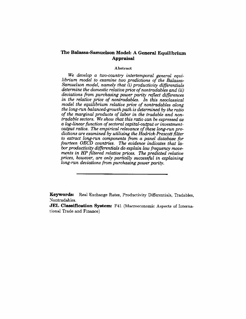
The Balassa-Samuelson Model: A General Equilibrium Appraisal

Abstract

We develop a two-country intertemporal general equilibrium model to examine two predictions of the Balassa- Samuelson model, namely that (i) productivi& differentials determine the domestic relative price of nontradables and (ii) deviations from purchasing power parity reflect differences in the relative price of nontradables. In this neoclassical model the equilibrium relative price of nontradables along the long-run balanced-growth path is determined by the ratio of the marginal products of labor in the tradable and nontradable sectors. We show that this ratio can be expressed as a log-linear function of sectoral capital-output or investment- output ratios. The empirical relevance of these long-run predictions are examined by utilizing the Hodrick-Prescott filter to extract long-run components from a panel database for fourteen OECD countries. The evidence indicates that la- borproductivity differentials do explain low frequency move- ments in HP filtered relative prices. The predicted relative prices, however, are only partially successful in explaining long-run deviations from purchasing power parity.

Keywords: Real Exchange Rates, Productivity Differentials, Tradables, Nontradables. JEL Classification System F41 (M acroeconomic Aspects of Interna- tional Trade and Finance)

Balassa-Samuelson in General Equilibrium 2

“Unless very sophisticated indeed, PPP is a misleadinglypre- tentious doctrine, promising us what is rare in economics, de- tailed numerical predictions. ” [ Paul Samuelson (1964)l

I. Introduction

In two seminal papers, Balassa (1964) and Samuelson (1964), independently argued that labor productivity differentials between tradable and nontradable sectors will lead to changes in real costs and relative prices,’ bringing about divergences in exchange rate adjusted national price levels. In the last thirty years this insight has been the guiding principle for most theoretical and empirical research on real exchange rates.

Several different predictions of the Balassa-Samuelson model have been explored in the literature.2 Some empirical studies have focused on Balassa’s finding that real exchange rates bear a strong positive relationship to the level of output per-capita across countries. Others examine the relevance of sectoral inflation differentials in explaining differences in real exchange rates. 3 Furthermore, several theoretical papers have focused on the determinants of the equilibrium relative price of nontradables in intertemporal models (Dornbusch, 1983; Greenwood 1984).

However, surprisingly, little empirical work has been carried out on developing intertemporal equilibrium models to investigate the predictions of the Balassa-Samuelson model. Exceptions are Rogoff (1991) and Obstfeld (1993). Obstfeld provides evidence of deterministic trends in real exchange rates for Japan and the United States. He develops a small open economy model with unbalanced growth to capture this important stylized fact. Our analysis differs from his in that we model a two-country world with balanced-growth in which long-run relative price differentials reflect differentials in factor productivity growth.4 For the empirical analysis we focus on differences across countries in long-run levels of real exchange rates and domestic relative prices of nontradable goods. Thus, unlike Obstfeld (19931, we are concerned with the cross-sectional implications of the Balassa-Samuelson model rather than its time series implications.

In a closely related strand of the intertemporal equilibrium literature, Stockman & Tesar (1990) and Mendoza (1992) have studied the


quantitative implications of multisector equilibrium models of the business cycle. The authors use numerical methods popularized in the real business cycle literature to evaluate the role of productivity shocks and terms-of-trade disturbances in determining the cyclical properties of the relative price of nontradables and the real exchange rate, In a recent contribution to this literature, Backus & Smith (1993) derive closed-form solutions linking deviations from purchasing power parity (PPP) and real interest parity to international consumption patterns. They use a two-country general equilibrium exchange economy to examine the possibility that nontraded goods may explain the persistent deviations from PPP observed in the data.

This paper contributes to the empirical literature analyzing real exchange rates from a general equilibrium perspective. Our objec- tive is to examine two basic propositions of the Balassa-Samuelson model, namely that: (i) productivity differentials determine the domestic relative price of nontradables and, (ii) productivity differentials explain deviations from PPP. We carry out the analysis in the context of a two-country dynamic general equilibrium model. We derive the Balassa-Samuelson propositions as long-run implications of the model and obtain closed-form solutions for the relative price of nontradables and the real exchange rate. This is done by imposing the constraints required for balanced long-run growth driven by labor- augmenting (Harrod-neutral) technological progress.

We show that along the long-run balanced-growth path, the relative price of nontradables is determined by the ratio of the marginal products of labor in the tradable and nontradable sectors. This ratio can be expressed as a log-linear function of the investment-output ratio in the tradable sector. The investment-output ratio is shown to be a function of exogenous parameters describing preferences and technology. We then derive three empirically implementable equations from this dynamic general equilibrium version of the Balassa-Samuelson model. The empirical tests take into account the long-run nature of the Balassa-Samuelson model by extracting low frequency components from time series for 14 OECD countries with the Hodrick-Prescott (1980) filter. The empirical tests also exploit the panel structure of the data.

The empirical evidence we provide suggests that low frequency differences in relative labor productivities do explain differences in long- run relative prices in our sample of OECD countries. We conclude


that the first proposition of the Balassa-Samuelson model is consistent with the long-run implications of the balanced-growth general equilibrium model developed in this paper. We then follow Balassa (1964) and examine the extent to which the theory can explain low frequency deviations from PPP observed in the data. The results suggest that while relative labor productivity differentials do explain the long-run behavior of the domestic relative price of nontradables, the relative price of nontradables is far less successful in explaining observed cross- country differences in long-run CPI-based and GDP deflator-based real exchange rates. In our equilibrium model this negative result can be attributed to the failure of PPP in tradable goods; or to a rejection of either the constant-elasticity forms of the production and utility functions or the balanced-growth constraints.

As a by-product of our analysis we are able to clarify two theoretical results that are important in assessing the findings of some empirical studies of the Balassa-Samuelson model. First, the proposition that sectoral labor productivity differentials are the only determinants of equilibrium domestic relative prices is, in general, only a long-run im- plication of neoclassical models. We show that in the short-run, the ratio of marginal products of labor determines only the supply of nontradable goods relative to tradable goods. Demand is determined by the households’ marginal rate of substitution between the two goods. Thus, the short-run determination of the equilibrium relative price of nontradables cannot be studied without modeling the households’ optimization problem. This result casts doubt on empirical studies of the Balassa-Samuelson model that only consider the supply-side and time series properties of the relative price of nontradables, without distin- guishing between the long- and short-run components of the data.

Second, a key finding of the original Balassa paper is that there is a positive relationship between aggregate output per head and the real exchange rate (or the relative price of nontradables). However, the theoretical analysis shows that in the long-run, it is the ratio of marginal products of labor that determines the relative price of nontradables. Therefore the Balassa-Samuelson model cannot predict how aggregate output per-capita should relate to domestic relative prices. This holds even if it is assumed that sectoral technologies are such that average and marginal products are proportional to each other and that population is a good proxy for labor services or hours worked. We conclude that, although the observed positive relationship between aggregate


output per head and the real exchange rate (or the relative price of nontradables) remains an important stylized fact, it cannot be derived from the theoretical principles underlying Balassa and Samuelson’s original formulation.

The paper is organized as follows. In section 2 we outline the theoretical framework and establish the Balassa-Samuelson propositions as steady-state implications of a standard dynamic neoclassical model. In section 3 we discuss data analysis and filtering issues. In section 4 we provide the empirical results. Section 5 presents some concluding remarks. -

II. The Theoretical Framework

In this section we describe the structure of our two-country, two- sector, intertemporal general equilibrium model. The model we examine is similar to that developed by Stockman and Tesar (19901, but differs in that our analysis focuses on the long-run rather than on business cycle frequencies. The conditions we derive for the long-run behavior of the relative price of nontradables are robust to alternative specifications within the class of multisector intertemporal equilibrium models of the open economy. In particular, our results hold for models with or without complete contingent claims markets and with or without distortionary taxes (Mendoza and Tesar 1993).

Consider a two-country world economy where households in each country consume tradable and nontradable goods and supply labor services to firms producing those goods. Households formulate optimal intertemporal plans to maximize expected lifetime utility. Firms produce tradable and nontradable goods by hiring the services of labor and capital and by combining them according to Cobb-Douglas technologies subject to stationary productivity disturbances. Households and firms are free to trade goods, equity, and financial assets inter- nationally. For notational clarity we only describe the characteristics of preferences and production in the home country. Foreign country characteristics are symmetric and, where necessary, identified by an asterisk.


A. Firms

Firms in the home country produce two types of goods tradable (T) and nontradable (NT) according to the following constant returns to scale Cobb-Douglas technologies:

YtT = F(K,T, N,T) = A~(XtN,T)aT(K,T)l-aT 0 5 cxT 5 1, (1)

yt NT = F(K,NT, N,NT) = A~T(&,~T)aNT(,;T)l-aNT 0 5 aNT < 1,

(2) where the production function, F(.), in each sector is assumed to be con- cave, increasing and twice continuously differentiable. Y;, i = T, NT is the output of tradable and nontradable goods at time t respectively; Kj, i = T, NT are the stocks of physical capital allocated to the production of tradable and nontradable goods at time t. Factors of production are assumed to be perfectly mobile across tradable and nontradable sectors and may be owned by households in either country. Nj, i = T, NT represents labor inputs required for the production of each good at time t, Xt is an index of Harrod-neutral labor-augmenting technological progress at time t and AZ, i = T, NT are stochastic productivity disturbances.5 Total factor productivity in each sector is given by:

c9T = A;(Xt)aT,

eNT = A,NT(&)aNT. t (4 The stationary productivity shocks induce fluctuations of macroeconomic variables around long-run deterministic trends6 These long-run trends are identified by imposing the balanced-growth conditions dis- cussed in King, Plosser, and Rebel0 (1988) when growth is driven by exogenous, labor-augmenting technological progress as in (1) and (2). Technological change evolves over time at the rate y (where y is the rate of growth of labor-augmenting technological change, i.e., the aggregate growth rate). For conventional preferences and technology this results in balanced-growth for all components of aggregate demand. Moreover, from (3) and (4) it follows that the total differential in total factor productivity growth that has played a key role in previous studies of the Balassa-Samuelson model is:


(5)

where G, xt$ y=-=- xtT xtT

and

where E is a stationary random process. Thus, for a given rate of balanced growth (y), the differential in total factor productivity is determined by the difference in labor income shares.

It is well known that with labor-augmenting technological progress the model exhibits steady-state growth. Therefore, a transformation is required to render the representative households optimization problem stationary. This transformation is achieved by deflating all variables (except labor and leisure) by the index of technological progress Xt.7

The first order conditions for the firm’s optimization problem, given the rental rate for capital rt and the wage rate for labor wt in each sector, yield the following zero-profit conditions:

f (k,NT, N,NT) = ,TTkyT + wyTN,NT

(6)

(7) where f(a) and kf, i = T, NT represent the transformed (detrended) production functions and capital stock, respectively. rf , i = T, NT is the rental rate for capital in the tradable and nontradable sectors at time t and w;, i = T, NT are real wages in each sector at time t.

The economy household with a

B. Households

is inhabited by an infinitely lived representative time separable utility function defined over the con-

sumption of tradables, nontradables and leisure. The household max- imizes the discounted sum of expected lifetime utility.

E F@u(c:, ctNT, Lt) 1 o<p<1, (8) t=o


where E is the expectations operator conditioned on the time t information set; p is the subjective discount factor; CT and cyT are the consumption of tradables and nontradables at time t respectively and it is the time devoted to leisure. The instantaneous utility function is twice continuously differentiable in each of its arguments.

We assume a constant elasticity of substitution (CES) instantaneous utility function:

u(*) = I R(CpJ + (1 - n,c,fiT,-r] =;;? Lr]l-u

1-C 7 (9)

where R is the share of tradables in consumption; l/l + /I is the elasticity of substitution between tradable and nontradables and w is the elasticity of leisure.

Households maximize utility subject to the budget constraint:

Pt NT,--+cT = [ $kF + +k,F + pt NTdNTktNT 1 [ + zo:Nr + pFTwyTNtNT 10)

1

y [ k$ + k$ + ppTkNT] + (I- 6) [k: + k: + p,‘k,‘]

--y&h+1 + bt,

and the normalized time constraint:

(11) where pyT is the relative price of nontradables, ktH, kr and kyT are the stocks of physical capital owned by households in the home country in the domestic tradables sector, the foreign tradables sector and the domestic nontradables sector respectively. Capital in both sectors is assumed to depreciate at the same rate 6.

Households accumulate net foreign assets, b, that yield the world interest rate it. R is the inverse of the real gross rate of return paid on international bonds. Thus we assume a financial market structure in which countries trade equity and noncontingent bonds and therefore insurance markets are incomplete. The household’s problem, therefore incorporates the period-by-period constraint (10) instead of the present value of wealth typical of complete market models.8

For the transformation procedure to produce stationary equilibrium allocations that correspond to nonstationary, balanced-growth equilibrium allocations, two additional adjustments are required. First,


the discount factor must be transformed so that b = p . 7l-O where p = l/l + p is the rate of time preference and u is the coefficient of relative risk aversion.g Second, it is required that y be introduced as a multiplicative factor in the accumulation of capital and bonds in the budget constraint.

C. Competitive Equilibrium

In a competitive equilibrium for this world economy, home and foreign households maximize utility, home and foreign firms maximize profits and the goods, services, and financial asset markets clear. In particular, the domestic market for nontradables in each country as well as the world market for bonds and tradable goods clear. The competitive equilibrium is characterized by allocations of consumption, labor supply, capital and international bonds that satisfy the following optimality conditions in the home country:

ul(t) NT

Uz(t)=pt ’

U3(t) T

vi(t) = wt ’

U3(t) NT

vz(t)=“” ’

yRtul(t) = PE [W + 111 T

(12)

(13)

(14)

(15)

yul(t) = PE [Ul(t + 1) [& + 1 - 6]] ,

-/Ul(t) = PE [UI(~ + 1) [rtT+tl + 1 - 6]] ,

YPt NT~l(t) = ,f3E [p&;Lr,(t + 1) [$; + 1 - 6]] 7

rF = fl(kf-7 N,T),

wf- = f*(& N,T),

rt NT = fl(q, $1,

(1’3)

(17)

(18)

(19)

(20)

(21)


‘Wt NT = f+T, NT).

The market-clearing conditions are: (22)

f(kyT, N,NT) = cyT + -yk~~ - (1 - 6)k,NT, (23)

f(kyT*, N,NT*) = cyT* + y*ktN+T - (1 - S)kyT*, (24)

f(k;, NT) + f(@, N,T*) = CT + cp + yk,T,, (25) -(l 2 S)k,T + y*lc,T,, - (1 - ap,

bt + b; = 0. (26)

where vi, i = 1,2,3 is the partial derivative with respect to the first (cT), second (cNT) or third (L) arguments of the utility function. The corresponding conditions in the foreign country and the budget constraints are also part of the set of optima& conditions describing world equilibrium. Conditions (12)-(22) have the usual interpretation in terms of marginal productivities and rental prices of inputs.

Of considerable importance in our analysis of the Balassa- Samuelson model are equations (12)-(14) and(U)-(22), that determine the equilibrium relative price of nontradables. Equation (12) states that from the demand-side, the equilibrium relative price of nontradables at time t is equal to the marginal rate of substitution between tradable and nontradable goods. By dividing (14) by (13), substituting the result in (12), and displacing the rental prices of labor with the marginal products as stated in (20) and (22), one can show that from the supply-side the equilibrium relative price of nontradables at time t is the ratio of the marginal products of labor in the tradable and nontradable sectors,

This static characterization of the relative price of nontradables in terms of the ratio of the marginal products of labor is the principle emphasized by Balassa and Samuelson. However, in world general equilibrium both demand- and supply-side conditions must be satis- fied by the market-clearing relative price of nontradables. Moreover, these two conditions are not independent of the rest of the equilibrium system. In deterministic form (18) is an Euler condition linking the intertemporal marginal rate of substitution to the change in the


relative price of nontradables over time. This Euler condition intro- duces intertemporal income and substitution effects in the determination of the relative price of nontradables at date t. This means that optimal intertemporal plans concerning consumption and investment affect atemporal decisions regarding allocations of consumption across tradables and nontradables and of capital and labor across sectors; hence affecting the relative price of nontradables.

D. The Long-Run Price of Nontradables

In general, the original Balassa-Samuelson principle is only a characterization of supply-side determinants of the relative price of nontradables. In this section we show that the Balassa-Samuelson principle can be interpreted as an equilibrium outcome along the long-run balanced-growth path.

To establish the Balassa-Samuelson principle as a long-run equilibrium outcome we proceed by assuming the random shocks to the production technologies are stationary and that certainty equivalence holds. This, enables us to examine the long-run balanced growth world equilibrium by focusing on the model’s deterministic stationary state. In this steady-state, the equilibrium relative price of nontradables reduces to expressions closely related to the Balassa-Samuelson framework.

Consider the supply-side equilibrium condition that equates the relative price of nontradables to the ratio of the marginal products of labor, in the tradable and nontradable sectors, within a country:

pNT = f2 (k& NtT) f2 (kt NT, NtNT 1’

Exploiting the fact that Cobb-Douglas production functions have the property that output per man-hour is a monotonic transformation of the capital-output ratio, (y/N) = (k/y)“-“)I* enables us to write the relative price of nontradables as:


Thus, (27) is the supply-side condition that states that the relative price of nontradables is a function of sectoral labor shares and sectoral capital-output ratios. Note that from (27) the relative price of nontradables is higher the higher is output per man-hour in the tradable goods sector relative to the nontradable goods sector. Therefore the theory, as developed here, cannot predict how aggregate output per-capita re- lates to domestic relative prices. lo Even if it is assumed that technology is such that average and marginal products are proportional to each other, as in the Cobb-Douglas case, and that population is a good proxy for labor services or hours worked, it is the ratio of sectoral output-per- capita levels that determines the relative price of nontradables and not the aggregate level of output.

From (16) and (18) it follows that in a deterministic stationary equilibrium with perfect sectoral capital mobility, the marginal products of capital in the tradable and nontradable sectors are equalized:

fl (ky, N,T) = fl (k,NT, N,NT), with Cobb-Douglas production functions this relationship reduces to:

Equation (27) can therefore be rewritten to express the relative price of nontradables as a function of the labor shares in both sectors and the capital-output ratio in the tradables sector:

Up to this point, we have derived expressions for the relative price of nontradables that depend on capital-output ratios and represent either the supply-side condition (27) or that condition jointly with the steady-state equality of sectoral marginal products of capital (28). To argue that these conditions explain equilibrium allocations along the balanced-growth path, we need to establish that capital-output ratios are exogenously determined by structural parameters. We do this by imposing steady-state conditions on all of the equations (12)~(22). Af- ter manipulation of (16), in long-run balanced-growth equilibrium the capital-output ratio in the tradables sector is:


ktT j(1 - crT)

z= y-j(l-6)’ (29)

This equation incorporates the steady-state equality of the intertemporal marginal rate of substitution in consumption and the real rate of return on capital (net of depreciation) required to produce balanced- growth at the rate y in the components of aggregate demand.

What emerges from the analysis, at this point, is that in long-run growth equilibrium the capital-output ratio in the tradables sector is determined by exogenous structural parameters, ,0,7, CJ, CXT, 6. There- fore, at low frequencies (27) and (28) can be interpreted as expressions that determine the equilibrium relative price of nontradables and not simply the supply-side of the economy. The steady-state definition of the investment rate is:

iT yT = I-Y - (I- a>] $7

working with (29) and the steady state definition of the investment rate yields an alternative representation of the equilibrium relative price of nontradables as a function of the investment rate:

or as a function of deep structural parameters:

Finally, note that the expressions we have derived for the equilibrium relative price of nontradables in (27), (28) and (30) are consistent with those from earlier studies of the Balassa-Samuelson model that emphasize sectoral differentials in factor productivity growth.ll This is evident from the fact that in this model, given capital-output or investment-output ratios, the relative price of nontradables is determined by the relative size of aNT and cuT. These two parameters in turn determine the differential in sectoral total factor productivity growth given in (5).

Balassa-Samuelson in General Eauilibrium 14

E. The Long-Run Real Exchange Rate

In this subsection we link real exchange rates to the equilibrium relative prices of nontradables. We establish the connection between the model’s equilibrium relative price of nontradables and the real exchange rate by following the convention of the intertemporal equilibrium literature.12 The convention is to proceed by noting that the households problem has a dual representation with an expenditure function P&t where Ct is a composite consumption good represented by, Ct = [R(cT)+ + (1 - s2)(c~T)-~]-1/~, and Pt is the price index of the composite consumption good represented as,

Define the real exchange rate as st = Pt/Pt.13 Then, if the law of one price holds for tradable goods, the real exchange rate is expressed as:

From this expression it is evident that the real exchange rate is a function of the relative price of nontradables in the two countries. In long-run, balanced-growth, equilibrium the real exchange rate is therefore a function of the same structural parameters (of preferences and technology) that determine the ratio of the marginal products of labor (in tradable and nontradable sectors) that we showed earlier determine the relative price of nontradables.

Assuming Cobb-Douglas preferences, i.e., (l/l + /I = l), enables us to conveniently express the real exchange rate for empirical implemen- tation as:

(~*)“*(l_ Q*)l-w St =

f-$2(1 - q1-i-2 (32)


III. Data Analysis and Filtering

Estimating (2’7), (28) (30) requires data on the relative price of nontradables, the investment-output ratio in the tradable sector and the capital-output ratios in the tradable and nontradable sectors. These variables do not exist in ready form, so the first task was to construct these variables from existing sources.

As our focus is on the cross-country properties of the data, we constructed a panel dataset. The dataset provides a rich source of cross- country information and consists of annual data for 14 countries14, 20 sectors15 spanning 1970-85 and was obtained from the OECD inter- sectoral database. The database includes information on sectoral real and nominal valued added capital stock, investment, employment and factor returns for each of the 20 sectors. From this database we constructed series for the relative price of nontradables, the investment- output ratio in the tradable and the capital-output ratio in nontradable sector for each country in our sample.

In order to construct the required data, the first issue is to de- cide which sectors are to be considered tradable and nontradable. We choose DeGregorio, Giovannini and Wolf’s (1994) classification scheme. This scheme is based on the ratio of the actual shares of total exports to total production across all 14 countries for each sector. This results in a sector being classified as tradable if more than 10% of total production is exported. I6 The 10 % threshold classifies agriculture, mining, all of manufacturing and transportation as tradables with the remaining sectors classified as nontradables. Annual data on real exchange rates based on trade weighted consumer price indices (CPI) were obtained from the IMF International Financial Statistics while GDP deflator- based real exchange rates were taken from Micosi & Milesi (1993).

We decided to extract the long-run growth component of the data before estimation for the following two reasons. First, we have shown that the Balassa-Samuelson predictions are long-run equilibrium implications. To be consistent with the theory, any tests of the predictions of our model must be based on the long-run components of the data. In principle, the constant rate of Harrod-neutral technological progress in our treatment of the Balassa-Samuelson model should enable us to distinguish between the long-run and short run components of the data.17

Second, it is well known that employment adjusts gradually to


changes in output and as a result labor productivity rises in an economic upturn and declines in a downturn. By extracting the growth component from the data, we isolate the factors that are more closely related to long-run labor productivity and abstract from short-run cyclical changes that may bias the results.

Several statistical procedures have been used to filter data in macroeconomic analysis. The most common ones are the linear-trend filter, the Hodrick-Prescott (HP) filter, the Beveridge-Nelson filter and random-walk detrending (Canova & Dellas 1993). Unfortunately, a consensus on the appropriate use of filters in macroeconomic analysis does not exist. However, Baxter (1991) and Singleton (1988) have argued that the choice of filtering procedure should be governed by the theoretical model at hand. We find their arguments compelling and choose two filters: the linear-trend and HP-filters that are consistent with our version of the Balassa-Samuelson model (i.e, deterministi- tally trending variables uncorrelated with the cyclical components of the data) as candidates for extracting long-run trends from the data.

The linear-trend filter removes a deterministic linear trend from the data and is attractive for its simplicity. However, the simplicity of the linear-trend filter presents a drawback when applied to highly nonstationary processes such as exchange rates and relative prices. To confirm that the data does exhibit nonstationarity, we carried out Dickey-Fuller and Augmented Dickey-Fuller stationarity tests. As expected, the tests fail to reject the presence of unit roots in all three of the data series.‘*

The HP-filter has certain attractions relative to the linear-trend filter. Like the linear-trend filter, the HP-filter assumes that the cyclical and growth components of the data are uncorrelated. However, unlike the linear-trend filter, the HP-filter will render stationary any integrated process up to fourth order (King & Rebel0 1993). Furthermore, the HP-filter permits the data generating process to have a deterministic as well as a stochastic growth component.

Figure 1 plots the actual observations and the HP-filtered trends of the relative price of nontradables, the investment-output and capital- output ratios in tradables and the capital-output ratios in nontradables for Germany. Visual examination of Figure 1 suggests that linear trends are not likely to differ significantly from the HP-filtered trends. We confirmed this by plotting both filters. While the two filtering procedures are remarkably similar for some variables like the


investment-output ratio the HP-filter captures a slow moving trend that the linear trend filter misses. Given these results, we decided to use the HP-filter in the empirical analysis reported in the remainder of the paper.lg INSERT Figure

A striking feature that is evident from Figure 1 is the smoothness 1 here of the trend component that emerges from the HP-filtering procedure. Harvey & Jaeger (1993) argue that to avoid blind application of the HP-filter, the assumption of a smooth deterministic trend should be empirically verified by estimating a structural time series model:20

Yt = pt + rt + Et t = l...T

where it is the series; pt is the trend; It is the cycle and Et is a random error term. The trend is:

,w = /-Q-l + k-1 + 77 rlt N NO, g,“,

Pt = A-1 + <t tit N NO, $,

where Pt is the slope parameter and & and qt are independent and normally distributed white noise.

The cyclical term is stochastic and assumed to be generated by

rt = p cos X,rt-1 + p sin &I,*_, + xt

r; = -psinX,rt-l + PCOS x,r;-, + Z;

where p is a damping factor such that 0 5 p 5 1,X, is the frequency of the cycle. xt and x: are both normal and identically distributed disturbances with mean zero and variance gp. The random error term is also normal and identically distributed with mean zero and variance ~2 and all three components are assumed to be independent of each other.

Ifaf = 0 the trend reduces to a random walk with drift. Further- more if 614 = 0, the trend becomes deterministic, that is Ut = ~0 + Pt. When a; = 0, but c$ > 0 the trend component is relatively smooth. Therefore, whether the trend component is deterministic and well represented by a smooth process can be verified by testing whether ai = 0.

We carried out maximum likelihood estimation of the parameters of the structural model for each of the 14 countries for 4 variables (the

c

t

t

t B


real exchange rate, the relative price of nontradables, the investment- output ratio in tradables and the capital-output ratio in nontradables) to determine whether this restriction was supported by the data. The results indicate the deterministic smooth trend assumption is supported by the data for 10 of the 14 countries for all 4 variables since al7 = OB21 The remaining 4 countries had values of al7 that were small ranging from 1-4 but with values of Ge = 0.22 The fact that &e = 0 suggests that even for these 4 countries the series decomposes into a smooth trend and cycle. Finally, plots of the trend component from estimates of the structural model for the 4 countries suggest that trends from the structural model have similar features to those from the HP- filter. These results are consistent with Obstfeld (1993) who provides evidence of deterministic trends in real exchange rates for the US and Japan. 23

IV. Empirical Results

The empirical analysis is structured around two questions. First, do long-run relative labor productivities explain long-run relative nontradable prices? Addressing this question will enable us to evaluate the Balassa-Samuelson model as a theory of the determination of domestic relative prices. Second, do cross-country differences in long-run relative nontradable prices explain cross-country, long-run, real exchange rate differentials? Addressing the second question enables us to determine the extent to which the Balassa-Samuelson framework can be considered a theory of real exchange rates.

A. Evidence on the long-run Relative Price of Nontradables

Having derived closed-form solutions for the long-run relative price of nontradables; our empirical strategy is to confront the theory with the data in the most parsimonious manner possible. In reassessing the Balassa-Samuelson model we therefore purposefully refrain from adding additional right-hand-side variables not derived from the model to the regressions. The tests we carry out are joint tests of the theory and the assumption of Cobb-Douglas technology.

The log-linear form of the nontradable price equations for country j derived in (27), (28) and (30) can be conveniently summarized for


estimation as:

$T = aoj + ~rlky,Tt + a2kyJTT + ejt, (I) g = Yoj + rlkV$ + ejt, (II) $T = ql)j + qliYzT + ejt. (III)

for j = 1,2, . . , M countries and t = 1,2, . . . , T time periods, where pNT is the log of the relative price of nontradables; kyT is the log of the capital-output ratio in tradables; kyNT is the log of the capital-output ratio in nontradables; iyNT is the log of the investment-output ratio in tradables and ejt are random disturbances. For easy reference these three specifications will henceforth be referred to as specification (I), (II) and (III) respectively.

The theory requires the coefficient on the capital-output ratio (02) in nontradables to be negative and the coefficient on the capital-output ratio (cri) in the tradables sector to be positive in (I). With respect to (II) and (III) the theory does not impose constraints on the coefficient on the capital-output ratio in tradables (71) or on the coefficient on the investment-output ratio in tradables (vi). However, if aT > aNT, as data on labor income shares suggests,24 then both yi and 71 should be negative. Moreover, the model also implies that the cross equation restrictions yi = 71 = ai+ CY:! should hold.

Table 1 provides least squares estimates of a pooled (total) regression of equations (I), (II) and (III) . Equation (I) performs particularly well in several respects. First, the coefficients are statistically significant and of the correct sign. Second, (yT > aNT is implicit in the results although the implied shares aT = 0.81 and aNT = 0.78 are higher than direct measures suggest. Finally, equation (I) explains nearly one quarter of the variations in the relative price of nontradables. INSERT Table

In contrast the results from estimating (II) and (III) are less favor- 1 here able. The coefficient estimates of yi and 71 are not statistically different from zero and the explanatory power of the regressions is very low. From (I) it follows that cui + CQ = -0.038. However, the t-ratio for the null hypothesis that 71 and 71 are not different from ai +cu2 = -0.038 is 3.2 and 4.1, respectively. Thus although the data do not provide precise estimates of yi and 71, the cross equation restrictions yi = 71 = (pi+ cr:! cannot be rejected.

A possible reason for the failure of the pooled regressions (I, II) is that in performing least squares regressions with all MT observations


we have assumed that the intercept and slope coefficients take values common to all cross-sectional units. If this assumption is not valid, the pooled least squares estimates may lead to false inferences. To investigate whether the regression coefficients are the same for all countries we carry out several homogeneity tests.

Our strategy is to determine whether the slopes and intercepts si- multaneously are homogeneous among different countries at different times. Then we test if the regression slopes are collectively the same. Under the assumption that the errors ejt are independently normally distributed over j and t with mean zero and variance a:, we construct F tests of the above linear restrictions.

Table 2 presents the results of tests for the homogeneity of regression slope coefficients and homogeneity of the regression intercept coefficients. In hypothesis 1 (same slopes, same intercepts) the F ratio is significant so we reject the hypothesis of complete homogeneity. Hy- pothesis 2 (same slopes but different intercepts) is also rejected, suggesting that the slope coefficients are also different across countries. We interpret the failure of these tests as suggesting that sectoral labor shares; which are the determinants of intercept and slope estimates in (I), (II) and (III); diff er across countries or groups of countries. Later, we show how estimation performance improves if we group countries according to relative labor shares implicit in the intercept estimates. INSERT Table

Next, we decompose the pooled regression estimates into “ within ” 2 here. and “ between ” components for two partitions of the sample. Panel A in Table 3 is for the full sample while panel B is based on subsamples for 1970-77 and 1978-85. The between component represents the output of an OLS regression based on the means of each country’s time series, while the within component is the outcome of a fixed-effects model. By proceeding in this manner we can determine the contribution of each of the two components to the outcome of the total regression. INSERT Table

The results of the decomposition are reported in Table 3. The 3 here. weights (K) on the between estimates indicates that almost 90 % of the variation in the pooled estimates is due to heterogeneity across countries. Thus the favorable results obtained with the pooled regressions reported in Table 1, particularly for equation (I), can be viewed as reflecting mainly cross-country differences in trend behavior, rather than within country time series patterns. This result is robust to the specification of two subsamples. Moreover, coefficient estimates are generally stable for the sample break down examined.


To explain the difference in performance between (I), (II) and (III) recall that in deriving (II) and (III) we impose the equilibrium condition that equates the marginal products of capital in the tradable and nontradable sectors. We simplify this equality with the conditions required for balanced-growth in the model. Particularly the assumption that the domestic relative price of nontradables is constant in the long-run (at levels that differ across countries depending on total factor productivity growth). Therefore, our results may reflect the fact that these requirements are too demanding for this fragile dataset. To explore this hypothesis of a cross equation restriction implied by the theory: yi = (ai+ crp) we estimate (I) and (II) using Zellner’s seemingly unrelated regression technique. The Wald statistic reported in Table 4 states that we cannot reject the restriction. Failure to reject the restriction should be interpreted with caution as the t-ratios are small, implying the standard errors are large, and therefore that the test has low power. A possible interpretation of these results is that there is some degree of sectoral capital mobility but that it is less than perfect. Measurement errors in the capital stock may be another reason for the poor performance of (II). INSERT Table

We next attempt to determine whether there are any cross-country 4 here. patterns related to productivity that can be exploited for estimation. To do this we use parameter restrictions related to the differential of total factor productivity growth from the Balassa-Samuelson model given in (5). In particular, recall that in steady-state, balanced-growth equilibrium, productivity growth in the tradables sector will be faster than that in the nontradables sector if CYT > CYNT. However, note that the intercept of (I) is aT/, NT. This is a measure of the magnitude of the differential in productivity growth. Following this observation we use the parameter estimates from (I) to group countries by the degree to which they behave consistently with the Balassa-Samuelson hypothesis.

The individual country estimates reveal a group of countries for which the intercept is greater than 1, another group with intercepts less than 1 and an intermediate group with intercepts close to 1. Heuristically, countries with an intercept greater than 1 should behave more like the Balassa-Samuelson model predicts, and countries with an intercept less than 1 should behave less like the model predicts. We therefore classified the countries as low-Balassa, medium- Balassa or high-Balassa with 4 countries in the low-Balassa group:


USA, Denmark, Germany and Finland; 6 countries in the medium- Balassa group: England, Australia, Sweden, Belgium, Norway and France; and 4 countries in the high-Balassa group: Japan, Canada, Italy and the Netherlands.25

After grouping the countries by this criterion we estimate a fixed- effects model for equation (III). The results reported in Table 5 are striking. The explanatory power of the regression improves remarkably from the low-Balassa to the high-Balassa countries. The coefR- cients on the investment-output ratio for all countries are of the correct sign and statistically significant.26 INSERT Table

Having established that (I) and (III) are reasonable empirical rep- 5 here. resentations of the Balassa-Samuelson model we address some robust- ness issues. So far the entire analysis has been carried out with pooled and fured-effects models. fixed-effects is the appropriate statistical model when the cross-section of countries represents the entire uni- verse of interest. However, recall that we use data for 14 of the 24 OECD countries. This may raise some doubt as to the appropriateness of the fmed-effects model in the present circumstances. If one views the country-specific effects as randomly distributed across cross-sectional units then the appropriate methodology is a random-effects model.

We estimate a random-effects model by adopting the following component structure for the disturbances: ejt = tj + vjt, where <t are the country specific effects, and Vjt are idiosyncratic shocks. If the right- hand-side variable is uncorrelated with both ejt and vjt and vjt is uncorrelated across time, then the standard variance components gener- alized least squares (GLS) estimates are appropriate.

The results of the random-effects model estimated using GLS are reported in Table 6. While (III) performs well with coefficients that are statistically significant and of the correct sign, (I) and (II) yield wrong sign coefficients. To alleviate concerns about whether fured or random- effects is the appropriate model we apply the Hausman specification test (Hausman 1978). The test resoundingly rejects the random-effects specification suggesting that the fixed-effects estimates are robust. INSERT Table

In section 3 we established the appropriateness of the smooth de- 6 here. terministic trend assumption imposed by the HP-filter. To verify that our empirical results are robust to the HP-filtering procedure we carry out the entire estimation using the linear-trend filter. The result of estimating (III), presented in Table 7, shows there is little difference between the two procedures.27 INSERT Table

7 here.


In short, our results suggest that the Balassa-Samuelson proposition that relative marginal products of labor explain domestic relative prices is well supported by the data in the total and fixed-effects models of equations (I) and (III). Furthermore, our results are not sensitive to the HP-filter.

B. Evidence on the Long-Run Real Exchange Rate

The evidence provided above supports the appropriateness of the Balassa-Samuelson model as a theory explaining long-run, cross- country differences in domestic relative prices. The next issue we address is the extent to which these differences can explain differences in long-run real exchange rates. We focus on a log-linear version of (32). Assuming 0: = 1 yields the following testable equation28

Sjt = 6Oj + slPjt NT + ejt, (IV)

forj = 1,2,..., M countries, and t = 1,2, . . . , T time periods, where pNT is the log of the relative price of nontradables, s is the log of the real exchange rate and ejt are random disturbances.

Due to data limitations we use two separate real exchange rate series. A CPI-based exchange rates series for all 14 countries but for only part of our sample period (197585) and a GDP deflator-based exchange rate series for the full sample period but for only 8 of the 14 countries. As in the previous analysis we extracted the long-run growth component from the data by using the HP-filter.

Table 8 presents least squares estimates of a simple pooled linear regression of the CPI-based real exchange rates on both actual measures of relative prices, i.e, (IVa), and the predicted relative prices estimated from (III), i.e (IVb), for all 14 countries for the period 197585. As expected, from (IVa), higher prices for the relative price of nontradables are positively associated with the real exchange rate. The coefficient estimates on the relative price of nontradables is positive though insignificant. In (IVb) the coefficient is statistically significant at the 10 % level in a one-tailed test. However, note that the explanatory power of both the actual and the predicted nontradables price specifications are extremely low. INSERT Table

We also estimate a fixed-effects regression to examine the cross- 8 here. country properties of this specification. The results reported in Table


9 show that the explanatory power is very high. This is because within country intercepts are very good at tracking HP trends. INSERT Table

Tables 10 and 11 repeat the previous exercise with GDP deflator- 9 here. based real exchange rates. Table 10 reports results for least squares estimates of a simple pooled regression using both actual relative prices and our predicted relative prices from (III) to explain the GDP deflator- based real exchange rates. None of the coefficient estimates are statistically significant and the explanatory power is still very low. With the fixed-effects regression (Table ll), the results remain poor. The explanatory power improves considerably for the same reason as above and the coefficients on the price of nontradables have incorrect signs with one of them being statistically significant.

Table 11 also reports estimates for the within and between regressions for GDP deflator-based real exchange rates. These results indicate that unlike nontradable prices (see Table 3) in which much of the variation in the pooled OLS estimates is due to heterogeneity across country units, much of the variability in GDP deflator-based real exchange rates is due to “within” country factors. It appears that while the panel structure of the data was helpful in explaining the relative price of nontradables, it is less helpful in explaining long-run real exchange differentials. INSERT Tables

Finally, aware of the limitations of our dataset and the fact that our 10, 11 here. decomposition of tradables and nontradables is at best a rough approximation we attempt to determine to what extent the inability of our relative price measure to explain real exchange rate behavior can be attributed to measurement errors. One, albeit limited way, to address this question is to use better quality data on tradables and nontradables from Kravis, Heston & Summers [1982] (KHS). So taking the following from KHS, (i) data on the prices of tradable and nontradable goods from Table 6.12 and (ii) their measure of the GDP-based real exchange rates (the exchange rate deviation index) from Table l- 2 for 1975 for 34 countries we estimate a least squares regression of the log real exchange rate on the log of the ratio of nontradable and tradable prices. The estimates from this carefully constructed dataset (t-statistic of 6.48 and an R2 of 0.65) suggest that there is a long-run equilibrium relationship between real exchange rates and the relative price of nontradables.

In conclusion, the results of the empirical tests of the second Balassa-Samuelson proposition suggest that, while international dif-


ferences in the long-run relative price of nontradables reflect differences in sectoral marginal products of labor as predicted by the theory, these differences explain only a small fraction of long-run deviations from PPP based on aggregate price indexes. One interpretation of this evidence is to cast doubt on the validity of long-run PPP for tradables. However, significant measurement error, as suggested by the estimates obtained from the Kravis-Heston-Summers data may account for our findings. Furthermore, the tests we conducted embody nested hypotheses regarding a balanced-growth neoclassical framework and constant-elasticity utility and production functions.

V. Concluding Remarks

In celebration of thirty years of the Balassa-Samuelson model, we have attempted to provide an appraisal of the static theory of BaI- assa (1964) and Samuelson (1984) by embedding it in an explicitly dynamic general equilibrium setting. Our appraisal of this celebrated model followed three stages. First, we derived two of the Balassa- Samuelson propositions as long-run, balanced-growth, implications of a two-country intertemporal equilibrium model. Second, we identified restrictions imposed on the cross-sectional, low-frequency behavior of the data implied by our model and thus derived testable predictions. Third, we constructed a cross-country sectoral database from existing OECD data and conducted econometric tests of the predictions of our model using panel data methods.

The empirical analysis suggests the Balassa-Samuelson proposition, that cross-country differences in long-run domestic relative prices of nontradables are determined by differences in the ratio of long-run sectoral marginal products of labor, cannot be rejected by the data. However, we also found that long-run relative prices (as measured in the data or as predicted by our regressions) are of little help in explaining long-run, cross-country differences in the level of real exchange rates measured with CPI- or GDP deflator-based exchange rates. Thus, while the Balassa-Samuelson general equilibrium model performs well as a theory of relative prices, it seems to be unable to account for trend deviations from PPP. This statement echoes Paul Samuelson’s quota- tion that prefaces the paper.

We conclude by pointing out some limitations of our work. On the


empirical side, further work is required to develop a higher quality sectoral database covering a longer period and for a larger panel of countries. On the theoretical side, while we have succeeded in ex- tending the static model to a dynamic setting, the simple deterministic neoclassical growth framework restricts our analysis to balanced- growth paths. Furthermore, an important assumption in our model is that Harrod-neutral technological progress expands at a constant rate. This assumption enables us to get a clear separation between trend growth and cycles and motivates the use of the HP-filter. However, such a clear separation fails if technological progress is stochastic or in models of endogenous growth. In a recent paper, Asea & Sturzenegger (1994) develop and test a Balassa-Samuelson type model based on an endogenous growth framework. Work along the lines carried out in this paper of developing robust general equilibrium restrictions that can be tested with the data will enhance our understanding of the en- during empirical regularities observed by Bela Balassa (1964) and Paul Samuelson (1964).


Appendix A

The Hodrick and Prescott [ 10901 filter is a two-sided filter that removes a trend that resembles a smooth curve drawn through the data. The HP filter defines a trend {q} for a series {yt} as the solution to the following optimization problem:

T T-l

@(Yt - ?I2 + x c [(P+1 - 9) - Tt - Q-1)12. t-1 t=2

(A. 34)

where x is a parameter which penalizes changes in the trend component. The larger the value of x the smoother the trend component. We chose x = 400 which is consistent with other studies that use annual data. We also experimented with X = 100 this value gave us no no- ticeable difference in results. All results reported in the text are for X = 400. We used the RATS version 4.02 procedure HPFILTER.SRC to compute the trend and checked our results against a routine written in GAUSS.


References

Asea, Patrick K. and Federico Sturzenegger, “ Real Exchange Rates and Endogenous Growth,” manuscript UCLA (1994).

and Enrique G. Mendoza, “The Balassa-Samuelson Model: A General Equilibrium Appraisal,” UCLA Working Paper No. 709 (1994).

Backus, David K. and Gregor W. Smith, “Consumption and Real Exchange Rates in Dynamic Economies with Nontraded Goods,” Journal of International Economics 35 (1993):297--316.

Balassa, Bela, “The Purchasing Power Parity Doctrine: A Reap- praisal,” Journal of Political Economy 72 (1964):584--96.

Baxter, Marianne, ‘Business Cycles, Stylized Facts and the Ex- change Rate Regime: Evidence from the United States,” Journal of International Money and Finance 10 (1991):71--88.

Bergstrand, Jeffrey H., “ Structural Determinants of Real Exchange Rates and National Price Levels: Some Empirical Evidence,” Amer- ican Economic Review 81 (1991):325--34.

Canova, Fabio and Harris Dellas, “Trade Interdependence and the International Business Cycle,” Journal of Economic Dynamics and Control 34 (1993):23--47.

Cole, Harold, “Financial Structure and International Trade,” Interna- tional Economic Review 29(2) (1988):237--59.

Dornbusch, Rudiger W., “Real Interest Rates, Home Goods and Optimal External Borrowing,” Journal of Political Economy 91 (1983):141--53.

DeGregorio, J&e, Albert0 Giovannini and Holger Wolf, “Inter- national Evidence on Tradables and Nontradables Inflation,” forthcoming European Economic Review (1994).

Friedman, Milton, A Theory of the Consumption Function, Princeton University Press, Princeton, NJ. 1957.

Frenkel, Jacob A. and Assaf Rabin, Fiscal Policies and the World Economy: An Inter-temporal Approach, MIT Press, Cambridge, MA. 1987.

Greenwood, Jeremy, “Non-Traded Goods, the Trade Balance and the Balance of Payments,” Canadian Journal of Economics 17 (1984):806- -23.

Harvey, Andrew and A. Jaeger, “Detrending, Stylized Facts and the Business Cycle,” Journal of Applied Econometrics 8 (1993):231--47.


Hausman, Jerry, “Specification Tests in Econometrics,” Econometrica 46 (1978):1251--71.

Hodrick, Robert and Edward Prescott, “ Post-War U.S. Business Cycles: An Empirical Investigation,” manuscript, Carnegie-Mellon University (1980).

Hsieh, David A., “ The Determination of the Real Exchange Rate: The Productivity Approach,” Journal of International Economics 12 (1982):355--62.

King, Robert G., Charles Plosser and Sergio T. Rebelo, “ Produc- tion, Growth and Business Cycles: I. The Basic Neoclassical Model,” Journal of Monetary Economics 21 (1988): 195--232.

and Sergio T. Rebelo, “ Low Frequency Filtering and Real Business Cycles,” Journal of Economic Dynamics and Control 17 (1993):207--31.

Kravis, Irving B; Alan W. Heston and Robert Summers, World Product and Income, Johns Hokins University Press, 1982.

-9- and ,“The Share of Services in Economic Growth,” in F.G Adams and B. Hickman (eds.), Essays in Honor ofLawrence R. Klein, MIT Press, Cambridge, MA. 1983.

and Robert E. Lipsey, “The Assessment of National Price Levels,” in Sven W. Arndt and J. David Richardson (eds.), Real- Financial Linkages among Open Economics, MIT Press, Cambridge, MA. 1987.

Marston, Richard C., “Real Exchange Rates and Productivity Growth in the United States and Japan,” in Sven W. Arndt and J. David Richardson (eds.), Real-Financial Linkages among Open Economies, MIT Press, Cambridge, MA. 1987.

Mendoza, Enrique G., “The Terms of Trade and Economic Fluctua- tions,” IMF Working Paper No. WP--92--98 (1992).

and Linda L. Tesar, “ Supply--Side Economics in an Integrated World Economy,” IMF Working Paper No. 93--81 (1993).

Micosi, Stefano and Gian-Maria Milesi-Ferretti, G., “ Real Ex- change Rates and the Prices of Nontraded Goods,“manuscript IMF April (1993).

Obstfeld, Maurice, “Model Trending Real Exchange Rates,” Work- ing paper No. C93-011 (Center for International and Development Economics Research, University of California Berkeley) (1993).

Phelps, Edward, Golden Rules of Economic Growth, Norton, New York. 1966.

Balassa-Samuelson in General Euuilibrium 30

Rogoff, Kenneth S., “Traded Goods Consumption Smoothing and the Random Walk Behavior of the Real Exchange Rate,” NBER Work- ing Paper 4119. (1991)

Samuelson, Paul A., “Theoretical Notes on Trade Problems,” Review of Economics and Statistics 46 (1964): 145-154.

Singleton, Kenneth, “Econometric Issues in the Analysis of Equi- librium Business Cycle Models,” Journal of Monetary Economics 21 (1988):361--86.

Stockman, Alan C. and Linda L. Tesar, “Tastes and Technology in a Two--Country Model of the Business Cycle: Explaining Interna- tional Comovements,” manuscript University of California, Santa Barbara. (1990)

Swan, Thomas J., “On Golden Ages and Production Functions,” in : Kenneth Berril (ed); Economic Development with Special References to Southeast Asia, Macmillan, London. 1963.

Yoshikawa, Hiroshi, “On the Equilibrium Yen-Dollar Rate,” Ameri- can Economic Review 80 (1990):576--83.

Balassa-Samuelson in General Euuilibrium 31

Endnotes

1. Hereafter, by “relative price” we mean the price of nontradables relative to tradables with tradables acting as the numeraire.

2. For want of a unified name in the literature we have chosen to refer to the arguments supporting the empirical regularities observed by Balassa (1964) and Samuelson (1964) as the Balassa- Samuelson model. Elsewhere in the literature it has been called either the Balassa effect, the Balassa-Rica&o effect or the productivity bias hypothesis.

3. For recent empirical studies along these lines see DeGregorio, Giovannini and Wolf (1994) and Micosi & Milesi (1993). See also Hsieh (1982), Kravis, He&on & Summers (1983), Kravis & Lipsey (1987), Marston (1987), Yoshikawa (1990) and Bergstrand (1991) for other empirical tests of the predictions of the Balassa- Samuelson model.

4. In our model sectoral output, consumption and investment grow at the same rate. There is still a differential in total factor productivity growth, however, to the extent that labor shares in the tradable and nontradable sectors differ.

5. See Swan (1963) and Phelps (1966) who show that the assumption of labor-augmenting technological progress is a necessary condition for steady-state growth in neoclassical growth models.

6. Obstfeld (1993) notes that this is a reasonable approximation for industrial country multilateral real exchange rates.

7. The discount factor and law of motion for capital are also properly adjusted.

8. See Cole (1988) for a discussion of this issue. Our results still hold in a model like that of Stockman & Tesar (1990) where markets are complete.

9. An additional condition that is required to guarantee balanced- growth is that preferences be isoelastic. For details see King, Plosser and Rebel0 (1988).


10. One reason for this is that the theory precludes by assumption the potential supply-side relationship between aggregate output per-capita and the relative price of nontradables due to nonhomo- thetic tastes, see Bergstrand (1991) and DeGregorio, Giovannini and Wolf (1994).

11. See DeGregorio, Giovannini & Wolf (1994) and Kravis Heston & Summers (1983).

12. See Frenkel dz Razin (1987), Backus & Smith (1993), Greenwood (1984) and Mendoza (1992).

13. The convention at the International Monetary Fund is to define the real exchange rate as Pt/P:. This should be kept in mind for the empirical analysis.

14. Australia, Belgium, Canada, Denmark, Finland, France, Ger- many, Italy, Japan, the Netherlands, Norway, Sweden, the United Kingdom and the United States.

15. (1) Agriculture (2) Mining(3) food, beverages and tobacco, (4) tex- tiles (5) wood and wood products (6) paper, printing and pub- lishing (7) chemical (8) nonmetallic mineral products (9) basic metal products (10) machinery equipment (11) other manufac- tured products (12) electricity, gas and water (13) construction (14) wholesale and retail trade (15) restaurants, hotels (16) trans- port, storage and communications (17) finance, insurance (18) real estate (19) community, social and personal services (20) gov- ernment services.

16. For details see DeGregorio, Giovannini and Wolf (1994). Their classification is similar to that of Stockman and Tesar [19901.

17. There is a long and distinguished tradition of extracting permanent components from data that goes back to Friedman’s (1957) study of the permanent income hypothesis.

18. These results are not reported here because the tests are standard and similar results have been widely reported in the literature. The results are available on request from the authors.


19. Plots of the HP-filter and actual data for the other countries are similar and not reported here to conserve space. Plots of the HP- filter and linear-trend filter are not reported here, see Asea and Mendoza (1994).

20. The following discussion draws heavily on Harvey & Jaeger (1993).

21. Belgium, US, Japan, Canada, Italy, the Netherlands, Germany, Australia, Great Britain, Sweden.

22.

23.

Denmark, France, Finland and Norway.

These results are not reported here to conserve space (they would require 14 separate tables). The results are available on request from the authors.

24. See Kravis, He&on & Summers (1983) and Stockman & Tesar (1990). The 1 tt a er noted that the labor share of tradable goods was greater than that for nontradables for 5 of 7 countries in their sample.

25. This grouping is admittedly arbitrary being based on casual observations of the productivity differential. It is, however, consistent with the literature that typically uses Japan as an example of a high--Balassa country (Marston 1987, Obstfeld 1993).

26. Correcting for serial correlation did not change the pattern or the significance of the coefficient estimates.

27. Results of estimating (I) and (II) with the linear-trend filter yield qualitatively similar results to estimates reported above with the HP-filter. These results are available from the authors on request.

28. The more general case in which 02; 5 1 yields k

Sjt=X~+Xlp3h’+CXl+jp~T + ejt j=l

where the k’s are the home country’s trading partners and the null hypothesis is that Xi > 0, Al+j < 0 V j. The results of estimating this equation did not differ significantly from the results


from (IV) and are not reported here to conserve space. They are available on request from the authors.

Table 1 Pooled (Total) Regression of Nontradable Price

on the Investment-Output and Capital-Output Ratios

Estimated Coefficients

(t-ratio) Variable Equation (I) Equation (II) Equation (III)

0 0.240** 0.075 WI (1.3)

<p -0.278** (-7.9)

\k 0.009 (04

Intercept 0.149** -0.048 0.059* (2.6) (-0.8) (1.7)

Adjusted R2 0.225 0.003 -0.002 F-statistic 34.763 1.750 0.599

Log-likelihood 75.467 46.961 46.384 Notes: 8 is the capital-output ratio in the tradable sector. @ is the capital- output ratio in the nontradable sector. \k is the investment-output ratio in tradable sector. * Statistically significant at the 10% level. ** Statistically significant at the 5% level.

Table 2 Covariance tests for Homogeneity

Equation (I) Equation (II) Equation (III)

Residual sum of squares under Hypothesis 1 Hypothesis 2

13.212 8.514 8.559 0.926 0.705 0.444

Degrees of freedom under Hypothesis 1 [N(T-K-l)] Hypothesis 2 [N(T-1)-K]

221 222 222 208 209 209

F-statistics under Hypothesis 1 112.24* 749.58* 508.31”

(95% C.V.) (1.5) (1.7) (1.7) Hypothesis 2 5.28* 110.40* 38.49*

(95% C.V.) (1.4 (1.5) (1.5) Notes: Hypothesis 1: Homogeneous slope, homogeneous intercept. Hypothesis 2: Homogeneous slope, heterogeneous intercept. * Null hypothesis can be rejected at the 5% significance level.

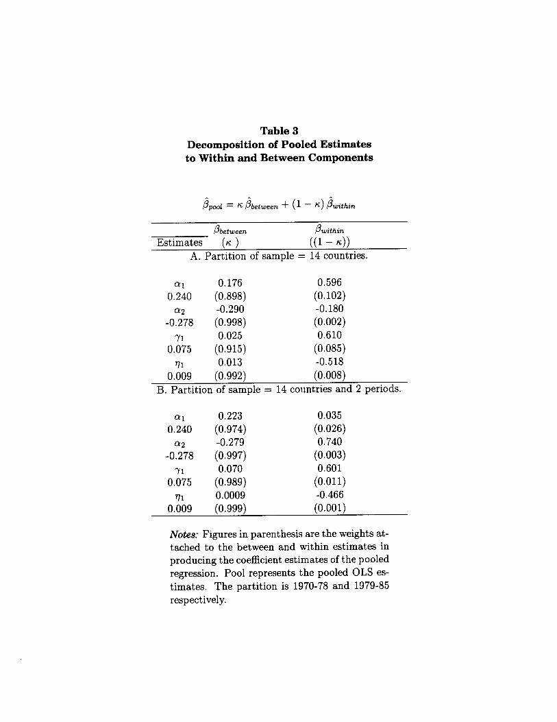
Table 3 Decomposition of Pooled Estimates to Within and Between Components

&l = K Pbetween + (1 - fi) &thin

P between Pwithin

Estimates (K ) ((1 - 4) A. Partition of sample = 14 countries.

0.20 0.176 0.596 (0.898) (0.102)

-Or;78 -0.290 -0.180 (0.998) (0.002)

o.‘,;, 0.025 0.610 (0.915) (0.085)

0.“0’09 0.013 -0.518 (0.992) (0.008)

B. Partition of sample = 14 countries and 2 periods.

Ql 0.240

-0278

o.‘,;, 71

0.009

0.223 0.035 (0.974) (0.026) -0.279 0.740 (0.997) (0.003) 0.070 0.601

(0.989) (0.011) 0.0009 -0.466 (0.999) (0.001)

Notes: Figures in parenthesis are the weights at- tached to the between and within estimates in producing the coefficient estimates of the pooled regression. Pool represents the pooled OLS estimates. The partition is 1970-78 and 1979-85 respectively.

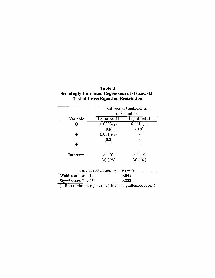
Table 4 Seemingly Unrelated Regression of (I) and (II):

Test of Cross Equation Restriction

Variable 0

a

Q

Estimated Coefficients (t-Statistic)

Equation( 1) Equation( 2) 0.030(a1) 0.03qYl)

(0.9) (0.9) O.OOl(cY~)

(0.3)

Intercept -0.001 -0.0001 (-0.025) (-0.002)

Test of restriction y1 = ~1 + a:! Wald test statistic 0.045 Significance Level* 0.832 (* Restriction is rejected with this significance level )

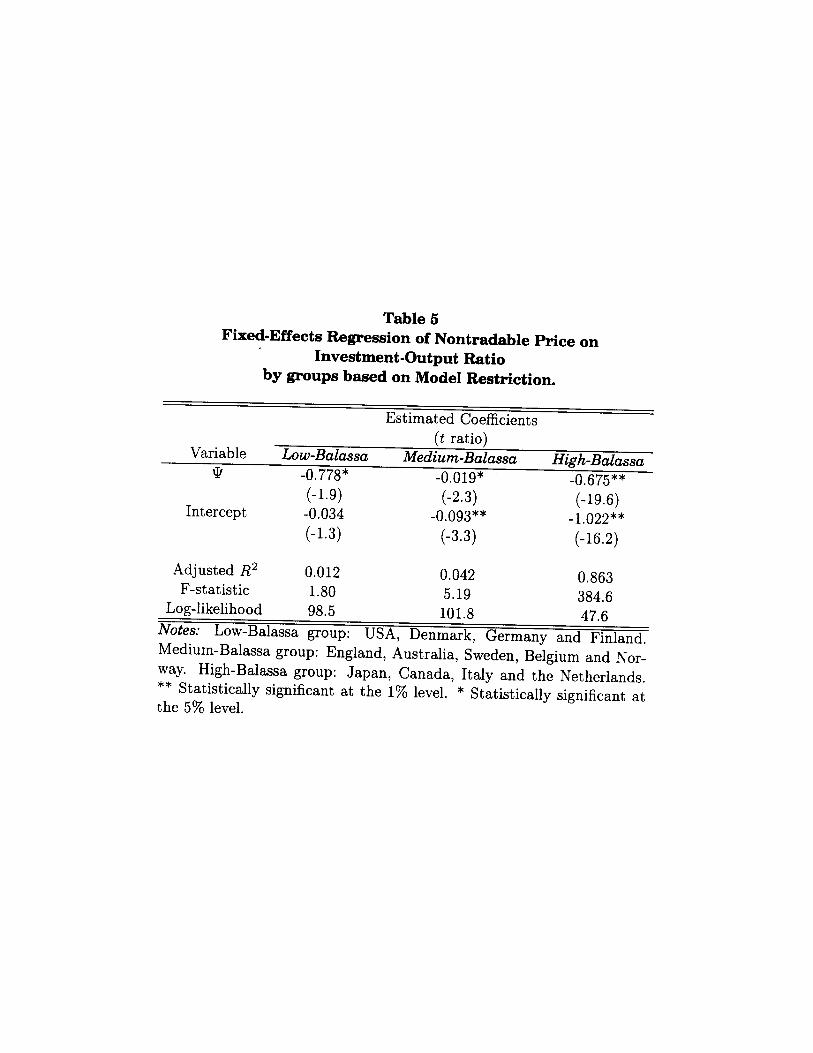
Table 5 Fixed-Effects Regression of Nontradable Price on

Investment-Output Ratio by groups based on Model Restriction.

Variable 9

Intercept

Estimated Coefficients (t ratio)

Low-Balassa Medium-Balassa High-Balassa -0.778* -0.019* -0.675** (-1.9) (-2.3) (-19.6)

-0.034 -0.093** -1.022** (-1.3) (-3.3) (-16.2)

Adjusted R2 0.012 0.042 0.863 F-statistic 1.80 5.19 384.6

Log-likelihood 98.5 101.8 47.6 Notes: Low-Balassa group: USA, Denmark, Germany and Finland. Medium-Balassa group: England, Australia, Sweden, Belgium and Nor- way. High-Balassa group: Japan, Canada, Italy and the Netherlands. ** Statistically significant at the 1% level. * Statistically significant at the 5% level.

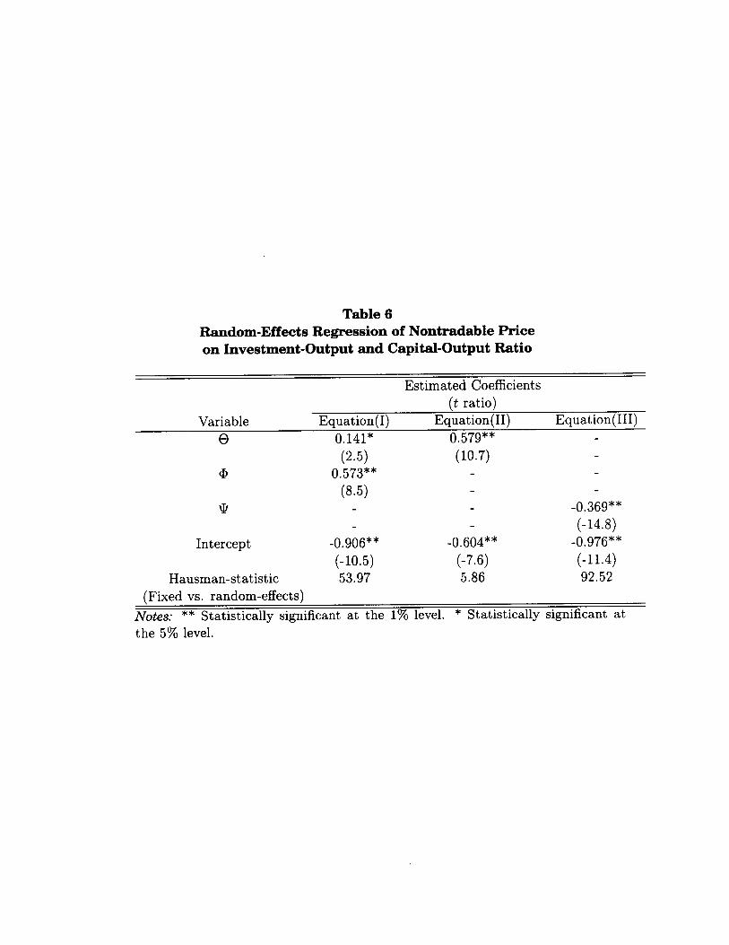
Table 6 Random-Effects Regression of Nontradable Price on Investment-Output and Capital-Output Ratio

Estimated Coefficients (t ratio)

Equation(I) Equation( II) Equation(II1) 0.141* 0.579**

Variable 8

(2.5) (10.7) @ 0.573**

(8.5) Q -0.369**

(-14.8) Intercept -0.906** -0.604** -0.976””

(-10.5) (-7.6) (-11.4) Hausman-statistic 53.97 5.86 92.52

(Fixed vs. random-effects)

Notes: ** Statistically significant at the 1% level. * Statistically significant at the 5% level.

Table 7 Comparison of Linear-Trend Filter and HP-Filter

Fixed-Effects Regression of Relative Price

Estimated Coefficients (t-ratio)

HP-Filter Linear-Trend* Variable

9 -0.518** (-17.7)

Group Dummies USA -0.88(-17.2) GER -0.99(-18.3) DEN -2.25(-17.7) FIN -1.88(-17.4) CAN -0.66(-15.7) ITY -0.85(-15.7) NLD -0.59(-8.2) JPN -0.87(-19.3) GBR -1.15(-17.9) AUS -2.25(-17.3) SWE -1.84(-18.2) BEL -2.25(-18.3) NOR -1.96(-17.6) FRA -O-91(-18.5)

Adjusted R2 F-statistic

0.945 599.7

Log-likelihood 46.38

-0.547** (-20.0)

-0.94(-19.5) -1.04(-20.8) -2.38(-20.1) -2.00(-20.0) -O-70(-17.9) -0.91(-18.6) -0.67(-10.0) -0.93(-22.6) -1.21(-20.5) -2.40(-19.7) -1.94(-20.9) -2.37(-20.1) -2.06(-20.0) -0.96(-21.4)

0.955 612.3 51.46

Notes: Linear-trend filter values are the predicted values from a regression on a constant and a linear function of time. ** Statistically significant at the 1% level.

Table 8 Pooled (Total) Regression of CPI-based Exchange Rates

on the Relative Price of Nontradables

Estimated Coefficients Variable Equation (IVa) Equation (IVb)

61 0.274 0.315 (1.25) (1.45)

60 -1.169 -1.378 (-1.15) (-1.37)

R2 0.03 0.02 Notes: p NT. HP-filtered log relative price of non- . tradables. ?jNT: Predicted value of pNT from (III). Sh? HP-filtered log real exchange rate. t ratios are in parenthesis.

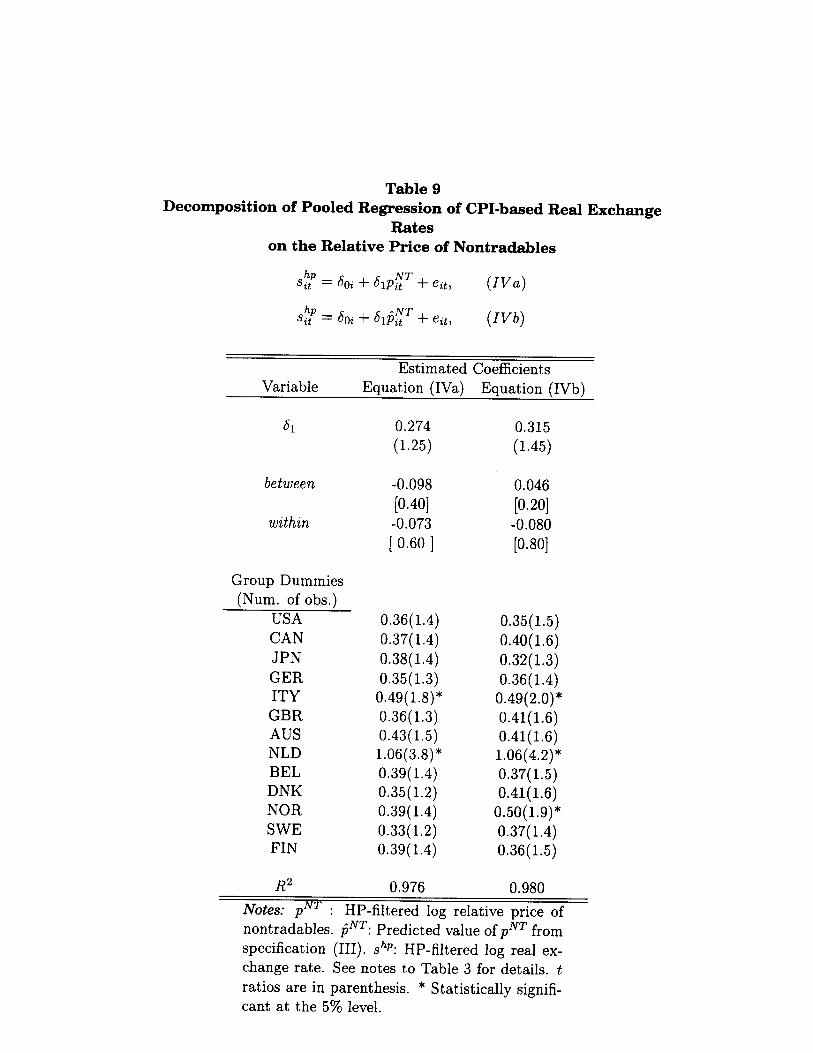
Table 9 Decomposition of Pooled Regression of CPI-based Real Exchange

Rates on the Relative Price of Nontradables

sz = 60i + 61pzT + eit, w-4

Sit hp = 6Oi + 611jgT + eit, (IVb)

Estimated Coefficients Variable Equation (IVa) Equation (IVb)

between

within

Group Dummies (Num. of obs.)

USA CAN JPN GER ITY GBR AUS NLD BEL DNK NOR SWE FIN

R2

0.274 (1.25)

-0.098 [0.40] -0.073 [ 0.60 ]

0.36(1.4) 0.37(1.4) 0.38(1.4) 0.35(1.3)

0.49( 1.8)* 0.36(1.3) 0.43(1.5) 1.06(3.8)* 0.39( 1.4) 0.35(1.2) 0.39( 1.4) 0.33(1.2) 0.39( 1.4)

0.976

0.315 (1.45)

0.046 [0.20] -0.080 [0.80]

0.35(1.5) 0.40(1.6) 0.32(1.3) 0.36(1.4)

0.49(2.0)* 0.41(1.6) 0.41(1.6) 1.06(4.2)* 0.37(1.5) 0.41(1.6)

0.50(1.9)* 0.37(1.4) 0.36(1.5)

0.980 Notes: pNT : HP-filtered log relative price of nontradables. IjNT: Predicted value of pNT from specification (III). shp: HP-filtered log real exchange rate. See notes to Table 3 for details. t ratios are in parenthesis. * Statistically significant at the 5% level.

Table 10 Pooled Regression of GDP deflator-based Real Exchange Rates

-on the Relative Price of Nontradables

Estimated Coefficients Variable Eauation (IVa) Eauation (IVb)

61 -0.921 -0.578 (-0.6) (-0.4)

60 1.475 0.954

(0.7) (04 R2 0.04 0.02

Notes: pNT : HP-filtered log relative price of nontradables. ?jNT: Predicted value of pNT from specification (III). . shP. HP-filtered log real exchange rate. t ratios are in parenthesis. * Sta- tistically significant at the 5% level. Number of observations = 112.

Table 11 Decomposition of Pooled Regression of GDP deflator-based Real

Exchange Rate on the Relative Price of Nontradables

shp zt = Soi + 6pzT + eit,

s,h;” = Soi + 61$~T + eit,

(IV4

ww

Variable Estimated Coefficients

Equation (IVa) Equation (IVb)

between

within

Group Dummies GER FRA ITY GBR NLD BEL DNK

R2

-0.921 -0.578 (-0.6) (-0.4)

-0.009 [0.44]

-1.610 [ 0.561

2.41(2.6)* 2.40(2.6)* 2.56(2.7)* 2.38(2.4)* 3.12(3.3)* 2.38(2.5)* 2.46(2.6)*

0.918

0.004 [0.30]

-0.817 [0.70]

1.19( 1.5) 1.19(1.5) 1.33(1.7) 1.19( 1.5)

1.91(2.4)* 1.17(1.5) 1.23( 1.6)

0.954

Notes: Weights, (IC), are in square brackets. See notes to Table 3 for details. pNT : HP-filtered log relative price of nontradables. IjNT: Pre- dicted value of p NT from specification (III). sh? HP-filtered log real exchange rate. t ratios are in parenthesis. * Statistically significant at the 5% level. Number of observations = 112.

Documents

The Balassa-Samuelson Model: A General Equilibrium Appraisal*