180

Reihe Ökonomie Economics Series

The Balassa-Samuelson Effect in ‘East & West’Differences and Similarities

Martin Wagner

180

Reihe Ökonomie

Economics Series

The Balassa-Samuelson Effect in ‘East & West’Differences and Similarities

Martin Wagner

November 2005

Institut für Höhere Studien (IHS), Wien Institute for Advanced Studies, Vienna

Contact: Martin Wagner Department of Economics and Finance Institute for Advanced Studies Stumpergasse 56, 1060 Vienna, Austria

: +43/1/599 91-150 fax: +43/1/599 91-163 email: Martin.Wagner@ihs.ac.at

Founded in 1963 by two prominent Austrians living in exile – the sociologist Paul F. Lazarsfeld and the economist Oskar Morgenstern – with the financial support from the Ford Foundation, the AustrianFederal Ministry of Education and the City of Vienna, the Institute for Advanced Studies (IHS) is the firstinstitution for postgraduate education and research in economics and the social sciences in Austria.The Economics Series presents research done at the Department of Economics and Finance and aims to share “work in progress” in a timely way before formal publication. As usual, authors bear fullresponsibility for the content of their contributions. Das Institut für Höhere Studien (IHS) wurde im Jahr 1963 von zwei prominenten Exilösterreichern –dem Soziologen Paul F. Lazarsfeld und dem Ökonomen Oskar Morgenstern – mit Hilfe der Ford-Stiftung, des Österreichischen Bundesministeriums für Unterricht und der Stadt Wien gegründet und istsomit die erste nachuniversitäre Lehr- und Forschungsstätte für die Sozial- und Wirtschafts-wissenschaften in Österreich. Die Reihe Ökonomie bietet Einblick in die Forschungsarbeit der Abteilung für Ökonomie und Finanzwirtschaft und verfolgt das Ziel, abteilungsinterneDiskussionsbeiträge einer breiteren fachinternen Öffentlichkeit zugänglich zu machen. Die inhaltlicheVerantwortung für die veröffentlichten Beiträge liegt bei den Autoren und Autorinnen.

Abstract

Based on two detailed Balassa-Samuelson (BS) studies, Wagner and Hlouskova (2004) for eight Central Eastern European countries (CEECs) and Wagner and Doytchinov (2004) for ten Western European countries (WECs), this study assesses the differences and similarities of the BS effect between these two country groups. The econometric results show that the BS effect may have been overestimated in previous studies due to application of inappropriate first generation panel cointegration methods. When appropriately quantified, the BS effect itself explains RER movements respectively inflation differentials only to a small extent. However, extended BS relationships that include additional variables allow for an adequate modelling of inflation. Based on the comparative analysis we draw some conclusions for monetary policy in the future enlarged Euro Area.

Keywords Balassa-Samuelson effect, Central and Eastern Europe, Western Europe, non-stationary panels, inflation simulations

JEL Classification F02, O40, O57, P21, P27

Comments Support from the Jubiläumsfonds of the Oesterreichische Nationalbank under grant Nr. 9557 is gratefully acknowledged. Part of this work has been done whilst visiting the Economics Department ofthe European University Institute, whose hospitality is gratefully acknowledged. I thank JaroslavaHlouskova, Robert Kunst, Karlhans Sauernheimer, and conference participants at the meeting of theChristian-August-Gesellschaft in Sulzbach-Rosenberg, in particular my discussant Franco Reither, forhelpful comments. The usual disclaimer applies.

Contents

1 Introduction 1

2 The Balassa-Samuelson Effect 3

3 The Econometric Problems 8

4 Findings for the CEEC8 and the WEC10 10

5 Summary and Policy Implications 18

References 19

1 Introduction

Recent years have seen an enormously growing empirical literature trying to assess the

Balassa-Samuelson (BS) effect.1 The BS effect explains real exchange rate (RER) appre-

ciation (depreciation) of the home country with respect to the foreign country due to a higher

(lower) inter-sectoral productivity differential between the tradables and non-tradables sector

at home than in the foreign country (see Section 2 for a brief exposition). In this paper we use

the BS model to explain price movement respectively inflation differentials across countries,

which is an immediate consequence of the model after some minor algebraic modifications

(compare equations (3) and (4) below).

In its core version the BS model is a pure supply side explanation of RER and price move-

ments. However, in our empirical applications extended relationships that allow in particular

to also model demand side effects will be estimated to appropriately model the RER and price

behavior. Two types of additional variables are included: First, variables that are directly

related to the non-validity of certain assumptions of the basic model (like purchasing power

parity in tradables and inter-sectoral wage homogeneity) and second, demand side variables

that are incorporated in extended versions of the model (for the inclusion of per capita GDP,

see Bergstrand, 1991). Both types of variables are found to be important.

Especially for Central and Eastern European countries (CEECs), but also for Western

European Countries (WECs) numerous studies have been produced. However, it appears that

no studies comparing the findings for CEECs and WECs in order to assess the similarities

respectively dissimilarities in the real exchange rate and inflation behavior and the main

explanatory factors across these two groups of countries exist. Based on two recent detailed

studies, Wagner and Hlouskova (2004) for the CEECs and Wagner and Doytchinov (2004) for

the WECs, this paper tries to fill this gap.

Wagner and Hlouskova (2004) contains a detailed analysis of the BS effect for a sample

of eight CEECs (labelled as CEEC8) that have joined the EU on May 1, 2004: the Czech

Republic (CZE), Estonia (EST), Hungary (HUN), Latvia (LVA), Lithuania (LTU), Poland

(POL), the Slovak Republic (SVK) and Slovenia (SVN) over the period 1993–2001. The

‘foreign’ country in this panel study is given by the aggregate of eleven Western European1See e.g. the references in Wagner and Hlouskova (2004) and Wagner and Doytchinov (2004). These two

detailed studies form the basis for the investigations presented in this paper. All details concerning the dataand their sources, the aggregation procedures, the applied econometric methodologies and bootstrap algorithmsare contained in these papers and omitted here for brevity.

1

‘old’ EU member states, the WEC11. These are Austria (AUT), Belgium (BEL), Denmark

(DNK), Finland (FIN), France (FRA), Germany (GER), Great Britain (GBR), Italy (ITA),

the Netherlands (NLD), Spain (ESP) and Sweden (SWE). Thus, of the EU15 countries Greece,

Ireland, Luxembourg and Portugal are excluded because of data availability problems. This

choice of ‘foreign country’ is motivated by the fact that the Western European EU member

states are the main trading partners as well as the major source of foreign direct investment

of the CEECs. The next major integration step will be the introduction of the Euro in the

CEECs, which makes an understanding of the inflation perspectives of these countries a highly

relevant policy issue.

Wagner and Doytchinov (2004) use the WEC11 data to construct a panel of ten countries

with Germany (GER) as foreign country. We refer to this group as the WEC10. It is quite

common in the BS literature to take Germany as the foreign country, when studying Western

European economies, see e.g. Alberola and Tyrvainen (1999) or Sinn and Reutter (2001). This

is a rather natural choice given that Germany and the Deutsche Mark were the European

‘anchor’ country respectively currency before the introduction of the Euro.2 The data span

for that study is 1991–2001. The choice of Germany as foreign country may, however, be

problematic due to German reunification in October 1990. This may imply on the one hand

data quality problems and on the other hand it may also imply that Germany is a bad

‘benchmark’ for BS analysis due to the sizeable structural changes arising after reunification.

A detailed study of these issues, which are ignored in the literature, is unfortunately also

beyond the scope of this paper. From the large sets of results of those two papers we here

focus only on the mean inflation scenarios, obtained from averaging the results concerning

inflation across large numbers of econometrically well specified equations.3

In Section 2 we provide a very brief description of the basic model and the extensions

necessary for successful empirical implementation. In this section we also discuss some details

concerning the construction of the two sectors on which the model rests: the tradables and

the non-tradables sectors. In Section 3 we discuss several important econometric problems

that plague a large part of the empirical BS literature that often – as we do – performs

the empirical analysis on panels. Nonstationarity combined with cross–sectional dependence2Note, e.g. that in 2003 Germany’s share in WEC11 GDP amounted to about 24%. An open issue left for

future research is a combined study using both CEECs and WECs together in the econometric analysis. Suchan analysis will have to take into account the structural differences across the CEECs and the WECs.

3Furthermore, for brevity we only focus on the inflation scenarios generated from the extended BS equationsand will not discuss the Baumol-Bowen (BB) estimation and simulation results.

2

renders the applied so called ‘first generation’ panel unit root and panel cointegration methods

inappropriate, since those methods are all designed for cross–sectionally independent panels.

The two studies underlying the present paper show that the application of such first generation

methods results in substantial biases. Since the emergence of these substantial biases is an

important observation that is relevant for the BS literature in general, we quantify the biases

in Section 4. In Section 4 we also summarize some of the main findings concerning inflation

simulations based on well specified equations for both country groups. Finally, in Section 5

we briefly summarize and discuss some policy implications.

2 The Balassa-Samuelson Effect

Balassa (1964) and Samuelson (1964) present models in which different productivity growth

differentials between the tradables and non-tradables goods sectors across countries are an

important factor in explaining real exchange rate movements, respectively differences in the

evolution of national price levels.4

The model is formulated in terms of a two-sector small open economy (SOE). The two

sectors are the tradables sector (superscript T ) and the non-tradables sector (superscript N).

Being a SOE the home country takes the world interest rate and the price of tradables (P T )

as given and hence only the price of non-tradables (PN ) and the wages (W T , WN ) are set

within the country. Denote with prel = pN − pT , the logarithm of the relative price of non-

tradables to tradables (throughout the paper we use lower case letters to indicate logarithms).

Production in both sectors takes place within perfectly competitive firms that use labor and

capital as inputs and a key assumption of the model is that the productivities in both sectors

differ (with in general higher productivity (growth) in the tradables sector).

Assume for the moment further that labor is perfectly mobile across sectors, which implies

wage homogeneity, i.e. wT = wN . Now, assume that productivity growth is higher in the

tradables sector than in the non-tradables sector, i.e. ∆aT > ∆aN (with ai denoting the

logarithm of total factor productivity in sector i = T, N and with ∆ the first difference

operator). Increasing productivity implies that wages grow at the corresponding rate in the

tradables sector (with the price of the tradable good determined on the world market). Under4Ghironi and Melitz (2005) present a stochastic general equilibrium model with heterogeneous firms that

leads to BS type effects. An earlier general equilibrium analysis of the BS model is given by Asea and Mendoza(1994). Aukrust (1977) presents a model very similar to the BS model, with a sheltered and a non-shelteredsector. Bhagwati (1980) presents a model in which real exchange rate movements are driven by scarcity ofcapital and hence low productivity in developing countries.

3

the just made assumption of perfect labor mobility wages have to grow at the same rate in

the non-tradables sector in order to attract labor. Since productivity grows slower in the

non-tradables sector than in the tradables sector, the non-tradables sector has to increase its

prices to stay profitable. Thus, the relative price prel increases. The described domestic effect

is the so called Baumol-Bowen effect, first described in Baumol and Bowen (1966). It can be

formalized most easily when resorting to sectoral Cobb-Douglas production functions, which

result (by appropriately combining the first order conditions for profit maximization) in

prel = c +αN

αTaT − aN , (1)

where αi denotes the factor share of labor in sector i and c is a constant depending upon the

exogenous interest rate and the factor shares.5 Empirically, wage homogeneity is rejected and

the equation corresponding to (1) without the wage homogeneity assumption is given by:6

prel = c +αN

αTaT − aN + αN (wN − wT ) (2)

Thus, the increase of relative prices outlined above is mitigated by lower wage growth in the

non-tradables sector when labor is not perfectly mobile across sectors.

Combining the above effect for two countries by using the definition of the real exchange

rate then leads to the Balassa-Samuelson effect. Denote the logarithm of the real exchange

rate by q = e+p∗−p, where e denotes the logarithm of the nominal exchange rate and p∗ and

p are the logarithms of the price levels abroad and at home.7 The aggregate price levels are

given by weighted averages of the sectoral price levels, i.e. p = (1− δ)pT + δpN and similarly

for p∗.

Using the definitions of the RER and the prices yields, by inserting (2) for both countries,

after some rearrangements

q = c + qT − δ

(αN

αTaT − aN + αN (wN − wT )

)+ δ∗

(αN∗

αT∗ aT∗ − aN∗ + αN∗(wN∗ − wT∗))

, (3)

with qT = e+ pT∗− pT denoting the real exchange rate of tradables. It is commonly assumed

in the literature that purchasing power parity (PPP) holds in tradables, which consequently

implies in its ‘strong’ formulation that qT = 0. Empirically, the real exchange rate in trad-

ables is found to be non-stationary for both country groups, for the CEEC8 vis-a-vis the5The letter c is throughout used to denote constants in the equations, generally not the same across

equations.6Due to unit root nonstationary behavior of sectoral wages, wage homogeneity is empirically defined as

cointegration between wT and wN . Cointegration between sectoral wages is rejected throughout.7Throughout the paper the superscript ∗ indicates variables of the foreign country.

4

WEC11 and for the WEC10 vis-a-vis Germany. Thus, compared to many studies our em-

pirical investigations focus on the extended BS effect as illustrated in equation (3), where in

addition to the productivity differential also sectoral wage differentials and deviations from

PPP in tradables are contained as explanatory variables.

The above equation (3) explains RER movements (by taking the first difference of the

equation) as due to differential inter-sectoral productivity growth differentials across coun-

tries (abstracting for simplicity from the wage terms and deviations from PPP in tradables).

The widespread observation of larger productivity differentials in developing or catching-up

economies, due to especially large productivity growth in tradables, has thus made the BS

model a valuable tool for explaining RER appreciations (∆q < 0) of such countries vis-a-vis

advanced countries. Some relatively early empirical contributions include Canzoneri, Cumby

and Diba (1999) or DeGregorio and Wolf (1994).

Note that by rearranging (3) further, one obtains an equation that allows to explain price

differentials (or after taking differences inflation differentials) across countries, which is of

particular importance in the context of European monetary unification. Note in particular

that in this equation then the nominal exchange rate drops out.

p − p∗ = c + pT − pT∗ + δ(

αN

αT aT − aN + αN (wN − wT ))−

δ∗(

αN∗αT∗ aT∗ − aN∗ + αN∗(wN∗ − wT∗)

) (4)

When moving from the theoretical model to the empirical implementation several deci-

sions concerning the data have to be made, most notably the sectoral classification. As the

tradables sector we define the aggregate over NACE8 sectors C (mining and quarrying), D

(manufacturing) and E (electricity, gas and water supply). The non-tradables sector is given

by sectors F (construction) to K (real estate and business activities). Sectors A (agriculture)

and B (fishing) are aggregated to agriculture and sectors L (public administration and de-

fence) to P (private households with employed persons) are aggregated to the public sector.

These two additional sectors are not included in the econometric analysis, but have to be

taken into account when performing inflation simulations. With the chosen classification the

tradables and non-tradables sectors together comprise, depending upon country, about 75 to

80% of GDP.

Concerning the choice of dependent variables, for both the real exchange rate (see 3) and

the price differential (see 4), we discuss narrow and wide specifications. The narrow measures8NACE is the (french) acronym for Classification of Economic Activities in the European Community.

5

Name BS variable(s) Separate wagesA δit(arel

it + αNit wrel

it ) − δ∗t (arel∗t + αN

t∗wrel∗t ) −−

B (arelit + αN

it wrelit ) − (arel∗

t + αNt∗wrel∗

t ) −−C δita

relit − δ∗t arel∗

t wrelBS,it

D arelit − arel∗

t wrelBS,it

E arelit , arel∗

t wrelBS,it

Table 1: Choices concerning the BS variables used for the econometric analysis, see theexplanations in the text.

are based on only the RERs respectively price differentials of the tradables and non-tradables

sectors (e.g. pT+N − pT+N∗). The wide measures are based on the GDP deflators for the

CEEC8 and the Harmonized Index of Consumer Prices (HICP) for the WEC10. These two

measures are not directly in line with the theoretical model, but are ultimately the relevant

quantities when studying inflation and real exchange rate dynamics.9 Using both types of

measures allows to see whether there are systematic differences in the results obtained from

the narrow and the wide measures.

The final decision that has to be made is the empirical specification of the BS variable.

In this respect we propose five choices, summarized in Table 1. Variable A, with wrel =

wN −wT , corresponds most closely to the variables appearing in the theoretical relationships

(compare (3) and (4)), only the ratio αN

αT is omitted. This is done because preliminary analysis

with variables including this ratio led to unsatisfactory econometric results. Neglecting the

differences in sectoral composition across countries, i.e. neglecting δit and δ∗t defines variable

B. In variables C to E the wage term is taken out of the BS variable and considered separately

via wrelBS,it = wrel

it − wrel∗t . The difference between C and D is again the neglect of δit and

δ∗t . In variable E finally the productivity at home and in the foreign country enter the

equations separately. Obviously, E nests D and the corresponding restriction of coefficients

of equal magnitude and opposite sign can be tested. The restriction is in most cases not

rejected, and thus in the final specifications mainly the variable D is used and only in a few

equations E remains as explanatory variable. Also in the literature D appears to be the

most commonly used variable. Using several BS variables allows to study the robustness9Also, Harberger (2004) argues for the use of wide real exchange rate measures. Note additionally that for

the WEC10 the correlation between the inflation rate based on the GDP deflators and the HICPs is above 0.9for all countries. For the CEEC8 no HICP series are available as of now, therefore we use the GDP deflatorseries. Details concerning the data, their construction and their sources are contained in the underlyingcompanion papers, as mentioned before.

6

0

2

4

6

8

10

12

-2 -1 0 1 2 3 4 5

d(arel)-d(arel*)

d(p

T+

N)-

d(p

T+

N* )

CZE

SVK

LVALTU

ESTPOL

HUN

SVN

-1

0

1

2

3

-1 0 1 2 3 4

d(arel)-d(arel*)

d(p

rel )-d

(pre

l*)

ESP

GBR

ITA

DNK

NLD

AUT

BEL FRA

FIN

SWE

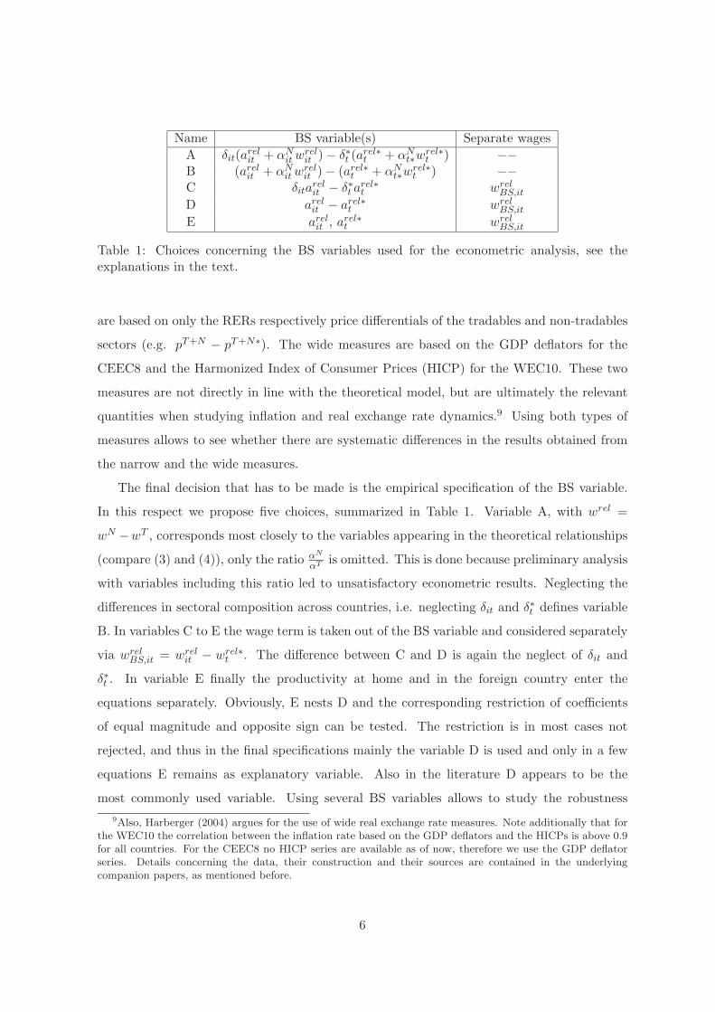
Figure 1: Unconditional correlation between inter-sectoral productivity growth differential,∆arel − ∆arel∗, and price differential between home and foreign country. The left graphdisplays the correlation between the CEEC8 and the WEC11 with ∆pT+N − ∆pT+N∗ asprice differential measure, averaged over the period 1996–2001. The right graph displaysthe correlation between the WEC10 and Germany with ∆prel − ∆prel∗ as price differentialmeasure, averaged over the period 1992–2001.

respectively sensitivity of the BS effect with respect to the specification of the BS variable.

In Figure 1 we display the (unconditional) correlation between the price differential be-

tween the home and the foreign country and the inter-sectoral productivity growth differential

between the home and the foreign country. In the left picture, for the CEEC8, we use the

differential of the inflation rates of T and N only, i.e. ∆pT+N − ∆pT+N∗, with the WEC11

as the foreign country. In the right picture for the WEC10 we use the differential of relative

price inflation, i.e. ∆prel − ∆prel∗, with Germany as the foreign country. According to the

BS model both measures should be positively correlated with the inter-sectoral productivity

growth differential between home and foreign country. This is confirmed in the graphs. It

furthermore holds true in all countries that productivity growth is higher in tradables than in

non-tradables, whereas prices grow faster in non-tradables than in tradables.10 Note for later

reference the differences in the vertical scale of the two graphs, from 0 to 12% for the CEEC8

and from -1 to 3% for the WEC10. This, of course, reflects the fact that the CEECs are

still at a higher level of inflation than the WECs. The exploratory, graphical analysis gives

sufficient support to turn to an econometric analysis. We start with a discussion of problems

arising when doing so in the following section.10The only exception is Denmark, where prices of tradables grow slightly faster than non-tradables prices

over the sample period.

7

3 The Econometric Problems

The short time span of available annual sectoral data series necessitates the application of

panel methods.11 Given the nonstationary character of many economic time series conse-

quently panel unit root and panel cointegration methods are often applied, e.g. Egert (2002)

or Egert et al. (2003). However, the nonstationary panel methods applied so far in the BS

literature are so called first generation methods, which are based on the assumption of cross-

sectional independence. For almost all panels of economic time series this assumption is

violated. For a detailed analysis of this problem in real exchange rate panels, see Wagner

(2005), who shows that not accounting for the cross-sectional dependence that is present

almost by construction for real exchange rates can fundamentally alter the conclusions con-

cerning stationarity or unit root nonstationarity. The short time span (more than the small

cross-sectional dimension) poses another problem for the methods usually applied. Being

rather straightforward extensions of time series methods implies that for panels with short

time dimensions such methods perform rather poor, since they ‘inherit’ the poor small sam-

ple performance of time series unit root and cointegration tests, see Hlouskova and Wagner

(2005) for ample simulation evidence.

These two problems together lead us to consider bootstrap inference in order to improve

both the small sample performance and to allow for a certain degree of cross-sectional de-

pendence. This has substantial impact on the results, see Figure 2. The figure displays the

asymptotic distribution (which is the standard normal distribution) and the bootstrap test

distributions for five asymptotically standard normally distributed panel unit root tests for

the relative prices prel for the WEC10.12 The five panel unit root tests applied are devel-

oped in Levin, Lin and Chu (2002) (LL), Breitung (2000) (UB), Im, Pesaran and Shin (2003)

(IPS), Harris and Tzavalis (1999) (HT) and Im, Pesaran and Shin (1997) (IPS-LM). A clear

observation emerges: All tests’ bootstrap distributions are far off the asymptotic distribution.

This implies that inference based on asymptotic critical values will be highly misleading, since

the actual size can be arbitrarily far away from the nominal size.

Similar results are obtained for all variables and thus we obtain, when resorting to boot-

strap methods, quite different conclusions than when resorting to inference based on the11Some authors use time series methods and quarterly data, e.g. Alberola and Tyrvainen (1999) for WECs

or Egert (2002) (who uses both time series and first generation panel cointegration tests) for CEECs.12Similar pictures are available for the CEEC8 and for the other variables.

8

−10 −8 −6 −4 −2 0 2 4 6 8 100

0.1

0.2

0.3

0.4

0.5

LLUBIPSHTIPS−LMN (0,1)

Figure 2: Bootstrap test statistic distributions for relative prices, prel, for the five asymptot-ically standard normally distributed panel unit root tests. The figure displays the results forthe WEC10.The results are based on the non-parametric bootstrap with 5000 replications. Fixed effectsare included.

asymptotic critical values.13 Concerning the unit root test results we find quite some evi-

dence for unit root nonstationarity, also when resorting to bootstrap inference. With unit

root nonstationary variables the possibility of cointegration arises in equations of the form (3)

or (4). Thus, the whole array of equations with both the RER differentials and the price dif-

ferentials as dependent variable as well as the different choices for the BS variable are tested

for cointegration. The results are very clear: When resorting to bootstrap inference no sup-

port for cointegration remains, whereas inference based on the asymptotic critical values leads

to quite some evidence for cointegration. These findings have the strong implication that BS

studies based on panel cointegration analysis may be substantially biased, since in the absence

of cointegration the applied estimators are of course inconsistent. To quantify the potential

biases we perform estimation (including specification analysis) using both panel cointegration

estimators and estimation in growth rates and use the differences in results as our measure

of the bias introduced by inappropriately resorting to first generation panel cointegration

estimation techniques.

Resorting to estimation in growth rates has two further important advantages over (inap-

propriate) first generation panel cointegration estimation. First, it allows to include additional

explanatory variables more easily. The first generation panel cointegration estimators a la13The implemented bootstrap methods (parametric, non-parametric and RBB) are described in detail in

Appendix C of Wagner and Hlouskova (2004).

9

Mark and Sul (2003) or Pedroni (2000) require that all regressors are integrated of order one,

but not cointegrated amongst themselves. Thus, additional cointegrating relationships as well

as the inclusion of e.g. stationary regressors are excluded. This, of course, restricts applica-

bility, especially in situations with a large number of potential explanatory variables. Second,

the regressors are assumed to be exogenous in first generation panel cointegration estimation.

This assumption is not necessary when estimating in growth rates. Even more, exogeneity

testing can be performed and if necessary instrumental variable estimation is available as

well.14 These additional issues make the quantification of the ‘cointegration bias’ even more

relevant.

4 Findings for the CEEC8 and the WEC10

For both country groups a large number of equations is estimated. We consider five BS vari-

ables, four dependent variables and in addition error correction formulations (i.e. equations

in growth rates where the lagged cointegrating relationship is added as regressor). The speci-

fication analysis starts from considering lags up to one and as additional explanatory demand

side variables per capita GDP growth, total consumption growth and investment growth. For

the WEC10 only total consumption growth is significant. Investment as demand side variable

(following Fischer, 2004) appears to be insignificant throughout. For the equations in growth

rates we test for exogeneity of the regressors by applying the Durbin-Wu-Hausman test. The

null hypothesis of regressor exogeneity is only rejected in a few cases, in which we resort to

instrumental variable estimation.

Following the estimation strategy outlined above Wagner and Hlouskova (2004) find fifteen

equations where all coefficients signs are according to theory for the CEEC8. For the WEC10

fourteen well-specified equations with correct coefficient signs are presented in Wagner and

Doytchinov (2004). Note again that the core estimation results are derived when estimating

in growth rates. Panel cointegration and error correction estimations are only performed to

assess the bias this introduces.

The quantified BS effect, measured as contribution to the inflation differential, and the

associated cointegration biases are displayed in detail in Tables 2 and 3. Throughout, the

BS effect is defined as the coefficient corresponding to the BS variable times the average of14Furthermore it is an advantage that all the usual panel techniques to handle cross-sectional dependence

and/or heteroskedasticity are available for GLS/IV estimation in growth rates.

10

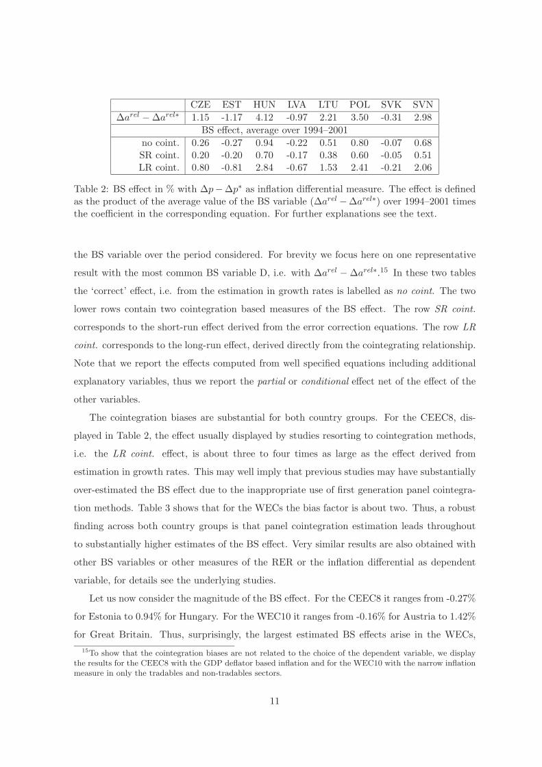
CZE EST HUN LVA LTU POL SVK SVN∆arel − ∆arel∗ 1.15 -1.17 4.12 -0.97 2.21 3.50 -0.31 2.98

BS effect, average over 1994–2001no coint. 0.26 -0.27 0.94 -0.22 0.51 0.80 -0.07 0.68SR coint. 0.20 -0.20 0.70 -0.17 0.38 0.60 -0.05 0.51LR coint. 0.80 -0.81 2.84 -0.67 1.53 2.41 -0.21 2.06

Table 2: BS effect in % with ∆p−∆p∗ as inflation differential measure. The effect is definedas the product of the average value of the BS variable (∆arel −∆arel∗) over 1994–2001 timesthe coefficient in the corresponding equation. For further explanations see the text.

the BS variable over the period considered. For brevity we focus here on one representative

result with the most common BS variable D, i.e. with ∆arel − ∆arel∗.15 In these two tables

the ‘correct’ effect, i.e. from the estimation in growth rates is labelled as no coint. The two

lower rows contain two cointegration based measures of the BS effect. The row SR coint.

corresponds to the short-run effect derived from the error correction equations. The row LR

coint. corresponds to the long-run effect, derived directly from the cointegrating relationship.

Note that we report the effects computed from well specified equations including additional

explanatory variables, thus we report the partial or conditional effect net of the effect of the

other variables.

The cointegration biases are substantial for both country groups. For the CEEC8, dis-

played in Table 2, the effect usually displayed by studies resorting to cointegration methods,

i.e. the LR coint. effect, is about three to four times as large as the effect derived from

estimation in growth rates. This may well imply that previous studies may have substantially

over-estimated the BS effect due to the inappropriate use of first generation panel cointegra-

tion methods. Table 3 shows that for the WECs the bias factor is about two. Thus, a robust

finding across both country groups is that panel cointegration estimation leads throughout

to substantially higher estimates of the BS effect. Very similar results are also obtained with

other BS variables or other measures of the RER or the inflation differential as dependent

variable, for details see the underlying studies.

Let us now consider the magnitude of the BS effect. For the CEEC8 it ranges from -0.27%

for Estonia to 0.94% for Hungary. For the WEC10 it ranges from -0.16% for Austria to 1.42%

for Great Britain. Thus, surprisingly, the largest estimated BS effects arise in the WECs,15To show that the cointegration biases are not related to the choice of the dependent variable, we display

the results for the CEEC8 with the GDP deflator based inflation and for the WEC10 with the narrow inflationmeasure in only the tradables and non-tradables sectors.

11

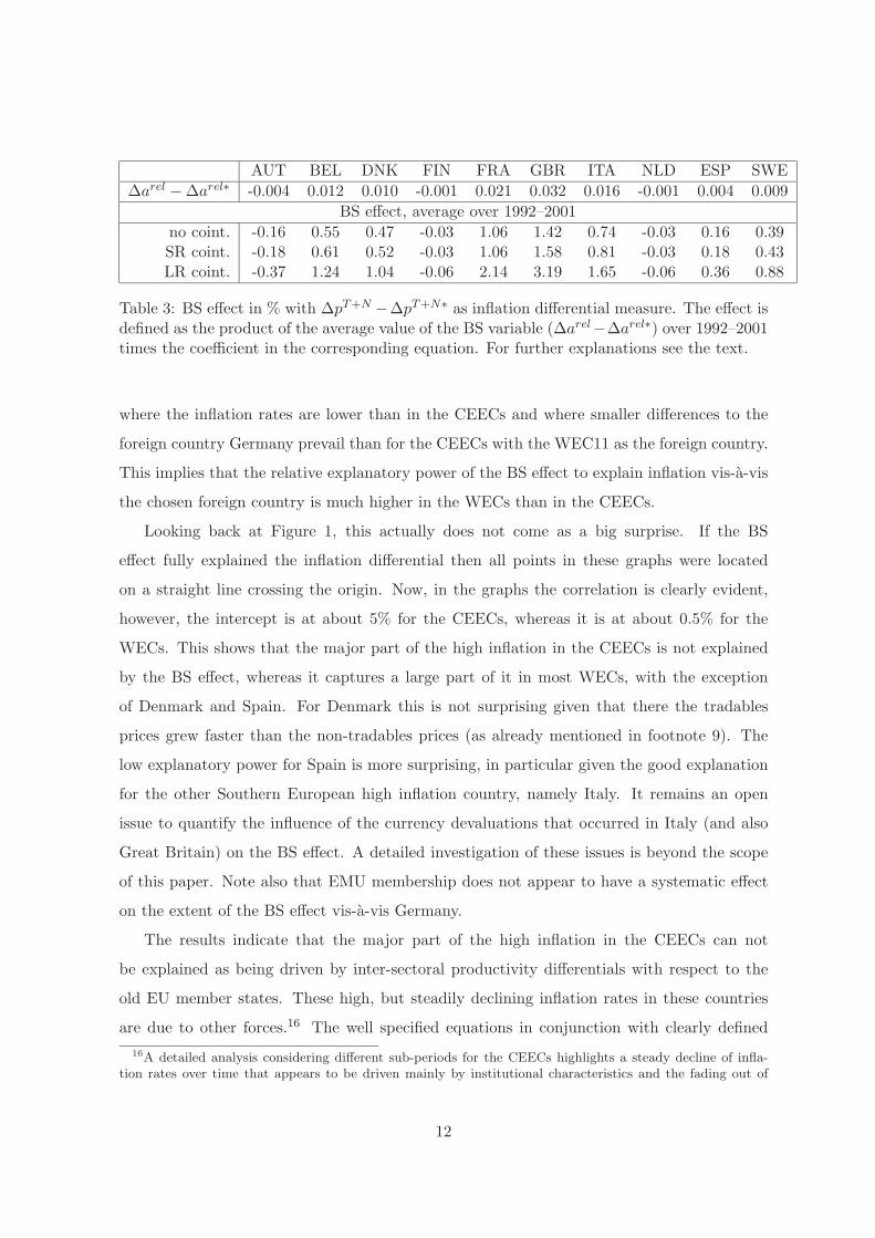
AUT BEL DNK FIN FRA GBR ITA NLD ESP SWE∆arel − ∆arel∗ -0.004 0.012 0.010 -0.001 0.021 0.032 0.016 -0.001 0.004 0.009

BS effect, average over 1992–2001no coint. -0.16 0.55 0.47 -0.03 1.06 1.42 0.74 -0.03 0.16 0.39SR coint. -0.18 0.61 0.52 -0.03 1.06 1.58 0.81 -0.03 0.18 0.43LR coint. -0.37 1.24 1.04 -0.06 2.14 3.19 1.65 -0.06 0.36 0.88

Table 3: BS effect in % with ∆pT+N −∆pT+N∗ as inflation differential measure. The effect isdefined as the product of the average value of the BS variable (∆arel−∆arel∗) over 1992–2001times the coefficient in the corresponding equation. For further explanations see the text.

where the inflation rates are lower than in the CEECs and where smaller differences to the

foreign country Germany prevail than for the CEECs with the WEC11 as the foreign country.

This implies that the relative explanatory power of the BS effect to explain inflation vis-a-vis

the chosen foreign country is much higher in the WECs than in the CEECs.

Looking back at Figure 1, this actually does not come as a big surprise. If the BS

effect fully explained the inflation differential then all points in these graphs were located

on a straight line crossing the origin. Now, in the graphs the correlation is clearly evident,

however, the intercept is at about 5% for the CEECs, whereas it is at about 0.5% for the

WECs. This shows that the major part of the high inflation in the CEECs is not explained

by the BS effect, whereas it captures a large part of it in most WECs, with the exception

of Denmark and Spain. For Denmark this is not surprising given that there the tradables

prices grew faster than the non-tradables prices (as already mentioned in footnote 9). The

low explanatory power for Spain is more surprising, in particular given the good explanation

for the other Southern European high inflation country, namely Italy. It remains an open

issue to quantify the influence of the currency devaluations that occurred in Italy (and also

Great Britain) on the BS effect. A detailed investigation of these issues is beyond the scope

of this paper. Note also that EMU membership does not appear to have a systematic effect

on the extent of the BS effect vis-a-vis Germany.

The results indicate that the major part of the high inflation in the CEECs can not

be explained as being driven by inter-sectoral productivity differentials with respect to the

old EU member states. These high, but steadily declining inflation rates in these countries

are due to other forces.16 The well specified equations in conjunction with clearly defined16A detailed analysis considering different sub-periods for the CEECs highlights a steady decline of infla-

tion rates over time that appears to be driven mainly by institutional characteristics and the fading out of

12

inflation scenarios discussed below will show, however, that an extended BS framework that

takes into account also demand side characteristics as well as the developments in the public

sector and in agriculture leads to a very good description of the inflation process. Thus,

the low explanatory power does not dismiss the BS model, but highlights the importance

of going beyond the basic pure supply side version and to consider well specified extended

relationships.

To assess the explanatory (respectively predictive) power of the well specified models

developed by augmenting the BS model with additional variables, e.g. relative tradables

prices, inter-sectoral wage differentials and demand side variables, we consider now the results

of inflation simulations.

These are only done for all well specified equations in growth rates, given the large cointe-

gration biases found above. We perform inflation simulations for all four dependent variables

(narrow and wide; real exchange rate and price differential), to see whether systematic dif-

ferences emerge. Doing so requires to choose values for the explanatory variables included.

First and foremost it requires to specify the inflation rate in the foreign country, where we

choose 2% for both the WEC11 and also for Germany. This corresponds to the 2% inflation

target of the European Central Bank and corresponds also very closely to the actual average

HICP inflation for Germany of 2.09% over the sample period. Furthermore, we report here

results assuming that tradables prices move similarly across all countries, i.e. ∆pT = ∆pT∗.17

For the equations with the narrow measures as dependent variables we also need to specify

the inflation behavior in agriculture and the public sector. The base-line case considered here

is to set their values equal to the historical averages, where we consider two sub-periods for

the CEEC8 to allow for disinflation. The first one is 1994–2001 and the second is 2000–2001,

i.e. the end of the sample only. Finally, for the equations with the real exchange rates as

dependent variable an assumption concerning the evolution of the nominal exchange rate to

the Euro has to be made. We assume that this exchange rate is constant for all countries.

Obviously, for the Euro Area countries this is fulfilled by construction. For some of the

other countries the nominal exchange fluctuates very little and for some of these countries

the conversion rates for the introduction of the Euro have already been announced. Thus,

inflationary shocks due to the transition process (e.g. price liberalization steps).17Results obtained by replacing this assumption by the actual movements are contained in Wagner and

Doytchinov (2004) and Wagner and Hlouskova (2004). For the WEC10 the results only differ significantly forSweden across these two simulation experiments.

13

in particular in a forward looking perspective the assumption of a constant Euro exchange

rate appears a plausible choice.18 For the additional demand variables, real per capita GDP

growth and real total consumption growth, we choose the values as follows. For the CEEC8

we use the mean values of the convergence scenarios of Wagner and Hlouskova (2005), who

present a detailed analysis of the real convergence prospects of ten CEECs. For the WEC10,

where only total consumption appears significant, we resort to the forecasts published in

OECD (2004). We next briefly discuss the results for both country groups and afterwards we

turn to a comparison of the findings.

The results for the CEEC8 are displayed in Table 4. The upper panel shows the results

when the averaging period for the variables is 1994–2001 and the lower one with the averages

only over 2000–2001. In the table we display the mean, minimum, maximum and standard

deviation across all equations and furthermore the means only over the equations with the

widely defined dependent variables and those with the narrowly defined dependent variables.

The difference between the two stems from the fact that for the equations with the narrowly

defined dependent variable the inflation contribution from the agricultural and public sectors

is added separately, whereas it is implicitly included in the regressions where the widely

defined variables are used as dependent variables. For the CEEC8 countries this leads to

substantial differences, with the mean over the wide equations only equal to 4.73% and the

mean over the narrow equations only equal to 6.24% (when looking at the group in total).

Thus, the narrow equations lead to on average higher (to high) inflation simulations and the

wide equations lead to on average lower (too low) inflation. Both of our approaches do not

model the inflation dynamics in agriculture and the public sector and thus in particular do

not investigate the relationships between the inflation rates across sectors. Our results show

that the two approaches span the range of potential outcomes in this respect. Note that for

the WEC10 no such differences occur and thus for these countries we do not display the means

over the sub-groups of equations separately. For the CEECs our results indicate a potential

payoff for detailed investigations of the inflationary dynamics in agriculture and the public

sectors, this is beyond the scope of this study and in fact of the BS literature in general.

Comparing the upper and the lower panel of Table 4 (and for brevity only the mean) we

see that the inflation scenarios track the disinflation process observed since the mid 1990s18Of course, for some countries like Great Britain, the assumption of a constant exchange rate is only

motivated by non-predictability of exchange rates arguments.

14

CZE EST HUN LVA LTU POL SVK SVN CEEC81994–2001

Min 2.89 3.20 3.52 2.71 3.33 3.99 2.78 2.52 3.83Max 6.63 8.73 7.66 10.31 10.98 10.13 5.21 6.67 7.84

Mean 4.60 6.00 5.44 6.64 6.90 7.16 3.84 4.49 5.99Std. Dev. 0.92 1.67 1.58 2.36 2.59 2.05 0.80 1.34 1.30Meanwide 4.36 4.89 4.24 6.47 6.47 5.92 3.52 3.51 5.05

Meannarrow 4.87 7.27 6.81 6.83 7.39 8.58 4.20 5.61 7.06Actual ∆p 7.21 14.53 14.51 10.94 15.87 14.37 6.98 10.30 12.25

2000–2001Min 2.14 1.52 3.36 1.48 -1.70 3.08 1.64 1.15 3.10Max 5.73 6.84 7.06 10.58 10.13 9.60 4.63 6.00 7.23

Mean 4.10 3.76 4.96 5.25 4.65 6.75 2.77 3.81 5.43Std. Dev. 1.02 1.05 1.21 2.54 3.23 2.05 0.81 1.59 1.17Meanwide 4.08 3.99 4.30 5.94 6.35 5.55 2.94 2.69 4.73

Meannarrow 4.11 3.50 5.72 4.48 2.70 8.13 2.59 5.10 6.24Actual ∆p 3.10 5.81 8.79 3.13 1.11 5.35 5.73 7.51 5.59

Table 4: BS inflation simulations for the CEEC8, see the explanations in the text.Min, Max, Mean and Std.Dev. denote minimum, maximum, mean and standard deviation ofthe implied inflation rates for all fifteen well-specified equations. Meanwide and Meannarrow

denote the mean over the corresponding sub-groups of equations only. Actual ∆p indicatesthe average GDP deflator inflation over the period indicated.

15

only to a small extent. However, for the later period values (see the lower panel) the fit is

surprisingly good, we therefore focus on the lower panel for the discussion of the inflation

prospects.19 The mean inflation projections range from 2.77% for the Slovak Republic to

6.75% for Poland. The standard deviation varies from about 0.8% for the Slovak Republic

to about 3.2% for Lithuania. The standard deviation of the mean simulation for CEEC8

inflation, given by 5.43%, is about 1.2% inflation. Thus, roughly the interval from 4 to

6.5% inflation rate is the result of the Balassa-Samuelson inflation projection exercise, for

the CEEC8 as a group. The mean inflation projection of 5.43% for the CEEC8 is very close

to the realized value of 5.59% (displayed in the row Actual ∆p). For some countries, e.g.

Hungary and Lithuania, quite large differences between scenario and actual values emerge.

Grosso modo, however, the extended BS relationships as specified lead to a quite accurate

description of the inflation process for the later period. This is quite remarkable also due to

the fact that in the scenarios several simplifying assumption like similar price developments

in tradables or constant nominal exchange rates to the Euro have been assumed, which are

both not necessarily good descriptions for the CEECs over the sample period. Showing that

their imposition already now does not inhibit an accurate description of inflation, implies

that the specified relationships can be used for discussing inflation scenarios also for the

time when the CEECs will have introduced the Euro. The results show that at the end of

the sample period inflation in the CEECs is well described by the following factors: inter-

sectoral productivity growth differential, evolution of relative wages (both in comparison to

the WEC11) and demand conditions as modelled by real GDP or total consumption growth.

No specific assumptions concerning the relative price of tradables at home and in the foreign

country or concerning the exchange rate to the Euro are necessary. Of course also the value of

the intercept (or fixed effects, depending upon specification) contributes to the values obtained

in the inflation simulations. For the CEECs the intercept contributes on average about two

percentage points to inflation. Of the observed average five to six percent of inflation, about

a half to one percentage point of inflation is explained by the BS effect, about two percent

by the intercept and therefore about three percentage points are explained by the additional

explanatory variables.19The underlying argument here is that the structural relationships are unchanged (since the coefficients are

estimated over the full sample period), but the variables themselves reflect the move towards a low inflationregime. This view supported by the fact that structural change tests do not reject the null hypothesis of nostructural change throughout.

16

AUT BEL DNK FIN FRA GBR ITA NLD ESP SWE1992–2001

Min 1.15 1.01 1.37 0.95 0.78 1.92 1.42 1.94 0.85 1.29Max 2.51 2.85 2.71 2.58 2.68 4.14 3.70 2.73 4.24 2.73

Mean 1.87 2.02 2.12 1.95 1.84 2.50 2.78 2.27 2.81 2.08Std. Dev. 0.45 0.66 0.45 0.60 0.67 0.70 0.81 0.30 1.28 0.54

Actual ∆p 1.93 1.86 1.89 1.89 1.62 2.05 3.28 2.22 3.50 1.96

Table 5: BS inflation simulations for the CEEC8, see the explanations in the text.Min, Max, Mean and Std.Dev. denote minimum, maximum, mean and standard deviation ofthe implied inflation rates for all fourteen well-specified equations. Actual ∆pHICP shows theaverage HICP inflation in the respective countries, equal to 2.09% for Germany.

In Table 5 we display the BS inflation simulation results for the WEC10, where we show

only the results with averaging period 1992-2001.20 The mean inflation simulations range from

1.84% for France to 2.81% for Spain. The standard deviation ranges from 0.30% inflation

for the Netherlands to 1.28% for Spain. The fit is very good for all countries and thus the

extended BS relationships form a good basis for inflation simulations for the WECs. The

good fit implies that the estimated equations may well serve as a basis for further inflation

simulations by running additional experiments with different assumptions concerning the

evolution of the explanatory variables. Note that also for those countries where the BS effect

itself, compare the results in Figure 1 and Table 3, does not explain observed inflation very

well, the inclusion of the additional variables leads to a very accurate description of inflation.

Therefore, for the WECs, inflation is described well by the following factors: inter-sectoral

productivity growth differential, evolution of relative wages (both in comparison to Germany)

and demand conditions as modelled by total consumption growth.21

Our findings suggest that inflation is well described for both country groups by very sim-

ilar mechanisms and by equations containing very similar variables. The BS effect itself in

its standard form contributes only little to the explanation of inflation. Extended equations

containing relative wages and additional demand variables are required for an accurate mod-

elling of inflation in both country groups. It is important to note that for the CEEC8 the

explanatory power of the extended BS model only arises at the end of the sample period.

The high inflation of the early post-transition years cannot be adequately modelled within an20Given that in the WEC10 inflation has been rather stable there is no reason to specify specific sub-periods.21For the WECs the intercept or fixed effects contribute less (both in absolute and relative terms) to the

values obtained in the inflation simulations than for the CEECs. This is perfectly line with the graphicalevidence presented in Figure 1 and the discussion above.

17

extended BS framework.

5 Summary and Policy Implications

The discussed results carry two main policy implications for the enlargement of the Euro

Area to come. First, the relatively modest size of the BS effect in the CEECs implies that

it will not be an obstacle for common monetary policy in the enlarged Euro Area. We find

that the BS effect explains only a very small fraction of the observed inflation in the CEECs.

Previous studies may have come to more pessimistic assessments in this respect due to an

inappropriate quantification of the effect by resorting to first generation panel unit root and

cointegration methods. Our results show that the effect may have been overestimated by

a factor three to four. The BS effect, when correctly quantified, is partly even larger for

some Western European countries than in the CEECs. This – if nothing else – indicates that

monetary policy will not face fundamentally new challenges due to unprecedented BS effects,

that some researchers appear to have found, in the CEECs.

Second, an extended BS framework that takes into account also inter-sectoral wage differ-

entials and demand side variables like per capita GDP growth, does lead to a quite accurate

description of the observed inflation. It thus forms a valuable basis for inflation simulations

for both country groups. This is remarkable because of the still quite different average lev-

els of inflation across the two considered country groups. An important observation in this

respect is that a good description is achieved for the CEECs only when looking at the last

sub-period 2000–2001. Before that period, even extended BS equations lead to substantially

lower inflation rates than observed at the time. This is consistent with the view that major

purely monetary inflation drivers (like price liberalizations or ‘too loose’ monetary policies)

may have faded out towards the end of the 1990s. The higher inflation rates still observed

in the CEECs to date are therefore (given the good explanatory power of the extended BS

relations in the last sample period) largely rooted in the dynamic behavior of the real econ-

omy (up to on average 2% that are not explained by the explanatory variables contained in

the equations but by the intercept or fixed effects). Monetary policy in the enlarged Euro

Area will have to take these structurally higher inflation rates into account if unnecessary and

costly disinflation in the new member states is to be avoided. The question therefore is: what

are the implications of this situation for the conduct of common monetary policy? Due to

the still very low GDP share of the considered eight Central and Eastern European countries

18

in the enlarged Euro Area even allowing the CEEC8 to keep having an aggregate inflation

of 5.43% (our mean inflation scenario) combined with 2% inflation in the current Euro Area

member states results in an area wide aggregate inflation of only 2.15%. Thus, the absolute

level of the inflation target does not have to be raised by a lot. Common monetary policy

mainly has to be adapted to allow for larger inter-country inflation differentials (given our

mean inflation scenario that ranges from 1.87% for Austria to 6.75% for Poland).22 In this

respect the 2% inflation target appears potentially more harmful to Germany than for the

countries with the higher inflation rates, see Wagner and Doytchinov (2004) for details.

When allowing for larger inter-country inflation differentials, an extended BS framework

combined with a detailed analysis of the sectors excluded from the BS analysis (i.e. agricul-

ture and the public sector) may actually even be used as a building block of an accounting

framework to disentangle structural (e.g. rooted in real catching-up processes as highlighted

by the BS model) and purely monetary components of the observed inflation rates. This

appears relevant not only for the new member states but also for old member states like Italy

and Spain, and also for Greece, Ireland and Portugal not considered in this study.

References

Alberola, A. and T. Tyrvainen (1999). Is there Scope for Inflation Differentials in EMU? An

Empirical Investigation of the Balassa-Samuelson Model in EMU Countries. Moneda y

Credito 208, 65–103.

Asea, P.K. and E.G. Mendoza (1994). The Balassa-Samuelson Model: A General Equilibirum

Appraisal. Review of International Economics 2, 244–267.

Aukrust, O. (1977). Inflation in the Open Economy: A Norwegian Model, 109–166. In Krause,

L.B. and W.S. Saland (Eds.) Worldwide Inflation.

Balassa, B. (1964). The Purchasing Power Parity Doctrine: A Reappraisal. Journal of Political

Economy 72, 584–596.

Baumol, W. and W. Bowen (1966). Performing Arts: The Economic Dilemma, New York,

20th Century Fund.22The Maastricht criteria require inflation to be not higher than that of the three lowest inflation countries

plus 1.5%.

19

Bergstrand, J.H. (1991). Structural Determinants of Real Exchange Rates and National Price

Levels: Some Empirical Evidence. American Economic Review 81, 325–334.

Bhagwati, J. N. (1984). Why are Services cheaper in the Poor Countries? Economic Journal

94, 279–286.

Breitung, J. (2000). The Local Power of some Unit Root Tests for Panel Data, 161–177. In

Baltagi, B.H. (Ed.) Nonstationary Panels, Panel Cointegration, and Dynamic Panels,

Elsevier, Amsterdam.

Canzoneri, M.B., R.E. Cumby and B. Diba (1999). Relative Labor Productivity and the Real

Exchange Rate in the Long Run: Evidence for a Panel of OECD Countries. Journal of

International Economics 47, 245–266.

DeGregorio, J. and H.C. Wolf (1994). Terms of Trade, Productivity and the Real Exchange

Rate. NBER Working Paper Nr. 4807.

Egert, B. (2002). Investigating the Balassa-Samuelson Hypothesis in the Transition. Do We

Understand what We See? A Panel Study. Economics of Transition 10, 273–309.

Egert, B., Drine, I., Lommatzsch., K. and Ch. Rault (2003). The Balassa-Samuelson Effect in

Central and Eastern Europe: Myth or Reality. Journal of Comparative Economics 139,

683–708.

Fischer, Ch. (2004). Real Currency Appreciation in Accession Countries: Balassa-Samuelson

and Investment Demand. Review of World Economics/Weltwirtschaftliches Archiv 140,

179–210.

Ghironi, F. and M. Melitz (2005). International Trade and Macroeconomic Dynamics with

Heterogeneous Firms. Quarterly Journal of Economics 120, 865–915.

Harberger, A. (2004). The Real Exchange Rate: Issues of Concept and Measurement. Mimeo.

Harris, R.D.F. and E. Tzavalis (1999). Inference for Unit Roots in Dynamic Panels Where

the Time Dimension is Fixed. Journal of Econometrics 90, 1–44.

Hlouskova, J. and M. Wagner (2005). The Performance of Panel Unit Root and Stationarity

Tests: Results from a Large Scale Simulation Study. European University Institute,

Department of Economics, Working Paper ECO 2005/05.

20

Im, K.S., M.H. Pesaran and Y. Shin (1997). Testing for Unit Roots in Heterogeneous Panels.

Mimeo.

Im, K.S., M.H. Pesaran and Y. Shin (2003). Testing for Unit Roots in Heterogeneous Panels.

Journal of Econometrics 115, 53–74.

Levin, A., C.F. Lin and C-S.J. Chu (2002). Unit Root Tests in Panel Data: Asymptotic and

Finite Sample Properties. Journal of Econometrics 108, 1–22.

Mark, N.C. and D. Sul (2003). Cointegration Vector Estimation by Panel Dynamic OLS and

Long-Run Money Demand. Oxford Bulletin of Economics and Statistics 65, 655-680.

Organization for Economic Cooperation and Development (2004). Economic Outlook No. 75.

Pedroni, P. (2000). Fully Modified OLS for Heterogeneous Cointegrated Panels. In Baltagi,

B.H. (Ed.) Nonstationary Panels, Panel Cointegration, and Dynamic Panels, Elsevier,

Amsterdam.

Samuelson, P. (1964). Theoretical Notes on Trade Problems. The Review of Economics and

Statistics 46, 145–154.

Sinn, H.-W. and M. Reutter (2001). The Minimum Inflation Rate for Euroland. NBER Work-

ing Paper Series No. 8085.

Wagner, M. (2005). On PPP, Unit Roots and Panels. Institute for Advanced Studies, Vienna,

Working Paper: Economics Series No. 176.

Wagner, M. and S. Doytchinov (2004). The Balassa-Samuelson Effect in the EU11. Mimeo.

Wagner, M. and J. Hlouskova (2004). What’s Really the Story with this Balassa-Samuelson

Effect in the CEECs? University of Bern, Department of Economics, Discussion Paper

04–16.

Wagner, M. and J. Hlouskova (2005). CEEC Growth Projections: Certainly Necessary and

Necessarily Uncertain. Economics of Transition 13, 341–372.

21

Author: Martin Wagner Title: The Balassa-Samuelson Effect in ‘East & West’: Differences and Similarities Reihe Ökonomie / Economics Series 180 Editor: Robert M. Kunst (Econometrics) Associate Editors: Walter Fisher (Macroeconomics), Klaus Ritzberger (Microeconomics) ISSN: 1605-7996 © 2005 by the Department of Economics and Finance, Institute for Advanced Studies (IHS), Stumpergasse 56, A-1060 Vienna • +43 1 59991-0 • Fax +43 1 59991-555 • http://www.ihs.ac.at

ISSN: 1605-7996