TF1 — Interlab Statistical Report

PMP 47th, May 16-17, 2018

TF1 — Interlab Statistical ReportWLTP brake dyno test + ISO 5725 standards

Carlos AGUDELO + Theodoros GRIGORATOS + Jarek GROCHOWICZGRPE-PMP web conference —15 July 2021

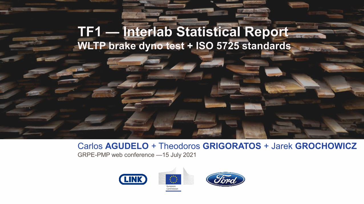
workflow to create the dataset for statistical assessments

WLTP Focus FA single setup 8 labs 2 tests each 6 x WLTP / test~260k values

8 labs x 2 tests x 6 repeats x 303 events x 11 parameters: braking speed, avg. dist. (torque, pressure, and COF), max. disc temps., cooling air temp. & cooling air RH

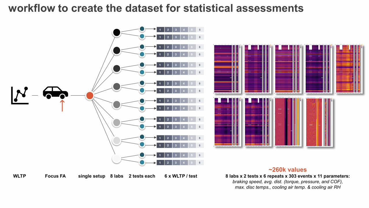
chapters and structure of the report

I. Rationale and justification

Introduction OverviewBackground of ILS-TF1Main lab elementsTest cycle

II. General statistical evaluation

Aggregate stats on speed & decelerationTemperature studySpecial temperature assessment

III. Statistics on time-resolved – EED

General conceptsVDA 305/EKB 3008Speed control: violations & RMSSE

IV. Statistics on event-based – EEC

VDA 305/EKB 3008ISO 5725-5 elementsRepeatability, lab, sample, and total reproducibility std. dev.Data scrutinyUncertainty on estimates sr and sR

IAnnexes (dataviz)

1. Heatmaps2. Flowcharts3. Std. dev. v avg.4. Std. dev. v. event5. Uncertainties (r & R)6. Mandel’s h* (avg.)7. Mandel’s k* (range)8. Mandel’s k* (test)

10 % 45 %20 %~10 %~15 %

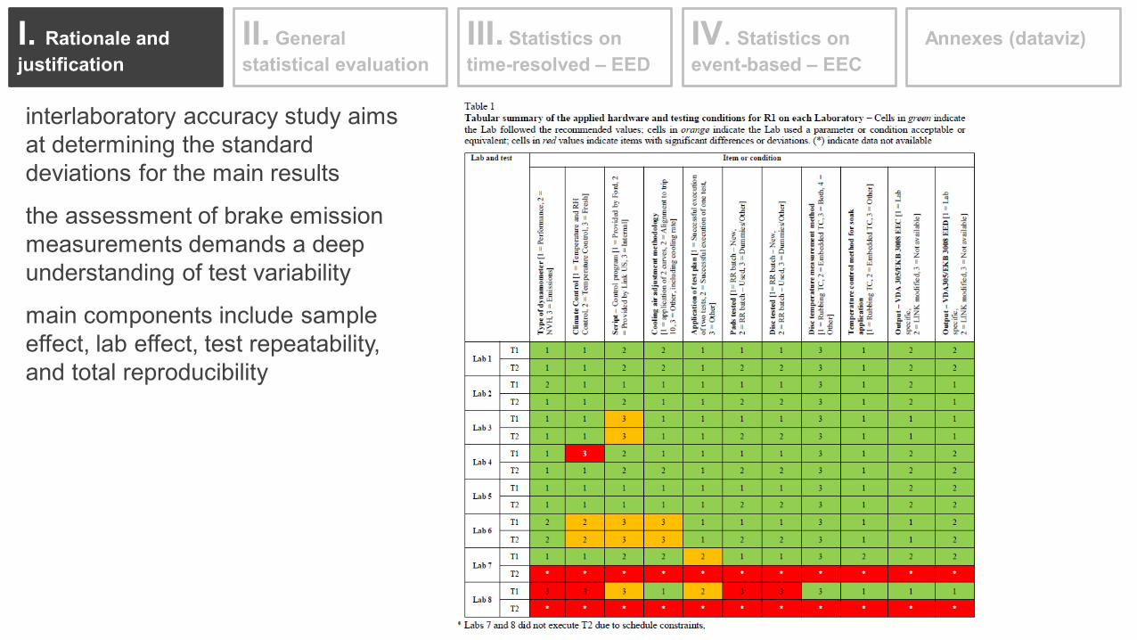
interlaboratory accuracy study aims at determining the standard deviations for the main results

the assessment of brake emission measurements demands a deep understanding of test variability

main components include sample effect, lab effect, test repeatability, and total reproducibility




IAnnexes (dataviz)I. Rationale and justification

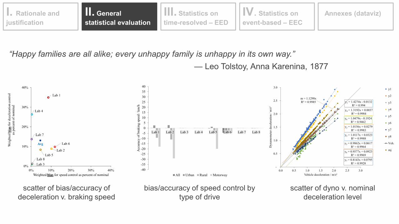
“Happy families are all alike; every unhappy family is unhappy in its own way.”— Leo Tolstoy, Anna Karenina, 1877

scatter of bias/accuracy of deceleration v. braking speed

bias/accuracy of speed control by type of drive

scatter of dyno v. nominal deceleration level





-40-35-30-25-20-15-10-505

10152025303540

Lab 1 Lab 2 Lab 3 Lab 4 Lab 5 Lab 6 Lab 7 Lab 8

Acc

urac

y of

bra

king

spee

d / k

m/h

All Urban Rural Motorway

y1 = 1.4274x - 0.0132R² = 0.994

y2 = 1.0156x + 0.0279R² = 0.9983

y3 = 0.9862x + 0.0617R² = 0.9964

y4 = 1.3192x + 0.0037R² = 0.9984

y5 = 1.0117x + 0.0323R² = 0.9988

y6 = 1.0479x - 0.1924R² = 0.9462

y7 = 0.8143x + 0.0795R² = 0.9928

y8 = 0.9577x + 0.0923R² = 0.9969

m = 1.1298xR² = 0.9985

-

0.5

1.0

1.5

2.0

2.5

3.0

0.0 0.5 1.0 1.5 2.0 2.5 3.0

Dyn

amom

eter

dec

eler

atio

n / m

/s²

Vehicle deceleration / m/s²

y1

y2

y3

y4

y5

y6

y7

y8

Veh.

mj

IAnnexes (dataviz)

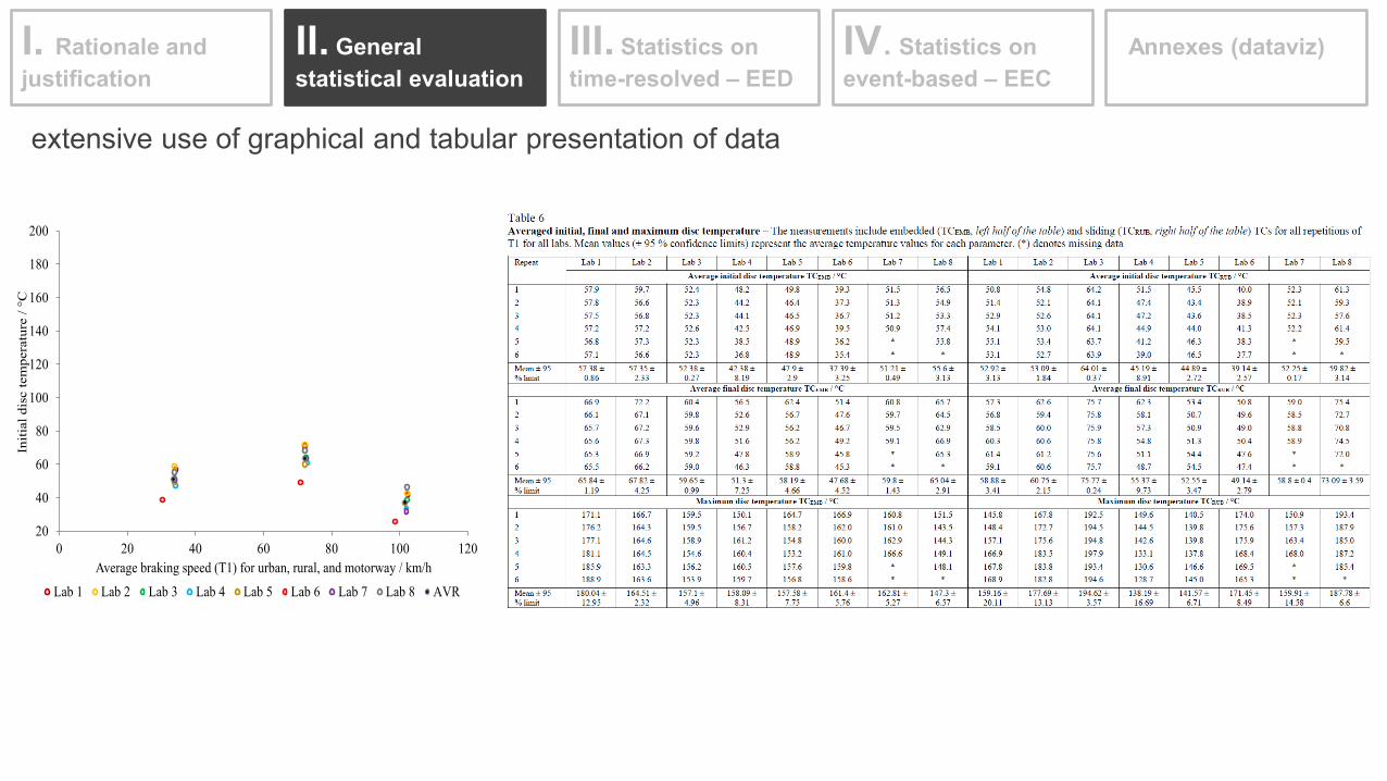
extensive use of graphical and tabular presentation of data





20

40

60

80

100

120

140

160

180

200

0 20 40 60 80 100 120

Initi

al d

isc

tem

pera

ture

/ °C

Average braking speed (T1) for urban, rural, and motorway / km/hLab 1 Lab 2 Lab 3 Lab 4 Lab 5 Lab 6 Lab 7 Lab 8 AVR

IAnnexes (dataviz)

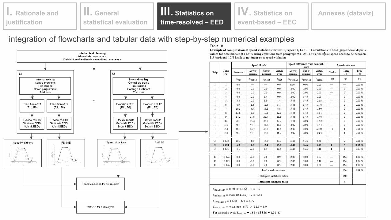
integration of flowcharts and tabular data with step-by-step numerical examples





IAnnexes (dataviz)

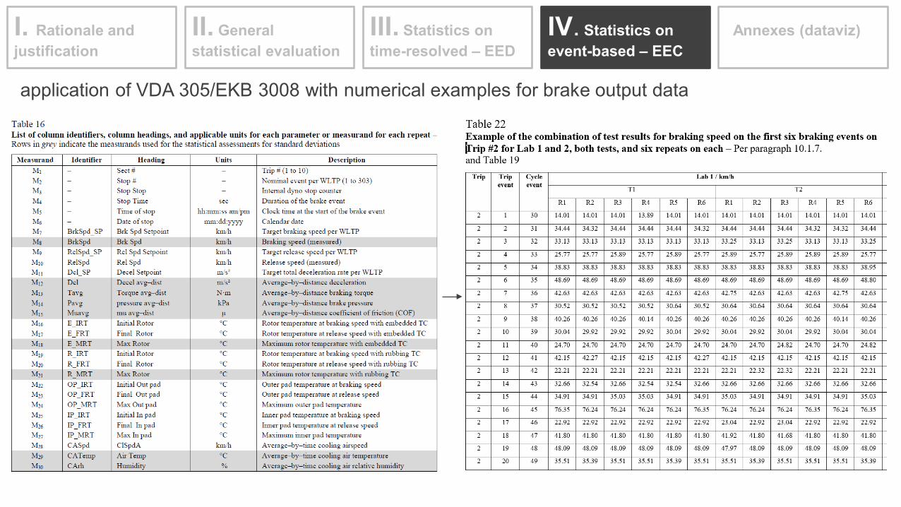
application of VDA 305/EKB 3008 with numerical examples for brake output data





IAnnexes (dataviz)

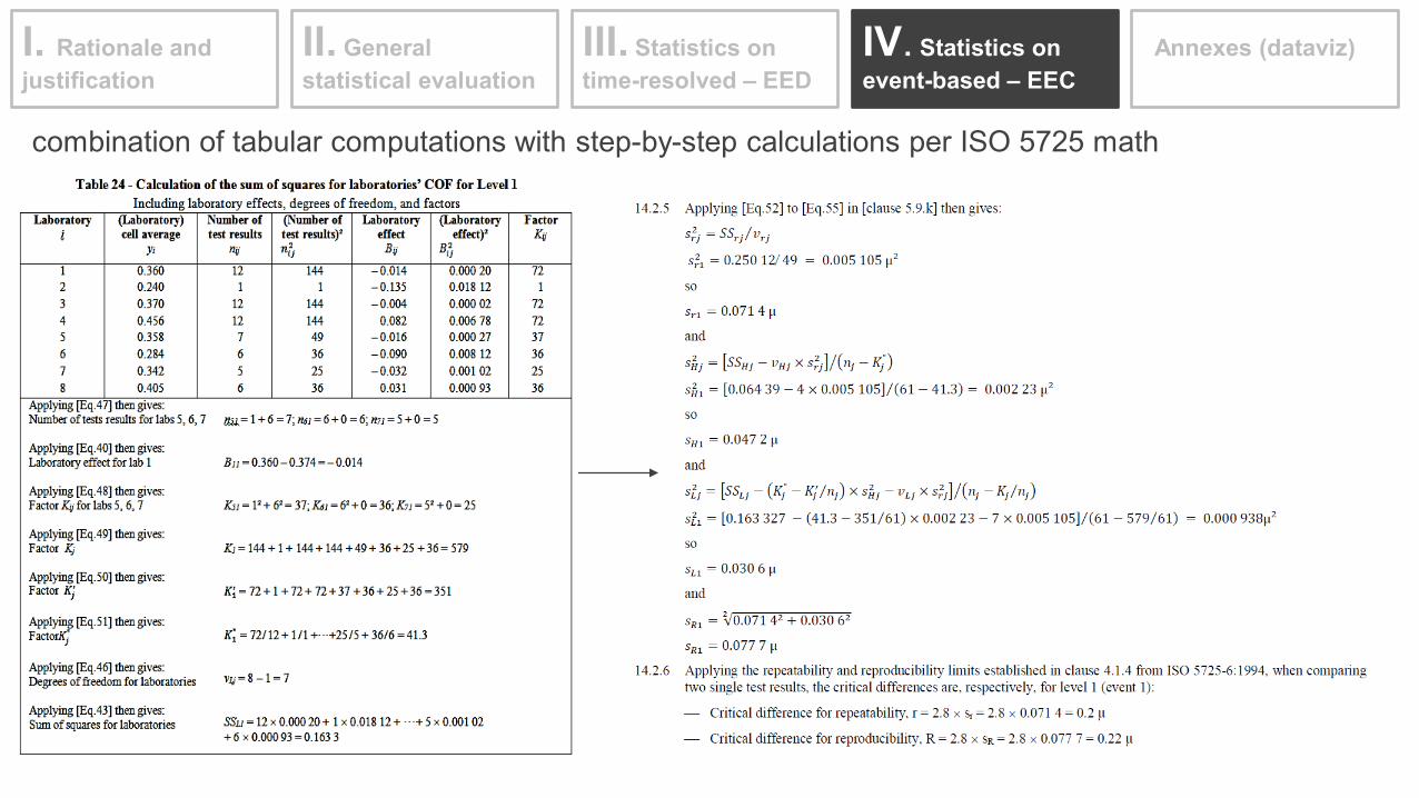
combination of tabular computations with step-by-step calculations per ISO 5725 math





IAnnexes (dataviz)





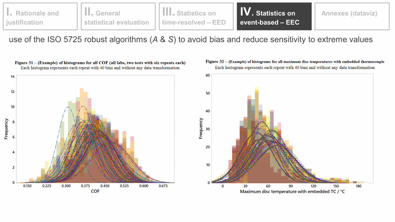
use of the ISO 5725 robust algorithms (A & S) to avoid bias and reduce sensitivity to extreme values

IAnnexes (dataviz)

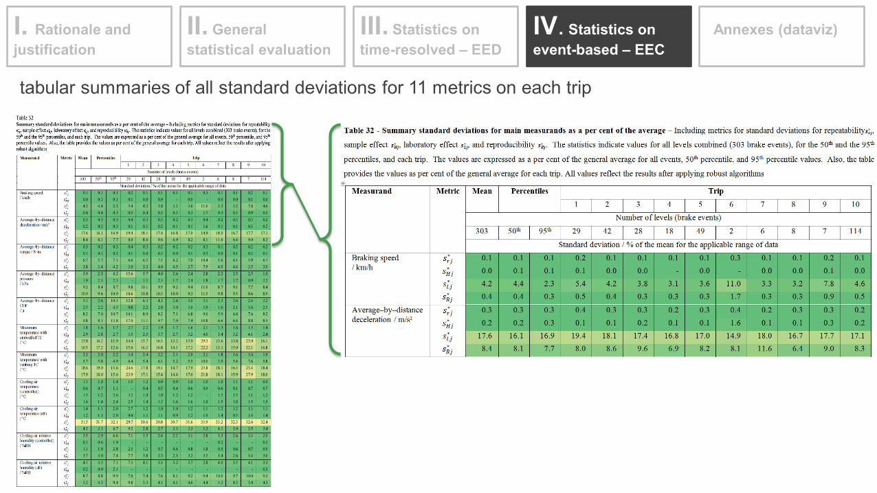
tabular summaries of all standard deviations for 11 metrics on each trip





IAnnexes (dataviz)

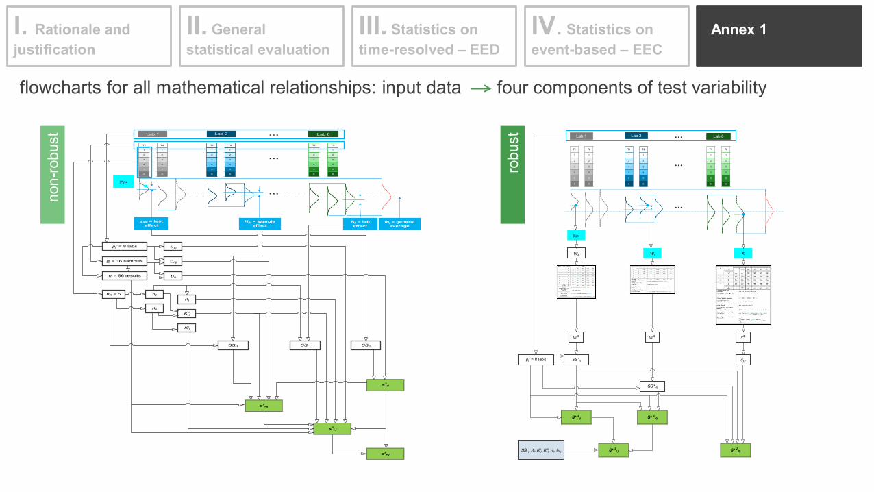
flowcharts for all mathematical relationships: input data four components of test variability





IAnnex 1

T1

1

2

3

4

5

6

T1

1

2

3

4

5

6

T1

1

2

3

4

5

6

T2

1

2

3

4

5

6

T2

1

2

3

4

5

6

T2

1

2

3

4

5

6

m = general average

zijtk = test effect

Lab 1 Lab 8Lab 2 …

…

…

Hijt = sample effect

Bij = lab effect

pj’ = 8 labs

gj = 16 samples

nj = 96 results

nijt = 6

υLj

υHj

υrj

nij

Kij

Kj

K”j

K’j

SSHj SSLj SSrj

zijtk = test effect

Hijt = sample effect

s2Hj

s2rj

s2Lj

s2Rj

Bij = lab effect

yijtk

mj = general average

T1

1

2

3

4

5

6

T1

1

2

3

4

5

6

T1

1

2

3

4

5

6

T2

1

2

3

4

5

6

T2

1

2

3

4

5

6

T2

1

2

3

4

5

6

Lab 1 Lab 8Lab 2 …

…

…

pj’ = 8 labs

yij tk

s*

SSLj, Kj, K’j, K”j, nj, υLj

SS*rj

S* 2HjS* 2

rj

S* 2Lj S* 2

Rj

wit wi xi

w* w*

SS*Hj

syj

non-

robu

st

robu

st

IAnnex 2

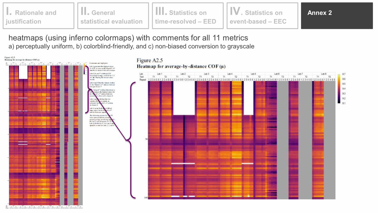
heatmaps (using inferno colormaps) with comments for all 11 metricsa) perceptually uniform, b) colorblind-friendly, and c) non-biased conversion to grayscale





IAnnex 3-5

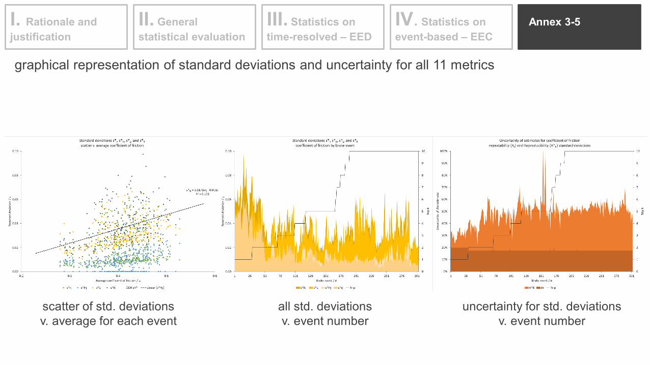
graphical representation of standard deviations and uncertainty for all 11 metrics

scatter of std. deviations v. average for each event

all std. deviations v. event number

uncertainty for std. deviations v. event number





IAnnex 6-8

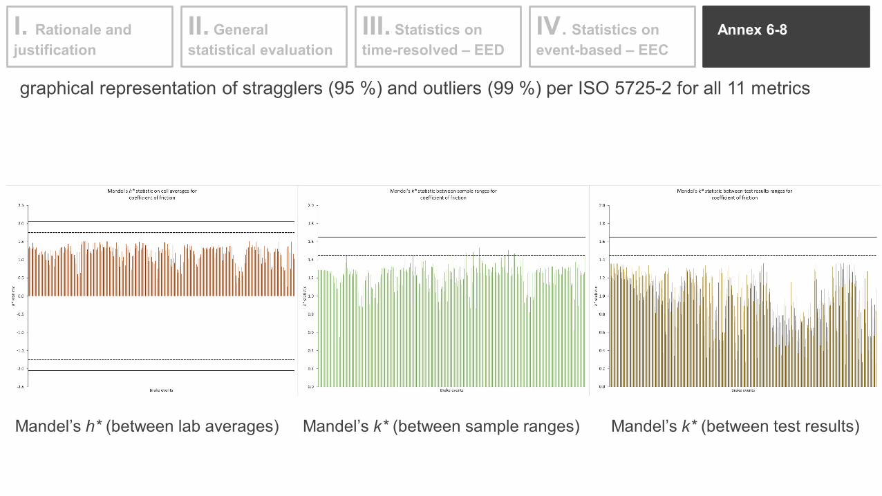
graphical representation of stragglers (95 %) and outliers (99 %) per ISO 5725-2 for all 11 metrics

Mandel’s h* (between lab averages) Mandel’s k* (between sample ranges) Mandel’s k* (between test results)





…what is possible for TF3 – ILS establish critical differences for key dyno metrics(speed, deceleration, cooling air)

PMP 47th, May 16-17, 2018

Special thanks to:Marcel MATHISSENRaviTeja VEDULA + Alejandro HORTET

"Statistical Assessment and Temperature Study from the Interlaboratory Application of the WLTP – Brake Cycle" https://www.mdpi.com/2073-4433/11/12/1309

https://www.mdpi.com/2073-4433/11/12/1309

Documents

TF1 — Interlab Statistical Report