Tests of the Missionland dataset - FFI · PDF fileJTLS the terrain is represented as a grid of hexagons. To cover Missionland and neighbouring ocean areas, the hexagon size was set

FFI-rapport 2013/00391

Tests of the Missionland dataset

Arild Skjeltorp

Norwegian Defence Research Establishment (FFI)

11 February 2013

2 FFI-rapport 2013/00391

FFI-rapport 2013/00391

123301

P: ISBN 978-82-464-2211-4

E: ISBN 978-82-464-2212-1

Keywords

Visualisereng

Simulering

Databaser

Geografi

Topologi

Approved by

Karsten Bråthen Project Manager

Anders Eggen Director

FFI-rapport 2013/00391 3

English summary

The objective of the NATO Science and Technology Organization Task Group MSG-071

“Missionland” is to construct a dataset from which simulation environment databases can be

created. FFI is planning to use the dataset. As a first test a small subset of the dataset has been

used to create a simple visual database using Terra Vista. In order to create a low resolution Joint

Theater Level Simulation terrain, a resampling of the Missionland dataset have been performed.

The resampled low resolution Missionland elevation data have been integrated into a real world

dataset, since a larger area than the area covered by the Missionland dataset was needed to create

the Joint Theater Level Simulation terrain.


Sammendrag

NATO STO MSG-071 “Missionland” har som mål å lage et komplett sett med kildedata som kan

benyttes til å lage syntetisk miljø for bruk til simulering for trening og øving. Fra disse kildedata

vil det kunne lages databaser både for visualisering og for simulering. Denne rapporten beskriver

eksempel på bruk av første versjon av dette datasettet for å lage en visuell database for et område

som har data med høy oppløsning, og et eksempel på en terrengdatabase med relativ lav

oppløsning for bruk i “Joint Theater Level Simulation”.


Contents

1 Introduction 7

2 Visual database created from high resolution Missionland data 7

2.1 Elevation data 8

2.2 Feature data 8

2.3 Building a database in Terra Vista 9

2.4 Use of imagery data in Terra Vista 12

3 Joint Theater Level Simulation terrain 15

3.1 Resampling and integrating Missionland elevation data with real world

data. 15

3.2 Populating a JTLS terrain with elevation data 17

3.3 Use of Missionland vector data 18

4 Conclusion 20

References 21

Abbreviations and acronyms 22

Appendix A GeoTIFF elevation metadata example 23

Appendix B Adding FACC data to shapefiles 24

B.1 Extract of first 29 entries in the feature mapping worksheet 24

B.2 Python Script used to add FACC attributes to Missionland feature data 25

B.3 Python script: dirEntries.py 27

Appendix C GeoTIFF resampling scripts 29

C.1 Python script creating a Global Mapper script 29

C.2 Global Mapper script created from Python 30



1 Introduction

The objective of the NATO Science and Technology Organization Task Group MSG-071

“Missionland” [1] is to construct a dataset from which simulation environment databases can be

created. The scope of the group was to provide a static environmental representation of a

substantial geographical area for use within NATO and NATO Partnership for Peace countries.

A dataset with different geologies, climate and feature types enables for use within a wide range

of simulation systems.

FFI is planning to use the Missionland dataset. As a first test a small subset of the dataset has

been used to create a simple visual database using Terra Vista [2]. The tests have been done with

different versions of the dataset, due to ongoing work in MSG-071. A Joint Theater Level

Simulation (JTLS) [3] terrain have also been created from a resampled Missionland dataset. In

JTLS the terrain is represented as a grid of hexagons. To cover Missionland and neighbouring

ocean areas, the hexagon size was set to 4 km.

2 Visual database created from high resolution Missionland data

The temperate island highlighted in Figure 2.1 shows the part of the Missionland dataset used to

create a visual database in Terra Vista. This island represents one of the more detailed areas of the

Missionland dataset. The first downloaded dataset had no imagery, but that has been added to the

latest version (dataset-v1).

The cells were delivered with the following data:

A Elevation data

o Georeferenced Tagged Image File Format (GeoTIFF ) with 0.0002778 arc

degrees resolution1 (~ 30 m)

B Feature data

o ESRI2 Shapefiles [4] with point, line or area feature data

No imagery data were available for the cells, but a library with 3D models, basic textures, airport

templates and a feature library database was provided. The feature library database is a Microsoft

Access database with data tables containing description of the feature library. This database holds

the Missionland specific feature attribute mapping to common schemas as SEDRIS

Environmental Data Coding Specification (EDCS) [5], Feature and Attribute Coding Catalogue

(FACC) [6] and Defence Geospatial Information Workgroup (DGIWG) [7] Feature Data

Dictionary (DFDD) [8].

1 Elevation data resolution at equator is 0.002778(2πR)/360 = 30.9245 m, using earth radius

R = 6378137 m (WGS84). 2 Environmental System Research Institute (ESRI

®). http://www.esri.com

http://www.esri.com/


Figure 2.1 The highlighted area is the part of the Missionland dataset tested in Terra Vista.

2.1 Elevation data

The elevation data from the cells was imported into Global Mapper ™ [9], and as an example the

GeoTiff metadata for cell J27 is shown in Appendix A. The MIN ELEVATION value in cell J27

was reported as -32766.713 m, but it should have been set to -733.157 m. This may have impact

on the colouring of different elevations, when displayed in a tool such as Global Mapper. In a

later version of data for cells J27 and K27, incorrect or missing elevation data at the rightmost

edge of the cells were found as shown in Figure 2.2. The incorrect elevation data gives a large

negative number for the MIN ELEVATION value in the metadata.

2.2 Feature data

In order to use the default feature data code selector in Terra Vista the data should have been

assigned FACC values. A Python3 script has been created to add FACC to the existing shape

vector data, based on the ML_FID to FACC mapping found in the Missionland feature library

database. The ML_FID is an attribute that identifies the features in the shapefiles.

3 www.python.org

http://www.python.org/


Figure 2.2 Global Mapper used for visualization of elevation data for cell J27.

The feature data table from the Microsoft Access database was exported to a Microsoft Excel 97

worksheet. The first entries in this worksheet are listed in Appendix B.1. We used the xlrd 4

Python library to read the Excel worksheet. Based on the data from the worksheet, a mapping

from the ML_FID to FACC was found. The osg (osgeo)5 Python library was used to add the

matching FACC value to all elements in the shapefiles. A road that is identified by the attribute

ML_FID = 20, is extended with the new FACC attribute code = AP030. The Python script used

to add this attributes to all features in the shapefiles is given in Appendix B.

2.3 Building a database in Terra Vista

Elevation data and the modified vector data were imported into Terra Vista and a simple visual

database (using default Terra Vista textures) was created. In the Terra Vista build log, a few of

the area features were reported as non-closed areas, but that is not unusual.

The resulting OpenFlight[10] database was imported into MÄK VR-Vantage [11] 3D

visualization software and different parts of the database was examined. Viewed from a high

altitude the database looks reasonable good as shown in Figure 2.3. Zooming into details, some

parts of the database look as shown in Figure 2.4. The default textures in Terra Vista give sharp

edges and large contrasts between different areas of the database.

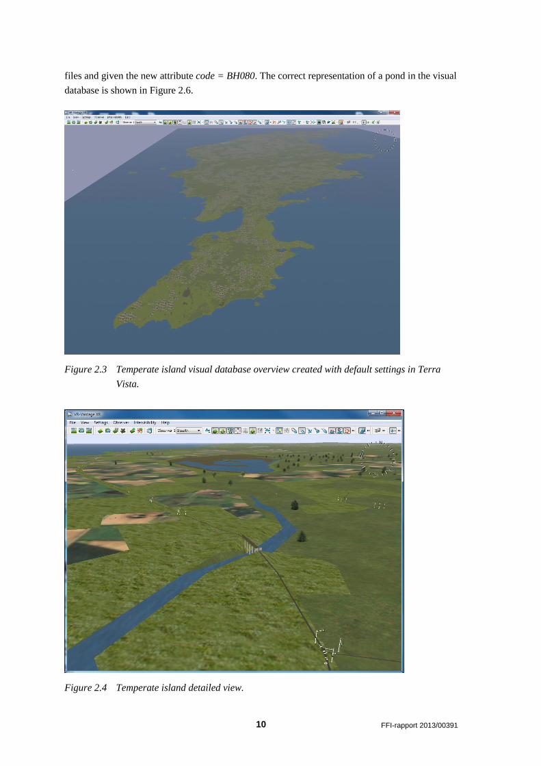
We discovered that lakes and ponds were not created correctly. Since all water surfaces in the

source data are represented as ocean polygons, all water surfaces will be set to sea level (zero

altitude) in the database as shown in Figure 2.5. To get the correct representation of lakes and

ponds in Terra Vista, the lake and pond polygons were manually extracted from the water vector

4 http://pypi.python.org/pypi/xlrd

5http://wiki.osgeo.org/wiki/OSGeo_Python_Library

Lo

wer rig

ht co

rner

http://pypi.python.org/pypi/xlrd

http://wiki.osgeo.org/wiki/OSGeo_Python_Library


files and given the new attribute code = BH080. The correct representation of a pond in the visual

database is shown in Figure 2.6.

Figure 2.3 Temperate island visual database overview created with default settings in Terra

Vista.

Figure 2.4 Temperate island detailed view.


Figure 2.5 Pond represented as ocean surface in Terra Vista.

Figure 2.6 Correct representation of a pond in Terra Vista.


2.4 Use of imagery data in Terra Vista

In the latest version of the dataset, synthetic created imagery data was included as shown in

Figure 2.7. The imagery data has the primary road network included, but no rivers or lakes.

Figure 2.7 Imagery data covering the temperate island in MissionLand.

In Figure 2.8 we can see that there is a mismatch between the imagery and the culture data.

The figure shows the following combination of source data:

(A) Imagery only

(B) Imagery and vector data

o Primary road

o Dirt road

o Rivers

o Lake/pond

o Ocean

(C) Elevation (dark blue areas has zero elevation) and vector data

(D) Imagery, elevation (40% transparency) and ocean (shoreline) vector data


(A) (B)

(C) (D)

Figure 2.8 A more detailed view of the temperate island.

The primary road data is placed correct, but some of the land areas are not defined correct in the

synthetic images. At some locations the correlation is good, but for some areas correlation could

have been better.

In spite of this flaw, the imagery data was imported into Terra Vista, and some of the textures

used in Terra Vista were modified. Selected areas with geotypical textures were blended with the

geospecific texture from the imagery data. This method will reduce the stand out effect from

different terrain areas you can experience, by using geotypical textures only. The result from a

rebuild of the visual database is shown in Figure 2.9.

Some of the differences in the source data can be seen as darker areas along some parts of the

coastline of the island. The vector data defines these areas as land, but the texture from the

imagery indicates that it is ocean. Figure 2.10 shows more details of different areas of the island.

The part of the island shown in Figure 2.8 is the area marked with (3) in Figure 2.10. We can


also see that the northern part of the island (4) has a better match between the different source

data types.

Figure 2.9 Temperate island visual database created in Terra Vista using texture blending.

(1) (2)

(3) (4)

Figure 2.10 Different parts of the temperate island created in Terra Vista using texture blending.


3 Joint Theater Level Simulation terrain

A Joint Theater Level Simulation (JTLS) terrain has been created from the Missionland dataset.

In JTLS the terrain is represented as a grid of hexagons. To cover Missionland and neighbouring

ocean area, the hexagon size was set to 4 km. With a grid size of 932x775, the size of the terrain

in JTLS is approximately 3200 x 3100 km 6 (width x height).

The tool used to populate the hexagons with elevation and sea depth data, uses low resolution

elevation data as input. A Python script was used to create a Global Mapper script for resampling

the whole Missionland elevation dataset to Digital Terrain Elevation Data (DTED) level 0

resolution (0.00833 arc degrees resolution). After running this Global Mapper script, the

resampled GeoTIFF elevation files were imported back into Global Mapper and exported as

DTED level 0 elevation data. The Python and Global Mapper scripts are listed in Appendix C.

A Java based tool for populating a JTLS terrain file with DTED level 0 elevation and depth data

has been made at FFI.

3.1 Resampling and integrating Missionland elevation data with real world data.

From the National Oceanographic and Atmospheric Administration (NOAA) web pages [12] a

global elevation and bathymetry dataset can be downloaded. A world wide 1 arc minute

resolution data set (named ETOPO1) [13] has been resampled and converted to DTED level 0

resolution (0.5 arc minutes). Figure 3.1 shows a colour shaded relief image of the ETOPO1

dataset downloaded from the NOAA web pages.

Figure 3.1 Downloaded colour shaded-relief image visualizing the ETOPO1 dataset.

6

√

= 3228 km , = 3100 km


In order to integrate the newly created low resolution Missionland dataset into the ETOPO1 data,

the dataset had to be edited. First an extended seabed was added around the Missionland

continent, since the outer ocean ring was not present in the downloaded Missionland dataset.

ITED [14] was used to do a quick and simple blending of the extended Missionland data into a

slightly larger area cut out from the ETOPO1 data. The large depth difference between the real

world seabed and the Missionland seabed was a challenge. Figure 3.2 shows the result of this

process. The new dataset was then integrated into the global ETOP1 dataset as shown in Figure

3.3.

Figure 3.2 Missionland with extended seabed (left) and Missionland integrated with an area cut

out from the ETOPO1 dataset (right).

Figure 3.3 Missionland integrated into the ETOPO1 dataset.


3.2 Populating a JTLS terrain with elevation data

A JTLS terrain is defined by two text files. The terrain definition file defines the Lambert

conformal map projection parameters and the size of the area covered. The terrain file holds the

data for each hexagon and the six hexagon borders. A Java based application has been developed

at FFI to set the terrain type based on the elevation or depth read from a DTED level 0 dataset.

The land terrain type is set to a type depending on the terrain height found in the center position

of the hexagon. Low terrain is set to an open terrain type; medium terrain is set to forest, and high

terrain as mountain as shown in Figure 3.4. An outline of the JTLS terrain area is shown in Figure

3.5.

Figure 3.4 JTLS terrain type and depth/elevation is set based on resampled DTED level 0.

Figure 3.5 The area covered in the JTLS terrain is outlined.


3.3 Use of Missionland vector data

The use of the original Missionland vector data in JTLS was found to be difficult, since the data is

organized as separate vector data for each of the geocells. A Python script was created to copy

one specified feature type (e.g. road) from the shapefiles in all cells, into one single shape file

covering the whole Missionland continent. As an example, the road data was simplified and

incorporated into the JTLS terrain as shown in Figure 3.6.

Figure 3.6 JTLS terrain with road network.

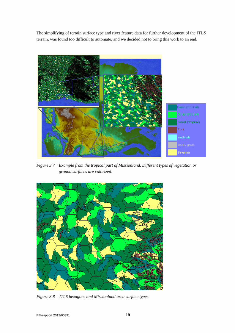
For some of the other feature types the extraction and simplifying of the data, turned out to be a

difficult task. The different land use and vegetation types consist of a very large number of small

areas as shown in Figure 3.7. That makes it much more difficult to create the coarse data needed

to set the corresponding terrain type in the JTLS terrain hexagons as shown in Figure 3.8.

The river vectors are also difficult to simplify since they are composed of a large number of small

segments. A total of 15,751,839 river segments were found in the shape data. In Figure 3.9 one

river segment is selected, and the feature information about this segment tell us that this feature is

only 61.521 m long and only has two vertices. It would have been better to have larger segments

with several vertices. The areas which are based on real world data have such river segments. In a

JTLS terrain the rivers have to be defined to run along one of the borders of the hexagons.


The simplifying of terrain surface type and river feature data for further development of the JTLS

terrain, was found too difficult to automate, and we decided not to bring this work to an end.

Figure 3.7 Example from the tropical part of Missionland. Different types of vegetation or

ground surfaces are colorized.

Figure 3.8 JTLS hexagons and Missionland area surface types.


Figure 3.9 River segment information.

4 Conclusion

The first impression from our tests of the Missionland dataset is that this is a good start on the

road to create a complete dataset that can be used as source data to create non geospecific

simulation environment databases. The use of the data for a specific purpose will identify any

improvements that have to be done to make the dataset even more complete. This report describes

two different uses of the dataset. The first example shows the use of high resolution data to create

a visual database, and the second example an attempt to create a low resolution JTLS terrain

database. To complete the creation of the JTLS terrain, further work has to be done.

Some shortcomings have been discovered during these tests:

The outer ring that integrates Missionland into real world data is missing.

Correlation between imagery, elevation and vector data.

Ocean and lakes should have different ML_FID values.

Different types of land use should consist of larger coherent areas.

Longer river segments should have been created.


References

[1] NATO STO, "STO Task Group MSG-071- Missionland Final Report (Draft)", NATO

STO, 2012.

[2] Presagis, "Terra Vista", (2010). [Online]. Available:

http://www.presagis.com/products_services/products/modeling-

simulation/content_creation/terra_vista

[3] Rolands & Associates Corporation, "Joint Theatre Level Training Simulation (JTLS)",

(2008). [Online]. Available: www.jtls.com.

[4] ESRI, "ESRI Shapefile Technical Description", (1-7-1998). [Online]. Available:

http://www.esri.com/library/whitepapers/pdfs/shapefile.pdf

[5] NATO NSA, "SEDRIS - Environmental Data Coding Specification (ECDS), STANAG

4662 (Edition 1)", (Unclassified - Unlimited), 2008.

[6] DGIWG, "The Digital Geographic Information Exchange Standard (DIGEST) - Part4

FEATURE and ATTRIBUTE CODING CATALOGUE (FACC)", DGIWG, Sept. 2000.

[7] DGIWG, "Defence Geospatial Information Working Group website", (2013). [Online].

Available: www.dgiwg.org

[8] DGIWG, "Implemention guide to the DGIWG Feature Data Dictionary (DFDD)", DGIWG,

Jan. 2010.

[9] Global Mapper Software LLC, "Global Mapper website", (2011). [Online]. Available:

www.globalmapper.com

[10] Presagis, "OpenFlight Scene Description Database Specification, Document Revision A,

Version 16.4, June 2009", 2009.

[11] MÄK Technologies, "VR-Vantage Stealth", (2011). [Online]. Available:

http://www.mak.com/products/visualize/3d-simulation-visualization.html.

[12] NOAA, "National Oceanographic and Atmospheric Administration website", (2013).

[Online]. Available: http://www.ngdc.noaa.gov/mgg/global/global.html

[13] C. Amante and B. W. Eakins, "ETOPO1 1 Arc-minute global relief model : Procedures,

data sources and analysis", NOAA, Mar. 2009.

[14] M. F. Aasen and L. H. Breivik, "Interactive Terrain Editor (ITED)", Forsvarets

forskningsinstitutt, FFI-rapport 2011/01216, June 2011.

[15] MSG-071, "MSG-071- Missionland Contribution Guide (Draft)", NATO STO, Version 0.5,

Aug. 2012.

http://www.presagis.com/products_services/products/modeling-simulation/content_creation/terra_vista

http://www.presagis.com/products_services/products/modeling-simulation/content_creation/terra_vista

http://www.jtls.com/

http://www.esri.com/library/whitepapers/pdfs/shapefile.pdf

http://www.dgiwg.org/

http://www.globalmapper.com/

http://www.mak.com/products/visualize/3d-simulation-visualization.html

http://www.ngdc.noaa.gov/mgg/global/global.html


Abbreviations and acronyms

NATO North Atlantic Treaty Organization

STO Science and Technology Organization

MSG Modelling and Simulation Group

ESRI Environmental System Research Institute

FFI Forsvarets forskningsinstitutt (Norwegian Defence Research Establishment)

JTLS Joint Theater Level Simulation

GeoTIFF Georeferenced Tagged Image File Format

FACC Feature and Attribute Coding Catalogue

EDCD Environmental Data Coding Specification

DTED Digital Terrain Elevation Data

DGIWG Defence Geospatial Information Working Group

DFDD DGIWG Feature Data Dictionary

NOAA National Oceanographic and Atmospheric Administration

ITED Interactive Terrain Editor


Appendix A GeoTIFF elevation metadata example

Table A.1 below shows the GeoTIFF elevation metadata reported by Global Mapper for cell J27.

FILENAME MissionLand\geocells\J27_W38_N33\Elevation\J27_W38_N33.tif

DESCRIPTION J27_W38_N33.tif

UPPER LEFT X -38.0000000000

UPPER LEFT Y 34.0000000000

LOWER RIGHT X -37.0000000000

LOWER RIGHT Y 33.0000000000

WEST LONGITUDE 38.00000000° W

NORTH LATITUDE 34.00000000° N

EAST LONGITUDE 37.00000000° W

SOUTH LATITUDE 33.00000000° N

PROJ_DESC Geographic (Latitude/Longitude) / WGS84 / arc degrees

PROJ_DATUM WGS84

PROJ_UNITS arc degrees

EPSG_CODE 4326

COVERED AREA 10322 sq km

NUM COLUMNS 3601

NUM ROWS 3601

NUM_BANDS 1

PIXEL WIDTH 0.0002778 arc degrees

PIXEL HEIGHT 0.0002778 arc degrees

MIN ELEVATION -32766.713 meters

MAX ELEVATION 29.715 meters

ELEVATION UNITS meters

BIT_DEPTH 32

PHOTOMETRIC Greyscale (Min is Black)

BIT_DEPTH 32

SAMPLE_FORMAT Floating Point

ROWS_PER_STRIP 1

COMPRESSION None

PIXEL_SCALE ( 0.00027777777778, 0.00027777777778, 1 )

TIEPOINTS ( 0.00, 0.00, 0.00 ) --> ( -38.0001388889, 34.0001388889,

0.0000000000 )

MODEL_TYPE Geographic lat-long system

RASTER_TYPE Pixel is Area

VERT_DATUM None Specified

Table A.1 GeoTIFF elevation metadata from Global Mappet


Appendix B Adding FACC data to shapefiles

The Python script in Appendix B.2 reads Missionland feature mapping information from a

Microsoft Excel 97 worksheet and adds FACC data to all features in all shapefiles found in a

directory and all its subdirectories (Appendix B.3). Table B.1 shows an extract of the first entries

in the Excel worksheet. The columns with EDCD and DFDD mapping are removed from the data

shown in Table B.1. The ML_FID attribute value is identical to the value from the ID column in

this worksheet. This script is inspired by the “Update vector attributes” script found in the MSG-

071 Missionland Contribution Guide [15].

B.1 Extract of first 29 entries in the feature mapping worksheet

ID Name Description FeatureType FACCMapping

5 temperate_fields Polygons with field texture for temperate zone AREA EA010

6 rocky_grass Polygon with rocky grass texture AREA EB010

7 rock Polygon with rock texture AREA DB160

8 runway_asphalt Polygon of runway with asphalt texture AREA GB055

9 Mixed forest Polygon with mixed forest canopy texture AREA EC015

10 ocean Polygon with ocean texture AREA BA040

11 silo model of sile POINT AM020

12 cemetery model of cemetery POINT AL030

13 church model of church POINT AL015

14 farm house 3D model of farm house POINT AL015

15 Building footprint Draw building footprint on map AREA AL015

16 Recreational buildings Polygon with recreational buildings texture AREA AI020

17 Orchard Polygon with orchard texture AREA EA040

18 Built-up area Polygon with built-up area texture AREA AL020

19 Wetlands Polygon with wetlands texture AREA BH095

20 Road Extruded line with road texture LINE AP030

21 Cycle path Extrude line with cycle path texture LINE AP050

22 Jetty Extrude line with jetty texture LINE BB140

23 Depth line Depth line on map only LINE BE015

24 Animal welfare area Line on map for animal welfare area LINE AL005

25 Ferry route Ferry route on map LINE AQ070

26 Height line Height line on map POINT CA010

27 Railroad Extruded line with railroad texture LINE AN010

28 River Extrude line with river texture LINE BH140

29 Underground river Underground river, on map only LINE BH115

Table B.1 Feature mapping table


B.2 Python Script used to add FACC attributes to Missionland feature data

'''

Created on 8. nov. 2012

Reads MS-Excel file with Missionland feature data mapping and adds

the matching FACC attribute to all features for all the Shapefiles

in a directory and all its sub directories.

The MS-Excel file with features created by exporting the feature form

from the MS-Access file: ML_feature_library_database.mdb

@author: Arild Skjeltorp, FFI

'''

from xlrd import open_workbook

from osgeo import ogr

import sys

import dirEntries

def find_index(lst, name):

for i in xrange(len(lst)):

if name == lst[i]:

return i

return -1

def find_FACC_code(xl_sheet,ML_FID):

atr_names = []

row = 0

for col in range(xl_sheet.ncols):

atr_names.append(xl_sheet.cell(row,col).value)

fidx = find_index(atr_names,"FACCMapping")

nx = find_index(atr_names,"Name")

if fidx != -1 and nx != -1:

idx = find_index(atr_names,"ID")

if idx != -1:

for row in range(xl_sheet.nrows):

if xl_sheet.cell(row,idx).value == ML_FID:

return [ML_FID, xl_sheet.cell(row,fidx).value, xl_sheet.cell(row,nx).value]

return [ML_FID,"None","Unknown"]


def HasField(layer, field):

layer_defn = layer.GetLayerDefn()

field_names = [layer_defn.GetFieldDefn(i).GetName() for i in range(layer_defn.GetFieldCount())]

return field in field_names

def EnsureFieldExists(layer, field, fieldType):

layer_defn = layer.GetLayerDefn()

field_names = [layer_defn.GetFieldDefn(i).GetName() for i in range(layer_defn.GetFieldCount())]

if not(field in field_names):

new_field = ogr.FieldDefn(field, fieldType)

layer.CreateField(new_field)

if (len(sys.argv) < 3):

print "Please provide MS Excel 97 file and Shape file directory as arguments"

else:

try:

wb = open_workbook(sys.argv[1])

print "Opened excel file: " + sys.argv[1]

# get ML shape attributes form excel sheet. Assume only one Sheet

s = wb.sheet_by_index(0)

print "Sheet name : " + s.name

filelist = dirEntries.dirEntries(sys.argv[2], True, "shp")

for shapefile in filelist:

try:

hShp = ogr.Open(shapefile, 1)

print "Processing shape file: " + shapefile

layer = hShp.GetLayer()

EnsureFieldExists(layer, 'code', ogr.OFTString)

if HasField(layer,'ML_FID'):

feat = layer.GetNextFeature()

numfeatures = layer.GetFeatureCount()

print "Number of features in layer= " + str(numfeatures)

nfeat = 0

nerr = 0

while feat is not None:

mlfid = feat.GetFieldAsInteger('ML_FID')

facc_code = find_FACC_code(s,mlfid);

if (facc_code[1] != 'None'):

try:

feat.SetField('code',str(facc_code[1]))

layer.SetFeature(feat)


nfeat +=1

except:

nerr +=1

feat = layer.GetNextFeature()

layer.SyncToDisk()

hShp = None

print "Changed attribute for " + str(nfeat) + " features"

if (nerr > 0): print "number of errors = " + str (nerr)

except:

print "Unable to open shape file: " + shapefile

except:

print "Unable to open excel file: " + sys.argv[1]

print "Ready"

B.3 Python script: dirEntries.py

import os

def dirEntries(dir_name, subdir, *args):

'''Return a list of file names found in directory 'dir_name'

If 'subdir' is True, recursively access subdirectories under 'dir_name'.

Additional arguments, if any, are file extensions to match filenames. Matched

file names are added to the list.

If there are no additional arguments, all files found in the directory are

added to the list.

Example usage: fileList = dirEntries(r'H:\TEMP', False, 'txt', 'py')

Only files with 'txt' and 'py' extensions will be added to the list.

Example usage: fileList = dirEntries(r'H:\TEMP', True)

All files and all the files in subdirectories under H:\TEMP will be added

to the list.

'''

fileList = []

for file in os.listdir(dir_name):

dirfile = os.path.join(dir_name, file)

if os.path.isfile(dirfile):

if not args:

fileList.append(dirfile)

else:

if os.path.splitext(dirfile)[1][1:] in args:

fileList.append(dirfile)


# recursively access file names in subdirectories

elif os.path.isdir(dirfile) and subdir:

print "Accessing directory:", dirfile

fileList.extend(dirEntries(dirfile, subdir, *args))

return fileList


Appendix C GeoTIFF resampling scripts

The Python script in Appendix C.1 creates a Global Mapper script that imports a GeoTIFF file

and saves a resampled file to a new directory. This action is done for every GeoTIFF file found

in the given directory and all its subdirectories. The first lines of the created Global Mapper script

are shown in Appendix C.2.

C.1 Python script creating a Global Mapper script

# Arild Skjeltorp

import sys

import os

import dirEntries

sys.stdout.write("Generates a Global Mapper script that resamples all tiff-files to 1000m resolution (DTED

level 0)\n")

#check command line arguments

path = "G:\\MissionLand\\current\\geocells"

if len(sys.argv) > 1:

path = sys.argv[1]

ofile = "ML_resample.gms"

#create a list of .tif files in ‘path’ and all its subdirectories

fileList = dirEntries.dirEntries(path, True, "tif")

outfile = open(ofile,'w')

outfile.write("GLOBAL_MAPPER_SCRIPT VERSION=1.00\nUNLOAD_ALL\n")

outfile.write("// Resample to 1000m resolution \n")

for fname in fileList:

out_fname = os.path.basename(fname)

print out_fname

outfile.write("IMPORT FILENAME=\"%s\"\n" % (fname))

outfile.write("EXPORT_ELEVATION FILENAME=\"resampled\\%s\" TYPE=GEOTIFF

SPATIAL_RES=0.00833,0.00833 \n" % (out_fname))

outfile.write("UNLOAD_ALL\n")

outfile.close()


C.2 Global Mapper script created from Python

GLOBAL_MAPPER_SCRIPT VERSION=1.00

UNLOAD_ALL

// Resample to 1000m resolution

IMPORT FILENAME="G:\MissionLand\current\geocells\E10_W55_N38\Elevation\E10_W55_N38.tif"

EXPORT_ELEVATION FILENAME="resampled\E10_W55_N38.tif" TYPE=GEOTIFF

SPATIAL_RES=0.00833,0.00833

UNLOAD_ALL

IMPORT FILENAME="G:\MissionLand\current\geocells\E11_W54_N38\Elevation\E11_W54_N38.tif"

EXPORT_ELEVATION FILENAME="resampled\E11_W54_N38.tif" TYPE=GEOTIFF

SPATIAL_RES=0.00833,0.00833

UNLOAD_ALL

.

.

.

Documents

Tests of the Missionland dataset - FFI · PDF fileJTLS the terrain is represented as a grid of hexagons. To cover Missionland and neighbouring ocean areas, the hexagon size was set