Testing the formation of extended star clusters · Testing the formation of extended star clusters Paolo Bianchini (MPIA, Heidelberg) Florent Renaud, Mark Gieles & Anna Lisa Varri

Testing the formation of extended star

clustersPaolo Bianchini (MPIA, Heidelberg)

Florent Renaud, Mark Gieles & Anna Lisa Varri

MNRAS 447, L40-L44 (2015)

The zoo of small stellar systemsAIMSS I 15

−5 −10 −15 −20 −25MV [mag]

1

10

100

1000

10000R

e [pc

]

EsATLAS3D

dEs/dS0s

dSphscEsAIMSS w/o m

AIMSS with mNucleiGCs/UCDs

YMCsM32

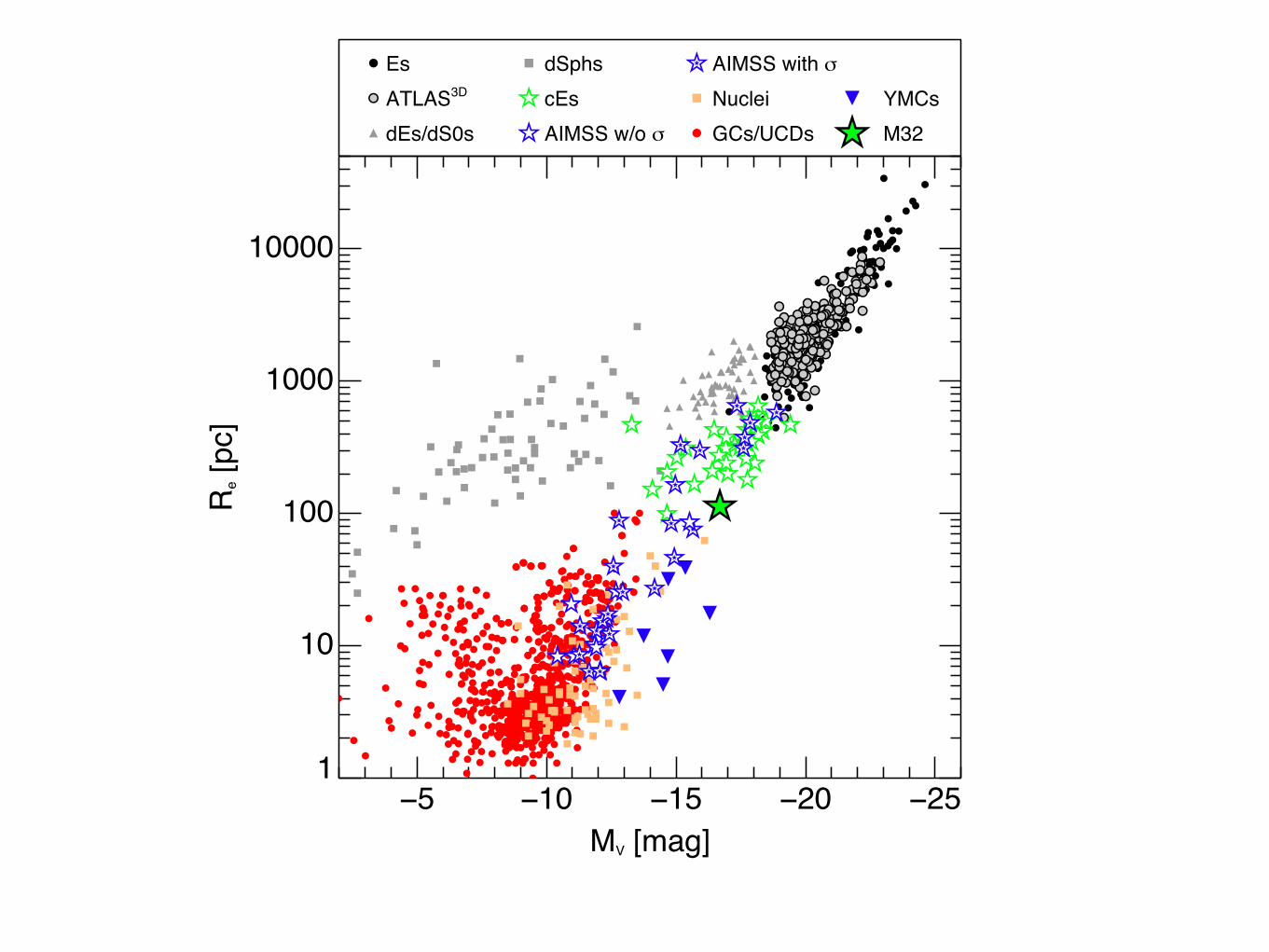
Figure 11. E↵ective radius Re vs absolute V-band magnitude MV for dynamically hot stellar systems from our master compilation.Blue stars are our observations and are filled where we have successfully measured the velocity dispersion of the object. M32 is indicatedby its own symbol and labelled. It is clear that the group of six (including one literature Coma cE) non-YMC objects with MV < –14and Re < 100pc lie o↵set significantly from the more massive previously known UCDs such as Virgo-UCD7 and Fornax-UCD3, whichare smaller than M32.

are tidally stripped from the simulations of Pfe↵er & Baum-gardt (2013). The simulations are numbers 3 (brown) and 17(orange) from Pfe↵er & Baumgardt (2013). They are bothof dE,N galaxies on elliptic orbits with apocenter of 50 kpcand pericenter of 10 kpc around a cluster centre which hasproperties chosen to match M87 in the Virgo cluster. Simu-lation 3 originally has a nucleus with Re = 4 pc and MV =–10, Simulation 17 initially has a nucleus with Re = 10 pcand MV = –12. Both are simulated for a total of 4.2 Gyr.We use these simulations to stand in for simulations of any

nucleated dwarf galaxies undergoing stripping, as at presentvery few simulations of the stripping of later type dwarfshave been carried out, but we expect that the stripping ofother dwarf galaxy types should produce reasonably simi-lar results. The simulations of Pfe↵er & Baumgardt (2013)demonstrate that the remnants of the stripping of dE,Ns canresemble almost all massive GCs and UCDs, even the mostextended (Re ⇠ 100pc) and massive (M ⇠ 108 M�) UCDssuch as Fornax-UCD3, Virgo-UCD7, and Perseus-UCD13.However, it is also clear that these simulations cannot re-

c� 2014 RAS, MNRAS 000, 1–25

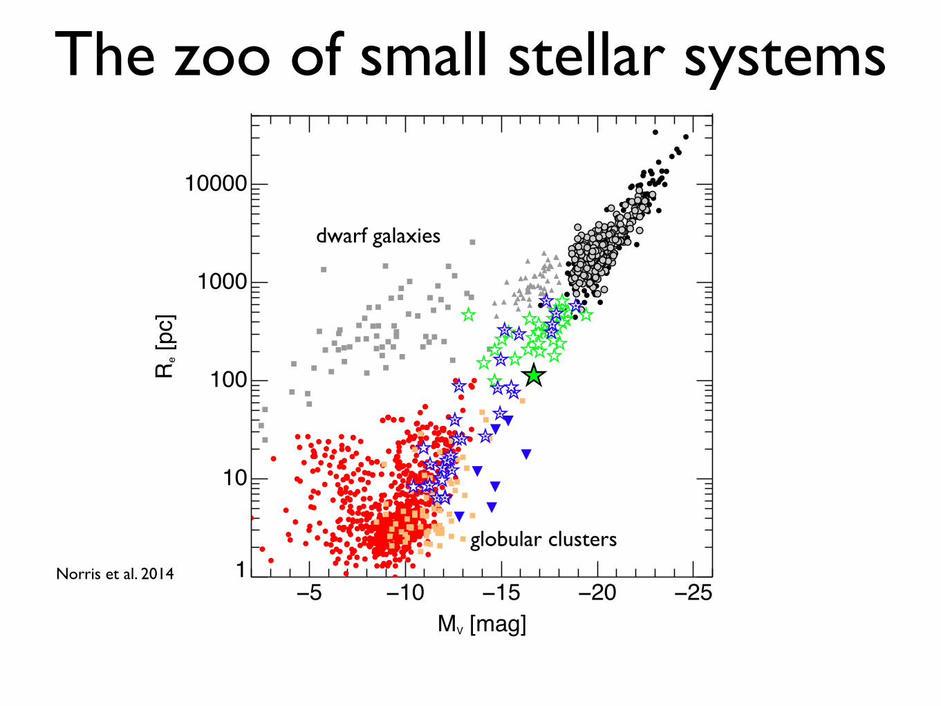
Norris et al. 2014

dwarf galaxies

globular clusters

Leaman, VandenBerg & Mendel (2013)

in-situ MW disk

Age

[G

yr]

[Fe/H]

In-situ GCs

• GCs in disk-like orbits, consistent with age-metallicity of MW disk

Accreted GCs

• 2/3 of GCs in halo-like orbits

• accreted as part of 107-108 M� disrupted dwarf host galaxies

decreasing host halo

Origin of galactic GCs?

Laevens 1 / Crater

Laevens et al. 2014:- “most distant MW cluster”

Belokurov et al. 2014:- “dwarf galaxy with unusual properties”

A new distant distant Milky Way globular cluster 3

Figure 1. Left panels: a): The CMD of PS1 stars within 3 half-light radii of the centroid of PSO J174.0675-10.8774. b): The CMD ofstars of a nearby field region (8.3 arcminutes North-East away) of the same coverage. c): WFI stars within 2 half-light radii of the centroidof PSO J174.0675-10.8774. d): WFI stars within 2 half-light radii of the aforementioned field region. The CMD of the new GC shows aclear RGB, HB, and grazes its main sequence turn-o! at the faint end. Right panels: e): The CMD of PSO J174.0675-10.8774 with theParsec isochrone of age 8Gyr and [Fe/H] = !1.9 that matches the shape and location of the RGB, HB, and main sequence turn o!. g):The spatial distribution of the WFI stars, displaying the unambiguous overdensity produced by PSO J174.0675-10.8774. The red circleshows the region within 2 half-light radii of its centroid. f, h): CMDs within two half-light radii of young outer halo GCs Pal 14 and Pal4, shifted to the distance of the new GC. This photometry is taken from Saha et al. (2005). The CMDs of these two stellar systems showmany similarities with that of PSO J174.0675-10.8774, especially their red HBs and sparsely populated RGBs.

Figure 2. BV R image of PSO J174.0675-10.8774 built from thestacked WFI images. The image is 4! " 4!, north is to the top andeast to the left.

and [Fe/H] = !1.9. Allowing the distance to vary withinthe formal distance uncertainties, we obtain a metallicityand age range of 8–10 Gyrs and [Fe/H] varies between

!1.5 and !1.9. These are fairly typical properties ofyoung, outer halo GCs and this impression is further bol-stered by panels f and h of Figure 1, which present liter-ature photometry (Saha et al. 2005) of Pal 14 (11.3Gyr,[Fe/H] = !1.5; Dotter et al. 2011) and Pal 4 (10.9Gyr,[Fe/H] = !1.3) shifted to the distance of the new GC.The CMDs of the three GCs exhibit similar features, withsparsely populated RGBs and red HBs.To determine the structural parameters of PSO

J174.0675-10.8774, we use a variant of the technique pre-sented in Martin et al. (2008), updated to allow for a fullMarkov Chain Monte Carlo treatment. Briefly, the algo-rithm uses the location of every single star in the WFIdata set to calculate the likelihood of a family of radialprofiles with flattening and a constant background. Theparameters are: the centroid of the system, its elliptic-ity8, the position angle of its major axis from N to E,the number of stars in the system, and one or two scaleparameters. We use three di!erent families of radial den-sity models (exponential, Plummer, and King), for whichthe scale parameters are the half-light radius, the Plum-mer radius, and the core and King radii, respectively.The resulting structural parameters are listed in Table 1.Figure 3 also shows the probability distribution function(pdf) of the exponential model parameters, as well asthe comparison between the favored radial distributionprofile and the data, binned with the favored structuralparameter model. They show a very good agreement,

8 The ellipticity is here defined as 1!b/a with a and b the majorand minor axis scale lengths, respectively.

Laevens et al. 2014

GC or dwarf galaxy?

The zone of confusion

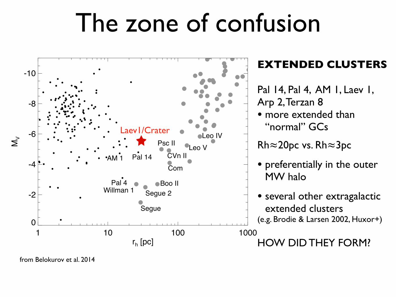
from Belokurov et al. 2014

4 Belokurov et al.

-0.5 0.0 0.5 1.0 1.5 2.0g-i

26

24

22

20

18

16

i

-2.5-2.0 -1.5

160 350 1000m-M=21.1α/Fe=0.4

-0.5 0.0 0.5 1.0 1.5 2.0g-i

26

24

22

20

18

16

i

Figure 6. Colour magnitude diagram of the Crater stars within 2rh of the center. Left: All WHT ACAM sample A stars inside two half-light radii. Forcomparison, 7 and 10 Gyr and [!/Fe] = 0.4 Dartmouth isochrones with metallicities [Fe/H]=!2.5 (blue), [Fe/H]=!2.0 (green) and [Fe/H]=!1.5 (red) areover-plotted. Also shown are 160 Myr (black), 350 Myr (dark grey) and 1 Gyr (light grey) Padova isochrones. If the RC distance calibration is trustworthy,then the bulk of Crater’s stellar population is old (between 7 and 10 Gyr) and metal-poor (!2.5 < [Fe/H] < !2.0). However, there are three peculiar stars,two directly above the blue side of the Red Clump and one at g ! i " 0.3 and i " 19 that can be interpreted as Blue Loop giants. If this interpretation iscorrect, then according to the Padova isochrones, Crater has experienced a small amount of star-formation around 1 Gyr ago and perhaps as recently as 350Myr ago. Right: Hess difference between the CMD densities of the stars inside rh and the stars outside 4.5rh. Note the tightness of the sub-giant region.

1 10 100 1000rh [pc]

0

-2

-4

-6

-8

-10

MV

Segue 2

Segue

Boo IIWillman 1

CVn IICom

Psc IILeo IV

Leo V

Crater

AM 1

Pal 4

Pal 14

Figure 5. LuminosityMV versus half-light radius rh for Galactic globularclusters (black dots) and Milky Way and M31 satellites (grey circles). Thered star marks the location of Crater. The new satellite appears to have morein common with the Galactic globular cluster population, even though it ap-pears to be the largest of all known Milky Way globulars. Contrasted withthe known ultra-faint satellites, Crater is either too small for the given lumi-nosity, c.f. Pisces II, Leo V or too luminous for a given size, c.f. Willman 1,Segue.

cessed to that date (! 2700 square degrees). The satellite stoodout as the most significant candidate detection, as illustrated by thesecond panel of Figure 1 showing the stellar density distribution

around the center of Crater. In this map, the central pixel corre-sponds to an overdensity in excess of 11! over the Galactic fore-ground. The identification of the stellar clump as a genuine MilkyWay satellite was straightforward enough as the object was actu-ally visible on the ATLAS frames1 as evidenced by the first panel ofFigure 1. The colour magnitude diagram (CMD) of all ATLAS starswithin 2 arcminute radius around the detected object is presented inthe third panel of the Figure. There are three main features readilydiscernible in the CMD as well as in the accompanying Hess dif-ference diagram (shown in the fifth panel of the Figure). They arethe Red Giant Branch (RGB) with 18 < i < 21, the Red Clump(RC) at i " 20.5 and the likely Blue Loop (BL) giants, especiallythe two brightest stars with g # i < 0.5 and i " 19. While theidentification of these stellar populations seems somewhat tenuousgiven the scarcity of the ATLASCMD, it is supported by the deeperfollow-up imaging, as described below.

2.3 Follow-up imaging with the WHT

The follow-up WHT imaging data were taken using the Cassegraininstrument ACAM in imaging mode. The observations were exe-cuted as part of a service programme on the night of 11th February2014 and delivered 3x600s dithered exposures in the g, r and i-bands with seeing of around 1 arcsec. The effective field-of-viewof ACAM is some 8 arcmin in diameter with a pixel scale of 0.25arcsec/pixel.

1 In fact, Crater is visible on the Digitized Sky Survey images as well,similarly to Leo T

c# 2013 RAS, MNRAS 000, 1–??

EXTENDED CLUSTERS

Pal 14, Pal 4, AM 1, Laev 1, Arp 2, Terzan 8• more extended than

“normal” GCs

Rh≈20pc vs. Rh≈3pc

• preferentially in the outer MW halo

• several other extragalactic extended clusters

(e.g. Brodie & Larsen 2002, Huxor+)

HOW DID THEY FORM?

Laev1/Crater

The zone of confusion

Belokurov et al. 2014

4 Belokurov et al.

-0.5 0.0 0.5 1.0 1.5 2.0g-i

26

24

22

20

18

16

i

-2.5-2.0 -1.5

160 350 1000m-M=21.1α/Fe=0.4

-0.5 0.0 0.5 1.0 1.5 2.0g-i

26

24

22

20

18

16

i


1 10 100 1000rh [pc]

0

-2

-4

-6

-8

-10

MV

Segue 2

Segue

Boo IIWillman 1

CVn IICom

Psc IILeo IV

Leo V

Crater

AM 1

Pal 4

Pal 14







c# 2013 RAS, MNRAS 000, 1–??

EXTENDED CLUSTERS

Pal 14, Pal 4, AM 1, Laev 1, Arp 2, Terzan 8• more extended than

“normal” GCs

Rh≈20pc vs. Rh≈3pc

• preferentially in the outer MW halo

• several other extragalactic extended clusters

(e.g. Brodie & Larsen 2002, Huxor+)

HOW DID THEY FORM?

Laev1/Crater

Pal 14

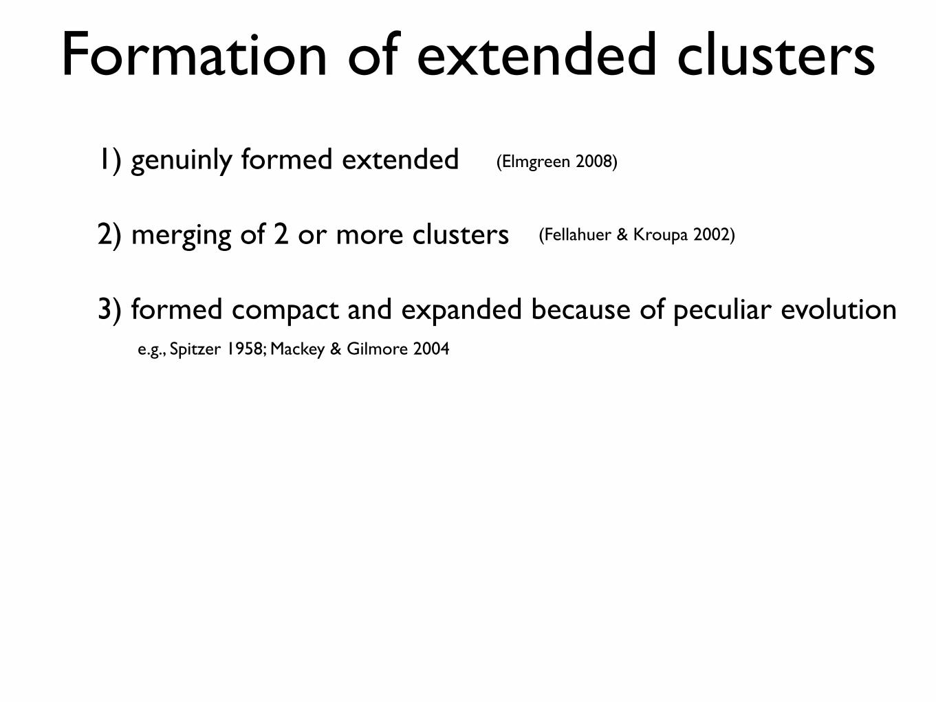
1) genuinly formed extended

2) merging of 2 or more clusters

3) formed compact and expanded because of peculiar evolution

Formation of extended clusters(Elmgreen 2008)

(Fellahuer & Kroupa 2002)

e.g., Spitzer 1958; Mackey & Gilmore 2004

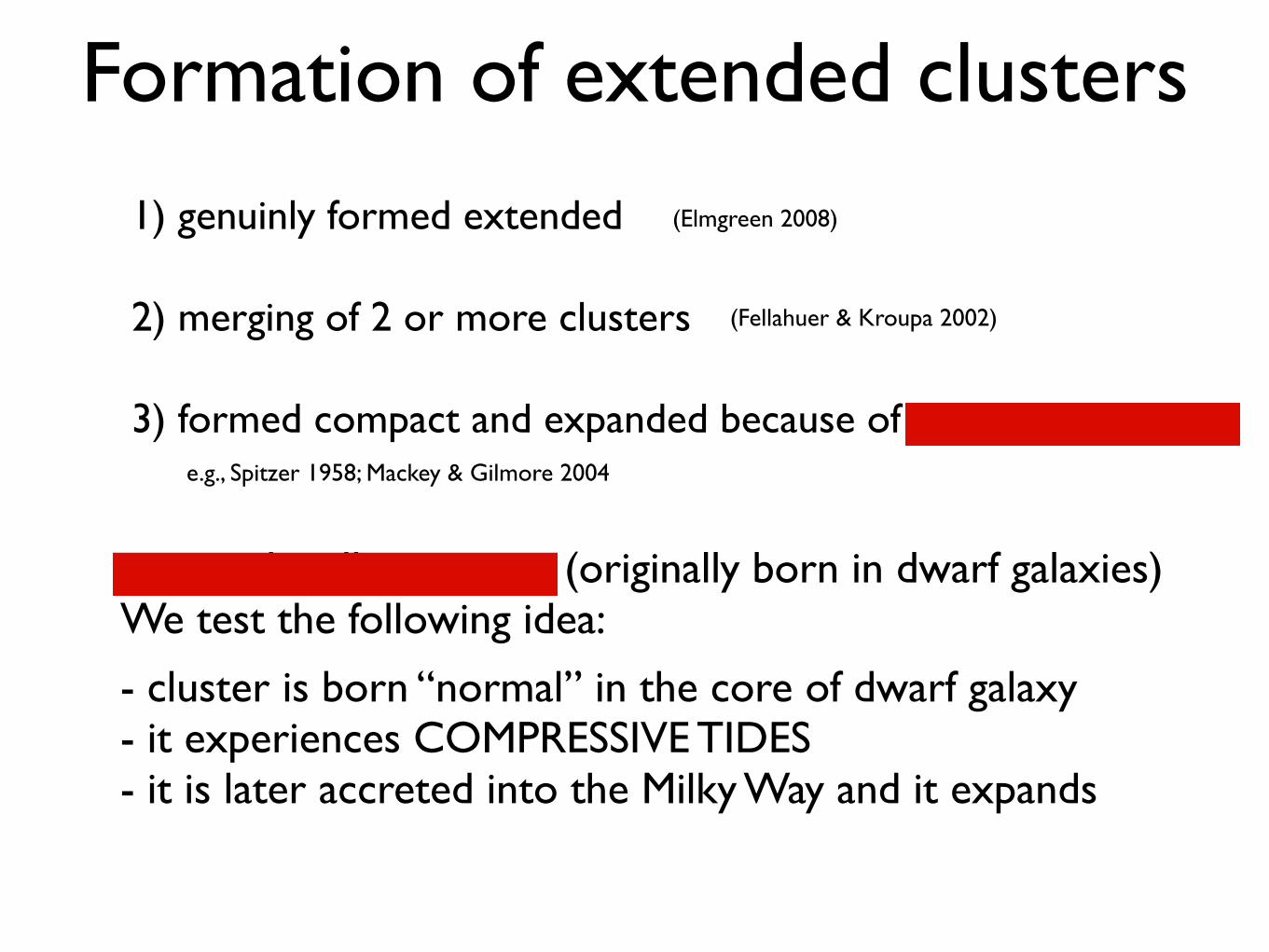
1) genuinly formed extended

2) merging of 2 or more clusters

3) formed compact and expanded because of peculiar evolution

Formation of extended clusters(Elmgreen 2008)

(Fellahuer & Kroupa 2002)

e.g., Spitzer 1958; Mackey & Gilmore 2004

accreted stellar systems (originally born in dwarf galaxies)We test the following idea:

- cluster is born “normal” in the core of dwarf galaxy- it experiences COMPRESSIVE TIDES- it is later accreted into the Milky Way and it expands

Compressive tides

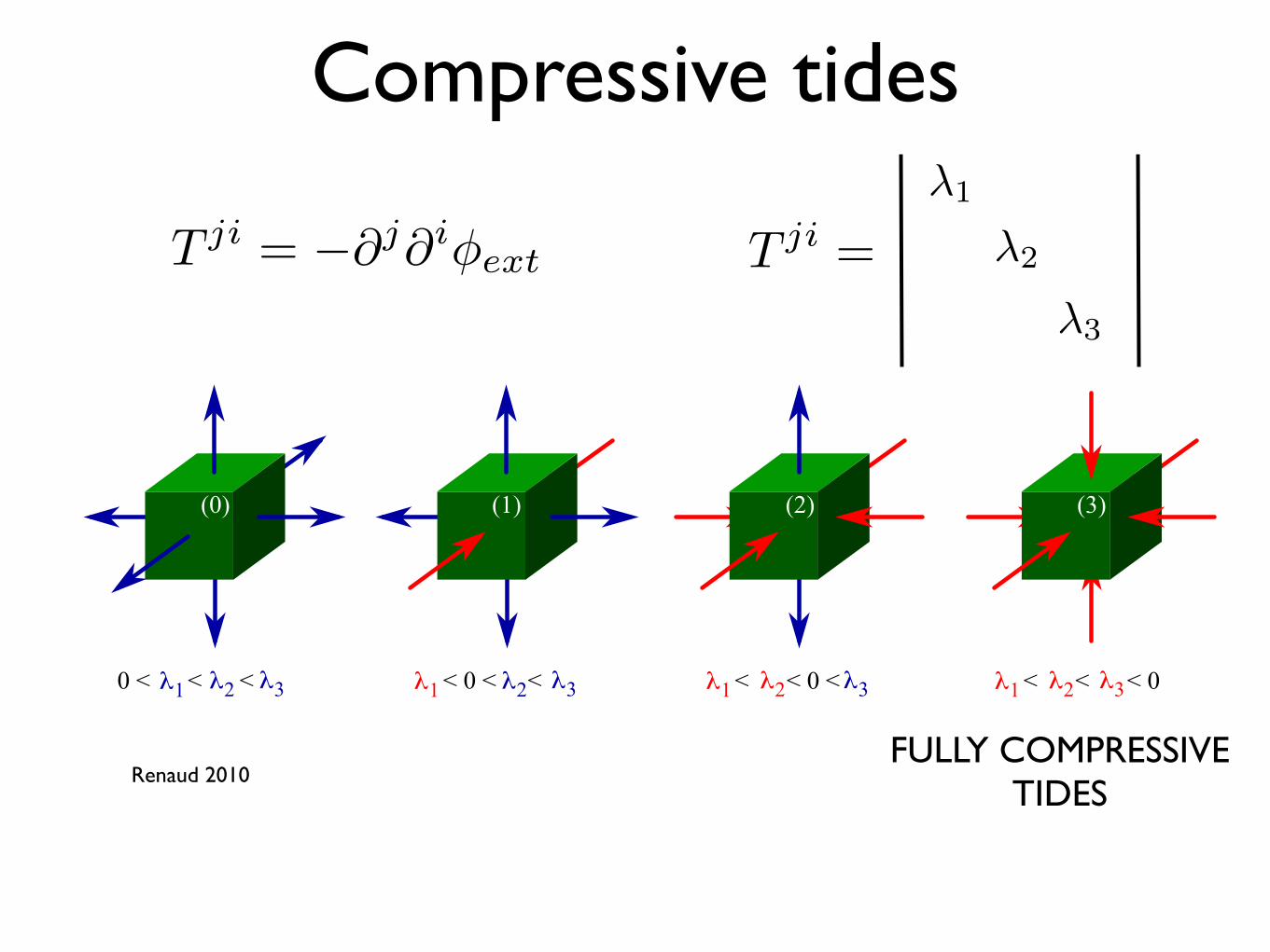
T ji = �@j@i�ext

�1

�2

�3

T ji = �@j@i�ext

General Introduction

Figure 8: Di!erent cases of tidal e!ects on an element (here, a green cube). In the con-figuration (0), all eigenvalues !i are positive and the tides act as an extensive e!ect (bluearrows). In the case (1) (respectively (2)), the tides are compressive along one (respec-tively two) direction(s) (red arrows). In the last case, the tides are fully compressive: allthe eigenvalues are negative.

2007). The last case, where all three eigenvalues are negative has been overlooked inthe literature. In this configuration, the tides are fully compressive. In the rest of thepresent manuscript, we will refer to such a case as compressive tidal mode. We will comeback to this important point in the next Chapters.

Compressive or not, the mathematical representation of the tides allows us to describethe large scale e!ects on smaller scale objects, like dwarf galaxies or star clusters.

3 Star clusters

3.1 Collection of stars

Any astronomer will tell you that clusters of galaxies contain galaxies, which containclusters of stars. Indeed, as the galaxies are often organized in clusters, the stars thatform the galaxies are themselves grouped in clusters. Discovered first during the 17thcentury, many star clusters have been catalogued by Charles Messier in 1774, withoutknowing that these objects were groups of stars. This update came later, in 1791 whenWilliam Herschel looked at M5 with his 40 feet-long telescope. He saw lots of stars inthe cluster and even a core so dense that he could not resolve all its components.

With more and more powerful observational techniques, it has been possible to detectnumerous clusters and to resolve them into stars in the Milky Way and nearby galaxies(e.g. Andromeda). Two types of clusters revealed themselves (see Figure 9):

• the globular clusters present a smooth spherical shape and a very high density in

12

Renaud 2010FULLY COMPRESSIVE

TIDES

E0 =1

2M�2 � GM2

2rv� 1

2�↵MR2

t

cluster: mass M, dispersion σ, characteristic radii Rt and rv1)

dwarf galaxy

(simple) analytical description

E0 =1

2M�2 � GM2

2rv� 1

2�↵MR2

t


2)

dwarf galaxy


compressive tides are turned off

E1 =1

2M�2 � GM2

2rv

E0 =1

2M�2 � GM2

2rv� 1

2�↵MR2

t

r0v = rv

1

1 + 2�↵R2t rv

GM

!


2)

3)

dwarf galaxy


compressive tides are turned off

E1 =1

2M�2 � GM2

2rv

system reaches new virial equilibrium

The cluster experiences a drastic change in tidal field and expands

[pc]

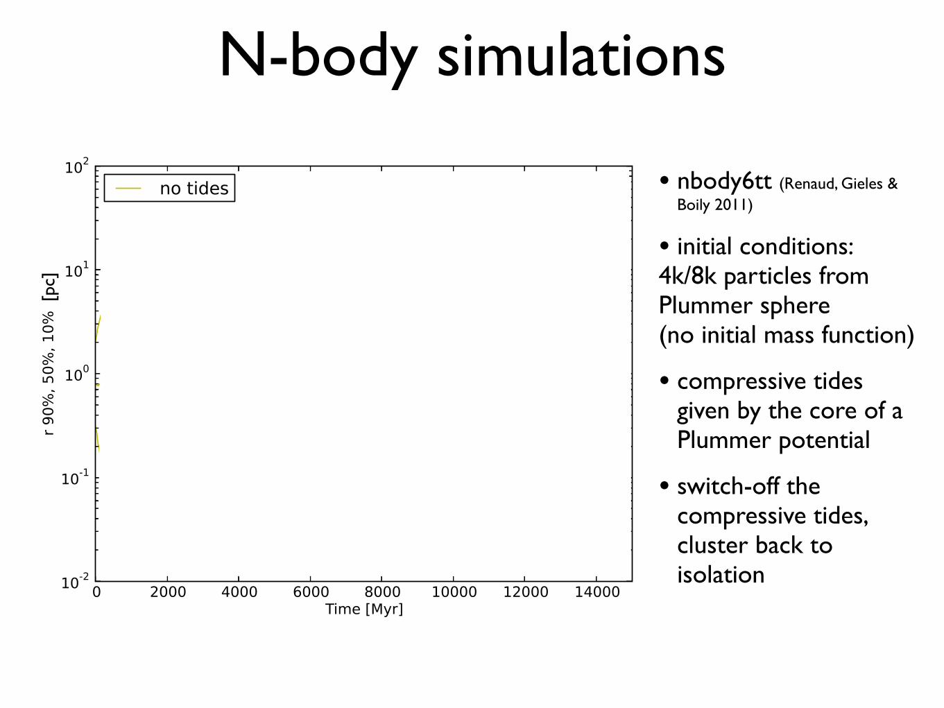
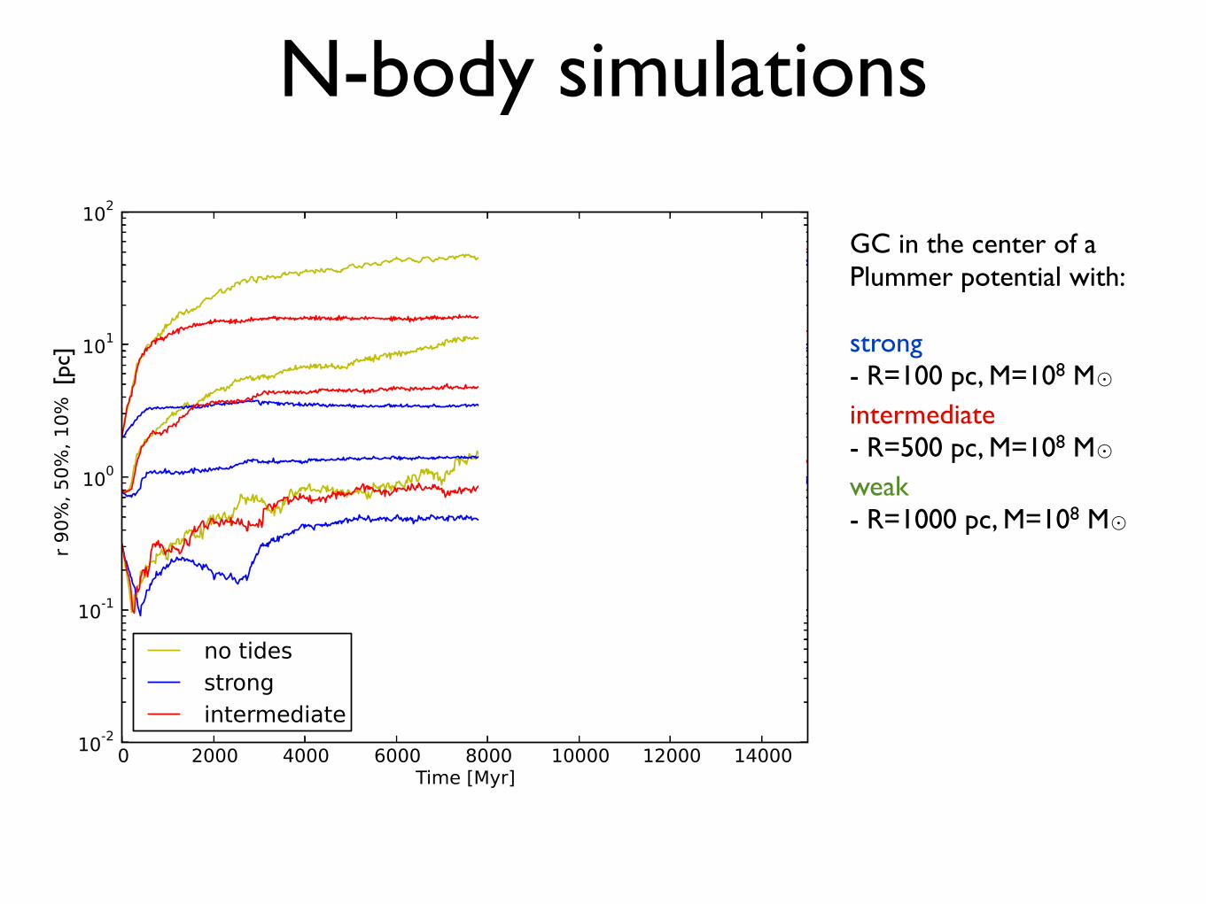
• nbody6tt (Renaud, Gieles & Boily 2011)

• initial conditions:4k/8k particles from Plummer sphere(no initial mass function)

• compressive tides given by the core of a Plummer potential

• switch-off the compressive tides, cluster back to isolation

N-body simulations

[pc]

N-body simulations

GC in the center of aPlummer potential with:

strong- R=100 pc, M=108 M�intermediate- R=500 pc, M=108 M�weak- R=1000 pc, M=108 M�

[pc]

N-body simulations

[pc]



N-body simulations

[pc]



N-body simulations

[pc]



N-body simulations

Impulsive vs. adiabatic

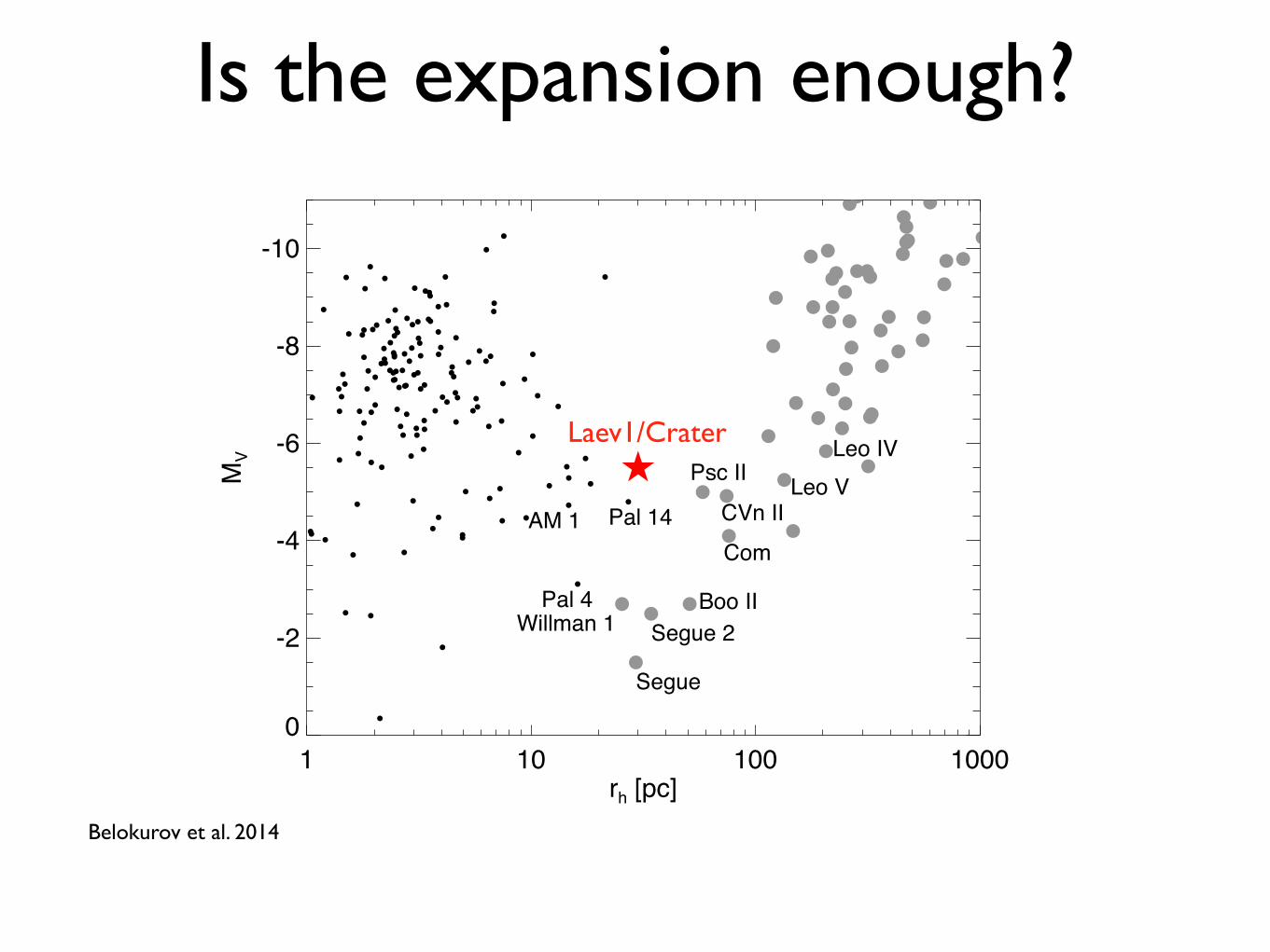
Is the expansion enough?

4 Belokurov et al.

-0.5 0.0 0.5 1.0 1.5 2.0g-i

26

24

22

20

18

16

i

-2.5-2.0 -1.5

160 350 1000m-M=21.1α/Fe=0.4

-0.5 0.0 0.5 1.0 1.5 2.0g-i

26

24

22

20

18

16

i


1 10 100 1000rh [pc]

0

-2

-4

-6

-8

-10M

V

Segue 2

Segue

Boo IIWillman 1

CVn IICom

Psc IILeo IV

Leo V

Crater

AM 1

Pal 4

Pal 14







c# 2013 RAS, MNRAS 000, 1–??

Belokurov et al. 2014

Laev1/Crater

[pc]



surface density

velocity dispersion

We DO NOT obtain clusters with density profiles more extended than the corresponding isolated case

Conclusion• we explored different initial conditions and configurations

• accreation process cannot explain extended clusters structure

• we tested an extreme case (compressive tides)

• our result is complemetary and consistent with the finding of Miholics et al. (2014)

OPEN QUESTION: how did extended clusters form?- extended clusters seem to be connected to dwarf galaxies (e.g. extended cluster found in a dwarf, Da Costa et al 2009)

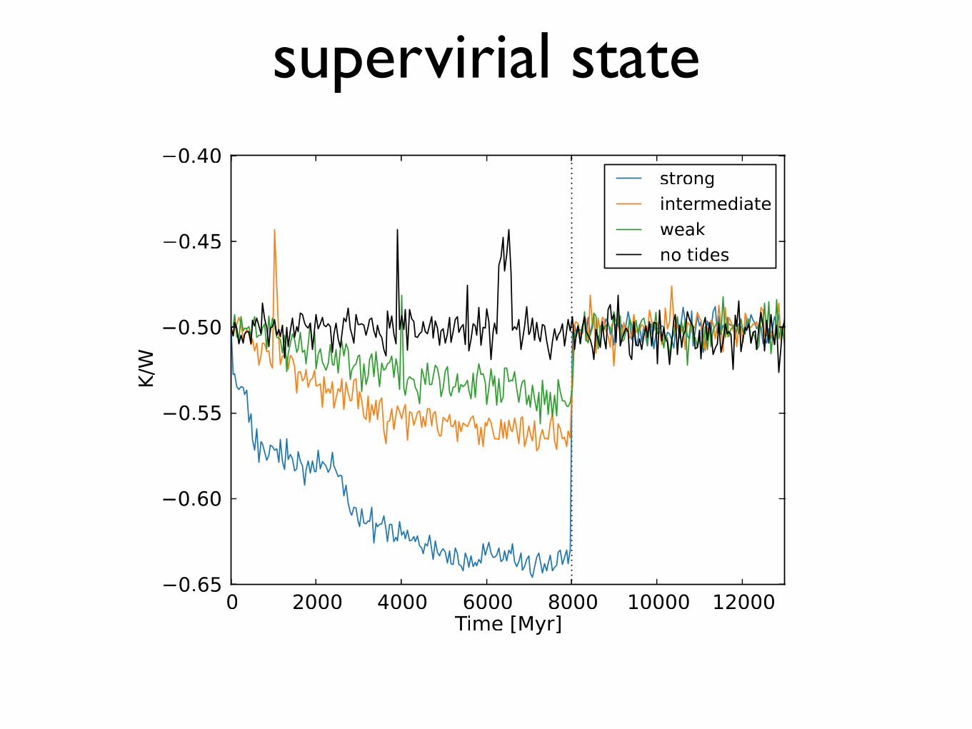
supervirial state

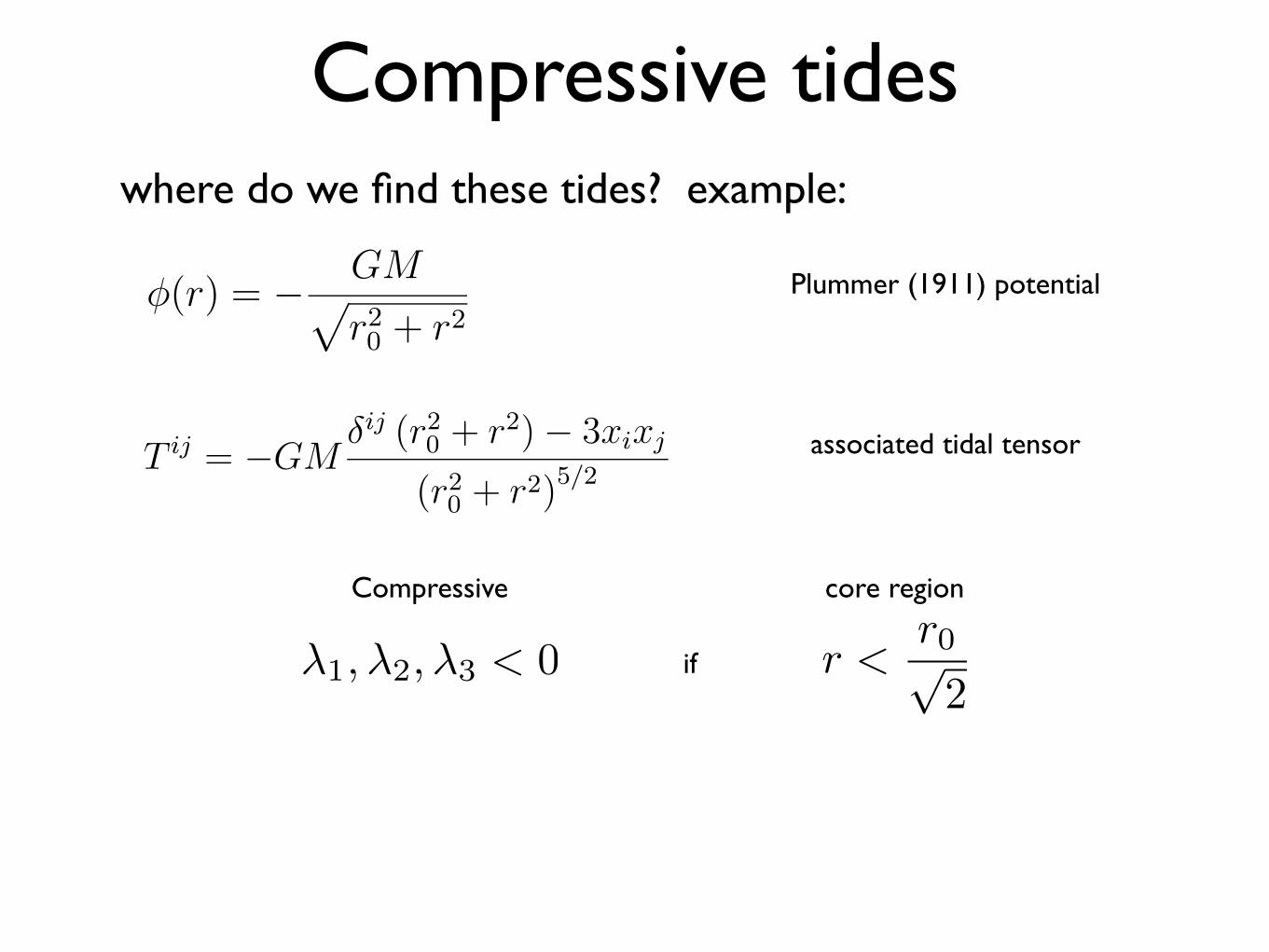
where do we find these tides? example:

Compressive tides

Appendix B

Density-potential-tidal tensortriplets

Overview

This Appendix details the analytical derivations of themain dynamical quantities of several density profiles.The notations G, !, ", T, r, M and M(r) refer to thegravitational constant, the potential, the density, thetidal tensor, the radial coordinate, the total mass, andthe mass enclosed in a sphere of radius r, respectively.

1 Classical cases

For simplicity, all the core or characteristic radii are designed by r0, while "0 representsthe characteristic density. Note however that the physical definition of these quantitiesmay vary from one model to the other, as discussed in Section V.1.4 (page 173).

1.1 Plummer

We consider the Plummer (1911) potential given by

!(r) = !GM

!

r20 + r2

. (B.1)

Using Poisson’s law (Equation A.15, page 197), we get the density

"(r) =3Mr2

0

4# (r20 + r2)5/2

. (B.2)

205

Appendix B Density-potential-tidal tensor triplets

To get the integrated mass, one can solve

M(r) = 4!

! r

0

x2"(x) dx =3M

r0

! r

0

x2

r20

"

1 + x2

r20

#5/2dx (B.3)

(which is possible through the change of variable tan # = x/r0), or simply note that thesystem must obey Newton’s second theorem

!GM(r)

r2= !"$(r), (B.4)

and get (much quicker!)

M(r) =Mr3

(r20 + r2)3/2

. (B.5)

We deduce that the radius r0 encloses # 35% of the total mass.

Starting with the potential (Equation B.1) and using Einstein’s summation conven-tion, we can derive the tidal tensor (see Equation 10, page 11):

T ij = GM%i

$

!xj

(r20 + r2)3/2

%

(B.6)

and then,

T ij = !GM&ij (r2

0 + r2) ! 3xixj

(r20 + r2)5/2

(B.7)

(with &ij = 1 if i = j and 0 otherwise), which gives, for r = x (i.e. y = z = 0):

T xx(r) = !GMr20 ! 2r2

(r20 + r2)5/2

. (B.8)

1.2 Logarithmic potential

This profile is defined by

$(r) =1

2v20 ln

&

1 +r2

r20

'

, (B.9)

where v0 denotes the circular velocity for the outer regions of the profile. The density isgiven by Poisson’s law

"(r) = v20

r2 + 3r20

(r2 + r20)

2 (B.10)

206

Plummer (1911) potential

associated tidal tensor

�1,�2,�3 < 0 r <r0p2

if

Compressive core region

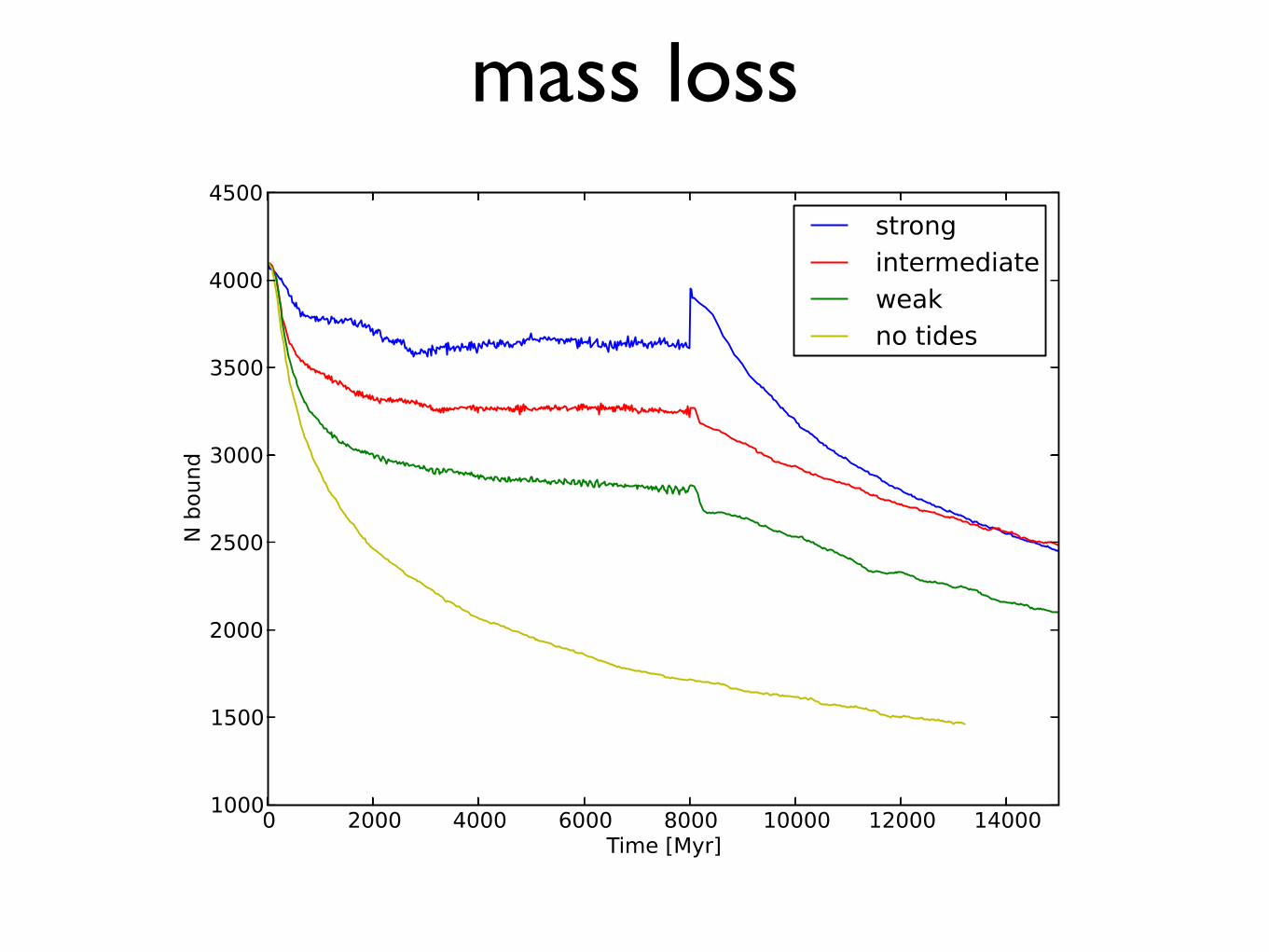
mass loss

AIMSS I 15

−5 −10 −15 −20 −25MV [mag]

1

10

100

1000

10000R

e [pc

]

EsATLAS3D

dEs/dS0s

dSphscEsAIMSS w/o m

AIMSS with mNucleiGCs/UCDs

YMCsM32

Figure 11. E↵ective radius Re vs absolute V-band magnitude MV for dynamically hot stellar systems from our master compilation.Blue stars are our observations and are filled where we have successfully measured the velocity dispersion of the object. M32 is indicatedby its own symbol and labelled. It is clear that the group of six (including one literature Coma cE) non-YMC objects with MV < –14and Re < 100pc lie o↵set significantly from the more massive previously known UCDs such as Virgo-UCD7 and Fornax-UCD3, whichare smaller than M32.

are tidally stripped from the simulations of Pfe↵er & Baum-gardt (2013). The simulations are numbers 3 (brown) and 17(orange) from Pfe↵er & Baumgardt (2013). They are bothof dE,N galaxies on elliptic orbits with apocenter of 50 kpcand pericenter of 10 kpc around a cluster centre which hasproperties chosen to match M87 in the Virgo cluster. Simu-lation 3 originally has a nucleus with Re = 4 pc and MV =–10, Simulation 17 initially has a nucleus with Re = 10 pcand MV = –12. Both are simulated for a total of 4.2 Gyr.We use these simulations to stand in for simulations of any

nucleated dwarf galaxies undergoing stripping, as at presentvery few simulations of the stripping of later type dwarfshave been carried out, but we expect that the stripping ofother dwarf galaxy types should produce reasonably simi-lar results. The simulations of Pfe↵er & Baumgardt (2013)demonstrate that the remnants of the stripping of dE,Ns canresemble almost all massive GCs and UCDs, even the mostextended (Re ⇠ 100pc) and massive (M ⇠ 108 M�) UCDssuch as Fornax-UCD3, Virgo-UCD7, and Perseus-UCD13.However, it is also clear that these simulations cannot re-

c� 2014 RAS, MNRAS 000, 1–25

Documents

Testing the formation of extended star clusters · Testing the formation of extended star clusters Paolo Bianchini (MPIA, Heidelberg) Florent Renaud, Mark Gieles & Anna Lisa Varri