Embed Size (px)
Citation preview
Testing Panel Data Regression Models with Spatial ErrorCorrelation*
by
Badi H. BaltagiDepartment of Economics, Texas A&M University,
College Station, Texas 77843-4228, USA(979) 845-7380
Seuck Heun Songand
Won KohDepartment of Statistics, Korea University,
Sungbuk-Ku, Seoul, 136-701, [email protected]
December 2001
Keywords: Panel data; Spatial error correlation, Lagrange Multiplier tests, Likelihood Ratio tests.
JEL classi…cation: C23, C12
ABSTRACT
This paper derives several Lagrange Multiplier tests for the panel data regression model wih spatialerror correlation. These tests draw upon two strands of earlier work. The …rst is the LM tests for thespatial error correlation model discussed in Anselin (1988, 1999) and Anselin, Bera, Florax and Yoon(1996), and the second is the LM tests for the error component panel data model discussed in Breuschand Pagan (1980) and Baltagi, Chang and Li (1992). The idea is to allow for both spatial errorcorrelation as well as random region e¤ects in the panel data regression model and to test for theirjoint signi…cance. Additionally, this paper derives conditional LM tests, which test for random regionale¤ects given the presence of spatial error correlation. Also, spatial error correlation given the presenceof random regional e¤ects. These conditional LM tests are an alternative to the one directional LMtests that test for random regional e¤ects ignoring the presence of spatial error correlation or the onedirectional LM tests for spatial error correlation ignoring the presence of random regional e¤ects. Weargue that these joint and conditional LM tests guard against possible misspeci…cation. ExtensiveMonte Carlo experiments are conducted to study the performance of these LM tests as well as thecorresponding Likelihood Ratio tests.
*We would like to thank the associate editor and two referees for helpful comments. An earlier version of this
paper was given at the North American Summer Meeting of the Econometric Society held at the University
of Maryland, June, 2001. Baltagi would like to thank the Bush School Program in the Economics of Public
Policy for its …nancial support.
1 INTRODUCTION
Spatial dependence models deal with spatial interaction (spatial autocorrelation) and spatial
structure (spatial heterogeneity) primarily in cross-section data, see Anselin (1988, 1999).
Spatial dependence models use a metric of economic distance, see Anselin (1988) and Conley
(1999) to mention a few. This measure of economic distance provides cross-sectional data with
a structure similar to that provided by the time index in time series. There is an extensive
literature estimating these spatial models using maximum likelihood methods, see Anselin
(1988). More recently, generalized method of moments have been proposed by Kelejian and
Prucha (1999) and Conley (1999). Testing for spatial dependence is also extensively studied
by Anselin (1988, 1999), Anselin and Bera (1998), Anselin, Bera, Florax and Yoon (1996) to
mention a few.
With the increasing availability of micro as well as macro level panel data, spatial panel data
models studied in Anselin (1988) are becoming increasingly attractive in empirical economic
research. See Case (1991), Kelejian and Robinson (1992), Case, Hines and Rosen (1993),
Holtz-Eakin (1994), Driscoll and Kraay (1998), Baltagi and Li (1999) and Bell and Bockstael
(2000) for a few applications. Convergence in growth models that use a pooled set of countries
over time could have spatial correlation as well as heterogeneity across countries to contend
with, see Delong and Summers (1991) and Islam (1995) to mention a few studies. County
level data over time, whether it is expenditures on police, or measuring air pollution levels can
be treated with these models. Also, state level expenditures over time on welfare bene…ts,
mass transit, etc. Household level survey data from villages observed over time to study
nutrition, female labor participation rates, or the e¤ects of education on wages could exhibit
spatial correlation as well as heterogeneity across households and this can be modeled with
a spatial error component model.
Estimation and testing using panel data models have also been extensively studied, see Hsiao
(1986) and Baltagi (2001), but these models ignore the spatial correlation. Heterogeneity
across the cross-sectional units is usually modeled with an error component model. A La-
grange multiplier test for random e¤ects was derived by Breusch and Pagan (1980), and an
extensive Monte Carlo on testing in this error component model was performed by Baltagi,
Chang and Li (1992). This paper extends the Breusch and Pagan LM test to the spatial
error component model. First, a joint LM test is derived which simultaneously tests for the
existence of spatial error correlation as well as random region e¤ects. This LM test is based
on the estimation of the model under the null hypothesis and its computation is simple requir-
ing only least squares residuals. This test is important, because ignoring spatial correlation
and heterogeneity due to the random region e¤ects will result in ine¢cient estimates and
1
misleading inference. Next, two conditional LM tests are derived. One for the existence of
spatial error correlation assuming the presence of random region e¤ects, and the other for the
existence of random region e¤ects assuming the presence of spatial error correlation. These
tests guard against misleading inference caused by (i) one directional LM tests that ignore
the presence of random region e¤ects when testing for spatial error correlation, or (ii) one
directional LM tests that ignore the presence of spatial correlation when testing for random
region e¤ects.
Section 2 revisits the spatial error component model considered in Anselin (1988) and provides
the joint and conditional LM tests proposed in this paper. Only the …nal LM test statistics
are given in the paper. Their derivations are relegated to the Appendices. Section 3 compares
the performance of these LM tests as well as the corresponding likelihood ratio LR tests using
Monte Carlo experiments. Section 4 gives a summary and conclusion.
2 THE MODEL AND TEST STATISTICS
Consider the following panel data regression model, see Baltagi (2001):
yti = X 0ti¯ + uti; i = 1; ::; N ; t = 1; ¢ ¢ ¢ ; T; (2.1)
where yti is the observation on the ith region for the tth time period, Xti denotes the kx1
vector of observations on the non-stochastic regressors and uti is the regression disturbance.
In vector form, the disturbance vector of (2.1) is assumed to have random region e¤ects as
well as spatially autocorrelated residual disturbances, see Anselin (1988):
ut = ¹ + ²t; (2.2)
with
²t = ¸W²t + ºt; (2.3)
where u0t = (ut1; : : : ; utN), ²0t = (²t1; : : : ; ²tN ) and ¹0 = (¹1; ¢ ¢ ¢ ; ¹N) denote the vector of
random region e¤ects which are assumed to be IIN(0; ¾2¹): ¸ is the scalar spatial autoregres-
sive coe¢cient with j ¸ j< 1: W is a known N £ N spatial weight matrix whose diagonal
elements are zero. W also satis…es the condition that (IN¡¸W ) is nonsingular for all j ¸ j< 1.
º0t = (ºt1; ¢ ¢ ¢ ; ºtN ); where ºti is i:i:d: over i and t and is assumed to be N(0; ¾2º): The fºtig
process is also independent of the process f¹ig. One can rewrite (2.3) as
²t = (IN ¡ ¸W )¡1ºt = B¡1ºt; (2.4)
2
where B = IN ¡ ¸W and IN is an identity matrix of dimension N . The model (2.1) can be
rewritten in matrix notation as
y = X¯ + u; (2.5)
where y is now of dimension NT £ 1, X is NT £ k, ¯ is k £ 1 and u is NT £ 1: The
observations are ordered with t being the slow running index and i the fast running index,
i.e., y0 = (y11; : : : ; y1N ; : : : ; yT1; : : : ; yTN): X is assumed to be of full column rank and its
elements are assumed to be asymptotically bounded in absolute value. Equation (2.2) can
be written in vector form as:
u = (¶T IN )¹ + (IT B¡1)º; (2.6)
where º0 = (º01; ¢ ¢ ¢ ; º0T ), ¶T is a vector of ones of dimension T , IT is an identity matrix of
dimension T and denotes the Kronecker product. Under these assumptions, the variance-
covariance matrix for u can be written as
u = ¾2¹(JT IN) + ¾2
º(IT (B0B)¡1); (2.7)
where JT is a matrix of ones of dimension T . This variance-covariance matrix can be rewritten
as:
u = ¾2º
h¹JT (TÁIN + (B0B)¡1) + ET (B0B)¡1
i= ¾2
º§u; (2.8)
where Á = ¾2¹=¾2
º , ¹JT = JT=T; ET = IT ¡ ¹JT and §u =h
¹JT (TÁIN + (B0B)¡1) + ET (B0B)¡1
i: Using results in Wansbeek and Kapteyn (1983), §¡1u is given by
§¡1u = ¹JT (TÁIN + (B0B)¡1)¡1 + ET B0B: (2.9)
Also, j§uj = jTÁIN + (B0B)¡1j ¢ j(B0B)¡1jT¡1: Under the assumption of normality, the log-
likelihood function for this model was derived by Anselin (1988, p.154) as
L = ¡NT2
ln 2¼¾2º ¡ 1
2ln j§uj ¡
12¾2ºu0§¡1u u
= ¡NT2
ln 2¼¾2º ¡ 1
2ln[jTÁIN + (B0B)¡1j] +
(T ¡ 1)2
ln jB0Bj
¡ 12¾2ºu0§¡1u u; (2.10)
with u = y ¡ X¯. Anselin (1988, p.154) derived the LM test for ¸ = 0 in this model. Here,
we extend Anselin’s work by deriving the joint test for spatial error correlation as well as
random region e¤ects.
The hypotheses under consideration in this paper are the following:
3

(a) Ha0 : ¸ = ¾2¹ = 0, and the alternative Ha1 is that at least one component is not zero.
(b) Hb0 : ¾2¹ = 0 (assuming no spatial correlation, i.e., ¸ = 0), and the one-sided alternative
Hb1 is that ¾2¹ > 0 (assuming ¸ = 0).
(c) Hc0 : ¸ = 0 (assuming no random e¤ects, i.e., ¾2¹ = 0), and the two-sided alternative is
Hc1 : ¸ 6= 0 (assuming ¾2¹ = 0).
(d) Hd0 : ¸ = 0 (assuming the possible existence of random e¤ects, i.e., ¾2¹ ¸ 0), and the
two-sided alternative is Hd1 : ¸ 6= 0 (assuming ¾2¹ ¸ 0).
(e) He0 : ¾2¹ = 0 (assuming the possible existence of spatial correlation, i.e., ¸ may be zero
or di¤erent from zero), and the one-sided alternative is He1 : ¾2¹ > 0 (assuming that ¸
may be zero or di¤erent from zero).
In the next sections, we derive the corresponding LM tests for these hypotheses and we
compare their performance with the corresponding LR tests using Monte Carlo experiments.
2.1 Joint LM Test for Ha0: ¸ = ¾2¹ = 0
The joint LM test statistic for testing Ha0 : ¸ = ¾2¹ = 0 vs Ha1 is given by
LMJ =NT
2(T ¡ 1)G2 +
N2Tb
H2; (2.11)
where G = ~u0(JTIN )~u~u0~u ¡ 1, H = ~u0(ITW )~u
~u0~u , b = tr(W + W 0)2=2 = tr(W 2 + W 0W ) and ~u
denotes the OLS residuals. The derivation of this LM test statistic is given in Appendix A.1.
It is important to note that the large sample distribution of the LM test statistics derived
in this paper are not formally established, but are likely to hold under similar sets of low
level assumptions developed in Kelejian and Prucha (2001) for the Moran I test statistic
and its close cousins the LM tests for spatial correlation. See also Pinkse (1998, 1999) for
general conditions under which Moran ‡avoured tests for spatial correlation have a limiting
normal distribution in the presence of nuisance parameters in six frequently encountered
spatial models. Section 2.4 shows that the one-sided version of this joint LM test should be
used because variance components cannot be negative
2.2 Marginal LM Test for Hb0: ¾2¹ = 0 (assuming ¸ = 0)
Note that the …rst term in (2.11), call it LMG = NT2(T¡1)G
2; is the basis for the LM test statistic
for testing Hb0 : ¾2¹ = 0 assuming there are no spatial error dependence e¤ects, i.e., assuming
4

that ¸ = 0, see Breusch and Pagan (1980). This LM statistic should be asymptotically
distributed as Â21 under Hb0 as N ! 1; for a given T . But this LM test has the problem
that the alternative hypothesis is assumed to be two-sided when we know that the variance
component cannot be negative. Honda (1985) suggested a uniformly most powerful test for
Hb0 based upon the square root of the G2 term, i.e.,
LM1 =
sNT
2(T ¡ 1)G: (2.12)
This should be asymptotically distributed as N(0,1) under Hb0 as N ! 1; for T …xed.
Moulton and Randolph(1989) showed that the asymptotic N(0,1) approximation for this
one sided LM test can be poor even in large samples. This occurs when the number of
regressors is large or the intra-class correlation of some of the regressors is high. They
suggest an alternative standardized LM (SLM) test statistic whose asymptotic critical values
are generally closer to the exact critical values than those of the LM test. This SLM test
statistic centers and scales the one sided LM statistic so that its mean is zero and its variance
is one:
SLM1 =LM1 ¡ E(LM1)p
var(LM1)=
d1 ¡ E(d1)pvar(d1)
; (2.13)
where d1 =~u0D1~u~u0~u
and D1 = (JT IN) with ~u denoting the OLS residuals. Using the
normality assumption and results on moments of quadratic forms in regression residuals (see
e.g. Evans and King, 1985), we get
E(d1) = tr(D1M)=s; (2.14)
where s = NT ¡ k and M = INT ¡ X(X 0X)¡1X 0. Also.
var(d1) = 2fs tr(D1M)2 ¡ [tr(D1M)]2g=s2(s + 2): (2.15)
Under Hb0; SLM1 should be asymptotically distributed as N(0,1).
2.3 Marginal LM Test for Hc0: ¸ = 0 (assuming ¾2¹ = 0)
Similarly, the second term in (2.11), call it LMH = N2Tb H2; is the basis for the LM test
statistic for testing Hc0: ¸ = 0 assuming there are no random regional e¤ects, i.e., assuming
that ¾2¹ = 0, see Anselin (1988). This LM statistic should be asymptotically distributed as
Â21 under Hc0. Alternatively, this can be obtained as
LM2 =
rN2T
bH: (2.16)
5

This LM2 test statistic should be asymptotically distributed as N(0; 1) under Hc0. The
corresponding standardized LM (SLM) test statistic is given by
SLM2 =LM2 ¡ E(LM2)p
var(LM2)=
d2 ¡ E(d2)pvar(d2)
; (2.17)
where d2 =~u0D2~u~u0~u
and D2 = (IT W ). Under Hc0; SLM2 should be asymptotically distrib-
uted as N(0; 1). SLM2 should have asymptotic critical values that are generally closer to the
corresponding exact critical values than those of the unstandardized LM2 test statistic.
2.4 One-Sided Joint LM Test for Ha0 : ¸ = ¾2¹ = 0
Following Honda (1985) for the two-way error component model, a handy one-sided test
statistic for Ha0 : ¸ = ¾2¹ = 0 is given by
LMH = (LM1 + LM2)=p
2; (2.18)
which is asymptotically distributed N(0; 1) under Ha0 .
Note that LM1 in (2.12) can be negative for a speci…c application, especially when the true
variance component ¾2¹ is small and close to zero. Similarly, LM2 in (2.16) can be negative
especially when the true ¸ is small and close to zero. Following Gourieroux, Holly and
Monfort (1982), here after GHM, we propose the following test for the joint null hypothesis
Ha0 :
Â2m =
8>>>>>>><>>>>>>>:
LM21 + LM2
2 if LM1 > 0; LM2 > 0
LM21 if LM1 > 0; LM2 · 0
LM22 if LM1 · 0; LM2 > 0
0 if LM1 · 0; LM2 · 0 ;
(2.19)
Under the null hypothesis Ha0 , Â2m has a mixed Â2- distribution:
Â2m » (
14)Â2(0) + (
12)Â2(1) + (
14)Â2(2); (2.20)
where Â2(0) equals zero with probability one. The weights (14); (12) and (14) follow from the
fact that LM1 and LM2 are asymptotically independent of each other and the results in
Gourieroux, Holly and Monfort (1982). The critical values for the mixed Â2m are 7:289, 4:321
and 2:952 for ® = 0:01, 0:05 and 0:1, respectively.
6

2.5 LR Test for Ha0 : ¸ = ¾2¹ = 0
We also compute the Likelihood ratio (LR) test for Ha0 : ¸ = ¾2¹ = 0. Estimation of the
unrestricted log-likelihood function is obtained using the method of scoring. The details of
the estimation procedure are available upon request from the authors. Let b¾2º , bÁ, b and b
denote the unrestricted maximum likelihood estimators and let bB = IN¡bW and bu = y¡X 0b,
then the unrestricted maximum log-likelihood estimator function is given by
LU = ¡NT2
ln 2¼¾2º ¡ 1
2ln[jTbÁIN + ( bB0 bB)¡1j] + (T ¡ 1) ln j bBj ¡ 1
2b¾2ºu0b§¡1u u; (2.21)
see Anselin (1988), where b§ is obtained from (2.8) with bB replacing B and bÁ replacing Á: But
under the null hypothesis Ha0 , the variance-covariance matrix reduces to ¤u = u = ¾2ºITN
and the restricted maximum likelihood estimator of ¯ is ~OLS , so that ~u = y ¡ X 0 ~
OLS
are the OLS residuals and ~¾2º = ~u0~u=NT . Therefore, the restricted maximum log-likelihood
function under Ha0 is given by
LR = ¡NT2
ln 2¼~¾2º ¡ 1
2~¾2º~u0~u: (2.22)
Hence, the likelihood ratio test statistic for Ha0 : ¸ = ¾2¹ = 0 is given by
LR¤J = 2(LU ¡ LR); (2.23)
and this should be asymptotically distributed as a mixture of Â2 given in (2.20) under the
null hypothesis.
2.6 Conditional LM Test for Hd0 : ¸ = 0 (assuming ¾2¹ ¸ 0)
When one uses LM2; given by (2.16), to test Hc0 : ¸ = 0; one implicitly assumes that the
random region e¤ects do not exist. This may lead to incorrect decisions especially when ¾2¹
is large. To overcome this problem, this section derives a conditional LM test for spatially
uncorrelated disturbances assuming the possible existence of random regional e¤ects. The
null hypothesis for this model is Hd0 : ¸ = 0 (assuming ¾2¹ ¸ 0). Under the null hyphothesis,
the variance-covariance matrix reduces to 0 = ¾2¹JT IN + ¾2
ºINT . It is the familiar form
of the one-way error component model, see Baltagi(1995), with ¡10 = (¾21)¡1( ¹JT IN) +
(¾2º)¡1(ET IN), where ¾2
1 = T¾2¹ + ¾2
º ; and ET = IT ¡ ¹JT . Using derivations analogous
to those for the joint LM-test, see Appendix A.1, we obtain the following LM test for Hd0 vs
Hd1 ,
7
LM¸ =D(¸)2
[(T ¡ 1) + ¾4º¾41
]b, (2.24)
where
D(¸) =12u0[
¾2º
¾41( ¹JT (W 0 + W )) +
1¾2º(ET (W 0 + W ))]u:
Here, ¾2º = u0(ET IN )u=N(T ¡ 1) and ¾2
1 = u0( ¹JT IN)u=N are the maximum likelihood
estimates of ¾2º and ¾2
1 under Hd0 , and u denotes the maximum likelihood residuals under the
null hypothesis Hd0 . See Appendix A.2 for more details.
Therefore, the one-sided test for zero spatial error dependence (assuming ¾2¹ ¸ 0) against an
alternative, say of ¸ > 0 is obtained from
LM¤¸ =
D(¸)r[(T ¡ 1) + ¾4º
¾41]b
; (2.25)
and this test statistic should be asymptotically distributed as N(0; 1) under Hd0 for N ! 1and T …xed.
We can also get the LR test for Hd0 , using the scoring method. Details are available upon
request from the authors. Under the null hypothesis, the LR test statistic will have the same
asymptotic distribution as its LM counterpart.
2.7 Conditional LM Test for He0: ¾2¹ = 0 (assuming ¸ may or may not be= 0)
Similarly, if one uses LM1; given by (2.12), to test Hb0 : ¾2¹ = 0; one is implicitly assuming
that no spatial error correlation exists. This may lead to incorrect decisions especially when
¸ is signi…cantly di¤erent from zero. To overcome this problem, this section derives a condi-
tional LM test for no random regional e¤ects assuming the possible existence of spatial error
correlation. The null hypothesis for this model is He0 : ¾2¹ = 0 (assuming ¸ may or may not
be = 0).
This LM test statistic is derived in Appendix A.3 and is given by
LM¹ = D0¹ J¡1µ D¹; (2.26)
where
D¹ = ¡ T2b¾2ºtr( bB0 bB) +
12b¾4ºbu0[JT ( bB0 bB)2]bu; (2.27)
8
and
bJµ =
2664
TN2b¾2º
NT2b¾2º
tr[(W 0 bB + bB0W ) + ( bB0 bB)¡1] T2b¾4º
tr[ bB0 bB]T2 tr
£¡(W 0 bB + bB0W ) + ( bB0 bB)¡1
¢2¤ T2b¾2º
tr[W 0 bB + bB0W ]T 22b¾4º
tr[( bB0 bB)2]
3775 ; (2.28)
=T
2¾4º
24
N ¾2ºg h
¾2ºg ¾4
º c ¾2º d
h ¾2º d Te
35 : (2.29)
where g = tr[(W 0 bB + bB0W )( bB0 bB)¡1], h = tr[ bB0 bB], c = tr·³
(W 0 bB + bB0W )( bB0 bB)¡1´2
¸, d =
tr[W 0 bB + bB0W ] and e = tr[( bB0 bB)2]. Therefore,
LM¹ = (D¹)2³2¾4
ºT
´³TN¾4
ºec ¡ N¾4ºd
2 ¡ T¾4ºg
2e + 2¾4ºghd ¡ ¾4
ºh2c
´¡1
³N¾4ºc ¡ ¾4
ºg2´: (2.30)
where bD¹ and bJµ are evaluated at the maximum likelihood estimates under the null hypoth-
esis He0 . However, LM¹ ignores the fact that the variance component cannot be negative.
Therefore, the one-sided version of this LM test is given by
LM¤¹ =
D¹q
(2¾4º=T )(N¾4
ºc ¡ ¾4ºg2)q
TN¾4ºec ¡ N¾4
ºd2 ¡ T ¾4ºg2e + 2¾4
ºghd ¡ ¾4ºh2c
(2.31)
and this should be asymptotically distributed as N(0; 1) under He0 as N ! 1 for T …xed.
3 MONTE CARLO RESULTS
The experimental design for the Monte Carlo simulations is based on the format extensively
used in earlier studies in the spatial regression model by Anselin and Rey (1991) and Anselin
and Florax (1995) and in the panel data model by Nerlove (1971).
The model is set as follows :
yit = ® + x0it¯ + uit; i = 1; ¢ ¢ ¢ N; t = 1; ¢ ¢ ¢ ; T; (3.1)
where ® = 5 and ¯ = 0:5. xit is generated by a similar method to that of Nerlove (1971). In
fact, xit = 0:1t+0:5xi;t¡1+zit, where zit is uniformly distributed over the interval [¡0:5; 0:5].
The initial values xi0 are chosen as (5 + 10zi0). For the disturbances, uit = ¹i + "it, "it =
¸PNj=1 wij"it + ºit with ¹i » IIN(0; ¾2
¹) and ºit » IIN(0; ¾2º): The matrix W is either a
9
rook or a queen type weight matrix, and the rows of this matrix are standardized so that they
sum to one.1 We …x ¾2¹+¾2
º = 20 and let ½ = ¾2¹=(¾2
¹+¾2º) vary over the set (0; 0:2; 0:5; 0:8).
The spatial autocorrelation factor ¸ is varied over a positive range from 0 to 0:9 by increments
of 0:1. Two values for N = 25 and 49, and two values for T = 3 and 7 are chosen. In total,
this amounts to 320 experiments.2 For each experiment, the joint, conditional and marginal
LM and LR tests are computed and 2000 replications are performed. In a …rst draft of this
paper we reported the two-sided LM and LR test results to show how misleading the results
of these tests can be. These results are available upon request from the authors. In this
version, we focus on the one-sided version of these tests except for testing Hb0: ¾2¹ = 0 where
we thought a warning should be given to applied econometricans using packages that still
report two-sided versions of this test.
3.1 Joint Tests for Ha0 : ¸ = ¾2¹ = 0
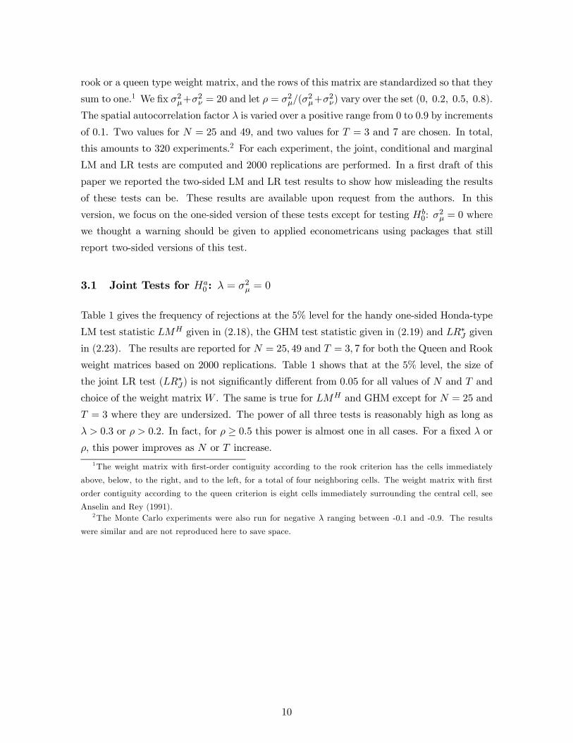
Table 1 gives the frequency of rejections at the 5% level for the handy one-sided Honda-type
LM test statistic LMH given in (2.18), the GHM test statistic given in (2.19) and LR¤J given
in (2.23). The results are reported for N = 25; 49 and T = 3; 7 for both the Queen and Rook
weight matrices based on 2000 replications. Table 1 shows that at the 5% level, the size of
the joint LR test (LR¤J) is not signi…cantly di¤erent from 0:05 for all values of N and T and
choice of the weight matrix W . The same is true for LMH and GHM except for N = 25 and
T = 3 where they are undersized. The power of all three tests is reasonably high as long as
¸ > 0:3 or ½ > 0:2. In fact, for ½ ¸ 0:5 this power is almost one in all cases. For a …xed ¸ or
½, this power improves as N or T increase.1The weight matrix with …rst-order contiguity according to the rook criterion has the cells immediately
above, below, to the right, and to the left, for a total of four neighboring cells. The weight matrix with …rst
order contiguity according to the queen criterion is eight cells immediately surrounding the central cell, see
Anselin and Rey (1991).2The Monte Carlo experiments were also run for negative ¸ ranging between -0.1 and -0.9. The results
were similar and are not reproduced here to save space.
10
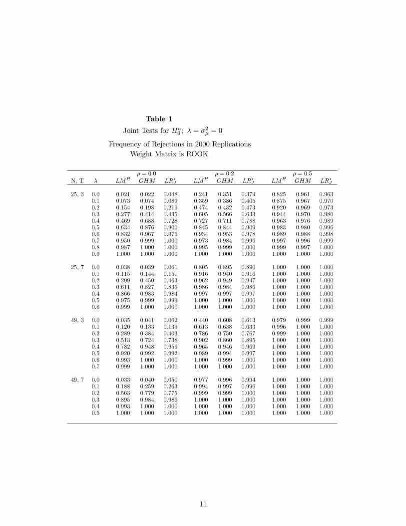
Table 1Joint Tests for Ha0 ; ¸ = ¾2
¹ = 0
Frequency of Rejections in 2000 ReplicationsWeight Matrix is ROOK
½ = 0:0 ½ = 0:2 ½ = 0:5N, T ¸ LMH GHM LR¤J LMH GHM LR¤J LMH GHM LR¤J
25, 3 0.0 0.021 0.022 0.048 0.241 0.351 0.379 0.825 0.961 0.9630.1 0.073 0.074 0.089 0.359 0.386 0.405 0.875 0.967 0.9700.2 0.154 0.198 0.219 0.474 0.432 0.473 0.920 0.969 0.9730.3 0.277 0.414 0.435 0.605 0.566 0.633 0.944 0.970 0.9800.4 0.469 0.688 0.728 0.727 0.711 0.788 0.963 0.976 0.9890.5 0.634 0.876 0.900 0.845 0.844 0.909 0.983 0.980 0.9960.6 0.832 0.967 0.976 0.934 0.953 0.978 0.989 0.988 0.9980.7 0.950 0.999 1.000 0.973 0.984 0.996 0.997 0.996 0.9990.8 0.987 1.000 1.000 0.995 0.999 1.000 0.999 0.997 1.0000.9 1.000 1.000 1.000 1.000 1.000 1.000 1.000 1.000 1.000
25, 7 0.0 0.038 0.039 0.061 0.805 0.895 0.890 1.000 1.000 1.0000.1 0.115 0.144 0.151 0.916 0.940 0.916 1.000 1.000 1.0000.2 0.299 0.450 0.463 0.962 0.949 0.947 1.000 1.000 1.0000.3 0.611 0.827 0.836 0.986 0.984 0.986 1.000 1.000 1.0000.4 0.866 0.983 0.984 0.997 0.997 0.997 1.000 1.000 1.0000.5 0.975 0.999 0.999 1.000 1.000 1.000 1.000 1.000 1.0000.6 0.999 1.000 1.000 1.000 1.000 1.000 1.000 1.000 1.000
49, 3 0.0 0.035 0.041 0.062 0.440 0.608 0.613 0.979 0.999 0.9990.1 0.120 0.133 0.135 0.613 0.638 0.633 0.996 1.000 1.0000.2 0.289 0.384 0.403 0.786 0.750 0.767 0.999 1.000 1.0000.3 0.513 0.724 0.738 0.902 0.860 0.895 1.000 1.000 1.0000.4 0.782 0.948 0.956 0.965 0.946 0.969 1.000 1.000 1.0000.5 0.920 0.992 0.992 0.989 0.994 0.997 1.000 1.000 1.0000.6 0.993 1.000 1.000 1.000 0.999 1.000 1.000 1.000 1.0000.7 0.999 1.000 1.000 1.000 1.000 1.000 1.000 1.000 1.000
49, 7 0.0 0.033 0.040 0.050 0.977 0.996 0.994 1.000 1.000 1.0000.1 0.188 0.259 0.263 0.994 0.997 0.996 1.000 1.000 1.0000.2 0.563 0.779 0.775 0.999 0.999 1.000 1.000 1.000 1.0000.3 0.895 0.984 0.986 1.000 1.000 1.000 1.000 1.000 1.0000.4 0.993 1.000 1.000 1.000 1.000 1.000 1.000 1.000 1.0000.5 1.000 1.000 1.000 1.000 1.000 1.000 1.000 1.000 1.000
11
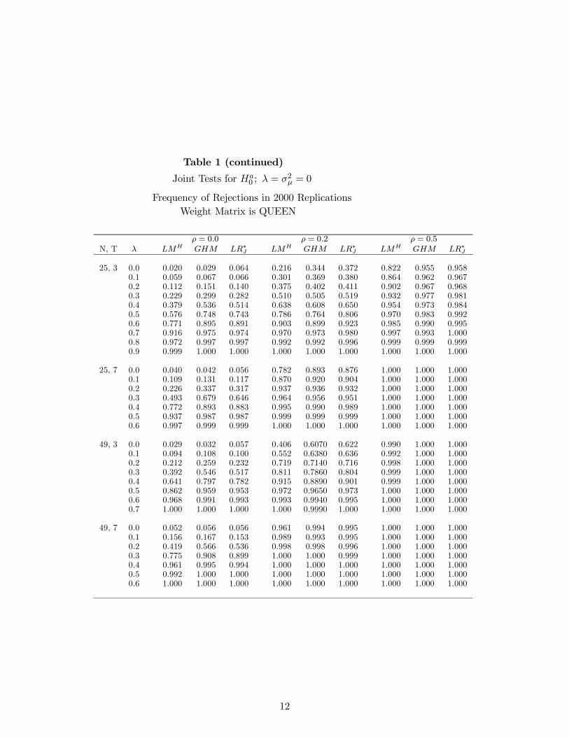
Table 1 (continued)Joint Tests for Ha0 ; ¸ = ¾2
¹ = 0
Frequency of Rejections in 2000 ReplicationsWeight Matrix is QUEEN
½ = 0:0 ½ = 0:2 ½ = 0:5N, T ¸ LMH GHM LR¤J LMH GHM LR¤J LMH GHM LR¤J
25, 3 0.0 0.020 0.029 0.064 0.216 0.344 0.372 0.822 0.955 0.9580.1 0.059 0.067 0.066 0.301 0.369 0.380 0.864 0.962 0.9670.2 0.112 0.151 0.140 0.375 0.402 0.411 0.902 0.967 0.9680.3 0.229 0.299 0.282 0.510 0.505 0.519 0.932 0.977 0.9810.4 0.379 0.536 0.514 0.638 0.608 0.650 0.954 0.973 0.9840.5 0.576 0.748 0.743 0.786 0.764 0.806 0.970 0.983 0.9920.6 0.771 0.895 0.891 0.903 0.899 0.923 0.985 0.990 0.9950.7 0.916 0.975 0.974 0.970 0.973 0.980 0.997 0.993 1.0000.8 0.972 0.997 0.997 0.992 0.992 0.996 0.999 0.999 0.9990.9 0.999 1.000 1.000 1.000 1.000 1.000 1.000 1.000 1.000
25, 7 0.0 0.040 0.042 0.056 0.782 0.893 0.876 1.000 1.000 1.0000.1 0.109 0.131 0.117 0.870 0.920 0.904 1.000 1.000 1.0000.2 0.226 0.337 0.317 0.937 0.936 0.932 1.000 1.000 1.0000.3 0.493 0.679 0.646 0.964 0.956 0.951 1.000 1.000 1.0000.4 0.772 0.893 0.883 0.995 0.990 0.989 1.000 1.000 1.0000.5 0.937 0.987 0.987 0.999 0.999 0.999 1.000 1.000 1.0000.6 0.997 0.999 0.999 1.000 1.000 1.000 1.000 1.000 1.000
49, 3 0.0 0.029 0.032 0.057 0.406 0.6070 0.622 0.990 1.000 1.0000.1 0.094 0.108 0.100 0.552 0.6380 0.636 0.992 1.000 1.0000.2 0.212 0.259 0.232 0.719 0.7140 0.716 0.998 1.000 1.0000.3 0.392 0.546 0.517 0.811 0.7860 0.804 0.999 1.000 1.0000.4 0.641 0.797 0.782 0.915 0.8890 0.901 0.999 1.000 1.0000.5 0.862 0.959 0.953 0.972 0.9650 0.973 1.000 1.000 1.0000.6 0.968 0.991 0.993 0.993 0.9940 0.995 1.000 1.000 1.0000.7 1.000 1.000 1.000 1.000 0.9990 1.000 1.000 1.000 1.000
49, 7 0.0 0.052 0.056 0.056 0.961 0.994 0.995 1.000 1.000 1.0000.1 0.156 0.167 0.153 0.989 0.993 0.995 1.000 1.000 1.0000.2 0.419 0.566 0.536 0.998 0.998 0.996 1.000 1.000 1.0000.3 0.775 0.908 0.899 1.000 1.000 0.999 1.000 1.000 1.0000.4 0.961 0.995 0.994 1.000 1.000 1.000 1.000 1.000 1.0000.5 0.992 1.000 1.000 1.000 1.000 1.000 1.000 1.000 1.0000.6 1.000 1.000 1.000 1.000 1.000 1.000 1.000 1.000 1.000
12
3.2 Marginal and Conditional Tests for ¸ = 0
Figure 1 plots the frequency of rejections in 2000 replications for testing ¸ = 0, i.e., zero
spatial error correlation. Figure 1 reports these frequencies for various values of N = 25; 49
and T = 3; 7, for both Rook and Queen weight matrices. Marginal tests for Hc0: ¸ = 0
(assuming ¾2¹ = 0) as well as conditional tests for Hd0 : ¸ = 0 (assuming ¾2
¹ ¸ 0) are plotted
for various values of ¸. As clear from the graphs, marginal tests can have misleading size
when ½ is large (0:5 or 0:8). Marginal tests also have lower power than conditional tests for
½ > 0:2 and 0:2 · ¸ · 0:8. This is true whether we use LM or LR type tests. This di¤erence
in power is quite substantial for example when ½ = 0:8 and ¸ = 0:6. This phenomena persists
even when we increase N or T . However, it is important to note that marginal tests still
detect that something is wrong when ½ is large.
3.3 Marginal and Conditional Tests for ¾2¹ = 0
Table 2 gives the frequency of rejections in 2000 replications for the marginal LR and LM
tests for Hb0 : ¾2¹ = 0 (assuming ¸ = 0). The results are reported only when ¾2
¹ = 0 for
N = 25; 49 and T = 3; 7 for both the Queen and Rook weight matrices. Table 2 shows
that at the 5% level, the size of the two-sided LM test (LMG) for Hb0 (compared to its one
sided counterpart LM1) could be missleading, especially when ¸ is large. For example, for
the Queen weight matrix when N = 49; T = 7 and ¸ = 0:9, the frequency of rejection for
LMG is 50:4% whereas the corresponding one-sided LM (LM1) has a size of 7:6%: The two-
sided likelihood ratio (LRG) test for Hb0 performs better than its two-sided LM counterpart
(LMG). However, in most experiments, LRG underestimates its size and is outperformed by
its one-sided LR alternative (LR1).
Table 2 also gives the frequency of rejections in 2000 replications for the conditional LR
and LM tests (LR¤¹ and LM¤
¹) for He0 : ¾2¹ = 0 (assuming ¸ 6= 0). These were derived in
Section 2.2. The results are reported only when ¾2¹ = 0 for N = 25; 49 and T = 3; 7 for
both the Queen and Rook weight matrices. For most experiments, the conditional LM and
LR tests have size not signi…cantly di¤erent from 5%. For cases where ¸ is large, conditional
tests have better size than marginal tests. For example, when the weight matrix is Queen,
N = 49; T = 3 and ¸ = 0:9, the frequency of rejections at the 5% signi…cance level, when the
null is true, is 11:4% and 12% for LM1 and LR1 compared to 4:9% and 4:3% for LM¤¹ and
LR¤¹.
13
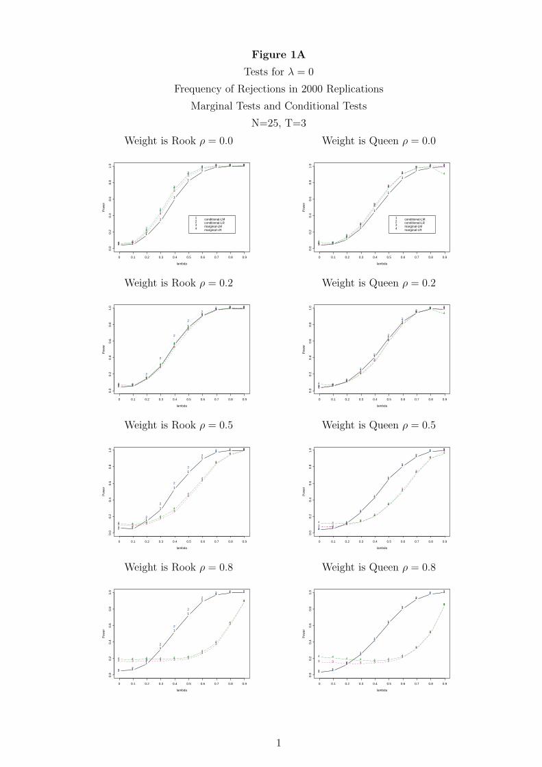
Figure 1A
Tests for λ = 0
Frequency of Rejections in 2000 Replications
Marginal Tests and Conditional Tests
N=25, T=3
Weight is Rook ρ = 0.0
1 1
1
1
1
1
11 1 1
22
2
2
2
2
2 2 2 2
3 3
3
3
3
3
33 3 3
4 4
4
4
4
4
4 4 4 4
lambda
Pow
er
0.0
0.2
0.4
0.6
0.8
1.0
0 0.1 0.2 0.3 0.4 0.5 0.6 0.7 0.8 0.9
1 conditional-LM2 conditional-LR3 marginal-LM4 marginal-LR
Weight is Queen ρ = 0.0
1 1
1
1
1
1
1
11 1
2 2
2
2
2
2
2
22 2
3 3
3
3
3
3
3
33 3
4 4
4
4
4
4
4
4 4
4
lambda
Pow
er
0.0
0.2
0.4
0.6
0.8
1.0
0 0.1 0.2 0.3 0.4 0.5 0.6 0.7 0.8 0.9
1 conditional-LM2 conditional-LR3 marginal-LM4 marginal-LR
Weight is Rook ρ = 0.2
1 1
1
1
1
1
1
1 1 1
2 2
2
2
2
2
22 2 2
3 3
3
3
3
3
3
33 3
4 4
4
4
4
4
4
4 4 4
lambda
Pow
er
0.0
0.2
0.4
0.6
0.8
1.0
0 0.1 0.2 0.3 0.4 0.5 0.6 0.7 0.8 0.9
Weight is Queen ρ = 0.2
11
1
1
1
1
1
11 1
2 2
2
2
2
2
2
22 2
3 33
3
3
3
3
33 3
4 44
4
4
4
4
44
4
lambda
Pow
er
0.0
0.2
0.4
0.6
0.8
1.0
0 0.1 0.2 0.3 0.4 0.5 0.6 0.7 0.8 0.9
Weight is Rook ρ = 0.5
1 1
1
1
1
1
1
1 1 1
2 2
2
2
2
2
2
2 2 2
3 3 3
3
3
3
3
3
3
3
4 4 4
4
4
4
4
4
44
lambda
Pow
er
0.0
0.2
0.4
0.6
0.8
1.0
0 0.1 0.2 0.3 0.4 0.5 0.6 0.7 0.8 0.9
Weight is Queen ρ = 0.5
1 1
1
1
1
1
1
1
1 1
2 22
2
2
2
2
2
2 2
3 3 33
3
3
3
3
3
3
4 4 4 4
4
4
4
4
44
lambda
Pow
er
0.0
0.2
0.4
0.6
0.8
1.0
0 0.1 0.2 0.3 0.4 0.5 0.6 0.7 0.8 0.9
Weight is Rook ρ = 0.8
1 1
1
1
1
1
1
11 1
22
2
2
2
2
2
2 2 2
3 3 3 3 3 3
3
3
3
3
4 4 4 4 4 4
4
4
4
4
lambda
Pow
er
0.0
0.2
0.4
0.6
0.8
1.0
0 0.1 0.2 0.3 0.4 0.5 0.6 0.7 0.8 0.9
Weight is Queen ρ = 0.8
1 1
1
1
1
1
1
1
1 1
2 2
2
2
2
2
2
2
2 2
3 3 3 3 3 33
3
3
3
4 4 4 4 4 44
4
4
4
lambda
Pow
er
0.0
0.2
0.4
0.6
0.8
1.0
0 0.1 0.2 0.3 0.4 0.5 0.6 0.7 0.8 0.9
1
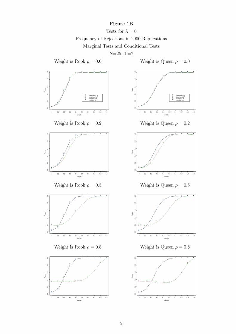
Figure 1B
Tests for λ = 0
Frequency of Rejections in 2000 Replications
Marginal Tests and Conditional Tests
N=25, T=7
Weight is Rook ρ = 0.0
1
1
1
1
11 1 1 1 1
2
2
2
2
2 2 2 2 2 2
3
3
3
3
3 3 3 3 3 3
4
4
4
4
4 4 4 4 4 4
lambda
Pow
er
0.0
0.2
0.4
0.6
0.8
1.0
0 0.1 0.2 0.3 0.4 0.5 0.6 0.7 0.8 0.9
1 conditional-LM2 conditional-LR3 marginal-LM4 marginal-LR
Weight is Queen ρ = 0.0
1
1
1
1
1
1 1 1 1 1
2
2
2
2
2
2 2 2 2 2
3
3
3
3
3
3 3 3 3 3
44
4
4
4
4 4 4 4 4
lambda
Pow
er
0.0
0.2
0.4
0.6
0.8
1.0
0 0.1 0.2 0.3 0.4 0.5 0.6 0.7 0.8 0.9
1 conditional-LM2 conditional-LR3 marginal-LM4 marginal-LR
Weight is Rook ρ = 0.2
1
1
1
1
11 1 1 1 1
2
2
2
2
22 2 2 2 2
3
3
3
3
3
3 3 3 3 3
4
4
4
4
4
4 4 4 4 4
lambda
Pow
er
0.0
0.2
0.4
0.6
0.8
1.0
0 0.1 0.2 0.3 0.4 0.5 0.6 0.7 0.8 0.9
Weight is Queen ρ = 0.2
11
1
1
1
1 1 1 1 1
22
2
2
2
2 2 2 2 2
3 3
3
3
3
33 3 3 3
4 4
4
4
4
4
4 4 4 4
lambda
Pow
er
0.0
0.2
0.4
0.6
0.8
1.0
0 0.1 0.2 0.3 0.4 0.5 0.6 0.7 0.8 0.9
Weight is Rook ρ = 0.5
1
1
1
1
11 1 1 1 1
2
2
2
2
22 2 2 2 2
3 33
3
3
3
3
3 3 3
4 44
4
4
4
4
4 4 4
lambda
Pow
er
0.0
0.2
0.4
0.6
0.8
1.0
0 0.1 0.2 0.3 0.4 0.5 0.6 0.7 0.8 0.9
Weight is Queen ρ = 0.5
1
1
1
1
1
1 1 1 1 1
2
2
2
2
2
2 2 2 2 2
3 33
3
3
3
3
3 3 3
44
4
4
4
4
4
44 4
lambda
Pow
er
0.0
0.2
0.4
0.6
0.8
1.0
0 0.1 0.2 0.3 0.4 0.5 0.6 0.7 0.8 0.9
Weight is Rook ρ = 0.8
1
1
1
1
11 1 1 1 1
2
2
2
2
22 2 2 2 2
3 3 3 33
3
3
3
3
3
4 4 4 44 4
4
4
4
4
lambda
Pow
er
0.0
0.2
0.4
0.6
0.8
1.0
0 0.1 0.2 0.3 0.4 0.5 0.6 0.7 0.8 0.9
Weight is Queen ρ = 0.8
1
1
1
1
1
1 1 1 1 1
2
2
2
2
2
2 2 2 2 2
3 3 33 3 3
3
3
3
3
44 4
4 4 4
4
4
4
4
lambda
Pow
er
0.0
0.2
0.4
0.6
0.8
1.0
0 0.1 0.2 0.3 0.4 0.5 0.6 0.7 0.8 0.9
2
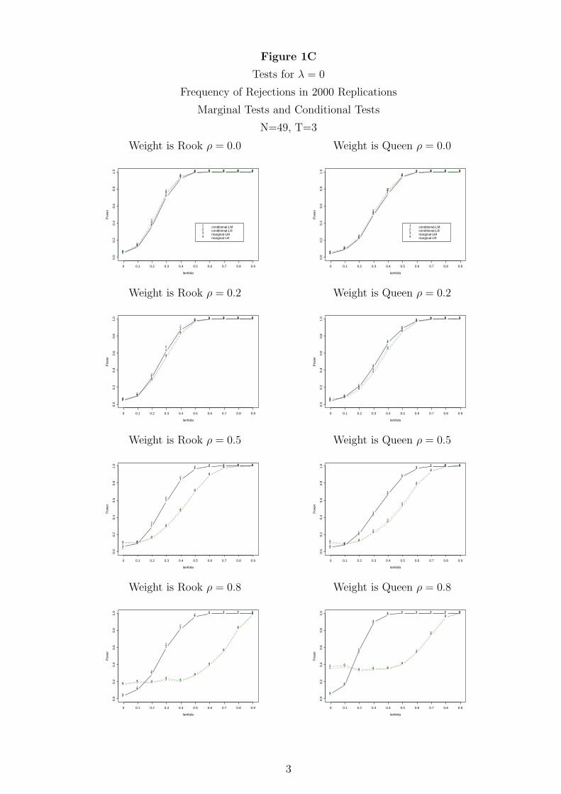
Figure 1C
Tests for λ = 0
Frequency of Rejections in 2000 Replications
Marginal Tests and Conditional Tests
N=49, T=3
Weight is Rook ρ = 0.0
1
1
1
1
1
1 1 1 1 1
2
2
2
2
22 2 2 2 2
3
3
3
3
33 3 3 3 3
4
4
4
4
44 4 4 4 4
lambda
Pow
er
0.0
0.2
0.4
0.6
0.8
1.0
0 0.1 0.2 0.3 0.4 0.5 0.6 0.7 0.8 0.9
1 conditional-LM2 conditional-LR3 marginal-LM4 marginal-LR
Weight is Queen ρ = 0.0
11
1
1
1
11 1 1 1
22
2
2
2
22 2 2 2
3
3
3
3
3
33 3 3 3
44
4
4
4
44 4 4 4
lambda
Pow
er
0.0
0.2
0.4
0.6
0.8
1.0
0 0.1 0.2 0.3 0.4 0.5 0.6 0.7 0.8 0.9
1 conditional-LM2 conditional-LR3 marginal-LM4 marginal-LR
Weight is Rook ρ = 0.2
11
1
1
1
1 1 1 1 1
2
2
2
2
2
2 2 2 2 2
33
3
3
3
33 3 3 3
44
4
4
4
44 4 4 4
lambda
Pow
er
0.0
0.2
0.4
0.6
0.8
1.0
0 0.1 0.2 0.3 0.4 0.5 0.6 0.7 0.8 0.9
Weight is Queen ρ = 0.2
11
1
1
1
1
1 1 1 1
22
2
2
2
2
2 2 2 2
33
3
3
3
3
33 3 3
4 4
4
4
4
4
44 4 4
lambda
Pow
er
0.0
0.2
0.4
0.6
0.8
1.0
0 0.1 0.2 0.3 0.4 0.5 0.6 0.7 0.8 0.9
Weight is Rook ρ = 0.5
11
1
1
1
11 1 1 1
2
2
2
2
2
2 2 2 2 2
3 33
3
3
3
3
3 3 3
4 4
4
4
4
4
4
4 4 4
lambda
Pow
er
0.0
0.2
0.4
0.6
0.8
1.0
0 0.1 0.2 0.3 0.4 0.5 0.6 0.7 0.8 0.9
Weight is Queen ρ = 0.5
11
1
1
1
1
1 1 1 1
22
2
2
2
2
22 2 2
3 33
3
3
3
3
33 3
44
4
4
4
4
4
4
4 4
lambda
Pow
er
0.0
0.2
0.4
0.6
0.8
1.0
0 0.1 0.2 0.3 0.4 0.5 0.6 0.7 0.8 0.9
Weight is Rook ρ = 0.8
1
1
1
1
1
11 1 1 1
2
2
2
2
2
22 2 2 2
33 3
3 3
3
3
3
3
3
44 4
4 4
4
4
4
4
4
lambda
Pow
er
0.0
0.2
0.4
0.6
0.8
1.0
0 0.1 0.2 0.3 0.4 0.5 0.6 0.7 0.8 0.9
Weight is Queen ρ = 0.8
1
1
1
1
1 1 1 1 1 1
2
2
2
2
2 2 2 2 2 2
3 33 3 3
3
3
3
33
4 44 4 4
4
4
4
44
lambda
Pow
er
0.0
0.2
0.4
0.6
0.8
1.0
0 0.1 0.2 0.3 0.4 0.5 0.6 0.7 0.8 0.9
3
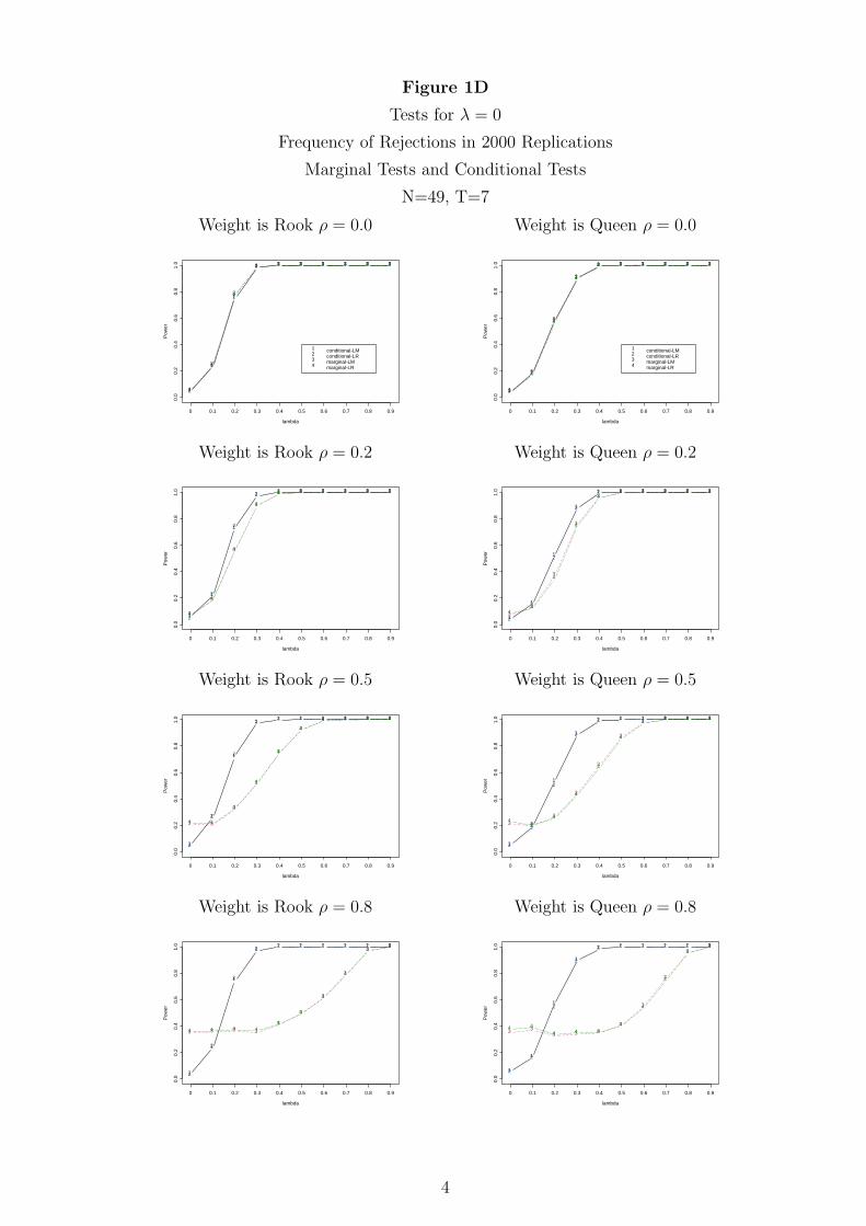
Figure 1D
Tests for λ = 0
Frequency of Rejections in 2000 Replications
Marginal Tests and Conditional Tests
N=49, T=7
Weight is Rook ρ = 0.0
1
1
1
1 1 1 1 1 1 1
2
2
2
2 2 2 2 2 2 2
3
3
3
3 3 3 3 3 3 3
4
4
4
4 4 4 4 4 4 4
lambda
Pow
er
0.0
0.2
0.4
0.6
0.8
1.0
0 0.1 0.2 0.3 0.4 0.5 0.6 0.7 0.8 0.9
1 conditional-LM2 conditional-LR3 marginal-LM4 marginal-LR
Weight is Queen ρ = 0.0
1
1
1
1
1 1 1 1 1 1
2
2
2
2
2 2 2 2 2 2
3
3
3
3
3 3 3 3 3 3
4
4
4
4
4 4 4 4 4 4
lambda
Pow
er
0.0
0.2
0.4
0.6
0.8
1.0
0 0.1 0.2 0.3 0.4 0.5 0.6 0.7 0.8 0.9
1 conditional-LM2 conditional-LR3 marginal-LM4 marginal-LR
Weight is Rook ρ = 0.2
1
1
1
11 1 1 1 1 1
2
2
2
2 2 2 2 2 2 2
3
3
3
3
3 3 3 3 3 3
4
4
4
4
4 4 4 4 4 4
lambda
Pow
er
0.0
0.2
0.4
0.6
0.8
1.0
0 0.1 0.2 0.3 0.4 0.5 0.6 0.7 0.8 0.9
Weight is Queen ρ = 0.2
1
1
1
1
1 1 1 1 1 1
2
2
2
2
2 2 2 2 2 2
3
3
3
3
33 3 3 3 3
44
4
4
44 4 4 4 4
lambda
Pow
er
0.0
0.2
0.4
0.6
0.8
1.0
0 0.1 0.2 0.3 0.4 0.5 0.6 0.7 0.8 0.9
Weight is Rook ρ = 0.5
1
1
1
11 1 1 1 1 1
2
2
2
22 2 2 2 2 2
3 3
3
3
3
3
3 3 3 3
4 4
4
4
4
4
4 4 4 4
lambda
Pow
er
0.0
0.2
0.4
0.6
0.8
1.0
0 0.1 0.2 0.3 0.4 0.5 0.6 0.7 0.8 0.9
Weight is Queen ρ = 0.5
1
1
1
1
1 1 1 1 1 1
2
2
2
2
2 2 2 2 2 2
3 3
3
3
3
3
33 3 3
44
4
4
4
4
44 4 4
lambda
Pow
er
0.0
0.2
0.4
0.6
0.8
1.0
0 0.1 0.2 0.3 0.4 0.5 0.6 0.7 0.8 0.9
Weight is Rook ρ = 0.8
1
1
1
11 1 1 1 1 1
2
2
2
2 2 2 2 2 2 2
3 3 3 3
3
3
3
3
33
4 4 4 44
4
4
4
44
lambda
Pow
er
0.0
0.2
0.4
0.6
0.8
1.0
0 0.1 0.2 0.3 0.4 0.5 0.6 0.7 0.8 0.9
Weight is Queen ρ = 0.8
1
1
1
1
1 1 1 1 1 1
2
2
2
2
2 2 2 2 2 2
3 33 3 3
3
3
3
33
4 44 4 4
4
4
4
44
lambda
Pow
er
0.0
0.2
0.4
0.6
0.8
1.0
0 0.1 0.2 0.3 0.4 0.5 0.6 0.7 0.8 0.9
4

Table 2Tests for ¾2
¹ = 0
Frequency of Rejections in 2000 Replications½ = 0:0
Hb0 ;¾2¹ = 0 (assuming ¸ = 0) He0 ;¾2¹ = 0(assuming ¸ 6= 0)
two-sided one-sided one-sidedN, T W ¸ LMG LRG LM1 SLM1 LR1 LM¤
¹ LR¤¹
25, 3 Rook 0.0 0.037 0.014 0.038 0.038 0.045 0.036 0.0270.1 0.052 0.020 0.044 0.047 0.050 0.043 0.0410.2 0.044 0.015 0.039 0.045 0.045 0.040 0.0390.3 0.055 0.023 0.044 0.049 0.047 0.040 0.0360.4 0.058 0.023 0.046 0.049 0.054 0.031 0.0390.5 0.069 0.017 0.043 0.046 0.048 0.041 0.0380.6 0.100 0.031 0.060 0.067 0.067 0.043 0.0380.7 0.143 0.043 0.067 0.070 0.075 0.043 0.0350.8 0.215 0.050 0.074 0.080 0.083 0.040 0.0340.9 0.341 0.055 0.068 0.074 0.072 0.036 0.035
25, 3 Queen 0.0 0.038 0.016 0.037 0.043 0.042 0.039 0.0330.1 0.045 0.020 0.042 0.046 0.050 0.036 0.0410.2 0.044 0.020 0.044 0.045 0.053 0.045 0.0410.3 0.058 0.020 0.043 0.043 0.051 0.039 0.0400.4 0.054 0.017 0.038 0.041 0.043 0.030 0.0300.5 0.083 0.033 0.054 0.062 0.062 0.038 0.0420.6 0.089 0.032 0.055 0.060 0.058 0.041 0.0340.7 0.154 0.041 0.068 0.073 0.072 0.044 0.0300.8 0.239 0.038 0.057 0.066 0.063 0.042 0.0490.9 0.388 0.033 0.039 0.045 0.051 0.031 0.035
25, 7 Rook 0.0 0.053 0.020 0.052 0.058 0.059 0.043 0.0420.1 0.045 0.018 0.045 0.047 0.053 0.039 0.0300.2 0.033 0.011 0.035 0.039 0.033 0.051 0.0320.3 0.051 0.018 0.049 0.050 0.051 0.045 0.0440.4 0.063 0.022 0.046 0.046 0.047 0.051 0.0360.5 0.062 0.018 0.044 0.044 0.046 0.052 0.0390.6 0.100 0.023 0.051 0.050 0.055 0.066 0.0460.7 0.168 0.035 0.056 0.059 0.058 0.050 0.0360.8 0.257 0.032 0.050 0.050 0.050 0.061 0.0490.9 0.510 0.017 0.024 0.024 0.023 0.050 0.035
25, 7 Queen 0.0 0.059 0.022 0.059 0.057 0.058 0.052 0.0440.1 0.043 0.014 0.038 0.041 0.043 0.039 0.0310.2 0.036 0.014 0.041 0.039 0.039 0.053 0.0370.3 0.050 0.012 0.045 0.044 0.049 0.055 0.0410.4 0.050 0.014 0.040 0.044 0.040 0.061 0.0460.5 0.069 0.025 0.050 0.054 0.049 0.053 0.0390.6 0.089 0.023 0.036 0.036 0.041 0.042 0.0300.7 0.151 0.022 0.040 0.038 0.041 0.049 0.0450.8 0.307 0.015 0.030 0.030 0.030 0.052 0.0510.9 0.589 0.008 0.014 0.014 0.014 0.042 0.057
14
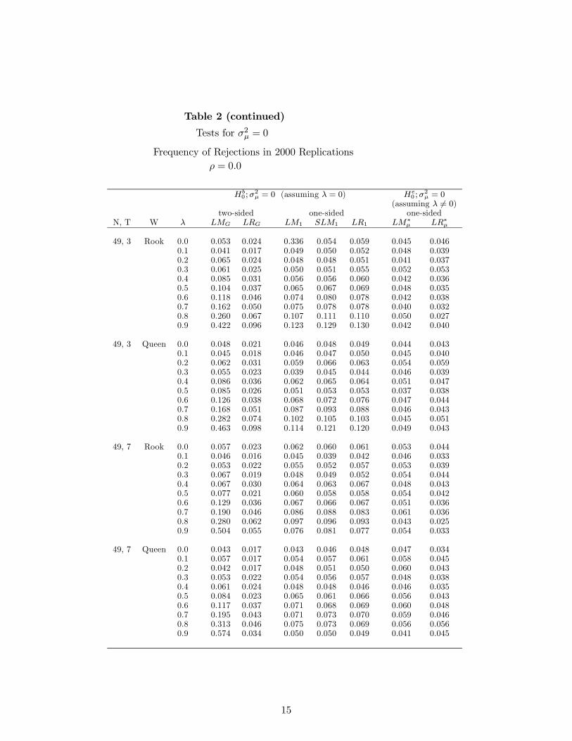
Table 2 (continued)Tests for ¾2
¹ = 0
Frequency of Rejections in 2000 Replications½ = 0:0
Hb0 ;¾2¹ = 0 (assuming ¸ = 0) He0 ;¾2¹ = 0(assuming ¸ 6= 0)
two-sided one-sided one-sidedN, T W ¸ LMG LRG LM1 SLM1 LR1 LM¤
¹ LR¤¹
49, 3 Rook 0.0 0.053 0.024 0.336 0.054 0.059 0.045 0.0460.1 0.041 0.017 0.049 0.050 0.052 0.048 0.0390.2 0.065 0.024 0.048 0.048 0.051 0.041 0.0370.3 0.061 0.025 0.050 0.051 0.055 0.052 0.0530.4 0.085 0.031 0.056 0.056 0.060 0.042 0.0360.5 0.104 0.037 0.065 0.067 0.069 0.048 0.0350.6 0.118 0.046 0.074 0.080 0.078 0.042 0.0380.7 0.162 0.050 0.075 0.078 0.078 0.040 0.0320.8 0.260 0.067 0.107 0.111 0.110 0.050 0.0270.9 0.422 0.096 0.123 0.129 0.130 0.042 0.040
49, 3 Queen 0.0 0.048 0.021 0.046 0.048 0.049 0.044 0.0430.1 0.045 0.018 0.046 0.047 0.050 0.045 0.0400.2 0.062 0.031 0.059 0.066 0.063 0.054 0.0590.3 0.055 0.023 0.039 0.045 0.044 0.046 0.0390.4 0.086 0.036 0.062 0.065 0.064 0.051 0.0470.5 0.085 0.026 0.051 0.053 0.053 0.037 0.0380.6 0.126 0.038 0.068 0.072 0.076 0.047 0.0440.7 0.168 0.051 0.087 0.093 0.088 0.046 0.0430.8 0.282 0.074 0.102 0.105 0.103 0.045 0.0510.9 0.463 0.098 0.114 0.121 0.120 0.049 0.043
49, 7 Rook 0.0 0.057 0.023 0.062 0.060 0.061 0.053 0.0440.1 0.046 0.016 0.045 0.039 0.042 0.046 0.0330.2 0.053 0.022 0.055 0.052 0.057 0.053 0.0390.3 0.067 0.019 0.048 0.049 0.052 0.054 0.0440.4 0.067 0.030 0.064 0.063 0.067 0.048 0.0430.5 0.077 0.021 0.060 0.058 0.058 0.054 0.0420.6 0.129 0.036 0.067 0.066 0.067 0.051 0.0360.7 0.190 0.046 0.086 0.088 0.083 0.061 0.0360.8 0.280 0.062 0.097 0.096 0.093 0.043 0.0250.9 0.504 0.055 0.076 0.081 0.077 0.054 0.033
49, 7 Queen 0.0 0.043 0.017 0.043 0.046 0.048 0.047 0.0340.1 0.057 0.017 0.054 0.057 0.061 0.058 0.0450.2 0.042 0.017 0.048 0.051 0.050 0.060 0.0430.3 0.053 0.022 0.054 0.056 0.057 0.048 0.0380.4 0.061 0.024 0.048 0.048 0.046 0.046 0.0350.5 0.084 0.023 0.065 0.061 0.066 0.056 0.0430.6 0.117 0.037 0.071 0.068 0.069 0.060 0.0480.7 0.195 0.043 0.071 0.073 0.070 0.059 0.0460.8 0.313 0.046 0.075 0.073 0.069 0.056 0.0560.9 0.574 0.034 0.050 0.050 0.049 0.041 0.045
15
4 CONCLUSION
It is clear from the extensive Monte Carlo experiments performed that the spatial economet-
rics literature should not ignore the heterogeneity across cross-sectional units when testing
for the presence of spatial error correlation. Similarly, the panel data econometrics literature
should not ignore the spatial error correlation when testing for the presence of random re-
gional e¤ects. Both joint and conditional LM tests have been derived in this paper that are
easy to implement and that perform better in terms of size and power than the one-directional
LM tests. The latter tests ignore the random regional e¤ects when testing for spatial error
correlation or ignore spatial error correlation when testing for random regional e¤ects. This
paper does not consider testing for spatial lag dependence and random regional e¤ects in a
panel. This should be the subject of future research. Also, the results in the paper should
be tempered by the fact that the N = 25; 49 used in our Monte Carlo experiments may be
small for a typical micro panel. Larger N will probably improve the performance of these
tests whose critical values are based on their large sample distributions. However, it will
also increase the computation di¢culty and accuracy of the eigenvalues of the big weighting
matrix W . Finally, it is important to point out that the asymptotic distribution of our test
statistics were not explicitly derived in the paper but that they are likely to hold under a
similar set of low level assumptions developed by Kelejian and Prucha (2001).
5 REFERENCES
Anselin, L. (1988). Spatial Econometrics: Methods and Models (Kluwer Academic Publish-
ers, Dordrecht).
Anselin, L. (1999). Rao’s score tests in spatial econometrics. Journal of Statistical Planning
and Inference, (forthcoming).
Anselin, L. and A.K. Bera (1998). Spatial dependence in linear regression models with an
introduction to spatial econometrics. In A. Ullah and D.E.A. Giles, (eds.), Handbook
of Applied Economic Statistics, Marcel Dekker, New York.
Anselin, L. , A.K. Bera, R. Florax and M.J. Yoon (1996). Simple diagnostic tests for spatial
dependence. Regional Science and Urban Economics 26, 77-104.
Anselin, L and S. Rey (1991). Properties of tests for spatial dependence in linear regression
models. Geographical Analysis 23, 112-131.
16
Anselin, L. and R. Florax (1995). Small sample properties of tests for spatial dependence
in regression models: Some further results. In L. Anselin and R. Florax, (eds.), New
Directions in Spatial Econometrics, Springer-Verlag, Berlin, pp. 21-74.
Baltagi, B.H. (2001). Econometrics Analysis of Panel Data (Wiley, Chichester).
Baltagi, B.H., Y.J. Chang, and Q. Li (1992). Monte Carlo results on several new and
existing tests for the error component model. Journal of Econometrics 54, 95-120.
Baltagi, B.H. and D. Li (1999). Prediction in the panel data model with spatial correla-
tion. In L. Anselin and R.J.G.M. Florax (eds.), New Advances in Spatial Econometrics,
(forthcoming).
Bell, K.P. and N.R. Bockstael (2000). Applying the generalized-moments estimation ap-
proach to spatial problems involving microlevel data. Review of Economics and Statis-
tics 82, 72-82.
Breusch, T.S. and A.R. Pagan (1980). The Lagrange Multiplier test and its application to
model speci…cation in econometrics. Review of Economic Studies 47, 239-254.
Case, A.C. (1991). Spatial patterns in household demand. Econometrica 59, 953-965.
Case, A.C., J. Hines, Jr. and H. Rosen (1993). Budget spillovers and …scal policy indepen-
dence: Evidence from the states. Journal of Public Economics 52, 285-307.
Conley, T.G. (1999). GMM estimation with cross sectional dependence. Journal of Econo-
metrics 92, 1-45.
De Long, J.B. and L.H. Summers (1991). Equipment investment and economic growth.
Quarterly Journal of Economics 106, 445-502.
Driscoll, J. and A. Kraay (1998). Consistent covariance matrix estimation with spatially
dependent panel data. Review of Economics and Statistics 80, 549-560.
Evans, M.A. and M.L. King (1985). Critical value approximations for tests of linear regres-
sion disturbances. Review of Economic Studies 47, 329-254.
Gourieroux, C., A. Holly and A. Monfort (1982). Likelihood ratio test, Wald test, and Kuhn-
Tucker test in linear models with inequality constraints on the regression parameters.
Econometrica 50, 63-80.
Hartley, H.O. and J.N.K. Rao (1967). Maximum likelihood estimation for the mixed analysis
of variance model. Biometrika 54, 93-108.
17
Harville, D.A. (1977). Maximum likelihood approaches to variance component estimation
and to related problems. Journal of the American Statistical Association 72, 320-338.
Hemmerle, W.J. and H.O. Hartley (1973). Computing maximum likelihood estimates for
the mixed A.O.V. model using the W-transformation. Technometrics 15, 819-831.
Holtz-Eakin, D. (1994). Public-sector capital and the productivity puzzle. Review of Eco-
nomics and Statistics 76, 12-21.
Honda, Y. (1985). Testing the error components model with non-normal disturbances.
Review of Economic Studies 52, 681-690.
Islam, N. (1995). Growth empirics: A panel data approach. Quarterly Journal of Economics
110, 1127-1170.
Kelejian, H.H. and I.R. Prucha (1999). A generalized moments estimator for the autore-
gressive parameter in a spatial model. International Economic Review 40, 509-533.
Kelejian, H.H. and I.R. Prucha (2001). On the asymptotic distribution of the Moran I test
with applications. Journal of Econometrics 104, 219-257.
Kelejian H.H and D.P. Robinson (1992). Spatial autocorrelation: A new computationally
simple test with an application to per capita county police expenditures. Regional
Science and Urban Economics 22, 317-331.
Moulton, B.R. and W.C. Randolph (1989). Alternative tests of the error components model.
Econometrica 57, 685-693.
Nerlove, M. (1971). Further evidence on the estimation of dynamic economic relations from
a time-series of cross-sections. Econometrica 39, 359-382.
Pinkse, J. (1998). Asymptotic properties of Moran and related tests and a test for spatial
correlation in probit models, working paper, Department of Economics, University of
British Columbia.
Pinkse, J. (1999). Moran-‡avoured tests with nuisance parameters: Examples. In L. Anselin
and R.J.G.M. Florax (eds.), New Advances in Spatial Econometrics, (forthcoming).
Wansbeek, T.J. and A. Kapteyn (1983). A note on spectral decomposition and maximum
likelihood estimation of ANOVA models with balanced data. Statistics and Probability
Letters 1, 213-215.
18
Appendix A.1: Joint LM testThis appendix derives the joint LM test for spatial error correlation and random regional
e¤ects. The null hypothesis is given by Ha0 : ¾2¹ = ¸ = 0. Let µ = (¾2
º ; ¾2¹; ¸)0: Note that
the part of the information matrix corresponding to ¯ will be ignored in computing the LM
statistic, since the information matrix between the µ and ¯ parameters will be block diagonal
and the …rst derivatives with respect to ¯ evaluated at the restricted MLE will be zero. The
LM statistic is given by
LM = ~D0µ~J¡1µ ~Dµ; (A.1)
where ~Dµ = (@L=@µ)(~µ) is a 3 £ 1 vector of partial derivatives with respect to each element
of µ, evaluated at the restricted MLE ~µ: Also, ~J = E[¡@2L=@µ@µ0](~µ) is the information
matrix corresponding to µ, evaluated at the restricted MLE ~µ. Under the null hypothesis, the
variance-covariance matrix reduces to ¾2ºITN and the restricted MLE of ¯ is ~
OLS , so that
~u = y ¡ X 0 ~OLS are the OLS residuals and ~¾2
º = ~u0~u=NT .
Hartley and Rao(1967) or Hemmerle and Hartley(1973) give a useful general formula to obtain~Dµ:
@L=@µr = ¡12tr[¡1u (@u=@µr)] +
12[u0¡1u (@u=@µr)¡1u u]; (A.2)
for r = 1; 2; 3. It is easy to check that @u=@¾2º = IT (B0B)¡1, @u=@¾2
¹ = JT INand @u=@¸ = ¾2
º [IT (B0B)¡1(W 0B + B0W )(B0B)¡1] using the fact that @(B0B)¡1=@¸ =
(B0B)¡1(W 0B + B0W )(B0B)¡1, see Anselin (1988, p.164).
Under Ha0 , we get
¡1u jHa0 =1¾2ºIT IN ; (A.3)
@u@¾2ºjHa0 = IT IN ;
@u@¾2¹jHa0 = JT IN ;
@u@¸
jHa0 = ¾2ºIT (W 0 + W ):
This uses the fact that B = IN under Ha0 . Using (A.2), we obtain
19
@L@¾2ºjHa0 = ¡1
2tr[
1~¾2º(IT (B0B)¡1)] +
12[~u0
1~¾4º(IT (B0B)¡1)~u];
= ¡12tr[
1~¾2ºINT ] +
12[~u0~u~¾4º
] = 0;
@L@¾2¹jHa0 = D(~¾2
¹) =NT2~¾2º
¡ ~u0(JT IN )~u~u0~u
¡ 1¢;
@L@¸
jHa0 = D(~) =NT2
~u0(IT (W + W 0))~u~u0~u
= NT~u0(IT W )~u
~u0~u:
Therefore, the score with respect to µ, evaluated at the restricted MLE is given by
~Dµ =
266664
0
D(~¾2¹)
D(~)
377775
=
266664
0
NT2~¾2º
( ~u0(JTIN )~u
~u0~u ¡ 1)
NT ~u0(ITW )~u~u0~u
377775
: (A.4)
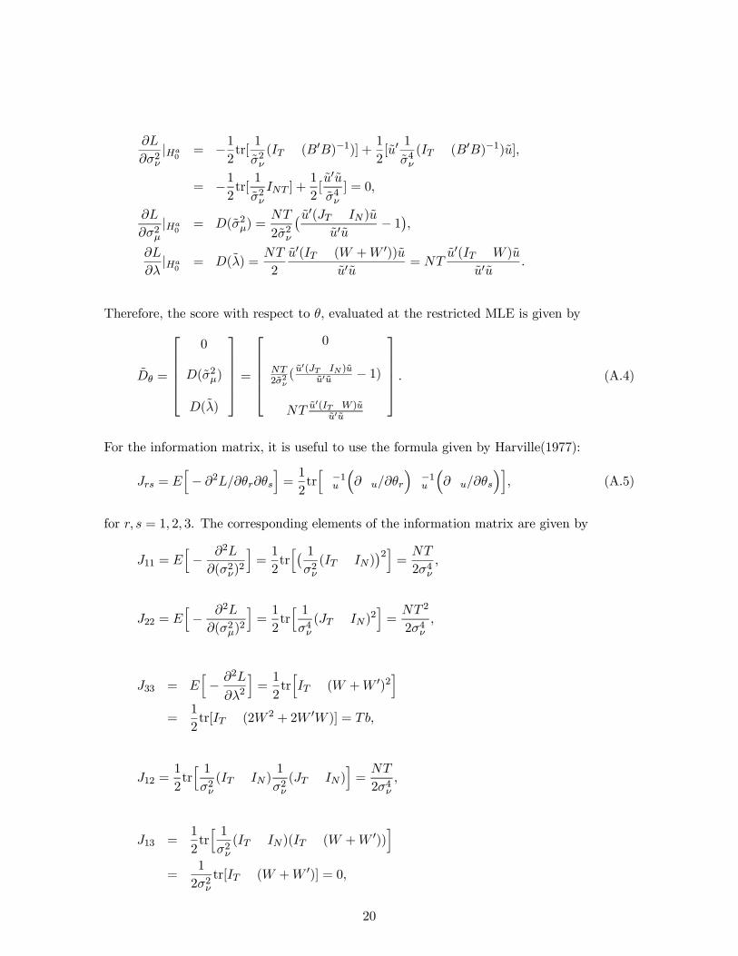
For the information matrix, it is useful to use the formula given by Harville(1977):
Jrs = Eh
¡ @2L=@µr@µsi
=12tr
h¡1u
³@u=@µr
´¡1u
³@u=@µs
´i; (A.5)
for r; s = 1; 2; 3. The corresponding elements of the information matrix are given by
J11 = Eh
¡ @2L@(¾2
º)2i
=12tr
h¡ 1¾2º(IT IN)
¢2i =NT2¾4º;
J22 = Eh
¡ @2L@(¾2
¹)2i
=12tr
h 1¾4º(JT IN)2
i=
NT 2
2¾4º
;
J33 = Eh
¡ @2L@¸2
i=
12tr
hIT (W + W 0)2
i
=12tr[IT (2W 2 + 2W 0W )] = Tb;
J12 =12tr
h 1¾2º(IT IN)
1¾2º(JT IN)
i=
NT2¾4º;
J13 =12tr
h 1¾2º(IT IN)(IT (W + W 0))
i
=1
2¾2ºtr[IT (W + W 0)] = 0;
20
J23 =12tr
h 1¾2º(JT IN)(IT (W + W 0))
i
=1
2¾2ºtr[JT (W + W 0)] = 0;
where the result that J13 = J23 = 0 follows from the fact that the diagonal elements of W
are 0 and J33 uses the fact that tr(W 2) = tr(W 02) and b = tr(W 2 + W 0W ).
Therefore, the information matrix evaluated under Ha0 is given by
~Jµ =NT2~¾4º
266664
1 1 0
1 T 0
0 0 2b~¾4ºN
377775
; (A.6)
using (A.1), we get
LMJ =·0;
NT2~¾2ºG;NTH
¸(2~¾4º
NT)
264
TT¡1 ¡ 1
T¡1 0¡ 1T¡1
1T¡1 0
0 0 N2b~¾4º
375
24
0NT2~¾2º
GNTH
35
=NT
2(T ¡ 1)G2 +
N2Tb
H2: (A.7)
where G = ~u0(JTIN )~u~u0~u ¡ 1 and H = ~u0(ITW )~u
~u0~u as descibed in (2.11).
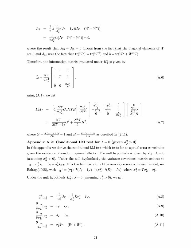
Appendix A.2: Conditional LM test for ¸ = 0 (given ¾2¹ > 0)In this appendix we derive the conditional LM test which tests for no spatial error correlation
given the existence of random regional e¤ects. The null hypothesis is given by Hd0 : ¸ = 0
(assuming ¾2¹ > 0). Under the null hyphothesis, the variance-covariance matrix reduces to
0 = ¾2¹JT IN + ¾2
ºINT . It is the familiar form of the one-way error component model, see
Baltagi(1995), with ¡10 = (¾21)¡1( ¹JT IN ) + (¾2
º)¡1(ET IN), where ¾21 = T¾2
¹ + ¾2º .
Under the null hypothesis Hd0 : ¸ = 0 (assuming ¾2¹ > 0), we get
¡1u jHd0 =¡ 1¾21
¹JT +1¾2ºET
¢ IN ; (A.8)
@u@¾2ºjHd0 = IT IN ; (A.9)
@u@¾2¹jHd0 = JT IN ; (A.10)
@u@¸
jHd0 = ¾2ºIT (W + W 0): (A.11)
21
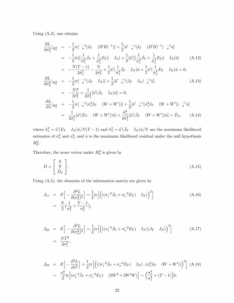
Using (A.2), one obtains
@L@¾2ºjHd0 = ¡1
2tr[¡1u (IT (B0B)¡1)] +
12[u0¡1u (IT (B0B)¡1)¡1u u]
= ¡12tr[
¡ 1¾21
¹JT +1¾2ºET
¢ IN ] +
12[u0[
¡ 1¾41
¹JT +1¾4ºET
¢ IN ]u] (A.12)
= ¡N(T ¡ 1)2¾2º
¡ N2¾2
1+
12u0(
1¾41
¹JT IN)u +12u0(
1¾4ºET IN)u = 0;
@L@¾2¹jHd0 = ¡1
2tr[¡1u (JT IN)] +
12[u0¡1u (JT IN)¡1u u] (A.13)
= ¡NT2¾2
1+
12¾4
1[u0( ¹JT IN)u] = 0;
@L@¸
jHd0 = ¡12tr[¡1u (¾2
ºIT (W + W 0))] +12[u0¡1u (¾2
ºIT (W + W 0))¡1u u]
=1
2¾2º[u0(ET (W + W 0))u] +
¾2º
2¾41[u0( ¹JT (W + W 0))u] = D¸; (A.14)
where ¾2º = u0(ET IN)u=N(T ¡ 1) and ¾2
1 = u0( ¹JT IN)u=N are the maximum likelihood
estimates of ¾2º and ¾2
1, and u is the maximum likelihood residual under the null hypothesis
Hd0 .
Therefore, the score vector under Hd0 is given by
D =
24
00
D¸
35 : (A.15)
Using (A.5), the elements of the information matrix are given by
J11 = Eh
¡ @2L@(¾2
º)2i
=12tr
h³((¾¡21
¹JT + ¾¡2º ET ) IN)´2i
(A.16)
=N2
¡ 1¾41
+T ¡ 1
¾4º
¢;
J22 = Eh
¡ @2L@(¾2
¹)2i
=12tr
h³((¾¡21
¹JT + ¾¡2º ET ) IN )(JT IN)´2i
(A.17)
=NT 2
2¾41
;
J33 = Eh
¡ @2L@¸2
i=
12tr
h³((¾¡21
¹JT + ¾¡2º ET ) IN) ¢ (¾2ºIT (W + W 0))
´2i(A.18)
=¾4º2
trh(¾¡41
¹JT + ¾¡4º ET ) (2W 2 + 2W 0W )i
=³¾4º
¾41
+ (T ¡ 1)´b;
22
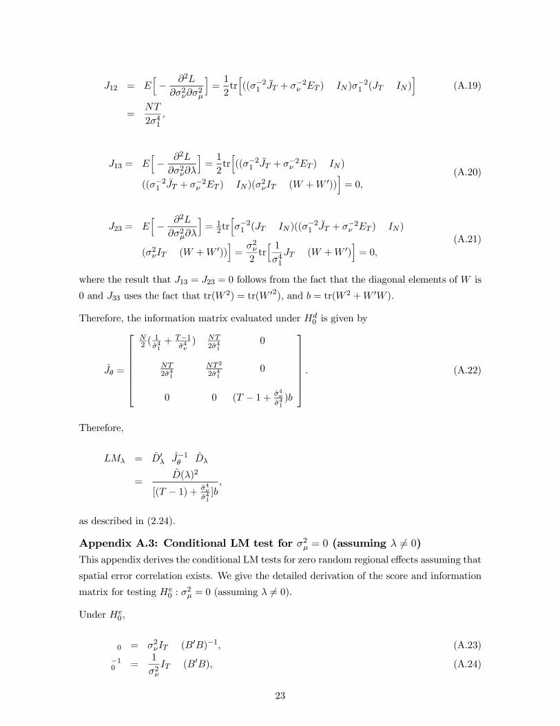
J12 = Eh
¡ @2L@¾2º@¾2
¹
i=
12tr
h((¾¡21
¹JT + ¾¡2º ET ) IN)¾¡21 (JT IN)i
(A.19)
=NT2¾4
1;
J13 = Eh
¡ @2L@¾2º@¸
i=
12tr
h((¾¡21
¹JT + ¾¡2º ET ) IN)
((¾¡21¹JT + ¾¡2º ET ) IN)(¾2
ºIT (W + W 0))i
= 0;(A.20)
J23 = Eh
¡ @2L@¾2¹@¸
i= 1
2trh¾¡21 (JT IN )((¾¡21
¹JT + ¾¡2º ET ) IN)
(¾2ºIT (W + W 0))
i=
¾2º2
trh 1¾41JT (W + W 0)
i= 0;
(A.21)
where the result that J13 = J23 = 0 follows from the fact that the diagonal elements of W is
0 and J33 uses the fact that tr(W 2) = tr(W 02), and b = tr(W 2 + W 0W ).
Therefore, the information matrix evaluated under Hd0 is given by
Jµ =
26666664
N2 ( 1¾41
+ T¡1¾4º
) NT2¾41
0
NT2¾41
NT 22¾41
0
0 0 (T ¡ 1 + ¾4º¾41
)b
37777775
: (A.22)
Therefore,
LM¸ = D0¸ J¡1µ D¸
=D(¸)2
[(T ¡ 1) + ¾4º¾41
]b;
as described in (2.24).
Appendix A.3: Conditional LM test for ¾2¹ = 0 (assuming ¸ 6= 0)This appendix derives the conditional LM tests for zero random regional e¤ects assuming that
spatial error correlation exists. We give the detailed derivation of the score and information
matrix for testing He0 : ¾2¹ = 0 (assuming ¸ 6= 0).
Under He0 ,
0 = ¾2ºIT (B0B)¡1; (A.23)
¡10 =1¾2ºIT (B0B); (A.24)
23

and
@u@¾2¹
¯¯He0
= JT IN ; (A.25)
@u@¾2º
¯¯He0
= IT ( bB0 bB)¡1; (A.26)
@u@¸
¯¯He0
= b¾2ºIT ( bB0 bB)¡1(W 0 bB + bB0W )( bB0 bB)¡1; (A.27)
where bB = IN ¡ bW and b is the MLE of ¸ under He0 . Using (A.2), we get
D¹ =@L@¾2¹
¯¯He0
= ¡ T2b¾2ºtr( bB0 bB) +
12b¾4ºbu0[JT ( bB0 bB)2]bu: (A.28)
This uses the fact that
¡1u@u@¾2¹
¯¯He0
=¡ 1¾2ºIT bB0 bB
¢¡JT IN
¢=
1b¾2ºJT bB0 bB;
¡1u@u@¾2¹¡1u
¯¯He0
=¡ 1b¾2ºJT bB0 bB
¢¡ 1b¾2ºIT bB0 bB
¢=
1b¾4ºJT ( bB0 bB)2;
tr[¡1u@u@¾2¹]¯¯He0
=1b¾2ºtr[JT bB0 bB] =
Tb¾2ºtr[ bB0 bB]:
Similarly
@L@¾2º
¯¯He0
= ¡TN2b¾2º
+1
2b¾4ºbu0[IT ( bB0 bB)]bu = 0; (A.29)
which yields
¾2º =
u0[IT bB0 bB]uTN
:
This uses the fact that
¡1u@u@¾2º
¯¯He0
=¡ 1b¾2ºIT bB0 bB
¢¡IT ( bB0 bB)¡1
¢=
1b¾2ºIT IN ;
¡1u@u@¾2º¡1u
¯¯He0
=¡ 1b¾2ºIT IN
¢¡ 1b¾2ºIT bB0 bB
¢=
1b¾4ºIT bB0 bB;
tr[¡1u@u@¾2º]¯¯He0
=TNb¾2º
:
Also,
24
@L@¸
¯¯He0
= ¡T2
tr[(W 0 bB + bB0W )( bB0 bB)¡1]
+1
2b¾2ºu[IT (W 0 bB + bB0W )]u = 0;
because
¡1u@u@¸
¯¯He0
=¡ 1
b¾2ºIT bB0 bB
¢¡b¾2ºIT ( bB0 bB)¡1(W 0 bB + bB0W )( bB0 bB)¡1
¢
= IT (W 0 bB + bB0W )( bB0 bB)¡1
¡1u@u@¸
¡1u¯¯He0
= 1b¾2º
IT (W 0 bB + bB0W ):
Therefore, the score vector under He0 is given by
D =
24
00
D¹
35 : (A.30)
The elements of the information matrix for this model using (A.5) are given by
J11 = Eh
¡ @2L@(¾2
º)2i¯¯He0
=12tr
h¡(b¾2º)¡1IT IN
¢2¤ =TN2b¾4º;
J22 = Eh
¡ @2L@¸2
i¯¯He0
=12tr
h¡IT (W 0 bB + bB0W )( bB0 bB)¡1
¢2i
=T2
trh¡
(W 0 bB + bB0W )( bB0 bB)¡1¢2i;
J33 = Eh
¡ @2L@¾2¹
i¯¯He0
=12tr
h¡(b¾2º)¡1JT bB0 bB
¢2i =T 2
2b¾4ºtr[( bB0 bB)2];
J12 = Eh
¡ @2L@¾2º@¸
i¯¯He0
=12tr
h(b¾2º)¡1(IT IN)(IT (W 0 bB + bB0W )( bB0 bB)¡1)
i
=12tr
h(b¾2º)¡1IT (W 0 bB + bB0W )( bB0 bB)¡1)
i
=T
2b¾2ºtr
h(W 0 bB + bB0W )( bB0 bB)¡1
i;
J13 = Eh
¡ @2L@¾2º@¾2
¹
i¯¯He0
=12tr
h(b¾2º)¡1(IT IN)((b¾2
º)¡1JT bB0 bB)
i
=1
2b¾4ºtr[JT bB0 bB] =
T2b¾4ºtr[ bB0 bB];
25

J23 = Eh
¡ @2L@¾2¹@¸
i¯¯He0
=12tr
h(IT (W 0 bB + bB0W )( bB0 bB)¡1)((b¾2
º)¡1JT bB0 bB)
i
=1
2b¾2ºtr[JT (W 0 bB + bB0W )] =
T2b¾2ºtr[W 0 bB + bB0W ];
Jµ =
2664
TN2¾4º
T2¾2º
tr[(W 0 bB + bB0W )( bB0 bB)¡1] T2¾4º
tr[ bB0 bB]T2 tr
£¡(W 0 bB + bB0W )( bB0 bB)¡1
¢2¤ T2¾2º
tr[W 0 bB + bB0W ]T 22¾4º
tr[( bB0 bB)2]
3775 : (A.31)
26