DIPARTIMENTO DI FISICA “ENRICO FERMI”

Corso di Laurea Magistrale in Fisica

Tesi di Laurea

Performance Improvement of the Inertial Sensorsof Advanced Virgo Seismic Isolators

with Digital Techniques

Candidato:

Giovanni CerretaniRelatori:

Dott. Diego PassuelloIng. Alberto Gennai

Anno Accademico 2012/2013

Contents

Abstract 1

Introduction 3

I. Gravitational Waves 7

1. A Little of Theory 91.1. An Introduction to General Relativity . . . . . . . . . . . . . . . . . 9

1.1.1. The Principle of Equivalence . . . . . . . . . . . . . . . . . . . 91.1.2. General Relativity and Einstein’s Field Equations . . . . . . . 10

1.2. Gravitational radiation . . . . . . . . . . . . . . . . . . . . . . . . . . 111.3. The Effects of Gravitational Waves . . . . . . . . . . . . . . . . . . . 13

2. The Search for Gravitational Waves 172.1. The First Indirect Observation: PSR B1913+16 . . . . . . . . . . . . 172.2. BICEP2 and Inflationary Gravitational Radiation . . . . . . . . . . . 192.3. Sources of Gravitational Waves . . . . . . . . . . . . . . . . . . . . . 19

2.3.1. Burst Sources . . . . . . . . . . . . . . . . . . . . . . . . . . . 202.3.2. Periodic Sources . . . . . . . . . . . . . . . . . . . . . . . . . . 222.3.3. Stochastic Background . . . . . . . . . . . . . . . . . . . . . . 242.3.4. The Impracticality of Artificial Sources . . . . . . . . . . . . . 24

2.4. Detectors of Gravitational Waves . . . . . . . . . . . . . . . . . . . . 262.4.1. Weber Bars . . . . . . . . . . . . . . . . . . . . . . . . . . . . 262.4.2. Interferometers . . . . . . . . . . . . . . . . . . . . . . . . . . 26

i

Contents Contents

II. Accelerometer Control 29

3. An Introduction to Control Theory 313.1. Linear Time-Invariant Systems . . . . . . . . . . . . . . . . . . . . . 313.2. Transfer Functions . . . . . . . . . . . . . . . . . . . . . . . . . . . . 323.3. Feedback Control Systems . . . . . . . . . . . . . . . . . . . . . . . . 34

3.3.1. Actual Feedback Controls . . . . . . . . . . . . . . . . . . . . 353.3.2. Advantages and Disadvantages . . . . . . . . . . . . . . . . . 36

3.4. Stability of a Linear System . . . . . . . . . . . . . . . . . . . . . . . 363.4.1. Nyquist Stability Criterion . . . . . . . . . . . . . . . . . . . . 36

4. Digital Filters 374.1. Definitions . . . . . . . . . . . . . . . . . . . . . . . . . . . . . . . . . 374.2. Linear Shift-Invariant Systems . . . . . . . . . . . . . . . . . . . . . . 384.3. Design of Digital Filters from Analog Filters . . . . . . . . . . . . . . 38

5. Seismic Isolation System in Advanced Virgo 415.1. Seismic Noise . . . . . . . . . . . . . . . . . . . . . . . . . . . . . . . 415.2. Superattenuators . . . . . . . . . . . . . . . . . . . . . . . . . . . . . 42

5.2.1. Passive Attenuation . . . . . . . . . . . . . . . . . . . . . . . . 445.2.2. Superattenuator Control System . . . . . . . . . . . . . . . . . 45

5.3. Control System towards Advanced Virgo . . . . . . . . . . . . . . . . 475.3.1. Gyroscope and Tilt Control . . . . . . . . . . . . . . . . . . . 475.3.2. Electronics . . . . . . . . . . . . . . . . . . . . . . . . . . . . . 485.3.3. Control Techniques . . . . . . . . . . . . . . . . . . . . . . . . 50

6. Accelerometer Design and Control 556.1. A Simple Dynamics Description . . . . . . . . . . . . . . . . . . . . . 566.2. Feedback Control . . . . . . . . . . . . . . . . . . . . . . . . . . . . . 586.3. Virgo/Virgo+ Design . . . . . . . . . . . . . . . . . . . . . . . . . . . 606.4. Advanced Virgo Design . . . . . . . . . . . . . . . . . . . . . . . . . . 61

6.4.1. Critical Damping . . . . . . . . . . . . . . . . . . . . . . . . . 63

III. Implementation of the Digital Control 69

7. Measurement of Transfer Functions 717.1. Calibration . . . . . . . . . . . . . . . . . . . . . . . . . . . . . . . . 717.2. Open Loop Transfer Function . . . . . . . . . . . . . . . . . . . . . . 73

7.2.1. LVDT Non-Linearity Effects . . . . . . . . . . . . . . . . . . . 757.3. Closed Loop Transfer Function . . . . . . . . . . . . . . . . . . . . . 76

8. Digital Synthesizer and Demodulation 778.1. Linear Variable Differential Transformers . . . . . . . . . . . . . . . . 77

8.1.1. Operation of a Transformer . . . . . . . . . . . . . . . . . . . 78

ii

Contents

8.2. Demodulation of the LVDT Signal . . . . . . . . . . . . . . . . . . . 808.2.1. Effects of a Quadrature Term . . . . . . . . . . . . . . . . . . 81

8.3. An Algorithm to Demodulate with Phase Locking . . . . . . . . . . . 838.3.1. Stability of the System, Simulations and Limits . . . . . . . . 93

9. Accelerometer Noise Budget 959.1. Process Noise . . . . . . . . . . . . . . . . . . . . . . . . . . . . . . . 959.2. Sensing Noise . . . . . . . . . . . . . . . . . . . . . . . . . . . . . . . 96

9.2.1. Noise on Primary Coil . . . . . . . . . . . . . . . . . . . . . . 969.2.2. Noise on Secondary Coils . . . . . . . . . . . . . . . . . . . . . 97

9.3. Acting Noise . . . . . . . . . . . . . . . . . . . . . . . . . . . . . . . . 999.4. Total Noise Budget . . . . . . . . . . . . . . . . . . . . . . . . . . . . 103

9.4.1. Comparison with Virgo/Virgo+ Analog Control . . . . . . . . 104

10.Conclusions 109

A. Mathematical Tools 111A.1. Laplace Transform . . . . . . . . . . . . . . . . . . . . . . . . . . . . 111

A.1.1. Inverse Laplace Transform . . . . . . . . . . . . . . . . . . . . 111A.1.2. Used Properties . . . . . . . . . . . . . . . . . . . . . . . . . . 111

A.2. Z-Transform . . . . . . . . . . . . . . . . . . . . . . . . . . . . . . . . 112A.2.1. Region of Convergence . . . . . . . . . . . . . . . . . . . . . . 113A.2.2. Inverse Z-transform . . . . . . . . . . . . . . . . . . . . . . . . 113A.2.3. Convolution of Sequences . . . . . . . . . . . . . . . . . . . . 113A.2.4. Used Properties . . . . . . . . . . . . . . . . . . . . . . . . . . 113

A.3. Bilinear Transformation . . . . . . . . . . . . . . . . . . . . . . . . . 114

B. Technical Tools 117B.1. Mechanical Impedances . . . . . . . . . . . . . . . . . . . . . . . . . . 117B.2. Thermal Noise . . . . . . . . . . . . . . . . . . . . . . . . . . . . . . . 118

C. Notes on Seismic Noise 119C.1. An Analytic Approach . . . . . . . . . . . . . . . . . . . . . . . . . . 119

Bibliography 121

Nomenclature 125

iii

Abstract

Gravitational waves, predicted on the basis of the General Relativity, are ripples inthe curvature of space-time that propagate as a wave. The passage of a gravitationalwave induces tiny oscillations in the relative separation between two test masses, thatcan be measured. Nevertheless these oscillations are extremely small, so that only avery sensitive detector is able to measure them. The Advanced Virgo project is amajor upgrade of the 3 km-long interferometric gravitational wave detector Virgo,with the goal of increasing its sensitivity by about one order of magnitude in thewhole detection band. We expect to have a maximum strain amplitude sensitivity of4× 10−24 1√

Hz at ∼ 300Hz. In other words this means that it will be able to detect arelative displacement between mirrors of about 10−20 m, by averaging for one second.This sensitivity should allow to detect several tens of events per year.Among the various ongoing updates, an important improvement is representedby the new electronics used to control the Superattenuators, complex mechanicalstructures that isolate optical elements from seismic noise by a factor 1015 at 1Hz.Using the information of several inertial sensors, a digital control system keeps thestructures as stable as possible. A new board for the Superattenuator control hasbeen designed, that incorporates analog-to-digital and digital-to-analog converters, aField Programmable Gate Array (FPGA) and a Digital Signal Processor (DSP) intoa single unit. This board is enough to handle every single part of the Superattenuatorinertial control. It performs the computation of feedback forces, and is used tosynthesize sine wave to drive the coils of the inertial sensors, as well as to read theiroutput. Furthermore it interfaces with all the other structures of Virgo.In this thesis I have studied the horizontal accelerometers, feedback-controlled sensorsused in the Superattenuator inertial control to measure the seismic noise in thefrequency band from DC to 100Hz. Using the computing power of the new electronics(the new DSP has 8 cores and can compute 8.4GFLOPS per core for double precisionfloating point indeed), I have designed a new control system for the accelerometers,exploiting the properties of a critically damped harmonic oscillator. This system

1

allows to improve by about one order of magnitude the sensitivity of these sensors,with respect to the system used in Virgo, by reducing the root mean square of theforce needed for the control by a factor 2. In this way, the accelerometer sensitivitycan reach about 10−9 m/s2

√Hz at 1Hz.

In the last part of the thesis I have studied the Linear Variable Differential Transformer(LVDT), a kind of displacement sensor widely used in Superattenuator control. Ihave designed a system to read the output of LVDT using a FPGA. It consists ofa Direct Digital Synthesizer (DDS) that is used both to drive the primary coil ofthe LVDT with a sine wave at 50 kHz, and then to demodulate the signal inducedon the secondary coils, whose amplitude is modulated by a signal proportional todisplacement. An algorithm, based on a Phase-Locked Loop (PLL), allows thedetection of the phase shift of the signal induced on the secondary coils, and tunesthe system in order to maximize the signal-to-noise ratio of the measurement ofdisplacement.

2

Introduction

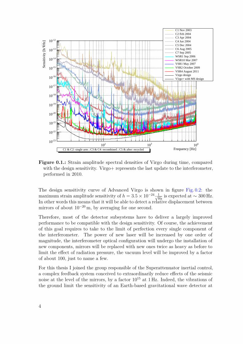
Virgo is a 3 km-long laser Michelson interferometer located in Italy, whose aim is thedirect observation of gravitational wave, in frequency range extended from 10Hz to10 kHz. It acquired data from 2007 up to 2011. As shown in Fig. 0.1, the sensitivityof the experiment has changed during the years, up to reach in 2011 the designspecs with the update named Virgo+: the maximum strain amplitude sensitivitywas h = 4× 10−23 1√

Hz at 300Hz. According to the project, in this final configurationit was supposed to detect a few events per year, but no evidence of gravitationalwave has been found in data analyses so far.

The absence of events is likely due to an overestimation of rates in the initial design,primarily because of a bad knowledge of some stellar parameters. The realistic rate ofevents detectable by Virgo in its initial design, updated to the most recent hypothesisin stellar field, is

Rre ∼ 0.03 yr−1 (0.1)

mostly due to neutron stars coalescence. [1]

It is clear that in these conditions is very difficult to detect something. Because of it,a significant upgrade is in progress at Virgo; this will lead to a new generation ofgravitational wave antennas: Advanced Virgo (AdV). Also LIGO, the other mainexperiment in the gravitational wave field, is undergoing a similar upgrade.

The aim of Advanced Virgo is to achieve a sensitivity that is an improvement onthe original Virgo by one order of magnitude in sensitivity, which corresponds to anincrease of the detection rate by three orders of magnitude. According to a realisticestimation of the binary system coalescence rates in the universe (the same used inequation 0.1), this upgrade would allow to see [1]

Rre ∼ 70 yr−1 (0.2)

3

Frequency [Hz]

210 310 410

]H

zSe

nsiti

vity

[h/

-2310

-2210

-2110

-2010

-1910

-1810

-1710

-1610

-1510

-1410

-1310

-1210

C1 Nov 2003C2 Feb 2004C3 Apr 2004C4 Jun 2004C5 Dec 2004C6 Aug 2005C7 Sep 2005WSR1 Sep 2006WSR10 Mar 2007VSR1 May 2007VSR2 October 2009VSR4 August 2011Virgo designVirgo+ with MS design

C1 & C2: single arm ; C3 & C4: recombined ; C5 & after: recycled

Figure 0.1.: Strain amplitude spectral densities of Virgo during time, comparedwith the design sensitivity. Virgo+ represents the last update to the interferometer,performed in 2010.

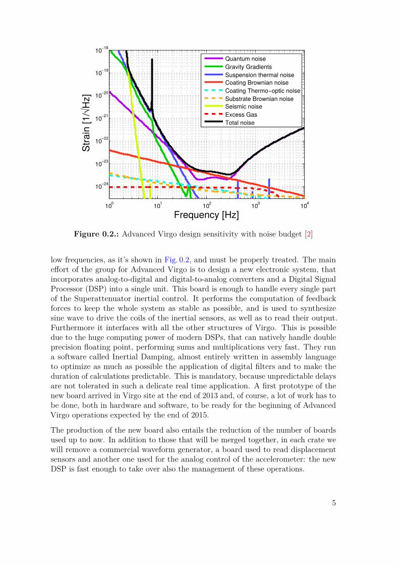
The design sensitivity curve of Advanced Virgo is shown in figure Fig. 0.2: themaximum strain amplitude sensitivity of h = 3.5× 10−24 1√

Hz is expected at ∼ 300Hz.In other words this means that it will be able to detect a relative displacement betweenmirrors of about 10−20 m, by averaging for one second.

Therefore, most of the detector subsystems have to deliver a largely improvedperformance to be compatible with the design sensitivity. Of course, the achievementof this goal requires to take to the limit of perfection every single component ofthe interferometer. The power of new laser will be increased by one order ofmagnitude, the interferometer optical configuration will undergo the installation ofnew components, mirrors will be replaced with new ones twice as heavy as before tolimit the effect of radiation pressure, the vacuum level will be improved by a factorof about 100, just to name a few.

For this thesis I joined the group responsible of the Superattenuator inertial control,a complex feedback system conceived to extraordinarily reduce effects of the seismicnoise at the level of the mirrors, by a factor 1015 at 1Hz. Indeed, the vibrations ofthe ground limit the sensitivity of an Earth-based gravitational wave detector at

4

100 101 102 103 104

10−24

10−23

10−22

10−21

10−20

10−19

10−18

Frequency [Hz]

Stra

in [1

/√H

z]

Quantum noiseGravity GradientsSuspension thermal noiseCoating Brownian noiseCoating Thermo−optic noiseSubstrate Brownian noiseSeismic noiseExcess GasTotal noise

Figure 0.2.: Advanced Virgo design sensitivity with noise budget [2]

low frequencies, as it’s shown in Fig. 0.2, and must be properly treated. The maineffort of the group for Advanced Virgo is to design a new electronic system, thatincorporates analog-to-digital and digital-to-analog converters and a Digital SignalProcessor (DSP) into a single unit. This board is enough to handle every single partof the Superattenuator inertial control. It performs the computation of feedbackforces to keep the whole system as stable as possible, and is used to synthesizesine wave to drive the coils of the inertial sensors, as well as to read their output.Furthermore it interfaces with all the other structures of Virgo. This is possibledue to the huge computing power of modern DSPs, that can natively handle doubleprecision floating point, performing sums and multiplications very fast. They runa software called Inertial Damping, almost entirely written in assembly languageto optimize as much as possible the application of digital filters and to make theduration of calculations predictable. This is mandatory, because unpredictable delaysare not tolerated in such a delicate real time application. A first prototype of thenew board arrived in Virgo site at the end of 2013 and, of course, a lot of work has tobe done, both in hardware and software, to be ready for the beginning of AdvancedVirgo operations expected by the end of 2015.

The production of the new board also entails the reduction of the number of boardsused up to now. In addition to those that will be merged together, in each crate wewill remove a commercial waveform generator, a board used to read displacementsensors and another one used for the analog control of the accelerometer: the newDSP is fast enough to take over also the management of these operations.

5

The Part I of this thesis contains an introduction on the search for gravitationalwaves, from the theoretical background to the possible sources.In the Part II, I study the horizontal accelerometers, feedback-controlled sensors usedin the Superattenuator inertial control to measure the seismic noise in the frequencyband from DC to 100Hz. I analyze their operating principles and the typical signalthat they might measure. Then, exploiting the performances of the new board, Idesign a new control system for the accelerometers, exploiting the properties of acritically damped harmonic oscillatorThe implementation of this system is presented in the Part III of the thesis, togetherwith its noise budget: we see how this new control system increase the sensitivity ofthe experiment of almost one order of magnitude. It contains also the descriptionof an algorithm, implemented in the new electronics, that allows to maximize thesignal-to-noise ratio of the measurement of displacement using a Linear VariableDifferential Transformer (LVDT), a displacement sensor widely used in Virgo.

6

Part I.

Gravitational Waves

7

1A Little of Theory

1.1. An Introduction to General Relativity

The gravitational force dominates the universe on the large scale, binding matterinto stars, stars into galaxies, and galaxies into cluster of galaxies. The classic theoryof gravitation is based on Newton’s law of gravity which states that who masses m1and m2 separated by a distance r feel a mutual gravitational attraction

F = −Gm1m2

r2 (1.1)

where G is a constant of proportionality called “universal gravitational constant”;its value is G = 6.67384(80) × 10−11 m3 kg−1 s−2. [3] This equation describes themotion of the planets around the Sun with great accuracy. However, there are severalfeatures that cannot be explained by the Newton’s law. The most significant one isa tiny component in the precession of the perihelion of the orbit of Mercury. Themain problem is that equation 1.1 is time independent, which would mean that thegravitational force could act instantaneously at all distances. Such behavior is inflat contradiction to the “Special Theory of Relativity” (SR), which requires that nosignal should travel faster than the speed of light c. [4]The problem is shared with electromagnetism and Coulomb’s law: in this case it wassolved with Maxwell’s equations, witch are consistent with SR.In 1916 Albert Einstein published his geometric theory of gravitation, called “GeneralTheory of Relativity” or “General Relativity” (GR), that is a description of gravitationconsistent with special relativity.

1.1.1. The Principle of Equivalence

General relativity is based on the Principle of Equivalence. This establishes theequality of gravitational and inertial mass, demonstrated at first by Galileo and

9

Chapter 1 A Little of Theory

Newton. Einstein interpreted this result to postulate the “weak equivalence principle”:the motion of a neutral test body released at a given point in space-time is independentof its composition. [4]Furthermore, Einstein reflected that, as a consequence, no external static homoge-neous gravitational field could be detected in a freely falling elevator, because theobservers, their test bodies, and the elevator itself would respond to the field withthe same acceleration. Although inertial forces do not exactly cancel gravitationalforces for freely falling systems in an inhomogeneous or time-dependent gravitationalfield, we can still expect an approximate cancellation if we restrict our attention tosuch a small region of space and time that the field changes very little over the region.Therefore, the “strong equivalence principle” was postulated by Einstein and it statesthat at every space-time point in an arbitrary gravitational field is possible to choosea “locally inertial coordinate system” such that, within a sufficiently small regionof the point in question, the laws of nature take the same form as in unacceleratedCartesian coordinate systems in the absence of gravitation. [5]

1.1.2. General Relativity and Einstein’s Field Equations

According to General relativity, the universe consists of an active space-time contin-uum that is distorted by matter and energy passing through it.A first effect predicted by general relativity was detected by Arthur Stanley Eddingtonin 1919. The theory suggest that starlight which passes the limb of the Sun on itsway to the Earth should be deflected by 1.750′′. Eddington organized an expeditionto the Island of Príncipe (São Tomé and Príncipe) which photographed the star fieldaround the Sun during a solar eclipse occurred on May 29. When comparison wasmade with night photographs of the same star field, the predicted general relativisticdeflection was confirmed. [4]Since that day the predictions of general relativity have been confirmed in allobservations and experiments up to now. Among the other results, in the limit oflow velocities and small gravitational effects, GR reduces to Newton’s law with smallcorrections: in the case of Mercury, these corrections account precisely for the smallresidual advance of perihelion.GR allows to describe the curvature of space-time, as directly related to the energyand momentum of whatever matter and radiation are present. The relation isspecified by the Einstein field equations, a set of 10 partial differential equations:

Rµν −12gµνR− λgµν = 8πGTµν (1.2)

gµν is the metric tensor, that contains information about the intensity of the grav-itational field. Rµν represent the curvature of the space-time and contains secondderivatives of gµν , while R = gµνRµν is called scalar curvature. λ was introduced

10

1.2 Gravitational radiation

by Einstein and is called the cosmological constant: for some reasons it has tobe very small and, four our purposes, we can assume λ = 0. Finally, Tµν is theenergy–momentum tensor and contains the distribution of energy and momentum inthe space-time.

1.2. Gravitational radiation

There ares many similarities between gravitation and electromagnetism. It shouldtherefore come as no surprise that Einstein’s equations, like Maxwell equations, haveradiative solutions.We know that electromagnetic propagation is described by d’Alembert equations(c = 1)

Aµ = Jµ/ε0 (1.3)

deriving from Maxwell’s equation, where Aµ = (φ,A) describes the electromagneticpotentials and Jµ = (ρ, j) describes the source of the field. [6] A particular solutionto this equation is represented by the retarded potentials:

Aµ (x, t) = 14πε0

ˆd3x′

Jµ (x′, t− |x′ − x|)|x′ − x|

(1.4)

They show that the state of the field in a certain point of the space-time dependson that of the source at a previous time t− |x′ − x|: the information propagates atspeed c into the electromagnetic waves.The derivation of gravitational radiation from Einstein’s field equations 1.2 is morecomplicated than that of electromagnetic radiation from Maxwell’s equations, dueto the nonlinearity of the first. Maxwell’s equations are linear because the electro-magnetic field does not itself carry charge; on the other hand, we may say that anygravitational wave is itself a distribution of energy and momentum that contributesto the gravitational field of the wave: it is impossible to separate the contributionsof gravitational waves to the curvature from the contributions of the Earth, the Sun,the galaxy, or anything else. Thus, there is no way to find general radiative solutionsof the exact Einstein’s equations.Here we present only the weak-field radiative solutions, which describe waves carryingnot enough energy to affect their own propagation.If we suppose to be far from the source of the fields, the space-time will be nearlyflat and the metric will be close to the Minkowski metric ηµν :

gµν = ηµν + hµν (1.5)

with |hµν | 1. Now Einstein field equations 1.2 can be written to first order in h,

R(1)µν = −8πGSµν (1.6)

11

Chapter 1 A Little of Theory

with

Rµν ' R(1)µν ≡

12

(hµν −

∂2

∂xλ∂xµhλν −

∂2

∂xλ∂xνhλµ + ∂2

∂xµ∂xνhλλ

)

and

Sµν ≡ Tµν −12ηµνT

λλ

We can also perform a further simplification to this equations and, in some steps,write equations 1.6 as

hµν = −16πGSµν (1.7)

These equations are actually very similar to 1.3 and naturally we can write retardedsolutions

hµν (x, t) = −4Gˆd3x′

Sµν (x′, t− |x′ − x|)|x′ − x|

(1.8)

These solutions describe the physical phenomenon of the gravitational waves producedby the source Sµν . They are transverse waves traveling with the same finite speedof propagation c of the electromagnetic waves and the same intensity decrease asfunction of distance from the source.Far from the source, as |x′ − x| → ∞, the retarded solution approaches a planewave, and the equations 1.7 are reduced to the homogeneous ones, hµν = 0. Here,a solution is

hµν = eµν exp(ikλx

λ)

+ e∗µν exp(−ikλxλ

)(1.9)

with

kµkµ = 0 (1.10)

and

kµeµν = 1

2kνeµµ (1.11)

eµν = eνµ is a 4x4 symmetric tensor and is called the polarization tensor. In general,a 4x4 matrix have 10 independent components; the gauge invariance 1.11 reducethem to only 6, but it can be shown that of these six there are only two physicallysignificant degrees of freedom, i.e. only two independent physical polarizations. [5]The commonly used couple of independent polarization is

e+µν =

0 0 0 00 1 0 00 0 −1 00 0 0 0

and e×µν =

0 0 0 00 0 1 00 1 0 00 0 0 0

(1.12)

12

1.3 The Effects of Gravitational Waves

and it forms a basis for the polarization space. The two elements are pronouncedrespectively plus and cross polarizations. We can obtain any other polarization (forexample the circular polarizations) by a suitable linear superposition of these two.

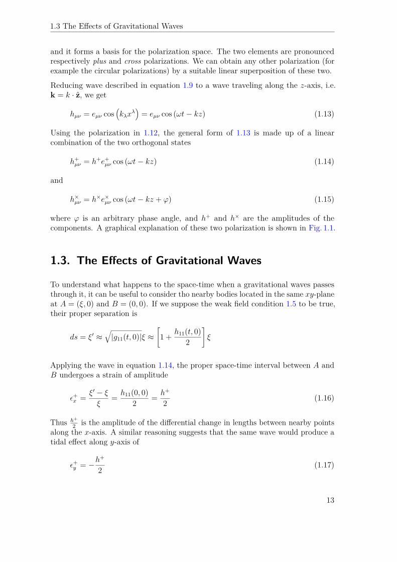
Reducing wave described in equation 1.9 to a wave traveling along the z-axis, i.e.k = k · z, we get

hµν = eµν cos(kλx

λ)

= eµν cos (ωt− kz) (1.13)

Using the polarization in 1.12, the general form of 1.13 is made up of a linearcombination of the two orthogonal states

h+µν = h+e+

µν cos (ωt− kz) (1.14)

and

h×µν = h×e×µν cos (ωt− kz + ϕ) (1.15)

where ϕ is an arbitrary phase angle, and h+ and h× are the amplitudes of thecomponents. A graphical explanation of these two polarization is shown in Fig. 1.1.

1.3. The Effects of Gravitational Waves

To understand what happens to the space-time when a gravitational waves passesthrough it, it can be useful to consider tho nearby bodies located in the same xy-planeat A = (ξ, 0) and B = (0, 0). If we suppose the weak field condition 1.5 to be true,their proper separation is

ds = ξ′ ≈√|g11(t, 0)|ξ ≈

[1 + h11(t, 0)

2

]ξ

Applying the wave in equation 1.14, the proper space-time interval between A andB undergoes a strain of amplitude

ε+x = ξ′ − ξξ

= h11(0, 0)2 = h+

2 (1.16)

Thus h+

2 is the amplitude of the differential change in lengths between nearby pointsalong the x-axis. A similar reasoning suggests that the same wave would produce atidal effect along y-axis of

ε+y = −h+

2 (1.17)

13

Chapter 1 A Little of Theory

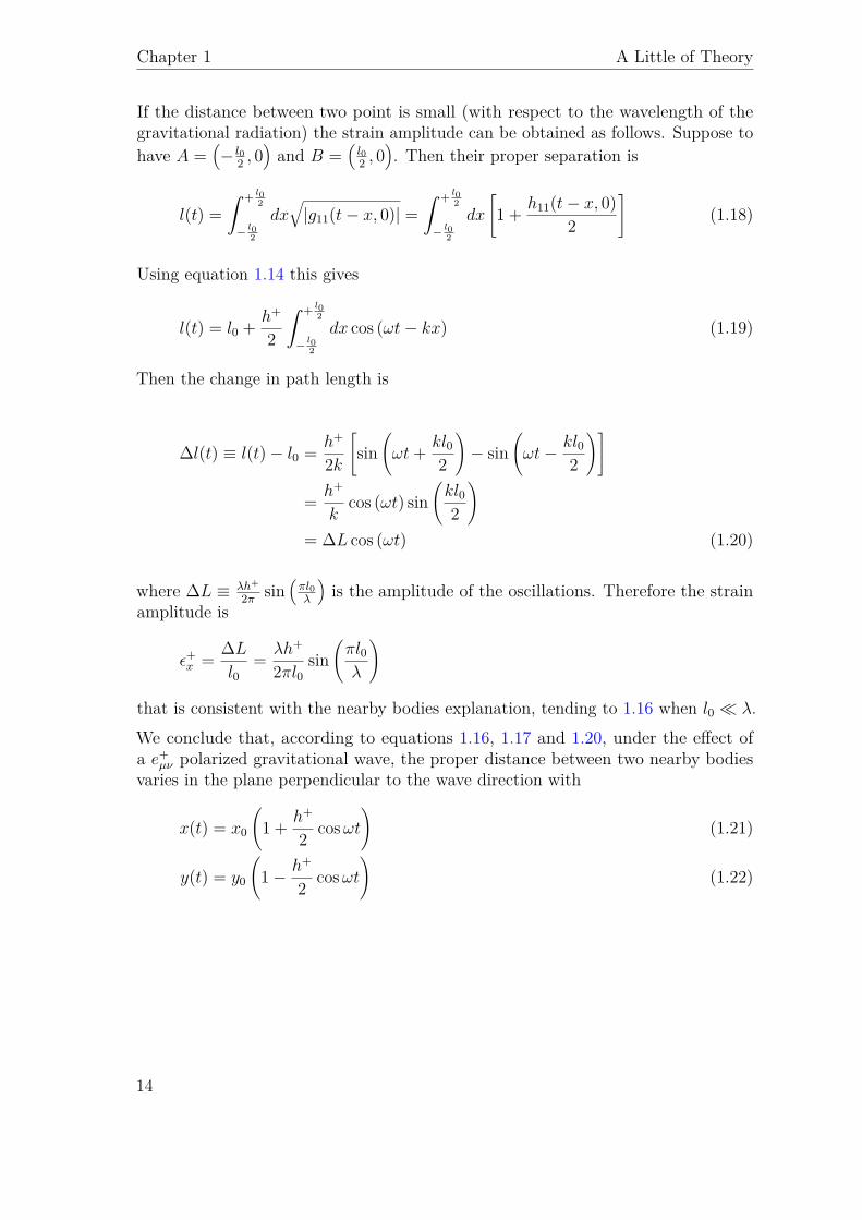
If the distance between two point is small (with respect to the wavelength of thegravitational radiation) the strain amplitude can be obtained as follows. Suppose tohave A =

(− l0

2 , 0)and B =

(l02 , 0

). Then their proper separation is

l(t) =ˆ + l0

2

− l02

dx√|g11(t− x, 0)| =

ˆ + l02

− l02

dx

[1 + h11(t− x, 0)

2

](1.18)

Using equation 1.14 this gives

l(t) = l0 + h+

2

ˆ + l02

− l02

dx cos (ωt− kx) (1.19)

Then the change in path length is

∆l(t) ≡ l(t)− l0 = h+

2k

[sin

(ωt+ kl0

2

)− sin

(ωt− kl0

2

)]

= h+

kcos (ωt) sin

(kl02

)= ∆L cos (ωt) (1.20)

where ∆L ≡ λh+

2π sin(πl0λ

)is the amplitude of the oscillations. Therefore the strain

amplitude is

ε+x = ∆Ll0

= λh+

2πl0sin

(πl0λ

)

that is consistent with the nearby bodies explanation, tending to 1.16 when l0 λ.We conclude that, according to equations 1.16, 1.17 and 1.20, under the effect ofa e+

µν polarized gravitational wave, the proper distance between two nearby bodiesvaries in the plane perpendicular to the wave direction with

x(t) = x0

(1 + h+

2 cosωt)

(1.21)

y(t) = y0

(1− h+

2 cosωt)

(1.22)

14

1.3 The Effects of Gravitational Waves

h+µν = h+e+

µν cos (ωt) h×µν = h×e×µν cos (ωt)

ωt = 0

ωt = π2

ωt = π

ωt = 3π2

ωt = 2π

Figure 1.1.: The effect of gravitational waves in two different polarization (e+µν and

e×µν) on a circle of test masses followed over one cycle. The wave is traveling alongthe z-axis, the paper is the xy-plane at z = 0, and the observer is looking towardsthe source.

15

2The Search for Gravitational Waves

Now that we understand the effects of gravitational waves on the space-time, weneed to look for the sources and to estimate the typical amplitude of their radiationwhen it reach the Earth.

In principle, gravitational waves can experience almost all the familiar peculiaritiesof propagation typical of electromagnetic waves. Nevertheless nobody has so fardetected any direct evidence of gravitational waves.

A direct detection is defined as the measurement of the perturbation h (t) asfunction of the time, while the term indirect detection refers to the observation ofphenomena that suggest the presence of a gravitational radiation, without makingpossible any measurement of its waveform.

Even if, as of 2014, no direct detection of gravitational waves has yet been claimed,there are strong indications that such radiation exists, because at least a pair ofsources may already has been detected.

2.1. The First Indirect Observation: PSR B1913+16

The most famous indirect detection dates back to 1974: it is the binary systemmade by pulsar PSR B1913+16 and another neutron star, orbiting around theircenter of mass. The orbit period is Pb = 7.75 h and the projected orbital velocityis v ∼ c/1000: this suggest that there can be some measurable relativistic effects.Among the best known results are measurement of the general relativistic advanceof periastron at a rate ∼ 35× 103 times that of Mercury in the solar system and,above all, the effect of gravitational radiation damping, causing a measurable rate oforbital decay. [7]

Peters and Matthews [8] showed that, according to general relativity, the resultingrate of change in orbital period, measured in the orbiting system reference frame,

17

Chapter 2 The Search for Gravitational Waves

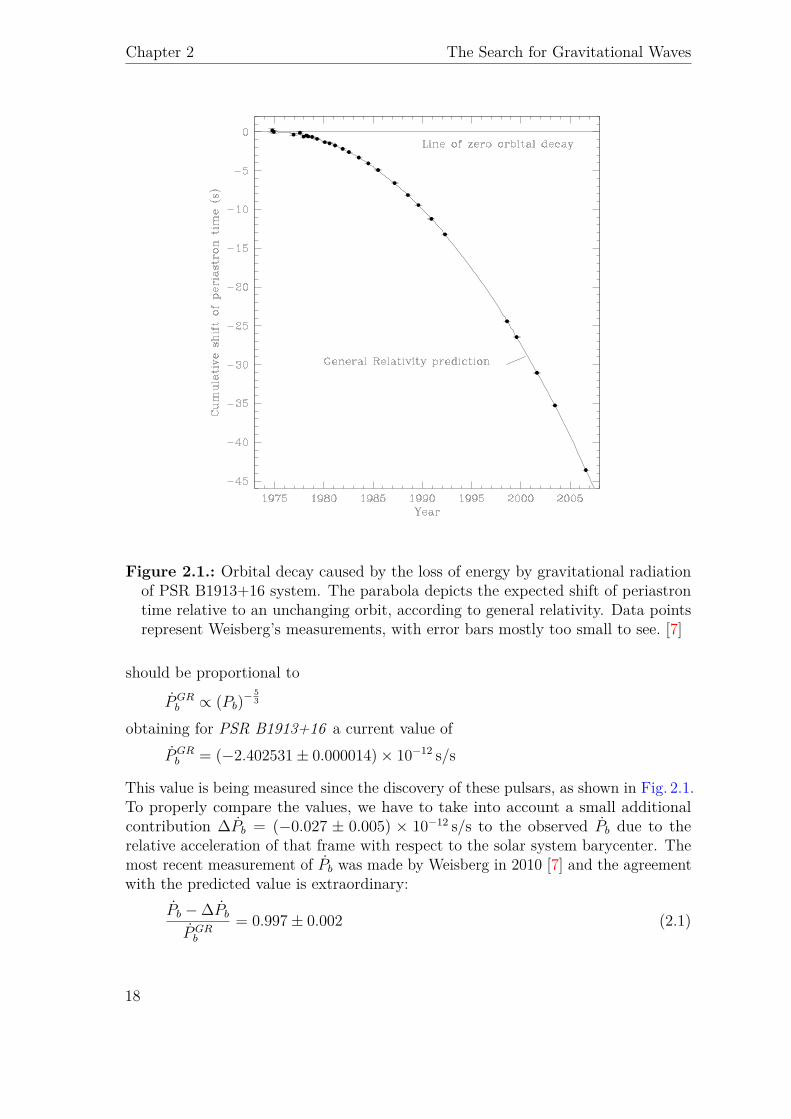
Figure 2.1.: Orbital decay caused by the loss of energy by gravitational radiationof PSR B1913+16 system. The parabola depicts the expected shift of periastrontime relative to an unchanging orbit, according to general relativity. Data pointsrepresent Weisberg’s measurements, with error bars mostly too small to see. [7]

should be proportional to

PGRb ∝ (Pb)−

53

obtaining for PSR B1913+16 a current value ofPGRb = (−2.402531± 0.000014)× 10−12 s/s

This value is being measured since the discovery of these pulsars, as shown in Fig. 2.1.To properly compare the values, we have to take into account a small additionalcontribution ∆Pb = (−0.027 ± 0.005) × 10−12 s/s to the observed Pb due to therelative acceleration of that frame with respect to the solar system barycenter. Themost recent measurement of Pb was made by Weisberg in 2010 [7] and the agreementwith the predicted value is extraordinary:

Pb −∆PbPGRb

= 0.997± 0.002 (2.1)

18

2.2 BICEP2 and Inflationary Gravitational Radiation

This result provides conclusive evidence for the existence of gravitational radiation,as predicted by Einstein’s theory.

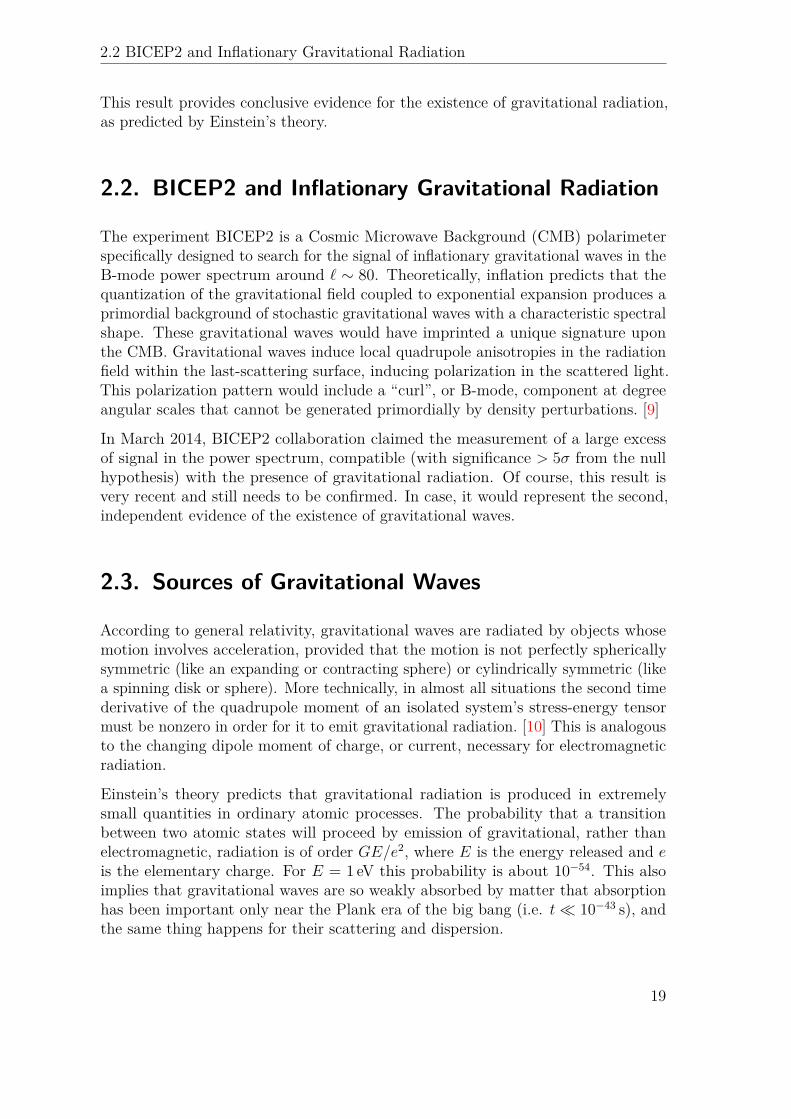
2.2. BICEP2 and Inflationary Gravitational Radiation

The experiment BICEP2 is a Cosmic Microwave Background (CMB) polarimeterspecifically designed to search for the signal of inflationary gravitational waves in theB-mode power spectrum around ` ∼ 80. Theoretically, inflation predicts that thequantization of the gravitational field coupled to exponential expansion produces aprimordial background of stochastic gravitational waves with a characteristic spectralshape. These gravitational waves would have imprinted a unique signature uponthe CMB. Gravitational waves induce local quadrupole anisotropies in the radiationfield within the last-scattering surface, inducing polarization in the scattered light.This polarization pattern would include a “curl”, or B-mode, component at degreeangular scales that cannot be generated primordially by density perturbations. [9]

In March 2014, BICEP2 collaboration claimed the measurement of a large excessof signal in the power spectrum, compatible (with significance > 5σ from the nullhypothesis) with the presence of gravitational radiation. Of course, this result isvery recent and still needs to be confirmed. In case, it would represent the second,independent evidence of the existence of gravitational waves.

2.3. Sources of Gravitational Waves

According to general relativity, gravitational waves are radiated by objects whosemotion involves acceleration, provided that the motion is not perfectly sphericallysymmetric (like an expanding or contracting sphere) or cylindrically symmetric (likea spinning disk or sphere). More technically, in almost all situations the second timederivative of the quadrupole moment of an isolated system’s stress-energy tensormust be nonzero in order for it to emit gravitational radiation. [10] This is analogousto the changing dipole moment of charge, or current, necessary for electromagneticradiation.

Einstein’s theory predicts that gravitational radiation is produced in extremelysmall quantities in ordinary atomic processes. The probability that a transitionbetween two atomic states will proceed by emission of gravitational, rather thanelectromagnetic, radiation is of order GE/e2, where E is the energy released and eis the elementary charge. For E = 1 eV this probability is about 10−54. This alsoimplies that gravitational waves are so weakly absorbed by matter that absorptionhas been important only near the Plank era of the big bang (i.e. t 10−43 s), andthe same thing happens for their scattering and dispersion.

19

Chapter 2 The Search for Gravitational Waves

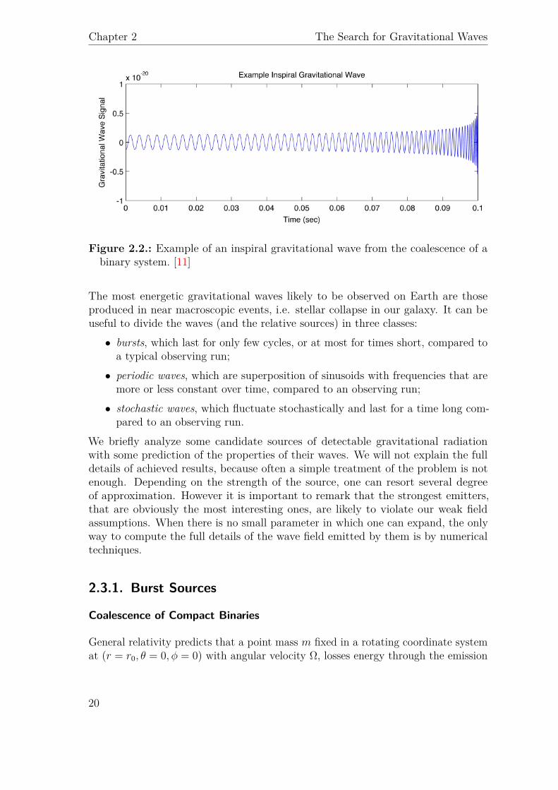
Figure 2.2.: Example of an inspiral gravitational wave from the coalescence of abinary system. [11]

The most energetic gravitational waves likely to be observed on Earth are thoseproduced in near macroscopic events, i.e. stellar collapse in our galaxy. It can beuseful to divide the waves (and the relative sources) in three classes:• bursts, which last for only few cycles, or at most for times short, compared to

a typical observing run;• periodic waves, which are superposition of sinusoids with frequencies that are

more or less constant over time, compared to an observing run;• stochastic waves, which fluctuate stochastically and last for a time long com-

pared to an observing run.We briefly analyze some candidate sources of detectable gravitational radiationwith some prediction of the properties of their waves. We will not explain the fulldetails of achieved results, because often a simple treatment of the problem is notenough. Depending on the strength of the source, one can resort several degreeof approximation. However it is important to remark that the strongest emitters,that are obviously the most interesting ones, are likely to violate our weak fieldassumptions. When there is no small parameter in which one can expand, the onlyway to compute the full details of the wave field emitted by them is by numericaltechniques.

2.3.1. Burst Sources

Coalescence of Compact Binaries

General relativity predicts that a point mass m fixed in a rotating coordinate systemat (r = r0, θ = 0, φ = 0) with angular velocity Ω, losses energy through the emission

20

2.3 Sources of Gravitational Waves

of gravitational radiation at twice the frequency of the orbit, with power

P (2Ω) = 32GΩ6m2r40

5c5 (2.2)

A direct calculation of the power emitted by a planet orbiting around its star suggestthat it is very weak: for example, Jupiter’s loss of energy through gravitationalradiation, because of its orbit around the Sun, is ∼ 5.3 kW. [5]However, this value can be significant if we study the behavior of binary systemof massive stars orbiting around their center of mass, close enough to be driveninto coalescence by gravitational radiation reaction, in a time less than the age ofuniverse. These systems are usually two neutron stars, two black holes, or a neutronstar and a black hole whose orbits have degraded to the point that the two massesare about to coalesce. In this phase the system generates spiral gravitational waves.The binary star system PSR B1913+16 is an example of such a system.As the two masses rotate around each other, their orbital distances decrease andtheir speeds increase: this causes the frequency of the gravitational waves they emitto increase up to f ' 1 kHz (in the most common case of two neutron stars) untilthe two objects definitively merge into one. An example of the expected signal froman event of this kind is shown in Fig. 2.2.The characteristic amplitude of the burst waves at a distance r from the source canbe obtained with this relation:

hc ∼ 10−22(M

M

) 13(

µ

M

) 12(

100Hzfc

) 16(

100MPcr

)(2.3)

where M and µ are respectively the total mass of the system and the reduced mass(expressed in solar masses), and fc is a characteristic frequency of the waves. [10]At present, there are significant uncertainties in the astrophysical rate predictions forcompact binary coalescences. A realistic estimation of double neutron star systemcoalescence rate is ∼ 100Myr−1 for a galaxy similar to Milky Way that correspondsto volumetric rate of ∼ 1Mpc−3 Myr−1. [1] For example, the aforementioned PSRB1913+16 binary system is going to coalesce in ∼ 300Myr.

Supernovae

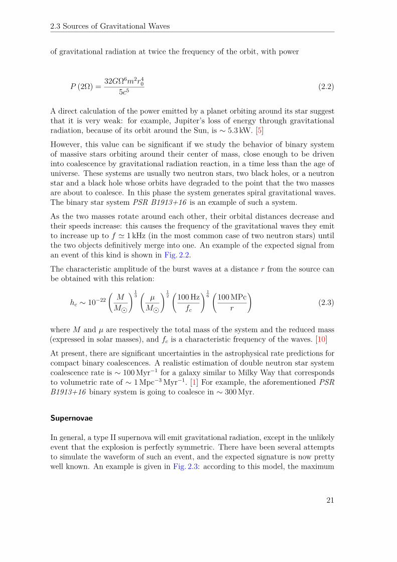
In general, a type II supernova will emit gravitational radiation, except in the unlikelyevent that the explosion is perfectly symmetric. There have been several attemptsto simulate the waveform of such an event, and the expected signature is now prettywell known. An example is given in Fig. 2.3: according to this model, the maximum

21

Chapter 2 The Search for Gravitational Waves

0 20 40 60 80 100 120 140 160 180-20-15-10-50510

h+Dh×D

-20-15-10-50510

t− tbounce [ms]

h +D,h

×D

[cm]

h +D,h

×D

[cm]

Polar Observer

Equatorial Observer

Figure 2.3.: Gravitational wave polarizations h+ and h× (rescaled by distance D)obtained in a simulation (Ott et al., 2013 [12]) as a function of post-bounce timeseen by and observer on the pole (θ = 0, φ = 0; top panel) and on the equator(θ = π/2, φ = 0; bottom panel)

amplitude of waves is expected to be h ≈ 20 cm/D, that correspond to h ≈ 10−22 ata distance D = 10 kpc.A more generic formula to obtain the order of magnitude of h at a distance r fromthe source is

hc ∼ 2.7× 10−20(EGWM

) 12(

1 kHzfc

) 12(

10Mpcr

)(2.4)

where EGW is the energy emitted through gravitational radiation by the supernova,expressed in solar masses, and 200Hz . fc . 10 kHz is the characteristic frequencyof the waves in these events. [10] Its value depends strongly on the asymmetry of theexplosion. Recent simulations indicate an expected value of EGW ∼ 10−8M. [13]

2.3.2. Periodic Sources

Pulsars

Pulsars are highly magnetized, rotating neutron stars. Possible asymmetries in massdistribution lead to the emission of gravitational radiation. The larger are those

22

2.3 Sources of Gravitational Waves

asymmetries and the more rapidly they rotate, the stronger will be the radiation.Due to their high stability, pulsars are hypothesized to emit continuous, narrow-band,quasi-sinusoidal gravitational waves.These sources are expected to produce comparatively weak gravitational waves sincethey evolve over longer periods of time, and are usually less catastrophic than inspiralor burst sources. The characteristic amplitude of these waves, measured at a distancer from the pulsar rotating around z-axis, can be obtained as

hc ∼ 8× 10−20ε

(Izz

1038 kgm2

)(f

1 kHz

)2 (10 kpcr

)(2.5)

with fiducial equatorial gravitational ellipticity ε defined as

ε = Qxx −Qyy

Izz

where Qxx and Qyy are quadrupole moments with respect to x and y axes, and Izz isthe moment of inertia around z-axis. [10]Equation 2.5 leads to expected amplitudes h ∼ 10−24÷25 for the most interestingknown pulsars, in the limit case in which they loss energy only through the emissionof gravitational radiation. Despite the weakness of the waves, in principle the signalcan be seen averaging it over many periods. Actually known pulsars usually haveprecisely determined frequency evolutions and sky-positions making them idealtargets for gravitational wave detectors. If a pulsar is monitored regularly throughelectromagnetic observations it can yield a coherent phase model, which allowsgravitational wave data to be coherently integrated over months or years. [14]

Ordinary Binary Stars

Ordinary binary star systems are the most reliably understood sources of gravitationalwaves. From the measured mass and orbital parameters of a binary and its estimatedistance, one can compute with confidence the details of its waves.Unfortunately, ordinary binaries have orbital periods usually longer than an hour, thatcorrespond to f ∼ 1mHz. Because of seismic noise, detectors in earth laboratoriescannot hope to see waves at such low frequencies.The characteristic amplitude of such waves measured at a distance r from the sourceis

hc ∼ 10−20(M

M

) 23(

µ

M

)(fc

10mHz

) 23 (100 pc

r

)(2.6)

where fc is twice the frequency of the orbit. [10]

23

Chapter 2 The Search for Gravitational Waves

2.3.3. Stochastic Background

The discovery of the CMB in 1964 suggests that there can be a gravitational analogous.This type of background is called Stochastic Gravitational-Wave Background (SGWB)and could be the result of processes that took place very shortly after the Big Bang,but since we know very little about the state of the universe at that time, it is hardto make predictions.While the evolution of the universe following the Big Bang Nucleosynthesis (BBN) iswell understood, there is little observational data probing the evolution prior to BBN,when the universe was less than one minute old. The gravitational wave spectrumshould carry information about exactly this epoch of the universe evolution.Nevertheless, such a background might also arise from processes that take place fairlyrecently (within the past several billion years) and this more recent contributionmight overwhelm the parts of the background which contain information about thestate of the early universe. [15]The spectral properties of the stochastic background are characterized by the densityparameter ΩGW (ν), a dimensionless value defined as

ΩGW (ν) = 1ρcr

dρGWd ln ν

where ρcr is the critical energy-density required to just close the universe and dρGWis the energy density of gravitational radiation contained in frequency range ν toν+dν. [16] This parameter is one of the contribute to the sum in Friedmann equation(assuming the universe to be flat)∑

i

Ωi + ΩΛ = 1 (2.7)

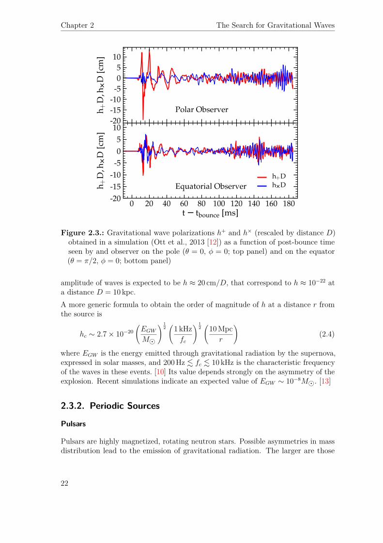
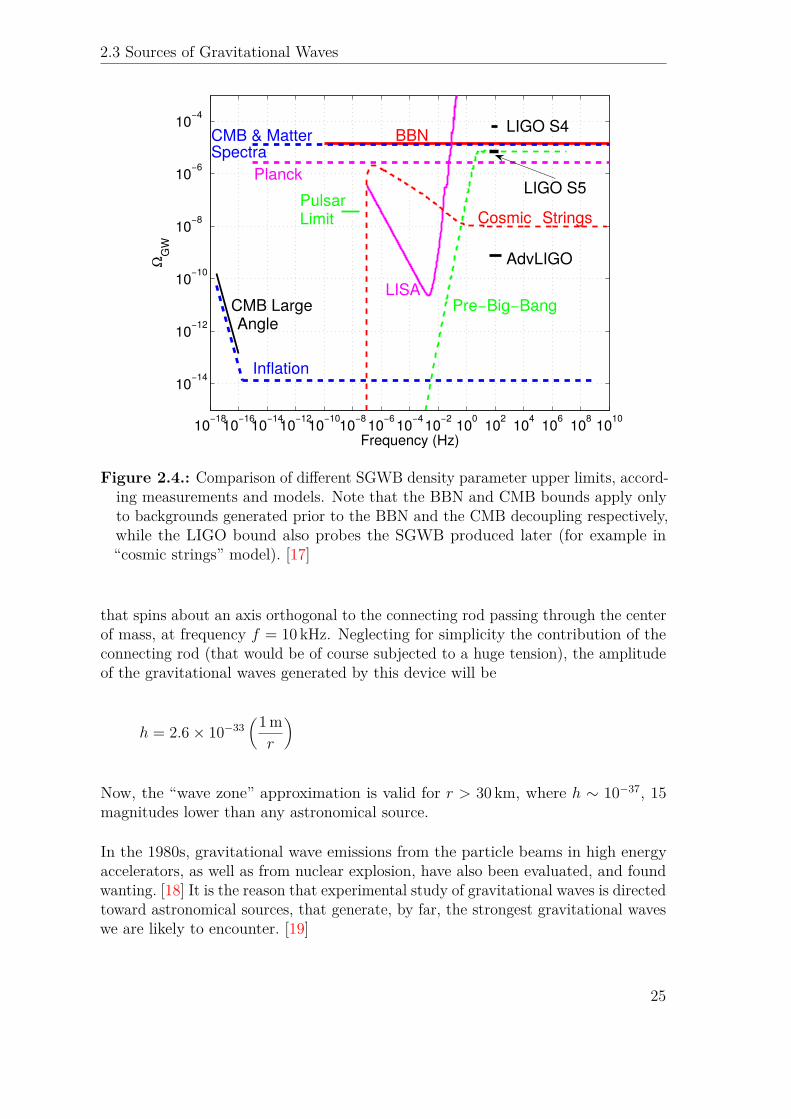
where Ωi are the density parameters for the various matter species and ΩΛ for thecosmological constant.It is hard to make a theoretical estimation of this density parameter, but an upperlimit can be obtained from direct and indirect measurements. If we assume ΩGW (ν) tobe constant, i.e. a frequency independent gravitational wave spectrum, experimentalresults of LIGO and Virgo give an upper limit (95% CL) of its value: ΩGW <6.9× 10−6. Other upper limits achievable with several theoretical models and someexperiments are presented in Fig. 2.4.The network of advanced detectors actually under development will be able to probethe isotropic SGWB at the level of ΩGW ∼ 10−9 or smaller. [17]

2.3.4. The Impracticality of Artificial Sources

No artificial generator of gravitational waves seems practicable. For example, considera dumbbell consisting of two masses of 103 kg each, at either ends of a 2m-long rod,

24

2.3 Sources of Gravitational Waves

10−1810−1610−1410−1210−1010−8 10−6 10−4 10−2 100 102 104 106 108 1010

10−14

10−12

10−10

10−8

10−6

10−4

CMB LargeAngle

PulsarLimit

LIGO S4

AdvLIGO

BBNCMB & MatterSpectra

Planck

Inflation

LISAPre−Big−Bang

Cosmic Strings

LIGO S5

Frequency (Hz)

ΩG

W

Figure 2.4.: Comparison of different SGWB density parameter upper limits, accord-ing measurements and models. Note that the BBN and CMB bounds apply onlyto backgrounds generated prior to the BBN and the CMB decoupling respectively,while the LIGO bound also probes the SGWB produced later (for example in“cosmic strings” model). [17]

that spins about an axis orthogonal to the connecting rod passing through the centerof mass, at frequency f = 10 kHz. Neglecting for simplicity the contribution of theconnecting rod (that would be of course subjected to a huge tension), the amplitudeof the gravitational waves generated by this device will be

h = 2.6× 10−33(1mr

)

Now, the “wave zone” approximation is valid for r > 30 km, where h ∼ 10−37, 15magnitudes lower than any astronomical source.

In the 1980s, gravitational wave emissions from the particle beams in high energyaccelerators, as well as from nuclear explosion, have also been evaluated, and foundwanting. [18] It is the reason that experimental study of gravitational waves is directedtoward astronomical sources, that generate, by far, the strongest gravitational waveswe are likely to encounter. [19]

25

Chapter 2 The Search for Gravitational Waves

2.4. Detectors of Gravitational Waves

A gravitational-wave detector is any device designed to measure gravitational waves.Since the 1960s gravitational-wave detectors have been built and constantly improved.Some types of detectors, both proposed and realized, are here grouped according totheir bandwidth:• High frequency detectors: Weber bar, interferometer, super-fluid interferometers

and superconducting circuits.• Low frequency detectors: Doppler tracking of spacecraft, interferometer in

space, Earth’s normal modes, Sun’s normal modes, vibration of blocks of theEarth’s crust, skyhook.• Very low frequency detectors: pulsar timing, timing of orbital motions, anisotropies

in the temperature of the cosmic microwave radiation (indirect detection).Note that, due to the stochastic movements of the ground, only high-frequencydetectors can be earth-based. The most common types of detectors are resonantbars (aka Weber bars) and interferometers.

2.4.1. Weber Bars

Resonant bars have represented the first type of gravitational-wave detector. Alarge, solid bar of metal isolated from outside vibrations, designed to detect theexpected wave motion is called a Weber bar. Strains in space due to an incidentgravitational wave excite the resonant frequency of the bar, and these vibrationscould be amplified to detectable levels. When a burst of gravitational waves hitsand excites the oscillator, this will vibrate for a time span much longer than theduration of the burst (typically 1ms), thus allowing the extraction of the signal fromthe detector noise. [20] Their sensitivity is limited to a very narrow bandwidth, sothat Weber bars are not sensitive enough to detect anything but extremely powerfulgravitational waves.For example, AURIGA (Antenna Ultracriogenica Risonante per l’Indagine Gravita-zionale Astronomica) is an ultracryogenic resonant bar gravitational wave detectorin Italy. It is located at the Laboratori Nazionali di Legnaro of the INFN. Nowadays,the other working experiments are MiniGrail (Netherlands) and Mario Schenberg(Brazil).

2.4.2. Interferometers

Interferometric detectors are the most interesting devices ever conceived to detectgravitational waves. Indeed we can determine the distance between two test masses(nothing more than mirrors) by measuring the round trip travel time of light beams

26

2.4 Detectors of Gravitational Waves

sent over large distances, and thus it is natural to aim at Michelson interferometer.The key difference with the 1887 interferometer is that here we need not connectthe mirrors in a single rigid structure, but each mass is left in free fall, so that itresponds in a indepentend way to gravitational effects.

We can calculate the time that it takes to that ray to travel in each arm of ourinterferometer, when it is crossed by a gravitational wave. In equations 1.21 and1.22 We have already seen the effect on the distance between two points; in aMichelson interferometer the arms are orthogonal and their lengths L equal eachother (L = x0 = y0), so that the relative variation

∆L (t) = 2 [x (t)− y (t)] = 2L · h+ cosωt= 2L · h (t) (2.8)

where the additional factor 2 takes into account for the round trip in the interferometer,and h (t) = h+ cosωt. Remembering that for light ds2 = 0, this correspond to adifference in time of arrival

∆τ (t) = ∆L (t)c

= 2Lch (t)

= τ0 · h (t) (2.9)

where τ0 is the travel time in absence of gravitational radiation. Corrections tothis due to the effect of the gravitational wave itself are negligible. [19] We can alsoexpress 2.9 as a phase shift:

∆ϕ (t) = 2πcλL

τ0 · h (t) (2.10)

where λL is the wavelength of the light used in the interferometer. It is clear that theeffect is directly proportional to h: this immediately says that the longer the opticalpath in the apparatus, the larger will be the phase shift due to the gravitationalwave.

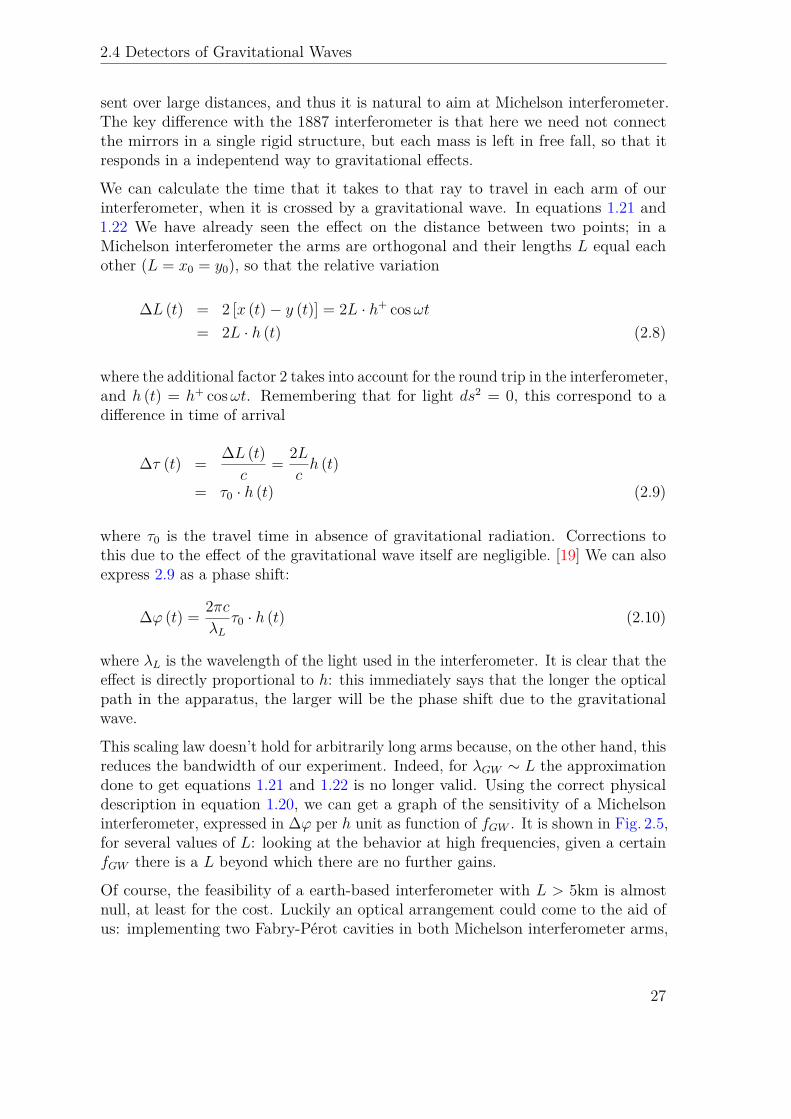
This scaling law doesn’t hold for arbitrarily long arms because, on the other hand, thisreduces the bandwidth of our experiment. Indeed, for λGW ∼ L the approximationdone to get equations 1.21 and 1.22 is no longer valid. Using the correct physicaldescription in equation 1.20, we can get a graph of the sensitivity of a Michelsoninterferometer, expressed in ∆ϕ per h unit as function of fGW . It is shown in Fig. 2.5,for several values of L: looking at the behavior at high frequencies, given a certainfGW there is a L beyond which there are no further gains.

Of course, the feasibility of a earth-based interferometer with L > 5km is almostnull, at least for the cost. Luckily an optical arrangement could come to the aid ofus: implementing two Fabry-Pérot cavities in both Michelson interferometer arms,

27

Chapter 2 The Search for Gravitational Waves

10−2

10−1

100

101

102

103

104

107

108

109

1010

1011

1012

1013

Gravitational wave frequency (Hz)

Phase

shift(∆

ϕ/h)

Sensitivity of Michelson interferometer

Michelson 3kmMichelson 100kmMichelson 400kmFabry-Perot 3km (F = 150)

Figure 2.5.: Phase shift per h unit(

∆ϕh

)in a L-long Michelson interferometer as

function of fGW . The light has wavelength λL = 1.064 µm. The peaks correspond toλGW = L/n with n ∈ N, when a whole numbers of waves fit into the interferometer,canceling the effects. [21]

we achieve the same performance of a longer interferometer. In brief, photons aretrapped in the cavities for an average time

τs = 2Lc

Fπ

(2.11)

or, in other words, travel F/π times through the cavity before to come out. Thequantity F is a quality index of the cavity, and it is called finesse. From Fig. 2.5, itis shown as the sensitivity of a 3km long interferometer with F = 150 Fabry-Pérotcavities is roughly equivalent to a 400 km standard interferometer.So far there have been at least 4 working interferometric detectors: LIGO (USA,3 detectors in 2 sites), VIRGO (Italy), GEO 600 (Germany), and TAMA 300(Japan). An interesting experiment is eLISA: it will be the first dedicated space-basedgravitational wave detector, using laser interferometry to monitor the fluctuations inthe relative distances between three spacecrafts, arranged in an equilateral trianglewith 109 m arms (almost the diameter of the Sun).

28

Part II.

Accelerometer Control

29

3An Introduction to Control Theory

Feedback is a central feature of life. The process of feedback governs how we grow,respond to stress and challenge, and regulate factors such as body temperature,blood pressure and cholesterol level. The mechanisms operate at every level, from theinteraction of proteins in cells to the interaction of organisms in complex ecologies.Nowadays feedback controls are essential in any field of science and engineering. AlsoVirgo contains several control systems. The highest level is represented by a closedloop control system that is used both during the lock acquisition of the interferometerand the steady state (science mode) operations. It must be capable of the maintainingthe interferometer controlled at the design sensitivity with good stability and dutycycle. It controls the position of the optical elements of the interferometer, which inturn are controlled by other local closed loop control systems. Also further levels ofcontrol exist: for example, the accelerometers used in Virgo seismic isolation systemuse a feedback control to work to the best of their abilities.In this chapter we introduce some basic concepts of control theory applied tocontinuous-time systems. Later, these basis will be extended to discrete-time systems.

3.1. Linear Time-Invariant Systems

It is possible to distinguish two main classes of systems:• linear systems• nonlinear systems

A system is called linear if the superposition principle applies. The superpositionprinciple states that the net response at a given place and time, caused by two ormore stimuli, is the sum of the responses which would have been caused by eachstimulus individually. Hence, for a linear system, the response to several inputscan be calculated by treating one input at a time and adding the results. It is this

31

Chapter 3 An Introduction to Control Theory

principle that allows one to build up complicated solutions to the linear differentialequation from simple solutions. In an experimental investigation of a dynamic system,if cause and effect are proportional, thus implying that the superposition principleholds, then the system can be considered linear.

A differential equation is linear if its coefficients are constants or functions only of theindependent variable. Dynamic systems that are composed of linear time-invariantlumped-parameter components may be described by linear time-invariant differentialequations - i.e. constant-coefficient differential equations. Such systems are calledLinear Time-Invariant systems (or LTI systems). On the other hand, systems thatare represented by differential equations whose coefficients are functions of time arecalled linear time-variant systems. [22]

Eventually, systems that does not satisfy the superposition principle, which meansthat the output is not directly proportional to the input, are called nonlinear systems.

3.2. Transfer Functions

In control theory, functions called transfer functions are commonly used to charac-terize the input-output relationships of components or systems that can be describedby linear, time-invariant, differential equations. They are defined as the ratio of theLaplace transform of the output (response function) to the Laplace transform of theinput (driving function) under the assumption that all initial conditions are zero.Laplace transform L [·] and its inverse transform L−1 [·] are defined in Appendix A,together with some properties.

Consider the linear time-invariant system defined by the following differential equation:

an(n)y + an−1

(n−1)y + . . .+ a1y + a0y = bm

(m)x + bm−1

(m−1)x + . . .+ b1x+ b0x (3.1)

where y = y (t) is the output of the system and x = x (t) is the input. The transferfunction G (s) of this system is

G (s) = Y (s)X (s) = bms

m + bm−1sm−1 + . . .+ b1s+ b0

ansn + an−1sn−1 + . . .+ a1s+ a0=

m∑i=0bis

i

n∑j=0ajsj

(3.2)

where X (s) = L [x] and Y (s) = L [y] .

A common notation convention, where lower case letters denote signals and capitalletters their Laplace transforms, is used in the thesis. Furthermore, in order toobtain a lighter notation, the explicit dependence of signals on time t will be usuallyomitted, as also the explicit dependence of their Laplace transforms on s.

32

3.2 Transfer Functions

By using the concept of transfer function, it is possible to represent system dynamicsby algebraic equations in s. If the highest power of s in the denominator of thetransfer function is equal to n, the system is called an nth-order system.

It follows from equation 3.2 that the output can be written as

Y = G ·X (3.3)

From convolution theorem we know that

x ∗ y = L−1 [L [x] · L [y]] = L−1 [X · Y ] (3.4)

Applying the inverse Laplace transform to both sides of 3.3, and using 3.4, we findthe relation between input and output in time domain

y (t) =ˆ +∞

−∞x (τ) g (t− τ) dτ

=ˆ +∞

−∞g (τ)x (t− τ) dτ (3.5)

where g (t) = L−1 [G (s)], and both g (t) and x (t) are 0 for t < 0. The functiong (t) represents the impulse response of the system: applying an unit-impulse inputx (t) = δ (t) to the system indeed, equation 3.5 states that y (t) = g (t). Similarly,G (s) is the unit-impulse response in frequency domain.

If the transfer function of a system is unknown, it is hence possible to obtain completeinformation about the dynamic characteristics of the system by exciting its inputwith an impulse or with white noise, and measuring the response at the output. TheLaplace transform of the output is the transfer function of that system, and it givesa full description of the dynamic characteristics of the system. Of course this methodcan be used also to check the goodness of a mathematical model of the system. [22]

Also other forms of mathematical models exist. For example, often it is advantageousto use state-space representation: it consists of 4 matrices (A, B, C and D) that,if u is the input vector, y is the output vector and x is the state vector, representthe state in this form:

x (t) = A (t)x (t) +B (t)u (t)y (t) = C (t)x (t) +D (t)u (t)

Unlike the frequency domain approach, the use of the state space representationis not limited to systems with linear components and zero initial conditions. Thisrepresentation is extensively used in Virgo control systems.

33

Chapter 3 An Introduction to Control Theory

G HX U Y

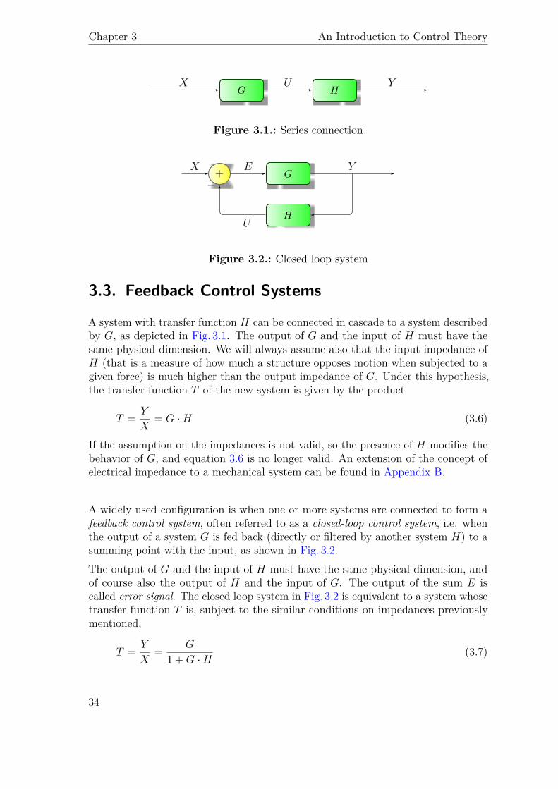
Figure 3.1.: Series connection

+ G

H

X E Y

−

U

Figure 3.2.: Closed loop system

3.3. Feedback Control Systems

A system with transfer function H can be connected in cascade to a system describedby G, as depicted in Fig. 3.1. The output of G and the input of H must have thesame physical dimension. We will always assume also that the input impedance ofH (that is a measure of how much a structure opposes motion when subjected to agiven force) is much higher than the output impedance of G. Under this hypothesis,the transfer function T of the new system is given by the product

T = Y

X= G ·H (3.6)

If the assumption on the impedances is not valid, so the presence of H modifies thebehavior of G, and equation 3.6 is no longer valid. An extension of the concept ofelectrical impedance to a mechanical system can be found in Appendix B.

A widely used configuration is when one or more systems are connected to form afeedback control system, often referred to as a closed-loop control system, i.e. whenthe output of a system G is fed back (directly or filtered by another system H) to asumming point with the input, as shown in Fig. 3.2.The output of G and the input of H must have the same physical dimension, andof course also the output of H and the input of G. The output of the sum E iscalled error signal. The closed loop system in Fig. 3.2 is equivalent to a system whosetransfer function T is, subject to the similar conditions on impedances previouslymentioned,

T = Y

X= G

1 +G ·H(3.7)

34

3.3 Feedback Control Systems

+ System

process noise

Sensors +

sensing noise

X E Y

Controller+

actuating noise

Actuator

−

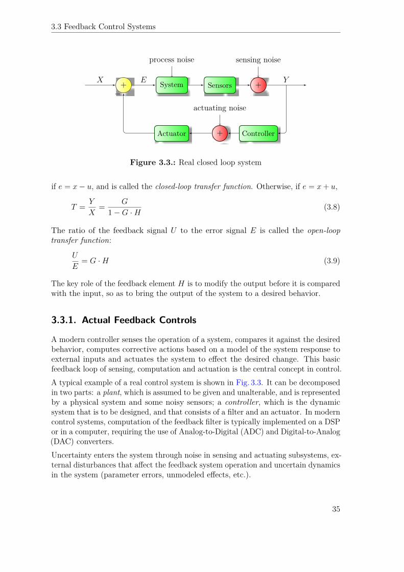
Figure 3.3.: Real closed loop system

if e = x− u, and is called the closed-loop transfer function. Otherwise, if e = x+ u,

T = Y

X= G

1−G ·H (3.8)

The ratio of the feedback signal U to the error signal E is called the open-looptransfer function:

U

E= G ·H (3.9)

The key role of the feedback element H is to modify the output before it is comparedwith the input, so as to bring the output of the system to a desired behavior.

3.3.1. Actual Feedback Controls

A modern controller senses the operation of a system, compares it against the desiredbehavior, computes corrective actions based on a model of the system response toexternal inputs and actuates the system to effect the desired change. This basicfeedback loop of sensing, computation and actuation is the central concept in control.A typical example of a real control system is shown in Fig. 3.3. It can be decomposedin two parts: a plant, which is assumed to be given and unalterable, and is representedby a physical system and some noisy sensors; a controller, which is the dynamicsystem that is to be designed, and that consists of a filter and an actuator. In moderncontrol systems, computation of the feedback filter is typically implemented on a DSPor in a computer, requiring the use of Analog-to-Digital (ADC) and Digital-to-Analog(DAC) converters.Uncertainty enters the system through noise in sensing and actuating subsystems, ex-ternal disturbances that affect the feedback system operation and uncertain dynamicsin the system (parameter errors, unmodeled effects, etc.).

35

Chapter 3 An Introduction to Control Theory

3.3.2. Advantages and Disadvantages

An advantage of the closed-loop control system is that the use of a well designedfeedback makes the system response relatively insensitive to external disturbancesand internal variations in system parameters that always occur. It is thus possible touse relatively inaccurate and inexpensive components to obtain the accurate controlof a given plant, whereas doing so is impossible in the open-loop case.On the other hand, stability is a major problem in the closed-loop control system,which may tend to over correct errors, thereby causing instability. An open-loopcontrol system is easier to build because system stability is not a major problem: aseries connection of two stable system is always stable. [22]Moreover, the actuation of a feedback control usually introduces unwanted noise tothe system. The signal-to-noise ratio cannot be improved using a feedback control.This can be proved analytically or just following a simple idea: a controller is notable to distinguish signal from noise. It amplifies and processes everything withoutdistinctions. It’s important to remember this: the purpose of a feedback control isnot the improvement of the Signal-to-Noise Ratio (SNR).

3.4. Stability of a Linear System

There are several ways to investigate the stability of a closed-loop system. Let’s takeinto account the denominator 1 +G ·H of the transfer function 3.7. The equation

1 +G ·H = 0 (3.10)

is called characteristic equation of the system. Its roots are called poles of the systemand their position in s plane strongly determines the stability of the system. It’spossible to demonstrate that a system is stable if and only if all of them lie in theleft-half s plane.

3.4.1. Nyquist Stability Criterion

The Nyquist stability criterion is a powerful tool to analyze the stability of a systemusing its open-loop transfer function. It states that

the closed-loop system is stable if and only if the graph in the s planeof the open-loop transfer function G (iω) · H (iω) for −∞ < ω < +∞,encircles the point −1 as many times anticlockwise as G (s) ·H (s) hasright half-plane poles (provided that there are no hidden unstable modescaused by unwanted cancellations of poles and zeros in the closed-loopsystem). [23]

36

4Digital Filters

Despite the work of this thesis consists in the implementation of a digital filter,the techniques so far described are to be applied to analog systems. Luckily it isquite simple to extend these concepts to the digital world, also because often digitalsignals are derived from analog signals by periodic sampling. Almost everything incontinuous-time systems has a counterpart in discrete-time systems.In this chapter are presented definitions and basic techniques to handle a digitalsystem, that will be used later in this thesis.

4.1. Definitions

Before continuing, it is useful to make some definitions. It’s possible to distinguishtwo families of signals:• continuous-time signals, defined at any value of the time variable t, and thus

represented by continuous variable functions;• discrete-time signals, defined only at discrete times and so represented as

sequences of number.Furthermore, also the amplitude of the signals can be either continuous or discrete.So, signals are also grouped in:• analog signals, when both time and amplitude are continuous;• digital signals, when both time and amplitude are discrete.

Similarly, continuous-time systems are systems for which both the input and outputare continuous-time signals and discrete-time systems are those for which the inputand output are discrete-time signals; analog systems are systems for which the inputand output are analog signals and digital systems are those for which both input andoutput are digital signals.

37

Chapter 4 Digital Filters

4.2. Linear Shift-Invariant Systems

As we have already seen, it is very useful to study a system in the frequency domainusing Laplace transform: the first thing to do is to extend it to discrete-time signals.For discrete-time systems, the natural replacement is the Z-transform Z [·], definedin Appendix A together with some properties.An important class of discrete-time systems is represented by the Linear Shift-Invariant systems for which the input x (n) and the output y (n) satisfy an N th-orderlinear constant-coefficient difference equation of the form

N∑k=0

aky (n− k) =M∑r=0brx (n− r) (4.1)

Shift-invariant means that if y (n) is the response to x (n), then y (n− k) is theresponse to x (n− k), ∀k ∈ Z. This class of system is the analogous, in the digitaldomain, of LTI systems described by equation 3.1.Similarly to 3.2, the transfer function of a linear shift-invariant system is defined asthe ratio of the Z-transform of the output to the Z-transform of the input:

G (z) = Y (z)X (z) =

M∑i=0biz−i

N∑j=0ajz−j

where we have used the Z-transform time shifting property Z [y (n− k)] = z−kZ [y (n)].As for Laplace transform, G represents also the Z-transform of the response to theunit-sample sequence

δ (n) =1 if n = 0

0 if n 6= 0(4.2)

whose Z-transform is Z [δ (n)] = 1.

4.3. Design of Digital Filters from Analog Filters

The traditional approach to the design of digital filters involves the transformationof an analog filter into a digital filter, meeting prescribed specifications. This is areasonable approach because:

1. the art of analog filter design is highly advanced and it is favorable to utilizethe design procedures already developed for analog filters, that usually arerather simple to implement;

38

4.3 Design of Digital Filters from Analog Filters

2. in many applications it is interesting to use a digital filter to simulate theperformance of an LTI analog filter.

Transforming an analog system to a digital system is tantamount to obtain a discrete-time transfer function Gd (z) from a continuous-time transfer function Ga (s). Insuch transformation we generally require that the essential properties of the analogfrequency response be preserved in the frequency response of the resulting digitalfilter. Loosely speaking, this implies that we want the imaginary axis of the s-planeto map into the unit circle of the z-plane. A second condition is that a stable analogfilter should be transformed to a stable digital filter. That is, if the analog systemhas poles only in the left-half s-plane, then the digital filter must have poles onlyinside the unit circle. [24] A common procedure that satisfies these requirements iscalled bilinear transformation and it is described in sec. A.3. It states that is possibleto obtain Gd (z) from Ga (s) with these two conditions by the substitution

s→ 2T

1− z−1

1 + z−1 (4.3)

where T is the sampling period. It’s easy to prove that the s-plane imaginary axis ismapped in the z-plane unit circle. Indeed, according to equation 4.3, points in theunit circle, where

z = eiωdT (4.4)

are mapped in purely imaginary s = iωa:

s = 2T

1− e−iωdT

1 + e−iωdT= i

2T

tan(T

2 ωd)

= iωa

That is, the discrete-time filter behaves at frequency ω the same way that thecontinuous-time filter behaves at frequency ωa

ωa = 2T

tan(T

2 ωd)

(4.5)

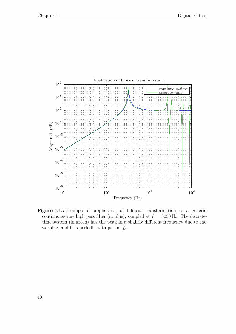
This means that every feature that is visible in the frequency response of thecontinuous-time filter is also visible in the discrete-time filter, but at a different fre-quency, as shown in the example in Fig. 4.1. This effect of the bilinear transformationis called frequency warping, and it can be neglected for frequencies ωd 2/T , whereωd ≈ ωa. However some applications inside Virgo require a so high precision thatthis effect must be considered: for example there are some high-Q notch filters whosecut-frequencies must to be placed with very high precision. This is done by pre-warping the filter design, that is designing the continuous-time filter to compensatefor this effect.The periodicity of equation 4.5 is a direct consequence of the aliasing predicted byNyquist sampling theorem.

39

Chapter 4 Digital Filters

10−1

100

101

102

10−6

10−5

10−4

10−3

10−2

10−1

100

101

102

Frequency (Hz)

Magnitude(dB)

Application of bilinear transformation

continuous-timediscrete-time

Figure 4.1.: Example of application of bilinear transformation to a genericcontinuous-time high pass filter (in blue), sampled at fc = 3030Hz. The discrete-time system (in green) has the peak in a slightly different frequency due to thewarping, and it is periodic with period fc.

40

5Seismic Isolation System in Advanced Virgo

This chapter describes the operation of the seismic isolation system in AdvancedVirgo, explaining how (and how much) they are able to attenuate the seismic noiseat the level of the optical elements of the interferometer.

5.1. Seismic Noise

The sensitivity of interferometric antennas for gravitational waves is limited at lowfrequency by seismic noise. This term indicates the stochastic movements of the soil,due to a multitude of causes that include nearby anthropogenic activities (such astraffic or heavy machinery), as well as natural phenomena like wind, sea waves, theposition of the moon, ...

Its Power Spectral Density (PSD) at ground level is not flat, and strongly dependson environmental conditions. An empiric estimation (also known as standard seismicnoise) is

Sx0 (f) ∼∣∣∣∣∣∣10−7

(1Hzf

)2 m√Hz

∣∣∣∣∣∣2

(5.1)

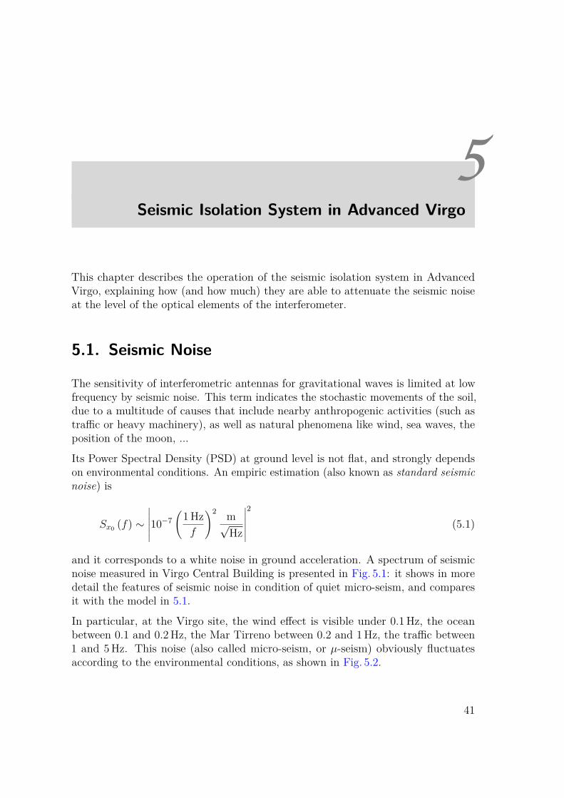
and it corresponds to a white noise in ground acceleration. A spectrum of seismicnoise measured in Virgo Central Building is presented in Fig. 5.1: it shows in moredetail the features of seismic noise in condition of quiet micro-seism, and comparesit with the model in 5.1.

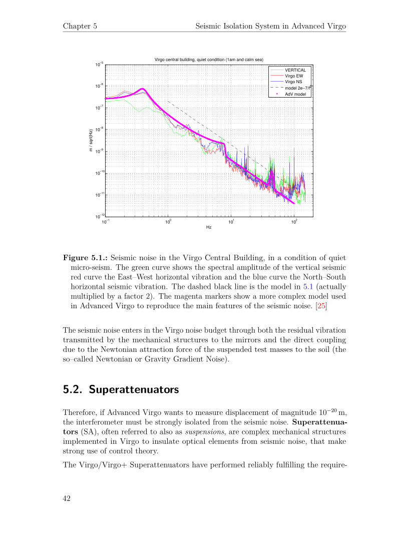
In particular, at the Virgo site, the wind effect is visible under 0.1Hz, the oceanbetween 0.1 and 0.2Hz, the Mar Tirreno between 0.2 and 1Hz, the traffic between1 and 5Hz. This noise (also called micro-seism, or µ-seism) obviously fluctuatesaccording to the environmental conditions, as shown in Fig. 5.2.

41

Chapter 5 Seismic Isolation System in Advanced Virgo

10−1 100 101 10210−12

10−11

10−10

10−9

10−8

10−7

10−6

10−5

Hz

m /

sqrt(

Hz)

Virgo central building, quiet condition (1am and calm sea)

VERTICALVirgo EWVirgo NSmodel 2e−7/f2

AdV model

Figure 5.1.: Seismic noise in the Virgo Central Building, in a condition of quietmicro-seism. The green curve shows the spectral amplitude of the vertical seismicred curve the East–West horizontal vibration and the blue curve the North–Southhorizontal seismic vibration. The dashed black line is the model in 5.1 (actuallymultiplied by a factor 2). The magenta markers show a more complex model usedin Advanced Virgo to reproduce the main features of the seismic noise. [25]

The seismic noise enters in the Virgo noise budget through both the residual vibrationtransmitted by the mechanical structures to the mirrors and the direct couplingdue to the Newtonian attraction force of the suspended test masses to the soil (theso–called Newtonian or Gravity Gradient Noise).

5.2. Superattenuators

Therefore, if Advanced Virgo wants to measure displacement of magnitude 10−20 m,the interferometer must be strongly isolated from the seismic noise. Superattenua-tors (SA), often referred to also as suspensions, are complex mechanical structuresimplemented in Virgo to insulate optical elements from seismic noise, that makestrong use of control theory.The Virgo/Virgo+ Superattenuators have performed reliably fulfilling the require-

42

5.2 Superattenuators

Figure 5.2.: Statistical property of the spectral amplitude of the micro-seismicdisplacement noise measured in the Virgo Central Building. For each frequencybin, it is reconstructed the probability to find a seismic amplitude below thethreshold indicated by each curve. [25]

ments and, since the time of project design, their passive attenuation performancewas considered to be compliant with the AdV requirements. Nevertheless, even ifthe essence of the suspension will be kept unchanged, some upgrades of mechanicaland electronic elements are ongoing, in order to achieve better performances duringperiods with adverse meteorological conditions.

Advanced Virgo comprises 10 SAs all operating in Ultra-High Vacuum chambers.Seven SAs are installed in the central building while the additional three are locatedin north end, west end buildings (3 km far from central area) and mode cleanerbuilding. Two classes of SAs are at present foreseen, short and long, depending onactual chain length and number of seismic filters used in the chain.

They have been designed to fulfill two main specifications:

1. reduce ground vibration transmission, in order to make mirror residual dis-placement below the interferometer sensitivity starting from a few hertz andthus to make seismic noise negligible above 10Hz;

2. reduce the mirror swing displacement in the low frequency range below a fewhertz, where the seismic noise is amplified by the filter chain resonances.

We are going to see how these aims are fulfilled.

43

Chapter 5 Seismic Isolation System in Advanced Virgo

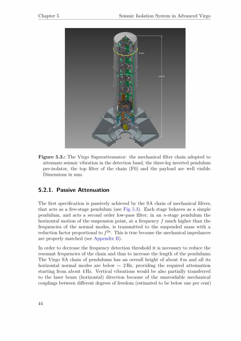
Figure 5.3.: The Virgo Superattenuator: the mechanical filter chain adopted toattenuate seismic vibration in the detection band, the three-leg inverted pendulumpre-isolator, the top filter of the chain (F0) and the payload are well visible.Dimensions in mm.

5.2.1. Passive Attenuation

The first specification is passively achieved by the SA chain of mechanical filters,that acts as a five-stage pendulum (see Fig. 5.3). Each stage behaves as a simplependulum, and acts a second order low-pass filter; in an n-stage pendulum thehorizontal motion of the suspension point, at a frequency f much higher than thefrequencies of the normal modes, is transmitted to the suspended mass with areduction factor proportional to f 2n. This is true because the mechanical impedancesare properly matched (see Appendix B).

In order to decrease the frequency detection threshold it is necessary to reduce theresonant frequencies of the chain and thus to increase the length of the pendulums.The Virgo SA chain of pendulums has an overall height of about 8m and all itshorizontal normal modes are below ∼ 2Hz, providing the required attenuationstarting from about 4Hz. Vertical vibrations would be also partially transferredto the laser beam (horizontal) direction because of the unavoidable mechanicalcouplings between different degrees of freedom (estimated to be below one per cent)

44

5.2 Superattenuators

and because of the Earth curvature that makes widely separated pendulums nonparallel to each other (misalignment of 3× 10−4 rad for 3 km-long arms).The top stage of the chain is formed by another mechanical filter named Filter 0 (F0)lying over a top table suspended by thin wires from a pre-isolation tripod, usuallycalled Inverted Pendulum (IP): in AdV its three legs are monolithic, made by asingle aluminum tube, in order to avoid dangerous yielding in the junctions andto eliminate undesired structural modes due to the presence of intermediate links.IP modes will be at 30− 40mHz, achieving a significant seismic attenuation in thehorizontal direction also in the pendulum chain resonance range (0.1− 2Hz).The 4 middle stages are called Standard Filters (SF). A SF is essentially a rigid steelcylinder (70 cm in diameter and 18.5 cm in height) supporting a set of maraging steelcantilevered triangular blades clamped along the outer surface of the filter body.Once properly loaded, the main vertical resonance of the blade system is around1.5Hz, that becomes < 0.5Hz under the effects of the anti-springs, devices installedon SF to reduce the frequencies of the vertical resonances. [26]SFs precede the last stage called, for historical reason, Filter 7 (F7). It was designedto suspend and steer the payload, a system that is composed by the marionette andthe mirror. The marionette allows the steering of the mirror with electromagneticactuators in three degrees of freedom. In Virgo/Virgo+, F7 included the referencemass, that was designed to compensate the recoil of the mirror. However, it isremoved in the new AdV payload design.

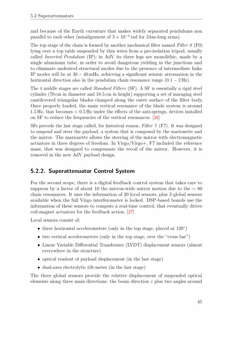
5.2.2. Superattenuator Control System

For the second scope, there is a digital feedback control system that takes care tosuppress by a factor of about 10 the micron-wide mirror motion due to the ∼ 80chain resonances. It uses the information of 20 local sensors, plus 3 global sensorsavailable when the full Virgo interferometer is locked. DSP-based boards use theinformation of these sensors to compute a real-time control, that eventually drivescoil-magnet actuators for the feedback action. [27]Local sensors consist of:• three horizontal accelerometers (only in the top stage, placed at 120)• two vertical accelerometers (only in the top stage, over the “cross bar”)• Linear Variable Differential Transformer (LVDT) displacement sensors (almost

everywhere in the structure)• optical readout of payload displacement (in the last stage)• dual-axes electrolytic tilt-meter (in the last stage)

The three global sensors provide the relative displacement of suspended opticalelements along three main directions: the beam direction z plus two angles around

45

Chapter 5 Seismic Isolation System in Advanced Virgo

Figure 5.4.: Top stage of the North Input Superattenuator. One of the threehorizontal accelerometer is highlighted in the red circle.

second horizontal axis x and vertical axis y. They are defined as global becausethe information is provided by the Virgo global control through the status of thewhole interferometer, and not of a single Superattenuator. Coil-magnet actuators areplaced at the top stage and at the F7 level, on the marionette and directly on themirror (except for the piezo actuators that are going to be placed at the base of IP).

The feedback control software is called Inertial Damping (ID). It runs on dedicatedboards, exploiting the huge computing power of modern DSPs. Two distinct DSPscontrol independently the top stage and the payload.

In particular, top stage control loops are always active regardless of the status of theinterferometer (i.e. not only when the interferometer is locked acquiring data). Itssensors monitor the displacement of the top stage in the DC − 100Hz bandwidthwith an equivalent sensitivity of 10−11 m√

Hz for accelerometers, and 10−8 m√Hz for LVDT

displacement sensors. The digital control loop operates at 10 kHz sampling frequency,the minimum rate required in order to avoid the introduction of actuation noise inthe gravitational wave detection bandwidth. Three degrees of freedom are currently

46

5.3 Control System towards Advanced Virgo

controlled (two translations in the horizontal plane and the rotation along the verticalaxis), and a forth one (vertical translation) is active in some suspensions. The lastVirgo+ performances allowed a residual displacement less than 1 µm at the level ofsuspended payload and a relative speed between long arm cavities input and endmirrors of about 0.25 µm/s, compliant with AdV requirements.Payload control system works a little bit differently, allowing two different opera-tional modes: when the interferometer is unlocked, payload control makes use ofmeasurements made in respect with a local reference frame, while, when the Virgointerferometer is in locked state, payload control uses the set points distributedby global control and alignment computers. Also here there are three controllabledegrees of freedom: longitudinal displacement (along the Virgo laser beam direction,z), rotation around the vertical axis and rotation along the horizontal axis orthogonalto laser beam direction. Only small corrections can be achieved in this stage, sothat the low frequency part of the z error signal is forwarded to top stage control,where bigger displacement can be achieved. The performances of the payload controlsystem meet AdV requirements, allowing a residual angular displacement of lessthan 1 µrad using local sensors and less than 1 nrad using global sensors, when theinterferometer is locked.In this way, SAs reduce the seismic noise by a factor 1015 at 10Hz, at the levelof the mirrors (see Fig. 5.5 for the complete transfer function). During Virgo dataacquisition runs, the control system did not limit neither sensitivity nor duty cycle,that was close to 100%. [2]

5.3. Control System towards Advanced Virgo

As already described in the previous sections, several changes to the mechanicalstructure of Virgo SA are in progress to fulfill AdV requirements. Of course, theseare not the only improvements.

5.3.1. Gyroscope and Tilt Control

The introduction of gyroscopes has been taken into account, in order to monitor adegree of freedom poorly controlled in Virgo, that dominates the seismic noise at lowfrequency: the tilt. Indeed, even if ground seismic tilt was never directly measuredby our site, we expect, under “good weather” conditions, a power spectrum densityin the order of

Stilt (f) ∼∣∣∣∣∣10−7

(1Hzf

)rad√Hz

∣∣∣∣∣2

(5.2)

Of course this value strongly depends on the weather conditions, and can grow a lotin the low frequency region in presence of strong wind and remote earthquakes, just

47

Chapter 5 Seismic Isolation System in Advanced Virgo

like the “ordinary” seismic noise. [28] Accelerometers on SA top stage are sensitiveboth to tilt and acceleration, making impossible to decouple two independent degreesof freedom that cannot be controlled in the same way. Indeed, if a traditionalaccelerometer subject to a gravitational acceleration g is tilted an angle α withrespect the vertical direction, it detect an acceleration

a = g sinα

Problems occur when a tilt produces a signal that is misinterpreted as a horizontalacceleration by the control loop, and loop forces the top stage to move even inabsence of horizontal displacement of the ground. This is why a pure-tilt inertialsensor is mandatory to increase the duty-cycle of the interferometer, subtracting thetilt signal from the IP accelerometers and then providing the error for its control. [29]According to some estimations, a tilt control system implemented on the SA wouldbe the straightforward solution to reduce by at least one order of magnitude themirror swing in 0 − 200mHz range and to fulfill AdV specifications with a widesafety margin in any weather conditions.However, even if this problems is known since the construction of the first Virgo, asuitable sensor is difficult to source mostly due to the high sensitivity required, thatshall be at the level of 10−8 rad√

Hz in the tens of mHz band. Several kind of gyroscopeshas been analyzed since the beginning of Virgo project, but none of them has beenfound complying gravitational wave detector requirements.A prototype of a single axis Hemispherical Resonator Gyroscope (HRG) producedby Medicon (Russia) is currently under test by INFN Pisa Virgo group. HRG arethe de facto standard gyroscopes used in the inertial guidance of space missions(launched aboard more than 100 spacecrafts). A recent measurement performed byVirgo Pisa group discloses that this kind of gyroscope is so far the most suitablesensor for our purpose and, even if the knowledge of this devices is still too modestto hypothesize an implementation in AdV, they are probably going to became partof the experiment in the next future.In the meanwhile, an alternative approach is under investigation, that consist in theextrapolation of the tilt from accelerometers and LVDT displacement sensors. Thisbecause theoretically the position of a rigid body has six degrees of freedom, andcan be detected by six independent sensors.Regarding the actuators for the tilt control, piezoelectric actuators are going to beinstalled below the bottom flange supporting the three IP feet. It is also possible toconceive the use of these actuators to compensate the excess of vertical seismic noiseon the suspension top stage, presently exciting the angular payload motion.

5.3.2. Electronics

In order to ensure a long term operation and maintenance for AdV, and to overcomethe physical and technical obsolescence of hardware, the Superattenuator electronics

48

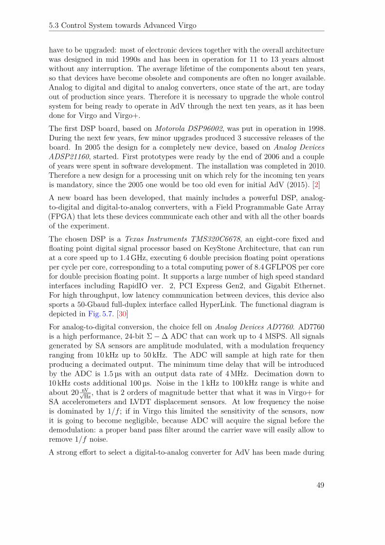
5.3 Control System towards Advanced Virgo

have to be upgraded: most of electronic devices together with the overall architecturewas designed in mid 1990s and has been in operation for 11 to 13 years almostwithout any interruption. The average lifetime of the components about ten years,so that devices have become obsolete and components are often no longer available.Analog to digital and digital to analog converters, once state of the art, are todayout of production since years. Therefore it is necessary to upgrade the whole controlsystem for being ready to operate in AdV through the next ten years, as it has beendone for Virgo and Virgo+.The first DSP board, based on Motorola DSP96002, was put in operation in 1998.During the next few years, few minor upgrades produced 3 successive releases of theboard. In 2005 the design for a completely new device, based on Analog DevicesADSP21160, started. First prototypes were ready by the end of 2006 and a coupleof years were spent in software development. The installation was completed in 2010.Therefore a new design for a processing unit on which rely for the incoming ten yearsis mandatory, since the 2005 one would be too old even for initial AdV (2015). [2]A new board has been developed, that mainly includes a powerful DSP, analog-to-digital and digital-to-analog converters, with a Field Programmable Gate Array(FPGA) that lets these devices communicate each other and with all the other boardsof the experiment.The chosen DSP is a Texas Instruments TMS320C6678, an eight-core fixed andfloating point digital signal processor based on KeyStone Architecture, that can runat a core speed up to 1.4GHz, executing 6 double precision floating point operationsper cycle per core, corresponding to a total computing power of 8.4GFLPOS per corefor double precision floating point. It supports a large number of high speed standardinterfaces including RapidIO ver. 2, PCI Express Gen2, and Gigabit Ethernet.For high throughput, low latency communication between devices, this device alsosports a 50-Gbaud full-duplex interface called HyperLink. The functional diagram isdepicted in Fig. 5.7. [30]For analog-to-digital conversion, the choice fell on Analog Devices AD7760. AD7760is a high performance, 24-bit Σ−∆ ADC that can work up to 4 MSPS. All signalsgenerated by SA sensors are amplitude modulated, with a modulation frequencyranging from 10 kHz up to 50 kHz. The ADC will sample at high rate for thenproducing a decimated output. The minimum time delay that will be introducedby the ADC is 1.5 µs with an output data rate of 4MHz. Decimation down to10 kHz costs additional 100 µs. Noise in the 1 kHz to 100 kHz range is white andabout 20 nV√

Hz , that is 2 orders of magnitude better that what it was in Virgo+ forSA accelerometers and LVDT displacement sensors. At low frequency the noiseis dominated by 1/f ; if in Virgo this limited the sensitivity of the sensors, nowit is going to become negligible, because ADC will acquire the signal before thedemodulation: a proper band pass filter around the carrier wave will easily allow toremove 1/f noise.A strong effort to select a digital-to-analog converter for AdV has been made during

49

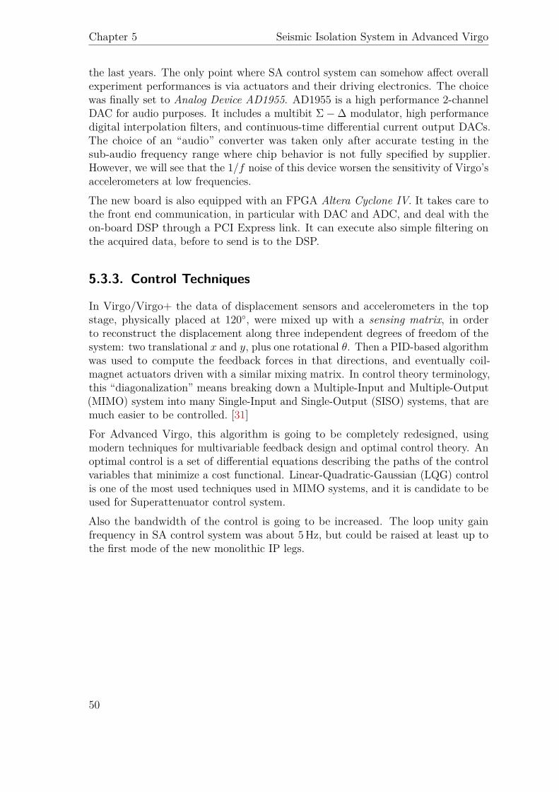
Chapter 5 Seismic Isolation System in Advanced Virgo

the last years. The only point where SA control system can somehow affect overallexperiment performances is via actuators and their driving electronics. The choicewas finally set to Analog Device AD1955. AD1955 is a high performance 2-channelDAC for audio purposes. It includes a multibit Σ−∆ modulator, high performancedigital interpolation filters, and continuous-time differential current output DACs.The choice of an “audio” converter was taken only after accurate testing in thesub-audio frequency range where chip behavior is not fully specified by supplier.However, we will see that the 1/f noise of this device worsen the sensitivity of Virgo’saccelerometers at low frequencies.The new board is also equipped with an FPGA Altera Cyclone IV. It takes care tothe front end communication, in particular with DAC and ADC, and deal with theon-board DSP through a PCI Express link. It can execute also simple filtering onthe acquired data, before to send is to the DSP.

5.3.3. Control Techniques

In Virgo/Virgo+ the data of displacement sensors and accelerometers in the topstage, physically placed at 120, were mixed up with a sensing matrix, in orderto reconstruct the displacement along three independent degrees of freedom of thesystem: two translational x and y, plus one rotational θ. Then a PID-based algorithmwas used to compute the feedback forces in that directions, and eventually coil-magnet actuators driven with a similar mixing matrix. In control theory terminology,this “diagonalization” means breaking down a Multiple-Input and Multiple-Output(MIMO) system into many Single-Input and Single-Output (SISO) systems, that aremuch easier to be controlled. [31]For Advanced Virgo, this algorithm is going to be completely redesigned, usingmodern techniques for multivariable feedback design and optimal control theory. Anoptimal control is a set of differential equations describing the paths of the controlvariables that minimize a cost functional. Linear-Quadratic-Gaussian (LQG) controlis one of the most used techniques used in MIMO systems, and it is candidate to beused for Superattenuator control system.Also the bandwidth of the control is going to be increased. The loop unity gainfrequency in SA control system was about 5Hz, but could be raised at least up tothe first mode of the new monolithic IP legs.

50

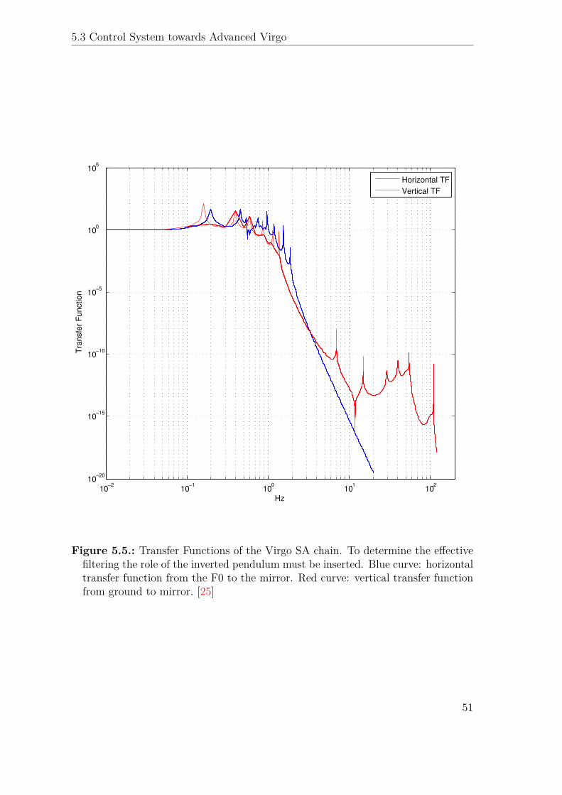
5.3 Control System towards Advanced Virgo

10−2 10−1 100 101 10210−20

10−15

10−10

10−5

100

105

Hz

Tra

nsfe

r Fun

ctio

n

Horizontal TFVertical TF

Figure 5.5.: Transfer Functions of the Virgo SA chain. To determine the effectivefiltering the role of the inverted pendulum must be inserted. Blue curve: horizontaltransfer function from the F0 to the mirror. Red curve: vertical transfer functionfrom ground to mirror. [25]

51

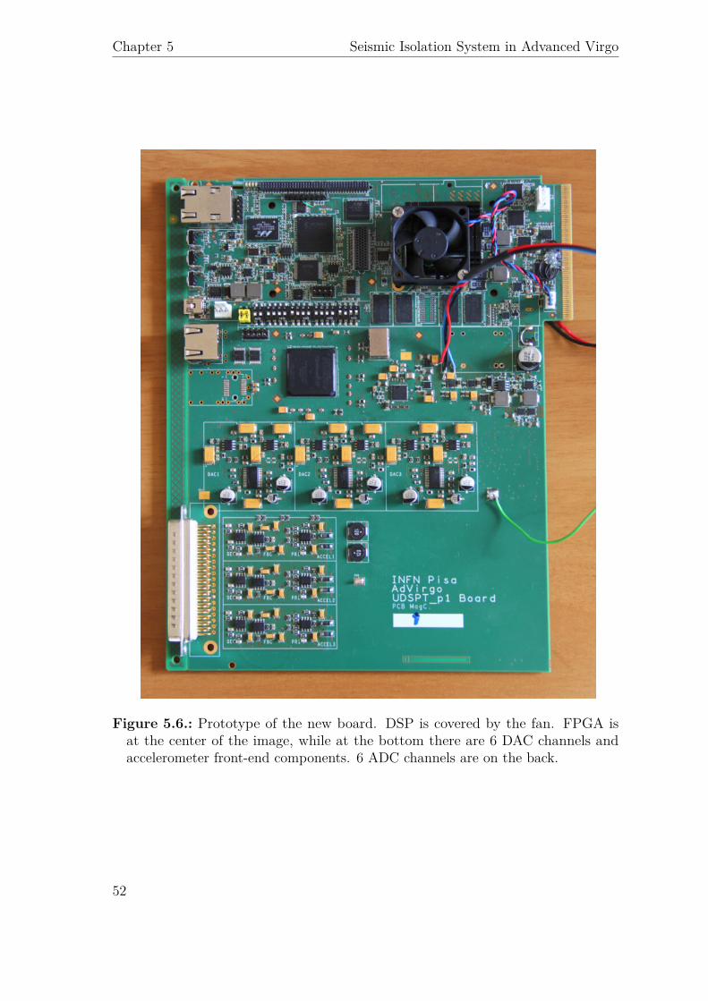
Chapter 5 Seismic Isolation System in Advanced Virgo

Figure 5.6.: Prototype of the new board. DSP is covered by the fan. FPGA isat the center of the image, while at the bottom there are 6 DAC channels andaccelerometer front-end components. 6 ADC channels are on the back.

52

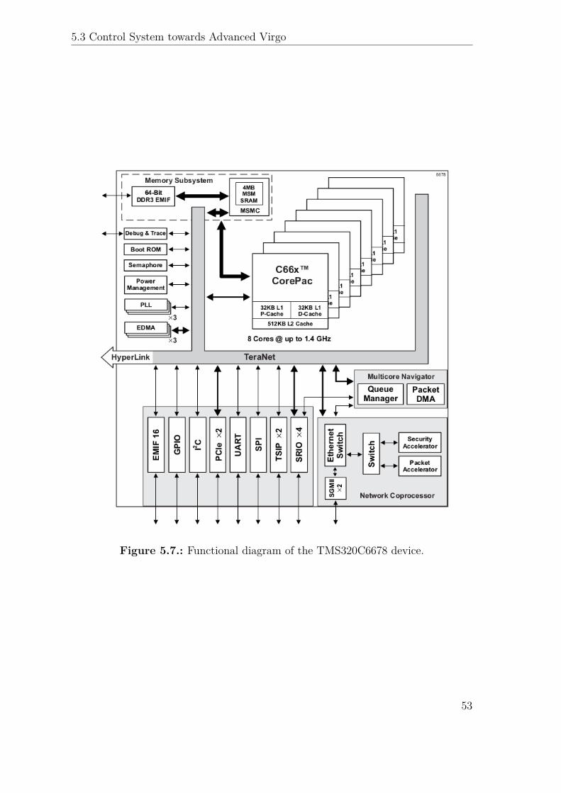
5.3 Control System towards Advanced Virgo

Figure 5.7.: Functional diagram of the TMS320C6678 device.

53

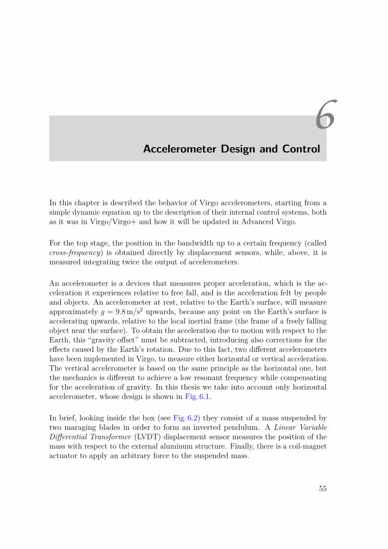
6Accelerometer Design and Control

In this chapter is described the behavior of Virgo accelerometers, starting from asimple dynamic equation up to the description of their internal control systems, bothas it was in Virgo/Virgo+ and how it will be updated in Advanced Virgo.

For the top stage, the position in the bandwidth up to a certain frequency (calledcross-frequency) is obtained directly by displacement sensors, while, above, it ismeasured integrating twice the output of accelerometers.

An accelerometer is a devices that measures proper acceleration, which is the ac-celeration it experiences relative to free fall, and is the acceleration felt by peopleand objects. An accelerometer at rest, relative to the Earth’s surface, will measureapproximately g = 9.8m/s2 upwards, because any point on the Earth’s surface isaccelerating upwards, relative to the local inertial frame (the frame of a freely fallingobject near the surface). To obtain the acceleration due to motion with respect to theEarth, this “gravity offset” must be subtracted, introducing also corrections for theeffects caused by the Earth’s rotation. Due to this fact, two different accelerometershave been implemented in Virgo, to measure either horizontal or vertical acceleration.The vertical accelerometer is based on the same principle as the horizontal one, butthe mechanics is different to achieve a low resonant frequency while compensatingfor the acceleration of gravity. In this thesis we take into account only horizontalaccelerometer, whose design is shown in Fig. 6.1.

In brief, looking inside the box (see Fig. 6.2) they consist of a mass suspended bytwo maraging blades in order to form an inverted pendulum. A Linear VariableDifferential Transformer (LVDT) displacement sensor measures the position of themass with respect to the external aluminum structure. Finally, there is a coil-magnetactuator to apply an arbitrary force to the suspended mass.

55

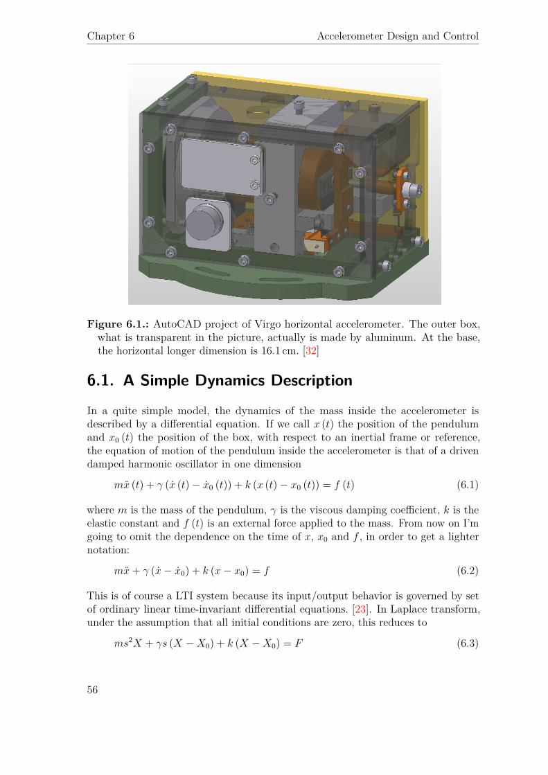
Chapter 6 Accelerometer Design and Control

Figure 6.1.: AutoCAD project of Virgo horizontal accelerometer. The outer box,what is transparent in the picture, actually is made by aluminum. At the base,the horizontal longer dimension is 16.1 cm. [32]

6.1. A Simple Dynamics Description

In a quite simple model, the dynamics of the mass inside the accelerometer isdescribed by a differential equation. If we call x (t) the position of the pendulumand x0 (t) the position of the box, with respect to an inertial frame or reference,the equation of motion of the pendulum inside the accelerometer is that of a drivendamped harmonic oscillator in one dimension

mx (t) + γ (x (t)− x0 (t)) + k (x (t)− x0 (t)) = f (t) (6.1)

where m is the mass of the pendulum, γ is the viscous damping coefficient, k is theelastic constant and f (t) is an external force applied to the mass. From now on I’mgoing to omit the dependence on the time of x, x0 and f , in order to get a lighternotation:

mx+ γ (x− x0) + k (x− x0) = f (6.2)

This is of course a LTI system because its input/output behavior is governed by setof ordinary linear time-invariant differential equations. [23]. In Laplace transform,under the assumption that all initial conditions are zero, this reduces to

ms2X + γs (X −X0) + k (X −X0) = F (6.3)

56

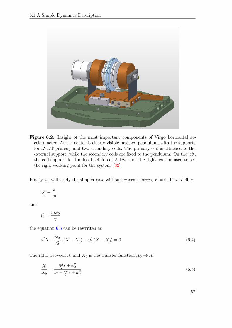
6.1 A Simple Dynamics Description

Figure 6.2.: Insight of the most important components of Virgo horizontal ac-celerometer. At the center is clearly visible inverted pendulum, with the supportsfor LVDT primary and two secondary coils. The primary coil is attached to theexternal support, while the secondary coils are fixed to the pendulum. On the left,the coil support for the feedback force. A lever, on the right, can be used to setthe right working point for the system. [32]

Firstly we will study the simpler case without external forces, F = 0. If we define

ω20 = k

m

and

Q = mω0

γ

the equation 6.3 can be rewritten as

s2X + ω0

Qs (X −X0) + ω2

0 (X −X0) = 0 (6.4)

The ratio between X and X0 is the transfer function X0 → X:

X

X0=

ω0Qs+ ω2

0

s2 + ω0Qs+ ω2

0(6.5)

57

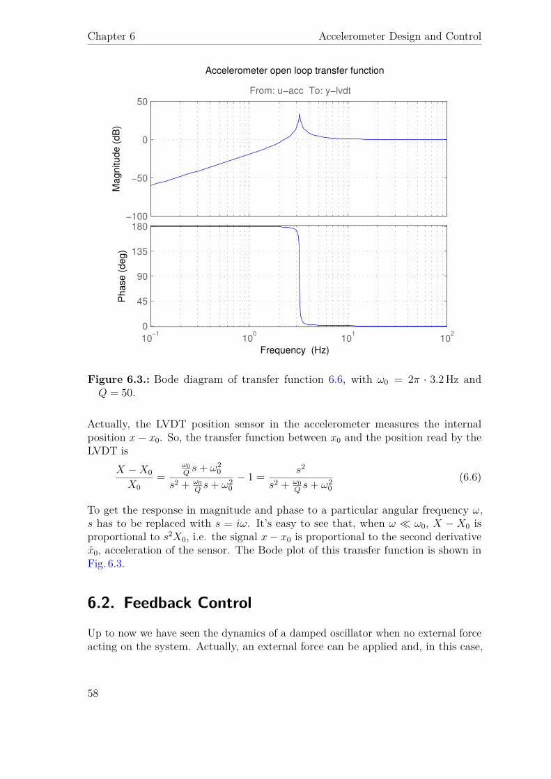
Chapter 6 Accelerometer Design and Control

−100

−50

0

50From: u−acc To: y−lvdt

Ma

gn

itu

de

(d

B)

10−1

100

101

102

0

45

90

135

180

Ph

ase

(d

eg

)

Accelerometer open loop transfer function

Frequency (Hz)

Figure 6.3.: Bode diagram of transfer function 6.6, with ω0 = 2π · 3.2Hz andQ = 50.

Actually, the LVDT position sensor in the accelerometer measures the internalposition x− x0. So, the transfer function between x0 and the position read by theLVDT is

X −X0

X0=

ω0Qs+ ω2

0

s2 + ω0Qs+ ω2

0− 1 = s2

s2 + ω0Qs+ ω2

0(6.6)

To get the response in magnitude and phase to a particular angular frequency ω,s has to be replaced with s = iω. It’s easy to see that, when ω ω0, X − X0 isproportional to s2X0, i.e. the signal x− x0 is proportional to the second derivativex0, acceleration of the sensor. The Bode plot of this transfer function is shown inFig. 6.3.

6.2. Feedback Control

Up to now we have seen the dynamics of a damped oscillator when no external forceacting on the system. Actually, an external force can be applied and, in this case,

58

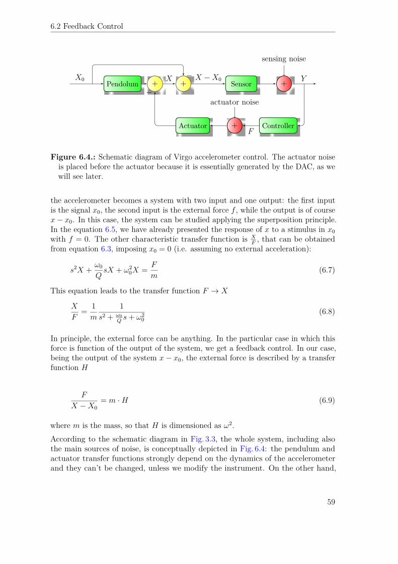
6.2 Feedback Control

Pendolum + + Sensor +

sensing noise

X0 X X −X0 Y

Controller+

actuator noise

Actuator

−

F

−

Figure 6.4.: Schematic diagram of Virgo accelerometer control. The actuator noiseis placed before the actuator because it is essentially generated by the DAC, as wewill see later.

the accelerometer becomes a system with two input and one output: the first inputis the signal x0, the second input is the external force f , while the output is of coursex− x0. In this case, the system can be studied applying the superposition principle.In the equation 6.5, we have already presented the response of x to a stimulus in x0with f = 0. The other characteristic transfer function is X

F, that can be obtained

from equation 6.3, imposing x0 = 0 (i.e. assuming no external acceleration):

s2X + ω0

QsX + ω2

0X = F

m(6.7)

This equation leads to the transfer function F → X

X

F= 1m

1s2 + ω0

Qs+ ω2

0(6.8)

In principle, the external force can be anything. In the particular case in which thisforce is function of the output of the system, we get a feedback control. In our case,being the output of the system x− x0, the external force is described by a transferfunction H

F

X −X0= m ·H (6.9)

where m is the mass, so that H is dimensioned as ω2.According to the schematic diagram in Fig. 3.3, the whole system, including alsothe main sources of noise, is conceptually depicted in Fig. 6.4: the pendulum andactuator transfer functions strongly depend on the dynamics of the accelerometerand they can’t be changed, unless we modify the instrument. On the other hand,

59

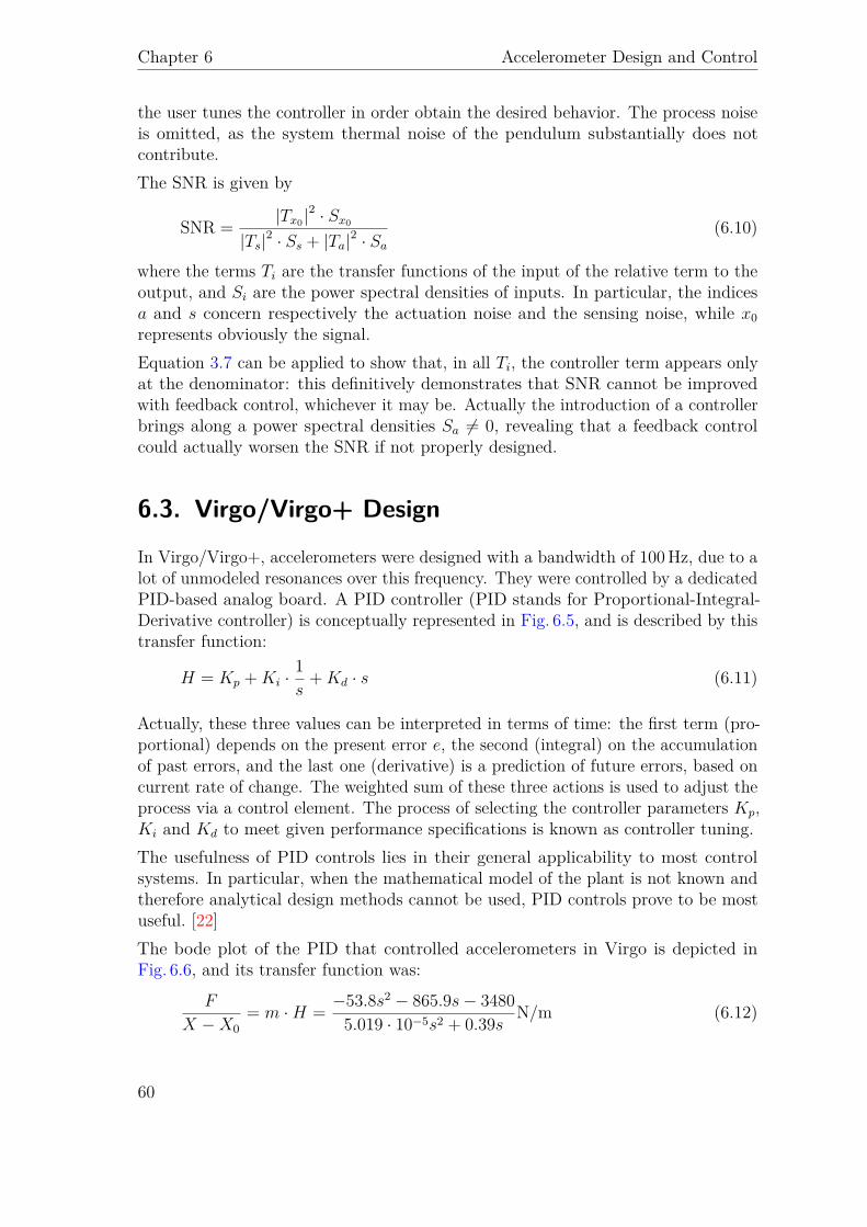
Chapter 6 Accelerometer Design and Control

the user tunes the controller in order obtain the desired behavior. The process noiseis omitted, as the system thermal noise of the pendulum substantially does notcontribute.The SNR is given by

SNR = |Tx0|2 · Sx0

|Ts|2 · Ss + |Ta|2 · Sa(6.10)

where the terms Ti are the transfer functions of the input of the relative term to theoutput, and Si are the power spectral densities of inputs. In particular, the indicesa and s concern respectively the actuation noise and the sensing noise, while x0represents obviously the signal.Equation 3.7 can be applied to show that, in all Ti, the controller term appears onlyat the denominator: this definitively demonstrates that SNR cannot be improvedwith feedback control, whichever it may be. Actually the introduction of a controllerbrings along a power spectral densities Sa 6= 0, revealing that a feedback controlcould actually worsen the SNR if not properly designed.

6.3. Virgo/Virgo+ Design

In Virgo/Virgo+, accelerometers were designed with a bandwidth of 100Hz, due to alot of unmodeled resonances over this frequency. They were controlled by a dedicatedPID-based analog board. A PID controller (PID stands for Proportional-Integral-Derivative controller) is conceptually represented in Fig. 6.5, and is described by thistransfer function:

H = Kp +Ki ·1s

+Kd · s (6.11)

Actually, these three values can be interpreted in terms of time: the first term (pro-portional) depends on the present error e, the second (integral) on the accumulationof past errors, and the last one (derivative) is a prediction of future errors, based oncurrent rate of change. The weighted sum of these three actions is used to adjust theprocess via a control element. The process of selecting the controller parameters Kp,Ki and Kd to meet given performance specifications is known as controller tuning.The usefulness of PID controls lies in their general applicability to most controlsystems. In particular, when the mathematical model of the plant is not known andtherefore analytical design methods cannot be used, PID controls prove to be mostuseful. [22]The bode plot of the PID that controlled accelerometers in Virgo is depicted inFig. 6.6, and its transfer function was:

F

X −X0= m ·H = −53.8s2 − 865.9s− 3480

5.019 · 10−5s2 + 0.39s N/m (6.12)

60

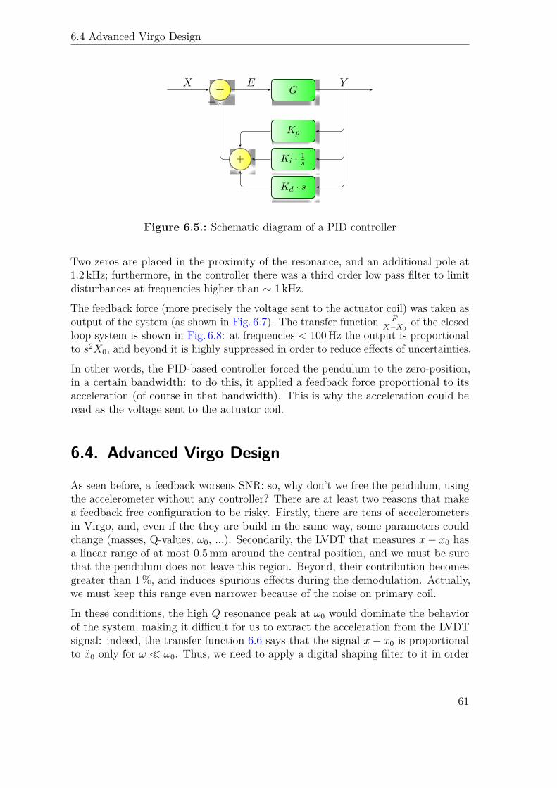
6.4 Advanced Virgo Design

+ G

Kp

Ki · 1s

Kd · s

+

X E Y

−

Figure 6.5.: Schematic diagram of a PID controller

Two zeros are placed in the proximity of the resonance, and an additional pole at1.2 kHz; furthermore, in the controller there was a third order low pass filter to limitdisturbances at frequencies higher than ∼ 1 kHz.

The feedback force (more precisely the voltage sent to the actuator coil) was taken asoutput of the system (as shown in Fig. 6.7). The transfer function F

X−X0of the closed

loop system is shown in Fig. 6.8: at frequencies < 100Hz the output is proportionalto s2X0, and beyond it is highly suppressed in order to reduce effects of uncertainties.

In other words, the PID-based controller forced the pendulum to the zero-position,in a certain bandwidth: to do this, it applied a feedback force proportional to itsacceleration (of course in that bandwidth). This is why the acceleration could beread as the voltage sent to the actuator coil.

6.4. Advanced Virgo Design

As seen before, a feedback worsens SNR: so, why don’t we free the pendulum, usingthe accelerometer without any controller? There are at least two reasons that makea feedback free configuration to be risky. Firstly, there are tens of accelerometersin Virgo, and, even if the they are build in the same way, some parameters couldchange (masses, Q-values, ω0, ...). Secondarily, the LVDT that measures x− x0 hasa linear range of at most 0.5mm around the central position, and we must be surethat the pendulum does not leave this region. Beyond, their contribution becomesgreater than 1%, and induces spurious effects during the demodulation. Actually,we must keep this range even narrower because of the noise on primary coil.

In these conditions, the high Q resonance peak at ω0 would dominate the behaviorof the system, making it difficult for us to extract the acceleration from the LVDTsignal: indeed, the transfer function 6.6 says that the signal x− x0 is proportionalto x0 only for ω ω0. Thus, we need to apply a digital shaping filter to it in order

61

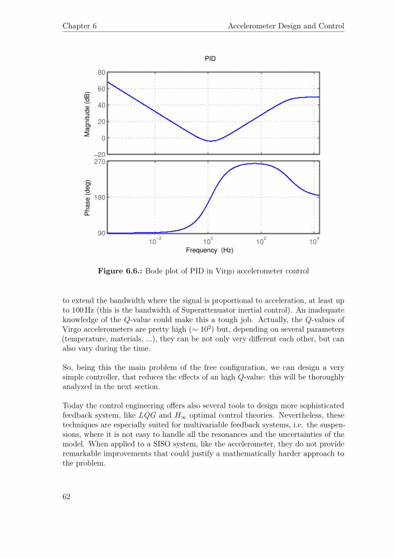
Chapter 6 Accelerometer Design and Control

−20

0

20

40

60

80

Magnitude (

dB

)

10−2

100

102

104

90

180

270

Phase (

deg)

PID

Frequency (Hz)

Figure 6.6.: Bode plot of PID in Virgo accelerometer control

to extend the bandwidth where the signal is proportional to acceleration, at least upto 100Hz (this is the bandwidth of Superattenuator inertial control). An inadequateknowledge of the Q-value could make this a tough job. Actually, the Q-values ofVirgo accelerometers are pretty high (∼ 102) but, depending on several parameters(temperature, materials, ...), they can be not only very different each other, but canalso vary during the time.

So, being this the main problem of the free configuration, we can design a verysimple controller, that reduces the effects of an high Q-value: this will be thoroughlyanalyzed in the next section.

Today the control engineering offers also several tools to design more sophisticatedfeedback system, like LQG and H∞ optimal control theories. Nevertheless, thesetechniques are especially suited for multivariable feedback systems, i.e. the suspen-sions, where it is not easy to handle all the resonances and the uncertainties of themodel. When applied to a SISO system, like the accelerometer, they do not provideremarkable improvements that could justify a mathematically harder approach tothe problem.

62

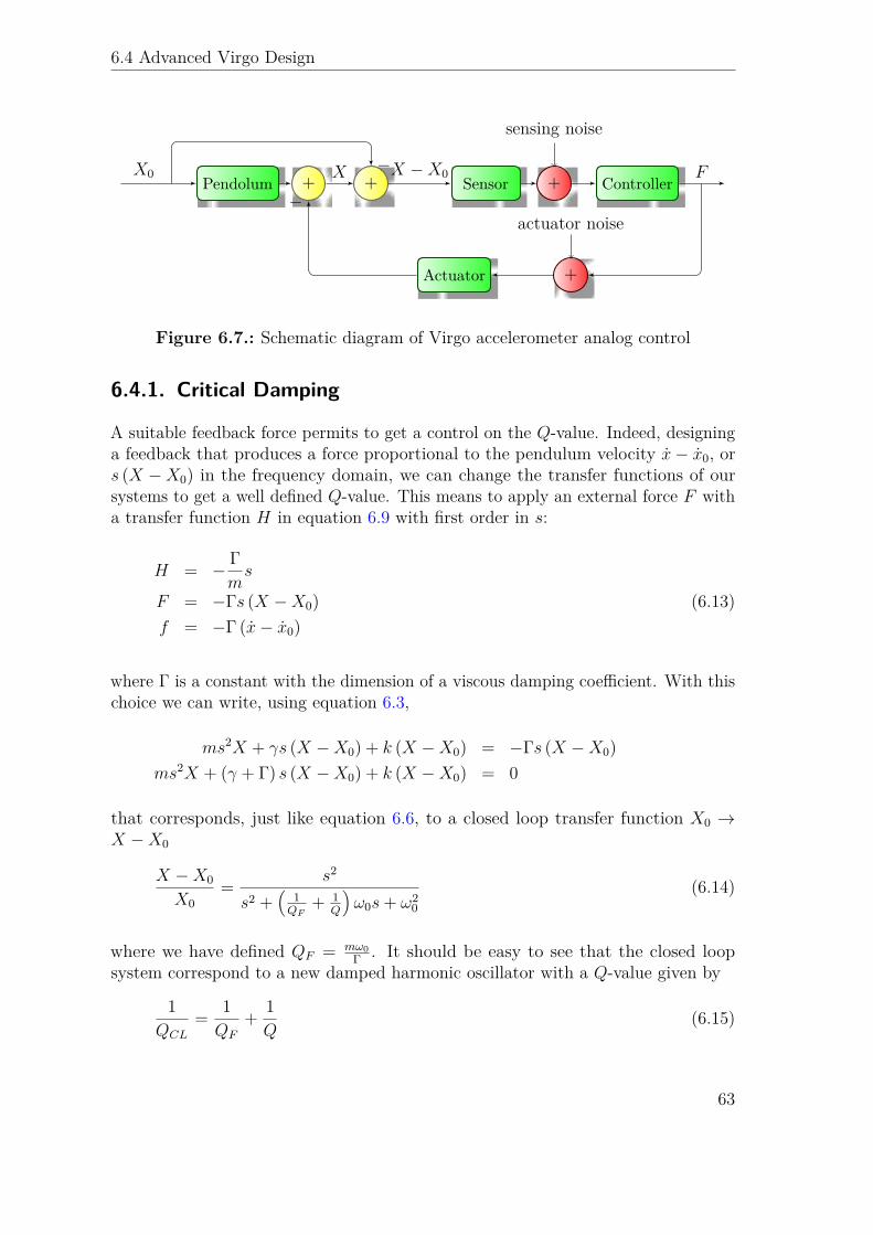
6.4 Advanced Virgo Design

Pendolum + + Sensor +

sensing noise

ControllerX0 X X −X0 F

+

actuator noise

Actuator

−

−

Figure 6.7.: Schematic diagram of Virgo accelerometer analog control

6.4.1. Critical Damping

A suitable feedback force permits to get a control on the Q-value. Indeed, designinga feedback that produces a force proportional to the pendulum velocity x− x0, ors (X −X0) in the frequency domain, we can change the transfer functions of oursystems to get a well defined Q-value. This means to apply an external force F witha transfer function H in equation 6.9 with first order in s:

H = − Γms

F = −Γs (X −X0) (6.13)f = −Γ (x− x0)

where Γ is a constant with the dimension of a viscous damping coefficient. With thischoice we can write, using equation 6.3,

ms2X + γs (X −X0) + k (X −X0) = −Γs (X −X0)ms2X + (γ + Γ) s (X −X0) + k (X −X0) = 0

that corresponds, just like equation 6.6, to a closed loop transfer function X0 →X −X0

X −X0

X0= s2

s2 +(

1QF

+ 1Q

)ω0s+ ω2

0(6.14)

where we have defined QF = mω0Γ . It should be easy to see that the closed loop

system correspond to a new damped harmonic oscillator with a Q-value given by

1QCL

= 1QF

+ 1Q

(6.15)

63

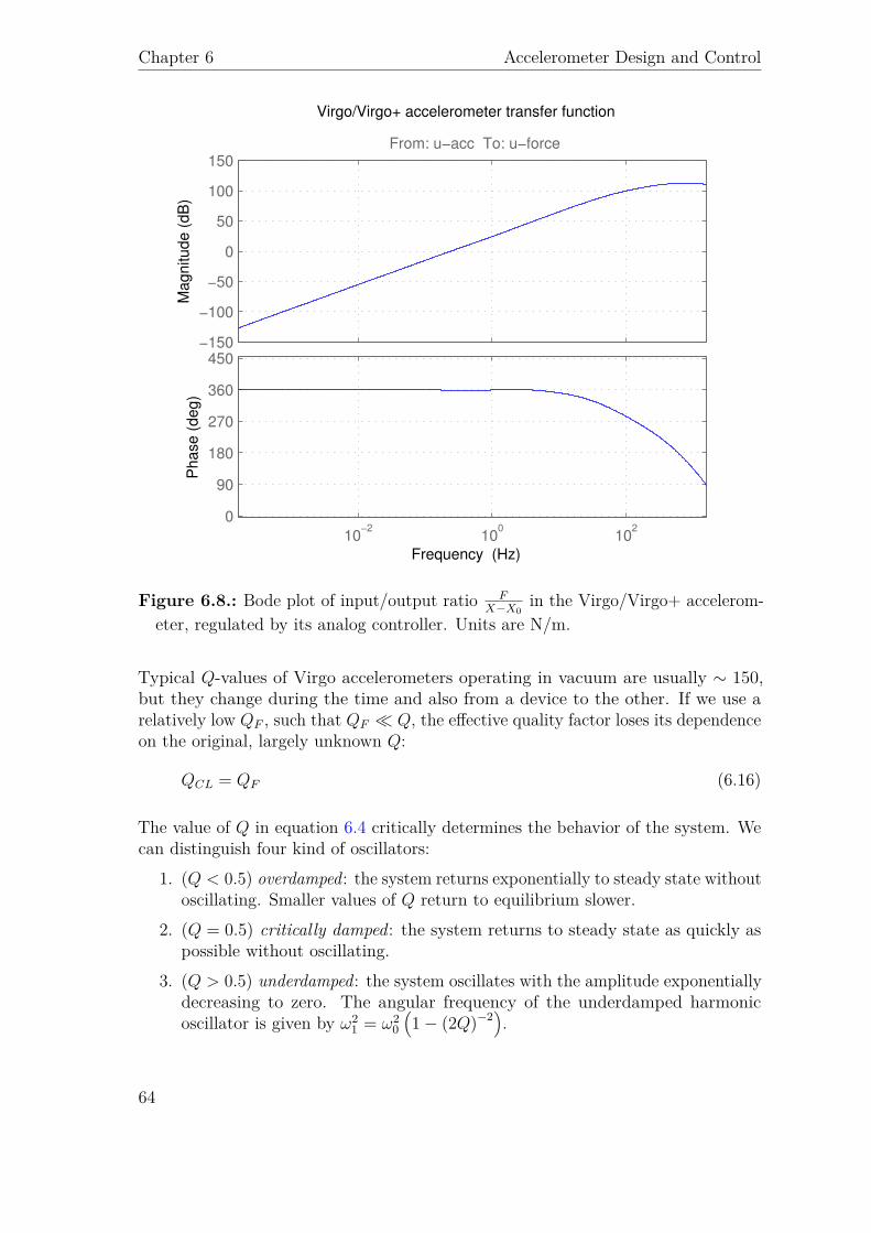
Chapter 6 Accelerometer Design and Control

−150

−100

−50

0

50

100

150From: u−acc To: u−force

Ma

gn

itu

de

(d

B)

10−2

100

102

0

90

180

270

360

450

Ph

ase

(d

eg

)

Virgo/Virgo+ accelerometer transfer function

Frequency (Hz)

Figure 6.8.: Bode plot of input/output ratio FX−X0

in the Virgo/Virgo+ accelerom-eter, regulated by its analog controller. Units are N/m.

Typical Q-values of Virgo accelerometers operating in vacuum are usually ∼ 150,but they change during the time and also from a device to the other. If we use arelatively low QF , such that QF Q, the effective quality factor loses its dependenceon the original, largely unknown Q:

QCL = QF (6.16)

The value of Q in equation 6.4 critically determines the behavior of the system. Wecan distinguish four kind of oscillators:

1. (Q < 0.5) overdamped: the system returns exponentially to steady state withoutoscillating. Smaller values of Q return to equilibrium slower.

2. (Q = 0.5) critically damped: the system returns to steady state as quickly aspossible without oscillating.

3. (Q > 0.5) underdamped: the system oscillates with the amplitude exponentiallydecreasing to zero. The angular frequency of the underdamped harmonicoscillator is given by ω2

1 = ω20

(1− (2Q)−2

).

64

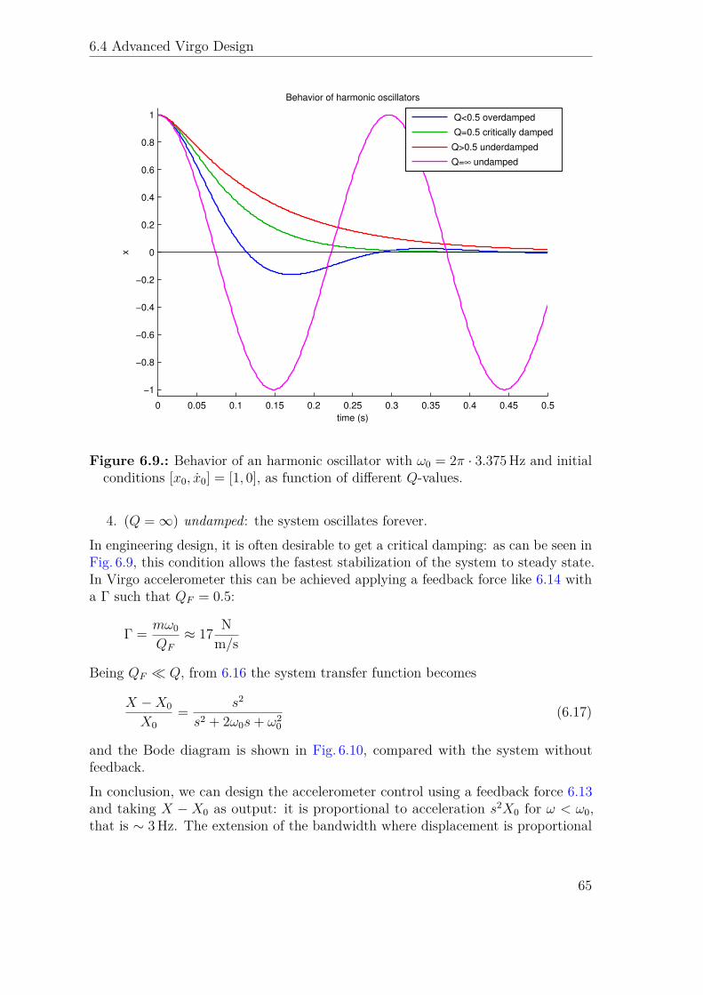
6.4 Advanced Virgo Design

0 0.05 0.1 0.15 0.2 0.25 0.3 0.35 0.4 0.45 0.5

−1

−0.8

−0.6

−0.4

−0.2

0

0.2

0.4

0.6

0.8

1

time (s)

x

Behavior of harmonic oscillators

Q<0.5 overdamped

Q=0.5 critically damped

Q>0.5 underdamped

Q=∞ undamped

Figure 6.9.: Behavior of an harmonic oscillator with ω0 = 2π · 3.375Hz and initialconditions [x0, x0] = [1, 0], as function of different Q-values.

4. (Q =∞) undamped: the system oscillates forever.In engineering design, it is often desirable to get a critical damping: as can be seen inFig. 6.9, this condition allows the fastest stabilization of the system to steady state.In Virgo accelerometer this can be achieved applying a feedback force like 6.14 witha Γ such that QF = 0.5:

Γ = mω0

QF

≈ 17 Nm/s

Being QF Q, from 6.16 the system transfer function becomes

X −X0

X0= s2

s2 + 2ω0s+ ω20

(6.17)

and the Bode diagram is shown in Fig. 6.10, compared with the system withoutfeedback.In conclusion, we can design the accelerometer control using a feedback force 6.13and taking X − X0 as output: it is proportional to acceleration s2X0 for ω < ω0,that is ∼ 3Hz. The extension of the bandwidth where displacement is proportional

65

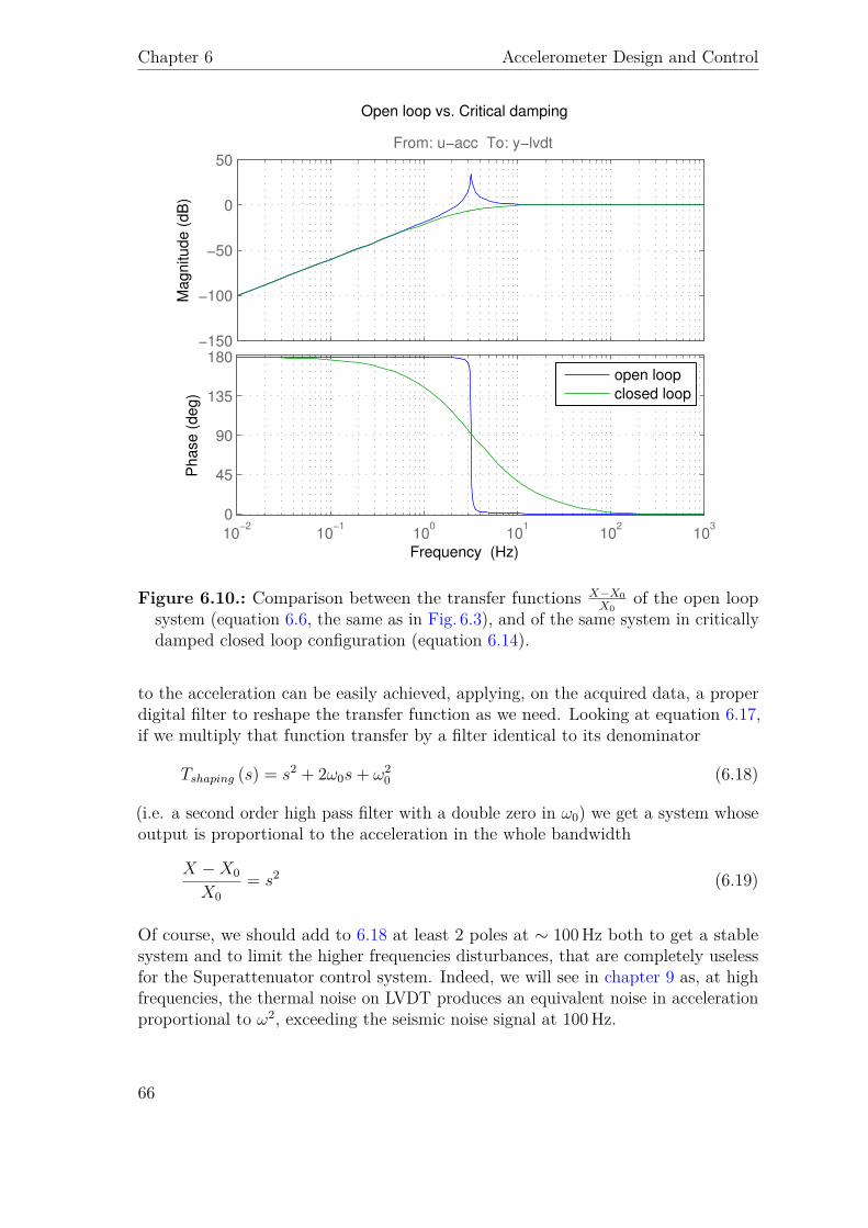
Chapter 6 Accelerometer Design and Control

−150

−100

−50

0

50From: u−acc To: y−lvdt

Ma

gn

itu

de

(d

B)

10−2

10−1

100

101

102

103

0

45

90

135

180

Ph

ase

(d

eg

)

Open loop vs. Critical damping

Frequency (Hz)

open loop

closed loop

Figure 6.10.: Comparison between the transfer functions X−X0X0

of the open loopsystem (equation 6.6, the same as in Fig. 6.3), and of the same system in criticallydamped closed loop configuration (equation 6.14).

to the acceleration can be easily achieved, applying, on the acquired data, a properdigital filter to reshape the transfer function as we need. Looking at equation 6.17,if we multiply that function transfer by a filter identical to its denominator

Tshaping (s) = s2 + 2ω0s+ ω20 (6.18)

(i.e. a second order high pass filter with a double zero in ω0) we get a system whoseoutput is proportional to the acceleration in the whole bandwidth

X −X0

X0= s2 (6.19)

Of course, we should add to 6.18 at least 2 poles at ∼ 100Hz both to get a stablesystem and to limit the higher frequencies disturbances, that are completely uselessfor the Superattenuator control system. Indeed, we will see in chapter 9 as, at highfrequencies, the thermal noise on LVDT produces an equivalent noise in accelerationproportional to ω2, exceeding the seismic noise signal at 100Hz.

66

6.4 Advanced Virgo Design

Of course, this shaping filter is going to be implemented in the DSP, inside In-ertial Damping: the equivalent digital filter Tshaping (z) is obtained using bilineartransformation and pre-warping.We cannot apply the same procedure with reshaping filters directly with the openloop transfer function 6.6, because the transfer functions of the reshaping filterswould be tediously tuned accelerometer by accelerometer, as they depends on theexact Q-values of the single accelerometers.Some measured transfer functions are presented in the next chapter, where we showthe implementation of this system in a real Virgo accelerometer.

67

Part III.

Implementation of the DigitalControl

69

7Measurement of Transfer Functions

Our group has available a spectrum analyzer Bruel & Kjaer LAN-XI Type 3160. Ithas 4 inputs and 2 outputs, and can be used through the software PULSE LabShopto acquire signals in both time domain and frequency domain, to measure transferfunctions, coherence and also to generate arbitrary signal, in the frequency rangeDC to 51.2 kHz. Its noise depends on the peak voltage and in the input range. Withinput range 10V peak-to-peak, it is either < 19 nV√

Hz or < 313 nV√Hz depending on the

peak voltage ≶ 316mV. [33]

The characteristic transfer function of the accelerometer is of course X−X0X0

. However,it’s hard to generate white noise in displacement X0. Virgo SAT group has availablea structure that can perform controlled movement, but the bandwidth is limited to∼ 1Hz, smaller than the expected peak at ω0.

On the other hand, the simplest transfer function to measure on the accelerometer isXF, already presented in equation 6.8. DSP has been used to generate band limited

pseudo-random white noise to be sent to the actuator coil (from 0 to 50Hz, one lineevery 7.8125mHz, with 200mV RMS through the actuator coil), and then to readthe output of LVDT demodulated by Virgo analog board.

Actually, DSP was driving actuator with critical damping control summed to thatpseudo-random noise. Indeed, X

Fdepends only on mechanical properties of the

system. This allowed a more precise measurement, because the pendulum was notfree to move at its resonance.

7.1. Calibration

For the measurements presented in this chapter, the Virgo/Virgo+ accelerometeranalog board has been used to demodulate the signal of LVDT and to drive actuatorcoil, because at that time the new board was not yet ready for the final use.

71

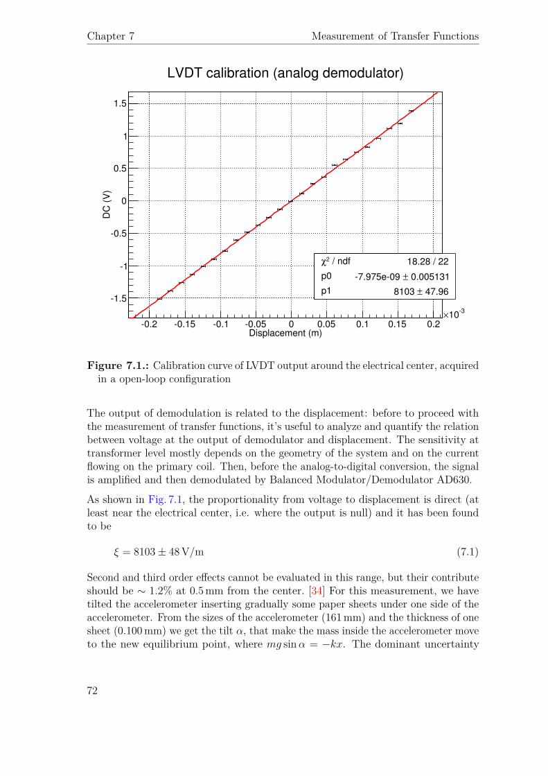
Chapter 7 Measurement of Transfer Functions

Displacement (m)­0.2 ­0.15 ­0.1 ­0.05 0 0.05 0.1 0.15 0.2

­310×

DC

(V

)

­1.5

­1

­0.5

0

0.5

1

1.5

/ ndf 2χ 18.28 / 22

p0 0.005131± ­7.975e­09

p1 47.96± 8103

/ ndf 2χ 18.28 / 22

p0 0.005131± ­7.975e­09

p1 47.96± 8103

LVDT calibration (analog demodulator)

Figure 7.1.: Calibration curve of LVDT output around the electrical center, acquiredin a open-loop configuration

The output of demodulation is related to the displacement: before to proceed withthe measurement of transfer functions, it’s useful to analyze and quantify the relationbetween voltage at the output of demodulator and displacement. The sensitivity attransformer level mostly depends on the geometry of the system and on the currentflowing on the primary coil. Then, before the analog-to-digital conversion, the signalis amplified and then demodulated by Balanced Modulator/Demodulator AD630.

As shown in Fig. 7.1, the proportionality from voltage to displacement is direct (atleast near the electrical center, i.e. where the output is null) and it has been foundto be

ξ = 8103± 48V/m (7.1)

Second and third order effects cannot be evaluated in this range, but their contributeshould be ∼ 1.2% at 0.5mm from the center. [34] For this measurement, we havetilted the accelerometer inserting gradually some paper sheets under one side of theaccelerometer. From the sizes of the accelerometer (161mm) and the thickness of onesheet (0.100mm) we get the tilt α, that make the mass inside the accelerometer moveto the new equilibrium point, where mg sinα = −kx. The dominant uncertainty

72

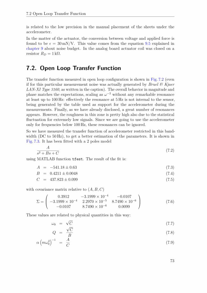
7.2 Open Loop Transfer Function

is related to the low precision in the manual placement of the sheets under theaccelerometer.In the matter of the actuator, the conversion between voltage and applied force isfound to be ε = 30mN/V. This value comes from the equation 9.5 explained inchapter 9 about noise budget. In the analog board actuator coil was closed on aresistor RD = 1 kΩ.

7.2. Open Loop Transfer Function

The transfer function measured in open loop configuration is shown in Fig. 7.2 (evenif for this particular measurement noise was actually generated by Bruel & KjaerLAN-XI Type 3160, as written in the caption). The overall behavior in magnitude andphase matches the expectations, scaling as ω−2 without any remarkable resonanceat least up to 100Hz: effectively the resonance at 5Hz is not internal to the sensor,being generated by the table used as support for the accelerometer during themeasurements. Finally, as we have already disclosed, a great number of resonancesappears. However, the roughness in this zone is pretty high also due to the statisticalfluctuation for extremely low signals. Since we are going to use the accelerometeronly for frequencies below 100Hz, these resonances can be ignored.So we have measured the transfer function of accelerometer restricted in this band-width (DC to 50Hz), to get a better estimation of the parameters. It is shown inFig. 7.3. It has been fitted with a 2 poles model

A

s2 +Bs+ C(7.2)

using MATLAB function tfest. The result of the fit is:

A = −541.18± 0.63 (7.3)B = 0.4211± 0.0048 (7.4)C = 437.823± 0.099 (7.5)

with covariance matrix relative to (A,B,C)

Σ =

0.3912 −3.1999× 10−4 −0.0107−3.1999× 10−4 2.2970× 10−5 8.7490× 10−6

−0.0107 8.7490× 10−6 0.0099

(7.6)

These values are related to physical quantities in this way:

ω0 =√C (7.7)

Q =√C

B(7.8)

α(mω2

0

)−1= A

C(7.9)

73

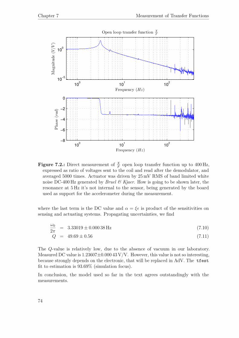
Chapter 7 Measurement of Transfer Functions

100

101

102

10−5

100

Open loop transfer function XF

Frequency (Hz)

Magnitude(V

/V)

100

101

102

−8

−6

−4

−2

0

Frequency (Hz)

Phase

(rad)

Figure 7.2.: Direct measurement of XF

open loop transfer function up to 400Hz,expressed as ratio of voltages sent to the coil and read after the demodulator, andaveraged 5000 times. Actuator was driven by 25mV RMS of band limited whitenoise DC-400Hz generated by Bruel & Kjaer. How is going to be shown later, theresonance at 5Hz it’s not internal to the sensor, being generated by the boardused as support for the accelerometer during the measurement.

where the last term is the DC value and α = ξε is product of the sensitivities onsensing and actuating systems. Propagating uncertainties, we find

ω0

2π = 3.33019± 0.000 38Hz (7.10)

Q = 49.69± 0.56 (7.11)

The Q-value is relatively low, due to the absence of vacuum in our laboratory.Measured DC value is 1.23607±0.000 43V/V. However, this value is not so interesting,because strongly depends on the electronic, that will be replaced in AdV. The tfestfit to estimation is 93.69% (simulation focus).In conclusion, the model used so far in the text agrees outstandingly with themeasurements.

74

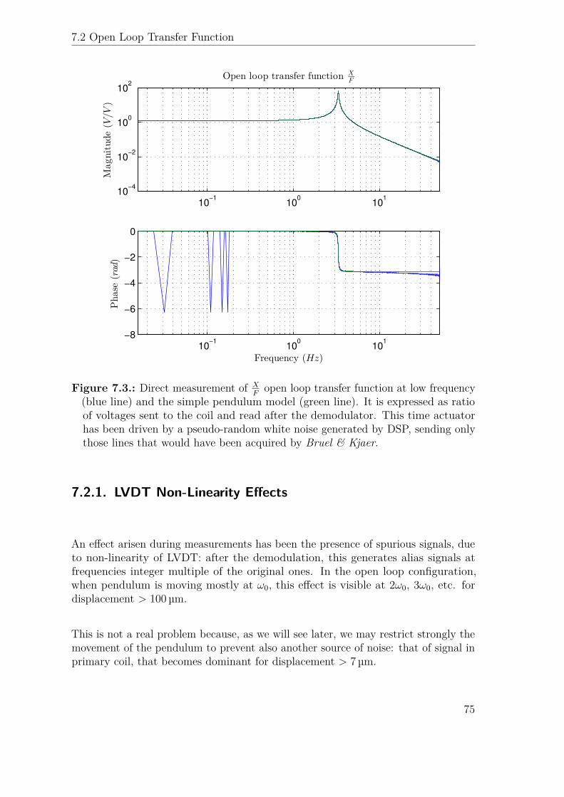
7.2 Open Loop Transfer Function

10−1

100

101

10−4

10−2

100

102

Open loop transfer function XF

Magnitude(V

/V)

10−1

100

101

−8

−6

−4

−2

0

Frequency (Hz)

Phase

(rad)

Figure 7.3.: Direct measurement of XF

open loop transfer function at low frequency(blue line) and the simple pendulum model (green line). It is expressed as ratioof voltages sent to the coil and read after the demodulator. This time actuatorhas been driven by a pseudo-random white noise generated by DSP, sending onlythose lines that would have been acquired by Bruel & Kjaer.

7.2.1. LVDT Non-Linearity Effects

An effect arisen during measurements has been the presence of spurious signals, dueto non-linearity of LVDT: after the demodulation, this generates alias signals atfrequencies integer multiple of the original ones. In the open loop configuration,when pendulum is moving mostly at ω0, this effect is visible at 2ω0, 3ω0, etc. fordisplacement > 100 µm.

This is not a real problem because, as we will see later, we may restrict strongly themovement of the pendulum to prevent also another source of noise: that of signal inprimary coil, that becomes dominant for displacement > 7 µm.

75

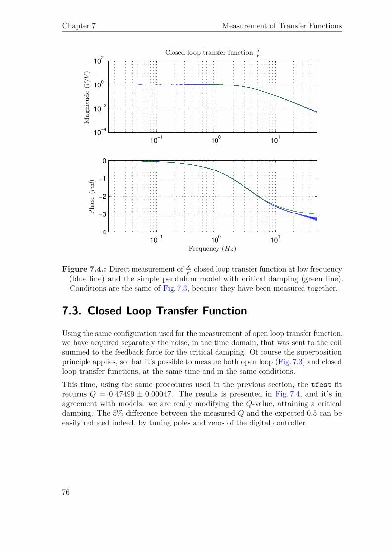
Chapter 7 Measurement of Transfer Functions

10−1

100

101

10−4

10−2

100

102

Closed loop transfer function XF

Magnitude(V

/V)

10−1

100

101

−4

−3

−2

−1

0

Frequency (Hz)

Phase

(rad)

Figure 7.4.: Direct measurement of XFclosed loop transfer function at low frequency

(blue line) and the simple pendulum model with critical damping (green line).Conditions are the same of Fig. 7.3, because they have been measured together.

7.3. Closed Loop Transfer Function

Using the same configuration used for the measurement of open loop transfer function,we have acquired separately the noise, in the time domain, that was sent to the coilsummed to the feedback force for the critical damping. Of course the superpositionprinciple applies, so that it’s possible to measure both open loop (Fig. 7.3) and closedloop transfer functions, at the same time and in the same conditions.This time, using the same procedures used in the previous section, the tfest fitreturns Q = 0.47499 ± 0.00047. The results is presented in Fig. 7.4, and it’s inagreement with models: we are really modifying the Q-value, attaining a criticaldamping. The 5% difference between the measured Q and the expected 0.5 can beeasily reduced indeed, by tuning poles and zeros of the digital controller.

76

8Digital Synthesizer and Demodulation

In this chapter we present how a Linear Variable Differential Transformer sensorworks, and how it is dimensioned inside Virgo’s accelerometers. Then, it is describedan algorithm to read the displacement using the new electronics of Advanced Virgo.

8.1. Linear Variable Differential Transformers

A LVDT consists of three solenoidal coils, placed end-to-end around a tube. The coilat the center is the primary coil, and the two outer coils are the called secondarycoils. A cylindrical ferromagnetic core, attached to the object whose position is tobe measured, is free to move along the axis of the tube.1 A carrier sine wave

Vp (t) = sin (Ωt) (8.1)

at Ω = 2π · 50 kHz with unitary amplitude, drives the primary and causes a voltageto be induced in each secondary. The output of our device is the difference of thesetwo voltages, and it can be written as

Vs (t) = A (t) sin (Ωt+ ϕ) (8.2)

where A (t) is the signal directly proportional to the displacement (at least near tothe center) and ϕ is a - usually small - primary to secondary coil phase shift. Inpractice, phase shift is almost certain to exist in the return signal due to the effect ofstray capacitance in the transducer and connecting leads, as well as from toleranceand drift effects associated with analog components in the signal path. [35]

1Actually, in accelerometer LVDT, there is no ferromagnetic core: the primary coil is attachedto the external structure, while secondary coils are integral with the pendulum. In this way,vacuum is used as medium, because of the incompatibility of a standard ferromagnetic corewith the ultra high vacuum of Virgo.

77

Chapter 8 Digital Synthesizer and Demodulation

8.1.1. Operation of a Transformer

Let’s see in details how a LVDT works. This will be useful later for the analysis ofthe propagation of noise from primary coil to secondary coils.

According to Faraday’s law of induction, voltage E induced in a coil made by Nturns is given by

E = −N ∂Φ∂t

(8.3)

where Φ is the magnetic flux through the loop. In the case of LVDT, magnetic fieldB (z, r, t) is induced by the current flowing in primary coil: it’s value is symmetricwith respect to the coil axis z, and so depends only on z and on the distance fromthe axis r =

√x2 + y2 (where x and y are directions orthogonal to z). The magnetic

flux through a secondary coil of radius R is

Φ (z, t) =ˆ R

0~B (z, r, t) · n2πrdr (8.4)

The computation of B, and then of its flux, is complicated because it involves ellipticintegrals. Omitting details, the z component of B, Bz = ~B · n, is given by

Bz (z, r, t) = i (t)µo2a

1π√q

(K(k) + (−α2 − β2 + 1)E(k)

q − 4α

)

where:

• i (t) is current in the wire;

• a radius of the current loop;

• α = ra; β = x

a; q = (α + 1)2 + β2; k =

√4αq

;

• K(k) and E(k) are complete elliptic integral of the first kind and completeelliptic integral of the second kind, respectively.

Since in a transformer the flux can be written as Φ = PNpIp, where P is thepermeance2 and NpIp is the current-turns of the primary coil, we can figure out thatpermeance and flux are functions of the distance between coils: if we let this distancevariate during time, then signals are differently induced in each secondary coil. Anumerical computation (presented in Fig. 8.1) shows that a value z0 exists, such thatthe derivative ∂P

∂zis maximized for z = ±z0, with value δP0. Those at z = ±z0 are

of course the best places where to put the secondary coils in a LVDT in order toobtain the best SNR, because a perturbation in z would produce the maximum effecton the voltage induced in secondary coils. For the Virgo horizontal accelerometers,

2The SI unit of magnetic permeance is "webers per ampere-turn", that is WbA−1.

78

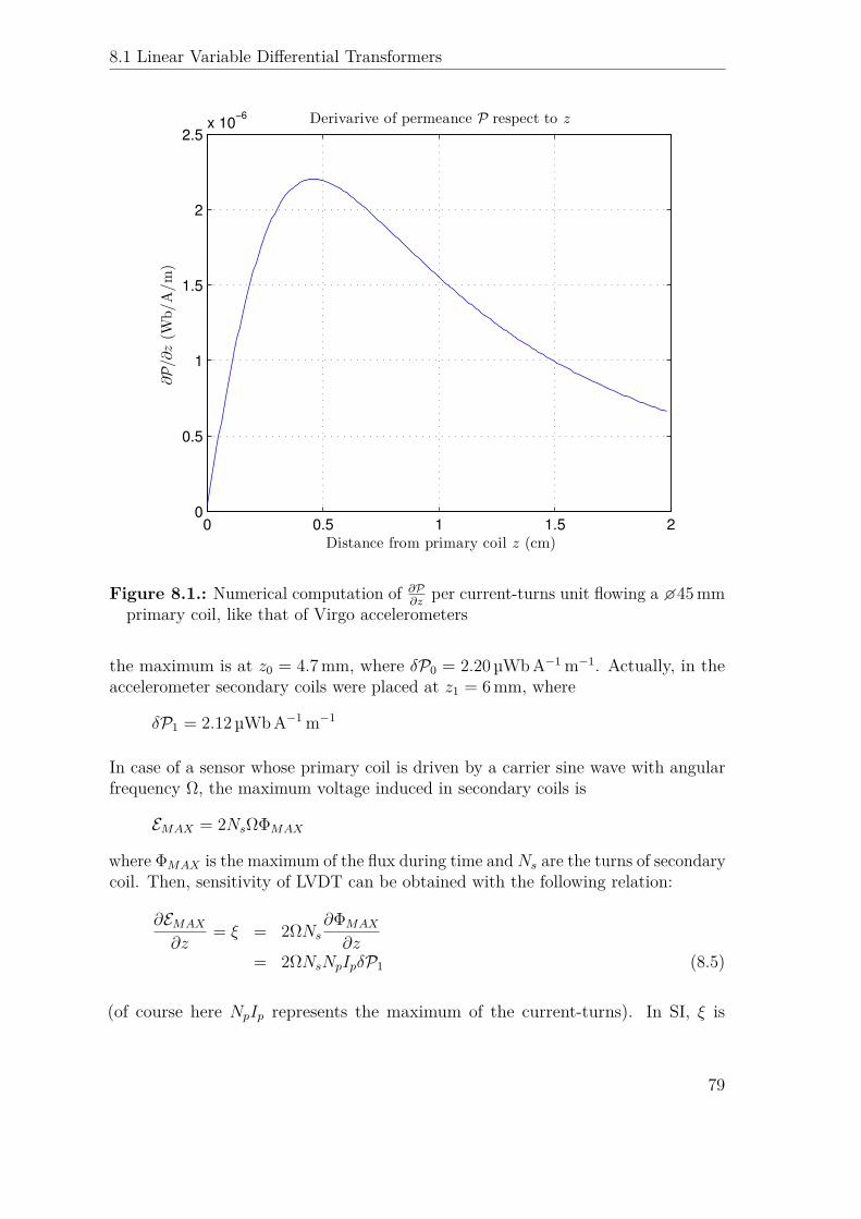
8.1 Linear Variable Differential Transformers

0 0.5 1 1.5 20

0.5

1

1.5

2

2.5x 10

−6 Derivarive of permeance P respect to z

∂P/∂z(W

b/A/m)

Distance from primary coil z (cm)

Figure 8.1.: Numerical computation of ∂P∂z

per current-turns unit flowing a 45mmprimary coil, like that of Virgo accelerometers

the maximum is at z0 = 4.7mm, where δP0 = 2.20 µWbA−1 m−1. Actually, in theaccelerometer secondary coils were placed at z1 = 6mm, where

δP1 = 2.12 µWbA−1 m−1

In case of a sensor whose primary coil is driven by a carrier sine wave with angularfrequency Ω, the maximum voltage induced in secondary coils is

EMAX = 2NsΩΦMAX

where ΦMAX is the maximum of the flux during time andNs are the turns of secondarycoil. Then, sensitivity of LVDT can be obtained with the following relation:

∂EMAX

∂z= ξ = 2ΩNs

∂ΦMAX

∂z= 2ΩNsNpIpδP1 (8.5)

(of course here NpIp represents the maximum of the current-turns). In SI, ξ is

79

Chapter 8 Digital Synthesizer and Demodulation

expressed as V/m. In our sensor these variables assume the following values:

Ω = 2π · 50 kHzNs = 450Np = 41

NpIp = 1.14A

In this conditions, according to 8.5, the sensitivity of Virgo accelerometer LVDT is

ξ = 610V/m (8.6)

where voltage are measured at the maximum during a period.

8.2. Demodulation of the LVDT Signal

A demodulator allows us to extract A (t) from Vs (t): in essence, it takes the outputsignal, then multiplies it by the reference signal sin (Ωt+ ϕ0) - that, if need be, canbe delayed by an arbitrary phase ϕ0 - and, eventually, integrates it over a specifiedtime. Analytically,

I0 (t) = A (t) sin (Ωt+ ϕ) · sin (Ωt+ ϕ0)

= A (t)2 [cos (∆ϕ)− cos (2Ωt+ ϕ+ ϕ0)] (8.7)

where we have defined

∆ϕ = ϕ− ϕ0

In the same way, using the orthogonality of sine and cosine functions, it is possible toget an another, independent signal by multiplying by cos (Ωt+ ϕ0), i.e. the referencewave shifted by π/2:

Q0 (t) = A (t) sin (Ωt+ ϕ) · cos (Ωt+ ϕ0)

= A (t)2 [sin (∆ϕ) + sin (2Ωt+ ϕ+ ϕ0)] (8.8)

In both cases, the resulting signal is A, multiplied by the sum of a DC signal anda signal at twice the reference signal frequency Ω. If the bandwidth of A is muchsmaller than Ω, a proper low-pass filter - with gain 2 at low frequencies - applied tothese two signals finally lets us to obtain

I (t) = A (t) cos (∆ϕ) (8.9)Q (t) = A (t) sin (∆ϕ)

80

8.2 Demodulation of the LVDT Signal

i.e. two signals both proportional to A (t) and to a constant. This is the principleof a lock-in amplifier, also known as a phase-sensitive detector for this reason.The letters I and Q are used in electrical engineering to represent two amplitude-modulated sinusoids that are offset in phase by one-quarter cycle: they stand forin-phase and quadrature components, respectively.To get the maximum SNR from the in-phase component I, we have to maximizethe coefficient cos (∆ϕ). Obviously, the optimal case shows up for ∆ϕ = 0, that canbe achieved by tuning ϕ0 = ϕ. Nevertheless, we don’t know a priori the value of ϕ.Luckily, a slightly non-zero ∆ϕ implies only a second-order effect in I, so that thetuning does not require an extreme precision.In our system, the simplest way to measure the phase shift is

∆ϕ = tan−1(Q (t)I (t)

)(8.10)

However this is not a good approach, as the calculation of tan−1 in double precisionfloating point takes a long time to the DSP (∼ 300 clock cycles), and also becauseI (t) often goes through zero. This identity is an alternative approach:

I (t) ·Q (t)I2 (t) +Q2 (t) = A2 (t) sin (∆ϕ) cos (∆ϕ)

A2 (t) = sin (2∆ϕ)2 (8.11)

The main advantage is to have the denominator A2 (t) always greater or equal to 0,making the computation of the division safer. Furthermore,

sin (2∆ϕ)2 = ∆ϕ

at the first order in ∆ϕ: this means that it’s possible to avoid the calculation ofsin−1 (as laborious as tan−1).

8.2.1. Effects of a Quadrature Term

In addition to phase shift, that is relatively little annoying, a real LVDT shows alsoanother tedious effect: actually, in the secondary coils voltage 8.2 a term B appears,in quadrature to A:

Vs (t) = A (t) sin (Ωt+ ϕ) +B (t) cos (Ωt+ ϕ) (8.12)

In this backdrop, we need to rewrite equation 8.7 and 8.8:

I0 (t) = [A (t) sin (Ωt+ ϕ) +B (t) cos (Ωt+ ϕ)] · sin (Ωt+ ϕ0)

= A (t)2 [cos (∆ϕ)− cos (2Ωt+ ϕ+ ϕ0)]

−B (t)2 [sin (∆ϕ)− sin (2Ωt+ ϕ+ ϕ0)]

81

Chapter 8 Digital Synthesizer and Demodulation

and

Q0 (t) = [A (t) sin (Ωt+ ϕ) +B (t) cos (Ωt+ ϕ)] · cos (Ωt+ ϕ0)

= A (t)2 [sin (∆ϕ) + sin (2Ωt+ ϕ+ ϕ0)]

+B (t)2 [cos (∆ϕ) + cos (2Ωt+ ϕ+ ϕ0)]

These, after the same low-pass filter, become

I (t) = A (t) cos (∆ϕ)−B (t) sin (∆ϕ) (8.13)Q (t) = A (t) sin (∆ϕ) +B (t) cos (∆ϕ)

or equivalently, in matrix notation,(I (t)Q (t)

)=(

cos (∆ϕ) − sin (∆ϕ)sin (∆ϕ) cos (∆ϕ)

)(A (t)B (t)

)(8.14)

In other words, the vector (I (t) , Q (t)) is nothing more than (A (t) , B (t)) rotatedby an angle ∆ϕ. Now, we have two equations for three unknowns: there is no way tomeasure ∆ϕ by the only measure of (I (t) , Q (t)), so that it’s impossible to isolate thedisplacement signal A (t) from the quadrature term. The presence of a non-adjustedphase shift inevitably leads to a mixing of A and B on the output of the system.Fortunately, there’s no need to be discouraged: if |B| |A| (the dependence on timeis omitted from now on), the contribution of the quadrature term can be actuallyneglected, in order to use either equation 8.10 or 8.11 to measure ∆ϕ. For example,defining

r = B

A

equation 8.11 using I and Q of 8.13 would become

I ·QI2 +Q2 = sin(2∆ϕ) + 2r cos(2∆ϕ)− r2 sin(2∆ϕ)

2 (1 + r2)

whose denominator is strictly greater than 0 if r 6= 0. At the first order in r and in∆ϕ, it shrinks to

I ·QI2 +Q2 = ∆ϕ+ r (8.15)

In conclusion, this ratio can be used for calculate ∆ϕ in adequate conditions. Fur-thermore the denominator is always positive, and a division by zero never occurs.The error introduced by the quadrature signal B is just r.

82

8.3 An Algorithm to Demodulate with Phase Locking

Now, the problem becomes how to get r → 0, i.e. |B| |A|. Even if B is relativelysmall and constant over the time, and independent from the displacement, we don’tknow the initial size of the signal A, that could also be zero. Qualitatively, we canapply a relatively strong force to the mass through the coil actuator, in order toget a displacement x− x0 as big as possible: this will increase A while, at the sametime, B remains constant. Then, we perform a measurement of ϕ, set ϕ0 = ϕ andeventually release the force. At that point, we’ll have I = A and Q = B. This canbe achieved by a finite-state machine implemented in the FPGA.

8.3. An Algorithm to Demodulate with PhaseLocking

Today, digital techniques can be applied in order to automate this tuning. Inparticular, a Phase-Locked Loop (PLL) is a control system that generates anoutput signal whose phase is related to the phase of an input signal. We can usethis technique to measure the phase shift and then to tune the oscillator used forthe demodulation with a phase ϕ0 = ϕ.A digital PLL-based loop can be implemented in FPGA, to perform amplitudedemodulation using the relation in 8.15 for a smart measurement of ϕ and thusallowing to get the maximum SNR from the in-phase component I. Such a systemcan be used to read LVDT, both those inside the accelerometer and the others usedin the Superattenuator inertial control.The schematic diagram is depicted in Fig. 8.2. The principle is quite simple: afterthe reconstruction of I and Q from LVDT secondary coils, they are combined to get∆ϕ. This value passes through an integrator, that slowly changes the initial phaseϕ0 of a sine-cosine wave generator used in the demodulation. Supposing r → 0, astime passes ϕ0 tends to ϕ, giving ∆ϕ→ 0. At this point the system is stable: weget I → A, Q→ B, and ϕ0 that is a direct measurement of time shift.First of all the logic has been tested in MATLAB and Simulink, simulating a discretetime model. This has been done mostly to check the performance and to tune theparameters. The result of a simulation with a 1Hz signal, B = 0 and ϕ = 1.4 rad ispresented in Fig. 8.3: as expected, while the feedback phase ϕ0 tends to the rightvalue, I → A and Q→ 0.Eventually, I have developed a project in Quartus II 13.1.0, both writing VHDL codeand using schematic files, to be implemented in Advanced Virgo electronics. Dueto the complex handling of floating point values in a FPGA, all the vectors havebeen treated as signed and/or unsigned integers, using numeric_std package. Onthe one hand this simplifies several things: for example, the output of ADC belongto this data type, and so no conversions are needed; it is also trivial to performmultiplication and division by powers of two. On the other hand, we need to payattention to the number of bits used in the arithmetics, to avoid losses of precision.

83

Chapter 8 Digital Synthesizer and Demodulation

LVDT

×

×

low pass

low pass

I·QI2+Q2

integrator50 kHz NCO50 kHz NCO

Vs

I0

Q0

I

Q

∆ϕ

ϕ0sin (Ωt+ ϕ0)

cos (Ωt+ ϕ0)

Vp = sin (Ωt)

Figure 8.2.: Schematic diagram of the PLL-based demodulation with phase locking

Numerically Controlled Oscillator

50 kHz NCOϕ0 sin (Ωt+ ϕ0)

The central block is the Numerically Controlled Oscillator (NCO): this term indicatesa digital signal generator which creates a synchronous (i.e. clocked), discrete-time,discrete-valued representation of a waveform. A first NCO is used to generate twocoherent 50 kHz sinusoidal waves, phase-shifted by π/2 each other, that are usedfor the demodulation. Another identical and independent NCO is used to drive theprimary coil of LVDT.

An NCO generally consists of two parts:

• A Phase Accumulator (PA), which adds a frequency control value to the valueheld at its output at each clock sample.

• A Phase-to-Amplitude Converter (PAC), which uses the PA output word asan index into a waveform Look-Up Table (LUT), to provide a correspondingamplitude sample. Sometimes interpolation is used with the look-up table toprovide better accuracy and reduce phase error noise.

I have written a VHDL code, based on the excellent LGPL-licensed project DDSSynthesizer, developed since 2008 by Martin Kumm. [36] Let’s see the essence of thealgorithm, whose schematic is in Fig. 8.4, looking at some extracts from the VHDLcode.

1 −− phase accumulators2 ftw_accu <= ftw_accu + ftw_i ;

84

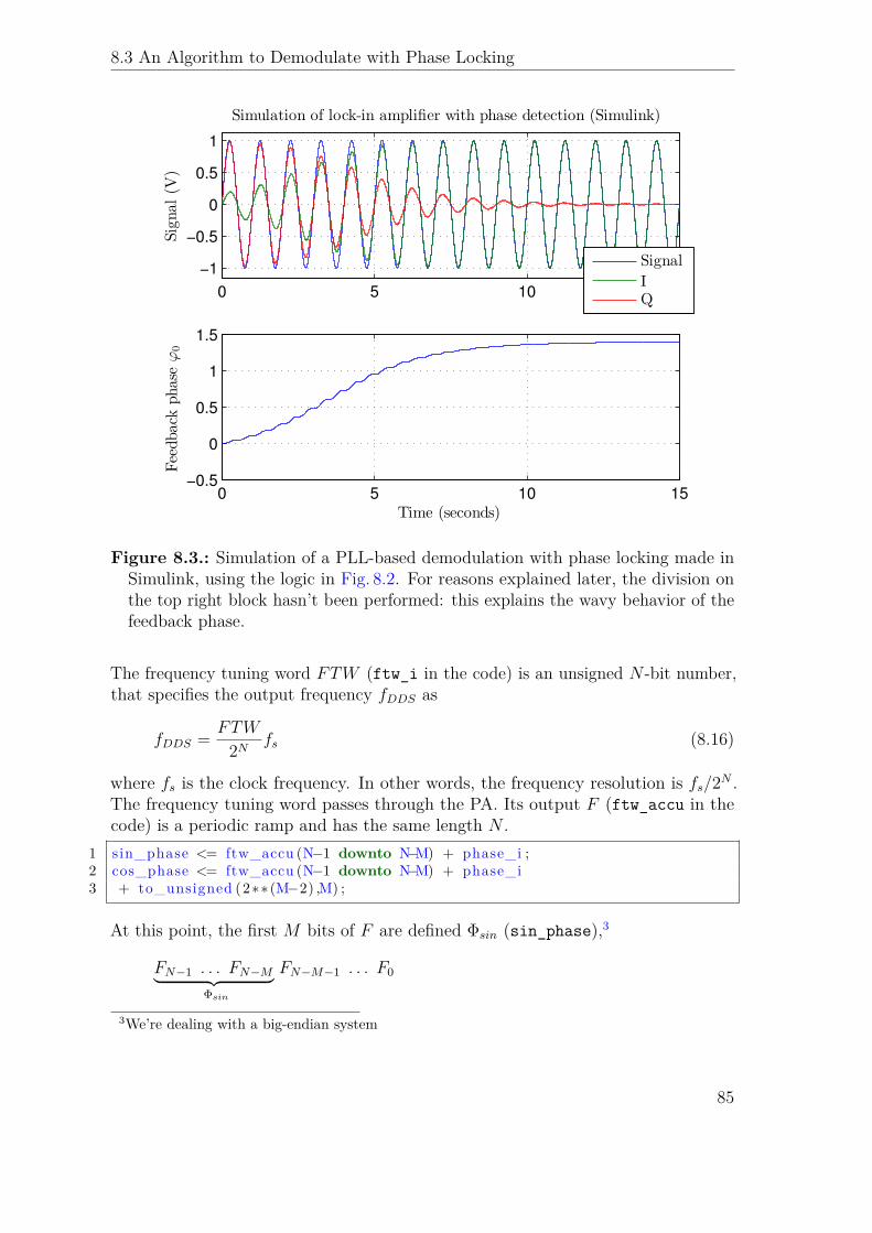
8.3 An Algorithm to Demodulate with Phase Locking

0 5 10 15

−1

−0.5

0

0.5

1

Signal(V

)

Simulation of lock-in amplifier with phase detection (Simulink)

Signal

IQ

0 5 10 15−0.5

0

0.5

1

1.5

Time (seconds)

Feedback

phase

ϕ0

Figure 8.3.: Simulation of a PLL-based demodulation with phase locking made inSimulink, using the logic in Fig. 8.2. For reasons explained later, the division onthe top right block hasn’t been performed: this explains the wavy behavior of thefeedback phase.

The frequency tuning word FTW (ftw_i in the code) is an unsigned N -bit number,that specifies the output frequency fDDS as

fDDS = FTW

2N fs (8.16)

where fs is the clock frequency. In other words, the frequency resolution is fs/2N .The frequency tuning word passes through the PA. Its output F (ftw_accu in thecode) is a periodic ramp and has the same length N .

1 sin_phase <= ftw_accu (N−1 downto N−M) + phase_i ;2 cos_phase <= ftw_accu (N−1 downto N−M) + phase_i3 + to_unsigned (2∗∗ (M−2) ,M) ;

At this point, the first M bits of F are defined Φsin (sin_phase),3

FN−1 . . . FN−M︸ ︷︷ ︸Φsin

FN−M−1 . . . F0

3We’re dealing with a big-endian system

85

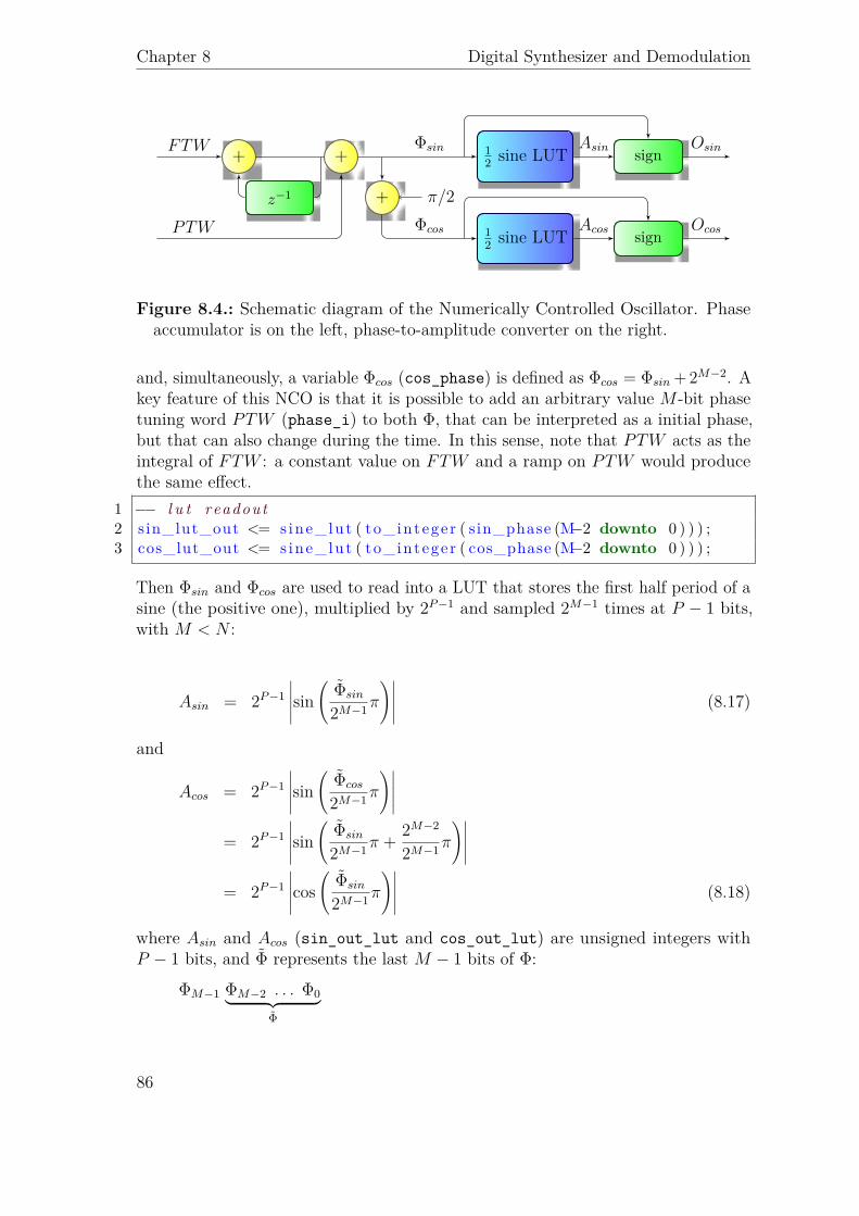
Chapter 8 Digital Synthesizer and Demodulation

+

z−1

+ 12 sine LUT

+ π/2

12 sine LUT

sign

sign

FTW

PTW

Φsin

Φcos

Asin

Acos

Osin

Ocos

Figure 8.4.: Schematic diagram of the Numerically Controlled Oscillator. Phaseaccumulator is on the left, phase-to-amplitude converter on the right.

and, simultaneously, a variable Φcos (cos_phase) is defined as Φcos = Φsin + 2M−2. Akey feature of this NCO is that it is possible to add an arbitrary value M -bit phasetuning word PTW (phase_i) to both Φ, that can be interpreted as a initial phase,but that can also change during the time. In this sense, note that PTW acts as theintegral of FTW : a constant value on FTW and a ramp on PTW would producethe same effect.

1 −− l u t readout2 sin_lut_out <= s ine_lut ( to_integer ( sin_phase (M−2 downto 0 ) ) ) ;3 cos_lut_out <= s ine_lut ( to_integer ( cos_phase (M−2 downto 0 ) ) ) ;

Then Φsin and Φcos are used to read into a LUT that stores the first half period of asine (the positive one), multiplied by 2P−1 and sampled 2M−1 times at P − 1 bits,with M < N :

Asin = 2P−1∣∣∣∣∣sin

(Φsin

2M−1π

)∣∣∣∣∣ (8.17)

and

Acos = 2P−1∣∣∣∣∣sin

(Φcos

2M−1π

)∣∣∣∣∣= 2P−1

∣∣∣∣∣sin(

Φsin

2M−1π + 2M−2

2M−1π

)∣∣∣∣∣= 2P−1

∣∣∣∣∣cos(

Φsin

2M−1π

)∣∣∣∣∣ (8.18)

where Asin and Acos (sin_out_lut and cos_out_lut) are unsigned integers withP − 1 bits, and Φ represents the last M − 1 bits of Φ:

ΦM−1 ΦM−2 . . . Φ0︸ ︷︷ ︸Φ

86

8.3 An Algorithm to Demodulate with Phase Locking

Only half a period of sine is stored because of the property sin (x) = − sin (x+ π).4The first two bits of Φsin and Φcos represents the quadrant relative the angle, thatis related to the sign of sine and cosine: the sine is positive in the first and in thesecond ones, while the cosine in the first and in the forth ones. Furthermore, thephase of cosine is one quadrant ahead that of sine: this is why we define only one2-bit unsigned integer signal quadrant, relative to the sine:

1 quadrant <= sin_phase (M−1 downto M−2);

The remaining last N −M bits of F are discarded in the PAC, as they are neededonly for the frequency tuning. They could be used for an eventual interpolation, toprovide better accuracy and reduce phase error noise.

In conclusion, the outputs of NCO are two P -bit signed integers, Osin (sin_o) andOcos (cos_o), that consist of A with the adjusted sign, and that are written justafter the clock rising edge:

1 −− w r i t i n g output ( quadrant i s t h a t o f s in )2 sin_o <= sin_lut_out_delay3 when ( quadrant_2delay = " 00 " or quadrant_2delay = " 01 " )4 else sin_lut_out_inv_delay ;5 cos_o <= cos_lut_out_delay6 when ( quadrant_2delay = " 00 " or quadrant_2delay = " 11 " )7 else cos_lut_out_inv_delay ;

taking, from the previous iteration,1 −− updat ing quadrant memory2 quadrant_delay <= quadrant ;3 quadrant_2delay <= quadrant_delay ;45 −− updat ing output f o r the next i t e r a t i o n6 sin_lut_out_inv_delay <= to_signed (−1∗ to_integer ( sin_lut_out ) , P ) ;7 sin_lut_out_delay <= sin_lut_out ;8 cos_lut_out_inv_delay <= to_signed (−1∗ to_integer ( cos_lut_out ) , P ) ;9 cos_lut_out_delay <= cos_lut_out ;

The signals, with self-explaining suffixes _delay and _2delay, are needed to takeinto account the delays of the algorithm: the latency of this NCO is 2 clock cycles.

In the implementation used in our test, we have used N = 24, M = 10 and P = 10.Look-up tables, compatible with the code, are generated by a MATLAB script, witharbitrary M and P .

4The original Kumm’s algorithm stores only the first quarter of the period of a sine on the LUT,exploiting the property sin

(x + π

2)

= sin(−x + π

2). However, in this way the value of the

maximum of the sine is not stored in the LUT and has to be written in the code, generating anexception inside the algorithm: this problem is avoided, storing the whole first half period.

87

Chapter 8 Digital Synthesizer and Demodulation

Low Pass Filters

low passI0 I

The output of LVDT is acquired by ADC in a 24-bit value, and multiplied by the10-bit outputs of NCO to form I0 and Q0, each one with 34 bits. A low pass filter isthen needed removes the 2Ω contribution.

Instead of a simple low pass filter, we can use a property of the average. In Z-transform, the average of n samples as this form:

Y

X= 1 + z−1 + z−2 + . . .+ z−n+1

n= 1n

1− z−n1− z−1 (8.19)

that corresponds to a simple difference equation

yi = yi−1 + xi − xi−nn

(8.20)

Its sinc-like frequency response (see Fig. 8.5) has the property to have a notch in allmultiples of fc/n, when the wave has a integer number of periods under the averagingwindow.5

At this point we would like also to downsample the stream of data: ADC are read atfc = 3.84MHz, that is pretty high for our purpose. So, the strategy is the following:an accumulator averages n = 19 samples, then its output is read and the accumulatoris reset.

Why 19? Because it is the nearest integer to 19.2, which would allow to put a notchat 3.84 MHz

19.2 = 200 kHz. Choosing n = 19, the first notch is actually at fc = 202.1 kHz,that is still acceptable. And also, why do we chose 200 kHz and not 100 kHz, wherewe have the 2Ω contribution of demodulation? Because resampling the stream at100 kHz would create some aliasing in DC, as the notch has a very narrow band (lookat 8.7 and 8.8: the signal A (t) is amplitude modulated around 2Ω). This is not aproblem if we downsample at 200 kHz, because there should be only a little noise.

This step is performed by ALTACCUMULATE Quartus megafunction. Of course,this first average does not filter too much at 100 kHz: from transfer function 8.19,

5Sinc-like behavior is a direct consequence of the Fourier transform, in the analog domain, of aunit box (f (t) = a−1 if t < a else f (t) = 0, where a > 0), that is proportional to cardinal sinefunction sincx = sin x

x .

88

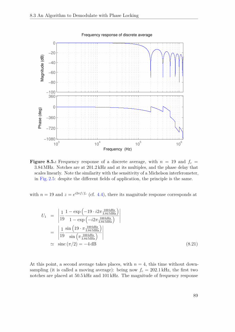
8.3 An Algorithm to Demodulate with Phase Locking

−100

−80

−60

−40

−20

0M

agnitude (

dB

)

Frequency response of discrete average

Frequency (Hz)

103

104

105

106

−1080

−720

−360

0

360

Phase (

deg)

Figure 8.5.: Frequency response of a discrete average, with n = 19 and fc =3.84MHz. Notches are at 201.2 kHz and at its multiples, and the phase delay thatscales linearly. Note the similarity with the sensitivity of a Michelson interferometer,in Fig. 2.5: despite the different fields of application, the principle is the same.

with n = 19 and z = ei2πf/fc (cf. 4.4), there its magnitude response corresponds at

U1 =∣∣∣∣∣∣ 119

1− exp(−19 · i2π 100 kHz

3.84 MHz

)1− exp

(−i2π 100 kHz

3.84 MHz

)∣∣∣∣∣∣

=∣∣∣∣∣∣ 119

sin(19 · π 100 kHz

3.84 MHz

)sin

(π 100 kHz

3.84 MHz

)∣∣∣∣∣∣

' sinc (π/2) = −4 dB (8.21)

At this point, a second average takes places, with n = 4, this time without down-sampling (it is called a moving average): being now fc = 202.1 kHz, the first twonotches are placed at 50.5 kHz and 101 kHz. The magnitude of frequency response

89

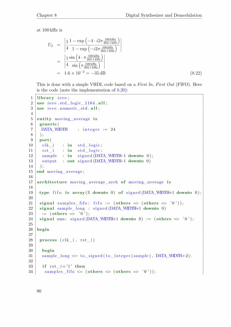
Chapter 8 Digital Synthesizer and Demodulation

at 100 kHz is

U2 =∣∣∣∣∣∣14

1− exp(−4 · i2π 100 kHz

202.1 kHz

)1− exp

(−i2π 100 kHz

202.1 kHz

)∣∣∣∣∣∣

=∣∣∣∣∣∣14

sin(4 · π 100 kHz

202.1 kHz

)sin

(π 100 kHz

202.1 kHz

)∣∣∣∣∣∣

= 1.6× 10−2 = −35 dB (8.22)

This is done with a simple VHDL code based on a First In, First Out (FIFO). Hereis the code (note the implementation of 8.20):

1 l ibrary i e e e ;2 use i e e e . std_logic_1164 . a l l ;3 use i e e e . numeric_std . a l l ;45 entity moving_average i s6 generic (7 DATA_WIDTH : i n t e g e r := 248 ) ;9 port (

10 c lk_i : in s td_log i c ;11 r s t_ i : in s td_log i c ;12 sample : in s igned (DATA_WIDTH−1 downto 0 ) ;13 output : out s igned (DATA_WIDTH−1 downto 0)14 ) ;15 end moving_average ;1617 architecture moving_average_arch of moving_average i s1819 type f i f o i s array (3 downto 0) of s igned (DATA_WIDTH+1 downto 0 ) ;2021 signal sample s_f i f o : f i f o := ( others => ( others => ’ 0 ’ ) ) ;22 signal sample_long : s igned (DATA_WIDTH+1 downto 0)23 := ( others => ’ 0 ’ ) ;24 signal sum : s igned (DATA_WIDTH+1 downto 0) := ( others => ’ 0 ’ ) ;2526 begin2728 process ( clk_i , r s t_ i )2930 begin31 sample_long <= to_signed ( to_integer ( sample ) , DATA_WIDTH+2);3233 i f r s t_ i = ’1 ’ then34 sample s_f i f o <= ( others => ( others => ’ 0 ’ ) ) ;

90

8.3 An Algorithm to Demodulate with Phase Locking

35 sum <= ( others => ’ 0 ’ ) ;3637 e l s i f r i s ing_edge ( c lk_i ) then38 −− d i f f e r e n c e equat ion o f average :39 sum <= sum + sample_long − sample s_f i f o ( 0 ) ;40 −− s l i d i n g o f FIFO:41 sample s_f i f o <= sample_long & sample s_f i f o (3 downto 1 ) ;42 end i f ;4344 end process ;45 −− d i v i s i o n by 4 , cropping the l a s t 2 d i g i t s o f sum :46 output <= sum(DATA_WIDTH+1 downto 2 ) ;4748 end moving_average_arch ;

In the last step of the block, a first order digital low pass filter, with cutoff angularfrequency of 100 rad/s, is implemented6 to further clean the 2Ω signal. Its differenceequation and transfer function are7

yn = (1− α)xn + α · yn−1Y

X= 1− α

1− α · z−1 (8.23)

The term (1− α) in front of xn and at numerator in the second line is needed tohave unity gain in DC. The value α determines the time constant τ of the filter, withthe relation

logα = −Tτ

(8.24)

where T is the sampling period, (202.1 kHz)−1 = 4.9 µs in our case. For a cutoffangular frequency of 100 rad/s, τ = (100 rad/s)−1 = 10ms, we need

logα = −4.9 µs10ms ⇒ α = 0.999505 (8.25)

that is very close to the ratio 20472048 (within 0.001%), thus allowing a simple implemen-

tation at 12 bits in the FPGA.6Even if 100 rad/s ∼= 16Hz is smaller than the bandwidth of the accelerometer, it is enough forthe measurement of ϕ.

7Note that such a filter does not correspond to a continuous time filter through bilinear transfor-mation. Actually this transformation is called impulse invariance, designing discrete-time filtersfrom continuous-time filters, in which the impulse response of the continuous-time system issampled to produce the impulse response of the discrete-time system. If obtained from a firstorder continuous-time low pass filter using bilinear transformation, the transfer function in 8.23would have an additional term in z−1 at the numerator, so that the digital filter would requirean additional sum, of a term proportional to xn−1. Even if the attenuation at high frequencieswould be better, for the purposes of this system it is enough.

91

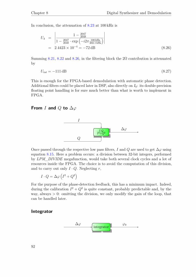
Chapter 8 Digital Synthesizer and Demodulation

In conclusion, the attenuation of 8.23 at 100 kHz is

U3 =∣∣∣∣∣∣ 1− 2047

2048

1− 20472048 · exp

(−i2π 100 kHz

202.1 kHz

)∣∣∣∣∣∣

= 2.4423× 10−4 = −72 dB (8.26)

Summing 8.21, 8.22 and 8.26, in the filtering block the 2Ω contribution is attenuatedby

Utot = −111 dB (8.27)

This is enough for the FPGA-based demodulation with automatic phase detection.Additional filters could be placed later in DSP, also directly on I0: its double-precisionfloating point handling is for sure much better than what is worth to implement inFPGA.

From I and Q to ∆ϕ

I·QI2+Q2

I

Q

∆ϕ

Once passed through the respective low pass filters, I and Q are used to get ∆ϕ usingequation 8.15. Here a problem occurs: a division between 32-bit integers, performedby LPM_DIVIDE megafunction, would take both several clock cycles and a lot ofresources inside the FPGA. The choice is to avoid the computation of this division,and to carry out only I ·Q. Neglecting r,

I ·Q = ∆ϕ(I2 +Q2

)For the purpose of the phase-detection feedback, this has a minimum impact. Indeed,during the calibration I2 +Q2 is quite constant, probably predictable and, by theway, always > 0: omitting the division, we only modify the gain of the loop, thatcan be handled later.

Integrator

integrator∆ϕ ϕ0

92

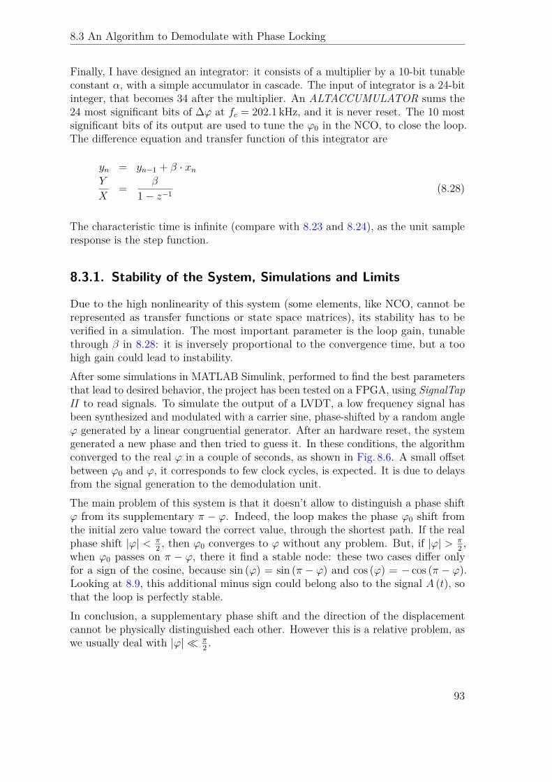
8.3 An Algorithm to Demodulate with Phase Locking

Finally, I have designed an integrator: it consists of a multiplier by a 10-bit tunableconstant α, with a simple accumulator in cascade. The input of integrator is a 24-bitinteger, that becomes 34 after the multiplier. An ALTACCUMULATOR sums the24 most significant bits of ∆ϕ at fc = 202.1 kHz, and it is never reset. The 10 mostsignificant bits of its output are used to tune the ϕ0 in the NCO, to close the loop.The difference equation and transfer function of this integrator are

yn = yn−1 + β · xnY

X= β

1− z−1 (8.28)

The characteristic time is infinite (compare with 8.23 and 8.24), as the unit sampleresponse is the step function.

8.3.1. Stability of the System, Simulations and Limits

Due to the high nonlinearity of this system (some elements, like NCO, cannot berepresented as transfer functions or state space matrices), its stability has to beverified in a simulation. The most important parameter is the loop gain, tunablethrough β in 8.28: it is inversely proportional to the convergence time, but a toohigh gain could lead to instability.After some simulations in MATLAB Simulink, performed to find the best parametersthat lead to desired behavior, the project has been tested on a FPGA, using SignalTapII to read signals. To simulate the output of a LVDT, a low frequency signal hasbeen synthesized and modulated with a carrier sine, phase-shifted by a random angleϕ generated by a linear congruential generator. After an hardware reset, the systemgenerated a new phase and then tried to guess it. In these conditions, the algorithmconverged to the real ϕ in a couple of seconds, as shown in Fig. 8.6. A small offsetbetween ϕ0 and ϕ, it corresponds to few clock cycles, is expected. It is due to delaysfrom the signal generation to the demodulation unit.The main problem of this system is that it doesn’t allow to distinguish a phase shiftϕ from its supplementary π − ϕ. Indeed, the loop makes the phase ϕ0 shift fromthe initial zero value toward the correct value, through the shortest path. If the realphase shift |ϕ| < π

2 , then ϕ0 converges to ϕ without any problem. But, if |ϕ| > π2 ,

when ϕ0 passes on π − ϕ, there it find a stable node: these two cases differ onlyfor a sign of the cosine, because sin (ϕ) = sin (π − ϕ) and cos (ϕ) = − cos (π − ϕ).Looking at 8.9, this additional minus sign could belong also to the signal A (t), sothat the loop is perfectly stable.In conclusion, a supplementary phase shift and the direction of the displacementcannot be physically distinguished each other. However this is a relative problem, aswe usually deal with |ϕ| π

2 .

93

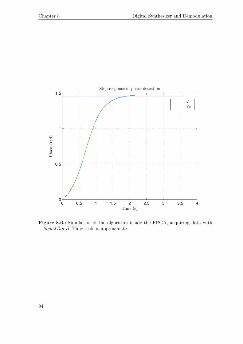
Chapter 8 Digital Synthesizer and Demodulation

0 0.5 1 1.5 2 2.5 3 3.5 40

0.5

1

1.5

Step response of phase detection

Time (s)

Phase

(rad)

ϕ

ϕ0

Figure 8.6.: Simulation of the algorithm inside the FPGA, acquiring data withSignalTap II. Time scale is approximate.

94

9Accelerometer Noise Budget

The analytical form of accelerometer SNR has been presented in equation 6.10 andshows two main sources of noise in the accelerometer: the contributions come fromthe sensors and from the actuators. A third contribution is the process noise, thatturns out to be negligible.

In this chapter the main contributes of this curve are analyzed and, eventually,compared with the noise budget of the accelerometer with the analog control.

9.1. Process Noise

In a mechanical oscillator subject to a viscous damping, thermal noise act as a noisein force with power spectral density

f 2n = 4kTmω0

Q

(see Appendix B for details). Of course the Q-value to be used is the open-loop one(Q ∼ 200), because the Q = 0.5 induced by the feedback doesn’t correspond to areal loss of energy for friction (we could define it “cold friction”). This force acts likethe feedback force, passing through the transfer function 6.8.

For our pendulum, at low frequencies the equivalent noise in acceleration is

Sthermal (ω ω0) =∣∣∣∣∣6.5× 10−11m/s2

√Hz

∣∣∣∣∣2

and then decreases as ω−4.

95

Chapter 9 Accelerometer Noise Budget

9.2. Sensing Noise

9.2.1. Noise on Primary Coil

Displacement sensors are LVDT. A 50 kHz sine wave signal is generated by FPGAusing the 10-bits digital synthesizer presented in the previous section. The numericalnoise is negligible, and in case can be easily reduced by increasing the number ofbits. This carrier wave is sent by a DAC to the primary coil. At first sight DACnoise is negligible, because if the distances between coils are identical, it inducesthe same effects on each secondary coil, that are mutually canceled. However, ifthere is an offset in the position of secondary coils, that can occur for example whenaccelerometer is subject to a tilt, then this cancellation doesn’t occur anymore andproblems can arise.Quantitatively, the mutual inductance M between primary coil and a secondary coilsatisfies the following relation (in Laplace transform) about the voltage on secondarycoil

NssΦ = MsIp + LssIs

where Lp and Ls are inductance of primary and secondary coils, respectively. Thelast term is zero in open-circuit configuration. Thus

M = NsΦIp

= NsNpΦ

NpIp= NsNpP

where P is the magnetic permeance through secondary coil, and its value at z = 6mmis P1 = 2.9× 10−8 WbA−1 (it comes from the integral of Fig. 8.1). The couplingcoefficient kps (such that |kps| ≤ 1) can be defined as

kps =

√LsLp

M

In the accelerometer, being Lp = 0.13mH and Ls = 12.4mH,[37] kps is found to be

kps = NsNpP√LpLs

= 0.42

For comparison, the coupling coefficient between secondary coils is kss ∼ 0.1, reason-ably lower due to the greater distance between coils and their smaller dimensions. [37]

96

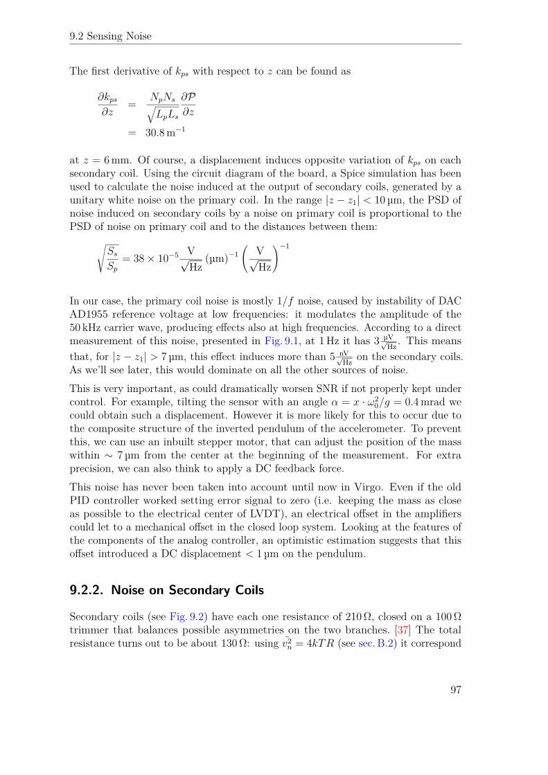
9.2 Sensing Noise

The first derivative of kps with respect to z can be found as

∂kps∂z

= NpNs√LpLs

∂P∂z

= 30.8m−1

at z = 6mm. Of course, a displacement induces opposite variation of kps on eachsecondary coil. Using the circuit diagram of the board, a Spice simulation has beenused to calculate the noise induced at the output of secondary coils, generated by aunitary white noise on the primary coil. In the range |z − z1| < 10 µm, the PSD ofnoise induced on secondary coils by a noise on primary coil is proportional to thePSD of noise on primary coil and to the distances between them:√

SsSp

= 38× 10−5 V√Hz

(µm)−1(

V√Hz

)−1

In our case, the primary coil noise is mostly 1/f noise, caused by instability of DACAD1955 reference voltage at low frequencies: it modulates the amplitude of the50 kHz carrier wave, producing effects also at high frequencies. According to a directmeasurement of this noise, presented in Fig. 9.1, at 1Hz it has 3 µV√

Hz . This meansthat, for |z − z1| > 7 µm, this effect induces more than 5 nV√

Hz on the secondary coils.As we’ll see later, this would dominate on all the other sources of noise.This is very important, as could dramatically worsen SNR if not properly kept undercontrol. For example, tilting the sensor with an angle α = x · ω2

0/g = 0.4mrad wecould obtain such a displacement. However it is more likely for this to occur due tothe composite structure of the inverted pendulum of the accelerometer. To preventthis, we can use an inbuilt stepper motor, that can adjust the position of the masswithin ∼ 7 µm from the center at the beginning of the measurement. For extraprecision, we can also think to apply a DC feedback force.This noise has never been taken into account until now in Virgo. Even if the oldPID controller worked setting error signal to zero (i.e. keeping the mass as closeas possible to the electrical center of LVDT), an electrical offset in the amplifierscould let to a mechanical offset in the closed loop system. Looking at the features ofthe components of the analog controller, an optimistic estimation suggests that thisoffset introduced a DC displacement < 1 µm on the pendulum.

9.2.2. Noise on Secondary Coils

Secondary coils (see Fig. 9.2) have each one resistance of 210 Ω, closed on a 100 Ωtrimmer that balances possible asymmetries on the two branches. [37] The totalresistance turns out to be about 130 Ω: using v2

n = 4kTR (see sec. B.2) it correspond

97

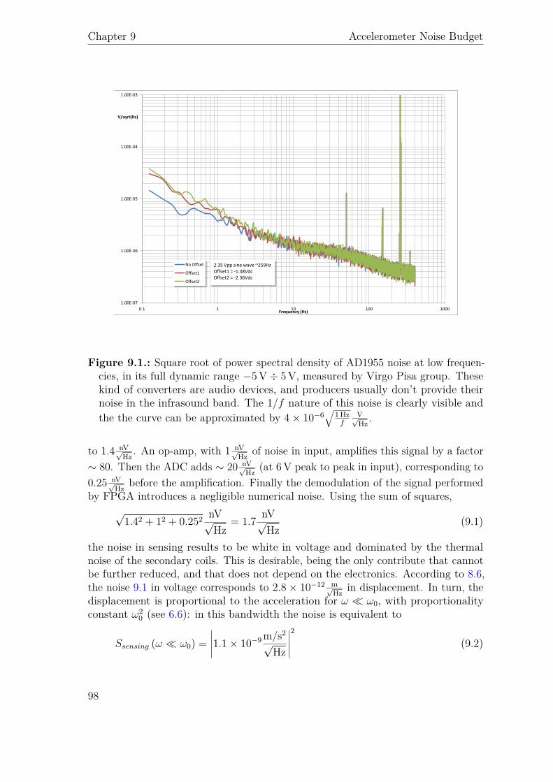
Chapter 9 Accelerometer Noise Budget

1.00E-07

1.00E-06

1.00E-05

1.00E-04

1.00E-03

0.1 1 10 100 1000

V/sqrt(Hz)

Frequency (Hz)

No Offset

Offset1

Offset2

2.35 Vpp sine wave ~259Hz Offset1 = -1.48Vdc Offset2 = -2.36Vdc

Figure 9.1.: Square root of power spectral density of AD1955 noise at low frequen-cies, in its full dynamic range −5V÷ 5V, measured by Virgo Pisa group. Thesekind of converters are audio devices, and producers usually don’t provide theirnoise in the infrasound band. The 1/f nature of this noise is clearly visible andthe the curve can be approximated by 4× 10−6

√1 Hzf

V√Hz .

to 1.4 nV√Hz . An op-amp, with 1 nV√

Hz of noise in input, amplifies this signal by a factor∼ 80. Then the ADC adds ∼ 20 nV√

Hz (at 6V peak to peak in input), corresponding to0.25 nV√

Hz before the amplification. Finally the demodulation of the signal performedby FPGA introduces a negligible numerical noise. Using the sum of squares,

√1.42 + 12 + 0.252 nV√

Hz= 1.7 nV√

Hz(9.1)

the noise in sensing results to be white in voltage and dominated by the thermalnoise of the secondary coils. This is desirable, being the only contribute that cannotbe further reduced, and that does not depend on the electronics. According to 8.6,the noise 9.1 in voltage corresponds to 2.8× 10−12 m√

Hz in displacement. In turn, thedisplacement is proportional to the acceleration for ω ω0, with proportionalityconstant ω2

0 (see 6.6): in this bandwidth the noise is equivalent to

Ssensing (ω ω0) =∣∣∣∣∣1.1× 10−9m/s2

√Hz

∣∣∣∣∣2

(9.2)

98

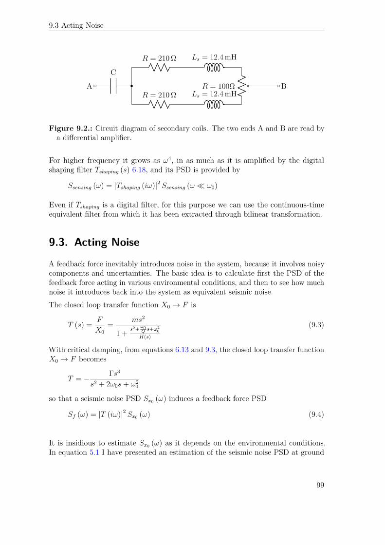
9.3 Acting Noise

A

C

R = 210 Ω Ls = 12.4mH

R = 100ΩR = 210 Ω Ls = 12.4mH

B

Figure 9.2.: Circuit diagram of secondary coils. The two ends A and B are read bya differential amplifier.

For higher frequency it grows as ω4, in as much as it is amplified by the digitalshaping filter Tshaping (s) 6.18, and its PSD is provided by

Ssensing (ω) = |Tshaping (iω)|2 Ssensing (ω ω0)

Even if Tshaping is a digital filter, for this purpose we can use the continuous-timeequivalent filter from which it has been extracted through bilinear transformation.

9.3. Acting Noise

A feedback force inevitably introduces noise in the system, because it involves noisycomponents and uncertainties. The basic idea is to calculate first the PSD of thefeedback force acting in various environmental conditions, and then to see how muchnoise it introduces back into the system as equivalent seismic noise.The closed loop transfer function X0 → F is

T (s) = F

X0= ms2

1 + s2+ ω0Qs+ω2

0H(s)

(9.3)

With critical damping, from equations 6.13 and 9.3, the closed loop transfer functionX0 → F becomes

T = − Γs3

s2 + 2ω0s+ ω20

so that a seismic noise PSD Sx0 (ω) induces a feedback force PSD

Sf (ω) = |T (iω)|2 Sx0 (ω) (9.4)

It is insidious to estimate Sx0 (ω) as it depends on the environmental conditions.In equation 5.1 I have presented an estimation of the seismic noise PSD at ground

99

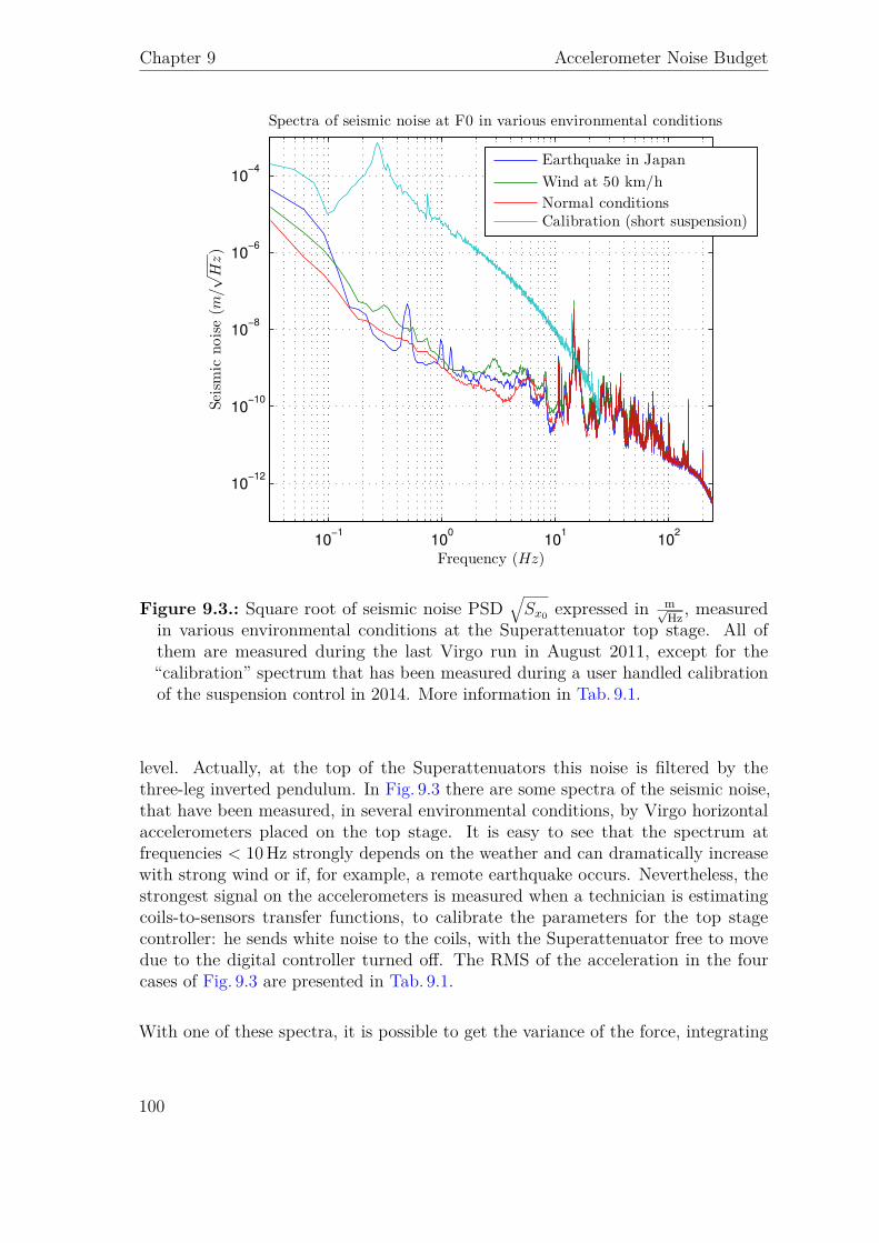
Chapter 9 Accelerometer Noise Budget

10−1

100

101

102

10−12

10−10

10−8

10−6

10−4

Spectra of seismic noise at F0 in various environmental conditions

Frequency (Hz)

Seism

icnoise(m

/√

Hz)

Earthquake in Japan

Wind at 50 km/h

Normal conditionsCalibration (short suspension)

Figure 9.3.: Square root of seismic noise PSD√Sx0 expressed in m√

Hz , measuredin various environmental conditions at the Superattenuator top stage. All ofthem are measured during the last Virgo run in August 2011, except for the“calibration” spectrum that has been measured during a user handled calibrationof the suspension control in 2014. More information in Tab. 9.1.

level. Actually, at the top of the Superattenuators this noise is filtered by thethree-leg inverted pendulum. In Fig. 9.3 there are some spectra of the seismic noise,that have been measured, in several environmental conditions, by Virgo horizontalaccelerometers placed on the top stage. It is easy to see that the spectrum atfrequencies < 10Hz strongly depends on the weather and can dramatically increasewith strong wind or if, for example, a remote earthquake occurs. Nevertheless, thestrongest signal on the accelerometers is measured when a technician is estimatingcoils-to-sensors transfer functions, to calibrate the parameters for the top stagecontroller: he sends white noise to the coils, with the Superattenuator free to movedue to the digital controller turned off. The RMS of the acceleration in the fourcases of Fig. 9.3 are presented in Tab. 9.1.

With one of these spectra, it is possible to get the variance of the force, integrating

100

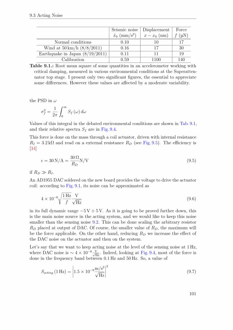
9.3 Acting Noise

Seismic noise Displacement Forcex0 (mm/s2) x− x0 (nm) f (µN)

Normal conditions 0.10 10 17Wind at 50 km/h (8/8/2011) 0.16 17 30

Earthquake in Japan (8/19/2011) 0.11 11 19Calibration 0.59 1100 140

Table 9.1.: Root mean square of some quantities in an accelerometer working withcritical damping, measured in various environmental conditions at the Superatten-uator top stage. I present only two significant figures, the essential to appreciatesome differences. However these values are affected by a moderate variability.

the PSD in ω

σ2f = 1

2π

ˆ ∞0

Sf (ω) dω

Values of this integral in the debated environmental conditions are shown in Tab. 9.1,and their relative spectra Sf are in Fig. 9.4.This force is done on the mass through a coil actuator, driven with internal resistanceRI = 3.2 kΩ and read on a external resistance RD (see Fig. 9.5). The efficiency is[34]

ε = 30N/A = 30 ΩRD

N/V (9.5)

if RD RI .An AD1955 DAC soldered on the new board provides the voltage to drive the actuatorcoil: according to Fig. 9.1, its noise can be approximated as

4× 10−6√

1Hzf

V√Hz

(9.6)

in its full dynamic range −5V÷ 5V. As it is going to be proved further down, thisis the main noise source in the acting system, and we would like to keep this noisesmaller than the sensing noise 9.2. This can be done scaling the arbitrary resistorRD placed at output of DAC. Of course, the smaller value of RD, the maximum willbe the force applicable. On the other hand, reducing RD we increase the effect ofthe DAC noise on the actuator and then on the system.Let’s say that we want to keep acting noise at the level of the sensing noise at 1Hz,where DAC noise is ∼ 4× 10−6 V√

Hz . Indeed, looking at Fig. 9.4, most of the force isdone in the frequency band between 0.1Hz and 50Hz. So, a value of

Sacting (1Hz) =∣∣∣∣∣1.5× 10−9m/s2

√Hz

∣∣∣∣∣2

(9.7)

101

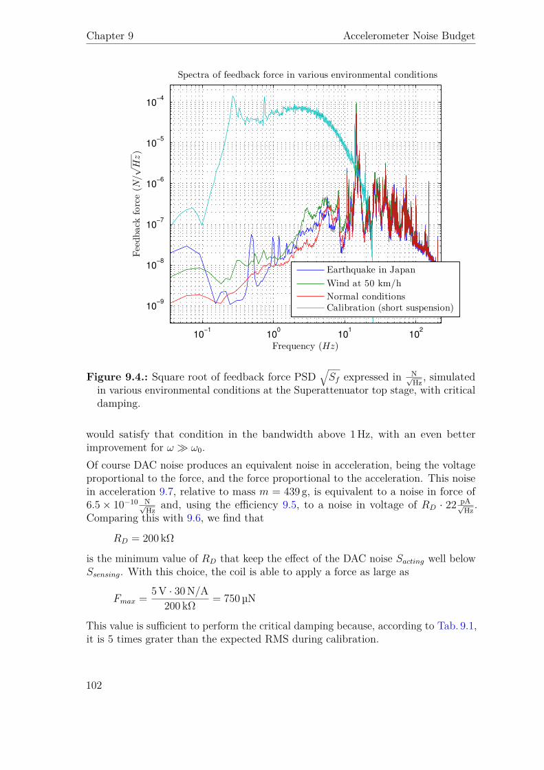
Chapter 9 Accelerometer Noise Budget

10−1

100

101

102

10−9

10−8

10−7

10−6

10−5

10−4

Spectra of feedback force in various environmental conditions

Frequency (Hz)

Feedback

force(N

/√

Hz)

Earthquake in Japan

Wind at 50 km/h

Normal conditionsCalibration (short suspension)

Figure 9.4.: Square root of feedback force PSD√Sf expressed in N√

Hz , simulatedin various environmental conditions at the Superattenuator top stage, with criticaldamping.

would satisfy that condition in the bandwidth above 1Hz, with an even betterimprovement for ω ω0.Of course DAC noise produces an equivalent noise in acceleration, being the voltageproportional to the force, and the force proportional to the acceleration. This noisein acceleration 9.7, relative to mass m = 439 g, is equivalent to a noise in force of6.5× 10−10 N√

Hz and, using the efficiency 9.5, to a noise in voltage of RD · 22 pA√Hz .

Comparing this with 9.6, we find that

RD = 200 kΩ

is the minimum value of RD that keep the effect of the DAC noise Sacting well belowSsensing. With this choice, the coil is able to apply a force as large as

Fmax = 5V · 30N/A200 kΩ = 750 µN

This value is sufficient to perform the critical damping because, according to Tab. 9.1,it is 5 times grater than the expected RMS during calibration.

102

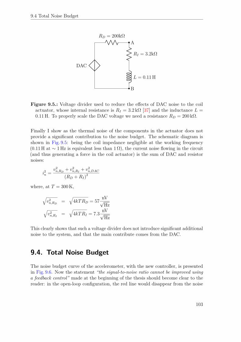
9.4 Total Noise Budget

DAC

RD = 200kΩA

RI = 3.2kΩ

L = 0.11H

B

Figure 9.5.: Voltage divider used to reduce the effects of DAC noise to the coilactuator, whose internal resistance is RI = 3.2 kΩ [37] and the inductance L =0.11H. To properly scale the DAC voltage we need a resistance RD = 200 kΩ.

Finally I show as the thermal noise of the components in the actuator does notprovide a significant contribution to the noise budget. The schematic diagram isshown in Fig. 9.5: being the coil impedance negligible at the working frequency(0.11H at ∼ 1Hz is equivalent less than 1 Ω), the current noise flowing in the circuit(and thus generating a force in the coil actuator) is the sum of DAC and resistornoises:

i2n =v2n,RD

+ v2n,RI

+ v2n,DAC

(RD +RI)2

where, at T = 300K,

√v2n,RD

=√

4kTRD = 57 nV√Hz√

v2n,RI

=√

4kTRI = 7.3 nV√Hz

This clearly shows that such a voltage divider does not introduce significant additionalnoise to the system, and that the main contribute comes from the DAC.

9.4. Total Noise Budget

The noise budget curve of the accelerometer, with the new controller, is presentedin Fig. 9.6. Now the statement “the signal-to-noise ratio cannot be improved usinga feedback control” made at the beginning of the thesis should become clear to thereader: in the open-loop configuration, the red line would disappear from the noise

103

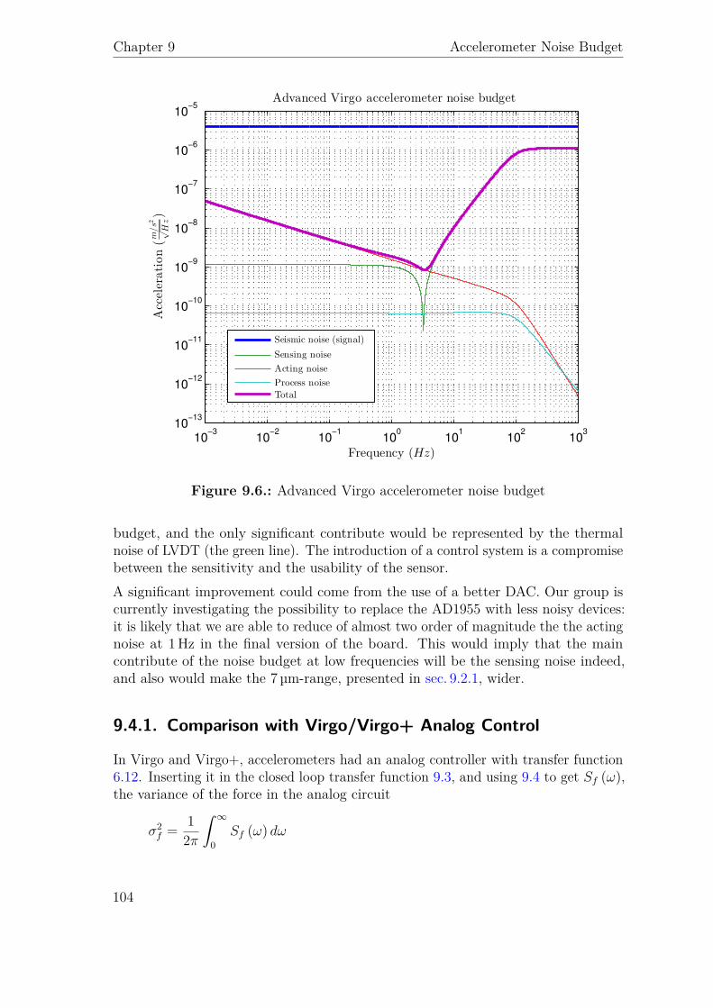
Chapter 9 Accelerometer Noise Budget

10−3

10−2

10−1

100

101

102

103

10−13

10−12

10−11

10−10

10−9

10−8

10−7

10−6

10−5

Advanced Virgo accelerometer noise budget

Frequency (Hz)

Acceleration(m/s2

√

Hz)

Seismic noise (signal)

Sensing noise

Acting noise

Process noise

Total

Figure 9.6.: Advanced Virgo accelerometer noise budget

budget, and the only significant contribute would be represented by the thermalnoise of LVDT (the green line). The introduction of a control system is a compromisebetween the sensitivity and the usability of the sensor.A significant improvement could come from the use of a better DAC. Our group iscurrently investigating the possibility to replace the AD1955 with less noisy devices:it is likely that we are able to reduce of almost two order of magnitude the the actingnoise at 1Hz in the final version of the board. This would imply that the maincontribute of the noise budget at low frequencies will be the sensing noise indeed,and also would make the 7 µm-range, presented in sec. 9.2.1, wider.

9.4.1. Comparison with Virgo/Virgo+ Analog Control

In Virgo and Virgo+, accelerometers had an analog controller with transfer function6.12. Inserting it in the closed loop transfer function 9.3, and using 9.4 to get Sf (ω),the variance of the force in the analog circuit

σ2f = 1

2π

ˆ ∞0

Sf (ω) dω

104

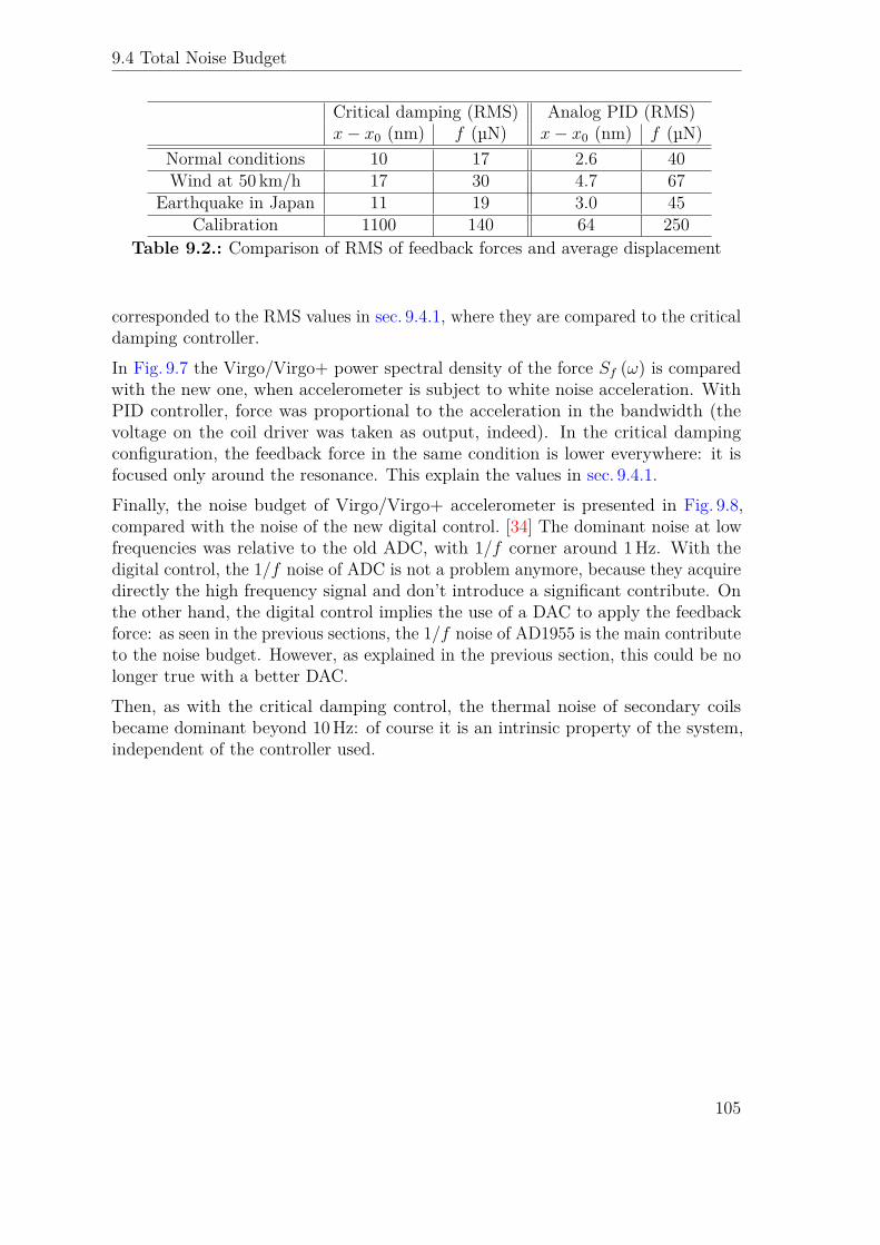
9.4 Total Noise Budget

Critical damping (RMS) Analog PID (RMS)x− x0 (nm) f (µN) x− x0 (nm) f (µN)

Normal conditions 10 17 2.6 40Wind at 50 km/h 17 30 4.7 67

Earthquake in Japan 11 19 3.0 45Calibration 1100 140 64 250

Table 9.2.: Comparison of RMS of feedback forces and average displacement

corresponded to the RMS values in sec. 9.4.1, where they are compared to the criticaldamping controller.In Fig. 9.7 the Virgo/Virgo+ power spectral density of the force Sf (ω) is comparedwith the new one, when accelerometer is subject to white noise acceleration. WithPID controller, force was proportional to the acceleration in the bandwidth (thevoltage on the coil driver was taken as output, indeed). In the critical dampingconfiguration, the feedback force in the same condition is lower everywhere: it isfocused only around the resonance. This explain the values in sec. 9.4.1.Finally, the noise budget of Virgo/Virgo+ accelerometer is presented in Fig. 9.8,compared with the noise of the new digital control. [34] The dominant noise at lowfrequencies was relative to the old ADC, with 1/f corner around 1Hz. With thedigital control, the 1/f noise of ADC is not a problem anymore, because they acquiredirectly the high frequency signal and don’t introduce a significant contribute. Onthe other hand, the digital control implies the use of a DAC to apply the feedbackforce: as seen in the previous sections, the 1/f noise of AD1955 is the main contributeto the noise budget. However, as explained in the previous section, this could be nolonger true with a better DAC.Then, as with the critical damping control, the thermal noise of secondary coilsbecame dominant beyond 10Hz: of course it is an intrinsic property of the system,independent of the controller used.

105

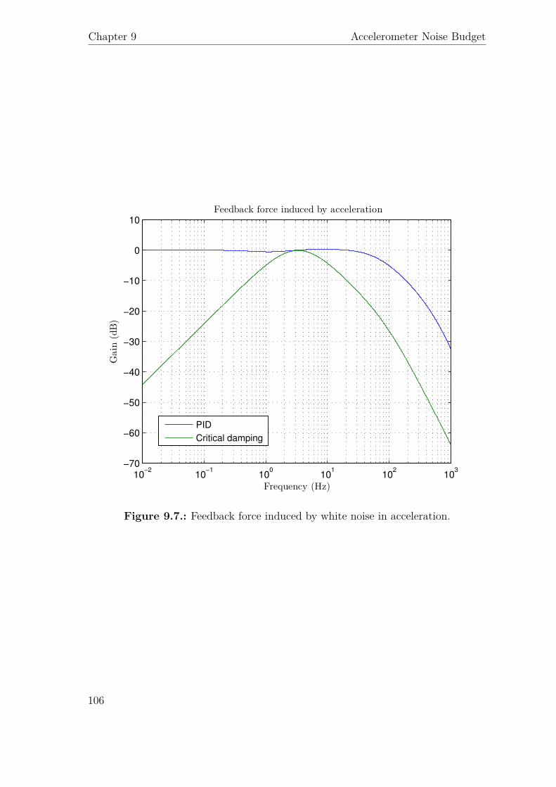
Chapter 9 Accelerometer Noise Budget

10−2

10−1

100

101

102

103

−70

−60

−50

−40

−30

−20

−10

0

10Feedback force induced by acceleration

Frequency (Hz)

Gain

(dB)

PID

Critical damping

Figure 9.7.: Feedback force induced by white noise in acceleration.

106

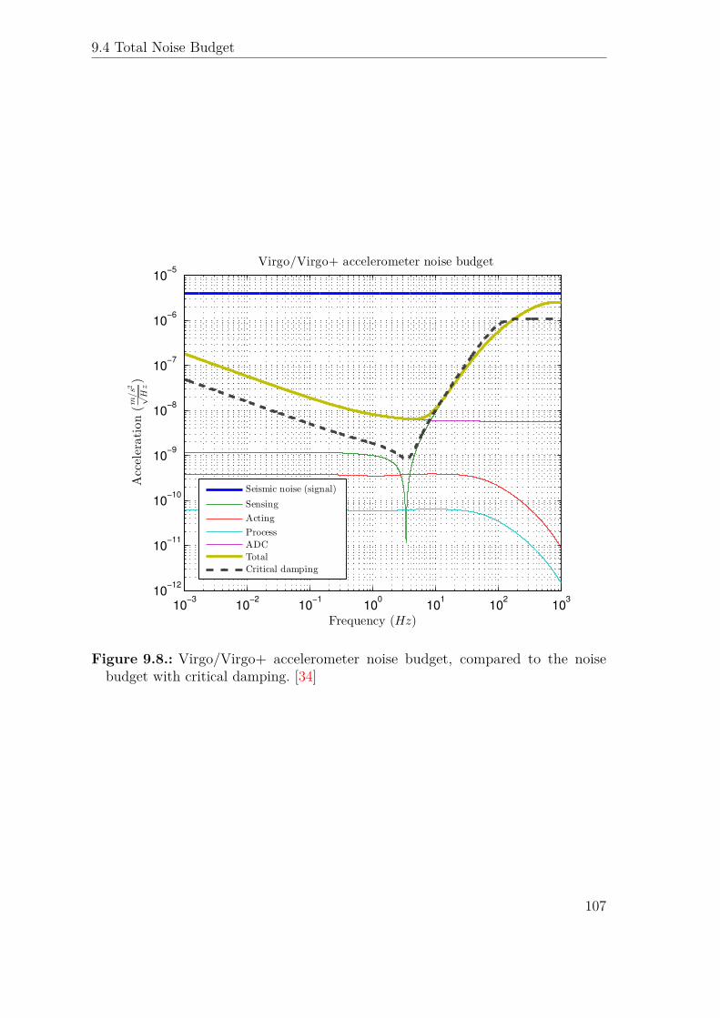
9.4 Total Noise Budget

10−3

10−2

10−1

100

101

102

103

10−12

10−11

10−10

10−9

10−8

10−7

10−6

10−5

Virgo/Virgo+ accelerometer noise budget

Frequency (Hz)

Acceleration(m/s2

√

Hz)

Seismic noise (signal)

Sensing

Acting

Process

ADC

Total

Critical damping

Figure 9.8.: Virgo/Virgo+ accelerometer noise budget, compared to the noisebudget with critical damping. [34]

107

10Conclusions

It is less than two years from the beginning of the data acquisition, and the projectAdvanced Virgo is going to make operative the interferometer with a never beforeachieved sensitivity. To be ready to detect gravitational signals from many potentialsources around our galaxy, every single part of Virgo is undergoing several upgrades.In this thesis I have presented a description as exhaustive as possible of horizontalaccelerometers, currently used over the Superattenuators to measure the seismicnoise. While the mechanics of the sensor will remain the same, the electronicsthat controls accelerometers is completely rebuilt. In particular, a dedicated board,hosting their analog controller in Virgo, disappears: the DSP of the new electronicsof the Superattenuator inertial control is enough powerful to take care also of thecontrol of accelerometers.I have designed a digital control system for the horizontal accelerometers. It makespossible to reduce by a factor 2 the external force applied to the pendulum forthe feedback control, with respect to the old controller used in Virgo and Virgo+.This, together with the better performances of the new ADC and DAC, lets usto increase of almost one order of magnitude the sensitivity of the sensors in thefrequency band from DC to 3Hz. Furthermore, this improvement could be evenlarger if current digital-to-analog converters are replaced with better ones. Becauseof the great importance of such a thing, our group is currently investigating thispossibility. In the future, the critical damping control have to be extended for verticalaccelerometers.Using the noise levels of the new components, I have also defined a limit to thedynamic range of the position of the pendulum inside the accelerometer: with thecurrent DAC, it must be kept within ∼ 7 µm from the center, in order to limit theeffects of the noise on primary coil of LVDT over the accelerometer sensitivity. Ofcourse, this range would be wider using a better DAC.Eventually, I have created an algorithm to synthesize sinusoidal waves with a DDS,and then to demodulate the signal from secondary coils of LVDT. Using a digital

109

Chapter 10 Conclusions

closed loop system, this algorithm measures the phase shift between reference waveand signal, and then adjusts itself in order to get the best signal-to-noise ratiofrom LVDT. This algorithm, implemented in FPGA, can be used not only foraccelerometers, but of course also for the others LVDTs used in Superattenuatorinertial control.Furthermore, a purely digital control applied to accelerometers brings about a lotof other advantages. For example, the DDS realized with the FPGA let us to dowithout the commercial signal generators, that have been used so far in Virgo, onefor each Superattenuator, to drive LVDT inside the accelerometers. In addition toan obvious savings opportunity relative to their maintenance, we can also suppose tosend signals at slightly different frequencies to the various LVDT, in order to avoidpossible electromagnetic interferences that could arise between sensors.In conclusion, the potentialities of the new electronics are enormous. Besides theinertial control of Superattenuators, the computational resources of DSP and FPGAare sufficient to host many new features, compared to what it was in Virgo andVirgo+.

110

AMathematical Tools

A.1. Laplace Transform

Laplace transform is a linear operator of a function f (t) with a real argument t(t ≥ 0) that transforms f (t) to a function F (s) with complex argument s, given bythe integral

L [f (t)] (s) = F (s) =ˆ ∞

0+f (τ) e−sτdτ (A.1)

This transformation is bijective for the majority of practical uses.

A.1.1. Inverse Laplace Transform

The inverse Laplace transform is

L−1 [F (s)] (t) = 12πi lim

T→∞

ˆ γ+iT

γ−iTF (s)estds, (A.2)

where the integration is done along the vertical line Re(s) = γ in the complex planesuch that γ is greater than the real part of all singularities of F (s).

The set of values for which F (s) converges is known as the region of convergence.

A.1.2. Used Properties

Table of the used properties:

111

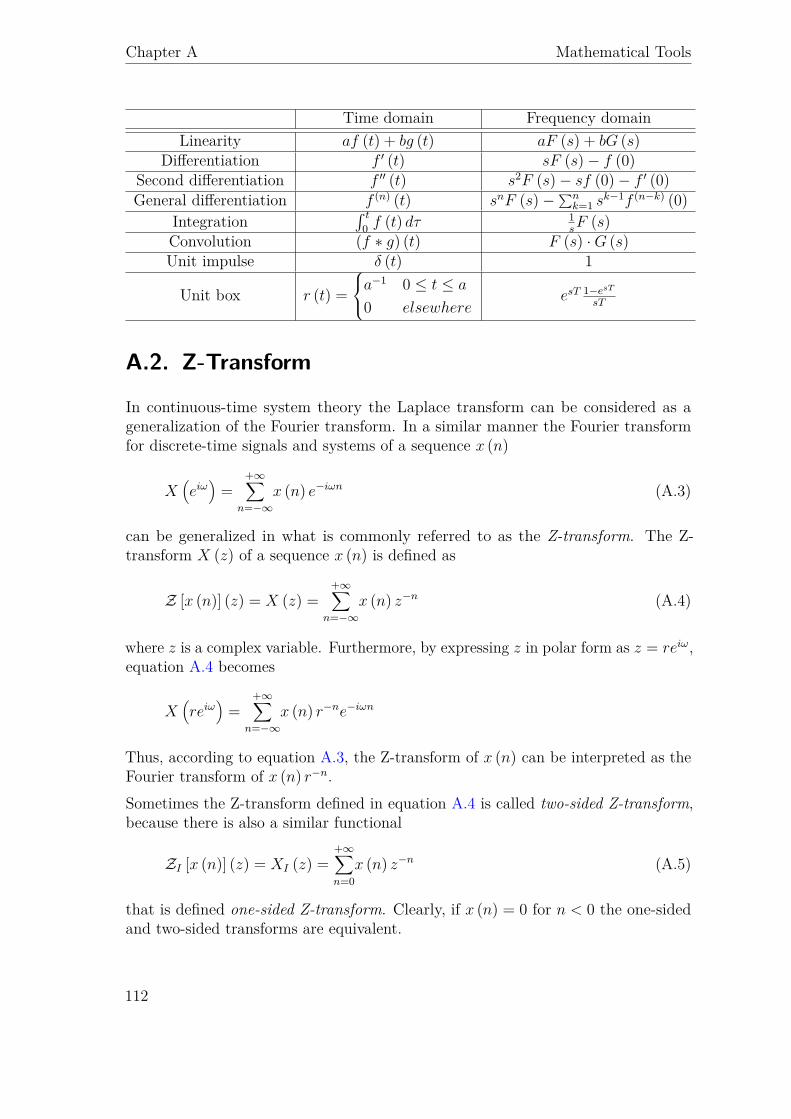
Chapter A Mathematical Tools

Time domain Frequency domainLinearity af (t) + bg (t) aF (s) + bG (s)

Differentiation f ′ (t) sF (s)− f (0)Second differentiation f ′′ (t) s2F (s)− sf (0)− f ′ (0)General differentiation f (n) (t) snF (s)−∑n

k=1 sk−1f (n−k) (0)

Integration´ t

0 f (t) dτ 1sF (s)

Convolution (f ∗ g) (t) F (s) ·G (s)Unit impulse δ (t) 1

Unit box r (t) =a−1 0 ≤ t ≤ a

0 elsewhereesT 1−esT

sT

A.2. Z-Transform

In continuous-time system theory the Laplace transform can be considered as ageneralization of the Fourier transform. In a similar manner the Fourier transformfor discrete-time signals and systems of a sequence x (n)

X(eiω)

=+∞∑

n=−∞x (n) e−iωn (A.3)

can be generalized in what is commonly referred to as the Z-transform. The Z-transform X (z) of a sequence x (n) is defined as

Z [x (n)] (z) = X (z) =+∞∑

n=−∞x (n) z−n (A.4)

where z is a complex variable. Furthermore, by expressing z in polar form as z = reiω,equation A.4 becomes

X(reiω

)=

+∞∑n=−∞

x (n) r−ne−iωn

Thus, according to equation A.3, the Z-transform of x (n) can be interpreted as theFourier transform of x (n) r−n.Sometimes the Z-transform defined in equation A.4 is called two-sided Z-transform,because there is also a similar functional

ZI [x (n)] (z) = XI (z) =+∞∑n=0

x (n) z−n (A.5)

that is defined one-sided Z-transform. Clearly, if x (n) = 0 for n < 0 the one-sidedand two-sided transforms are equivalent.

112

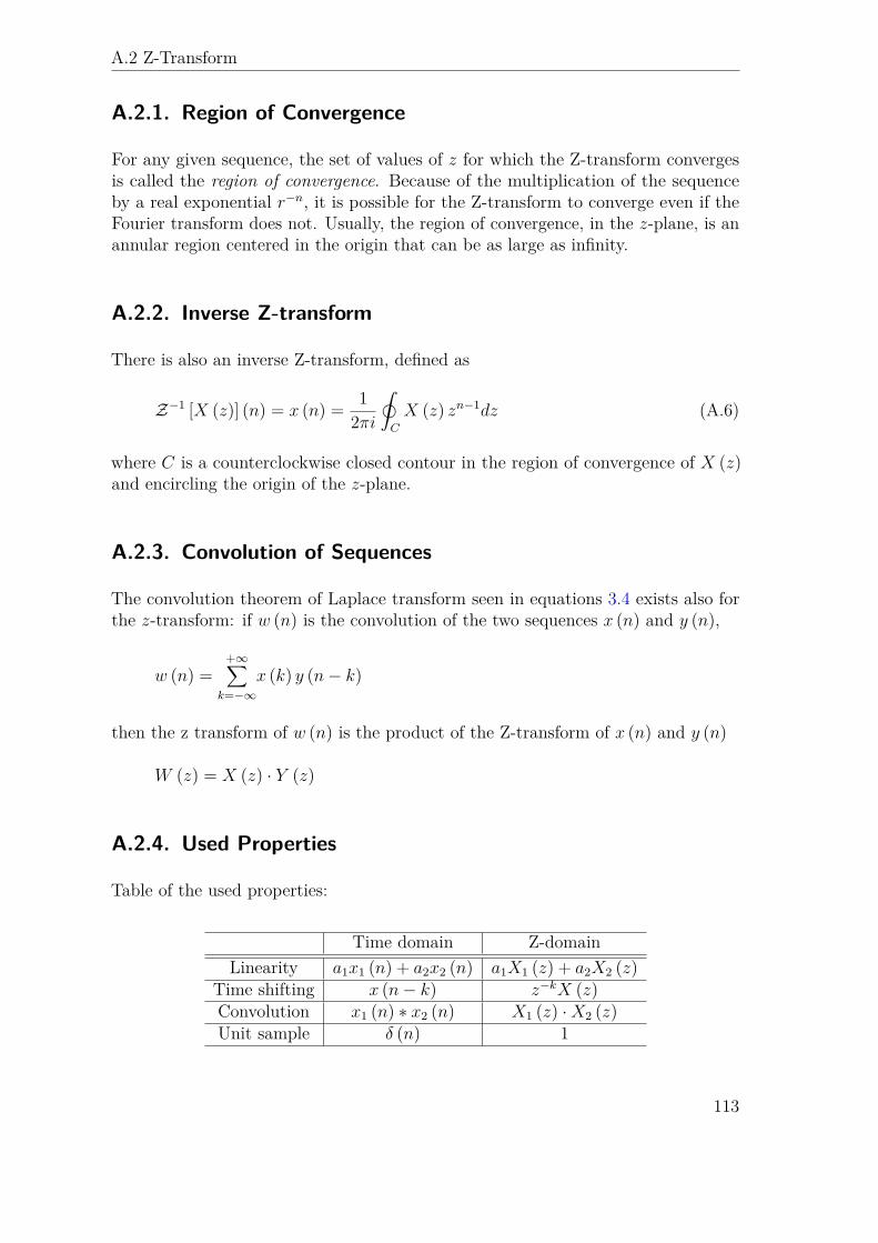
A.2 Z-Transform

A.2.1. Region of Convergence

For any given sequence, the set of values of z for which the Z-transform convergesis called the region of convergence. Because of the multiplication of the sequenceby a real exponential r−n, it is possible for the Z-transform to converge even if theFourier transform does not. Usually, the region of convergence, in the z-plane, is anannular region centered in the origin that can be as large as infinity.

A.2.2. Inverse Z-transform

There is also an inverse Z-transform, defined as

Z−1 [X (z)] (n) = x (n) = 12πi

˛C

X (z) zn−1dz (A.6)

where C is a counterclockwise closed contour in the region of convergence of X (z)and encircling the origin of the z-plane.

A.2.3. Convolution of Sequences

The convolution theorem of Laplace transform seen in equations 3.4 exists also forthe z-transform: if w (n) is the convolution of the two sequences x (n) and y (n),

w (n) =+∞∑

k=−∞x (k) y (n− k)

then the z transform of w (n) is the product of the Z-transform of x (n) and y (n)

W (z) = X (z) · Y (z)

A.2.4. Used Properties

Table of the used properties:

Time domain Z-domainLinearity a1x1 (n) + a2x2 (n) a1X1 (z) + a2X2 (z)

Time shifting x (n− k) z−kX (z)Convolution x1 (n) ∗ x2 (n) X1 (z) ·X2 (z)Unit sample δ (n) 1

113

Chapter A Mathematical Tools

A.3. Bilinear Transformation

Suppose we have the following first order differential equation

a1y′(t) + a0y(t) = b0x(t) (A.7)

where, obviously, y′(t) is the time derivative of y(t). Using a Laplace transform andassuming as initial condition y(0+) = 0 we get

a1sY (s) + a0Y (S) = b0X(s)

from which we obtain the transfer function

Ha(s) = Y (s)X(s) = b0

a1s+ a0(A.8)

Obviously we have

y(t) =ˆ t

t0

y′(τ)dτ + y(t0)

and, putting t = nT and t0 = (n−1)T in this last equation (f = 1/T is the samplingfrequency), we get:

y(nT ) =ˆ nT

(n−1)Ty′(τ)dτ + y((n− 1)T )

Approximating the integral by the trapezoidal rule we obtain:

y(nT ) ' y((n− 1)T ) + T

2 [y′(nT ) + y′((n− 1)T )] (A.9)

On the other hand we have from eq. A.7

y′(nT ) = −a0

a1y(nT ) + b0

a1x(nT )

putting this last equation into eq. A.9 we get

yn − yn−1 'T

2

[−a0

a1(yn + yn−1) + b0

a1(xn + xn−1)

]

where we’ve written yn instead of y(nT ). Now, using the Z-transform and remem-bering that if xn → X(z) then xn−1 → z−1X(z), we obtain:

H(z) = Y (z)X(z) = b0

a12T

1−z−1

1+z−1 s+ a0(A.10)

114

A.3 Bilinear Transformation

Comparing the analog transfer function A.8 with the discrete one in A.10, we seethat we can obtain the latter from the former simply by substituting the s Laplace’svariable with the following expression:

s→ 2T

1− z−1

1 + z−1 (A.11)

Obviously we can obtain an analog transfer function from a discrete one using theinverse transformation:

z → 1 + T/2 s1− T/2 s (A.12)

The transformation A.11 is called bilinear transformation. We obtain it in thecase of a first order linear differential equation. Nevertheless its validity is moregeneral, because an N th-order linear differential equation can be written as a set ofN first order linear differential equations.

115

BTechnical Tools

B.1. Mechanical Impedances

In the electrical world, the impedance is the measure of the opposition that a circuitpresents to a current when a voltage is applied, ans is represented as a complexquantity Ze. Is defined as the complex ratio of the Laplace transforms of the voltageV to the current I:

Ze = V

I(B.1)

Under the assumption that all initial conditions are zero, the characteristic differentialequation of a series RLC circuit with applied an external voltage V is

LsI +RI + C−1 1sI = V (B.2)

Similarly, the characteristic differential equation of a forced damped harmonicoscillator with null initial conditions is

ms2X + γsX + kX = F (B.3)

It’s easy to see that these two systems can be studied with the same mathematicaltools if we associate the physical quantities as shown in table B.1.It follows that we can define a mechanical impedance Zm as the ratio of the externalforce F to the velocity of the system v = sX:

Zm = F

v(B.4)

This is a measure of how much a structure resists motion when subjected to a givenforce, and has the dimension of a damping coefficient. It’s interesting to observe thatthe the product of V and I, elements of equation X is dimensioned as a power, so asthat of F and v.

117

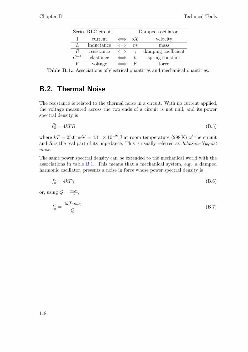
Chapter B Technical Tools

Series RLC circuit Damped oscillatorI current ⇐⇒ sX velocityL inductance ⇐⇒ m massR resistance ⇐⇒ γ damping coefficientC−1 elastance ⇐⇒ k spring constantV voltage ⇐⇒ F force

Table B.1.: Associations of electrical quantities and mechanical quantities.

B.2. Thermal Noise

The resistance is related to the thermal noise in a circuit. With no current applied,the voltage measured across the two ends of a circuit is not null, and its powerspectral density is

v2n = 4kTR (B.5)

where kT = 25.6meV = 4.11× 10−21 J at room temperature (298K) of the circuitand R is the real part of its impedance. This is usually referred as Johnson–Nyquistnoise.The same power spectral density can be extended to the mechanical world with theassociations in table B.1. This means that a mechanical system, e.g. a dampedharmonic oscillator, presents a noise in force whose power spectral density is

f 2n = 4kTγ (B.6)

or, using Q = mω0γ

,

f 2n = 4kTmω0

Q(B.7)

118

CNotes on Seismic Noise

C.1. An Analytic Approach

Instead of using the measured values of seismic noise, we can use the spectrum 5.1,that allows a parametric solution:

Sx0 (f) ∼∣∣∣∣∣∣A ·

(1Hzf

)2 m√Hz

∣∣∣∣∣∣2

(where A = 10−7). According to 9.4, this induce, in the critical damped system, afeedback force with power spectral density of

Sf (ω) = |T (iω)|2 Sx0 (ω)This becomes

Sf (ω) =∣∣∣∣∣− Γ (iω)3

(iω)2 + 2ω0 (iω) + ω20

∣∣∣∣∣2 (4π2A

ω2

)2

=(

4π2ΓAωω2 + ω2

0

)2

With one of these spectra, it’s possible to get the variance of the force, integratingthe PSD in ω

σ2f = 1

2π

ˆ ∞0

Sf (ω) dω

= 12π

ˆ ∞0

(4π2ΓAωω2 + ω2

0

)2

dω

= (4π2ΓA)2

2π

ˆ ∞0

ω2

(ω2 + ω20)2dω

= (4π2ΓA)2

2ππ

4ω0= 2π4Γ2A2

ω0

119

Chapter C Notes on Seismic Noise

Using the right values, this corresponds to a standard deviation

σf = 40 µN

that is consistent with estimations presented in Tab. 9.1.

120

Bibliography

[1] J. Abadie et al., “Predictions for the Rates of Compact Binary CoalescencesObservable by Ground-based Gravitational-wave Detectors,” Class.Quant.Grav.,vol. 27, p. 173001, 2010.

[2] The Virgo Collaboration, “Advanced Virgo Technical Design Report,” Tech.Rep. VIR–0128A–12, CNRS and INFN, Apr 2012.

[3] J. Beringer et al., “Review of Particle Physics,” Phys.Rev., vol. D86, p. 010001,2012.

[4] I. R. Kenyon, General Relativity. Oxford University Press, 1990.

[5] S. Weinberg, Gravitation and cosmplogy: principles and applications of thegeneral theory of relativity. John Wiley & Sons, Inc., 1972.

[6] R. Feynman, R. Leighton, and M. Sands, The Feynman Lectures on Physics -Mainly Electromagnetism and Matter. Addison-Wesley Publishing Company,Inc., 1964.

[7] J. Weisberg, D. Nice, and J. Taylor, “Timing Measurements of the RelativisticBinary Pulsar PSR B1913+16,” Astrophys.J., vol. 722, pp. 1030–1034, 2010.

[8] P. Peters and J. Mathews, “Gravitational radiation from point masses in aKeplerian orbit,” Phys.Rev., vol. 131, pp. 435–439, 1963.

[9] P. Ade et al., “BICEP2 I: Detection Of B-mode Polarization at Degree AngularScales,” 2014.

[10] K. S. Thorne, Gravitational Radiation in "Three Hundred Years of Gravitation".Cambridge University Press, 1987.

[11] The LIGO Scientific Collaboration, “http://www.ligo.org/science/gw-sources.php,” 2014.

121

Bibliography

[12] C. D. Ott, E. Abdikamalov, P. Mösta, R. Haas, S. Drasco, et al., “General-Relativistic Simulations of Three-Dimensional Core-Collapse Supernovae,” As-trophys.J., vol. 768, p. 115, 2013.

[13] J. Abadie et al., “Search for gravitational waves associated with gamma-raybursts during LIGO science run 6 and Virgo science runs 2 and 3,” Astrophys.J.,vol. 760, p. 12, 2012.

[14] J. Aasi, J. Abadie, B. Abbott, R. Abbott, T. Abbott, et al., “Gravitationalwaves from known pulsars: results from the initial detector era,” 2013.

[15] B. Allen, “The stochastic gravity-wave background: sources and detection,” inRelativistic Gravitation and Gravitational Radiation, Proceedings of the LesHouches School of Physics, held in Les Houches, Haute Savoie, vol. 26, pp. 373–418, 1997.

[16] T. Regimbau, “The astrophysical gravitational wave stochastic background,”Res.Astron.Astrophys., vol. 11, pp. 369–390, 2011.

[17] B. Abbott et al., “An Upper Limit on the Stochastic Gravitational-Wave Back-ground of Cosmological Origin,” Nature, vol. 460, p. 990, 2009.

[18] G. Diambrini-Palazzi, “Gravitational radiation produced by high-energy acceler-ators and high power lasers,” Part.Accel., vol. 33, pp. 195–205, 1990.

[19] P. Saulson, Fundamentals of Interferometric Gravitational Wave Detectors.World Scientific Publishing Company, Incorporated, 1994.

[20] The AURIGA collaboration, “AURIGA website,” May 2009.

[21] V. Boschi, Modeling and Simulation of Seismic Attenuation Systems for Gravi-tational Wave Interferometers. PhD thesis, Università di Pisa, 2010.

[22] K. Ogata, Modern Control Engineering. Instrumentation and controls series,Prentice Hall, 2010.

[23] J. Maciejowski, Multivariable feedback design. Electronic systems engineeringseries, Addison-Wesley, 1989.

[24] A. V. Oppenheim and R. Schafer, Digital signal processing. Prentice-Hallinternational editions, Prentice-Hall, 1975.

[25] M. Punturo, “Advanced Virgo sensitivity curve study.” VIR-0073D-12, Nov2012.

[26] R. Del Fabbro, “Magnetic antispring.” VIR-NOT-PIS-1380-71, Dec 1993.

[27] SAT group, “Strategy for adv superattenuators.” VIR-0098A-08, October 2008.

[28] A. Gennai, “Technical Requirements For a HRG Sensor Prototype.” VIR-0661B-11, Sep 2012.

[29] V. Boschi, “Gyroscope Characterization Study.” VIR-0032B-14, Feb 2014.

122

Bibliography

[30] Texas Instruments, TMS320C6678 - Multicore Fixed and Floating-Point Dig-ital Signal Processor (Rev. E). Texas Instruments, SPRS691E—November2010—Revised March 2014 ed., Mar 2014.

[31] G. Losurdo, G. Calamai, E. Cuoco, L. Fabbroni, G. Guidi, M. Mazzoni,R. Stanga, F. Vetrano, L. Holloway, D. Passuello, et al., “Inertial controlof the mirror suspensions of the VIRGO interferometer for gravitational wavedetection,” Review of Scientific Instruments, vol. 72, no. 9, pp. 3653–3661, 2001.

[32] T. Zelenova, “Horizontal Accelerometer.” VIR-0775A-09, 2009.[33] Bruel & Kjaer, LAN-XI Data Acquisition Hardware for PULSETM and Test for

I-deasTM. Bruel & Kjaer, bp 2215 – 15 ed., 08 2009.[34] M. Passuello, “Accelerometer Noise Budget.” 2009.[35] R. Poley, “Signal Conditioning an LVDT Using a TMS320F2812 DSP,” Appli-

cation Report SPRA946, Texas Instruments, August 2003.[36] M. Kumm, “DDS Synthesizer,” 2008.[37] N. Grilli, “Measurements on Accelerometers Coils.” VIR-0061A-12, 02 2012.

123

Nomenclature

ADC Analog-to-Digital converter

AdV Advanced Virgo

BBN Big Bang Nucleosynthesis

CMB Cosmic Microwave Background

DAC Digital-to-Analog converter

DSP Digital Signal Processor

F0 Filter 0

F7 Filter 7

FIFO First In, First Out

FPGA Field Programmable Gate Array

GR General Relativity

HRG Hemispherical Resonator Gyroscope

ID Inertial Damping

IP Inverted Pendulum

LQG Linear-Quadratic-Gaussian

LTI Linear Time-Invariant system

LUT Look-Up Table

125

Nomenclature

LVDT Linear Variable Differential Transformer

MIMO Multiple-Input and Multiple-Output

NCO Numerically Controlled Oscillator

PA Phase Accumulator

PAC Phase-to-Amplitude Converter

PID Proportional-Integral-Derivative controller

PLL Phase-Locked Loop

PSD Power Spectral Density

SA Superattenuator

SF Standard Filter

SGWB Stochastic Gravitational-Wave Background

SISO Single-Input and Single-Output

SNR Signal-to-Noise Ratio

SR Special Theory of Relativity

126