Embed Size (px)
Citation preview

Templates and Recurrences: Better TogetherJason Breck
[email protected] of Wisconsin
Madison, WI, USA
John [email protected]
University of WisconsinMadison, WI, USA
Zachary [email protected]
Princeton UniversityPrinceton, NJ, USA
Thomas [email protected]
University of WisconsinMadison, WI, USA
AbstractThis paper is the confluence of two streams of ideas in theliterature on generating numerical invariants, namely: (1)template-based methods, and (2) recurrence-based methods.
A template-based method begins with a template that con-tains unknown quantities, and finds invariants that matchthe template by extracting and solving constraints on theunknowns. A disadvantage of template-based methods isthat they require fixing the set of terms that may appear inan invariant in advance. This disadvantage is particularlyprominent for non-linear invariant generation, because theuser must supply maximum degrees on polynomials, basesfor exponents, etc.On the other hand, recurrence-based methods are able to
find sophisticated non-linear mathematical relations, includ-ing polynomials, exponentials, and logarithms, because suchrelations arise as the solutions to recurrences. However, adisadvantage of past recurrence-based invariant-generationmethods is that they are primarily loop-based analyses: theyuse recurrences to relate the pre-state and post-state of aloop, so it is not obvious how to apply them to a recursiveprocedure, especially if the procedure is non-linearly recur-sive (e.g., a tree-traversal algorithm).In this paper, we combine these two approaches and ob-
tain a technique that uses templates in which the unknownsare functions rather than numbers, and the constraints on theunknowns are recurrences. The technique synthesizes invari-ants involving polynomials, exponentials, and logarithms,even in the presence of arbitrary control-flow, including anycombination of loops, branches, and (possibly non-linear)recursion. For instance, it is able to show that (i) the timetaken by merge-sort isO(n log(n)), and (ii) the time taken byStrassen’s algorithm is O(nlog2(7)).
This paper is an extended version of a paper with the sametitle at PLDI 2020 [5].
CCS Concepts: • Software and its engineering→ Auto-mated static analysis; • Theory of computation→ Pro-gram analysis.
Keywords: Invariant generation, Recurrence relation
1 IntroductionA large body of work within the numerical-invariant-generation literature focuses on template-based methods[10, 31]. Such methods fix the form of the invariants thatcan be discovered, by specifying a template that containsunknown quantities. Given a program and some propertyto be proved, a template-based analyzer proceeds by findingconstraints on the values of the unknowns and then solvingthese constraints to obtain invariants of the program thatsuffice to prove the property. Template-based methods havebeen particularly successful for finding invariants within thedomain of linear arithmetic.
Many programs have important numerical invariants thatinvolve non-linear mathematical relationships, such as poly-nomials, exponentials, and logarithms. A disadvantage oftemplate-based methods for non-linear invariant generationis that (in contrast to the linear case) there is no “most gen-eral” template term, so the user must supply the set of termsthat may appear in the invariant.
In this paper, we present an invariant-synthesis techniquethat is related to template-based methods, but sidesteps theabove difficulty. Our technique is based on a concept that wecall a hypothetical summary, which is a template for a proce-dure summary in which the unknowns are functions, ratherthan numbers. The constraints that we extract for these func-tions are recurrences. Solving these recurrence constraintsallows us to synthesize terms over program variables thatwe can substitute in place of the unknown functions in ourtemplate and thereby obtain procedure summaries.
Whereas most template-based methods directly constrainthe mathematical form of their invariants, our techniqueconstrains the invariants indirectly, by way of recurrences,and thereby allows the invariants to have a wide variety ofmathematical forms involving polynomials, exponentials,and logarithms. This aspect is intuitively illustrated by therecurrences S(n) = 2S(n/2) + n and T (n) = 2T (n/2) + n2:although these two recurrences are outwardly similar, theirsolutions are more different than one would expect at firstglance, in that S(n) is Θ(n logn), whereas T (n) is Θ(n2). Be-cause the unknowns in our templates are functions, we can
arX
iv:2
003.
1351
5v1
[cs
.PL
] 3
0 M
ar 2
020

Jason Breck, John Cyphert, Zachary Kincaid, and Thomas Reps
generate a wide variety of invariants (involving polynomi-als, exponentials, logarithms) without specifying their exactsyntactic form.However, recurrence-based invariant-generation tech-
niques typically have disadvantages when applied to recur-sive programs. Recurrences are well-suited to characterizethe sequence of states that occur as a loop executes. Thisidea can be extended to handle linear recursion—where arecursive procedure makes only a single recursive call: eachprocedure-entry state that occurs “on the way down” to thebase case of the recursion is paired with the correspondingprocedure-exit state that occurs “on the way back up” fromthe base case, and then recurrences are used to describe thesequence of such state pairs. However, non-linear recursionhas a different structure: it is tree-shaped, rather than linear,and thus some kind of additional abstraction is required be-fore non-linear recursion can be described using recurrences.
We use the technique of hypothetical summaries to extendthe work of [14], [25], and [24]: hypothetical summaries en-able a different approach to the analysis of non-linearly recur-sive programs, such as divide-and-conquer or tree-traversalalgorithms.1 We show how to analyze the base case of aprocedure to extract a template for a procedure summary(i.e., a hypothetical summary). By assuming that every callto the procedure, throughout the tree of recursive calls, isconsistent with the template, we discover relationships (i.e.,recurrence constraints) among the states of the program atdifferent heights in the tree. We then solve the constraintsand fill in the template to obtain a procedure summary. Hy-pothetical summaries thus provide the additional layer ofabstraction that is required to apply recurrence-based invari-ant generation to non-linearly recursive procedures.Our invariant generation procedure is both (1) general-
purpose, so it is applicable to a wide variety of tasks, and(2) compositional, so the space and time required to analyzea program fragment depends on the size of the fragmentrather than the whole program. In contrast, conventionaltemplate-based methods are goal-directed (they must be tai-lored to a specific problem of interest, e.g., a template-basedinvariant generator for verification problems cannot solvequantitative problems such as resource-bound analysis) andwhole-program. The general-purpose nature of our proce-dure also distinguishes it from recurrence-based resource-bound analyses, which for example cannot be applied toassertion checking.
1Warning: We use the term “non-linear” in two different senses: non-linearrecursion and non-linear arithmetic. Even for a loop that uses linear arith-metic, non-linear arithmetic may be required to state a loop invariant.Moreover, arithmetic expressions in the programs that we analyze are notlimited to linear arithmetic: variables can be multiplied.The two uses of the term “non-linear” are essentially unrelated, and
which term is intended should be clear from context. The paper primarilyconcerns new techniques for handling non-linear recursion, and non-lineararithmetic is handled by known methods, e.g., [25].
To evaluate the applicability of our analysis to challengingnumerical-invariant-synthesis tasks, we applied it to the taskof generating bounds on the computational complexity ofnon-linearly recursive programs and the task of generatinginvariants that suffice to prove assertions. Our experimentsshow that the analysis technique is able to prove propertiesthat [24] was not capable of proving, and is competitivewith the output of state-of-the-art assertion-checking andresource-bound-analysis tools.
Contributions. Our work makes contributions in threemain areas:1. We introduce an analysis method based on “hypothetical
summaries.” It hypothesizes that a summary exists of aparticular form, using uninterpreted function symbols tostand for unknown expressions. Analysis is performedto obtain constraints on the function symbols, which arethen solved to obtain a summary.
2. We develop a procedure-summarization technique calledheight-based recurrence analysis, which uses the notion ofhypothetical summaries to produce bounds on the valuesof program variables based on the height of recursion(§4.1). We further develop algorithms that, when used inconjunction with height-based recurrence analysis (§4.2and §4.3), yield more precise summaries. Furthermore,we give an algorithm (§4.4) that generalizes height-basedrecurrence analysis to the setting of mutual recursion.
3. The technique is implemented in the CHORA tool. Our ex-periments show that CHORA is able to handle many non-linearly recursive programs, and generate invariants thatinclude exponentials, polynomials, and logarithms (§5).For instance, it is able to show that (i) the time taken bymerge-sort isO(n log(n)), (ii) the time taken by Strassen’salgorithm is O(nlog2(7)), and (iii) an iterative function anda non-linearly recursive function that both perform expo-nentiation are functionally equivalent.
§2 presents an example to provide intuition. §3 provides back-ground on material needed for understanding the paper’sresults. §6 discusses related work.
2 OverviewThe goal of this paper is to find numerical summaries forall the procedures in a given program. For simplicity, thissection discusses the analysis of a program that contains asingle procedure P , which is non-linearly recursive and callsno other procedures.
We use the following example to illustrate how our tech-niques use recurrence solving to summarize non-linearly-recursive procedures.
Example 2.1. The function subsetSum (Fig. 1) takes an ar-ray A of n integers, and performs a brute-force search todetermine whether any non-empty subset of A’s elementssums to zero. If it finds such a set, it returns the number of

Templates and Recurrences: Better Together
int nTicks; bool f ound ;int subsetSum(int ∗A, int n) {
found = false; return subsetSumAux(A, 0,n, 0);}int subsetSumAux(int ∗A, int i, int n, int sum) {
nTicks++;if (i >= n) {
if (sum == 0) { found = true; }return 0;
}int size = subsetSumAux(A, i + 1,n, sum +A[i]);if (found) { return size + 1; }size = subsetSumAux(A, i + 1,n, sum);return size;
}
1rec. call
Time
nTicks′ - nTicks - 1 ≤ b2(h+1)
2
height h+1pre-state
3
nTicks′ - nTicks - 1 ≤ b2(h) nTicks′ - nTicks - 1 ≤ b2(h)
rec. call4 5 6
height ≤ hpre-state
height ≤ h post-state
height h+1post-state
height ≤ hpre-state
height ≤ h post-state
Figure 1. Example program subsetSum. The diagram at the bottomshows a timeline of a height (h + 1) execution of subsetSumAux.b2(h + 1) is related to the increase of nTicks between the pre-state(label 1) and the post-state (label 6). b2(h) is related to the increaseof nTicks between (2) and (3) and also between (4) and (5), i.e.,between the pre-states and post-states of height-h executions.
elements in the set, and otherwise it returns zero. The recur-sive function subsetSumAux works by sweeping through thearray from left to right, making two recursive calls for eacharray element. The first call considers subsets that includethe element A[i], and the second call considers subsets thatexclude A[i]. The sum of the values in each subset is com-puted in the accumulating parameter sum. When the basecase is reached, subsetSumAux checks whether sum is zero,and if so, sets found to true. At each of the two recursivecall sites, the value returned by the recursive call is stored inthe variable size. After found is set to true, subsetSumAuxcomputes the size of the subset by returning size + 1 if thesubset was found after the first recursive call, or returningsize unchanged if the subset was found after the secondrecursive call.In this paper, a state of a program is an assignment of
integers to program variables. For each procedure P , we wishto characterize the relational semantics R(P), defined as theset of state pairs (σ ,σ ′) such that P can start executing instate σ and finish in state σ ′. To find an over-approximate
representation of the relational semantics of a recursive pro-cedure such as subsetSumAux, we take an approach that wecall height-based recurrence analysis. In height-based recur-rence analysis, we construct and solve recurrence relationsto discover properties of the transition relation of a recursiveprocedure. To formalize our use of recurrence relations, wegive the following definitions.
We define the height-bounded relational semantics R(P ,h)to be the subset of R(P) that P can achieve if it is limited tousing an execution stack with a height of at mosth activationrecords. We define a height-h execution of P to be any exe-cution of P that uses a stack height of at most h, or, in otherwords, an execution of P having recursion depth no morethan h. Base cases are defined to be of height 1. Let τ1, ...,τnbe a set of polynomials over unprimed and primed programvariables, representing the pre-state and post-state of P , re-spectively. For each τk we associate a function Vk : N→ 2Q,such that Vk (h) is defined to be the set of values v such that,for some (σ ,σ ′) ∈ R(P ,h), τk evaluates tov by using σ and σ ′to interpret the unprimed and primed variables, respectively.Using subsetSumAux as an example, let τ1
def= return′.
Then, V1(1) denotes the set of values return′ can take onin any base case of subsetSumAux. In this program, return′is 0 in any base case, and so V1(1) = {0}. Now consideran execution of height 2. In the case that found is true, wehave that return′ increases by 1 compared to the valuethat return′ has in the base case. If found is not true thenreturn′ remains the same. In other words, at height-2 execu-tions, return′ takes on the values 0 and 1; i.e.,V1(2) = {0, 1}.Similarly, V1(3) = {0, 1, 2}, and so on. We approximate thevalue set Vk (h) by finding a function bk (h) : N → Q thatbounds Vk (h) for all h; that is, for any v ∈ Vk (h), we havev ≤ bk (h). In the case of τ1, a suitable bounding functionb1(h) is b1(h) = h− 1. The initial step of our analysis choosesterms τ1, ...,τn , and then for each term τk , tries to synthesizea function bk (h) that bounds the set of values τk can take on.Note that for a given term τj , a corresponding bounding
function may not exist. A necessary condition for a bound-ing function to exist for a term τj is that the set Vj (1) mustbe bounded. This observation restricts our set of candidateterms τ1, ...,τn to only be over terms that are bounded abovein the base case. (Specifically, we require the expressions tobe bounded above by zero.) For example, return′ ≤ 0 in thebase case, and so τ1
def= return′ is a candidate term. Similarly,
the term τ2def= nTicks’-nTicks-1 is also bounded above by
0 in the base case, and so τ2 is a candidate term. There areother candidate terms that our analysis would extract for thisexample, but for brevity they are not listed here. We discoverthese bounded terms τ1 and τ2 using symbolic abstraction(see §3).
Once we have a set of candidate terms τ1, ...,τn , we seek tofind corresponding bounding functions b1(h), ...,bk (h). Notethat such functions may not exist: just because τk is bounded
Jason Breck, John Cyphert, Zachary Kincaid, and Thomas Reps
above in the base case does not mean it is bounded in allother executions. If a bounding function for a term does exist,we would like a closed-form expression for it in terms of h.We derive such closed-form expressions by hypothesizingthat a bounding functionbk (h) does exist. These hypotheticalfunctionsbk (h) allow us to construct a hypothetical proceduresummary φh that represents a typical height-h execution. Forexample, in the case of subsetSumAux:
φhdef= return′ ≤ b1(h) ∧ nTicks′ − nTicks − 1 ≤ b2(h).
Note that, although φh assumes the existence of severalbounding functions (corresponding to bk (h) for several val-ues of k), the assumptions for different values of k need notall succeed or fail together. That is, if we fail to find a bound-ing function bk (h) for some k , this failure does not preventus from continuing the analysis and finding other boundingfunctions (bj (h), with j , k) for the same procedure.
We then build up a height-(h + 1) summary, φh+1, compo-sitionally, with φh replacing the recursive calls. For example,consider the term τ2 = nTicks′−nTicks−1 in the context ofFig. 1. Our goal is to create a relational summary for the vari-able nTicks between labels 1 and 6. We do this by extendinga summary for the transition between labels 1 and 2 witha summary for the transition between 2 and 3, namely, ourhypothetical summary. Then we extend that with a summaryfor the paths between labels 3 and 4, and so on. Betweenlabels 1 and 2, nTicks gets increased by 1. We then summa-rize the transition between 1 and 3. We know nTicks getsincreased by 1 between labels 1 and 2. Furthermore, our hy-pothetical bounding function nTicks′ − nTicks − 1 ≤ b2(h)says that nTicks gets increased by at most b2(h)+1 betweenlabels 2 and 3. Combining these summaries, we see thatnTicks gets increased by at most b2(h) + 2 between labels1 and 3. nTicks does not change between labels 3 and 4,so the summary between labels 1 and 4 is the same as theone between labels 1 and 3. The transition between labels4 and 5 is a recursive call, so we again use our hypotheticalsummary to approximate this transition. Once again, sucha summary says nTicks gets increased by at most b2(h) + 1.Extending our summary for the transition between 1 and4 with this information allows us to conclude that nTicksgets increased by at most 2b2(h) + 3 between labels 1 and5. nTicks does not change between labels 5 and 6. Conse-quently, our summary for nTicks between labels 1 and 6is nTicks′ − nTicks ≤ 2b2(h) + 3. Similar reasoning wouldalso obtain a summary for return as return′ ≤ 1 + b1(h).These formulas constitute our height-(h + 1) hypotheticalsummary, φh+1.
φh+1def= return′ ≤ 1+b1(h) ∧ nTicks′ ≤ nTicks+2b2(h)+3
If we rearrange each conjunct to respectively place τ1 and τ2on the left-hand-side of each inequality, we obtain height-(h + 1) bounds on the values of τ1 and τ2. By definition such
bounds are valid expressions for b1(h+ 1) and b2(h+ 1). Thatis at height-(h + 1),
return′ ≤ b1(h) + 1 = b1(h + 1) (1)nTicks′ − nTicks − 1 ≤ 2 + 2b2(h) = b2(h + 1) (2)
The equations give recursive definitions forb1 andb2. Solvingthese recurrence relations give us bounds on the value setsV1(h) and V2(h), for all heights h.
In §4.2, we present an algorithm that determines an upperbound on a procedure’s depth of recursion as a function ofthe parameters to the initial call and the values of globalvariables. This depth of recursion can also be interpretedas a stack height h that we can use as an argument to thebounding functions bk (h). In the case of subsetSumAux, weobtain the bound h ≤ max(1, 1 + n − i). The solutions to therecurrences discussed above, when combined with the depthbound, yield the following summary.
nTicks′ ≤ nTicks + 2h − 1 ∧ return′ ≤ h − 1 ∧h ≤ max(1, 1 + n − i)
When subsetSum is called with some array size n, the max-imum possible depth of recursion that can be reached bysubsetSumAux is equal to n. In this way, we have establishedthat the running time of subsetSum is exponential in n, andthe return value is at most n.
3 BackgroundRelational semantics. In the following, we give an ab-
stract presentation of the relational semantics of programs.Fix a set Var of program variables. A state σ : State def
=
Var → Z consist of an integer valuation for each programvariable. A recursive procedure P can be understood as achain-continuous (and hence monotonic) function on staterelations F JPK : 2State×State → 2State×State . The relationalsemantics RJPK of P is given as the limit of the ascendingKleene chain of F JPK:
R(P , 0) = ∅R(P ,h + 1) = F JPK(R(P ,h))
RJPK =⋃h∈N
R(P ,h)
Operationally, for anyhwemay viewR(P ,h) as the input/out-put relation of P on a machine with a stack limit of h acti-vation records. We can extend relational semantics to mutu-ally recursive procedures in the natural way, by consideringF JPK to be function that takes as input a k-tuple of staterelations (where k is the number of mutually recursive pro-cedures).A transition formula φ is a formula over the program
variables Var and an additional set Var ′ of “primed” copies,representing the values of the program variables before andafter a computation. A transition relation φ can be inter-preted as a property that holds of a pair of states (σ ,σ ′): we
Templates and Recurrences: Better Together
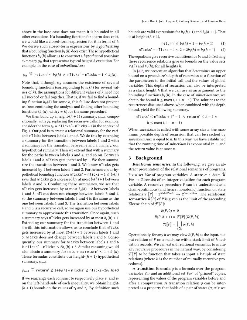
Algorithm 1: The convex-hull algorithm from [14]Input :Formula of the form ∃X .ψ whereψ is satisfiable and
quantifier-freeOutput :Convex hull of ∃X .ψ
1 P ← ⊥;2 while there exists a modelm ofψ do3 Let Q be a cube of the DNF ofψ s.t.m |= Q ;4 Q ← project(Q,X ) ; /* Polyhedral projection */
5 P ← P ⊔Q ; /* Polyhedral join */
6 ψ ← ψ ∧ ¬P ;7 return P
say that (σ ,σ ′) satisfies φ if φ is true when each variablein Var is interpreted according to σ , and each variable inVar ′ is interpreted according to σ ′. We use RJφK to denotethe state relation consisting of all pairs (σ ,σ ′) that satisfyφ. This paper is concerned with the problem of proceduresummarization, in which the goal is to find a transition for-mula φ that over-approximates a procedure, in the sense thatRJPK ⊆ RJφK.
A relational expressionτ is a polynomial overVar∪Var ′with rational coefficients. A relational expression can be eval-uated at a state pair (σ ,σ ′) ∈ State × State by using σ to in-terpret the unprimed symbols and σ ′ to interpret the primedsymbols—we use EJτ K(σ ,σ ′) to denote the evaluation of τat (σ ,σ ′).
Intra-procedural analysis. The technique for proce-dure summarization developed in this paper makes useof intra-procedural summarization as a sub-routine. Weformalize this intra-procedural technique by a functionPathSummary(e,x ,V ,E), which takes as input a control-flow graph with vertices V , edges E, entry vertex e , andexit vertex x , and computes a transition formula that over-approximates all paths in (V ,E) between e and x . We useSummary(P ,φ) to denote a function that takes as input arecursive procedure P and a transition formula φ, and com-putes a transition formula that over-approximates P whenφ is used to interpret recursive calls (i.e., F JPK(RJφK) ⊆RJSummary(P ,φ)K). Summary(P ,φ) can be implemented interms of PathSummary(e,x ,V ,E) by replacing all call edgeswith φ, and taking (e,x ,V ,E) to be the control-flow graphof P .In principle, any intra-procedural summarization proce-
dure can be used to implement Summary(P ,φ); the imple-mentation of our method uses the technique from Kincaidet al. [25].
Symbolic abstraction. We useAbstract(φ,V ) to denote aprocedure that takes a formula φ and computes a set of poly-nomial inequations over the variables V that are implied byφ. If φ is expressed in linear arithmetic, then a representationof all implied polynomial inequations (namely, a constraintrepresentation of the convex hull of φ projected onto V ) canbe computed effectively (e.g., using [14, Alg. 2], which we
show in this paper as Alg. 1). Otherwise, we settle for a soundprocedure that produces inequations implied by φ, but notnecessarily all of them (e.g., using [25, Alg. 3]).
In principle, the convex hull of a linear arithmetic formulaF can be computed as follows: write F in disjunctive normalform, as F ≡ C1 ∨ ... ∨Cn , where eachCi is a conjunction oflinear inequations (i.e., a convex polyhedron). The convexhull of F is obtained by replacing disjunctions with the joinoperator of the domain of convex polyhedra. This algorithmcan be improved by using an SMT solver to enumerate theDNF lazily, and extended to handle existential quantificationby using polyhedral projection (Alg. 1). A similar approachcan be used to compute a conjunction of non-linear inequa-tions that are implied by a formula F , by treating non-linearterms in the formula as additional dimensions of the space(e.g., a quadratic inequation x2 < y2 is treated as a linearinequation dx 2 < dy2 , where dx 2 and dy2 are symbols thatwe associate with the terms x2 and y2, but have no intrin-sic meaning). The non-linear variation of the algorithm’sprecision can be improved by using inference rules, congru-ence closure, and Grobner-basis algorithms to deduce linearrelations among the non-linear dimensions that are conse-quences of the non-linear theory ([25, Alg. 3]). Note that,because non-linear integer arithmetic is undecidable, thisprocess is (necessarily) incomplete.
Recurrence relations. C-finite sequences are a well-studied class of sequences defined by linear recurrence rela-tions, of which a famous example is the Fibonacci sequence.Formally,
Definition 3.1. A sequence s : N→ Q is C-finite of orderd if it satisfies a linear recurrence equation
s(k + d) = c1s(k + d − 1) + ... + cd−1s(k + 1) + cds(k) ,where each ci is a constant.
It is classically known that every C-finite sequence s(k)admits a closed form that is computable from its recurrencerelation and takes the form of an exponential-polynomial
s(k) = p1(k)rk1 + p2(k)rk2 + ... + pl (k)rkl ,where each pi is a polynomial in k and each ri is a constant.In the following, it will be convenient to use a different kindof recurrence relation to present C-finite sequences, namelystratified systems of polynomial recurrences.
Definition 3.2. A stratified system of polynomial recur-rences is a system of recurrence equations over sequencesx1,1, ...,x1,n1 , ...,xm,1, ...,xm,nm of the form{xi, j (k + 1) = ci, j,1xi,1(k) +· · · + ci, j,nixi,ni (k) + pi, j }i, j
where each ci, j,1, ..., ci, j,ni is a constant, and pi, j is a polyno-mial in x1,1(k), ...,x1,n1 (k), ...,xi−1,1(k), ...,xi−1,ni−1 (k).
Intuitively, the sequences x1,1, ...,x1,n1 , ...,xm,1, ...,xm,nmare organized into strata (x1,1, ...,x1,n1 is the first,

Jason Breck, John Cyphert, Zachary Kincaid, and Thomas Reps
x2,1, ...,x2,n1 is the second, and so on), the right-hand-sideof the equation for xi, j can involve linear terms over thesequences in the i th strata, and additional polynomial termsover sequences of lower strata. It follows from the closureproperties of C-finite sequences that each xi, j defines aC-finite sequence, and an exponential-polynomial closedform for each sequence can be computed from a stratifiedsystem of polynomial recurrences [22]. The fact that anyC-finite sequence satisfies a stratified system of polynomialrecurrences follows from the fact that a recurrence of orderd can be implemented as a system of linear recurrencesamong d sequences [22].
Example 3.3. An example of a stratified system of polyno-mial recurrences with four sequences (w,x ,y, z) arrangedinto two strata ((w,x) and (y, z)) is as follows:[
w(k + 1)x(k + 1)
]=
[1 1
30 2
] [w(k)x(k)
]+
[10
][y(k + 1)z(k + 1)
]=
[1 01 1
] [y(k)z(k)
]+
[x(k)2 + 1
3w(k) + x(k)
]This system has the closed-form solution
w(k) = w(0) + (2k − 1)3 x(0) + k x(k) = 2kx(0)
y(k) = 4k − 13 x(0)2 + y(0) + k
z(k) = 3w(0) + 4k − 3k − 19 x(0)2+
(2k+1 − k − 1)x(0) + ky(0) + z(0) + 2(k2 − k) .
4 Technical DetailsThis section gives algorithms for summarizing recursive pro-cedures using recurrence solving. We assume that beforethese algorithms are applied to the procedures of a programP, we first compute and collapse the strongly connectedcomponents of the call graph of P and topologically sort thecollapsed graph. Our analysis then works on the stronglyconnected components of the call graph in a single pass,in a topological order of the collapsed graph, by applyingthe algorithms of this section to recursive components, andapplying intraprocedural analysis to non-recursive compo-nents.For simplicity, §4.1 focuses on the analysis of strongly
connected components consisting of a single recursive pro-cedure P . The first step of the analysis is to apply Alg. 2,which produces a set of inequations that describe the valuesof variables in P . Not all of the inequations found by Alg. 2are suitable for use in a recurrence-based analysis, so weapply Alg. 3 to filter the set of inequations down to a subsetthat, when combined, form a stratified recurrence. The nextstep is to give this recurrence to a recurrence solver, whichresults in a logical formula relating the values of variablesin P to the stack height h that may be used by P . In §4.2, we
show how to (i) obtain a bound on h that depends on theprogram state before the initial call to P , and (ii) combinethe recurrence solution with that depth bound to create asummary of P . In §4.3, we discuss how to obtain a certainclass of more precise bounds (including lower bounds on therunning time of a procedure). In §4.4, we show how to ex-tend the techniques of §4.1 to handle programs with mutualrecursion, i.e., programs whose call graphs have stronglyconnected components consisting of multiple procedures. In§4.5, we discuss an extension of the algorithm of §4.4 thathandles sets of mutually recursive procedures in which someprocedures do not have base cases.
4.1 Height-Based Recurrence AnalysisLet τ be a relational expression and let P be a procedure. Weuse Vτ (P ,h) to denote the set of values of τ in a height-hexecution of P .
Vτ (P ,h)def= {EJτ K(σ ,σ ′) : (σ ,σ ′) ∈ R(P ,h)}
It consists of values to which τ may evaluate at a state pairbelonging to R(P ,h). We call bτ : N→ Q a bounding functionfor τ in P if for all h ∈ N and all v ∈ Vτ (P ,h), we havev ≤ bτ (h). Intuitively, the bounding function bτ (h) boundsthe value of an expression τ in any execution that uses stackheight at most h.
The goal of §4.1 is to find a set of relational expressions andassociated bounding functions. We proceed in three steps.First, we determine a set of candidate relational expressionsτ1, ...,τn . Second, we optimistically assume that there existfunctions b1(h), ...,bn(h) that bound these expressions, andwe analyze P under that assumption to obtain constraintsrelating the values of the relational expressions to the valuesof the b1(h), ...,bn(h) functions. Third, we re-arrange theconstraints into recurrence relations for each of the bk (h)functions (if possible) and solve them to synthesize a closed-form expression for bk (h) that is suitable to be used in asummary for P .
We begin our analysis of P by determining a set of suitableexpressions τ . If a relational expression τ has an associatedbounding function, then it must be the case thatVτ (P , 1) (i.e.,the set of values that τ takes on in the base case) is boundedabove. Without loss of generality, we choose expressions τ sothat Vτ (P , 1) is bounded above by zero. (Note that if Vτ (P , 1)is bounded above by c then Vτ−c (P , 1) is bounded above byzero.) We begin our analysis of P by analyzing the base caseto look for relational expressions that have this property.
Selecting candidate relational expressions. The rea-son for looking at expressions over program variables, asopposed to individual variables, is illustrated by Ex. 2.1: thevariable nTicks has a different value each time the base caseexecutes, but the expression nTicks′ − nTicks− 1 is alwaysequal to zero in the base case.

Templates and Recurrences: Better Together
Algorithm 2: Algorithm for extracting candidate recur-rence inequationsInput :A procedure P , and the associated vocabulary of
program variables VarOutput :Height-based-recurrence summary φheight
1 β ← Summary(P , false) ;2 wbase ← Abstract(β ,Var ∪ Var′) ;3 n ← the number of inequations inwbase;4 foreach k in 1, ...,n do5 Let τk be the expression over Var ∪ Var′ such that the kth
inequation inwbase is (τk ≤ 0) ;6 Let bk (·) be a fresh uninterpreted function symbol ;7 φcall ←
∧nk=1(τk ≤ bk (h) ∧ bk (h) ≥ 0) ;
8 φrec ← Summary(P ,φcall) ;9 φext ← φrec ∧
∧nk=1(bk (h + 1) = τk ) ;
10 S ← ∅;11 foreach k in 1, ...,n do12 wext,k ← Abstract(φext, {b1(h), ...,bn (h),bk (h + 1)}) ;13 foreach inequation I inwext,k do14 S ← S ∪ {I}15 return S
With the goal of identifying relational expressions thatare bounded above by zero, Alg. 2 begins by extracting atransition formula β for the non-recursive paths through Pby calling Summary(P , false) (i.e., summarizing P by usingfalse as a summary for the recursive calls in P ). Next, we com-pute a set wbase of polynomial inequations over Var ∪ Var′
(the set of un-primed (pre-state) and primed (post-state)copies of all global variables, along with unprimed copies ofthe parameters to P and the variable return′, which repre-sents the return value of P ) that are implied by β by callingAbstract(β ,Var ∪ Var′). Let n be the number of inequationsinwbase. Then, for k = 1, ...,n, we rewrite the kth inequationin the form τk ≤ 0. In the case of Ex. 2.1, τ1
def= return′ and
τ2def= nTicks′ − nTicks − 1 have the property that τ1 ≤ 0
and τ2 ≤ 0 in the base case.Note that there are, in general, many sets of relational
expressions τ1, ...,τn that are bounded above by zero in thebase case. The soundness of Alg. 2 only depends on Abstractchoosing some such set. Our implementation ofAbstract uses[25, Alg. 3], and is not guaranteed to choose the set of rela-tional expressions that would lead to the most precise resultsfor any given application, e.g., for a given assertion-checkingor complexity-analysis problem. Intuitively, in the case thatβ is a formula in linear arithmetic, our implementation ofAbstract amounts to using the operations of the polyhedralabstract domain to find a convex hull of β . Then, each ofthe inequations in the constraint representation of the con-vex hull can be interpreted as a relational expression that isbounded above by zero in the base case.
Generating constraints on bounding functions. Foreach of the expressions τk that has an upper bound in the
base case, we are ultimately looking to find a function bk (h)that is an upper bound on the value of that expression inany height-h execution. Our way of finding such a functionis to analyze the recursive cases of P to look for an invariantinequation that gives an upper bound on Vτk (P ,h + 1) interms of an upper bound on Vτk (P ,h). Such an inequationcan be interpreted as a recurrence relating bk (h + 1) to bk (h).
The remainder of Alg. 2 (Lines (7)–(14)) finds such invari-ant inequations. The first step is to create the hypotheticalprocedure summary φcall, which hypothesizes that a bound-ing function bτk exists for each expression τk , and that thevalue of that function at height h is an upper bound on thevalue of τk . φcall is a transition formula that represents aheight-h execution of P . In Ex. 2.1, φcall is:
return′ ≤ b1(h) ∧ nTicks′ − nTicks − 1 ≤ b2(h)∧b1(h) ≥ 0 ∧ b2(h) ≥ 0
On line (8), Alg. 2 calls Summary, using φcall as the rep-resentation of each recursive call in P , and the resultingtransition formula is stored in φrec. Thus, φrec describes atypical height-(h + 1) execution of P . In Ex. 2.1, a simplifiedversion of φrec is given as φh+1 in §2.
On line (9), the formula φext is produced by conjoiningφrec with a formula stating that, for each k , bk (h + 1) = τk .Therefore, φext implies that any upper bound on bk (h + 1)must be an upper bound on τk in any height-(h+1) execution.Ultimately, we wish to obtain a closed-form solution for
each bk (h). The formula φext implicitly determines a set ofrecurrences relating b1(h + 1), ...,bn(h + 1) to b1(h), ...,bn(h).However, φext does not have the explicit form of a recur-rence. Lines (12)–(14) abstract φext to a conjunction of in-equations that give an explicit relationship between bk (h+1)and b1(h), ...,bn(h) for each k .
Extracting and solving recurrences. The next step ofheight-based recurrence analysis is to identify a subset ofthe inequations returned by Alg. 2 that constitute a stratifiedsystem of polynomial recurrences (Defn. 3.2). This subsetmust meet the following three stratification criteria:1. Each bounding function bk (h + 1) must appear on the
left-hand-side of at most one inequation.2. If a bounding function bk (h) appears on the right-hand-
side of an inequation, then bk (h + 1) appears on someleft-hand-side.
3. It must be possible to organize the bk (h + 1) into strata,so that if bk (h) appears in a non-linear term on the right-hand-side of the inequation for bj (h + 1), then bk (h) mustbe on a strictly lower stratum than bk (h).Alg. 3 computes a maximal subset of inequations that
complies with the above three rules.The next step of height-based recurrence analysis is to
send this recurrence to a recurrence solver, such as the onedescribed in Kincaid et al. [25]. The solution to the recurrenceis a set of bounding functions. Let B be the set of indices k

Jason Breck, John Cyphert, Zachary Kincaid, and Thomas Reps
Algorithm 3: Algorithm for constructing a stratified re-currenceInput :A set of candidate inequations I1, ...,IN over the
function symbolsb1(h), ...,bn (h),b1(h + 1), ...,bn (h + 1)
Output :A set of inequations that form a stratified recurrence1 Let DefinesBound[j] be a map from integers to integers;2 Let UsesBound[j,k] and UsesBoundNonLinearly[j,k] be maps
that map all pairs of integers to false;3 S ← {1, ...,N } ;4 foreach j in 1, ...,N do5 Write Ij as bk (h + 1) ≤ c0 + Σ
mji=1ci (b1(h))
di,1 · · · (bn (h))di,nif Ij can be written in that form with 1 ≤ k ≤ n, ∀i . ci ∈ Q,∃i > 0. ci > 0, ∀i,p. di,p ∈ N; otherwise let S ← S − {j}and continue loop;
6 For i = 0, ...,mj , c ′i ← max(0, ci ) ;7 Let I ′j be bk (h + 1) ≤ c ′0 + Σ
mji=1c
′i (b1(h))
di,1 · · · (bn (h))di,n ;8 DefinesBound[j] := k ;9 foreach i ∈ {1, ..,mj } do
10 foreach p ∈ {1, ...,n} do11 if c ′i > 0 ∧ di,p > 0 then UsesBound[j,p] := true ;12 if c ′i > 0 ∧ di,p > 0 ∧ Σnq=1di,q > 1 then
UsesBoundNonLinearly[j,p] := true ;13 A← ∅ ;14 repeat15 V ← S −A;16 repeat17 foreach j ∈ V do18 if ∃k .UsesBound[j,k] ∧ ¬∃j ′ ∈ V .DefinesBound[j ′] = k
then V ← V − {j};19 if ∃k .UsesBoundNonLinearly[j,k] ∧ ¬∃j ′ ∈
A.DefinesBound[j ′] = k then V ← V − {j};20 until V is unchanged;21 foreach k = {1, ...,n} do22 if V contains more than one j such that
DefinesBound[j] = k then23 Arbitrarily choose one such j to remain in V , and
remove all other such j from V ;24 A← A ∪V ;25 until V = ∅;26 return {I ′j | j ∈ A}
such that we found a recurrence for, and obtained a closed-form solution to, the bounding function bk (h). Using thesebounding functions, we can derive the following proceduresummary for P , which leaves the height H unconstrained.
∃H .∧k ∈B[τk ≤ bk (H )] (3)
The subject of §4.2 is to find a formula ζPi (H ,σ ) relatingH to the pre-state σ of the initial call to P . The formulaζPi (H ,σ ) can be combined with Eqn. (3) to obtain a moreprecise procedure summary.
Algorithm 4: Algorithm for producing a depth-boundformulaInput :A weighted control-flow graph (V ,E,C)Output :Depth-bound formulas ζP1 (D,σ ), ..., ζPn (D,σ )
1 foreach i ∈ {1, ...n} do2 Let e ′Pi be a new vertex3 Let x ′ be a new vertex;4 V ′ ← V ∪ {x ′} ∪ {e ′Pi | i ∈ {1, ...,n}};5 Create a new integer-valued auxiliary variable D;6 E ′ ← E;7 foreach i ∈ {1, ...,n} do8 E ′ ← E ′ ∪ {(e ′Pi ,φ[D :=1], ePi )} ∪{(ePi , βPi ,x ′)}9 foreach call edge (u,Q,v) in C do
10 if Q = Pi for some i then11 E ′ ← E ′ ∪ {(u,φ[D :=D+1], eQ )} ∪ {(u,φ[havoc],v)}12 else13 E ′ ← E ′ ∪ {(u,φQ ,v)}14 foreach i = 1, ...,n do15 ζPi (D,σ ) ← PathSummary (e ′P1 ,x
′,V ′,E ′, ∅)16 return ζP1 (D,σ ), ..., ζPn (D,σ )
Soundness. Roughly, the soundness of height-based re-currence analysis follows from: (i) sound extraction of therecurrence constraints used by CHORA to characterize non-linear recursion; (ii) sound recurrence solving; and (iii) sound-ness of the underlying framework of algebraic program anal-ysis. The soundness of parts (ii) and (iii) depends on thesoundness of prior work [25]. The soundness of (i) is ad-dressed in a detailed proof in the appendix of this document.The soundness property proved there is as follows: let P bea procedure to which Alg. 2 and Alg. 3 have been applied toobtain a stratified recurrence. Let {τi }i ∈[1,n] be the relationalexpressions computed by Alg. 2. Let B ⊆ [1,n] be such that{bi }i ∈B is the set of functions produced by solving the strat-ified recurrence. We show that each bi function bounds thecorrespondingVτi (P ,h) value set. In other words, the follow-ing statement holds: ∀h ≥ 1.
∧i ∈B ∀v ∈ Vτi (P ,h).v ≤ bi (h).
4.2 Depth-Bound AnalysisIn §4.1, we showed how to find a bounding function bτ (h)that gives an upper bound on the value of a relational ex-pression τ in an execution of a procedure Pi as a functionof the stack height (i.e., maximum depth of recursion) h ofthat execution. In this section, the goal is to find bounds onthe maximum depth of recursion h that may occur as a func-tion of the pre-state σ (which includes the values of globalvariables and parameters to Pi ) from which Pi is called.
For example, consider Ex. 2.1. The algorithms of §4.1 de-termine bounds on the values of two relational expressionsin terms of h, namely: nTicks′ ≤ nTicks + 2h − 1, andreturn′ ≤ h − 1. The algorithm of this sub-section (Alg. 4)determines that h satisfies h ≤ max(1, 1 + n − i). These facts

Templates and Recurrences: Better Together
can be combined to form a procedure summary for Subset-SumAux that relates the return value and the increase tonTicks to the values of the parameters i and n.
The stack height h required to execute a procedure oftendepends on the number of times that some transformationcan be applied to the procedure’s parameters before a basecase must execute. For example, in Ex. 2.1, the height boundis a consequence of the fact that i is incremented by one ateach recursive call, until i ≥ n, at which point a base case ex-ecutes. Likewise, in a typical divide-and-conquer algorithm,a size parameter is repeatedly divided by some constant untilthe size parameter is below some threshold, at which pointa base case executes. Intuitively, the technique described inthis section is designed to discover height bounds that areconsequences of such repeated transformations (e.g., addi-tion or division) applied to the procedures’ parameters.To achieve this goal, we use Alg. 4, which is inspired by
the algorithm for computing bounds on the depth of recur-sion in Albert et al. [3]. Alg. 4 constructs and analyzes anover-approximate depth-bounding model of the proceduresP1, ..., Pn that includes an auxiliary depth-counter variable,D. Each time that the model descends to a greater depth ofrecursion, D is incremented. The model exits only when aprocedure executes its base case. In any execution of themodel, the final value of D thus represents the depth of re-cursion at which some procedure’s base case is executed.
Alg. 4 takes as input a representation of the procedures inS as a single, combined control-flow graph (V ,E,C) havingtwo kinds of edges: (1) weighted edges (u,φ,v) ∈ E, whichare weighted with a transition formula φ, and (2) call edgesin the setC . Each call edge inC is a triple (u,Q,v), in whichuis the call-site vertex,v is the return-site vertex, and the edgeis labeled withQ , representing a call to a procedureQ . We as-sume that if any procedureQ < S is called by some procedurein S , then Q has been fully analyzed already, and therefore aprocedure summary φQ for Q has already been computed.Each procedure Q has an entry vertex eQ , an exit vertex xQ ,and a transition formula βQ that over-approximates the basecases of Q . Note that (V ,E,C) consists of several disjoint,single-procedure control-flow graphs when n > 1.On lines (2)–(13), Alg. 4 constructs the depth-bounding
model, represented as a new control-flow graph (V ′,E ′, ∅).The algorithm begins by creating new auxiliary entry ver-tices e ′P1 , ..., e
′Pn
for the procedures P1, ..., Pn and a new aux-iliary exit vertex x ′. The new vertex set V ′ contains V alongwith these n + 1 new vertices. Alg. 4 then creates a newinteger-valued variable D. For i = 1, ...,n, the algorithmthen creates an edge from e ′Pi to ePi , weighted with a transi-tion formula that initializes D to one, and an edge from xPiweighted with the formula βPi , which is a summary of thebase case of Pi .Alg. 4 replaces every call edge (u,Q,v) ∈ C with one
or more weighted edges. Each call to a procedure Q <
{P1, ..., Pn} is replaced by an edge (u,φQ ,v) weighted withthe procedure summary φQ for Q . Each call to some Pi isreplaced by two edges. The first edge represents descend-ing into Pi , and goes from u to ePi , and is weighted with aformula that increments D and havocs local variables. Thesecond edge represents skipping over the call to Pi ratherthan descending into Pi . This edge is weighted with a transi-tion formula that havocs all global variables and the variablereturn, but leaves local variables unchanged.
The final step of Alg. 4, on line (15), actually computes thedepth-bounding summary ζPi (D,σ ) for each procedure Pi .Because there are no call edges in the new control-flow graph(V ′,E ′, ∅), intraprocedural-analysis techniques can be usedto compute transition formulas that summarize the transitionrelation for all paths between two specified vertices. For eachprocedure Pi , the formula ζPi (D,σ ) is a summary of all pathsfrom e ′Pi to x ′, which serves to relate D to σ , which is thepre-state of the initial call to Pi .The formulas ζPi (D,σ ) for i = 1, ...,n can be used to es-
tablish an upper bound on the depth of recursion in thefollowing way. Let (σ ,σ ′) be a state pair in the relationalsemantics RJPiK of Pi . Then, there is an execution e of Pithat starts in state σ and finishes in state σ ′, in which themaximum2 recursion depth is some d ∈ N. Then there is apath through the control-flow graph (V ′,E ′, ∅) that corre-sponds to the path taken in e to reach some execution of abase case at the maximum recursion depth d . Therefore, if dis a possible depth of recursion when starting from state σ ,then there is a satisfying assignment of ζPi (D,σ ) in whichD takes the value d . The contrapositive of this argumentsays that, if there does not exist any satisfying assignmentof ζPi (D,σ ) in which D takes the value d , then it must be thecase that no execution of Pi that starts in state σ can havemaximum recursion depth d . In this way, ζPi (D,σ ) can beinterpreted as providing bounds on the maximum recursiondepth that can occur when Pi is started in state σ .Once we have the depth-bound summary ζP for some
procedure P , we can combine it with the closed-form so-lutions for bounding functions that we obtained using thealgorithms of §4.1 to produce a procedure summary. Let B bethe set of indices k such that we found a recurrence for thebounding function bk (h). We produce a procedure summaryof the form shown in Eqn. (4), which uses the depth-boundsummary ζP to relate the pre-state σ to the variableH , whichin turn is used to index into the bounding function bk (h) foreach k ∈ B.
∃H .ζP (H ,σ ) ∧∧k ∈B[τk ≤ bk (H )] (4)
2Note that non-terminating executions of Pi do not correspond to any state-pair (σ , σ ′) in the relational semantics RJPK; therefore, such executions arenot represented in the procedure summary for Pi that we wish to construct.

Jason Breck, John Cyphert, Zachary Kincaid, and Thomas Reps
4.3 Finding Lower Bounds Using Two-RegionAnalysis
In this sub-section, we describe an extension of height-basedrecurrence analysis, called two-region analysis, that is able toprove stronger conclusions, such as non-trivial lower boundson the running times of some procedures.
In §4.1, we discussed height-based recurrence analysis, andshowed how it can find an upper bound on the increase to thevariable nTicks in Ex. 2.1. Now, we consider the applicationof height-based recurrence analysis to the procedure differshown in Fig. 2. differ uses the global variables x and y to(in effect) return a pair of integers. The pair (x, y) returnedby the procedure is formed from the x value returned bythe first call and the y value returned by the second call,each incremented by one. The base case occurs when theparameter n equals zero or one, and at each call site, theparameter n is decreased by either one or two. We will applyheight-based recurrence analysis and two-region analysis tolook for bounds on x′ and y′, and their sum and difference,after differ is called with a given value n.For the purposes of the following discussion, we will fo-
cus on x, but the same conclusions apply to y. By applyingheight-based recurrence analysis to the procedure differ, wecan prove that the post-state value x′ is upper-bounded byn−1. At the same time, the analysis also proves a lower boundon x′ by considering the term τ1 = −x′. However, the bound-ing function b1(h) obtained by height-based analysis is theconstant function b1(h) = 0, which yields the trivial lowerbound x′ ≥ 0. As a result, the results of height-based recur-rence analysis can only be used to prove that the differencebetween x′ and y′ is at most n− 1, which is an over-estimateby a factor of two.
In this sub-section, we extend our formal characterizationof the relational semantics of a procedure (given in §3) inthe following way. We use Vτ (R) to denote the set of val-ues that τ takes on in a state relation R. That is, Vτ (R)
def=
{EJτ K(σ ,σ ′) : (σ ,σ ′) ∈ R}. We view a procedure P as a pairconsisting of a state relation FbaseJPK ∈ 2State×State (whichgives the relational semantics of the “base case” of P ) and a(⊥-strict) function FrecJPK : 2State×State → 2State×State (whichgives the relational semantics of the “recursive case” of P ),such that F JPK(X ) = FrecJPK(X )∪FbaseJPK for any state rela-tion X . For any natural numberm, define FrecJPKm to be them-fold composition of FrecJPK, and define F JPKm to be them-fold composition of F JPK. Note that FrecJPKm(FbaseJPK)corresponds to the state relation that is exactly m “steps”away from FbaseJPK, whereas F JPKm(FbaseJPK) correspondsto a state relation that is inclusive of all state relations be-tween zero and m steps away from FbaseJPK. We say thata function bτ : N × N → Q is a lower bound for τ in P iffor all n,m ∈ N and all v ∈ Vτ (FrecJPKm(RJPK(n))), we havebτ (m,n) ≤ v . Our goal in this sub-section is to find suchlower-bounding functions.
int x ; int y;int differ(int n) {
if (n == 0 | | n == 1) { x = 0; y = 0; return; }differ(nondet() ? n − 1 : n − 2);int temp = x ; // Store x “returned” by first calldiffer(nondet() ? n − 1 : n − 2);x = temp + 1;y = y + 1; // “Return” (temp+1,y+1)
}6
5
4
3
2 1
2
1 0
3
2
1 0
1
1 0
4
3
2 1
2
1 0
1 0
Figure 2. Source code for the non-linearly recursive proce-dure differ, and a depiction of a possible tree of recursive callsdiffer. The number inside each vertex indicates the value ofthe parameter n at that execution of differ. The minimumdepthM at which a base case occurs in this recursion tree is3. The upper region of the tree, which includes all vertices atdepth less than or equal toM , is shown with bold outlines.
The preceding formal presentation can also be understoodusing the following intuitive characterization of a tree ofrecursive calls. We characterize a tree of recursive calls withtwo parameters: (i) the heightH , and (ii) the minimum depthM at which a base case occurs. Importantly, the depth-boundanalysis of §4.2 can be used to obtain bounds on the parame-ters H andM . We define the upper region of T to be the treethat is produced by removing from T all vertices that areat depth greater thanM . The lower region of T contains allthe vertices of T that are not present in the upper region. Ingeneral, the lower region is comprised of zero or more trees.(In Fig. 2, the upper region is shown with bold outlines.)
The relational semantics of the lower region are givenby RJPK(H −M), where H −M is the maximum height ofany vertex at depth M , which corresponds to the bottomof the upper region. The relational semantics of the upperregion are given by FrecJPKM (RJPK(H −M)). The idea of ourapproach is to apply height-based recurrence analysis in thelower region (to summarize RJPK(H −M)), and a modifiedanalysis in the upper region (to summarizeFrecJPKM (X )), andthen combine the results to produce a procedure summaryfor FrecJPKM (RJPK(H −M)).
In the lower region, we perform height-based recurrenceanalysis unmodified (as in §4.1) to obtain, for each relationalexpression τk , a bounding functionbLk (h). The only differenceis that we will not evaluate our bounding functions at theheight H of the entire tree to find bounds on the value ofτk at the root of the tree. Instead, we use the lower-regionbounding functions bLk (h) to obtain bounds on the value ofτk at the height (H −M).

Templates and Recurrences: Better Together
In the upper region, we perform a modified height-basedrecurrence analysis in which we substitute the notion ofupper-region height for the notion of height. The upper-region height of a vertex v at depth dv in the upper regionis defined to beM − dv . Thus, vertices at depthM (i.e., thebottom of the upper region) have upper-region height zero,and the root (at depth 0) has upper-region height M . Foreach τk , the upper-region bounding function bUk (h) needs tobound Vτk (F JPKM (X )). Therefore, in the upper region, weonly require the bounding function bUk (h) to be a bound onthe values that the expression τk can take on at exactly theupper-region height h, rather than requiring bUk (h) to be anupper bound on the values that τk can take on at any heightbetween one and h. Consequently, bounding functions bUk (h)are not required to be non-decreasing as upper-region heightincreases.We make three changes to the algorithms of §4.1 to find
the bounding functions bUk (h) for the upper region. First, inAlg. 2, on line (7), we remove the conjunct that asserts thatthe bounding functions are greater than or equal to zero.Second, in Alg. 2, we modify line (8) so that the resultingsummary formula φrec is a summary of only the recursivepaths through the procedure3, rather than a summary thatincludes base cases. Third, we change Alg. 3 by removingline (6), so that recurrences are allowed to have a negativeconstant coefficient.Analysis results for the two regions are combined in the
following way. After analyzing both regions, we have ob-tained, for several quantities τk , closed-form solutions tothe recurrences for two bounding functions. bLk (h) is theclosed form solution for the lower-region bounding functionin terms of the height h. The upper-region closed-form so-lution bUk (h
′, cUk ) is expressed in terms of two parameters:an upper-region-height parameter h′, and a symbolic ini-tial condition parameter cUk that determines the value of thebounding function when the upper-region-height parameteris zero.We relate the values of the two bounding functions to
one another and to the associated term τk over programvariables by constructing the formula given below as Eqn. (5).In Eqn. (5), bounding functions obtained by height-basedanalysis of the lower region always equal zero at height one,just as in §4.1. By contrast, the initial condition parametercUk for the upper region is specified to be bLk (H −M), i.e., thevalue of the lower-region bounding function evaluated atheight H −M .
As in §4.2, we use, for each procedure P , the depth-boundformula ζP (D,σ ) to bound the tree-shape parameters H andM as a function of the pre-state σ of the initial call to P . In3We obtain a summary that excludes non-recursive paths by adding anauxiliary flag variable r to the program that indicates whether a recursivecall has occurred, and then modifying our internal representation of theprocedure so that (i) r is initially false, (ii) r is updated to true when a calloccurs, and (iii) r is assumed to be true at the end of the procedure.
effect, ζP (D,σ ) constrains its parameterD to equal the lengthof some feasible root-to-leaf path in a tree of recursive callsstarting from σ . Thus, we can obtain a sound upper boundon H and a sound lower bound onM by using two copies ofζP (D,σ ) instantiatedwith the two shape parameters, becauseH is upper-bounded by the length of the longest root-to-leafpath in the tree of recursive calls, andM is lower-boundedby the length of the shortest root-to-leaf path.As in the earlier procedure summary formula Eqn. (4) in
§4.2, B represents the set of indices k such that we obtainedbounding functions in both the lower and upper regions. Thefinal procedure summary produced by two-region analysisis given below as Eqn. (5).
∃H .∃M .M ≤ H ∧ ζP (M,σ ) ∧ ζP (H ,σ )∧∧k ∈B[τk ≤ bUk (M,b
Lk (H −M))] (5)
We now consider the application of Eqn. (5) to the proce-dure differ from Fig. 2. The two bounded terms related tox′ are τ1 = −x′ and τ2 = x′. (There are also two terms fory′ that are analogous to those for x′.) The lower-region andupper-region recurrences for these terms are as follows.
bL1 (h + 1) = bL1 (h) (6)bU1 (h′ + 1) = bU1 (h′) − 1 (7)
bL2 (h + 1) = bL2 (h) + 1 (8)bU2 (h′ + 1) = bU2 (h′) + 1 (9)
The closed-form solutions to these recurrences are as fol-lows.
bL1 (h) = 0 (10)bU1 (h′, cU1 ) = cU1 − h′ (11)
bL2 (h) = h (12)bU2 (h′, cU2 ) = cU2 + h′ (13)
A much-simplified version of the procedure summary thatwe obtain for Differ is:
n − 12 ≤ x′ ≤ n ∧ n − 1
2 ≤ y′ ≤ n (14)
The key difference between the upper and lower regionsis that Eqn. (6) leads to the non-decreasing solution Eqn. (10),whereas Eqn. (7) leads to the strictly decreasing solutionEqn. (11). In the final procedure summary, the initial con-ditions in the lower region are be specified to equal zero.Nevertheless, the lower-region recurrence solutions can cre-ate a non-zero gap between the lower bound (Eqn. (10)) onx′ and the upper bound (Eqn. (12)) on x′ (when h > 0). In theupper region, the solutions Eqn. (11) and Eqn. (13) representa lock-step increase in the upper and lower bounds on x′ ash′ increases (because −cU1 + h′ ≤ x′ ≤ cU2 + h
′ for any h′).However, there can be a gap between the initial conditionvalues cU1 = bL1 (h) = 0 and cU2 = bL2 (h) = h.
4.4 Mutual RecursionIn this section, we describe the generalization of the height-based recurrence analysis of §4.1 to the case of mutual recur-sion. Instead of analyzing a single procedure P , we assumethat we are given a set of procedures P1, ..., Pm that form

Jason Breck, John Cyphert, Zachary Kincaid, and Thomas Reps
a strongly connected component of the call graph of someprogram.
Example 4.1. We use the following program to illustratethe application of our technique to mutually recursive pro-cedures. The procedure P1 increments the global variableg in its base case, and calls P2 eighteen times in a for-loopin its recursive case. Similarly, P2 increments g in its basecase and calls P1 two times in a for-loop in its recursive case.int д;void P1(int n) {
if (n <= 1) { д++; return; }for(int i = 0; i < 18; i++){ P2(n − 1); }
}void P2(int n) {
if (n <= 1) { д++; return; }for(int i = 0; i < 2; i++){ P1(n − 1); }
}To apply height-based recurrence analysis to a set S ={P1, ..., Pm} of mutually recursive procedures, we use a vari-ant of Alg. 2 that interleaves some of the analysis operationson the procedures in S . Specifically, we make the follow-ing changes to Alg. 2. First, we perform the operations onlines (1)–(7) for each procedure Pi to obtain the symbolicsummary formula φcall(Pi ). For each procedure Pi , we obtaina set of bounded terms τi,1, ...,τi,ni , and our goal will be tofind a height-based recurrence for each such term.Note that a term τi,r that we obtain when analyzing Pi
may be syntactically identical to a term τj,s that we obtainedwhen analyzing some earlier Pj . In such a case, τi,r and τj,shave different interpretations. For example, when analyzingEx. 4.1, the two most important terms are τ1,1 = g′ − g − 1and τ2,1 = g′ − g − 1. However, τ1,1 represents the increaseto g as a result of a call to P1 and τ2,1 represents the increaseto g as a result of a call to P2. Our technique will attempt tofind distinct bounding functions for these two terms.Second, on line (8), we replace the call to the intraproce-
dural summarization function Summary(P ,φcall). In the gen-eral case, each procedure Pi might call every other memberof its strongly connected component. To reduce this anal-ysis step to an intraprocedural-analysis problem, we mustreplace every such call with a summary formula. There-fore, for each Pi , the call on the analysis subroutine has theform Summary(Pi ,φcall(P1), ...,φcall(Pm )). Summary analyzesthe body of Pi by replacing each call to some Pj with theformula φcall(Pj ). The summary formula thus produced for Piis denoted by φrec(Pi ).Lines (9)–(14) of Alg. 2 are then executed for each
Pi . On line (9), the formula φext(Pi ) is produced by con-joining φrec(Pi ) with one equality constraint for eachof the terms τi,1, ...,τi,ni , but not the terms τj,q forj , i . On line (12), the call to Abstract has the formAbstract(φext(Pi ),b1,1(h), ...,bm,nm (h),bi,q(h+ 1)). That is, welook for inequations that provide a bound on bi,q(h + 1),
which relates to Pi specifically, in terms of all of the height-hbounding functions for P1, ..., Pm . For example, in Ex. 4.1,we find the constraints b1,1(h + 1) ≤ 18b2,1(h) + 17 andb2,1(h + 1) ≤ 2b1,1(h) + 1.
The next steps of height-based analysis are to find a col-lection of inequations that form a stratified recurrence, andto solve that stratified recurrence (as in §4.1). These stepsare the same in the case of mutual recursion as in the caseof a single recursive procedure. After solving the recurrence,we obtain a closed-form solution for the subset of the bound-ing functions b1,1(h), ...,bm,nm (h) that appeared in the recur-rence. Let Bi be the set of indices q such that we found arecurrence for bi,q(h). Then, the procedure summary thatwe obtain for Pi has the following form:
∃H .ζPi (H ,σ ) ∧∧q∈Bi[τq ≤ bi,q(H )] (15)
In Ex. 4.1, the recurrence that we obtain is:[b1,1(h + 1)b2,1(h + 1)
]≤
[0 182 0
] [b1,1(h)b2,1(h)
]+
[171
]Notice that this recurrence involves an interdependency be-tween the bounding functions for the increase to g in P1 andP2. Simplified versions of the g bounds found by CHORA forP1 and P2 are 3 · 6n−1 and 6n−1, respectively.
The extension of two-region analysis (§4.3) to the case ofmutual recursion is analogous to the extension of height-based recurrence analysis. It can be achieved by combiningthe changes to height-based recurrence analysis describedin §4.3 with the changes to height-based recurrence analysisdescribed in this sub-section.For each procedure within a strongly connected compo-
nent S of the call graph, the algorithm of §4.4 needs to be ableto identify a base case (i.e., a set of paths containing no callsto the procedures of S). Some programs contain procedureswithout such base cases.
4.5 Equation Systems With Missing Base CasesFor each procedure within a strongly connected componentS of the call graph, the algorithm of §4.4 needs to be able toidentify a base case (i.e., a set of paths containing no callsto the procedures of S). Some programs contain procedureswithout such base cases, as in the following example.
Example 4.2.
void P3(int n) {if (n <= 1) { P4(n − 1); P4(n − 1); return; }P3(n − 1); P4(n − 1);
}
void P4(int n) {if (n <= 1) { cost++; return; }P4(n − 1); P3(n − 1);
}

Templates and Recurrences: Better Together
Notably, every path through P3 makes a call on either P3 orP4. When Alg. 2 is applied to P3, the base case summary βP3will be the transition formula false, because βP3 is computedin a way that excludes all paths containing calls that arepotentially indirectly recursive. Thus, no bounded termswill be found when analyzing βP3 . The procedure-summaryequation system for these two procedures is shown below asEqn. (17). In Eqn. (17), the variables P3 and P4 stand for theprocedure summaries, and a is the base case of P4, i.e. theaction that adds one to the global variable cost.
P3 = (P4 ⊗ P4) ⊕ (P3 ⊗ P4) (16)P4 = a ⊕ (P4 ⊗ P3) (17)
We can solve this problem by transforming the equationsystem in the following manner. For each j ∈ {1, ..., i − 1, i +1, ...,m}, create a new procedure-summary variable Pj\{i }to represent executions of Pj that never result in a call backto Pi . Next, replace every call to Pj in the equation for Piwith a call to (Pj ⊕ Pj\{i }) (so that a call to Pj is allowed toeither call back to Pi or not do so). Let the original equationfor Pj be Pj = RHS . Then, create an equation for Pj\{i } byreplacing Pi with the trivial summary 0 (i.e., abort) in RHS .Applying this transformation to Eqn. (17) yields:
P3 = (P3 ⊗ (P4 ⊕ P4\{3})) ⊕ ((P4 ⊕ P4\{3}) ⊗ (P4 ⊕ P4\{3}))P4 = (P4 ⊗ P3) ⊕ a
P4\{3} = a ⊕ (P4\{3} ⊗ 0) = a
Observe that P4\{3} , considered as a procedure, lies outsideof the call-graph strongly-connected-component {P3, P4},because it calls neither P3 nor P4. Therefore, P4\{3} can beanalyzed using the algorithms of this paper to produce asummary, and we can use that summary when we returnto the analysis of {P3, P4}. Subsequently, when we analyze{P3, P4}, we find a base case for P3 corresponding to the pathP4\{3} ⊗ P4\{3} , which corresponds to the action of addingtwo to cost.Each time we apply the above transformation, we create
m−1 new procedures Pj\{i } for j ∈ {1, ..., i−1, i+1, ...,m}. Forsome equation systems, we must apply this transformationfor several such i . In the worst case, the transformation canlead to a worst-case increase of O(2m) in the number ofvariables in the equation system.
5 ExperimentsOur techniques are implemented as an interprocedural ex-tension of Compositional Recurrence Analysis (CRA) [14],resulting in a tool we call Compositional Higher-Order Re-currence Analysis (CHORA).CRA is a program-analysis tool that uses recurrences to
summarize loops, and uses Kleene iteration to summarizerecursive procedures. Interprocedural Compositional Recur-rence Analysis (ICRA) [24] is an earlier extension of CRA that
lifts CRA’s recurrence-based loop summarization to summa-rize linearly recursive procedures. However, ICRA resorts toKleene iteration in the case of non-linear recursion. CHORA
can analyze programs containing arbitrary combinations ofloops and branches using CRA. In the case of linear recur-sion, CHORA uses the same reduction to CRA as ICRA. Thus,in those cases, CHORA will produce results almost identicalto those of ICRA. The algorithms of §4, which allow CHORA
to perform a precise analysis of non-linear recursion, arewhat distinguish CHORA from prior work. For this reason,our experiments are focused on the analysis of non-linearlyrecursive programs.Our experimental evaluation is designed to answer the
following question:
Is CHORA effective at generating invariants for programscontaining non-linear recursion?
Despite the prominence of non-linear recursion (e.g.,divide-and-conquer algorithms), there are few benchmarksin the verification literature that make use of it. The ex-amples that we found are bounds-generation benchmarksthat come from the complexity-analysis literature, as well asassertion-checking benchmarks from the recursive subcate-gory of SV-COMP.
Generating complexity bounds. For our first set of ex-periments, we evaluate CHORA on twelve benchmark pro-grams from the complexity-analysis literature. This set ofexperiments is designed to determine how the complexity-analysis results obtained by CHORA compare with thoseobtained by ICRA and state-of-the-art complexity-analysistools. We selected all of the non-linearly recursive programsin the benchmark suites from a recent set of complexity-analysis papers [8, 9, 20], as well as the web site of PUBS[2], and removed duplicate (or near-duplicate) programs,and translated them to C. Our implementations of divide-and-conquer algorithms are working implementations ratherthan cost models, and therefore CHORA’s analysis of theseprograms involves performing non-trivial invariant gener-ation and cost analysis at the same time. Source code forCHORA and all benchmarks can be found in theCHORA repos-itory [4].To perform a complexity analysis of a program using
CHORA, we first manually modify the program to add anexplicit variable (cost) that tracks the time (or some otherresource) used by the program. We then use CHORA to gen-erate a term that bounds the final value of cost as a functionof the program’s inputs. Note that, as a consequence of thistechnique, CHORA’s bounds on a program’s running time areonly sound under the assumption that the program termi-nates. Throughout the analysis,CHORAmerely treats cost as

Jason Breck, John Cyphert, Zachary Kincaid, and Thomas Reps
Table 1. Column 2 shows the actual asymptotic bound for eachbenchmark program. Columns 3-4 show the asymptotic complexityof the bounds determined by CHORA and ICRA. Column 5 givesthe source of the benchmark as well as the published bound fromthat source. “n.b.” indicates that no bound was found. For eachbenchmark, only one other tool’s bound is shown, even if morethan one such tool is capable of finding a bound.
Benchmark Actual CHORA ICRA Other Toolsfibonacci O(φn) O(2n) n.b. [2]:O(2n)hanoi O(2n) O(2n) n.b. [2]:O(2n)subset_sum O(2n) O(2n) n.b. [20]:O(2n)bst_copy O(2n) O(2n) n.b. [2]:O(2n)ball_bins3 O(3n) O(3n) n.b. [20]:O(3n)karatsuba O(nlog2 (3)) O(nlog2 (3)) n.b. [9]:O(n1.6)mergesort O(n log(n)) O(n log(n)) n.b. [2]:O(n log(n))strassen O(nlog2 (7)) O(nlog2 (7)) n.b. [9]:O(n2.9)qsort_calls O(n) O(2n) O(n) [8]:O(n)qsort_steps O(n2) O(n2n) n.b. [9]:O(n2)closest_pair O(n log(n)) n.b. n.b. [9]:O(n log(n))ackermann Ack(n) n.b. n.b. [2]:n.b.
another program variable; that is, the recurrence-based ana-lytical techniques that it uses to perform cost analysis are thesame as those it uses to find all other numerical invariants.
The benchmark programs on which we evaluated CHORA,as well as the complexity bounds obtained by CHORA’s anal-ysis, are shown in Tab. 1. The first five programs are elemen-tary examples of non-linear recursion. The next seven aremore challenging complexity-analysis problems that havebeen used to test the limits of state-of-the-art complexityanalyzers.We observe that on two benchmarks, karatsuba and
strassen, CHORA finds an asymptotically tight bound thatwas not found by the technique from which the benchmarkwas taken. For example, the bound obtained by CHORA forkaratsuba has the form cost ≤ 3log2(n) which is equivalentto cost ≤ nlog2(3), and is therefore tighter than the boundusing the rational exponent 1.6 cited in [9], although the tech-nique from [9] can obtain rational bounds that are arbitrarilyclose to log2(3). On two benchmarks, CHORA fails to producean asymptotically tight bound. For example, for qsort_steps,cost tracks the number of instructions, CHORA finds an ex-ponential bound (as does the PUBS complexity analyzer [2],which also uses recurrence solving and height-based abstrac-tion), whereas [9] finds the optimal O(n2) bound. On twomore benchmarks, CHORA is unable to find a bound. Notethat CHORA’s technique for summarizing recursive functionssignificantly improves upon ICRA’s, which can find only onebound across the suite.
Assertion-checking experiments. Next, we testedCHORA’s invariant-generation abilities on assertion-checking benchmarks. A standard benchmark suite from
2 4 6 8 10 12Number of benchmarks
1
10
100
Tim
e (s
)
CHORAICRAU. AutomizerUTaipanVIAP
Figure 3. Results of running CHORA and four other tools onthe SV-COMP19 recursive directory of benchmarks. Each pointindicates a benchmark containing assertions that a tool proved to betrue, and the amount of time taken by that tool on that benchmark.
the literature is the Software Verification Competition(SV-COMP), which includes a recursive sub-category(ReachSafety-Recursive). Within this sub-category, weselected the benchmarks in the recursive sub-directory thatcontained true assertions, yielding a set of 17 benchmarks.We ran CHORA, ICRA, and the top three performers on thiscategory from the 2019 competition: Ultimate Automizer(UA) [16], UTaipan [13], and VIAP [28]. Fig. 3 presents acactus plot showing the number of benchmarks proved byeach tool, as well as the timing characteristics of their runs.
Timings were taken on a virtual machine running Ubuntu18.04 with 16 GB of RAM, on a host machine with 32GBof RAM and a 3.7 GHz Intel i7-8000K CPU. These resultsdemonstrate that CHORA is roughly an order of magnitudefaster for each benchmark than the other tools. UA provedthe assertions in 12 out of 17 benchmarks; UTaipan and VIAPeach proved the assertions in 10 benchmarks; CHORA provedthe assertions in 8 benchmarks; all other tools from the com-petition proved the assertions in 6 or fewer benchmarks.While the SV-COMP benchmarks do give some insight
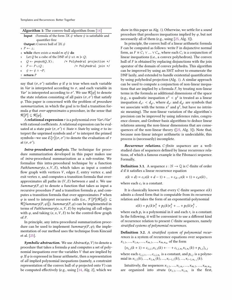
into CHORA’s invariant-generation capability, the recursivesuite is not an ideal test of that capability, because the suitecontains many benchmarks that can be proved safe by un-rolling (e.g., verifying that Ackermann’s function evaluatedat (2,2) is equal to 7). That is, many of these benchmarksdo not actually require an analyzer to perform invariantgeneration.We now discuss three benchmarks from the SV-COMP
suite that do give some insight into CHORA’s capabilities,in that they are non-linearly recursive benchmarks that re-quire an analyzer to perform invariant-generation. The Ack-ermann01 benchmark contains an implementation of thetwo-argument Ackermann function, and the benchmark as-serts that the return value of Ackermann is non-negativeif its arguments are non-negative; CHORA is able to prove
Templates and Recurrences: Better Together
int ackermann(intm, int n) {if (m == 0) { return n + 1; }if (n == 0) { return ackermann(m − 1, 1); }return ackermann(m − 1, ackermann(m,n − 1));
}assert(n < 0 | |m < 0 | | ackermann(m,n) >= 0)int hanoi(int n) {
if (n == 1) { return 1; }return 2 ∗ (hanoi(n − 1)) + 1;
}void applyHanoi(int n, int f rom, int to, int via) {
if (n == 0) { return; }counter++;applyHanoi(n − 1, f rom,via, to);applyHanoi(n − 1,via, to, f rom);
}counter = 0; applyHanoi(n, ...); assert(hanoi(n) == counter )int f91(int x) {
if (x > 100) return x − 10; else { return f91(f91(x + 11)) };}res = f 91(x); assert(res == 91 | | x > 101 && res == x − 10)
Figure 4. Source code for three programs from the SV-COMPsuite: Ackermann01, RecHanoi01, and McCarthy91
that this assertion holds. The RecHanoi01 benchmark con-tains a non-linearly recursive cost-model of the Tower ofHanoi problem, along with a linearly recursive function thatdoubles its return value and adds one at each recursive call.The assertion in recHanoi01 states that these two functionscompute the same value, and CHORA is able to prove thisassertion. (The other tools that we tested, namely ICRA, UA,UTaipain, and VIAP, were not able to prove this assertion.)The McCarthy91 benchmark contains an implementationof McCarthy’s 91 function, along with an assertion that thereturn value of that function, when applied to an argumentx , either (1) equals 91, or else (2) equals x − 10. CHORA isnot well-suited to prove this assertion because the assertedproperty is a disjunction, i.e., it describes the return valueusing two cases, whereas the hypothetical summaries usedby CHORA do not contain disjunctions. (ICRA, UA, UTaipan,and VIAP were all able to prove this assertion.)
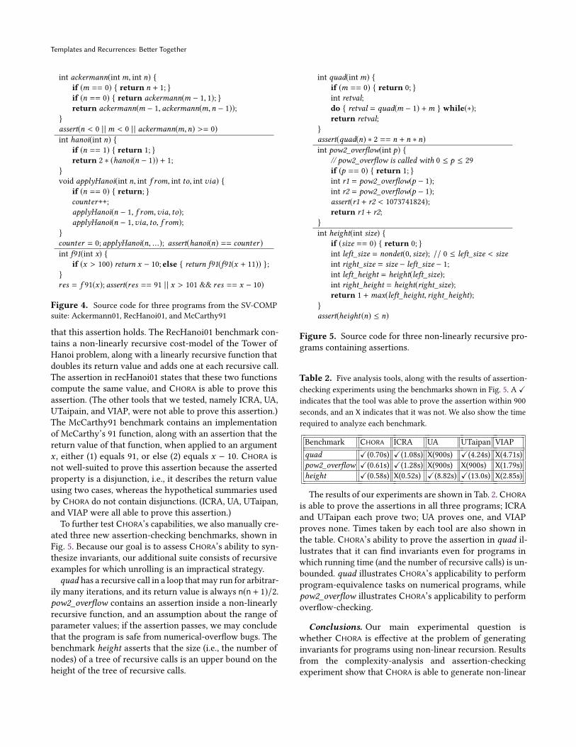
To further test CHORA’s capabilities, we also manually cre-ated three new assertion-checking benchmarks, shown inFig. 5. Because our goal is to assess CHORA’s ability to syn-thesize invariants, our additional suite consists of recursiveexamples for which unrolling is an impractical strategy.
quad has a recursive call in a loop that may run for arbitrar-ily many iterations, and its return value is always n(n+ 1)/2.pow2_overflow contains an assertion inside a non-linearlyrecursive function, and an assumption about the range ofparameter values; if the assertion passes, we may concludethat the program is safe from numerical-overflow bugs. Thebenchmark height asserts that the size (i.e., the number ofnodes) of a tree of recursive calls is an upper bound on theheight of the tree of recursive calls.
int quad(intm) {if (m == 0) { return 0; }int retval;do { retval = quad(m − 1) +m } while(∗);return retval;
}assert(quad(n) ∗ 2 == n + n ∗ n)int pow2_overflow(int p) {
// pow2_overflow is called with 0 ≤ p ≤ 29if (p == 0) { return 1; }int r1 = pow2_overflow(p − 1);int r2 = pow2_overflow(p − 1);assert(r1 + r2 < 1073741824);return r1 + r2;
}int height(int size) {
if (size == 0) { return 0; }int left_size = nondet(0, size); // 0 ≤ left_size < sizeint right_size = size − left_size − 1;int left_height = height(left_size);int right_height = height(right_size);return 1 +max(left_height, right_height);
}assert(heiдht(n) ≤ n)
Figure 5. Source code for three non-linearly recursive pro-grams containing assertions.
Table 2. Five analysis tools, along with the results of assertion-checking experiments using the benchmarks shown in Fig. 5. A ✓indicates that the tool was able to prove the assertion within 900seconds, and an X indicates that it was not. We also show the timerequired to analyze each benchmark.
Benchmark CHORA ICRA UA UTaipan VIAPquad ✓(0.70s) ✓(1.08s) X(900s) ✓(4.24s) X(4.71s)pow2_overflow ✓(0.61s) ✓(1.28s) X(900s) X(900s) X(1.79s)height ✓(0.58s) X(0.52s) ✓(8.82s) ✓(13.0s) X(2.85s)
The results of our experiments are shown in Tab. 2.CHORA
is able to prove the assertions in all three programs; ICRAand UTaipan each prove two; UA proves one, and VIAPproves none. Times taken by each tool are also shown inthe table. CHORA’s ability to prove the assertion in quad il-lustrates that it can find invariants even for programs inwhich running time (and the number of recursive calls) is un-bounded. quad illustrates CHORA’s applicability to performprogram-equivalence tasks on numerical programs, whilepow2_overflow illustrates CHORA’s applicability to performoverflow-checking.
Conclusions. Our main experimental question iswhether CHORA is effective at the problem of generatinginvariants for programs using non-linear recursion. Resultsfrom the complexity-analysis and assertion-checkingexperiment show that CHORA is able to generate non-linear
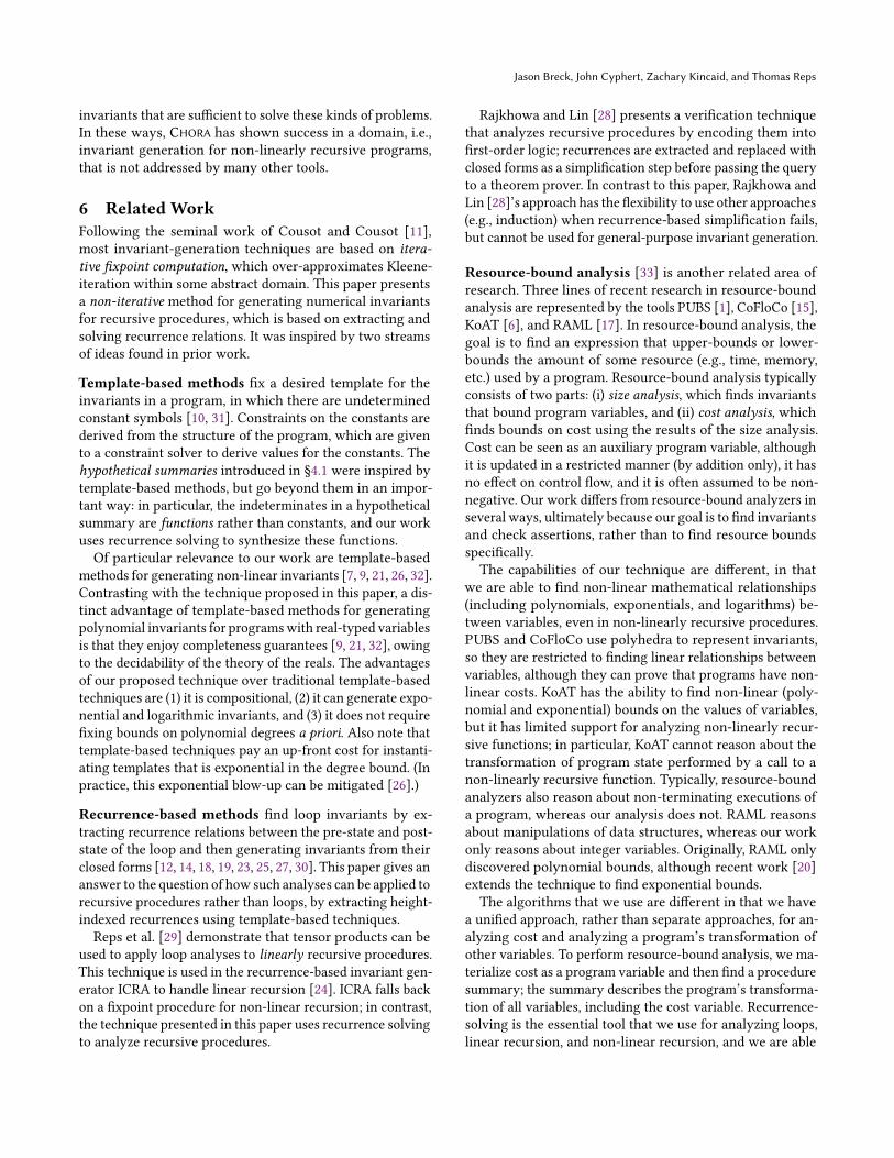
Jason Breck, John Cyphert, Zachary Kincaid, and Thomas Reps
invariants that are sufficient to solve these kinds of problems.In these ways, CHORA has shown success in a domain, i.e.,invariant generation for non-linearly recursive programs,that is not addressed by many other tools.
6 Related WorkFollowing the seminal work of Cousot and Cousot [11],most invariant-generation techniques are based on itera-tive fixpoint computation, which over-approximates Kleene-iteration within some abstract domain. This paper presentsa non-iterative method for generating numerical invariantsfor recursive procedures, which is based on extracting andsolving recurrence relations. It was inspired by two streamsof ideas found in prior work.
Template-based methods fix a desired template for theinvariants in a program, in which there are undeterminedconstant symbols [10, 31]. Constraints on the constants arederived from the structure of the program, which are givento a constraint solver to derive values for the constants. Thehypothetical summaries introduced in §4.1 were inspired bytemplate-based methods, but go beyond them in an impor-tant way: in particular, the indeterminates in a hypotheticalsummary are functions rather than constants, and our workuses recurrence solving to synthesize these functions.Of particular relevance to our work are template-based
methods for generating non-linear invariants [7, 9, 21, 26, 32].Contrasting with the technique proposed in this paper, a dis-tinct advantage of template-based methods for generatingpolynomial invariants for programswith real-typed variablesis that they enjoy completeness guarantees [9, 21, 32], owingto the decidability of the theory of the reals. The advantagesof our proposed technique over traditional template-basedtechniques are (1) it is compositional, (2) it can generate expo-nential and logarithmic invariants, and (3) it does not requirefixing bounds on polynomial degrees a priori. Also note thattemplate-based techniques pay an up-front cost for instanti-ating templates that is exponential in the degree bound. (Inpractice, this exponential blow-up can be mitigated [26].)
Recurrence-based methods find loop invariants by ex-tracting recurrence relations between the pre-state and post-state of the loop and then generating invariants from theirclosed forms [12, 14, 18, 19, 23, 25, 27, 30]. This paper gives ananswer to the question of how such analyses can be applied torecursive procedures rather than loops, by extracting height-indexed recurrences using template-based techniques.Reps et al. [29] demonstrate that tensor products can be
used to apply loop analyses to linearly recursive procedures.This technique is used in the recurrence-based invariant gen-erator ICRA to handle linear recursion [24]. ICRA falls backon a fixpoint procedure for non-linear recursion; in contrast,the technique presented in this paper uses recurrence solvingto analyze recursive procedures.
Rajkhowa and Lin [28] presents a verification techniquethat analyzes recursive procedures by encoding them intofirst-order logic; recurrences are extracted and replaced withclosed forms as a simplification step before passing the queryto a theorem prover. In contrast to this paper, Rajkhowa andLin [28]’s approach has the flexibility to use other approaches(e.g., induction) when recurrence-based simplification fails,but cannot be used for general-purpose invariant generation.
Resource-bound analysis [33] is another related area ofresearch. Three lines of recent research in resource-boundanalysis are represented by the tools PUBS [1], CoFloCo [15],KoAT [6], and RAML [17]. In resource-bound analysis, thegoal is to find an expression that upper-bounds or lower-bounds the amount of some resource (e.g., time, memory,etc.) used by a program. Resource-bound analysis typicallyconsists of two parts: (i) size analysis, which finds invariantsthat bound program variables, and (ii) cost analysis, whichfinds bounds on cost using the results of the size analysis.Cost can be seen as an auxiliary program variable, althoughit is updated in a restricted manner (by addition only), it hasno effect on control flow, and it is often assumed to be non-negative. Our work differs from resource-bound analyzers inseveral ways, ultimately because our goal is to find invariantsand check assertions, rather than to find resource boundsspecifically.The capabilities of our technique are different, in that
we are able to find non-linear mathematical relationships(including polynomials, exponentials, and logarithms) be-tween variables, even in non-linearly recursive procedures.PUBS and CoFloCo use polyhedra to represent invariants,so they are restricted to finding linear relationships betweenvariables, although they can prove that programs have non-linear costs. KoAT has the ability to find non-linear (poly-nomial and exponential) bounds on the values of variables,but it has limited support for analyzing non-linearly recur-sive functions; in particular, KoAT cannot reason about thetransformation of program state performed by a call to anon-linearly recursive function. Typically, resource-boundanalyzers also reason about non-terminating executions ofa program, whereas our analysis does not. RAML reasonsabout manipulations of data structures, whereas our workonly reasons about integer variables. Originally, RAML onlydiscovered polynomial bounds, although recent work [20]extends the technique to find exponential bounds.The algorithms that we use are different in that we have
a unified approach, rather than separate approaches, for an-alyzing cost and analyzing a program’s transformation ofother variables. To perform resource-bound analysis, we ma-terialize cost as a program variable and then find a proceduresummary; the summary describes the program’s transforma-tion of all variables, including the cost variable. Recurrence-solving is the essential tool that we use for analyzing loops,linear recursion, and non-linear recursion, and we are able

Templates and Recurrences: Better Together
to find non-linear mathematical relationships because suchrelationships arise in the solutions of recurrences.
AcknowledgmentsSupported, in part, by a gift from Rajiv and Ritu Batra; byONR under grants N00014-17-1-2889 and N00014-19-1-2318.The U.S. Government is authorized to reproduce and dis-tribute reprints for Governmental purposes notwithstandingany copyright notation thereon. Opinions, findings, conclu-sions, or recommendations expressed in this publication arethose of the authors, and do not necessarily reflect the viewsof the sponsoring agencies.
References[1] E. Albert, P. Arenas, and S. Genaim. 2011. Closed-Form Upper Bounds
in Static Cost Analysis. J. Autom. Reasoning (2011).[2] E. Albert, P. Arenas, S. Genaim, and G. Puebla. 2019. PUBS: A Practical
Upper Bound Solver. https://costa.fdi.ucm.es/pubs/examples.php[3] E. Albert, S. Genaim, and A. Masud. 2013. On the Inference of Resource
Usage Upper and Lower Bounds. In ACM. Trans. Comput. Logic.[4] J. Breck, J. Cyphert, Z. Kincaid, and T. Reps. 2020. CHORA repository.
https://github.com/jbreck/duet-jbreck[5] J. Breck, J. Cyphert, Z. Kincaid, and T. Reps. 2020. Templates and
Recurrences: Better Together. In PLDI. https://doi.org/10.1145/3385412.3386035
[6] M. Brockschmidt, F. Emmes, S. Falke, C. Fuhs, and J. Giesl. 2016. Ana-lyzing Runtime and Size Complexity of Integer Programs. ACM Trans.Program. Lang. Syst. (2016).
[7] David Cachera, Thomas Jensen, Arnaud Jobin, and Florent Kirchner.2012. Inference of Polynomial Invariants for Imperative Programs: AFarewell to Gröbner Bases. In SAS. 58–74.
[8] Q. Carbonneaux, J. Hoffmann, and Z. Shao. 2015. CompositionalCertified Resource Bounds. In PLDI.
[9] K. Chatterjee, H. Fu, and A. Goharshady. 2019. Non-polynomial Worst-Case Analysis of Recursive Programs. TOPLAS. (2019).
[10] M.A. Colón, S. Sankaranarayanan, andH. Sipma. 2003. Linear InvariantGeneration Using Non-Linear Constraint Solving. In CAV.
[11] P. Cousot and R. Cousot. 1977. Abstract Interpretation: A UnifiedLattice Model for Static Analysis of Programs by Construction orApproximation of Fixpoints. In POPL.
[12] S. de Oliveira, S. Bensalem, and V. Prevosto. 2016. Polynomial Invari-ants by Linear Algebra. In ATVA. 479–494.
[13] D. Dietsch, M. Greitschus, M. Heizmann, J. Hoenicke, A. Nutz, A.Podelski, C. Schilling, and T. Schindler. 2018. Ultimate Taipan withDynamic Block Encoding - (Competition Contribution). In TACAS.
[14] A. Farzan and Z. Kincaid. 2015. Compositional Recurrence Analysis.In FMCAD.
[15] Antonio Flores Montoya. 2017. Cost Analysis of Programs Based on theRefinement of Cost Relations. Ph.D. Dissertation. TU Darmstadt.
[16] M. Heizmann, J. Christ, D. Dietsch, E. Ermis, J. Hoenicke, M. Linden-mann, A. Nutz, C. Schilling, and A. Podelski. 2013. Ultimate Automizerwith SMTInterpol (Competition Contribution). In TACAS.
[17] J. Hoffmann, K. Aehlig, and M. Hofmann. 2012. Resource Aware ML.In CAV.
[18] A. Humenberger, M. Jaroschek, and L. Kovacs. 2017. Automated Gen-eration of Non-Linear Loop Invariants Utilizing Hypergeometric Se-quences. In ISSAC.
[19] A. Humenberger, M. Jaroschek, and L. Kovács. 2018. Invariant Gener-ation for Multi-Path Loops with Polynomial Assignments. In VMCAI.226–246.
[20] D. Kahn and J. Hoffmann. 2019. Exponential Automatic AmortizedResource Analysis. Technical Report. Carnegie Mellon University.
[21] Deepak Kapur. 2004. Automatically Generating Loop Invariants UsingQuantifier Elimination. In ACA.
[22] Manuel Kauers and Peter Paule. 2011. The Concrete Tetrahedron: sym-bolic sums, recurrence equations, generating functions, asymptotic esti-mates. Springer Science & Business Media.
[23] Z. Kincaid, J. Breck, J. Cyphert, and T. Reps. 2019. Closed Forms forNumerical Loops. In POPL.
[24] Z. Kincaid, J. Breck, A. Forouhi Boroujeni, and T. Reps. 2017. Compo-sitional Recurrence Analysis Revisited. In PLDI.
[25] Z. Kincaid, J. Cyphert, J. Breck, and T. Reps. 2018. Non-Linear Reason-ing for Invariant Synthesis. PACMPL 2(POPL) (2018), 54:1–54:33.
[26] Kensuke Kojima, Minoru Kinoshita, and Kohei Suenaga. 2016. Gener-alized Homogeneous Polynomials for Efficient Template-Based Non-linear Invariant Synthesis. In SAS.
[27] L. Kovács. 2008. Reasoning Algebraically About P-Solvable Loops. InTACAS.
[28] Pritom Rajkhowa and Fangzhen Lin. 2017. VIAP - Automated Systemfor Verifying Integer Assignment Programs with Loops. In SYNASC.
[29] T. Reps, E. Turetsky, and P. Prabhu. 2017. Newtonian ProgramAnalysisvia Tensor Product. TOPLAS. 39, 2, 9:1–9:72.
[30] E. Rodríguez-Carbonell and D. Kapur. 2004. Automatic Generation ofPolynomial Loop Invariants: Algebraic Foundations. In ISSAC. 266–273.
[31] S. Sankaranarayanan, H. Sipma, and Z. Manna. 2004. Constraint-BasedLinear-Relations Analysis. In SAS.
[32] Sriram Sankaranarayanan, Henny B. Sipma, and Zohar Manna. 2004.Non-linear Loop Invariant Generation Using GröBner Bases. In POPL.
[33] Ben Wegbreit. 1975. Mechanical program analysis. Commun. ACM(1975).

Jason Breck, John Cyphert, Zachary Kincaid, and Thomas Reps
A AppendixIn this section, we provide a detailed argument for the sound-ness of height-based recurrence analysis. We discuss the pro-cess of performing a height-based recurrence analysis onsome procedure P . The sequence of operations in that anal-ysis is as follows. First, Alg. 2 analyzes P , and produces asoutput a set of candidate recurrence inequations. On lines (1)–(6), Alg. 2 also produces a set {τi }i ∈[1,n] of two-vocabularyrelational expressions. Next, Alg. 3 filters down the set ofcandidate recurrences produced by Alg. 2 to obtain a strati-fied recurrence that can be solved by a C-finite recurrencesolver. Finally, a recurrence solver produces a solution in theform of a set of functions {bi }i ∈B , where B = {i1, ..., im} is asubset of the indices [1,n].In this discussion of soundness, we wish to relate the
functions {bi }i ∈B that are produced by the analysis to thesets of valuesVτ (P ,h) taken on by each relational expressionτi at each height h, which have the following definition interms of the relational semantics given in §3:
Vτ (P ,h)def= {EJτ K(σ ,σ ′) : (σ ,σ ′) ∈ R(P ,h)}.
WeuseVτ (P ,h) to prove a height-relative soundness propertyof our procedure summaries, which contain the height h asan explicit parameter. The fact that the summaries containan explicit representation of height means that they can bemade more precise by conjoining them to the depth-boundsummaries computed in §4.2.
The goal of this section is to prove the following soundnesstheorem.TheoremA.1. Let P be a procedure to which Alg. 2 and Alg. 3have been applied to obtain stratified recurrence. Let {τi }i ∈[1,n]be the relational expressions computed by Alg. 2. Let B ⊆ [1,n]be such that {bi }i ∈B is the set of functions produced by solvingthe stratified recurrence. Then, the following statement holds:∀h ≥ 1.
∧i ∈B ∀v ∈ Vτi (P ,h).v ≤ bi (h).
We will prove Thm. A.1 by induction on the height h.However, before the main inductive argument, we will pro-vide some definitions, and discuss the properties of Alg. 2,the recurrence-extraction algorithm Alg. 3, and the set offunctions {bi }i ∈B . (Note that the Alg. 3 referred to in thisappendix is not the same as the Alg. 3 that appears in theconference version [5] of this document, which appears asthe depth-bounding algorithm Alg. 4 in this technical reportversion.)
Define a feasible trace of a procedure P to be a finite list ofpairs of control locations and program states, starting at theentry location of P , ending at the exit location of P , in whichall the state transitions are consistent with the semanticsof P , and all calls are matched by returns. Note that thisdefinition only considers finite (i.e., terminating) traces of P ,which is useful because our ultimate goal is to find proceduresummaries that over-approximate a procedure’s pre-state-post-state relation, and a procedure only has a post-state
when it terminates. (As described below, we will also discussa modified version of P called P̂ , and we will consider thefeasible traces of P̂ to be only those that meet some additionalconstraints.) Furthermore, we define the feasible traces of Pup to height h to be those feasible traces that have a recursiondepth not exceeding h. For the following soundness proof,we define invariants of P to be properties that hold in allfeasible traces of P .
As explained above, the main function of Alg. 3 is to filterdown the set of candidate recurrence inequations producedby Alg. 2, to obtain a subset that constitute a stratified re-currence. At the end of that process, the inequations arechanged into equations so as to obtain the maximal solutionto the set of inequations. The output of Alg. 3 is a stratifiedrecurrence that can be written as:∧
i ∈Bbi (h + 1) = pi (bi1 (h), . . . ,bim (h)),
in which each pi (x1, . . . ,xm) is a polynomial in the variablesx1, . . . ,xm .
All coefficients in the polynomials {pi }i ∈B are non-negative, including the constant coefficients, as a result ofline (6) of Alg. 3, which drops terms having negative coef-ficients from the polynomial inequations that are given asinput to Alg. 3, thereby weakening the inequations. Asidefrom line (6), all other steps of Alg. 3 serve only to filter downthe set of candidate recurrences. Because of the droppingof terms having negative coefficients on line (6), the poly-nomials pi may differ from the corresponding polynomialsthat appeared in the input to Alg. 3; for each i ∈ B, we de-note by p ′i the corresponding polynomial in the input, beforeterms having negative coefficients were dropped. We referto the candidate inequations involving the p ′i polynomialsas the selected candidate inequations, because they are theones that are selected by Alg. 3 for inclusion in the stratifiedrecurrence (after their terms having negative coefficients aredropped).During the recurrence-solving phase, the zero vector is
used as the initial condition of the recurrence. Thus, theset of functions that occur as the solution to the recurrencesatisfy ∀i ∈ B,bi (1) = 0. Because all polynomials pi haveonly non-negative coefficients, the functions {bi (h)}i ∈B arenon-negative and non-decreasing for h ≥ 1.Our final digression before proving Thm. A.1 is a discus-
sion of Alg. 2. Alg. 2 operates by manipulating formulas thatinclude a set of function symbols named {bi (h)}i ∈[1,n] and{bi (h + 1)}i ∈[1,n]. The names of these symbols are the sameas those of the corresponding functions that are derived byrecurrence solving; however, in this proof, we will use sepa-rate names for the symbols manipulated by Alg. 2 and thecorresponding functions. Instead of bi (h) we will refer to thesymbol xi , and instead of bi (h + 1), we will refer to the sym-bol yi . Furthermore, although Alg. 2, as written, manipulatesformulas that are augmented with these additional symbols,

Templates and Recurrences: Better Together
it will be convenient in the following argument to take analternative, but equivalent, view, according to which Alg. 2analyzes a modified version of the procedure P called P̂ thatis obtained by making three changes to P .First, P̂ is augmented with a set of immutable auxiliary
variables named x1, ...,xn ,y1, ...,yn . Second, we impose aconstraint on the feasible traces of P̂ , namely that the pre-state σ and post-state σ ′ of any trace t of P̂ must satisfy theconstraint
∧ni=1(yi = EJτiK(σ ,σ ′)), or else t is not considered
to be a feasible trace of P̂ . This constraint is the equivalentof the formula-manipulation performed by line (9) of Alg. 2.Third, the recursive call sites in P are replaced with
control-flow edges that havoc their post-state σ ′ and ex-ecute assume(φcall). That is, the feasible executions of thesecontrol-flow edges of P̂ are all those in which the pre-state σ and post-state σ ′ of the control-flow edge satisfy∧n
i=1(EJτiK(σ ,σ ′) ≤ xi ∧ xi ≥ 0). The effect of replacing calledges of P in this way is equivalent to that of the formula-manipulation performed by line (7) of Alg. 2.Having described the above constraints on feasible ex-
ecutions of P̂ , we can now succinctly describe the outputof Alg. 2: each of the candidate recurrence inequations re-turned by Alg. 2 is an invariant of P̂ , i.e., a property thatholds in all feasible executions of P̂ . The soundness of theseinvariants follows from the soundness of the underlyingprogram-analysis primitives used by Alg. 2. For the proof ofThm. A.1, the crucial invariant of P̂ is the conjunction of theselected candidate inequations:
{yi ≤ p ′i (xi1 , ...,xim )}i ∈B . (18)We now begin the inductive proof of Thm. A.1.
Proof. The base case of the proof corresponds to a heightvalue of 1, which in turn corresponds to executions of thebase case of procedure P . At height 1, we must show:∧
i ∈B∀v ∈ Vτi (P , 1).v ≤ bi (1),
which holds because each relational expression τi was con-structed to be bounded above by zero in the base case, andeach bounding function bi evaluates to zero at height 1.
The inductive step of the proof is as follows. The inductivehypothesis states that, for some h,∧
i ∈B∀v ∈ Vτi (P ,h).v ≤ bi (h),
and the goal is to prove that∧i ∈B
∀v ∈ Vτi (P ,h + 1).v ≤ bi (h + 1).
Let t be any feasible trace of P at height up to h + 1. We willshow that we can modify the trace t to produce a new tracet̂ , and we then prove that t̂ is a feasible trace of P̂ .
To construct t̂ , first modify t to add the immutable auxil-iary variables x1, ...,xm ,y1, ...,ym to each program state in t .
We choose the values of these auxiliary variables as follows.Let σ and σ ′ be, respectively, the initial and final states of t .For each i ∈ [1,n], set yi to be the result of evaluating therelational expression τi using the state pair (σ ,σ ′), that is,yi = EJτiK(σ ,σ ′). Define the outermost recursive calls in thefeasible trace t to be the recursive calls to P that do not occurinside any other recursive call to P . Any feasible trace t is offinite length, and therefore t contains some finite number ofoutermost recursive calls. Thus, the set Ri,t of values takenon by τi evaluated at the pre-state/post-state pairs of eachoutermost recursive call in t is a finite set, and therefore wemay define Mi,t
def= max(0,max(Ri,t )) to be the maximum
value of τi occurring at any outermost recursive call in t .Now set each of the auxiliary variables xi as follows:
xi =
{bi (h) if i ∈ BMi,t otherwise
Finally, modify t̂ by collapsing all of the intermediate stepsof each outermost recursive call in t into a single state tran-sition, so as to match the replacement of recursive-call edgesof P with their corresponding edges in P̂ .We now argue that t̂ meets all the necessary constraints
to be considered a feasible trace of P̂ . The constraint on theinitial and final state of t̂ is that
∧ni=1(yi = τi ), which holds
by construction. The constraint at each outermost recursivecall of t is that, if (σ ,σ ′) are, respectively, the pre-state andthe post-state of the call, then
∧ni=1(EJτiK(σ ,σ ′) ≤ xi ∧ xi ≥
0). For i < B, xi = Mi,t , and each such Mi,t satisfies theconstraint by construction.For i ∈ B, xi = bi (h). We must show that xi is greater
than or equal to EJτiK(σ ,σ ′) and also greater than or equalto zero. Each xi is non-negative because each bi (h) is non-negative. By hypothesis, t is a feasible execution trace ofP at height h + 1. Thus, each outermost recursive call in tcorresponds to an execution of P of height at most h. (Notethat, if a trace is at height exactly h + 1, one of its recursivecalls must be at height exactly h, but the others may be atany height between 1 and h (inclusive).) Thus, the inductivehypothesis, ∧
i ∈B∀v ∈ Vτi (P ,h).v ≤ bi (h),
implies that the constraint relating xi to the value of τi ismet at each call. We conclude that the relevant constraintson t̂ are met, and therefore t̂ is a feasible trace of P̂ .As noted above, the output Alg. 2 is a set of invariants
of P̂ , i.e., properties that hold in all feasible traces of P̂ . Onesuch property is the conjunction of the selected candidateinequations shown in Eqn. (18). Let i ∈ B. We conclude thatthe ith selected candidate inequation holds in t̂ :
yi ≤ p ′i (xi1 , ...,xim )

Jason Breck, John Cyphert, Zachary Kincaid, and Thomas Reps
Let σ and σ ′ be the initial and final states of t̂ . By the con-struction of t̂ , we know that EJτiK(σ ,σ ′) = yi . Thus,
EJτiK(σ ,σ ′) ≤ p ′i (xi1 , ...,xim )By the construction of t̂ , we know that, for each k ∈ B,xk = bk (h). Thus,
EJτiK(σ ,σ ′) ≤ p ′i (bi1 (h), ...,bim (h))As noted above, each bi (h) is non-negative for any h ≥ 1.Thus, because p ′i and pi are being evaluated at non-negativearguments, and pi was derived from p ′i by dropping neg-ative coefficients, we conclude that p ′i (bi1 (h), ...,bim (h)) ≤pi (bi1 (h), ...,bim (h)) and therefore,
EJτiK(σ ,σ ′) ≤ pi (bi1 (h), ...,bim (h)). (19)The right-hand side Eqn. (19) matches the right-hand sideof the defining recurrence for bi , i.e., pi (bi1 (h), ...,bim (h)) =bi (h + 1). Thus,
EJτiK(σ ,σ ′) ≤ bi (h + 1).
Because we have shown this inequation to hold for eachi ∈ B, we conclude that∧
i ∈BEJτiK(σ ,σ ′) ≤ bi (h + 1). (20)
Recall that σ and σ ′ are the initial and final states of t̂ , andthat, by the construction of t̂ , these are also the initial andfinal states of the original trace t of P . But t was an arbitraryfeasible execution trace of P of height up to h + 1, and there-fore we conclude that Eqn. (20) holds if (σ ,σ ′) are the initialand final states of any feasible execution trace of P of heightup to h + 1. Thus,∧
i ∈B∀v ∈ Vτi (P ,h + 1).v ≤ bi (h + 1),
and the proof is complete. □