Tax Compliance: A BehavioralEconomics Approach

Thesis submitted for the degree of

Doctor of Philosophy

at the University of Leicester

by

Teimuraz GogsadzeDepartment of Economics

University of Leicester2016

To Megi and Marta

Tax Compliance: A Behavioral Economics Approach

by

Teimuraz Gogsadze

Abstract

Tax evasion is one of the key challenges for the policy makers. Designingthe optimal tax code requires assessment of taxpayers’ compliance behavior. Taxrate, detection intensity, penalty rate - are some of the characteristics consideredin models of tax evasion. The central question in tax evasion literature is howchanges in fiscal policy parameters affect evasion. The literature on tax evasioncan be categorized into two broad groups. The first strand of literature is based onexpected utility theory (EU) and the second strand approaches the evasion prob-lem from a behavioral perspective. This dissertation uses a behavioral approachto study tax compliance behavior and contributes to the second group of the liter-ature.

The second chapter of this dissertation investigates tax compliance behaviorof individuals with reference dependent preferences and endogenous referencepoint. The results are derived for the three personal equilibrium concepts ofKoszegi and Rabin (2007). The effects of tax policy parameters on complianceare found qualitatively similar to the results under EU.

Do taxpayers change their tax compliance behavior after the announcementand before the actual enforcement of a new tax rate? This is the central questionof the third chapter. Using cumulative prospect theory framework and a refer-ence point adaptation process, the answer is that evasion in the transition periodincreases following the announcement of the tax rate reduction or increase. An in-crease in the tax rate increases evasion, whereas reduction of the tax rate reducesevasion in the long run.

The final chapter of this dissertation develops a model of tax compliance be-havior with endogenous social norms. The implications of the model are that thetax policy parameters not only shape monetary (dis)incentives for compliance, butalso determine the strength of the social norm of compliance. The social norm ofcompliance is weaker under the higher tax rate and the norm is stronger underthe stricter tax enforcement regime.

Acknowledgments

First and foremost, I would like to express my sincere gratitude to my super-

visors Prof. Sanjit Dhami and Prof. Ali al-Nowaihi for the continuous support

throughout my Ph.D. study and for their patience, motivation, and encourage-

ment. I have been extremely fortunate to have supervisors who gave me the free-

dom to explore on my own, and at the same time guided me when I needed help.

I thank my university friends and fellows for the stimulating discussions, their

encouragement and all the fun we had during our Ph.D. journey. Junaid Arshad,

Sneha Gaddam, Evangelos Litos and Jingyi Mao deserve a special mention. I

highly value their friendship and I deeply appreciate their support during all these

years.

I am grateful to the administrative staff of economics department for their help

and support, especially Sebastian O’Halloran, Samantha Hill and Eve Danvers. I

must also thank the University of Leicester for granting me the graduate teaching

assistantship, without which my Ph.D. studies would not have been possible.

I would like to thank International School of Economics at Tbilisi State Univer-

sity and its director Eric Livny for supporting my Ph.D. applications at the initial

stage.

Last but not the least, I would like to thank my family for their love and en-

couragement: my parents, my brother and most of all my loving, patient and

supportive wife Megi. Four years ago, short after the start of my Ph.D., my daugh-

ter, Marta was born. Her presence has been filling me with enthusiasm that I had

never felt before. I would like to thank her for changing my life forever.

Contents

I General Introduction 1

II Tax Evasion with Endogenous Reference Point 3

1 Introduction 3

2 Framework of Stochastic and Endogenous Reference Points 6

3 The Model 11

4 Income Declaration as a CPE 13

5 Income Declaration as an UPE 20

6 Conclusion 30

III Tax Compliance in the Presence of Hedonic Adaptation 32

1 Introduction 32

2 Related Literature 34

3 A Note on Hedonic Adaptation 37

4 The Model 38

5 Static Solution 40

5.1 Stationary Case . . . . . . . . . . . . . . . . . . . . . . . . . . . . . 40

5.2 Tax Rate Reduction . . . . . . . . . . . . . . . . . . . . . . . . . . 41

5.2.1 Analysis of the Transition Period . . . . . . . . . . . . . . . 41

5.2.2 Analysis of the Enforcement Period . . . . . . . . . . . . . . 45

5.3 Tax Rate Increase . . . . . . . . . . . . . . . . . . . . . . . . . . . . 50

5.3.1 Analysis of the Transition Period . . . . . . . . . . . . . . . 50

5.3.2 Analysis of the Enforcement Period . . . . . . . . . . . . . . 54

6 Concluding Remarks 58

1

IV A Model of Tax Evasion with Endogenous Social Norms 60

1 Introduction 60

2 The Model 64

3 The Taxpayer’s Compliance Problem 67

4 Equilibrium Group Compliance and Social Norms 70

5 Concluding Remarks 73

2

List of Figures

1 UPE and CPE comparison . . . . . . . . . . . . . . . . . . . . . . . 25

2 Case 1 - Equilibrium tax compliance behavior under UPE . . . . . . 28

3 Case 2 - Equilibrium tax compliance behavior under UPE . . . . . . 29

4 Time flow . . . . . . . . . . . . . . . . . . . . . . . . . . . . . . . . 40

5 Optimal declaration in stationary and transition periods . . . . . . 45

6 Optimal declaration in transition and enforcement periods . . . . . 48

7 Optimal declaration in stationary and transition periods . . . . . . 53

8 Optimal declaration in transition and enforcement periods . . . . . 57

3

Chapter I

General IntroductionIn this dissertation I study tax compliance behavior of individuals with refer-

ence dependent preferences and address to the existing puzzles in the tax evasion

literature. Using a behavioral economics approach, I investigate the roles of expec-

tations, hedonic adaptation and social norms in a taxpayer’s compliance behavior.

Tax compliance, as a decision problem under uncertainty was first introduced

by Allingham and Sandmo (1972). In their model a taxpayer pays taxes on her

declared income. The tax authority does not observe the true income of the tax-

payer unless an audit is carried out, in which case the true income is learnt with

certainty. If the taxpayer is caught underreporting her income, she has to pay

the evaded taxes and a penalty. Tax evasion is successful, if an audit does not

occur. Therefore, the taxpayer decides what amount of income to declare given

the tax environment that is characterized by the tax rate, the penalty rate and the

probability of an audit. A simple and tractable setup of their model has clear-cut

predictions of the tax evasion behavior under expected utility theory (EU). For in-

stance, an increase in the probability of an audit and the penalty rate has deterrent

effects on evasion. Given the structure of the penalty, that is proportional to the

concealed income in the model, an increase in the tax rate has ambiguous effect

on evasion. Yitzhaki (1974) notes that in practice penalty is proportional to the

evaded taxes rather than the concealed income. Then using EU, under the em-

pirically plausible assumption of decreasing absolute risk aversion, an increase in

the tax rate reduces evasion at an interior optimum. This counter intuitive result,

known as Yitzhaki puzzle, is not supported by the majority of the empirical works

(e.g., Friedland et al., 1978; Clotfelter, 1983). In addition, by considering only

monetary (dis)incentives for compliance, the Allingham-Sandmo-Yitzhaki model

predicts too much evasion relative to the empirically observed levels and gener-

ates a puzzling question - why do people pay taxes (Alm et al., 1992; Alm and

Torgler, 2011)? The model fails to explain why some people never evade taxes.

In the second chapter, I study the Allingham-Sandmo-Yitzhaki model of tax

evasion using the decision theory of Koszegi and Rabin (2006, 2007). In their the-

ory, a reference point is determined by the expectations an individual held about

the outcomes in the recent past. I derive results for the three personal equilibrium

concepts of Koszegi and Rabin (2007) - choice-acclimating personal equilibrium

(CPE), unacclimating personal equilibrium (UPE) and preferred personal equi-

1

librium (PPE). I show that the comparative statics results under CPE and EU are

qualitatively similar. CPE , like EU, incorrectly predicts the compliance-tax rate

relation when the psychological cost of evasion is not part of the model and the

effect of the tax rate increase on evasion turns ambiguous following the introduc-

tion of the psychological cost of evasion. Therefore, CPE cannot solve the Yitzhaki

puzzle. Nonetheless, unlike EU, CPE can explain why some taxpayers never evade

and it predicts higher compliance levels compared to EU. Under UPE , the effects

of the tax policy parameters are also qualitatively similar to those under CPE and

EU. In the existence of multiple UPE , the concept of PPE is used to investigate

the equilibrium tax compliance behavior of taxpayers.

The third chapter investigates tax compliance behavior of a taxpayer in an

environment, where the announcement of a tax rate change precedes the actual

enforcement. The work explores cumulative prospect theory-based tax evasion

model in the presence of hedonic adaptation. It shows that, under some conditions,

evasion in the transition period increases following the announcement of the tax

rate reduction or increase. The anticipation of tax changes does not incentivize

full tax evaders to revise their declaration decision during the transition period

and only the behavior of some fully compliant taxpayers is found to be affected

by the announcement. The enforcement of a new tax rate is found to have long

run effects on evasion - an increase in the tax rate increases evasion, whereas

reduction of the tax rate reduces evasion in the long run.

The final chapter of this dissertation develops a model of tax compliance behav-

ior with endogenous social norms in the prospect theory framework. The model

rests on the following assumptions. First, the strength of the social norm of com-

pliance depends on the overall extent of evasion. Second, taxpayers identify them-

selves with a group of individuals with the same income levels and internalize the

norms that are attributed to this group. Third, taxpayers are guilt averse in the

social domain of their preferences. The implications of the model are that the tax

policy parameters not only shape monetary (dis)incentives for compliance, but

also determine the strength of the social norm of compliance at the equilibrium.

An increase in the tax rate is found to weaken the norm of compliance, whereas

stricter tax enforcement regime strengthens the norm of compliance.

2

Chapter II

Tax Evasion with EndogenousReference Point

1 Introduction

The leading decision theory in neoclassical economics, expected utility theory

(EU), has been found inconsistent with numerous empirical phenomena. Among

others, EU has generated several puzzles in the tax evasion literature.

Tax compliance, as a decision problem under uncertainty was first introduced

by Allingham and Sandmo (1972) in the economics-of-crime framework of Becker

(1968). In their model a taxpayer pays taxes on her declared income. The tax

authority does not observe the true income of the taxpayer unless an audit is

carried out, in which case the true income is learnt with certainty. If the tax-

payer is caught underreporting her income, she has to pay the evaded taxes and

a penalty. Tax evasion is successful, if an audit does not occur. Therefore, the

taxpayer decides what amount of income to declare given the tax environment

that is characterized by the tax rate, the penalty rate and the probability of an

audit. A simple and tractable setup of their model has clear-cut predictions of the

tax evasion behavior under EU. For instance, an increase in the probability of de-

tection and the penalty rate has deterrent effects on evasion. Given the structure

of the penalty, that is proportional to the concealed income in the model, an in-

crease in the tax rate has ambiguous effect on evasion. Yitzhaki (1974) notes that

in practice penalty is proportional to the evaded taxes rather than the concealed

income. Then using EU, under the empirically plausible assumption of decreasing

absolute risk aversion, an increase in the tax rate reduces evasion at an interior

optimum. This counter intuitive result, known as Yitzhaki puzzle, is not supported

by the majority of the empirical works (e.g., Friedland et al., 1978; Clotfelter,

1983). In addition, by considering only monetary (dis)incentives for compliance,

the Allingham-Sandmo-Yitzhaki model predicts too much evasion relative to the

empirically observed levels and generates a puzzling question - why do people

pay taxes? (Alm et al., 1992; Alm and Torgler, 2011)1 Therefore the model fails

1The empirical estimates of the probability of an audit, p, take values from 0.01 to 0.03, whilethe penalty rate, λ, that is paid in addition to the reimbursement of the evaded taxes, ranges from0.5 to 2 (see e.g., Dhami and al-Nowaihi, 2007). For these parameter values, the model predictsthat virtually all taxpayers evade some taxes as long as the expected return on evasion, 1− p− pλ,

3

to explain why some people never evade taxes.

Based on the refutations of EU, numerous alternative decision theories have

emerged. In this respect, prospect theory of Kahneman and Tversky (1979) and

cumulative prospect theory of Tversky and Kahneman (1992)2 have revolutionized

the field. Prospect theory (PT) and cumulative prospect theory (CP) are built on

the four main blocks: reference dependence, loss aversion, diminishing sensitivity

and non-linear weighting of probabilities. Dhami and al-Nowaihi (2007) use CP

to study the tax compliance problem and successfully solve the Yitzhaki puzzle.

Specifically, the authors find that at an interior optimum tax evasion increases in

the tax rate.

Other notable alternatives of EU include rank-dependent utility theory (Quig-

gin,1982; 1993), regret theory (Bell, 1982; Loomes and Sugden, 1982) and the

theory of disappointment aversion (Bell, 1985; Loomes and Sugden, 1986; Gul,

1991). Rank-dependent utility theory (RDU) uses classical utility function and

replaces objective probabilities with decision weights, which are derived using

a probability weighting function. Eide (2001) studies the Allingham-Sandmo-

Yitzhaki model of tax evasion using RDU and finds that the Yitzhaki puzzle is still

in place. Hence, reference dependence and loss aversion appear crucial to reverse

the compliance-tax rate relation.

Regret and disappointment are similar reference-effect phenomena by their na-

ture. Regret arises from the ex-post feeling of not having made the right choice,

whereas disappointment is incurred when the received outcome turns out smaller

than expected. It turns out that RDU is linked with disappointment aversion mod-

els in special cases. For instance, Delquié and Cillo (2006) develop a disappoint-

ment model, where a received outcome is compared with other individual out-

comes of a lottery. Assuming linearity of disappointment and elation functions,

the model leads to the rank-dependent representation of the preferences.

More recent theory, developed by Koszegi and Rabin (2006, 2007), henceforth

KR, generalizes prospect theory and links it with disappointment aversion models.

In KR framework utility is separable in two components - utility from the final con-

sumption, termed as ‘consumption utility’ and ‘gain-loss utility’. The latter is de-

rived from the comparison of consumption utility from the received outcome with

consumption utility from the reference point. Gain-loss utility shares the proper-

ties of the prospect theory value function, exhibiting diminishing sensitivity, loss

aversion and reference dependence. KR theory specifies the source of a reference

is positive.2The main difference between these two theories lies in the formation of decision weights.

4

point formation. A reference point is assumed to be shaped by the expectations

an individual held about the outcomes in the recent past. The expectations-based

reference point makes KR theory part of the disappointment literature.

KR theory has gained substantial empirical support. Abeler et al. (2011) con-

duct a real-effort experiment, where subjects can earn a fixed amount or an effort-

proportional amount with equal probabilities. The study finds that the effort pro-

vision increases in the fixed amount that is set by the experimenter and the finding

is explained by the expectations-based reference point. Ericson and Fuster (2011)

show that reference points are determined by expectations. In their experiment

subjects are endowed with an item and exposed to the probabilistic opportunity

to exchange their items for an alternative. The subjects are found more likely to

keep their items when the probability of exchange is low. Gill and Prowse (2012)

test KR theory and find supportive evidence for the expectations-based reference

point. In their experiment subjects perform real effort tasks in a competitive envi-

ronment. An effort chosen by the first mover is observed by the second mover who

then decides how hard to work. The authors find that an effort chosen by the sec-

ond mover depends on the effort provided by the first mover, which is explained

by the KR preferences. Crawford and Meng (2011) use KR theory to explain New

York taxi drivers’ labor supply.

Motivated by the increasing empirical support of KR theory, this chapter stud-

ies the tax compliance behavior of a taxpayer with reference-dependent prefer-

ences of KR-type. Three equilibrium concepts of KR theory are investigated in the

standard tax evasion model. The first concept, choice-acclimating personal equi-

librium (CPE), is used in an environment where decisions are made sufficiently

in advance of the resolution of uncertainty. The second concept, unacclimating

personal equilibrium (UPE) applies to an environment where a decision maker

makes her decision close to the resolution of uncertainty and the third concept,

preferred personal equilibrium (PPE), is used in the existence of multiple UPE .

The chapter shows that the comparative statics results under CPE are qualitatively

similar to the results under EU. Therefore, CPE cannot explain the Yitzhaki puzzle.

Nevertheless, CPE can explain why some people never evade taxes and predicts

higher compliance levels compared to EU. Under UPE , the effects of the tax policy

parameters are also qualitatively similar to those under CPE and EU. In the exis-

tence of multiple UPE , the concept of PPE is used to investigate the equilibrium

tax compliance behavior of taxpayers.

The rest of the chapter is structured as follows. Section 2 provides the basic

framework of KR theory. Section 3 outlines the tax evasion model. Section 4

5

considers tax evasion under CPE . Section 5 considers tax evasion under UPE and

Section 6 concludes.

2 Framework of Stochastic and Endogenous Refer-

ence Points

Koszegi and Rabin (2006) develop a general model of reference-dependent pref-

erences under uncertainty. The basic framework of their model is as follows.

An individual’s utility depends on the consumption level c ∈ R and the refer-

ence level r ∈ R, that captures beliefs of the person about the possible outcomes.

The utility from the final consumption level m(c), termed as ‘consumption utility’,

is the classical outcome-based utility. Utility from c with respect to the reference r

is termed as ‘gain-loss utility’ and it is denoted by n(c|r).3 An individual’s overall

utility is the sum of consumption and gain-loss utilities:

u(c|r) = m(c) + n(c|r) (2.1)

Uncertainty about the consumption outcome is characterized by the cumulative

distribution function F (c). If the reference point r is deterministic, then expected

utility of the consumption lottery is given by the following:

U(F |r) =

∫u(c|r) dF (c) (2.2)

The reference point may also be stochastic. Suppose an individual, who is fac-

ing uncertain consumption outcomes, has a stochastic reference point, or equiv-

alently - a reference lottery, that is characterized by the cumulative distribution

G(r). Then the individual’s expected utility of the consumption lottery, conditional

on the stochastic reference point, is given by the following:

U(F |G) =

∫ ∫u(c|r) dG(r) dF (c) (2.3)

An individual compares the realized consumption outcome with all possible

outcomes under the reference lottery. Each pairwise comparison yields sensation

of either gain or loss. For example, if the reference lottery is a gamble between

£10 and £20, then the outcome of £15 feels like a gain relative to £10 and a loss

relative to £20.3In the general model, consumption bundle is multidimensional and both components of the

utility, m and n, are additively separable across the dimensions.

6

Gain-loss utility is tightly related with consumption utility in the following

form:

n(c|r) = µ(m(c)−m(r)) (2.4)

Gain-loss utility, µ(·), has the following properties:

1. µ(x) is continuous for all x, twice differentiable for all x 6= 0 and strictly

increasing.

2. Reference dependence: µ(0) = 0.

3. Large stakes loss aversion: For y > x > 0, µ(y)− µ(x) < µ(−x)− µ(−y).

4. Small stakes loss aversion: Loss aversion parameter θ > 1 is equal to µ′−(0)

µ′+(0)

,

where µ′+(0) = limx→0+ µ′(x) and µ′−(0) = limx→0− µ

′(x).

5. Diminishing Sensitivity: µ′′(x) ≤ 0 for x > 0 and µ

′′(x) ≥ 0 for x < 0.4

The following linear form has been found to be adequate for small stake gam-

bles:

µ(x) =

ηx if x ≥ 0

ηθx if x < 0(2.5)

In this formulation, η > 0 is the weight an individual attaches to gain-loss utility

and θ > 1 is the loss aversion parameter.

For illustration purposes, consider the following example of a person with

reference-dependent preferences of KR-type.

Example 2.1 An individual faces an uncertain future. Suppose the realized con-sumption level can be either c1 or c2 and c1 < c2. The low consumption level, c1, isrealized with probability p and the high consumption level, c2, is realized with proba-bility (1− p). Hence, the consumption lottery is L = (c1, p; c2, 1− p). Denote by F theprobability distribution of consumption levels. Uncertainty about the future inducesthe stochastic reference point r, which takes two values, r1 with probability q and r2

with probability (1− q). Hence, the reference lottery is r = (r1, q; r2, 1− q). Denote byG the probability distribution of reference levels. Then using (2.3), expected utility ofthe lottery is given by the following:

U(F |G) = p[qu(c1|r1) + (1− q)u(c1|r2)] (2.6)

+(1− p)[qu(c2|r1) + (1− q)u(c2|r2)]

4The properties of gain-loss utility correspond to the properties of the prospect theory valuefunction.

7

The explanation of (2.6) is as follows. With probability p the realized outcome isc1. When c1 is realized, the individual compares it with r1 and r2 separately andthe derived utilities are weighted with probabilities q and (1 − q), respectively. Withprobability (1− p) the realized outcome is c2 and the pairwise comparisons with thereference outcomes are conducted in the similar manner. Substitution of (2.1) in(2.6) gives:

U(F |G) = pm(c1) + (1− p)m(c2) (2.7)

+ p[qn(c1|r1) + (1− q)n(c1|r2)]

+ (1− p)[qn(c2|r1) + (1− q)n(c2|r2)]

The first term in (2.7) is expected consumption utility and the second term is expectedgain-loss utility. Further substitution of (2.4) in (2.7) yields:

U(F |G) = pm(c1) + (1− p)m(c2) (2.8)

+ p[qµ(m(c1)−m(r1)) + (1− q)µ(m(c1)−m(r2))]

+ (1− p)[qµ(m(c2)−m(r1)) + (1− q)µ(m(c2)−m(r2))]

In the model a reference point is fully determined by the expectations an indi-

vidual held in the recent past. Koszegi and Rabin (2006) assume that the stochas-

tic reference point of an individual is her rational expectations about the possible

outcomes. The expectations are rational if a person correctly predicts the set of

outcomes and their probabilities. In Example 2.1, this implies that the reference

lottery coincides with the consumption lottery L = (c1, p; c2, 1− p) and hence, the

equivalent of (2.6) can be written as follows:

U(F |F ) = p[pu(c1|c1) + (1− p)u(c1|c2)] (2.6′)

+ (1− p)[pu(c2|c1) + (1− p)u(c2|c2)]

The equivalent of (2.7) is the following:

U(F |F ) = pm(c1) + (1− p)m(c2) (2.7′)

+ p[pn(c1|c1) + (1− p)n(c1|c2)]

+ (1− p)[pn(c2|c1) + (1− p)n(c2|c2)]

Observe that n(c1|c1) = n(c2|c2) = 0 because of the 2nd property of gain-loss utility

8

in (2.4). Taking this into account, the equivalent of (2.8) would be:

U(F |F ) = pm(c1) + (1− p)m(c2) (2.8′)

+ p(1− p)µ(m(c1)−m(c2))]

+ (1− p)pµ(m(c2)−m(c1))

(2.8′) describes an individual’s expected utility of the lottery with rational ex-

pectations as her reference point.

Having already described the preferences of an individual, next we consider

decision making under uncertainty. To shed light on this issue, I review the main

ideas of the follow-up paper by Koszegi and Rabin (2007). In this paper the au-

thors introduce three concepts of personal equilibrium. The concepts are defined

depending on how far from the resolution of uncertainty a decision maker makes

her decision.

We might find it useful to consider utility over wealth levels instead of con-

sumption levels, i.e., equivalent of (2.1) would be u(w|r) = m(w) + n(w|r), where

w stands for the wealth level and r is the reference wealth.

First consider a scenario, where a decision maker correctly predicts the choice

set but cannot make the committed choice until shortly before the resolution of

uncertainty. Because the decision is made in a short time period, a reference point

of the decision maker is a carrier of the past information and it is unchangeable.

That is, the expectations are given to her and the choice she makes does not affect

those expectations. Hence, the decision maker makes her optimal choice given

the expectations. In this case the respective equilibrium concept is unacclimating

personal equilibrium (UPE).

Suppose a decision maker is facing the compact choice set D ⊂ ∆(R). Each ele-

ment of the choice set is a probability distribution over the wealth levels. Suppose

a selection F ∈ D is the choice made by the decision maker. Then the definition

of UPE follows:

Definition 2.1 A selection F ∈ D is an unacclimating personal equilibrium (UPE)if for any F ′ ∈ D, U(F |F ) ≥ U(F

′|F ).

Therefore, according to Definition 2.1, if a decision maker expects to choose F

from the choice set D, she should indeed find it optimal to choose F. The optimal-

ity of meeting her expectations justifies the rationality of those expectations. At

UPE a decision maker does not maximize ex-ante expected utility among the avail-

able options as it is the case at choice-acclimating personal equilibrium (CPE),

9

that we define below. Rather, at UPE a choice is optimal given expectations at the

time of decision making.

To make the concept of UPE clearer, consider the following example.

Example 2.2 A decision maker is facing the choice set D = L = (w − 50, 12; w, 1

2),

I = w − 25. She can either choose the lottery of loosing £50 from her currentwealth with probability 1

2or buy an insurance for £25. Suppose the decision maker

expects to buy the insurance. Hence, she has a deterministic reference point that isequal to (w − 25). According to Definition 2.1, buying the insurance is an UPE ifU(I|I) ≥ U(L|I). Then using (2.1), (2.3) and (2.4), we have:

U(I|I) = m(w − 25) ≥ U(L|I) (2.9)

=1

2[m(w − 50) + µ(m(w − 50)−m(w − 25))]

+1

2[m(w) + µ(m(w)−m(w − 25))]

For simplicity assume m(x) = x. Then from (2.9) follows:

w − 25 ≥ 1

2[w − 50 + µ(−25)] +

1

2[w + µ(25)] (2.10)

=⇒ 0 ≥ µ(−25) + µ(25)

that is true given the property of gain-loss utility µ(·), that losses bite more than gainsof the same magnitude.

If a decision maker has multiple self-fulfilling expectations, there might be mul-

tiple UPE yielding different expected utilities. In this case, Koszegi and Rabin

(2007) assume that a decision maker chooses the UPE with the highest expected

utility. Such selection is defined as a preferred personal equilibrium (PPE).

Definition 2.2 A selection F ∈ D is a preferred personal equilibrium (PPE) if itis an UPE and U(F |F ) ≥ U(F

′|F ′) for all UPE selections F ′ ∈ D.

Now consider a situation, where a decision maker makes her decision a long

time before the resolution of uncertainty. In this case the committed decision

is incorporated into the reference point. Therefore, the expectations relative to

which outcomes are evaluated are influenced by the decision itself. The concept

of choice-acclimating personal equilibrium (CPE) applies to this case.

Definition 2.3 A selection F ∈ D is a choice-acclimating personal equilibrium

(CPE) if U(F |F ) ≥ U(F′ |F ′) for all F ′ ∈ D.

10

Unlike to UPE , at CPE a person makes her overall favorite choice. Returning

to Example 2.2, buying the insurance is a CPE if U(I|I) ≥ U(L|L). That is:

U(I|I) = u(w − 25|w − 25) ≥ U(L|L) (2.11)

=1

2

1

2u(w − 50|w − 50) +

1

2u(w − 50|w)

+

1

2

1

2u(w|w − 50) +

1

2u(w|w)

Using (2.1), (2.4) and the property µ(0) = 0, we get:

m(w − 25) ≥ (2.12)

1

2

1

2m(w − 50) +

1

2[m(w − 50) + µ(m(w − 50)−m(w))]

+

1

2

1

2[m(w) + µ(m(w)−m(w − 50))] +

1

2m(w)

Combining the terms in (2.12) gives:

m(w − 25) ≥ 1

2m(w − 50) +

1

2m(w) (2.13)

+ 1

4µ(m(w − 50)−m(w))

+1

4µ(m(w)−m(w − 50))

If we allow consumption utility to be linear, m(x) = x, then (2.13) is simplified to

the following:

0 ≥ µ(−50) + µ(50) (2.14)

which holds for a loss averse individual.

3 The Model

This section describes a model of tax evasion decision of an individual with ref-

erence dependent preferences and endogenous reference point. The setup of the

model follows the basic Allingham-Sandmo-Yitzhaki framework, enriched with the

consideration of the psychological cost of evasion.

A taxpayer has exogenously given income level, W, not directly observable by

the tax authority. Her declared income, D, is taxable at the proportional rate

11

t, such that 0 < t < 1. The taxpayer complies with the law if she declares full

income for taxation purposes, i.e., D = W, otherwise she evades some income,

i.e., 0 ≤ D < W . The taxpayer is audited with exogenously given probability,

0 < p < 1, and when audited, her actual income is discovered without an error.

If the taxpayer is detected evading, she has to pay evaded taxes, t[W −D], and a

penalty that is proportional to the evaded taxes, λt[W − D], where λ > 0 is the

penalty rate. Therefore, the disposable income of a non-audited taxpayer is given

by the following:

YNA = W − tD (3.1)

When a taxpayer is audited, her disposable income is:

YA = [1− t]W − λt[W −D] (3.2)

I assume that a taxpayer is not left penniless in any possible circumstances, i.e.,

1− t− λt > 0.

If a taxpayer is audited and caught evading, she suffers from social stigma. A

taxpayer has an individual-specific stigma rate, s, and the total stigma suffered

is proportional to the concealed income, i.e., s(W − D). 5 There is a continuum

of taxpayers who are identical in all respects apart from stigma, which has dis-

tribution function F (s) and support [0, S]. An individual derives utility from the

disposable income and disutility from being caught evading. A taxpayer has the

following quasilinear consumption utility function:

v(Yi, s) = u(Yi)− d× s(W −D) (3.3)

where i = A stands for audit outcome, i = NA stands for non-audit outcome and

u(Yi) is the utility derived from the disposable income. The utility function of the

pecuniary outcome is assumed to be twice differentiable, strictly increasing and

strictly concave, i.e., u′(Yi) > 0 and u′′(Yi) < 0. d is the auditing dummy variable

such that:

d =

1 if i = A

0 if i = NA

The reference-dependent preferences of a taxpayer is assumed to be of KR-type.

The total utility derived from an outcome is given by the following form:

V (Y, s|R) = v(Y, s) + µ(v(Y, s)− v(R, s)) (3.4)

5The formulation of stigma is similar to the one used by Gordon (1989).

12

where V (Y, s|R) is the utility derived from Y, given stigma and conditional on the

reference point R. v(Y, s) is consumption utility defined in (3.3). µ(x) is gain-loss

utility, identical to (2.5), where θ > 1 is the coefficient of loss aversion and η > 0

is the weight attached to gain-loss utility:

µ(x) =

ηx if x ≥ 0

ηθx if x < 0(3.5)

I solve the model for the three equilibrium concepts of Koszegi and Rabin

(2007): CPE , UPE and PPE . At first I consider a scenario where decisions are

made sufficiently in advance of the realization of an outcome and a decision maker

has enough time to get acclimatized to her decision. In this case, the relevant equi-

librium concept is choice-acclimating personal equilibrium (CPE).6 Afterwards, I

consider a scenario where a decision maker takes her decision too close to the

resolution of uncertainty. In this case, the relevant equilibrium concept is unaccli-

mating personal equilibrium (UPE).7 In case of multiple UPE , I use the concept

of preferred personal equilibrium (PPE).8

4 Income Declaration as a CPE

Consider an environment, where a taxpayer makes a committed declaration deci-

sion sufficiently in advance of the realization of an audit outcome. Therefore, the

taxpayer has enough time to get acclimatized to her decision. Then, she regards

her choice as a reference point by the time of the audit outcome realization.

The choice set of a taxpayer is the interval [0,W ]. Suppose she commits herself

to declaring D from the choice set. Then her stochastic reference point, that is

determined by the assumption of rational expectations, coincides with her choice

and is given by the following:

R =

YNA with probability (1− p)YA with probability p

(4.1)

where YNA and YA are given in (3.1) and (3.2), respectively.

If a taxpayer declares full income, then her reference point is deterministic and

equal to the legal after-tax income, YL = (1 − t)W. The deterministic reference

point is a special case of the stochastic reference point.

6Definition 2.37Definition 2.18Definition 2.2

13

An individual evaluates her choice in the following manner. She expects the

no-audit outcome, YNA, with probability (1−p). If the taxpayer is not audited, she

derives consumption utility from the realized outcome and gain-loss utility. The

latter is a consequence of pairwise comparison of consumption utility from the out-

come with consumption utilities from individual reference levels of the stochastic

reference point. A rational taxpayer expects an audit and the corresponding out-

come, YA, with probability p. Respective consumption and gain-loss utilities are

also derived for this case. That is, using (3.4) and (4.1), expected utility from the

choice vector Y is given by the following:

V (Y, s|Y ) = (1− p)v(YNA, s) + (1− p)µ(v(YNA, s)− v(YNA, s)) (4.2)

+ pµ(v(YNA, s)− v(YA, s))+ pv(YA, s)

+ (1− p)µ(v(YA, s)− v(YNA, s)) + pµ(v(YA, s)− v(YA, s))

Substitution of (3.3) into (4.2) yields:

V (Y, s|Y ) = (1− p)u(YNA) + (1− p)µ(0) (4.2′)

+ pµ(u(YNA)− u(YA ) + s(W −D))+ pu(YA )− s(W −D)

+ (1− p)µ(u(YA )− s(W −D)− u(YNA)) + pµ(0)

Using gain-loss utility in (3.5), we get:

V (Y, s|Y ) = (1− p) u(YNA) + pη[u(YNA)− u(YA ) + s(W −D)] (4.3)

+p u(YA )− s(W −D) + (1− p)ηθ[u(YA )− s(W −D)− u(YNA)]

Combining the terms in (4.3) gives:

V (Y, s|Y ) = [(1− p)− p(1− p)η(θ − 1)]× u(YNA) (4.4)

+[p+ p(1− p)η(θ − 1)]× [u(YA )− s(W −D)]

Using Definition 2.3, a selection D ∈ [0,W ] is a CPE if it is a maximizer of

(4.4). Since V (Y, s|Y ) is a continuous function of D on the non-empty compact

interval [0,W ], it attains a maximum at some D∗ ∈ [0,W ]. It turns out that a

taxpayer’s maximization problem under CPE is similar to a RDU maximization

problem. Unlike RDU, that uses a probability weighting function to derive decision

weights for outcomes, from (4.4) we see that the decision weights under CPE

14

depend on the objective probability of an audit, p, the loss aversion parameter, θ,

and the weight an individual attaches to gain-loss utility, η.9 The decision weights

add up to 1, i.e.,

[(1− p)− p(1− p)η(θ − 1)] + [p+ p(1− p)η(θ − 1)] = 1 (4.5)

The emergence of decision weights in KR theory is totally due to the loss aversion

parameter and the weight given to gain-loss utility. For instance, if an individual is

not loss averse, i.e., θ = 1, or she does not care about gains and losses, i.e., η = 0,

then we are back to EU. Hence, KR theory implicitly specifies the source of decision

weights and, unlike RDU, decision weights can be negative. From (4.4), for any

θ > 1 and η > 0, a decision weight given to the audit outcome is positive and

bigger than the objective probability of an audit, i.e., p+ p(1− p)η(θ− 1) > p > 0.

A decision weight attached to the no-audit outcome can be non-positive. The

following proposition considers a CPE declaration of a taxpayer, giving a non-

positive decision weight to the no-audit outcome.

Proposition 4.1 Suppose η ≥ 1p(θ−1)

, then the full income declaration, D = W, is theonly CPE .

Proof. If a taxpayer attaches sufficiently high weight to gain-loss utility, ulti-

mately she assigns a non-positive decision weight to the no-audit outcome, i.e.,

η ≥ 1p(θ−1)

⇐⇒ [(1− p)− p(1− p)η(θ − 1)] ≤ 0. First suppose η > 1p(θ−1)

. Then, the

maximization of (4.4) requires the minimization of u(YNA) and the maximization

of [u(YA ) − s(W − D)]. Using (3.1) and (3.2) and the property u′(Yi) > 0, (4.4)

attains its maximum at D = W . Next suppose η = 1p(θ−1)

. In this case, the maxi-

mization of (4.4) is equivalent to the maximization of [u(YA )− s(W −D)], which

occurs at D = W. Hence, when η ≥ 1p(θ−1)

, the full income declaration is the only

CPE .

Thus KR-theory can explain why some taxpayers never evade. It follows that,

assigning a strictly positive decision weight to the no-audit outcome is a necessary

condition for the emergence of tax evasion as a CPE . I consider this condition

next. Suppose a taxpayer assigns a positive decision weight to the no-audit out-

come, i.e., 0 < η < 1p(θ−1)

. Because the decision weights add up to 1, it follows that

0 < [(1−p)−p(1−p)η(θ−1)] < 1 and 0 < [p+p(1−p)η(θ−1)] < 1. Hence, a decision

9In this respect, CPE is similar to the disappointment aversion model of Delquié and Cillo(2006), which also results in the rank-dependent representation of the preferences.

15

maker overweights the probability of an audit, p, and underweights the probabil-

ity of no-audit occurrence, (1− p).10 Thus KR-theory, unlike RDU or PT, introduces

probability weighting without recourse to probability weighting functions.

Proposition 4.2

a) At a regular interior optimum as a CPE , tax evasion is strictly decreasing in thepenalty rate, λ, the stigma rate, s, and the probability of an audit, p.

b) At an optimum on the boundary (D∗ = 0 or D∗ = W ) as a CPE , tax evasion isnon-increasing in the penalty rate, λ, the stigma rate, s, and the probability ofan audit, p.

Proof. Substituting (3.1) and (3.2) in (4.4) gives:

V (Y, s|Y ) = [(1− p)− p(1− p)η(θ − 1)]× u(W − tD) (4.4′)

+[p+ p(1− p)η(θ − 1)]× [u([1− t]W − λt[W −D])− s(W −D)]

Differentiation of (4.4′) results in the following:

∂V

∂D= −t[(1− p)− p(1− p)η(θ − 1)]× u′(YNA) (4.6)

+[p+ p(1− p)η(θ − 1)][λt× u′(YA ) + s]

∂2V

∂D2= t2[(1− p)− p(1− p)η(θ − 1)]× u′′(YNA) (4.7)

+[p+ p(1− p)η(θ − 1)](λt)2 × u′′(YA ) < 0

∂2V

∂D∂λ= [p+ p(1− p)η(θ − 1)][t× u′(YA )− λt2(W −D)× u′′(YA )] (4.8)

∂2V

∂D∂s= [p+ p(1− p)η(θ − 1)] (4.9)

∂2V

∂D∂p= [1 + (1− 2p)η(θ − 1)][t× u′(YNA) + λt× u′(YA ) + s] (4.10)

a) Let D∗ ∈ (0,W ) be an interior maximum. Hence, at D = D∗, ∂V∂D

= 0 and∂2V∂D2 ≤ 0. Given that ∂2V

∂D2 < 0 throughout,11 D∗ is a regular point of ∂V∂D. The con-

cavity of u(·) guarantees that ∂2V∂D∂λ

> 0 in (4.8). It is also obvious that ∂2V∂D∂s

> 0 in

10Overweighting low probabilities and underweighting high ones are also consistent withprospect theory.

11u′′(·) < 0 and the decision weights are positive, hence the expression in (4.7) has negative

sign.

16

(4.9). Using our assumption 0 < η < 1p(θ−1)

, it follows that ∂2V∂D∂p

> 0. Hence, apply-

ing the implicit function theorem, D∗(t, s, λ, p,W ) is continuously differentiable

with: ∂D∗

∂λ= − ∂2V

∂D∂λ/ ∂

2V∂D2 ; ∂D∗

∂s= − ∂2V

∂D∂s/ ∂

2V∂D2 and ∂D∗

∂p= − ∂2V

∂D∂p/ ∂

2V∂D2 . The signs of

∂D∗

∂λ; ∂D∗

∂sand ∂D∗

∂pare the same as the signs of ∂2V

∂D∂λ, ∂2V∂D∂s

and ∂2V∂D∂p

, respectively.

Hence, ∂D∗

∂λ> 0; ∂D∗

∂s> 0 and ∂D∗

∂p> 0.

b) If D∗ = 0, then, clearly D∗ is non-decreasing. When D∗ = W , then at

D = D∗, ∂V∂D≥ 0. From (4.8), (4.9) and (4.10) we see that ∂V

∂Dis strictly increasing

function of λ, s and p, respectively. So, an increase in λ, s or p will make ∂V∂D

strictly positive, implying that reduction in D will reduce utility. Hence, D∗ is

non-decreasing in either λ, s or p.

The result that the penalty rate and the probability of an audit have deterrent

effects on evasion is in accordance with evidence and intuition. An increase in

the stigma rate makes a taxpayer more tax compliant, other things being equal,

that is also in line with intuition. EU generates qualitatively similar results (see,

e.g., Dhami and al-Nowaihi, 2007) and therefore, CPE performs as well as EU in

this respect. Quantitatively, the evasion level at an interior optimum under CPE is

lower than the evasion level at an interior optimum under EU. 12

Proposition 4.3 Assuming declining absolute risk aversion (DARA) utility functionu(·), at a regular interior optimum:

1. tax evasion is strictly decreasing in the tax rate, t, if the stigma rate is zero, i.e.,s = 0,

2. there exists some s = s, such that tax evasion is increasing in the tax rate for∀s > s and decreasing in the tax rate for ∀s < s.

Proof.

1. Let [(1 − p) − p(1 − p)η(θ − 1)] = 1 − q and [p + p(1 − p)η(θ − 1)] = q. Then

we can rewrite (4.6) in the following form:

∂V

∂D= −t(1− q)× u′(YNA) + q[λt× u′(YA ) + s] (4.6′)

12The result follows from the first order condition, ∂V∂D = 0. Using (4.6), an interior optimum

under CPE is found as a solution of the following equation: λt×u′(YA )+s

u′ (YNA)= t[(1−p)−p(1−p)η(θ−1)]

[p+p(1−p)η(θ−1)] .

Solving the equation for η = 0 gives an interior optimum under EU. For η > 0, the right hand-sideof the equation is smaller than for η = 0. Then using concavity of u(·), the interior declaration forη > 0 is higher than the interior declaration for η = 0.

17

A taxpayer evades some income if ∂V∂D|D=W < 0, otherwise she declares full

income. Using (4.6′), the following is a necessary condition for evasion:

∂V

∂D|D=W = −t(1− q)× u′(YL) + q[λt× u′(YL) + s] < 0 (4.11)

⇒ s <tu′(YL)

q(1− q − λq)

where YL = (1− t)W is the legal after-tax income. Let tu′(YL)q

(1− q−λq) = κ.

Note that, if the evasion gamble is perceived unfair, i.e., 1 − q − λq ≤ 0,

then nobody evades. Given that a taxpayer overweights the probability of an

audit, i.e., q > p, it might be the case that the evasion gamble is actuarially

fair, i.e., 1−p−λp > 0, but the taxpayer perceives it as unfair. If 1−q−λq > 0,

taxpayers with s < κ evade some income and those with s ≥ κ do not evade.

Suppose 1− q− λq > 0 and thus, κ > 0. Differentiation of (4.6′) with respect

to the tax rate, t, gives:

∂2V

∂D∂t= −(1− q)

u′(YNA)− tD × u′′(YNA)

(4.12)

+λqu′(YA )− t[W + λ(W −D)]× u′′(YA )

Let A(Y ) = −u′′

(Y )

u′ (Y )be the coefficient of absolute risk aversion. Then from

(4.12) we get:

∂2V

∂D∂t= −(1− q)× u′(YNA) 1 + tD × A(YNA) (4.13)

+λq × u′(YA )1 + t[W + λ(W −D)]× A(YA )

At an interior optimum ∂V∂D

= 0. Hence, using (4.6′) we have:

(1− q)× u′(YNA) = q[λ× u′(YA ) +s

t] (4.14)

Substitution of (4.14) into (4.13) yields:

∂2V

∂D∂t= −q[λ× u′(YA ) +

s

t] 1 + tD × A(YNA) (4.15)

+λq × u′(YA )1 + t[W + λ(W −D)]× A(YA )

18

Rearranging the terms in (4.15) results in the following:

∂2V

∂D∂t= λqt[W + λ(W −D)]A(YA )−D × A(YNA)u′(YA )︸ ︷︷ ︸

I

(4.16)

− q × s

t[1 + tD × A(YNA)]︸ ︷︷ ︸

II

Because of DARA, A(YNA) < A(YA ) and hence term I in (4.16) has a pos-

itive sign for any 0 < D < W. For s = 0, term II is zero and therefore∂2V∂D∂t

> 0. Using the implicit function theorem, D∗(t, s, λ, p,W ) is contin-

uously differentiable with: ∂D∗

∂t= − ∂2V

∂D∂t/ ∂

2V∂D2 . Given that ∂2V

∂D2 < 0 at the

interior maximum and ∂2V∂D∂t

> 0, it follows that ∂D∗

∂t> 0, proving the first

part of the proposition.

2. Now consider s1 and s2, such that κ > s1 > s2 and examine how ∂2V∂D∂t

changes

when stigma increases from s2 to s1. Proposition 4.2(a) suggests that tax-

payers with high stigma rate evade less at interior optima, i.e., ∂D∗

∂s> 0.

Therefore, s1 > s2 =⇒ D∗(s1) > D∗(s2). Using (3.1) and (3.2), it follows

that YNA(s1) < YNA(s2) and YA(s1) > YA(s2). DARA entails A(YNA(s1)) >

A(YNA(s2)) and A(YA(s1)) < A(YA(s2)). Concavity of the utility function,

u(·), implies u′(YA (s1)) < u′(YA (s2)). Then using (4.16), we have ∂2V

∂D∂t|s=s1 <

∂2V∂D∂t|s=s2 . Since this is true for any s1 and s2, such that κ > s1 > s2, we

conclude that ∂2V∂D∂t

decreases monotonically in s for all s < κ. Note that∂2V∂D∂t|s=0 > 0 and ∂2V

∂D∂t|s=κ−ε < 0 for ε → 0 (Because D∗ → W, term I

goes to zero in (4.16) and term II is positive). Therefore, there exists some

κ > s > 0 such that ∂2V∂D∂t|s=s = 0. Then using the implicit function theorem,

the proposition follows directly.

Proposition 4.3 suggests that, at an interior optimum an increase in the tax rate

has two opposing effects on evasion. On the one hand, it reduces the disposable

income of a taxpayer that makes her reduce the size of the evasion gamble under

DARA. In this case, an increase in the tax rate has a negative income effect

on evasion, which is captured by term I in (4.16). On the other hand, the tax

rate increase makes the psychological cost of evasion relatively small and this

effect tends to increase evasion. In this case, an increase in the tax rate has a

positive substitution effect on evasion, captured by term II in (4.16). For the low

enough stigma rate, i.e., 0 ≤ s < s, the income effect dominates and an increase

in the tax rate reduces evasion. For the high enough stigma rate, i.e., s > s, the

19

substitution effect dominates and an increase in the tax rate increases evasion.

The intuition is that, relatively low stigma rate entails relatively high evasion at

an interior optimum (Proposition 4.2(a)) and retaining evasion at the original

level is more costly under the increased tax rate. Hence, a taxpayer with relatively

low stigma rate reduces evasion in response to the tax rate increase. A taxpayer

with high enough stigma rate conceals relatively small proportion of her income

at an interior optimum. An increase in the tax rate makes the psychological cost

of evasion relatively low that facilitates evasion.

Differentiation of κ = tu′(YL)q

(1− q − λq) with respect to the tax rate, t, yields

∂κ

∂t=

1− q − λqq

u′(YL)− tWu′′(YL),

which is positive, implying that an increase in the tax rate reduces the share of

honest taxpayers with s ≥ κ. In light of the distribution of stigma rates, F (s), the

overall effect of the tax rate increase on aggregate evasion is ambiguous - even

though the tax rate increase reduces the share of honest taxpayers, at interior op-

tima some taxpayers with relatively low stigma rates reduce evasion and others

evade more. It is worthwhile to note that the application of EU to the tax eva-

sion problem gives qualitatively similar results in the presence of psychological

cost of evasion (see e.g., Gordon, 1989). Like EU, the application of CPE to the

original Allingham-Sandmo-Yitzhaki model without psychological cost of evasion

generates the Yitzhaki puzzle (Proposition 4.3(1)). Hence, we can conclude that

KR theory, specifically the concept of CPE , does not perform better than EU in

explaining the compliance-tax rate relation.

5 Income Declaration as an UPE

In this section I consider a scenario, in which a taxpayer makes her decision too

close to the resolution of uncertainty. Then her reference point is a carrier of the

past information and the decision cannot change it. Suppose a taxpayer expects

to declare some income. Taking these expectations as her reference point, she

actually finds it optimal to declare her expected choice. The equilibrium concept,

defined as UPE (Definition 2.1) is applicable to this scenario.

Firstly, I consider the case where a taxpayer expects to evade some but not all

income. Next, I turn to the case of full income declaration and lastly, I consider

the case of full income evasion.

Suppose a taxpayer expects to evade some but not all income and let De ∈

20

(0,W ) be the taxpayer’s expected declaration amount. The following proposition

identifies the set of interior selections that can be implemented as an UPE .

Proposition 5.1 The expected interior selection De ∈ (0,W ) constitutes an UPE ifit belongs to the range [DEU , D], where DEU is the EU maximizing interior optimumand D solves for the condition p[λtu′(YA)+s]

[1−p]tu′(YNA)= 1+η

1+ηθ.

Proof. The stochastic reference point, induced by De, is:

Re =

Y eNA with probability (1− p)Y eA with probability p

, (5.1)

where, Y eNA = W − tDe and Y e

A = [1 − t]W − λt[W − De]. Then, using (3.4),

expected utility from the choice vector Y is given by the following:

V (Y, s|Re) = (1− p)v(YNA, s) + (1− p)µ(v(YNA, s)− v(Y eNA, s)) (5.2)

+ pµ(v(YNA, s)− v(Y eA, s))+ pv(YA, s)

+ (1− p)µ(v(YA, s)− v(Y eNA, s)) + pµ(v(YA, s)− v(Y e

A, s))

Let V (Y, s|Re) = V1 for D ≤ De and V (Y, s|Re) = V2 for D ≥ De. Firstly consider

the case where D ≤ De. Therefore, from (3.1) and (3.2), we have YNA ≥ Y eNA and

YA ≤ Y eA. Then, using (3.3) and (3.5) in (5.2), we get:

V1 = (1− p)u(YNA) + η(1− p)[u(YNA)− u(Y eNA)] (5.3)

+ηp[u(YNA)− (u(Y eA)− s(W −De))]+ pu(YA)− s(W −D)

+ηθ(1− p)[u(YA)− s(W −D)− u(Y eNA)]

+ηθp[u(YA)− s(W −D)− (u(Y eA)− s(W −De))]

Combining the terms in (5.3) gives:

V1 = [1− p][1 + η]× u(YNA) (5.4)

+p[1 + ηθ]× [u(YA)− s(W −D)]

−[η(1− p) + ηθp] (1− p)u(Y eNA) + p[u(Y e

A)− s(W −De)]

In the case where D ≥ De, we have YNA ≤ Y eNA and YA ≥ Y e

A. Then, using (3.3)

21

and (3.5) in (5.2), we get:

V2 = (1− p)u(YNA) + ηθ(1− p)[u(YNA)− u(Y eNA)] (5.5)

+ηp[u(YNA)− (u(Y eA)− s(W −De))]+ pu(YA)− s(W −D)

+ηθ(1− p)[u(YA)− s(W −D)− u(Y eNA)]

+ηp[u(YA)− s(W −D)− (u(Y eA)− s(W −De))]

Combining the terms in (5.5) results in:

V2 = [1− p][1 + ηθ(1− p) + ηp]× u(YNA) (5.6)

+p[1 + ηθ(1− p) + ηp]× [u(YA)− s(W −D)]

−ηθ(1− p)u(Y eNA) + ηp[u(Y e

A)− s(W −De)]

The expected interior selection De ∈ (0,W ) constitutes an UPE , if it is actually

optimal to declare De given the expectation as a reference point. Therefore, De is

an UPE if the objective function in (5.2) attains its maximum at D = De. Because

the objective function is not continuously differentiable at that point, De is an UPEif and only if ∂V1

∂D|D=De ≥ 0 and ∂V2

∂D|D=De ≤ 0. Differentiation of the expression in

(5.4), using (3.1) and (3.2), and evaluation of the differential at the point D = De

result in:

∂V1

∂D|D=De = [1− p][1 + η](−t)u′(Y e

NA) + p[1 + ηθ][λtu′(Y eA) + s] (5.7)

Similarly, evaluating the differential of the expression in (5.6) at the point D = De

gives:

∂V2

∂D|D=De = [1− p][1 + ηθ(1− p) + ηp](−t)u′(Y e

NA) (5.8)

+p[1 + ηθ(1− p) + ηp][λtu′(Y eA) + s]

Using (5.7) and (5.8), the conditions ∂V1∂D|D=De ≥ 0 and ∂V2

∂D|D=De ≤ 0 are equiva-

lent to the following:

[1− p][1 + η]

p[1 + ηθ]≤ λtu′(Y e

A) + s

tu′(Y eNA)

≤ 1− pp

(5.9)

Rewriting (5.9), De ∈ (0,W ) constitutes an UPE if and only if the following holds:

1 + η

1 + ηθ≤ p[λtu′(Y e

A) + s]

[1− p]tu′(Y eNA)≤ 1 (5.10)

22

Note that p[λtu′(Y eA)+s]

[1−p]tu′(Y eNA)= 1 solves for the interior optimum De = DEU , when a

taxpayer complies with EU and maximizes the following objective function:

U = (1− p)u(YNA) + p[u(YA)− s(W −D)] (5.11)

Hence, De = DEU is an UPE . Observing that p[λtu′(Y eA)+s]

[1−p]tu′(Y eNA)is strictly decreasing in

De, the lowest possible declaration under UPE occurs at De = DEU . From (5.10)

it is also obvious that p[λtu′(Y eA)+s]

[1−p]tu′(Y eNA)= 1+η

1+ηθsolves for the highest possible declaration

amount, De = D, under UPE . The condition in (5.10) is also met ∀De ∈ (DEU , D).

Therefore, the expected interior selection De ∈ (0,W ) constitutes an UPE if it

belongs to the range [DEU , D], where DEU is the EU maximizing interior optimum

and D solves for the condition p[λtu′(YA)+s][1−p]tu′(YNA)

= 1+η1+ηθ

.

Proposition 5.1 identifies the continuum of interior selections under UPE . The

closed set of the equilibria is bounded below by the interior optimum under clas-

sical expected utility theory. Therefore, EU outcome also constitutes an UPE . The

natural question to ask is whether an interior selection under CPE belongs to the

UPE set. The following proposition addresses to this question.

Proposition 5.2 Interior optimum under CPE does not constitute an UPE . TheCPE declaration amount is greater than the upper bound, D, of the UPE set.

Proof. Using (4.6), the interior declaration amount, DCPE , under CPE satisfies the

following first order condition:

−t[(1− p)− p(1− p)η(θ − 1)]× u′(YNA) (5.12)

+[p+ p(1− p)η(θ − 1)][λt× u′(YA ) + s] = 0

From (5.12), we get:

λtu′(YA ) + s

tu′(YNA)=

(1− p)− p(1− p)η(θ − 1)

p+ p(1− p)η(θ − 1)(5.13)

Suppose the CPE selection belongs to the UPE set, i.e., DCPE ∈ [DEU , D]. Then

the condition in (5.10) must be met for DCPE . Using (5.13) in (5.10), DCPE is in

the UPE set if the following holds:

1 + η

1 + ηθ≤ p[(1− p)− p(1− p)η(θ − 1)]

[1− p][p+ p(1− p)η(θ − 1)]≤ 1 (5.14)

23

Simplification of (5.14) yields:

1 + η

1 + ηθ≤ 1− pη(θ − 1)

1 + (1− p)η(θ − 1)≤ 1 (5.15)

From (5.15), it is obvious that 1−pη(θ−1)1+(1−p)η(θ−1)

< 1, asserting the result of Section

4 that the income declaration level at the interior optimum under CPE is higher

than the declaration level at the interior optimum under EU, i.e., DCPE > DEU .

Straightforward calculations show that 1−pη(θ−1)1+(1−p)η(θ−1)

< 1+η1+ηθ

, violating the UPEcondition in (5.15) and implying that DCPE > D. Therefore, the CPE declaration

level is greater than the upper bound, D, of the UPE set.

Having already identified the interior UPE set, we can now investigate which

UPE declaration is selected by a taxpayer at the equilibrium. In this case, the

taxpayer chooses the UPE with the highest expected utility and such selection is

defined as a PPE (Definition 2.2).

It is obvious from Definition 2.2 and Definition 2.3 that expected utility from

each UPE selection belongs to the expected utility frontier under CPE . Because

the interior CPE declaration, DCPE , is greater than the upper bound of the UPEset, D, we can conclude that D is a PPE . Figure 1 graphically illustrates the case.

X−axis of the figure represents a taxpayer’s choice set, D ∈ [0,W ] and Y−axis

depicts expected utility from a choice with the choice as a reference point. For

instance, expected utility from declaring zero income, when a taxpayer expects to

declare it, is given by V (Y0, s|Y0). The expected utility frontier under CPE achieves

its maximum at D = DCPE . All the UPE selections, D ∈ [DEU , D], are located to

the left of this point, as suggested by Proposition 5.2. From the figure we see that

for D ∈ [DEU , D], expected utility is maximized at D = D. Therefore the upper

bound of the interior UPE set constitutes a PPE .

Proposition 5.3 At a regular interior optimum as a PPE , tax evasion is strictlydecreasing in the penalty rate, λ, the stigma rate, s, and the probability of an audit,p.

Proof. Let us define the function V (D) as follows:

V (D) =1 + η

1 + ηθ(1− p)× u(YNA) + p[u(YA)− s(W −D)] (5.16)

Then the interior PPE selection, D, constitutes an interior maximum for V (D)

24

Figure 1: UPE and CPE comparison

and solves the following first order condition:

∂V (D)

∂D= −t 1 + η

1 + ηθ(1− p)× u′(YNA) + p[λt× u′(YA) + s] = 0 (5.17)

It is worthwhile to note that the maximization problem in (5.16) is similar to the

maximization problem under CPE in (4.4). Therefore the results are expected to

be qualitatively similar under PPE and CPE . Differentiation of (5.17) yields the

following:

∂2V (D)

∂D2= t2

1 + η

1 + ηθ(1− p)× u′′(YNA) + p(λt)2 × u′′(YA) < 0 (5.18)

∂2V (D)

∂D∂λ= p[t× u′(YA)− λt2(W −D)× u′′(YA)] > 0 (5.19)

∂2V (D)

∂D∂s= p > 0 (5.20)

∂2V (D)

∂D∂p= t

1 + η

1 + ηθu′(YNA) + λt× u′(YA) + s > 0 (5.21)

Note that ∂2V (D)∂D2 < 0 and hence, D = D is a regular interior maximum of V (D). Us-

ing implicit function theorem, D(t, s, λ, p,W ) is continuously differentiable with:∂D∂λ

= − ∂2V∂D∂λ

/ ∂2V∂D2 ; ∂D

∂s= − ∂2V

∂D∂s/ ∂

2V∂D2 and ∂D

∂p= − ∂2V

∂D∂p/ ∂

2V∂D2 . The signs of ∂D

∂λ; ∂D∂s

and∂D∂p

are the same as the signs of ∂2V∂D∂λ

, ∂2V∂D∂s

and ∂2V∂D∂p

, respectively. Hence, ∂D∂λ

> 0;∂D∂s> 0 and ∂D

∂p> 0.

25

Proposition 5.3 suggests that the penalty rate, λ, the probability of an audit,

p, and the stigma rate, s, have deterrent effects on evasion at the interior PPE .

The results are qualitatively similar under CPE (Proposition 4.2(a)) and EU. The

latter is obvious from the proof of Proposition 5.3, as we set η = 0. Quantitatively,

as already noted, the evasion level at the interior CPE is lower than the evasion

level at the interior PPE . Compared to the interior CPE and PPE , the evasion

level is highest at the interior optimum under EU.

Proposition 5.4 Assuming declining absolute risk aversion (DARA) utility functionu(·), at a regular interior optimum as a PPE:

1. tax evasion is strictly decreasing in the tax rate, t, if the stigma rate is zero, i.e.,s = 0,

2. there exists some s = s, such that tax evasion is increasing in the tax rate for∀s > s and decreasing in the tax rate for ∀s < s.

The formal proof is omitted, since it replicates the steps and goes in line with

the proof of Proposition 4.3. Like the results under CPE (Proposition 4.3) and

EU (Gordon, 1989), at the interior PPE taxpayers with low enough stigma rate,

s < s, reduce evasion in response to the tax rate increase and taxpayers with high

enough stigma rate, s > s, evade more when the tax rate goes up.

Now we turn to the characterization of the cases, in which the full income

declaration and the full income evasion constitute an UPE . First consider the

case of the full income declaration, i.e., De = W . In this case D ≤ De for any

declaration decision and hence (5.4) and (5.7) apply. De = W is an UPE if and

only if ∂V1∂D|D=W ≥ 0. Using (5.7), we get:

∂V1

∂D|D=W = [1− p][1 + η](−t)u′(YL) + p[1 + ηθ][λtu′(YL) + s] ≥ 0 (5.22)

where YL = (1− t)W is the legal after-tax income. From (5.22) follows:

∂V1

∂D|D=W ≥ 0⇐⇒ s ≥ t[

(1 + η)(1− p)p(1 + ηθ)

− λ]× u′(YL) (5.23)

Let sc = t[ (1+η)(1−p)p(1+ηθ)

−λ]×u′(YL) be the critical stigma rate. Hence, the full income

declaration is an UPE ∀ s ≥ sc. Note that ∂sc∂η

< 0 and limη→∞(1+η)(1−p)p(1+ηθ)

= 1−ppθ.

Thus, when η is infinitely large, the sign of sc depends on the difference 1−ppθ−

λ. For the empirically plausible values of λ, p and θ, this difference is positive and

26

hence, sc > 0 when η → ∞.13 Because sc is decreasing in η, we get that sc > 0

for any η > 0. Note that the respective critical stigma under EU can be found by

setting η = 0. As a result, the critical stigma rate under EU, is higher than the

critical stigma rate under UPE . It is straightforward to show that ∂sc∂t> 0, ∂sc

∂λ< 0

and ∂sc∂p

< 0. An increase in the tax rate increases the critical stigma rate and makes

the full income declaration less likely to constitute an UPE for a taxpayer. On the

other hand, an increase in the penalty rate and the probability of an audit makes

the full income declaration more likely to constitute an UPE for a taxpayer.

Now consider the case of the full income evasion, i.e., De = 0. In this case

D ≥ De for any declaration decision and therefore (5.6) and (5.8) are applicable.

De = 0 constitutes an UPE if and only if ∂V2∂D|D=0 ≤ 0. Using (5.8), we get:

∂V2

∂D|D=0 = [1− p][1 + ηθ(1− p) + ηp](−t)u′(Y 0

NA) (5.24)

+p[1 + ηθ(1− p) + ηp][λtu′(Y 0A) + s] ≤ 0

where Y 0NA and Y 0

A are disposable incomes for zero income declaration (D = 0)

in no-audit and audit states, respectively. Using (3.1) and (3.2), Y 0NA = W and

Y 0A = (1− t− λt)W . From (5.24) we have:

∂V2

∂D|D=0 ≤ 0⇐⇒ s ≤ t(1− p)

p× u′(Y 0

NA)− λt× u′(Y 0A) (5.25)

Let sc = t(1−p)p× u

′(Y 0

NA) − λt × u′(Y 0

A) be the critical stigma rate for this case.

Hence, the full income evasion constitutes an UPE for s ≤ sc. Depending on the

parameter values of t, λ and p and the functional form of u(·), sc might be negative.

In this case, the full income evasion is not an UPE , irrespective of the stigma rate.

Suppose, sc > 0. Note that ∂sc∂p

< 0 and ∂sc∂λ

< 0. An increase in the probability of an

audit or the penalty rate decreases the critical stigma rate and makes the evasion

of all income less likely to constitute an UPE for a taxpayer. The effect of the tax

rate increase on the critical stigma rate is ambiguous in this case. It is worthwhile

to note that sc is also the critical stigma under EU.

We now turn to the characterization of the behavior of the continuum of tax-

payers. Note that for various parameter values, either sc > sc or sc < sc (for the

specific case, these values can also coincide). Specifically, consider the difference

13A realistic value for the probability of an audit, p, lies in the range [0.01, 0.03], the penalty rate,λ, ranges from 0.5 to 2 (See, for example, Dhami and al-Nowaihi, 2007). Various estimates of theloss aversion parameter, θ, belongs to the range (1, 5) (See, for the brief overview of respectivestudies, Abdellaoui et al., 2007).

27

Figure 2: Case 1 - Equilibrium tax compliance behavior under UPE

(sc − sc), then sc > sc if the following holds:

1− pp

[1 + η

1 + ηθu′(YL)− u′(Y 0

NA)] + λ[u′(Y 0

A)− u′(YL)] > 0 (5.26)

Using the concavity of u(·), it follows that u′(Y 0NA) < u

′(YL) < u

′(Y 0

A). Then it is

obvious that for the given values of p, λ and θ, (5.26) is satisfied for sufficiently

low η. Assume the following holds:

1− pp

[1

θu′(YL)− u′(Y 0

NA)] + λ[u′(Y 0

A)− u′(YL)] > 0 (5.27)

Then sc > sc for any η > 0. In this case, in light of the stigma distribution, F (s),

we get the following equilibrium behavior of the taxpayers. Taxpayers with low

enough stigma, s ≤ sc, evade all their income; taxpayers with sc < s < sc declare

their interior PPE and the taxpayers with high enough stigma, s ≥ sc, declare all

their income. Figure 2 depicts this case.

Using Proposition (5.3) and the detected effects of p and λ on the critical

stigma values, we see that the aggregate evasion decreases in the probability of an

audit and the penalty rate (the result also holds under EU). Specifically, smaller

share of the taxpayers evade all income, greater share complies fully and the eva-

sion at the interior PPE is lower when p or λ is higher. The effect of the tax rate

increase on the aggregate evasion is ambiguous. Even though, an increase in the

tax rate reduces the share of the fully compliant taxpayers on the aggregate level,

at interior optima some taxpayers with relatively low stigma rates reduce evasion

and others evade more. The result is qualitatively similar to the results under CPEand EU. Therefore, we can conclude that in this case UPE does not perform better

than EU in explaining the compliance-tax rate relation. Although quantitatively

the aggregate evasion under EU is higher than under UPE , as long as EU predicts

28

Figure 3: Case 2 - Equilibrium tax compliance behavior under UPE

higher evasion at the interior optimum and smaller share of the fully compliant

taxpayers ( sc is higher under EU).

In the case, where sc < sc, taxpayers either evade or declare all their income.

Specifically, taxpayers with s < sc evade all their income; taxpayers with s > sc

declare all their income and those with sc < s < sc choose the option with the

higher expected utility. The case is depicted on Figure 3.

The full income declaration is a PPE for a taxpayer with sc < s < sc, if ex-

pected utility from the UPE of truthful declaration is greater than expected util-

ity from another UPE of concealing all income, i.e., V (YL, s|YL) > V (Y0, s|Y0),

where YL is the legal after-tax income induced by the truthful declaration and

Y0 = (Y 0NA, Y

0A) is the vector of outcomes induced by zero income declaration in

the no-audit and audit states. Using (4.4), we have:

V (YL, s|YL) = u(YL) and (5.28)

V (Y0, s|Y0) = [(1− p)− p(1− p)η(θ − 1)]× u(Y 0NA)

+[p+ p(1− p)η(θ − 1)]× [u(Y 0A)− sW ]

Then, for a taxpayer with sc < s < sc the truthful declaration is a PPE if the

following holds:

u(YL) > [(1− p)− p(1− p)η(θ − 1)]× u(Y 0NA) (5.29)

+[p+ p(1− p)η(θ − 1)]× [u(Y 0A)− sW ]

It is obvious that, (5.29) holds for any stigma rate if a taxpayer assigns a non-

positive decision weight to the no-audit outcome, Y 0NA. That is, for sufficiently

high η, i.e., η ≥ 1p(θ−1)

, the full income declaration is a PPE for a taxpayer with

sc < s < sc. Therefore, in the case where sc < sc and η ≥ 1p(θ−1)

, at the equilibrium

29

a taxpayer with s > sc declares all her income and a taxpayer with s < sc declares

zero income. Given that ∂sc∂t> 0, ∂sc

∂λ< 0 and ∂sc

∂p< 0, the following implications are

derived. In light of the population distribution of stigma rates, F (s), the tax rate

increase entails increased overall evasion and hence, the Yitzhaki puzzle is solved

on the aggregate level. The overall evasion decreases in the penalty rate and the

probability of an audit. This result is also in line with evidence and intuition.

When η < 1p(θ−1)

and a decision weight given to the no-audit outcome is posi-

tive, the full income declaration or evasion can both emerge as a PPE for different

values of stigma in the range (sc, sc). In this case, an increase in the penalty rate or

the probability of an audit increases overall compliance, but the tax rate increase

has an ambiguous effect on the overall evasion.

To summarize the findings of this section, the application of the UPE and PPEconcepts to the tax evasion context, in the one case, entails results that are quali-

tatively similar to the results under EU, in another case, results that are restrictive

in two ways. First, an interior declaration does not emerge as an UPE and at

the equilibrium a taxpayer either declares or evades all her income. Second, solv-

ing the Yitzhaki puzzle on the aggregate level requires additional and restrictive

assumptions.

6 Conclusion

The empirical evidence shows that people evade more income when the tax rate

increases, whereas expected utility theory (EU) predicts the reverse compliance-

tax rate relation under the standard portfolio choice model of tax evasion. More-

over, EU overpredicts tax evasion and fails to explain why some people never

evade. Motivated by the increasing empirical support of an alternative decision

theory of Koszegi and Rabin (2006, 2007), this chapter has examined the stan-

dard model of tax evasion using this theory. The results have been derived for the

three personal equilibrium concepts of Koszegi and Rabin (2007).

The concept of choice-acclimating personal equilibrium (CPE) is used in a sce-

nario, where a taxpayer makes a committed income declaration decision long time

before the resolution of uncertainty. Interestingly, the application of CPE to the tax

evasion model results in the rank-dependent representation of the preferences, but

unlike RDU or PT, probability weighting emerges without recourse to probability

weighting functions. The chapter has shown that the comparative static results of

the tax evasion model under CPE and EU are qualitatively similar. CPE , like EU,

incorrectly predicts the compliance-tax rate relation when the psychological cost

30

of evasion is not part of the model and the effect of the tax rate increase on evasion

turns ambiguous following the introduction of the psychological cost of evasion in

the analysis. Therefore, CPE cannot solve the Yitzhaki puzzle. Nonetheless, CPEcan explain why some taxpayers never evade and ceteris paribus, it predicts higher

compliance levels compared to EU.

A taxpayer might not be able to concentrate on the decision making process

and make a committed decision sufficiently in advance to the resolution of uncer-

tainty. The concept of unacclimating personal equilibrium (UPE) applies to this

scenario. The application of the UPE results in the continuum of potential interior

selections. It has been shown that, using the concept of PPE , we are always able

to identify the interior UPE with the highest expected utility. The chapter has also

provided the conditions for the corner UPE declarations and has characterized

the behavior of the continuum of taxpayers on the aggregate level. In one case,

the results under UPE were found qualitatively similar to those under CPE and

EU. In another case, where taxpayers only declare or evade all their income, the

Yitzhaki puzzle can be solved under additional and restrictive assumptions.

One may argue that, because the income tax is filed once in a year, a taxpayer

has enough time to plan and acclimatize to her declaration decision. Based on

this argument, CPE is the relevant concept to investigate the tax evasion decision.

Nonetheless, the chapter has solved the model and derived results for all three

equilibrium concepts.

31

Chapter III

Tax Compliance in the Presence ofHedonic Adaptation

1 Introduction

Tax evasion is one of the key challenges for the policy makers. Designing the op-

timal tax code requires assessment of taxpayers’ compliance behavior. Tax rate,

detection intensity, penalty rate - are some of the characteristics considered in

models of tax evasion. The central question in tax evasion theory is how changes

in fiscal policy parameters affect evasion. The literature on tax evasion can be cat-

egorized into two broad groups. The first strand of literature is based on expected

utility theory (e.g., Allingham and Sandmo, 1972; Yitzhaki, 1974) and the second

strand approaches the evasion problem from a behavioral perspective (e.g., Dhami

and al-Nowaihi, 2007; Bernasconi et al., 2014). This chapter uses a behavioral ap-

proach to study the dynamics of tax evasion and contributes to the second group

of the literature.

A formal theoretical model of income tax evasion was introduced by Allingham

and Sandmo (1972) in the economics-of-crime framework. In their model, an ex-

pected utility maximizing taxpayer chooses how much income to report for tax

purposes. Uncertainty about possible outcomes arises because of an audit prob-

ability. If a taxpayer is caught evading, she has to pay the evaded taxes and a

penalty that is proportional to the concealed income. The model shows that at the

interior optimum, evasion decreases in the probability of an audit and the penalty

rate, but the effect of the tax rate change on evasion is ambiguous. Yitzhaki (1974)

notes that in practice, penalty is imposed on evaded taxes rather than unreported

income. Taking this into account, under the plausible assumption of decreasing

absolute risk aversion, the model predicts that evasion declines in response to tax

rate increase. This counter intuitive result, known as Yitzhaki puzzle, is not sup-

ported by the majority of empirical works. The bulk of the evidence shows that

people evade more when tax rate is increased (e.g. Clotfelter, 1983; Pudney et

al., 2000). In addition to the Yitzhaki puzzle, expected utility theory (EU) predicts

too much evasion. Unrealistically high level of risk aversion is needed to explain

the empirically observable volume of tax evasion, e.g., coefficient of relative risk

aversion must exceed 30 to explain compliance larger than 90%, while the value

32

of the coefficient suggested by field experiments is between 1 and 2 (Alm, 2012).

Numerous extensions of the basic Allingham-Sandmo-Yitzhaki model have been

provided using EU, but the compliance-tax rate relation has not been reversed

(See Andreoni et al., 1998; Sandmo, 2005 and Slemrod, 2007 for surveys).

The inconsistencies, generated by the applications of EU in the context of tax

evasion, have motivated researchers using alternative decision theories, most no-

tably - prospect theory (Kahneman and Tversky, 1979) and cumulative prospect

theory (Tversky and Kahneman, 1992).14 Alm et al. (1992) run tax compliance

experiment and find that subjects overweight low probabilities of audit, which is

in line with prospect theory (PT). Yaniv (1999) applies PT, excluding probability

weighting but keeping reference dependence and loss aversion, to study advance

tax payments as an additional deterrent for tax evasion. Bernasconi and Zarandi

(2004) study tax compliance decision in a setting, where a decision maker has a

general reference point and conforms to cumulative prospect theory (CP). Dhami

and al-Nowaihi (2007) observe that a general reference point cannot solve the

Yitzhaki puzzle, if audited or non-audited taxpayer is found in the same domain.

The authors show that, legal after-tax income (status quo) is the only candidate

for the reference point to guarantee that a taxpayer is in the domain of gains if not

caught evading and in the domain of losses - if caught evading. Using the legal

after-tax income as a reference point in the CP framework, the authors find that

at the interior optimum tax evasion increases in the tax rate, hence solving the

Yitzhaki puzzle. Furthermore, their model calibration shows that predictions of

CP matches data better than the predictions of EU. Dhami and Al-Nowaihi (2010)

consider optimal taxation in the presence of tax evasion, documenting the advan-

tage of CP over EU as a better fit to the data. Bernasconi et al. (2014) apply CP to

the tax evasion problem in a dynamic setting. The authors introduce a reference

point adaptation process induced by the tax rate change. Theoretical predictions

of their model are confirmed by a lab experiment, showing that an increase in the

tax rate increases evasion and evasion becomes independent of taxes as taxpayers

adapt to the new tax rate.

The objective of this work is to address the tax compliance problem in a dy-

namic setting, where tax rate change is introduced and taxpayers adapt to the

change over time. In practice, it takes time to enforce changes entered in the tax

14The main difference between these theories is the way decision weights are formed. Prospecttheory uses non-linear point transformation of probabilities, which might induce stochasticallydominated choices. Probability weighting under cumulative prospect theory eliminates this pos-sibility by using cumulative non-linear transformation of probabilities in a manner similar to therank-dependent utility theory (Quiggin,1982; 1993).

33

code of any country. Announcement and enforcement dates of changes entered

into the tax code do not coincide in some cases.15 A typical scenario is as fol-

lows: Government initiates a new tax rate to parliament, parliament approves the

changes and issues the new tax code with indication of an enforcement date of the

new tax rate in it. Thus, taxpayers are informed about the changes, which will be

enforced some periods later. A good illustrative example could be the amendment

of Georgian tax law (issued on July 15, 2008), which determined an applicable

income tax rate to be: 25% until January 1, 2009; 24% during 2009; 22% during

2010; 20% during 2011; 18% during 2012 and 15% starting from 2013.16

Do taxpayers change their tax compliance behavior after the announcement

and before the actual enforcement of a new tax rate? This is a central question of

this chapter. If the announcement has a significant effect on tax compliance, pol-

icy makers will be eager to know the direction of this effect. This work explores

CP-based tax evasion model in the presence of hedonic adaptation - the process

shaping a reference point over time. It shows that, under some conditions, an-

nouncement of tax rate changes has a negative effect on tax compliance during

the transition period. The enforcement of a reduced tax rate reduces evasion in

the long run, whereas the enforcement of an increased tax rate increases evasion.

The chapter is structured as follows. In section 2, I outline and review two

closely related papers of Dhami and al-Nowaihi (2007) and Bernasconi et al.

(2014). Section 3 provides a brief review of hedonic adaptation literature. Section

4 outlines the theoretical framework of reference dependent preferences with he-

donic adaptation in the context of tax evasion. Section 5 draws implications and

results of the model and section 6 concludes.

2 Related Literature

Dhami and al-Nowaihi (2007), henceforth DaN, provide a static benchmark model

of behavioral tax evasion theory. The authors use all components of CP - reference

dependence, diminishing sensitivity, non-linear weighting of probabilities and loss

aversion and successfully solve the Yitzhaki puzzle. I outline the model below.

The total taxable income of a taxpayer is exogenously given and denoted by W.

15Here I assume that the announcement and enforcement do not coincide if time gap exceeds atax year period. If the tax changes are made within a tax year, occurrence of announcement andenforcement are assumed to be the same.

16About Changes and Amendments to the Georgian Tax Code; Law of Georgia, doc-ument No206; Source and date of publishing - LHG, 15, 22/07/2008. Available athttps://matsne.gov.ge/ka/document/view/18808 (in Georgian only)

34

She declares income, D, for tax purposes and 0 ≤ D ≤ W . A proportional tax rate

0 < t < 1, is levied on the declared income. If a taxpayer underreports her income,

she is caught with probability p(D). The probability of detection is non-increasing

in the declared amount, i.e., p′(D) ≤ 0. If caught, a taxpayer has to pay the

evaded tax liabilities, t[W − D], and a penalty that is proportional to the evaded

taxes λt[W − D], where λ > 0 is a penalty rate. In addition, a taxpayer suffers

some stigma that is proportional to the concealed income s[W −D], where s ≥ 0

stands for the stigma rate. There is a continuum of taxpayers with s ∈ [s, s] and

cumulative distribution Φ(s).17 YNC and YC stand for the incomes of a taxpayer

in non-audit and audit states, respectively:

YNC = W − tD (2.1)

YC = W (1− t)− (λt+ s)(W −D)

Reference income of a taxpayer, R, is assumed to be equal to the legal after

tax income (status quo), hence R = W [1 − t]. Income relative to the reference

point is defined as Xi = Yi − R , where i = C , NC represents two states when

a taxpayer is caught and not caught, respectively. A taxpayer is said to be in the

domain of gains, when Xi ≥ 0 and she is in the domain of losses, when Xi < 0.

Utility function is defined as it is given by Tversky and Kahneman (1992):

v(Xi) =

Xβi if Xi ≥ 0

−θ[−Xi]β if Xi < 0

(2.2)

where 0 < β < 1 captures the curvature of the utility function and θ > 1 is a

coefficient of loss aversion.

DaN show that a taxpayer is in the domain of losses when caught but in the

domain of gains while not caught if and only if the reference point is the legal

after tax income:

XNC = t[W −D] ≥ 0 (2.3)

XC = −[λt+ s][W −D] ≤ 0

17The importance of social stigma and psychological cost of evasion are also emphasized inBenjamini and Maital (1985) and Gordon (1989).

35

A taxpayer assigns decision weights to the possible outcomes using probability

weighting function ω.18 Hence, the taxpayer maximizes:

V (D, t, s, λ, θ,W ) = ω(p(D))v(XC) + ω(1− p(D))v(XNC) (2.4)

Using the utility function in (2.2) and substituting for XNC and XC from (2.3)

into (2.4), we get:

V (D, t, s, λ, θ,W ) = [W −D]βtβω(1− p(D))− θ[s+ λt]βω(p(D)) (2.4′)

As a result, DaN show that at an interior optimum tax evasion is strictly in-

creasing in the tax rate, t; while at the optimum on the boundary tax evasion is

non-decreasing in the tax rate.

The model explains main features of tax evasion. The static framework sug-

gests that a taxpayer immediately and fully adjusts her reference point in response

to the tax rate change, which may not be the case in a dynamic setting where adap-

tation might take time. How people form and adjust their reference points is still

an open question in the literature.

Bernasconi et al. (2014) make the evasion model dynamic, allowing a refer-

ence point to adjust over time. The authors assume that whenever a new tax rate

is introduced, a taxpayer starts adjusting her reference tax rate toward the new

tax rate. A taxpayer follows a hedonic adaptation process, meaning that as time

passes by, she becomes more accustomed to the new tax rate. The authors define

the reference income as follows:

R = W [1− δtR] (2.5)

where tR is a reference tax rate and parameter δ ∈ [0, 1] captures the taxpayer’s

"moral inclination towards taxes". The reference tax rate evolves according to a

first order adaptive process of the following form:

tR = αt+ [1− α]tR−1 (2.6)

where t is the actual tax rate, tR is the reference tax rate in the current period,

tR−1 represents the reference tax rate in the previous period and α stands for the

speed of adjustment. In a stationary tax environment, reference and actual tax

18ω is strictly increasing "onto" function ω : [0, 1] −→ [0, 1], such that ω(0) = 0 and ω(1) = 1

36

rates coincide, tR = t. If in addition δ = 1, reference income turns to be the same

as the one in the DaN model. When the new tax rate is enforced, the reference tax

rate may differ from the actual tax rate. Bernasconi et al. (2014) investigate tax

compliance behavior of a taxpayer at the interior optimum and find a positive short

run effect of the tax rate increase on evasion. Once a taxpayer gets fully adapted to

the new tax environment, this effect vanishes. Their results are inconclusive about

the effect of the tax rate reduction on evasion. The authors implicitly assume that

the announcement and enforcement dates of the new tax rate coincide, hence the

new tax rate enters into force immediately after the announcement. In actual

practice, there might be a time gap between announcement and enforcement. To

analyze the behavior of a taxpayer in this transition period, the model has to be

modified.

The theoretical framework of this chapter, outlined in section 4, is based on

the benchmark model of DaN. The framework enables us to extend the analysis of

Bernasconi et al. (2014) in two directions. First, it allows to distinguish between

the effects of announcement and enforcement on evasion. Second, it generalizes

the analysis to the aggregate level by considering a continuum of taxpayers.

3 A Note on Hedonic Adaptation

Frederick and Loewenstein (1999) use the term hedonic adaptation to refer to "a

reduction in the affective intensity of favorable and unfavorable circumstances."

Hedonic adaptation in the framework of reference dependent preferences can be

captured through an adaptive reference point. An adaptation level or, equivalently,

a reference point might be sensitive to the past, current as well as anticipated

future stimuli. For instance, British data suggest that reference income in the

current period is a function of last year’s income, current income and anticipated

next year’s income (Frederick and Loewenstein, 1999, p 321). Nonetheless, the

most common formulation of adaptation level in the literature expresses it as a

function of only past stimuli. In this respect, an early formalization of adaptation

was suggested by Helson (1947, 1948), who proposed adaptation level to be equal

to the average of past stimulus levels. He also specified an individual’s hedonic

state as a function of the difference in current stimulus and adaptation levels.19

In Helson’s proposed formulation, an individual assigns equal weights to the past

stimuli, neglecting the fact that more recent stimulus might have greater effect19The notion of hedonic state is equivalent to the notion of value function in PT if the adaptation

level is assumed to be a reference point.

37

than relatively older stimulus levels. On this basis more advanced adaptation

processes were introduced (e.g., March, 1988). A typical adaptation process is

assumed to be linear of the following form:

ALT = αST−1 + (1− α)ALT−1 (3.1)

where ALT is an adaptation level at time T , ST−1 is a stimulus level at time T − 1

and 0 < α < 1 captures the speed of adaptation. This formulation is similar to the

reference tax rate formulation, given by (2.6), in Bernasconi et al. (2014).

As noted above, the adaptation level may also depend on anticipated stimulus,

a process called feedforward. Existence of feedforward phenomenon was docu-

mented in animal experiments (e.g., Siegel et al., 1982). Van Praag (1971) and

van Praag and van der Sar (1988) provide an evidence for feedforward in a he-

donic context. For example, the authors find that income perceived as "sufficient"

depends on the anticipated future income.

The evidence shows that people adapt to gains quickly and adaptation to losses

is sluggish. Arkes et al., (2008) find that the magnitude of reference point adap-

tation is significantly larger for the experienced gain than for loss. Lyubomirsky

(2011) suggests that adaptation rate to favorable events is higher than to unfavor-

able events.

In this chapter, I successively use feedforward-based and current stimulus-

based adaptation processes to study the effect of anticipation and enforcement

of a new tax rate on tax compliance behavior.

4 The Model

The set-up of the model follows DaN, outlined in section 2. For the sake of clear

exposition, I abstract from the diminishing sensitivity component of CP and con-

sider the following piecewise linear utility function:20

v(Xi) =

Xi if Xi ≥ 0

θXi if Xi < 0, i = C,NC (4.1)

Borrowing the penalty and stigma structures from the DaN model, disposable in-

come Yi, when caught or not caught evading is given by (2.1). Xi is income

relative to the reference income, which is defined in (4.3) below. There is a con-

tinuum of taxpayers who are identical in all respects apart from stigma, which has

20Tversky and Kahneman (1992) find that β ≈ 0.88 in (2.2), which is close to 1.

38

cumulative distribution function Φ(s) and support [s, s] .

The probability of an audit, p, is constant and independent of the declared in-

come, D. In case of an audit, only the current period is checked. The government

announces a new tax rate to be enforced several periods later. Therefore, the en-

forcement date of the new tax rate is ahead of the announcement date. During

the transition period (period between announcement and actual enforcement), a

taxpayer is obliged to pay the old tax, t. The reference point of the taxpayer might

be affected by the anticipated tax change. As a motivating example, suppose the

government declares tax rate to be halved some periods later. For a taxpayer, the

immediate enforcement may have been beneficial. Facing a time gap before the

enforcement of a reduced tax rate might induce the perception of losing income

due to paying higher tax rate in the current period. To put it differently, the an-

ticipation of the tax rate reduction might reduce taxpayer’s reference tax rate and

increase her reference income.

The announcement date is denoted by 0 and the enforcement date by T ∗, hence

T = 0, 1, 2, ..., T ∗. The actual and announced tax rates are denoted by t and t∗,

respectively. tT stands for the reference tax rate in period T ∈ [0, T ∗] and it follows

feedforward-based adaptive process of the general form:21

tT = tT−1 + αT [t∗ − tT−1] (4.2)

where tT−1 is the reference tax rate in period T−1, αT ∈ [0, 1] captures the speed of

adaptation in period T and the initial reference tax rate is t0 = t. Hence, tT ∈ [t, t∗]

when t∗ > t and tT ∈ [t∗, t] when t∗ < t. The reference income of a taxpayer in

period T is given by the following:

RT = W [1− tT ] (4.3)

When a tax rate has been in place for a sufficiently long period of time, the

taxpayer’s reference tax rate is equal to the actual tax rate t = t and we have the

case identical to the one described in the DaN static model, where the reference

income coincides with the legal after-tax income.

Figure 4 depicts the time flow with announcement and enforcement dates.

Before the announcement of the tax rate change, the tax environment is station-

ary. There are transition periods after the announcement and before the actual

enforcement of the new tax rate. After the full adaptation to the new tax rate, the

taxpayer is back to the stationary environment.

21Note that, after the enforcement of t∗, this general formulation can also represent currentstimulus-based hedonic adaptation.

39

Figure 4: Time flow

Under CP, objective probabilities are transformed into decision weights using

the probability weighting function ω.22 In each period, a taxpayer declares income

that maximizes her objective function:

V = π(XC)v(XC) + π(XNC)v(XNC) (4.4)

where π(XC) and π(XNC) are the decision weights given to the outcomes when

caught and not caught, respectively. v(XC) and v(XNC) are derived using (4.1).

Firstly, I consider the stationary tax environment before any announcement is

made. The stationary solution will serve as a benchmark to evaluate the direction

of changes in aggregate evasion due to the announcement of the new tax rate.

5 Static Solution

5.1 Stationary Case

In the stationary tax environment, the reference tax rate coincides with the actual

tax rate, t = t and the reference income in (4.3) turns to be R = W [1 − t]. Then,

income relative to the reference point is given by (2.3). When a taxpayer is found

in the opposite domains when caught and not caught, which is guaranteed by our

22Calculation of decision weights for two-outcome lottery under CP:Given the lottery L = (x, p ; y, 1 − p), such that x < y, and the probability weighting function

ω(p), decision weights are calculated as follows:

1. If 0 ≤ x < y. Then π(y) = ω(1− p) and π(x) = ω(p+ 1− p)− ω(1− p) = 1− ω(1− p)

2. If x < 0 < y. Then π(y) = ω(1− p) and π(x) = ω(p)

3. If x < y ≤ 0. Then π(x) = ω(p) and π(y) = ω(p+ 1− p)− ω(p) = 1− ω(p)

40

assumption on the reference point (see Dhami and al-Nowaihi, 2007), decision

weights are separately derived for each possible outcome. Specifically, in this case

π(XC) = ω(p) and π(XNC) = ω(1− p).

Using (2.3), (4.1) and (4.4), a taxpayer maximizes the following objective

function:

V = −ω(p)θ[W −D][λt+ s] + ω(1− p)t[W −D] (5.1)

= [W −D] tω(1− p)− θω(p)[λt+ s]

Let s = s be the solution of the equation tω(1 − p) − θω(p)[λt + s] = 0. Then

s = tθω(1−p)ω(p)

− λt and maximization of the objective function in (5.1) gives the

following result.

Result 5.1 A taxpayer optimally declares D∗ = 0 if s < s ; D∗ ∈ [0,W ] if s = s

and D∗ = W if s > s, where s = tθω(1−p)ω(p)

− λt is the critical stigma rate. 23

The optimization results in the bang-bang solution. A taxpayer who has low

enough stigma rate (s < s) evades all the tax liabilities and it is optimal to declare

truthfully if the stigma rate is high enough (s > s). If the stigma rate coincides

with the critical value (s = s), a taxpayer is indifferent between any declaration

levels from the interval [0,W ]. 24

In the following two subsections I consider two cases: The first, when the

reduction in the tax rate is announced and the second, when the income tax is

announced to be increased.

5.2 Tax Rate Reduction

5.2.1 Analysis of the Transition Period

Suppose the government announces reduced tax rate, t∗, entering into force some

periods later. Hence, t∗ < t. Because the declaration decisions in different periods

are not interdependent, I study the decision problem in a single period, T, after the23For the realistic parameter values, the critical stigma is positive. E.g., consider the following

parameter values from DaN: t = 0.3; θ = 2.25; p = 0.03; λ = 1 and the probability weightingfunction ω(p) = e−(− ln p)

0.5

. Then s ≈ 0.4324The application of the original CP utility function in (2.2), where 0 < β < 1, also results in the

bang-bang solution. Hence, keeping the diminishing sensitivity in the picture does not enrich theresult.

41

announcement and before the enforcement of the new tax rate. The feedforward-

based adaptation process, in (4.2), is activated in the transition period. Consider

any tax period, T, of the transition, where the reference tax rate has been partially

or completely adjusted towards the new tax rate. Hence, tT ∈ [t∗, t). Let tT = t−∆,

where ∆ denotes the aggregate adaptation magnitude of the reference tax rate by

the period T and therefore, 0 < ∆ ≤ t− t∗.If a taxpayer is not audited, using (2.1), (4.3) and tT = t − ∆, her income

relative to the reference point is:

XNC = t(W −D)−W∆ (5.2)

Technically, the sign of XNC can be positive or negative depending on the

choice variable, D.

If a taxpayer is caught evading, using (2.1), (4.3) and tT = t −∆, her income

relative to the reference point is:

XC = −[W −D][λt+ s]−W∆ < 0 (5.3)

Given that D ∈ [0,W ] and ∆ > 0, an audited taxpayer is in the domain of losses,

i.e., XC < 0.

Now we can find a taxpayer’s optimal declaration. Firstly, consider the intu-

itive case, where a non-caught taxpayer is in the domain of gains, i.e., from (5.2)

XNC ≥ 0 =⇒ D ≤ t−∆tW . Then we have:

XNC = t(W −D)−W∆ ≥ 0 (5.4)

XC = −[W −D][λt+ s]−W∆ < 0

The decision weights are separately derived for the outcomes of different do-

mains. Hence, π(XC) = ω(p) and π(XNC) = ω(1− p). Then using (4.1) and (5.4),

the objective function in (4.4) takes the following form:

V = −θω(p)[W −D][λt+ s] +W∆+ ω(1− p) [t(W −D)−W∆] (5.5)

= (W −D)tω(1− p)− θ[λt+ s]ω(p) −W∆θω(p) + ω(1− p)

The optimal declaration depends on the value of the stigma rate. The critical

stigma rate satisfies the equality tω(1 − p) − θ[λt + s]ω(p) = 0. It follows that,

42

the critical stigma rate is the same as the one found for the stationary case: s =tθω(1−p)ω(p)

− λt.Then the domain-specific optimal declaration, when the non-caught taxpayer

is bounded to be in the domain of gains, is the following:

D∗ = 0 if s < s; D∗ ∈[0,t−∆

tW

]if s = s and D∗ =

t−∆

tW if s > s. (5.6)

Next, consider a case, in which the non-caught taxpayer is in the domain of

losses. From (5.2) we have XNC ≤ 0 =⇒ D ≥ t−∆tW . The taxpayer’s income

levels relative to the reference point in the no-audit and audit states, respectively,

are given by the following:

XNC = t(W −D)−W∆ ≤ 0 (5.7)

XC = −[W −D][λt+ s]−W∆ < 0

While the both outcomes lie in the domain of losses, decision weights add

up to 1 and the weight for the larger loss is derived first. Thus, π(XC) = ω(p)

and π(XNC) = 1 − ω(p). Using (4.1), (5.7) and substituting in (4.4), a taxpayer

maximizes the following objective function:

V = −θω(p)[W −D][λt+ s] +W∆ (5.8)

+θ[1− ω(p)] [t(W −D)−W∆]

= θ(W −D)t[1− ω(p)]− [λt+ s]ω(p) − θW∆

Let s = s be the critical stigma rate, that satisfies equality t[1 − ω(p)] − [λt +

s]ω(p) = 0. It follows that, the critical stigma rate, s = t1−ω(p)ω(p)

− λt, differs from

the one found for the stationary case, s.

When the non-caught taxpayer is bounded to be in the domain of losses, the

domain-specific optimal declaration is:

D∗ =t−∆

tW if s < s; D∗ ∈

[t−∆

tW,W

]if s = s (5.9)

and D∗ = W if s > s.

The comparison of the domain-specific results in (5.6) and (5.9) reveals the

43

global optimum. Making empirically more plausible assumption, ω(1−p)1−ω(p)

< θ, 25

suffices to identify that s < s. Then we have three possibilities to consider: s <

s < s, s < s < s and s < s < s.

1. Suppose s < s < s. In the first case, where XNC ≥ 0, it is optimal to declare

D∗ = 0 and in the second case, where XNC ≤ 0, a taxpayer finds it optimal

to declare D∗ = t−∆tW. Note that the later option is also available in the first

case but not chosen, implying that D∗ = 0 is the global maximum and the

non-audited taxpayer is in the domain of gains.

2. When s < s < s, the optimal choice, D∗ = t−∆tW, is identical under the two

cases. Without loss of generality, the non-audited taxpayer is considered to

be in the domain of gains.

3. Suppose s < s < s. In the first case, it is optimal to declare D∗ = t−∆tW.

Observe that this option is also available in the second case, but D∗ = W

is chosen. Hence, D∗ = W is the global maximum and the non-audited

taxpayer is found in the domain of losses.

The results are summarized in the following proposition.

Proposition 5.1 A taxpayer optimally declares D∗ = 0 if s < s < s, D∗ = t−∆tW if

s < s < s and D∗ = W if s < s < s.

In the transition period, where the anticipation of the future tax reduction

evokes adaptation, a taxpayer with low enough stigma finds it optimal to conceal

all the income. Her behavior is driven by maximization of gains in the no-audit

state. The adaptation entails an interior optimum for certain range of stigma. In

this case, the behavioral rationale is to avoid losses in the no-audit state. An indi-

vidual with high enough stigma declares all her income and the full compliance is

motivated by minimization of losses in the audit state.

Corollary 5.1 evaluates the change in aggregate evasion during the transition

period relative to the stationary environment. The evaluation is based on the con-

cealed income in a way that, a fall in the average declared income is identified

with an increase in the average evasion. It is worthwhile noting that, the average

evasion coincides with the aggregate evasion in light of the continuum of taxpay-

ers.25For the most realistic audit probabilities, p ∈ [0.01, 0.03], and various probability weighting

functions, the maximum possible value of the fraction ω(1−p)1−ω(p) hardly exceeds 1, whereas Tversky

and Kahneman (1992) estimate the loss aversion parameter, θ, and find that θ ≈ 2.25.

44

Figure 5: Optimal declaration in stationary and transition periods

Corollary 5.1 The overall evasion increases in the aggregate adaptation magnitude,∆. In each tax period of transition, where the aggregate adaptation magnitude isnon-zero, i.e., ∆ > 0, the aggregate evasion is higher compared to the stationarycase.

Proof. From Proposition 5.1 it is obvious that the optimal declaration decreases in

∆ for s < s < s and declaration is independent of ∆ otherwise. Hence, the overall

evasion increases in ∆. Figure 5 visualizes Result 5.1 and Proposition 5.1. The

same proportion of taxpayers conceal all income under the both cases, whereas

certain share of the fully compliant taxpayers under the stationary environment

start concealing some income in the transition period. Hence, the overall evasion

in the transition period is higher compared to the stationary case, given ∆ > 0.

The tax rate reduction is a favorable event for a taxpayer, though the anticipa-

tion of the tax rate reduction entails the unfavorable transition environment where

the taxpayer still pays non-reduced tax rate. Some, otherwise fully compliant, tax-

payers find it optimal to underdeclare and mitigate the effect of the unfavorable

transition environment. Such taxpayers’ evasion decision is motivated by avoid-

ing losses in the no-audit state. Hence, the anticipation of the tax rate reduction

increases evasion in the transition period when a taxpayer adapts prematurely to

the new tax environment. Evasion is potentially higher when the anticipated tax

reduction is significantly large, because it might entail greater feedforward-based

adaptation.

5.2.2 Analysis of the Enforcement Period

In this subsection I analyze the effect of the new tax rate enforcement on tax

compliance. Firstly, I consider the decision problem of a taxpayer facing a reduced

45

tax rate with the unchanged reference point, carried over from the last period of

transition. Next, I analyze the new tax environment with current stimulus-based

hedonic adaptation.

Using (4.3) and substituting for tT = t − ∆, the reference point of a taxpayer

at the last period of transition is given by R = W [1 − (t − ∆)], where ∆ is the

aggregate adaptation magnitude of the reference tax rate by that period. I assume

the following: the adaptation magnitude is positive and the taxpayer is not fully

adapted by the end of the transition period, 0 < ∆ < t − t∗. For the sake of clear

exposition, I consider a moderate drop in the tax rate, such that t1+λ

< t∗ < t.

Further, at the enforcement period (the tax period, where the taxpayer is obliged

to pay the reduced tax rate first time) the applicable reference point is the same

as at the last period of transition.

By analogy with (2.1), at the enforcement period a taxpayer’s income levels in

the no-audit and audit states, respectively, are given by the following:

YNC = W − t∗D (5.10)

YC = W (1− t∗)− (λt∗ + s)(W −D)

Income relative to the reference point, R, in the no-audit state is:

XNC = YNC −R = W (t−∆)− t∗D ≥ 0 (5.11)

The condition 0 < ∆ < t− t∗ ensures that XNC ≥ 0 for any D ∈ [0,W ].

Income relative to the reference point of the audited taxpayer is:

XC = YC −R = W (t−∆− t∗)− (λt∗ + s)(W −D) (5.12)

The sign of XC depends on D. Firstly, consider a case, where XC ≤ 0 =⇒ D ≤W (1− t−∆−t∗

λt∗+s ). Note that W (1− t−∆−t∗λt∗+s ) < W for any s ≥ 0.

Because of the opposite domains, XNC ≥ 0 and XC ≤ 0, the applicable deci-

sion weights are: π(XC) = ω(p) and π(XNC) = ω(1 − p). Then using (4.1) and

substituting in (4.4), the taxpayer maximizes the following objective function:

V = ω(p)θW (t−∆− t∗)− (λt∗ + s)(W −D) (5.13)

+ω(1− p)W (t−∆)− t∗D= ω(p)θ ×W(t−∆− t∗)− (λt∗ + s)

+ω(1− p)×W (t−∆)

+Dω(p)θ(λt∗ + s)− ω(1− p)t∗

46

It follows that the domain-specific optimal declaration is:

D∗ = 0 if s < s′; D∗ ∈ [0,W (1− t−∆− t∗

λt∗ + s)] if s = s

′(5.14)

and D∗ = W (1− t−∆− t∗λt∗ + s

) if s > s′

Where, s′ = t∗

θω(1−p)ω(p)

− λt∗ is the critical stigma rate for this case. Note that,

t∗ < t =⇒ s′< s.

Next, consider a case where the audited individual is found in the domain of

gains, i.e., using (5.12) XC ≥ 0 =⇒ D ≥ W (1 − t−∆−t∗λt∗+s ). Then the applicable

decision weights are: π(XC) = 1 − ω(1 − p) and π(XNC) = ω(1 − p). Using (4.1)

and (4.4), the taxpayer maximizes the following objective function:

V = [1− ω(1− p)]W (t−∆− t∗)− (λt∗ + s)(W −D) (5.15)

+ω(1− p)W (t−∆)− t∗D= [1− ω(1− p)]×W(t−∆− t∗)− (λt∗ + s)

+ω(1− p)×W (t−∆)

+D[1− ω(1− p)](λt∗ + s)− ω(1− p)t∗

It follows that the domain-specific optimal declaration is:

D∗ = W (1− t−∆− t∗λt∗ + s

) if s < s′; D∗ ∈ [W (1− t−∆− t∗

λt∗ + s),W ] if s = s

′(5.16)

and D∗ = W if s > s′

Where, s′ = t∗ ω(1−p)1−ω(1−p) − λt

∗ is the critical stigma rate for this case.

Making empirically more plausible assumption, 1−ω(1−p)ω(p)

< θ, suffices to iden-

tify that s′ < s′. The comparison of the domain-specific results in (5.14) and

(5.16) reveals the global optimum.

1. If s < s′< s

′, in the first case, where XC ≤ 0, it is optimal to declare zero

income, while in the second case, where XC ≥ 0, it is optimal to declare

W (1 − t−∆−t∗λt∗+s ). Noting that the later option is also available under the first

case, but not chosen there, we get that D∗ = 0 is the global optimum.

2. If s′ < s < s′, the optimal declarations under the both cases are identical.

Hence, the global maximum is achieved at D∗ = W (1− t−∆−t∗λt∗+s ).

3. If s′ < s′< s, in the first case a taxpayer finds it optimal to declare D∗ =

47

Figure 6: Optimal declaration in transition and enforcement periods

W (1− t−∆−t∗λt∗+s ). Having this option also available in the second case, the tax-

payer chooses to declare all income. Hence, D∗ = W is the global maximum.

These results are summarized in Result 5.2.

Result 5.2 In the enforcement period of the reduced tax rate, t∗, the following is

optimal to declare for tax purposes: D∗ = 0 if s < s′< s

′;D∗ = W (1− t−∆−t∗

λt∗+s )

if s′ < s < s′ and D∗ = W if s′ < s

′< s.

It is obvious from Result 5.2 that, higher adaptation magnitude by the end of

the transition period entails lower evasion in the enforcement period.

The comparison with the transition period leads to the following proposition.

Proposition 5.2 Let ω(p) + ω(1 − p) ≤ 1. If the aggregate adaptation magnitudeis high enough, such that ∆ ≥ t(t−t∗)

λt∗+t , then in the enforcement period evasion isunambiguously lower than the evasion in the last period of transition.

Proof. The condition ω(p)+ω(1−p) ≤ 1 ensures that s′ < s, where s = t1−ω(p)ω(p)

−λt

is the critical value of stigma for the transition period. Proposition 5.1 and Result

5.2 are visualized in Figure 6. In the enforcement period the proportion of taxpay-

ers evading all taxes is smaller and the proportion of fully compliant taxpayers is

larger compared to the last period of transition. The condition ∆ ≥ t(t−t∗)λt∗+t ensures

that W (1 − t−∆−t∗λt∗+s ) ≥ t−∆

tW, for any s ≥ 0. Hence, in the enforcement period the

aggregate evasion is unambiguously lower than the evasion in the last period of

transition.

Proposition 5.2 suggests that, if feedforward effect is strong enough during

the transition period and hence, the reference point is significantly adapted by the

48

end of the period, the enforcement of the reduced tax rate induces reduction in

evasion. The result is intuitive in a sense that the enforcement of the reduced tax

rate is perceived as a gain, that facilitates higher compliance. The comparison

with the stationary outcome in Result 5.1 reveals that in the enforcement period

less proportion of the taxpayers evade all taxes compared to the stationary case,

but the total effect is ambiguous.

The results of the enforcement period can be generalized to any tax period after

the enforcement by allowing current stimulus-based hedonic adaptation, starting

from the enforcement period. The general form of hedonic adaptation induced

by the current stimulus can also be described by (4.2), but now t∗ is the current

stimulus and stands for the enforced new tax rate. Consider any tax period after

the enforcement and a taxpayer with the aggregate adaptation magnitude, Ω, such

that 0 < Ω ≤ t− t∗. The aggregate adaptation magnitude, induced by the feedfor-

ward effect, by the last period of transition is 0 < ∆ < t− t∗. The current stimulus-

based hedonic adaptation entails additional adaptation of 0 ≤ Ω − ∆ ≤ t − t∗.

Then we have the generalization of Result 5.2, which is restated as follows:

Result 5.2a In any period after the enforcement and Ω being the aggregate adap-

tation magnitude by that period, it is optimal to declare: D∗ = 0 if s < s′<

s′; D∗ = W (1− t−Ω−t∗

λt∗+s ) if s′ < s < s′ and D∗ = W if s′ < s

′< s.

Result 5.2a shows that, after the enforcement of the reduced tax rate the ag-

gregate evasion decreases in the adaptation magnitude, implying the lowest level

of evasion when a taxpayer is fully adapted to the new tax environment, i.e.,

Ω = t − t∗. Also observe that in the period of full adaptation and onwards, the

aggregate evasion is lower than the evasion in the stationary case. Hence, in the

stationary tax environment lower tax rate entails lower evasion.

In a similar vein, generalization of Proposition 5.2 follows.

Proposition 5.2a Let ω(p)+ω(1−p) ≤ 1. If the aggregate adaptation magnitude

is high enough by the end of the transition period, such that ∆ ≥ t(t−t∗)λt∗+t ,

then the aggregate evasion drops in the enforcement period and continues

reduction in the subsequent periods as a consequence of further, current

stimulus-based hedonic adaptation.

Proof. The first part of the proposition is directly related to Proposition 5.2, the

second part stems from Result 5.2a.

49

To sum up the findings, adaptation in the transition period facilitates evasion.

Following the enforcement of the reduced tax rate, higher adaptation results in the

lower evasion. In the long term, the tax rate reduction entails the lower aggregate

evasion.

5.3 Tax Rate Increase

5.3.1 Analysis of the Transition Period

Now I turn to the case, where the government announces an increased tax rate,

t∗ > t. Consider a moderate increase in the tax rate, such that t∗ < (1 + λ)t.

Reference tax rate follows the adaptation process in (4.2) and tT ∈ [t, t∗].

Consider any tax period, T, of the transition, where the reference tax rate is

partially or completely adjusted towards the new tax rate. Thus, we have tT ∈(t, t∗] =⇒ tT > t. Let tT = t + ∆, where ∆ is the aggregate adaptation magnitude

of the reference tax rate by the period T and 0 < ∆ ≤ t∗ − t < λt. Then, using it

along with (2.1) and (4.3), if a taxpayer is not audited, her income relative to the

reference point is:

XNC = t(W −D) +W∆ > 0 (5.17)

Given D ∈ [0,W ] and ∆ > 0, it follows that an individual is in the domain of gains

if not audited for any declaration choice, i.e., XNC > 0.

Using (2.1), (4.3) and tT = t + ∆, it follows that when a taxpayer is caught

evading, her income relative to the reference point is:

XC = W∆− [W −D][λt+ s] (5.18)

Technically, the sign of XC can be positive or negative depending on the choice

variable, D. Hence, two cases arise for analysis.

If a taxpayer is found in the domain of losses when audited, from (5.18) we

have XC ≤ 0 =⇒ D ≤ W[1− ∆

λt+s

]. Note that W

[1− ∆

λt+s

]< W ∀s ≥ 0.

Hence, the taxpayer’s income levels relative to her reference point in the no-

audit and audit states, respectively, are given by the following:

XNC = t(W −D) +W∆ > 0 (5.19)

XC = W∆− [W −D][λt+ s] ≤ 0

The decision weights are separately derived for each outcome in the opposing

50

domains. Hence, π(XC) = ω(p) and π(XNC) = ω(1 − p). Using (4.1) and (5.19),

the objective function in (4.4) takes the following form:

V = θω(p)W∆− [W −D][λt+ s]+ ω(1− p) [t(W −D) +W∆] (5.20)

= (W −D)tω(1− p)− θω(p)[λt+ s]+W∆ω(1− p) + θω(p)

The critical stigma rate satisfies equality tω(1−p)−θω(p)[λt+s] = 0. It follows

that the critical stigma is the same as the one found for the stationary case, s =tθω(1−p)ω(p)

− λt. Maximization of the objective function entails the following domain-

specific optimal declaration:

D∗ = 0 if s < s, D∗ ∈[0,W (1− ∆

λt+ s)

]if s = s (5.21)

and D∗ = W

[1− ∆

λt+ s

]if s > s

If the taxpayer is in the domain of gains when she is audited, from (5.18) we

have XC ≥ 0 =⇒ D ≥ W[1− ∆

λt+s

]. Her income levels relative to the reference

point in the no-audit and audit states, respectively, are given by the following:

XNC = t(W −D) +W∆ > 0 (5.22)

XC = W∆− [W −D][λt+ s] ≥ 0

The taxpayer is in the domain of gains irrespective of the state occurrence. In

this case, the decision weights add up to 1 and the weight for the larger gain is

derived first. Thus, π(XC) = 1− ω(1− p) and π(XNC) = ω(1− p). Using (4.1) and

(5.22), the taxpayer maximizes the following:

V = [1− ω(1− p)]W∆− [W −D][λt+ s] (5.23)

+ω(1− p) [t(W −D) +W∆]

= [W −D]tω(1− p)− [λt+ s][1− ω(1− p)]+W∆

Let s = s be the critical stigma rate satisfying the equality tω(1−p)− [λt+s][1−ω(1−p)] = 0. Hence, the critical stigma rate is s = t ω(1−p)

1−ω(1−p)−λt and maximization

51

of the objective function in (5.23) results in the following domain-specific optimal

declaration:

D∗ = W

[1− ∆

λt+ s

]if s < s; D∗ ∈

[W (1− ∆

λt+ s),W

]if s = s (5.24)

and D∗ = W if s > s

The comparison of the domain-specific results in (5.21) and (5.24) reveals the

global optimum. Given the empirically more plausible condition 1−ω(1−p)ω(p)

< θ, we

get s < s. There are three possibilities to consider: s < s < s, s < s < s and

s < s < s.

1. Suppose s < s < s. Then in the first case, where XC ≤ 0, it is optimal to

conceal all income and in the second case, where XC ≥ 0, a taxpayer finds

it optimal to declare D∗ = W[1− ∆

λt+s

]. Note that the later option is also

available in the first case but not chosen, implying that D∗ = 0 is the global

maximum and the audited taxpayer is in the domain of losses.

2. When s < s < s, the optimal choice, D∗ = W[1− ∆

λt+s

], is identical under

the both cases. Without loss of generality, the audited taxpayer is considered

to be in the domain of gains in this case.

3. Suppose s < s < s. In the first case, D∗ = W[1− ∆

λt+s

]is the optimal choice.

Observe that this option is also available in the second case but D∗ = W

is chosen there. Hence, D∗ = W is the global maximum and the audited

taxpayer is in the domain of gains.

The results are summarized in the following proposition.

Proposition 5.3 A taxpayer optimally declares: D∗ = 0 if s < s < s, D∗ =

W[1− ∆

λt+s

]if s < s < s and D∗ = W if s < s < s.

In the transition period, where the anticipation of the tax rate increase evokes

adaptation, a taxpayer with low enough stigma cost of evasion finds it optimal

to conceal all her income. Such taxpayer neglects possible losses she might incur

if caught and maximizes gains for the no-audit state. For some moderate range

of stigma, an interior optimum emerges and the optimal declaration depends on

the stigma rate. A taxpayer with higher stigma rate declares more at the interior

optimum. In this case, the behavior of a taxpayer is motivated by increasing gains

for the no-audit state without incurring losses in the audit state. A taxpayer with

high enough stigma declares full income and by doing so, she secures sure gain

irrespective of the state occurrence.

52

Figure 7: Optimal declaration in stationary and transition periods

Corollary 5.2 The overall evasion increases in the aggregate adaptation magnitude,∆. In each tax period of transition where the aggregate adaptation magnitude isnon-zero, i.e., ∆ > 0, the aggregate evasion is higher compared to the stationarycase.

Proof. The adaptation magnitude does not affect optimal choice if stigma is very

low, i.e. s < s < s, or very high, i.e., s < s < s. Optimal declaration decreases in ∆

for the moderate values of stigma, s < s < s. Hence, the overall evasion increases

in the aggregate adaptation magnitude, ∆, that proves the first part of Corollary

5.2. In light of the stationary solution, outlined in Result 5.1, Proposition 5.3

suggests that the share of the taxpayers who conceal all income is the same as in

the stationary case. Whereas, some proportion of honest taxpayers paying all the

tax liabilities in the stationary case, start concealing some income in the transition

period given positive adaptation magnitude, ∆ (This can also be seen from Figure

7). Hence, the aggregate evasion is higher in the transition period.

The tax rate increase is an unfavorable event for a taxpayer, though the an-

ticipation of the tax rate increase entails favorable transition environment where

the taxpayer is still obliged to pay the lower old tax rate. Some, otherwise fully

compliant, taxpayers revise their declaration decision downwards to fully utilize

the favorable transition environment. Such taxpayers underdeclare their income

to increase gains in the no-audit state without putting themselves in the domain

of losses if audited. Hence, the anticipation of the tax rate increase raises eva-

sion in the transition period when taxpayers adapt prematurely to the new tax

environment.

53

5.3.2 Analysis of the Enforcement Period

This subsection provides an analysis of the optimal declaration decision after the

enforcement of an increased tax rate. At first, the effect of the enforcement is

investigated, assuming no further adjustment in the reference point. Then, the

results are generalized to the case of hedonic adaptation after the enforcement.

Using (4.3) and tT = t+ ∆, the reference point of a taxpayer at the last period

of transition is given by R = W [1− (t+ ∆)], where ∆ is the aggregate adaptation

magnitude by the last period of transition. The following assumptions are made:

the adaptation magnitude is positive and the taxpayer is not fully adapted by the

end of the transition, i.e., 0 < ∆ < t∗ − t. The applicable reference point in the

enforcement period is the same as in the last period of transition.

By analogy with (2.1), at the enforcement period the taxpayer’s income levels

in the no-audit and audit states, respectively, are given by the following:

YNC = W − t∗D (5.25)

YC = W (1− t∗)− (λt∗ + s)(W −D)

Income of the non-caught taxpayer relative to her reference point, R, is:

XNC = YNC −R = W (t+ ∆)− t∗D (5.26)

Whether the taxpayer is found in the domain of losses or gains when she is not

audited, depends on her declaration decision, D.

When the taxpayer is audited, her income relative to the reference point is

given by the following:

XC = YC −R = W [∆− (t∗ − t)]− (λt∗ + s)(W −D) < 0 (5.27)

The audited taxpayer is found in the domain of losses, irrespective of her declara-

tion, D ∈ [0,W ].

In order to find the optimal declaration, two cases should be considered. Firstly

consider the case, where declaration decision is such that the non-audited taxpayer

is found in the domain of gains, i.e., from (5.26) XNC ≥ 0 =⇒ D ≤ W t+∆t∗ < W.

In this environment, the following decision weights are applicable: π(XC) = ω(p)

and π(XNC) = ω(1 − p). Using the piecewise linear utility function in (4.1) and

54

the objective function in (4.4), the taxpayer maximizes the following:

V = ω(p)θW [∆− (t∗ − t)]− (λt∗ + s)(W −D) (5.28)

+ω(1− p)W (t+ ∆)− t∗D= ω(p)θ ×W∆− (t∗ − t)− (λt∗ + s)

+ω(1− p)×W (t+ ∆)

+Dω(p)θ(λt∗ + s)− ω(1− p)t∗

The domain-specific optimal declaration, when the non-audited taxpayer is

bounded to be in the domain of gains, depends on the value of stigma. s′′

=t∗

θω(1−p)ω(p)

− λt∗ is the critical stigma rate in this case. Then the taxpayer conceals all

income if her stigma rate is lower than the critical stigma rate and if her stigma

is higher than the critical, she declares maximum possible amount given the con-

straint of being in the domain of gains while not caught. Hence, the domain-

specific optimal declaration is:

D∗ = 0 if s < s′′; D∗ ∈ [0,W

t+ ∆

t∗] if s = s

′′and D∗ = W

t+ ∆

t∗if s > s

′′(5.29)

Now consider a declaration decision, such that the non-audited taxpayer is found

in the domain of losses. That is, from (5.26) XNC ≤ 0 =⇒ D ≥ W t+∆t∗ . The envi-

ronment determines the applicable decision weights: π(XC) = ω(p) and π(XNC) =

1 − ω(p). Hence, using (4.1) and (4.4), the taxpayer maximizes the following ob-

jective function:

V = ω(p)θW [∆− (t∗ − t)]− (λt∗ + s)(W −D) (5.30)

+[1− ω(p)]θW (t+ ∆)− t∗D= ω(p)θ ×W∆− (t∗ − t)− (λt∗ + s)

+[1− ω(p)]θ ×W (t+ ∆)

+θDω(p)(λt∗ + s)− [1− ω(p)]t∗

Define s′ = t∗ 1−ω(p)ω(p)

− λt∗ to be the critical stigma rate. Having stigma rate lower

than the critical rate, entails declaration of the lowest possible income given the

constraint of being in the domain of losses while not caught. A taxpayer with

stigma rate higher than the critical, declares all income. Hence, the domain-

55

specific declaration is:

D∗ = Wt+ ∆

t∗if s < s

′; D∗ ∈ [W

t+ ∆

t∗,W ] if s = s

′(5.31)

and D∗ = W if s > s′

Given the empirically more plausible condition ω(1−p)1−ω(p)

< θ, we get s′′< s

′. Then

the comparison of the domain-specific maximums in (5.29) and (5.31) reveals the

global optimum and leads to the following result.

Result 5.3 In the enforcement period of the increased tax rate, a taxpayer finds

it optimal to declare the following: D∗ = 0 if s < s′′< s

′; D∗ = W t+∆t∗ if

s′′< s < s

′ and D∗ = W if s′′< s

′< s.

It is obvious from Result 5.3 that evasion in the enforcement period decreases

in ∆. Hence, higher adaptation by the end of the transition period entails relatively

lower evasion in the enforcement period.

Proposition 5.4 Let ω(p) + ω(1 − p) ≤ 1. If the aggregate adaptation magnitudeis low enough, such that ∆ ≤ λt(t∗−t)

λt+t∗ , then in the enforcement period evasion isunambiguously higher than the evasion in the last period of transition.

Proof. The condition ω(p)+ω(1−p) ≤ 1 ensures that s′ > s, where s = t ω(1−p)1−ω(1−p)−

λt is the critical stigma for the transition period. Further observe that s′′> s.

The resulting scenario is depicted by Figure 8. It is easy to see from the figure

that, in the enforcement period more proportion conceals all and less proportion

declares full income compared to the last period of transition. Furthermore, if

∆ ≤ λt(t∗−t)λt+t∗ , we get that W t+∆

t∗ ≤ W[1− ∆

λt+s

]for any s ≥ 0 and hence evasion

in the enforcement period is unambiguously higher than the evasion in the last

period of transition.

According to Corollary 5.2, the overall evasion in the transition period in-

creases in adaptation magnitude, ∆; whereas, Result 5.3 suggests that stronger

feedforward effect during the transition period results in smaller evasion in the

enforcement period. Hence, the evasion increase in the transition period can be

interpreted as a substitute for the evasion spike in the enforcement period. As

an example, firstly consider the extreme case of no feedforward effect, implying

∆ = 0 in the last period of transition. Then, compared to the stationary case eva-

sion is unchanged throughout the transition period. On the other hand this implies

highest possible evasion in the enforcement period. Now consider full adaptation

56

Figure 8: Optimal declaration in transition and enforcement periods

by the end of the transition, implying highest possible evasion in the last period of

transition and the lowest possible evasion in the enforcement period.

The results of the enforcement period can be generalized to any tax period

after the enforcement by considering current stimulus-based hedonic adaptation,

starting from the enforcement period. The general form of hedonic adaptation

induced by the current stimulus can also be described by (4.2), where now t∗ is

the enforced new tax rate and it is interpreted as the current stimulus. Consider

any tax period after the enforcement and a taxpayer with the aggregate adaptation

magnitude, Ω, such that 0 < Ω ≤ t∗ − t. The aggregate adaptation magnitude,

induced by the feedforward effect, by the last period of transition is 0 < ∆ < t∗−t.The current stimulus-based hedonic adaptation entails additional adaptation of

0 ≤ Ω − ∆ ≤ t∗ − t. Then we have the generalization of Result 5.3, which is

restated as follows.

Result 5.3a In any period after enforcement and Ω being the aggregate adapta-

tion magnitude in that period, it is optimal to declare: D∗ = 0 if s < s′′< s

′;

D∗ = W t+Ωt∗ if s

′′< s < s

′ and D∗ = W if s′′< s

′< s.

Similarly, Proposition 5.4 is generalized as follows.

Proposition 5.4a Let ω(p) +ω(1− p) ≤ 1. If the aggregate adaptation magnitude

(induced by feedforward effect) is low enough by the end of the transition

period, so that ∆ ≤ λt(t∗−t)λt+t∗ , then the overall evasion spikes in the enforce-

ment period and falls in the subsequent periods as a consequence of further,

57

current stimulus-based hedonic adaptation. In any period with full adapta-

tion, Ω = t∗−t, aggregate evasion is higher than the evasion in the stationary

case.

Proof. The first part of Proposition 5.4a is directly related to Proposition 5.4

and is obvious. As for the second part of the proposition, firstly suppose the full

adaptation occurs before the enforcement, Ω = ∆ = t∗ − t. Then using Corollary

5.2, the evasion is higher compared to the stationary case. If the full adaptation

occurs after the enforcement, using Result 5.3a, it is optimal to declare D∗ = 0 if

s < s′′

and D∗ = W if s > s′′. Given that s

′′> s, more proportion of taxpayers

conceals all income when the tax rate is higher.

The result is interesting in two ways. Firstly, it is consistent with the evidence

that evasion increases in the tax rate. Secondly, the tax rate increase has perma-

nent effect on evasion suggesting that the overall evasion in the stationary envi-

ronment is higher, if the tax rate is higher. In this respect, the result contradicts

the finding of Bernasconi et al. (2014) that in the long run the tax rate increase

has no effect on evasion. The explanation of this contradiction lies in the differ-

ent set-ups of the two theoretical models. Unlike to Bernasconi et al. (2014), who

investigate tax compliance behavior of a representative taxpayer at the interior op-

timum, this chapter studies the aggregate tax compliance behavior of a continuum

of taxpayers.

6 Concluding Remarks

The reduced form cumulative prospect theory with piecewise linear utility func-

tion in conjunction with hedonic adaptation leads to the clear-cut implications in

the context of tax evasion. The analysis presented in the chapter suggests that

evasion in the transition period increases following the announcement of the tax

rate reduction or increase. The anticipation of tax changes does not incentivize

the full tax evader to revise her declaration decision during the transition period.

The behavior of the fully compliant taxpayer with moderately high stigma is found

to be affected by the announcement.

Reduction of the tax rate is the favorable event as it relieves the tax burden on

the fully compliant taxpayer. The premature, feedforward-based adaptation to the

favorable event occurring in the future makes the current environment unfavor-

able. Hence, the announcement of the tax rate reduction generates unfavorable

transition environment for the taxpayer, making her revise optimal declaration

58

downwards. Her choice to underdeclare is motivated by avoiding losses in the

no-audit state. The anticipation of the unfavorable increase in the tax rate makes

the transition environment favorable and evasion attractive for otherwise fully

compliant taxpayer with moderately high stigma. Such taxpayer underdeclares

her income to increase gains in the no-audit state without putting herself in the

domain of losses if audited. Hence, the anticipation of the tax rate reduction

increases evasion in order to mitigate the effect of unfavorable transition envi-

ronment, while the anticipation of the tax rate increase facilitates evasion to fully

utilize the favorable transition environment. The results potentially explain why,

in most cases, policy makers introduce and implement tax changes within a tax

year, avoiding transition period and the related spike in evasion.

Hedonic adaptation literature, outlined in section 3, suggests that the adap-

tation rate to favorable events is higher than to unfavorable events. Hence, one

might expect that the feedforward-based adaptation is stronger while anticipat-

ing the tax rate reduction than the tax rate increase. Strong enough adaptation

during the transition period entails drop in evasion following the enforcement of

the reduced tax rate. Evasion continues reduction in the subsequent periods as

a consequence of further, current stimulus-based hedonic adaptation (Proposition

5.2a). Ultimately, at the new stationary environment with lower tax rate, evasion

is lower compared to the previous stationary environment with higher tax rate.

Hence, a reduction in the tax rate reduces evasion in the long run. Weak adap-

tation during transition period entails spike in evasion following the enforcement

of the increased tax rate. Evasion declines in the subsequent periods, though at

the new stationary environment evasion is higher compared to the evasion at the

preceding stationary environment (Proposition 5.4a). Thus, an increase in the tax

rate increases evasion in the long run.

One might ask a question, in which transition environment is evasion higher

for identical adaptation regimes? The model predicts that for λ ≥ 1 and the same

adaptation magnitude ∆ under the two scenarios, aggregate evasion in the tran-

sition period is unambiguously higher when the tax rate reduction is anticipated

compared to the transition period, where the tax rate increase is anticipated. The

result follows from Proposition 5.1 and Proposition 5.3. Hence, evasion under

the unfavorable transition environment is higher than evasion under the favorable

transition environment even for the identical adaptation regimes.

At last, it needs to be mentioned that there is no direct evidence for the exis-

tence of feedforward effect in the context of tax evasion and empirical research

has to be done in this respect.

59

Chapter IV

A Model of Tax Evasion withEndogenous Social Norms

1 Introduction

Economic models of human behavior mainly consider behavior as an outcome of

individual choice and heavily use expected utility theory (EU). Theoretical models

of tax compliance are not the exception. However, there is a mismatch between

the observed levels of tax compliance and the one predicted by EU.

The majority of theoretical works model tax compliance behavior of a taxpayer

as an EU-maximizing choice of a risky evasion lottery. A typical model of tax com-

pliance considers a self-oriented economic agent facing monetary (dis)incentives

for compliance. A taxpayer pays taxes on his declared income. The tax authority

does not observe the true income of the taxpayer unless an audit is carried out,

in which case the true income is learnt with certainty. If the taxpayer is caught

underreporting his income, he has to pay the evaded taxes and a penalty. Tax

evasion is successful if an audit does not occur. Therefore, the taxpayer decides

what amount of income to declare given the tax environment that is characterized

by the tax rate, the penalty rate and the probability of an audit. By considering

only monetary (dis)incentives for compliance, the model predicts too much eva-

sion relative to the empirically observed levels and generates a puzzling question

- why do people pay taxes? (Alm et al., 1992; Alm and Torgler, 2011)

Unlike economics, in sociology and social psychology individual behavior is

not purely an outcome of individual choice but also an outcome of the social in-

teraction. Individuals, as members of social groups, look at the behavior of others

and care about what is acceptable in a social context while making their decisions

(Cullis and Lewis, 1997). The concept of a social norm is notably relevant here.

Social norm is distinguished by the feature that it is process-oriented, rather than

outcome-oriented. Social norm is shared by a group of individuals and violation

of it induces feeling of guilt, shame, embarrassment and anxiety. Obeying a social

norm may also generate positive emotions (Elster, 1989).26

The relevance of social norms has been documented in the tax compliance con-

text. Alm et al., (1999) provide an experimental evidence for the central role of

26For similar definitions see Lindbeck (1995) and Posner and Rasmusen (1999).

60

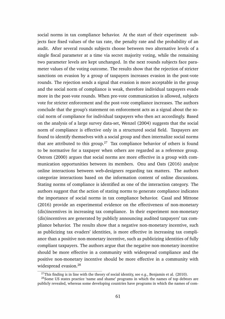
social norms in tax compliance behavior. At the start of their experiment sub-

jects face fixed values of the tax rate, the penalty rate and the probability of an

audit. After several rounds subjects choose between two alternative levels of a

single fiscal parameter at a time via secret majority voting, while the remaining

two parameter levels are kept unchanged. In the next rounds subjects face para-

meter values of the voting outcome. The results show that the rejection of stricter

sanctions on evasion by a group of taxpayers increases evasion in the post-vote

rounds. The rejection sends a signal that evasion is more acceptable in the group

and the social norm of compliance is weak, therefore individual taxpayers evade

more in the post-vote rounds. When pre-vote communication is allowed, subjects

vote for stricter enforcement and the post-vote compliance increases. The authors

conclude that the group’s statement on enforcement acts as a signal about the so-

cial norm of compliance for individual taxpayers who then act accordingly. Based

on the analysis of a large survey data-set, Wenzel (2004) suggests that the social

norm of compliance is effective only in a structured social field. Taxpayers are

found to identify themselves with a social group and then internalize social norms

that are attributed to this group.27 Tax compliance behavior of others is found

to be normative for a taxpayer when others are regarded as a reference group.

Ostrom (2000) argues that social norms are more effective in a group with com-

munication opportunities between its members. Onu and Oats (2016) analyze

online interactions between web-designers regarding tax matters. The authors

categorize interactions based on the information content of online discussions.

Stating norms of compliance is identified as one of the interaction category. The

authors suggest that the action of stating norms to generate compliance indicates

the importance of social norms in tax compliance behavior. Casal and Mittone

(2016) provide an experimental evidence on the effectiveness of non-monetary

(dis)incentives in increasing tax compliance. In their experiment non-monetary

(dis)incentives are generated by publicly announcing audited taxpayers’ tax com-

pliance behavior. The results show that a negative non-monetary incentive, such

as publicizing tax evaders’ identities, is more effective in increasing tax compli-

ance than a positive non-monetary incentive, such as publicizing identities of fully

compliant taxpayers. The authors argue that the negative non-monetary incentive

should be more effective in a community with widespread compliance and the

positive non-monetary incentive should be more effective in a community with

widespread evasion.28

27This finding is in line with the theory of social identity, see e.g., Benjamin et al. (2010).28Some US states practice ‘name and shame’ programs in which the names of top debtors are

publicly revealed, whereas some developing countries have programs in which the names of com-

61

The traditional models’ failure in explaining empirically observed levels of com-

pliance has motivated theorists to consider non-monetary incentives as additional

factors of compliance. The analysis has been extended within EU framework by

allowing an additive preference structure of the following form:

U(D,W, t, p, λ) = E[u(D,W, t, p, λ)] + S([W −D], n) (1.1)

where E[u(·)] represents expected utility of an evasion lottery, when a taxpayer

with the income level W reports the amount D for given levels of the tax rate, t,

the penalty rate, λ, and the probability of an audit, p. Non-monetary incentives for

compliance are captured by the term S(·), that is a function of one’s own evaded

income [W − D] and the share of evaders in the society, n. For example, Gordon

(1989) considers the following linear functional form of S(·):

S([W −D], n) = −[W −D][a+ b[1− n]] (1.2)

where a > 0 is an individual-specific marginal ‘private stigma’ from evasion and

b[1 − n], with another individual-specific parameter b > 0, is referred to as the

marginal ‘social stigma’ from evasion. A taxpayer who evades the amount of in-

come [W − D] suffers total private stigma of a[W − D] and the social stigma of

b[1− n][W −D], that is decreasing in the fraction of evaders in the society, n.

Traxler (2010) suggests a more general functional form of S(·), that captures

non-monetary incentives for compliance:

S([W −D], n) = −δ[W −D]f(n) (1.3)

where δ > 0 is an individual-specific ‘degree of norm internalization’ and the

continuous function f(n) captures the strength of the social norm of compliance

in the society. f(·) is assumed to have the following properties, 0 < f(n) <∞ and

f ′(n) ≤ 0 for n ∈ [0, 1]. Therefore, if the fraction of evaders is high, the social norm

of compliance is weak and the marginal non-monetary cost of evasion is low for a

taxpayer.

A similar approach is taken by Myles and Naylor (1996), who analyze a social

custom of compliance, assuming that a fully compliant taxpayer derives strictly

positive conformity payoff that is decreasing in the fraction of evaders in the soci-

ety. If a taxpayer evades some income, he gets zero conformity payoff.

The literature that analyzes the interplay between economic incentives and so-

pliant taxpayers are publicized (Luttmer and Singhal, 2014).

62

cial norms in the context of tax compliance (e.g., Gordon, 1989 and Traxler, 2010),

can explain why some people never evade taxes. Such models predict higher com-

pliance levels than the models that consider economic incentives only. Yet, there

are several challenges these models fail to address. First, it is only the fraction of

evaders, not the magnitude or extent of evasion, that signals the strength of the

social norm of compliance in these models. For instance, if in one case fraction n of

taxpayers evades half of their income (fraction [1−n] being fully compliant) and in

another case, the same fraction n evades all their income, nevertheless the strength

of social norms would be identical in the two cases. Therefore, the model should

consider not only the fraction of evaders, but also the volume or extent of evasion

as a measure for the strength of the social norm of compliance. Second, existing

models either consider only social stigma and guilt from non-compliance with the

norm (e.g.,Traxler, 2010) or conformity payoff from compliance with the norm

(e.g., Myles and Naylor, 1996), whereas evidence shows that guilt and esteem

are both important components of compliance behavior (e.g., Casal and Mittone,

2016). Lastly, virtually all the tax compliance models using EU fail to correctly

predict the tax rate-compliance relation. Empirical evidence shows that evasion

increases in the tax rate (e.g. Clotfelter, 1983; Pudney et al., 2000), whereas

theoretical models using EU either predict the inverse (e.g., Yitzhaki, 1974) or

ambiguous relationship between compliance and the tax rate (See Andreoni et al.,

1998; Sandmo, 2005 and Slemrod, 2007 for surveys).

This chapter suggests an alternative theoretical approach to the social norm

of compliance and develops a model of tax compliance using prospect theory of

Kahneman and Tversky (1979) and Tversky and Kahneman (1992). To the best of

my knowledge, this is the first work that formalizes the social norm of compliance

in the prospect theory framework. 29 The model builds upon the following main

assumptions:

1. A taxpayer internalizes norm of compliance that is attributed to his reference

income group (consistent with Wenzel, 2004).

2. A taxpayer cares about his performance relative to the average compliance

level in his reference income group. Falling below the average declaration

induces guilt that exceeds, in absolute value, esteem derived from higher in-

come declaration of the equivalent magnitude relative to the average (con-

sistent with Casal and Mittone, 2016).29Alm and Torgler (2011) discuss the relevance of prospect theory and argue that social norms

might affect a taxpayer’s reference point. Cullis et al. (2012) informally discuss the importance ofprospect theory in explaining the effects of social norm on compliance.

63

3. A taxpayer treats his legal after-tax income as a reference point for eco-

nomic outcomes (Dhami and al-Nowaihi, 2007) and regards the average

compliance of his reference income-group as a reference point for societal

outcomes.

4. Taxpayers have heterogeneous preferences in the sense that the relative

weight given to the economic and the societal outcomes may differ for each

taxpayer.

By considering a continuum of heterogeneous taxpayers, the model enables

us to endogenously derive the equilibrium level of the average group compliance

and the related strength of the social norm. Consistent with evidence, the model

suggests that the equilibrium level of an average group compliance decreases in

the tax rate and increases in the tax enforcement parameters - the penalty rate and

the probability of an audit. Therefore, ceteris paribus, an increase in the tax rate

weakens the norm of compliance, whereas the norm is stronger under the stricter

tax enforcement regime.

The rest of the chapter is structured as follows. Section 2 presents the model.

Section 3 considers the compliance problem of an individual taxpayer. Section 4

derives the equilibrium group behavior with heterogeneous taxpayers and Section

5 concludes.

2 The Model

An individual has exogenously given income level W, that is subject to tax. The flat

tax rate t ∈ (0, 1) is levied on the declared income D ∈ [0,W ]. The tax authority

carries out random income audits, and if the taxpayer is caught underreporting

his income, he has to pay the evaded taxes and a penalty. The probability of an

audit, p ∈ (0, 1), is assumed to be exogenously given to the taxpayer and it is

independent of the declared income. If the taxpayer is not audited, his after-tax

income is given by the following:

YNA = W − tD (2.1)

and in case of an audit, the disposable income of the taxpayer is:

YA = [1− t]W − λt[W −D] (2.2)

64

where λ > 0 denotes the penalty rate and λt[W − D] is the total penalty that is

proportional to the evaded taxes.

A taxpayer’s preferences over the monetary and social outcomes are given by

the following form:

U(Y,R,D, DbW , β) = [1− β]v(Y −R) + βu(D − Db

W ) (2.3)

The explanation of (2.3) is as follows. v(·) is the prospect theory value function

defined over the difference between the after-tax income, Y, and the reference in-

come level, R. Monetary (dis)incentives for compliance are captured by v(·) in the

model. u(·) is another value function that embodies the taxpayer’s societal incen-

tives for compliance. The argument of u(·) is the difference between the taxpayer’s

declared income, D, and his belief about the average declaration in his reference

income group, DbW . The parameter 0 ≤ β ≤ 1 captures the relative importance of

societal outcomes in the preferences. For the sake of clear exposition, the value

functions are assumed to be piecewise linear. The value function embodying mon-

etary (dis)incentives for compliance is given by the following:

v(x) =

x, if x ≥ 0

θx, if x < 0(2.4)

where x is income relative to the reference income level. When x ≥ 0, an individ-

ual is in the domain of gains, otherwise he is in the domain of losses. θ > 1 is the

loss aversion parameter, manifesting that the absolute value of disutility from loss

is greater than utility from the equivalent gain.

The value function embodying societal incentives for compliance has the fol-

lowing form:

u(d) =

d, if d ≥ 0

γd, if d < 0(2.5)

where d is the difference between a taxpayer’s own declared income, D, and his

perception of the average declaration in the reference income group, DbW . The

taxpayer experiences esteem if he declares higher income than his belief about the

average declaration in his income group and suffers guilt if he falls below his belief

about the average. γ > 1 is the guilt aversion parameter. Hence, falling below the

average declaration induces sensation of guilt that exceeds, in absolute value, es-

teem derived from higher income declaration of the equivalent magnitude relative

to the average. The guilt aversion formulation in the context of tax compliance is

consistent with the recent experimental evidence. Casal and Mittone (2016) find

65

that a negative non-monetary incentive, such as publicizing tax evaders’ identi-

ties, is more effective in increasing tax compliance than a positive non-monetary

incentive, such as publicizing identities of fully compliant taxpayers. In light of a

continuum of taxpayers, as it is specified below, on margin a taxpayer’s declaration

decision does not affect other taxpayers’ utilities, therefore this paper abstracts

from the psychological game theoretic considerations of guilt.30

The suggested formulation of preferences captures the essence of the social

norm of compliance. Consistent with empirical evidence (e.g., Wenzel, 2004), the

social norm of compliance is effective if an individual identifies himself with a ref-

erence group to which the norm is attributed. Once identified, the positive effect

of the social norm is mediated by internalization of the norm. Wenzel (2004) sug-

gests that "people could consider their occupational group or their income group

to be more important in the area of tax." Alm et al. (1999) write: "The stronger

is the social norm, the more deviant the behavior of a non-compliant individual

becomes, and the more loss the individual feels" (page 149). In line with these in-

sights, higher is the average compliance in the reference income group and hence,

beliefs about this average, DbW , greater is the societal incentive to revise one’s own

declaration. Conversely, stronger is the social norm of compliance in the income

group, ceteris paribus, lower is the overall evasion and thus, higher is the average

declaration in the given group. The importance of the norm in individual com-

pliance behavior is determined by the following two factors. First, exogenously

given individual-specific parameter, β, that can be interpreted as the degree of

norm internalization. Second, one’s belief about the average income declaration

in his income group.

It is assumed that a taxpayer’s reference income is equal to his legal-after tax

income (status-quo). Hence:

R = [1− t]W (2.6)

The specification of the reference income in (2.6) is adopted from Dhami and al-

Nowaihi (2007), who advocate the legal after-tax income as a reference income

level in the prospect theory framework. The authors show that for all declaration

levels, D ∈ [0,W ] , a non-audited taxpayer is in the domain of gains and an audited

taxpayer is in the domain of losses if and only if the legal after-tax income is the

reference point, i.e., R = [1− t]W. Adherence to this specification of the reference

30In psychological game theoretic models an individual’s utility depends, not only on monetarypayoffs from actions, but also on his beliefs about other individual’s actions (first order belief) andon his beliefs about other individual’s beliefs (second order belief). An individual may experienceguilt if he lets another player down, based on her second order belief. See e.g., Battigalli andDufwenberg (2007, 2009) for modelling guilt in psychological game theoretic framework.

66

income is of decisive importance to predict the empirically correct compliance-tax

rate relation.

A taxpayer, who considers underreporting his income because of pure mone-

tary incentives, cares about the position of his after-tax income relative to the ref-

erence point. Using (2.1), (2.2), (2.6) and recalling that D ∈ [0,W ], the after-tax

income of a non-audited taxpayer and the after-tax income of an audited taxpayer

relative to the reference point are given by (2.7) and (2.8), respectively:

xna = t[W −D] ≥ 0 (2.7)

xa = −λt[W −D] ≤ 0 (2.8)

Consistent with empirical evidence (e.g., Kahneman and Tversky, 1979; Tver-

sky and Kahneman, 1992), a taxpayer overweights low probabilities and under-

weights high probabilities. Using a probability weighting function ω(·), that is

continuous and strictly increasing function from [0, 1] onto [0, 1] with ω(0) = 0 and

ω(1) = 1, the weights given to the audit and non-audit probabilities are ω(p) and

ω(1− p), respectively.31

The model is closed by considering a continuum of taxpayers, with heteroge-

neous pretax income levels and individual-specific parameter values, β. Taxpayers

are located on the unit square Ω(β, z) = [0, 1]× [0.1] , where z is a locational label

of an individual taxpayer. Pretax income is given by the density function W (z).

Apart from the parameter tuple (β, z), taxpayers are identical. The loss aversion

parameter, θ, and the guilt aversion parameter, γ, are the same for all individuals

and the preferences of each taxpayer are represented by (2.3).

3 The Taxpayer’s Compliance Problem

Consider a taxpayer who is located at the point (β, z) of the unit square Ω. Given

his income level, W (z), parameter values of p, t, λ, β and the probability weighting

function ω(·), the taxpayer chooses the optimal amount of income to declare, D.

Using (2.3), the taxpayer maximizes the following:

V = [1− β] ω(p)v(YA −R) + ω(1− p)v(YNA −R)+ βu(D − DbW ) (3.1)

31Here it is assumed that the probability weighting function for losses is the same as the one forgains, which need not be true in general.

67

From (2.1), (2.2), (2.6) and (3.1) we get:

V = [1− β] ω(p)v(xa) + ω(1− p)v(xna)+ βu(D − DbW ) (3.2)

where xna ≥ 0 and xa ≤ 0 are given by (2.7) and (2.8), respectively.

The taxpayer’s preferences consist of two domains - economic and social, which

bear respective weights of [1 − β] and β. The taxpayer is under the risk of audit,

if he evades taxes. If the evasion gets detected, the taxpayer is in the domain of

losses, xa ≤ 0, otherwise, he is in the domain of gains, xna ≥ 0. The decision

weights of ω(p) and ω(1 − p) are assigned to the audit and non-audit outcomes,

respectively.32 Hence, monetary (dis)incentives for compliance are captured by

the term ω(p)v(xa) + ω(1− p)v(xna) . Societal incentives for compliance are cap-

tured by the value function u(D − DbW ). In the social domain, the taxpayer com-

pares his own declared amount, D, with his belief about the average declaration

in his income group.

From (2.4), (2.7), (2.8) and (3.2) we obtain:

V = [1− β] −ω(p)θλt[W −D] + ω(1− p)t[W −D]+ βu(D − DbW ) (3.3)

Rearranging (3.3) results in:

V = [1− β]× t[W −D] ω(1− p)− ω(p)θλ+ βu(D − DbW ) (3.4)

Let I = ω(1− p)− ω(p)θλ . Note that the value of I decreases in the tax

enforcement parameters, p (because ω(·) is strictly increasing function) and λ.

Therefore, stronger is the tax enforcement because of higher probability of an

audit or higher penalty rate, lower is I. Hence, I represents the strength of the tax

enforcement regime. (3.4) can be rewritten as:

V = [1− β]× t[W −D]I + βu(D − DbW ) (3.5)

Note that, if I ≤ 0, the taxpayer optimally declares all his income, W, ∀β ∈ [0, 1].

Assuming I > 0, 33 the taxpayer declares the amount of income D ∈ [0,W ], that

maximizes (3.5).

Proposition 3.1 Suppose I > 0. Then a taxpayer optimally declares D∗ = 0 if β <32For a two-outcome lottery, decision weights coincide with probability weights.33For the realistic parameter values, 0 < I < 1. E.g., for the following parameter values, taken

from Dhami and al-Nowaihi (2007), p = 0.03, θ = 2.25, λ = 1 and the probability weightingfunction ω(p) = e−(− ln p)

0.5

, I ≈ 0.49.

68

tIγ+tI

, D∗ = DbW if tI

γ+tI< β < tI

1+tIand D∗ = W if β > tI

1+tI

Proof. Firstly consider the case D ≥ DbW . Then, using (2.5) and (3.5) we get:

V = [1− β]× t[W −D]I + β[D − DbW ] (3.6)

Rearranging the right hand side of (3.6) gives:

V = D β − t[1− β]I+ t[1− β]WI − βDbW (3.7)

For D ≥ DbW , the expression in (3.7) achieves its maximum at D = Db

W if

β < tI1+tI

or at D = W if β > tI1+tI

.

Next consider the case D ≤ DbW . Then, using (2.5) and (3.5) we have:

V = [1− β]× t[W −D]I + βγ[D − DbW ] (3.8)

(3.8) can be written as:

V = D βγ − t[1− β]I+ t[1− β]WI − βγDbW (3.9)

For D ≤ DbW , the expression in (3.9) is maximized at D = 0 if β < tI

γ+tIor at

D = DbW if β > tI

γ+tI.

Given γ > 1, it follows that tIγ+tI

< tI1+tI

. For β < tIγ+tI

< tI1+tI

, it is optimal to

declare DbW under the first case, where D ≥ Db

W , but 0 under the second case,

where D ≤ DbW . Note that the option Db

W is also available in the second case, but

not optimal to choose. Hence, D∗ = 0 for β < tIγ+tI

< tI1+tI

.

For tIγ+tI

< β < tI1+tI

, it is optimal to declare DbW under the both cases, thus

D∗ = DbW .

And finally, for tIγ+tI

< tI1+tI

< β, we see that the optimal declaration amount

under the second case is available but not optimal to choose under the first case,

implying D∗ = W.

A taxpayer with sufficiently low degree of norm internalization, β < tIγ+tI

, de-

clares zero income and such behavior is driven by pure monetary incentives for

evasion. A taxpayer with high enough degree of norm internalization, β > tI1+tI

,

declares all income, W, and by doing so he avoids guilt if he believes that all the

taxpayers in his reference income group are honest, DbW = W, or derives esteem

if DbW < W . For the moderate values of β, the amount of declared income is

solely determined by a taxpayer’s belief about the average declaration in his in-

come group. In this case, the taxpayer ensures that he declares enough to avoid

69

guilt, D∗ = DbW . Hence, on an aggregate level there are three types of taxpayers

- unconditional evaders who neglect the social norm, unconditionally fully com-

pliant taxpayers who neglect monetary incentives for evasion and conditionally

compliant taxpayers who condition their compliance decision on the group aver-

age declaration. Therefore, the model is able to explain why some people never

evade taxes even in the existence of strong monetary incentives for evasion.

4 Equilibrium Group Compliance and Social Norms

Now we are able to investigate the equilibrium tax compliance behavior of an in-

come group of taxpayers. Beliefs of each taxpayer about the average reference

group compliance are required to be correct at the equilibrium, i.e., DbW = DW ,

where DW is the actual average declaration of the group. Recalling that the con-

tinuum of taxpayers are located on the unit square Ω(β, z), we have uniformly

distributed β−s in each income group, W (z). Then using Proposition 3.1 , beliefs

are correct if the following holds:

DW =

1∫0

D∗ dβ =

β2∫β1

DW dβ +

1∫β2

W dβ (4.1)

where, β1 = tIγ+tI

and β2 = tI1+tI

.

At the equilibrium, β1 share of the taxpayers with income level W declares zero

income; [β2 − β1] share of the taxpayers declares the average of the group, DW ,

and the remaining share, [1− β2], declares all income, W. From (4.1) Proposition

4.1 follows.

Proposition 4.1 There exists a unique equilibrium DbW = DW = 1−β2

β1+1−β2W, where

β1 = tIγ+tI

and β2 = tI1+tI

.34

Proof. From (4.1) we get:

DW = [β2 − β1]DW + [1− β2]W ⇒ (4.2)

DW =1− β2

β1 + 1− β2

W

34For the general case, where β−s are distributed according to the cumulative distribution func-tion F (β) over the [0, 1] interval, the equilibrium is Db

W = DW = 1−F (β2)1−F (β2)+F (β1)

W.

70

Note that the equilibrium value of the average declaration amount, DW , in-

creases in the share of fully compliant taxpayers in the group, [1 − β2], and de-

creases in the share of the taxpayers who evade all income, β1. Therefore, higher

is the share of fully compliant taxpayers in the group, stronger is the social norm of

compliance and higher is the share of the taxpayers who evade all income, weaker

is the social norm.

The compliance behavior of taxpayers is affected by the tax policy parame-

ters - the tax rate, t, the probability of an audit, p, and the penalty rate λ. The

equilibrium effects of these parameters are summarized in Proposition 4.2.

Proposition 4.2 Equilibrium value of the average group declaration, DW , strictlydecreases in the tax rate, t, but strictly increases in the probability of an audit, p, andthe penalty rate λ.

Proof. Substituting for β1 = tIγ+tI

and β2 = tI1+tI

in (4.2), we have:

DW =1

1+tI1

1+tI+ tI

γ+tI

W =1

1 + 1+tI1+ γ

tI

W (4.3)

Differentiation of (4.3) gives:

∂DW

∂t= −t

2I3 + 2γtI2 + γI

(t2I2 + 2tI + γ)2 W < 0 (4.4)

∂DW

∂I= −t

3I2 + 2γt2I + γt

(t2I2 + 2tI + γ)2 W < 0 (4.5)

From (4.4), (4.5) and recalling that I = ω(1− p)− ω(p)θλ is strictly decreas-

ing in the tax enforcement parameters, p and λ, the proposition directly follows.

Proposition 4.2 suggests that, ceteris paribus, higher is the tax rate, lower

is the average group compliance at the equilibrium. Therefore, an increase in

the tax rate weakens the social norm of compliance. The channel through which

the tax rate increase affects the equilibrium outcome is as follows. An increase

in the tax rate strengthens the monetary incentive for evasion. From (3.5), we

see that the economic return per unit of evaded income is equal to [1 − β] × tI,

that is larger for the higher tax rate, t. Therefore, the share of the taxpayers who

evade all income, β1 = tIγ+tI

, grows and the share of the fully compliant taxpayers,

[1 − β2] = 1 − tI1+tI

, diminishes. We also note that the share of the taxpayers,

71

[β2 − β1], who declare income in accordance to their beliefs about the average

declaration of the reference group, increases. The actual average declaration of

the group declines and the taxpayers update their beliefs accordingly, so that at the

new equilibrium with the higher tax rate the average amount of declared income

is lower.

The prediction, that an increase in the tax rate lowers the equilibrium amount

of the average group declaration, is in line with the evidence showing that evasion

increases in the tax rate (e.g., Clotfelter, 1983; Pudney et al., 2000). An increase

in the tax rate reduces the strength of the social norm of compliance. The senti-

ments expressed in the following quote from Lindbeck (1995) support this result.

"There must also be a price on honesty, in the sense that habits and social norms

that encourage such behavior may be undermined if honesty becomes sufficiently

expensive because of high marginal tax rates" (page 484).

An increase in the probability of an audit, p, or the penalty rate, λ, has a pos-

itive effect on the average group compliance at the equilibrium, that is in agree-

ment with intuition and evidence (see e.g., Slemrod, 2007). An increase in either

p or λ (or in both simultaneously), reduces I and therefore, reduces the economic

return per unit of evaded income, [1 − β] × tI. Lower share of taxpayers finds it

optimal to evade all income, i.e., the value of β1 = tIγ+tI

is smaller for smaller I.

Higher share of taxpayers declares all income, as the value of [1 − β2] is higher

for lower I. Those taxpayers who continue adhering to the social norm (and also

those, who switched their decision from zero income declaration) and declare the

amount they believe is the group average, adjust their beliefs upwards. As a result,

at the new equilibrium with stronger tax enforcement (lower I) the average group

compliance is higher.

The model predicts that the strength of the social norm of compliance in-

creases in the strength of the tax enforcement. The near-absolute enforcement

regime (high level of p or λ such that I → 0), ensures the full compliance of

each taxpayer, i.e., from (4.3) limI→0

DW = W, and establishes the absolute norm of

compliance. At another extreme, because of the taxpayers who neglect monetary

incentives and declare full income to derive the social esteem, the absence of the

tax enforcement does not induce social norm of zero compliance, i.e., from (4.3)

limI→1

DW = 11+ 1+t

1+γt

W > 0.

The social norm at the group level is linked with the norm at the aggregate

level. Integrating the right hand side of (4.3) using the distribution of income

72

W (z), we get:

D =

1∫0

1

1 + 1+tI1+ γ

tI

W dz =1

1 + 1+tI1+ γ

tI

W (4.6)

where D is the average social declaration and W is the average social income.

The strength of the social norm of compliance at the aggregate level has the

same determinants as the strength of the norm at the income group level. There-

fore, the tax authority aiming at increasing the norm of compliance, either has to

reduce the tax rate or stiffen the tax enforcement regime.

5 Concluding Remarks

The chapter suggests a way of modelling tax compliance behavior with endoge-

nous social norms in the prospect theory framework. The model rests on the

empirically supported assumptions that are new in the theoretical literature on so-

cial norms of compliance. First, in contrast to the existing models, it is the overall

extent of evasion and not only the share of evaders that signals the strength of the

social norm. Second, taxpayers identify themselves with a group of individuals

with the same income levels and internalize the norms that are attributed to this

group. Third, taxpayers are guilt averse in the social domain of their preferences.

The basic insight drawn from the model is that the tax policy parameters

not only shape monetary (dis)incentives for compliance, but also determine the

strength of the social norm of compliance at the equilibrium. Ceteris paribus, the

model predicts that an increase in the tax rate weakens the norm of compliance

and the social norm is stronger under the stricter tax enforcement regime. The

model explains why some people never evade taxes, it also makes the empirically

correct prediction of the tax rate effect on compliance.

The model considers exogenous distribution of individual-specific parameter

values β and assumes that changes in the tax policy parameters do not affect

the degree of norm internalization. Under more general set-up, this assumption

should be loosened by allowing adjustment process in the distribution of β−s, the

rationale being that the changed tax environment might affect the way individ-

uals think of their tax obligations and affect the degree of norm internalization,

at least in the long run. For instance, higher extrinsic incentives for compliance

induced by stricter tax enforcement may crowd out intrinsic incentives for com-

pliance (Luttmer and Singhal, 2014). Evolutionary game theoretic approach, e.g.,

gene-culture coevolution model of Gintis and Helbing (2015), is a promising chan-

73

nel to extend the analysis from the stationary distribution case into a dynamic,

evolutionary case. This possible extension is left for the future research.

74

References

[1] Abdellaoui, M., Bleichrodt, H., & Paraschiv, C. (2007) Loss aversion un-

der prospect theory: a parameter-free measurement. Management Science,

53(10), pp. 1659-1674.

[2] Abeler, J., Falk, A., Goette, L., & Huffman, D. (2011) Reference points and

effort provision. American Economic Review, 101(2), pp. 470-492.

[3] Allingham, M. G., & Sandmo, A. (1972) Income tax evasion: a theoretical

analysis. Journal of Public Economics, 1(3-4), pp. 323-338.

[4] Alm, J., McClelland, G. H., & Schulze, W. D. (1992) Why do people pay

taxes? Journal of Public Economics, 48(1), pp. 21-38.

[5] Alm, J., McClelland, G. H., & Schulze, W. D. (1999) Changing the social

norm of tax compliance by voting. KYKLOS, 52(2), pp. 141-171.

[6] Alm, J., & Torgler, B., (2011) Do ethics matter? Tax compliance and morality.

Journal of Business Ethics, 101(4), pp. 635-651.

[7] Alm, J. (2012) Measuring, explaining, and controlling tax evasion: lessons

from theory, experiments, and field studies. International Tax and Public Fi-

nance, 19(1), pp. 54-77.

[8] Andreoni, J., Erard, B., Feinstein, J. (1998) Tax compliance. Journal of Eco-

nomic Literature, 36(2), pp. 818-860.

[9] Arkes, H., Hirshleifer, D., Jiang, D., & Lim, S. (2008) Reference point adap-

tation: tests in the domain of security trading. Organizational Behavior and

Human Decision Processes, 105(1), pp. 67-81.

[10] Battigalli, P., & Dufwenberg, M. (2007) Guilt in games. American Economic

Review, 97(2), pp. 170-176.

[11] Battigalli, P., & Dufwenberg, M. (2009) Dynamic psychological games. Jour-

nal of Economic Theory, 144(1), pp. 1-35.

[12] Becker, G. S. (1968) Crime and punishment: an economic approach. Journal

of Political Economy, 76(2), pp. 169-217.

[13] Bell, D. E. (1982) Regret in decision making under uncertainty. Operations

Research, 30(5), pp. 961-981.

75

[14] Bell, D. E. (1985) Disappointment in decision making under uncertainty.

Operations Research, 33(1), pp. 1-27.

[15] Benjamin, D. J., Choi, J.J., & Strickland, A.J. (2010) Social identity and

preferences. American Economic Review, 100(4), pp. 1913-1928.

[16] Benjamini, Y., & Maital, S. (1985) Optimal tax evasion policy: behavioral

aspects, in Gaertner, W., & Wenig, A. (eds.), The economics of the shadow

economy, Berlin: Springer-Verlag, pp. 140-158.

[17] Bernasconi, M., & Zanardi, A. (2004) Tax evasion, tax rates and reference

dependence. FinanzArchiv, 60(3), pp. 422–445.

[18] Bernasconi, M., Corazzini, L., & Seri, R. (2014) Reference dependent pref-

erences, hedonic adaptation and tax evasion: does the tax burden matter?

Journal of Economic Psychology, 40, pp. 103-118.

[19] Casal, S., & Mittone, L. (2016) Social esteem versus social stigma: The role

of anonymity in an income reporting game. Journal of Economic Behavior

and Organization, 124, pp. 55-66.

[20] Clotfelter, C. T. (1983) Tax evasion and tax rates: an analysis of individual

returns. The Review of Economics and Statistics, 65(3), pp. 363-373.

[21] Crawford, V. P., & Meng, J. (2011) New York city cab drivers’ labor supply re-

visited: reference-dependent preferences with rational expectations targets

for hours and income. American Economic Review, 101(5), pp. 1912 -1932.

[22] Cullis, J. G., & Lewis, A. (1997) Why people pay taxes: From a conventional

economic model to a model of social convention. Journal of Economic Psy-

chology, 18(2-3), pp. 305-321.

[23] Cullis, J. G., Jones, P., & Savoia, A. (2012) Social norms and tax compliance:

Framing the decision to pay tax. Journal of Socio-Economics, 41(2), pp. 159-

168.

[24] Delquié, P., & Cillo, A. (2006) Expectations, disappointment, and rank-

dependent probability weighting. Theory and Decision, 60(2), pp. 193-206.

[25] Dhami, S., & al-Nowaihi, A. (2007) Why do people pay taxes? Prospect

theory versus expected utility theory. Journal of Economic Behavior and Or-

ganization, 64(1), pp. 171-192.

76

[26] Dhami, S., & al-Nowaihi, A. (2010) Optimal taxation in the presence of tax

evasion: expected utility versus prospect theory. Journal of Economic Behav-

ior and Organization, 75(2), pp. 313-337.

[27] Eide, E. (2001) Rank dependent expected utility models of tax evasion. Uni-

versity of Oslo, Mimeo.

[28] Elster, J. (1989) Social norms and economic theory. Journal of Economic

Perspectives, 3(4), pp. 99-117.

[29] Ericson, K. M. M., & Fuster, A. (2011) Expectations as endowments: evi-

dence on reference-dependent preferences from exchange and valuation ex-

periments. Quarterly Journal of Economics, 126(4), pp. 1879-1907.

[30] Frederick, S., & Loewenstein, G. (1999) Hedonic adaptation, in Kahneman,

D., Diener, E., & Schwarz, N. (eds.), Well-being: the foundations of hedonic

psychology, New York: Russell Sage Foundation, pp. 302–329.

[31] Friedland, N., Maital, S., & Rutenberg, A. (1978) A simulation study of in-

come tax evasion. Journal of Public Economics, 10(1), pp. 107-116.

[32] Gill, D., & Prowse, V. (2012) A structural analysis of disappointment aversion

in a real effort competition. American Economic Review, 102(1), pp. 469-

503.

[33] Gintis, H., & Helbing, D. (2015) Homo socialis: An analytical core for socio-

logical theory. Review of Behavioral Economics, 2(1-2), pp. 1-59.

[34] Gordon, J. P. F., (1989) Individual morality and reputation costs as deterrents

to tax evasion. European Economic Review, 33(4), pp. 797-805.

[35] Gul, F. (1991) A theory of disappointment aversion. Econometrica, 59(3),

pp. 667-686.

[36] Helson, H. (1947) Adaptation-level as frame of reference for prediction of

psychophysical data. American Journal of Psychology, 60(1), pp. 1-29.

[37] Helson, H. (1948) Adaptation-level as a basis for a quantitative theory of

frames of reference. Psychological Review, 55(6), pp. 297-313.

[38] Kahneman, D., & Tversky, A. (1979) Prospect theory: an analysis of decision

under risk. Econometrica, 47(2), pp. 263-291.

77

[39] Köszegi, B., & Rabin, M. (2006) A model of reference-dependent prefer-

ences. Quarterly Journal of Economics, 121(4), pp.1133-1165.

[40] Köszegi, B., & Rabin, M. (2007) Reference-dependent risk attitudes. Ameri-

can Economic Review, 97(4), pp. 1047-1073.

[41] Lindbeck, A. (1995) Welfare state disincentives with endogenous habits and

norms. Scandinavian Journal of Economics, 97(4), pp. 477-494.

[42] Loomes, G., & Sugden, R. (1982) Regret theory: an alternative theory of

rational choice under uncertainty. Economic Journal, 92(368), pp. 805-824.

[43] Loomes, G., & Sugden, R. (1986) Disappointment and dynamic consistency

in choice under uncertainty. Review of Economic Studies, 53(2), pp. 271-

282.

[44] Luttmer, E. F. P., & Singhal, M. (2014) Tax morale. Journal of Economic Per-

spectives, 28(4), pp. 149-168.

[45] Lyubomirsky, S. (2011) Hedonic adaptation to positive and negative experi-

ences, in Folkman, S. (ed.), Oxford handbook of stress, health, and coping,

New York: Oxford University Press, pp. 200-224.

[46] March, J.G. (1988) Variable risk preferences and adaptive aspirations. Jour-

nal of Economic Behavior and Organization, 9(1), pp. 5-24.

[47] Myles, G. D., & Naylor, R. A. (1996) A model of tax evasion with group con-

formity and social customs. European Journal of Political Economy, 12(1),

pp. 49-66.

[48] Onu, D., & Oats, L. (2016) "Paying tax is part of life”: Social norms and

social influence in tax communications. Journal of Economic Behavior and

Organization, 124, pp. 29-42.

[49] Ostrom, E. (2000) Collective action and the evolution of social norms. Jour-

nal of Economic Perspectives, 14(3), pp. 137-158.

[50] Posner R. A., & Rasmusen E. B. (1999) Creating and enforcing norms, with

special reference to sanctions. International Review of Law and Economics,

19(3), pp. 369-382.

[51] Pudney, S. E., Pyle, D., & Saruc, T. (2000) Income tax evasion: an exper-

imental approach, in MacDonald, Z., & Pyle, D. (eds.), Illicit activity: the

economics of crime, drugs and tax fraud, Aldershot: Ashgate, pp. 267-289.

78

[52] Quiggin, J. (1982) A theory of anticipated utility. Journal of Economic Be-

havior and Organization, 3(4), pp. 323-343.

[53] Quiggin, J. (1993) Generalized expected utility theory: the rank-dependent

model, Boston: Kluwer Academic Publishers.

[54] Sandmo, A. (2005) The theory of tax evasion: a retrospective view. National

Tax Journal, 58(4), pp. 643-663.

[55] Siegel, S., Hinson, R. E., Krank, M. D., & McCully, J. (1982) Heroin "over-

dose" death: contribution of drug-associated environmental cues. Science,

216(4544), pp. 436-437.

[56] Slemrod, J. (2007) Cheating ourselves: the economics of tax evasion. Jour-

nal of Economic Perspectives, 21(1), pp. 25-48.

[57] Traxler, C. (2010) Social norms and conditional cooperative taxpayers. Eu-

ropean Journal of Political Economy, 26(1), pp. 89-103.

[58] Tversky, A., Kahneman, D. (1992) Advances in prospect theory: cumulative

representation of uncertainty. Journal of Risk and Uncertainty, 5(4), pp. 297-

323.

[59] van Praag, B. (1971) The welfare function of income in Belgium: an empiri-

cal investigation. European Economic Review, 2(3), pp. 337-369.

[60] van Praag, B. M. S., & van der Sar, N. L. (1988) Empirical uses of subjective

measures of well-being. Journal of Human Resources, 23(2), pp. 193-210.

[61] Wenzel, M. (2004) An analysis of norm processes in tax compliance. Journal

of Economic Psychology, 25(2), pp. 213-228.

[62] Yaniv, G. (1999) Tax compliance and advance tax payments: a prospect the-

ory analysis. National Tax Journal, 52(4), pp. 753-764.

[63] Yitzhaki, S. (1974) A note on "income tax evasion: a theoretical analysis".

Journal of Public Economics, 3(2), pp. 201-202.

79