Embed Size (px)
Citation preview
Tait colorings, and an instanton homology forwebs and foams
P. B. Kronheimer and T. S. Mrowka
Harvard University, Cambridge MA 02138Massachusetts Institute of Technology, Cambridge MA 02139
Abstract. We use SO(3) gauge theory to define a functor from a category of unorientedwebs and foams to the category of finite-dimensional vector spaces over the field of twoelements. We prove a non-vanishing theorem for this SO(3) instanton homology of webs,using Gabai’s sutured manifold theory. It is hoped that the non-vanishing theorem maysupport a program to provide a new proof of the four-color theorem.
The work of the first author was supported by the National Science Foundation through NSFgrants DMS-0904589 and DMS-1405652. The work of the second author was supported by NSFgrants DMS-0805841 and DMS-1406348.
arX
iv:1
508.
0720
5v1
[m
ath.
GT
] 2
8 A
ug 2
015
2
Contents
1 Introduction 41.1 Statement of results . . . . . . . . . . . . . . . . . . . . . . . . . . . . 41.2 Functoriality . . . . . . . . . . . . . . . . . . . . . . . . . . . . . . . . 51.3 Remarks about the proof of Theorem 1.1 . . . . . . . . . . . . . . . . . 61.4 Outline of the paper . . . . . . . . . . . . . . . . . . . . . . . . . . . . 7
2 Preliminaries 72.1 Orbifolds . . . . . . . . . . . . . . . . . . . . . . . . . . . . . . . . . . 72.2 Bifolds from embedded webs and foams . . . . . . . . . . . . . . . . . 82.3 Orbifold connections . . . . . . . . . . . . . . . . . . . . . . . . . . . . 92.4 Marked connections . . . . . . . . . . . . . . . . . . . . . . . . . . . . 102.5 ASD connections and the index formula . . . . . . . . . . . . . . . . . . 122.6 Bubbling . . . . . . . . . . . . . . . . . . . . . . . . . . . . . . . . . . 152.7 The Chern-Simons functional . . . . . . . . . . . . . . . . . . . . . . . 182.8 Representation varieties . . . . . . . . . . . . . . . . . . . . . . . . . . 192.9 Examples of representation varieties . . . . . . . . . . . . . . . . . . . . 21
3 Construction of the functor J 233.1 Discussion . . . . . . . . . . . . . . . . . . . . . . . . . . . . . . . . . 233.2 Holonomy perturbations . . . . . . . . . . . . . . . . . . . . . . . . . . 243.3 Proof that d2 = 0 mod 2 . . . . . . . . . . . . . . . . . . . . . . . . . . 263.4 Functoriality of J . . . . . . . . . . . . . . . . . . . . . . . . . . . . . . 313.5 Foams with dots . . . . . . . . . . . . . . . . . . . . . . . . . . . . . . 343.6 Defining J] . . . . . . . . . . . . . . . . . . . . . . . . . . . . . . . . . 383.7 Simplest calculations . . . . . . . . . . . . . . . . . . . . . . . . . . . . 40
4 Excision 404.1 Floer’s excision argument . . . . . . . . . . . . . . . . . . . . . . . . . 404.2 Applications of excision . . . . . . . . . . . . . . . . . . . . . . . . . . 42
5 Calculations 445.1 The unknot and the sphere with dots . . . . . . . . . . . . . . . . . . . . 445.2 The theta foam and the theta web . . . . . . . . . . . . . . . . . . . . . 465.3 The tetrahedron web and its suspension . . . . . . . . . . . . . . . . . . 475.4 Upper bounds for some prisms . . . . . . . . . . . . . . . . . . . . . . . 49
6 Relations 506.1 The neck-cutting relation . . . . . . . . . . . . . . . . . . . . . . . . . . 506.2 The bigon relation . . . . . . . . . . . . . . . . . . . . . . . . . . . . . 526.3 The triangle relation . . . . . . . . . . . . . . . . . . . . . . . . . . . . 546.4 The square relation . . . . . . . . . . . . . . . . . . . . . . . . . . . . . 576.5 Simple graphs . . . . . . . . . . . . . . . . . . . . . . . . . . . . . . . 58
3
7 Proof of non-vanishing, Theorem 1.1 587.1 Passing from J] to I] . . . . . . . . . . . . . . . . . . . . . . . . . . . . 587.2 Removing vertices . . . . . . . . . . . . . . . . . . . . . . . . . . . . . 607.3 A taut sutured manifold . . . . . . . . . . . . . . . . . . . . . . . . . . 627.4 Proof of tautness . . . . . . . . . . . . . . . . . . . . . . . . . . . . . . 65
8 Tait-colorings, O(2) representations and other topics 678.1 O(2) connections and Tait colorings of spatial and planar graphs . . . . . 678.2 Foams with non-zero evaluation, and O(2) connections . . . . . . . . . . 688.3 A combinatorial counterpart . . . . . . . . . . . . . . . . . . . . . . . . 718.4 Gradings . . . . . . . . . . . . . . . . . . . . . . . . . . . . . . . . . . 738.5 The relation between I] and J] . . . . . . . . . . . . . . . . . . . . . . . 758.6 Replacing SO(3) by SU(3) . . . . . . . . . . . . . . . . . . . . . . . . . 80
4
1 Introduction
1.1 Statement of results
By a web in R3 we shall mean an embedded trivalent graph. More specifically, aweb will be a compact subset K ⊂ R3 with a finite set V of distinguished points,the vertices, such that K\V is a smooth 1-dimensional submanifold of R3, andsuch that each vertex has a neighborhood in which K is diffeomorphic to threedistinct, coplanar rays in R3. We shall refer to the components of K\V as theedges. Note that our definition allows an edge to be a (possibly knotted) circle.The vertex set may be empty.
An edge e of K is an embedded bridge if there is a smoothly embedded 2-sphere in R3 which meets e transversely in a single point and is otherwise disjointfrom K. We use the term “embedded bridge” to distinguish this from the moregeneral notion of a bridge, which is an edge whose removal increases the numberof connected components of K.
A Tait coloring of K is a function from the edges of K to a 3-element setof “colors” { 1, 2, 3 } such that edges of three different colors are incident at eachvertex. Tait colorings which differ only by a permutation of the colors will still beregarded as distinct; so if K is a single circle, for example, then it has three Taitcolorings.
In this paper, we will show how to associate a finite-dimensional F-vectorspace J](K) to any web K in R3, using a variant of the instanton homology forknots from [5] and [15], but with gauge group SO(3) replacing the group SU(2)as it appeared in [15]. (Here F is the field of 2 elements.) We will establish thefollowing non-vanishing property for J].
Theorem 1.1. For a web K ⊂ R3, the vector space J](K) is zero if and only if Khas an embedded bridge.
Based on the evidence of small examples, and some general properties of J],we also make the following conjecture:
Conjecture 1.2. If the web K lies in the plane, so K ⊂ R2 ⊂ R3, then the dimen-sion of J](K) is equal to the number of Tait colorings of K.
The conjecture is true for planar webs which are bipartite. Slightly more gen-erally, we know that a minimal counterexample cannot contain any squares, tri-angles, bigons or circles. If the conjecture is true in general, then, together withthe preceding theorem, it would establish that every bridgeless, planar trivalent
5
graph admits a Tait coloring. The existence of Tait colorings for bridgeless triva-lent graphs in the plane is equivalent to the four-color theorem (see [22]), so theabove conjecture would provide an alternative proof of the theorem of Appel andHaken [1]: every planar graph admits a four-coloring.
1.2 Functoriality
The terminology of graphs as ‘webs’ goes back to Kuperberg [16] and was usedby Khovanov in [7], where Khovanov’s sl3 homology, F(K), was defined for ori-ented, bipartite webs K. The results of [7] have motivated a lot of the construc-tions in this paper, but our webs are more general, being unoriented and withoutthe bipartite restriction. At least for planar webs, one can repeat Khovanov’s com-binatorial definitions without the bipartite condition, but only by passing to F co-efficients. (We will take this up briefly in section 8.3.) In this way one can sketcha possible combinatorial counterpart to J](K), though it is not clear to the authorshow to calculate it, or even that this combinatorial version is finite-dimensional ingeneral.
A key property of J](K) is its functoriality for certain singular cobordismsbetween webs. Following [7], these singular cobordisms will be called foams,though the foams that are appropriate here are more general than those of [7], inline with our more general webs (see also [17]). A (closed) foam Σ in R4 will bea compact 2-dimensional subcomplex decorated with “dots”. The subcomplex isrequired to have one of the following models at each point x ∈ Σ:
(a) a smoothly embedded 2-manifold in a neighborhood of x;
(b) a neighborhood modeled on R × K3 where K3 ⊂ R3 is the union of three
distinct rays meeting at the origin; or
(c) a cone in R3 ⊂ R4 whose vertex is x and whose base is the union of 4 distinctpoints in S 2 joined pairwise by 6 non-intersecting great-circle arcs, each oflength at most π.
Points of the third type will be called tetrahedral points, because a neighbor-hood has the combinatorics of a cone on the 1-skeleton of a tetrahedron. (Singularpoints of this type appear in the foams of [17].) The points of the second type forma union of arcs called the seams. The seams and tetrahedral points together forman embedded graph in R4 whose vertices have valence 4. The complement of thetetrahedral points and seams is a smoothly embedded 2-manifold whose compo-nents are the facets of the foam. Each facet is decorated with a number of dots:
6
a possibly empty collection of marked points. No orientability is required of thefacets of Σ.
Given webs K and K′ in R3, we can also consider foams with boundary,Σ ⊂ [a, b]×R3, modeled on [a, a+ ε)×K at one end and (b− ε, b]×K′ at the other.The seams and tetrahedral points comprise a graph with interior vertices of va-lence 4 and vertices of valence 1 at the boundary. are either circles or arcs whoseendpoints lie on the boundary. We will refer to such a Σ as a (foam)-cobordismfrom K to K′. A cobordism gives rise to linear map,
J](Σ) : J](K)→ J](K′).
Cobordisms can be composed in the obvious way, and composite cobordisms giverise to composite maps, so we can regard J] as a functor from a suitable categoryof webs and foams to the category of vector spaces over F.
1.3 Remarks about the proof of Theorem 1.1
Theorem 1.1 belongs to the same family as other non-vanishing theorems for in-stanton homology proved by the authors in [13] and [15]. As with the earlierresults, the proof rests on the Gabai’s existence theorem for sutured manifold hi-erarchies, for taut sutured manifolds [6].
Given a web K ⊂ R3, let us remove a small open ball around each of the ver-tices, to obtain a manifold with boundary, each boundary component being spherewith 3 marked points. Now identify these boundary components in pairs (thenumber of vertices in a web is always even) to obtain a link K+ in the connectedsum of R3 with a number of copies of S 1 × S 2. Add a point at infinity to replaceR3 by S 3. Let M be the complement of a tubular neighborhood of K+. Form asutured manifold (M, γ) by putting two meridional sutures on each of the torusboundary components of M. By a sequence of applications of an excision princi-ple, we will show that the non-vanishing of J](K) is implied by the non-vanishingof the sutured instanton homology, SHI(M, γ), as defined in [13]. Furthermore,SHI(M, γ) will be non-zero provided that (M, γ) is a taut sutured manifold in thesense of [6]. Finally, by an elementary topological argument, we show that thetautness of (M, γ) is equivalent to the conditions that K ⊂ R3 is not split (i.e.admits no separating embedded 2-sphere) and has no embedded bridge. This es-tablishes Theorem 1.1 for the case of non-split webs, which is sufficient becauseof a multiplicative property of J] for split unions.
7
1.4 Outline of the paper
Section 2 deals with the gauge theory that is used in the definition of J]. Section 3defines the functor J] and establishes its basic properties. We define J] moregenerally than in this introduction, considering webs in arbitrary 3-manifolds. Insection 6, we establish properties of J] that are sufficient to calculate J](K) atleast when K is a bipartite planar graph, as well as some other simple cases. Thearguments in section 6 depend on applications of an excision principle which isdiscussed in section 4. The proof of Theorem 1.1 is given in section 7. Somefurther questions are discussed in section 8.
Acknowledgement. The authors are very grateful for the support of the RadcliffeInstitute for Advanced Study, which provided them with the opportunity to pursuethis project together as Fellows of the Institute during the academic year 2013–2014.
2 Preliminaries
2.1 Orbifolds
We will consider 3- and 4-dimensional orbifolds with the following local models.In dimension 3, we require that every singular point of the orbifold has a neigh-borhood which is modeled either on R × (R2/{±1}) or on R3/V4, where V4 is astandard Klein 4-group in SO(3). In the first of these cases, the singular set islocally a smooth 1-manifold, and in the second case the singular set is three half-lines meeting at a single vertex. In dimension 4, we allow local models which areeither products of one of the above two 3-dimensional models with R, or one addi-tional case, the quotient of R4 by the group V8 ⊂ SO(4) consisting of all diagonalmatrices with entries ±1 and determinant 1.
Every point in such an orbifold has a neighborhood U which is the codomainof an orbifold chart,
φ : U → U.
The map φ is a quotient map for an action of a group H which is either trivial, F,V4 or V8. If x is a point in U and x a preimage point, we write Hx for the stabilizerof x.
We introduce a term for this restricted class of orbifolds:
8
Definition 2.1. A bifold will mean a 3- or 4-dimensional orbifold whose localmodels belong to one of the particular types described above.
Our bifolds will be equipped with an orbifold Riemannian metric, which wecan regard as a smooth metric g on the complement of the singular set with theproperty that the pull-back of g via any orbifold chart φ extends to a smooth metricon the domain U of φ. In the 3-dimensional case, the singular set is an embeddedweb and the total space of the bifold is topologically a manifold. The Riemannianmetric will have cone-angle π along each edge of the graph. In the 4-dimensionalcase, the singular set is an embedded 2-dimensional complex Σ with the samecombinatorial structure as a foam, and cone-angle π along the facets of Σ.
2.2 Bifolds from embedded webs and foams
Given a smooth Riemannian 3-manifold Y containing a web K, smoothly embed-ded in the sense described in the introduction, we can construct a Riemannianbifold Y with a copy of K as its singular set by modifying the Riemannian met-ric in a neighborhood of K to introduce the required cone angles. To do this, wefirst adjust K so that, at each vertex the incident edges arrive with tangent direc-tions which are coplanar and at equal angles 2π/3. This can be done in a standardway, because the space of triples of distinct points in S 2 deformation-retracts tothe subspace of planar equilateral triangles. Once this is done, the neighborhoodsof the vertices are standard and we can use the smooth Riemannian metric g onY to introduce coordinates in which to modify the Riemannian metric, making itisometric to R3/V4 in a neighborhood of the singular set near the vertex. Alongeach edge, we continue the modification, using exponential normal coordinates tomodify the metric and introduce a cone-angle π.
In dimension 4, we can similarly start with a smooth Riemannian 4-manifold(X, g) and an embedded foam Σ, and modify the metric near Σ to produce a bifold(X, g). Again, the first step is to modify Σ near the tetrahedral points and seams sothat, at each point x on a seam, the tangent planes of the three incident branches ofΣ lie in a single 3-dimensional subspace of TxR
4 and are separated by angles 2π/3.The structure of Σ is then locally standard, and we can use normal coordinates asbefore.
We will often pass freely from a pair (Y,K) or (X,Σ), consisting of a Rie-mannian 3- or 4-manifold with an embedded web or foam, to the correspondingRiemannian bifold Y or X.
9
2.3 Orbifold connections
Let Y be a closed, connected 3-dimensional bifold, and K ⊂ Y the singular part(which we may regard as a web). A C∞ orbifold SO(3)-connection over Y meansan oriented R3-vector bundle E over Y\K with an SO(3) connection A having theproperty that the pull-back of (E, A) via any orbifold chart φ : U → U extends toa smooth pair (E, A) on U. (It may be that the bundle E cannot be extended to allof Y as a topological vector bundle.)
If U is the codomain of an orbifold chart around x and x is a preimage in U,then the stabilizer Hx acts on the fiber E x. We will require that this action is non-trivial at all points where Hx has order 2, i.e. at all points on the edges of the webK. We introduce a name for orbifold connections of this type:
Definition 2.2. A bifold connection on a bifold Y will mean an SO(3) connectionfor which all the order-2 stabilizer groups Hx act non-trivially on the correspond-ing fibers E x.
This determines the action of Hx on E x � R3 also at the vertices of K, up
to conjugacy: we have a standard action of V4 on the fiber. If γ is a standardmeridional loop of diameter ε about an edge of K, then the holonomy of A willapproach an element of order 2 in SO(3) as ε goes to zero.
Given an orbifold connection (E, A), we can use the connection A and theLevi-Civita connection of the Riemannian metric g to define Sobolov norms on thespaces of sections of E and its associated vector bundles. We fix a sufficiently largeSobolev exponent l (l ≥ 3 suffices) and we consider orbifold SO(3)-connections Aof class L2
l . By this we mean that there exists a C∞ bifold connection (E, A0) sothat A can be written as A0 + a, where a belongs to the Sobolev space
L2l,A0
(Y\K,Λ1Y ⊗ E).
Under these circumstances, the Sobolev norms L2j,A and L2
j,A0are equivalent for
j ≤ l + 1.If we have two SO(3) bifold connections of class L2
l , say (E, A) and (E′, A′),then an isomorphism between them is a bundle map τ : E → E′ over Y\K ofclass L2
l+1 such that τ∗(A′) = A. The group ΓE,A of automorphisms of (E, A) canbe identified as usual with the group of parallel sections of the associated bundlewith fiber SO(3). It is isomorphic to either the trivial group, the group of order 2,the group V4, the group O(2) or all of SO(3). If K has at least one vertex, then ΓE,A
is no larger than V4.
10
We write Bl(Y) for the space of all isomorphism classes of bifold connectionsof class L2
l . By the usual application of a Coulomb slice, the neighborhood of anisomorphism class [E, A] in Bl(Y) can be given the structure S/ΓE,A, where S is aneighborhood of 0 in a Banach space and the group acts linearly. In particular, ifK has at least one vertex, then Bl(Y) is a Banach orbifold.
All the content of this subsection carries over without essential change to thecase of a 4-dimensional bifold X, where we also have a space Bl(X) of isomor-phism classes of SO(3) bifold connections of class L2
l . We still require that theorder-2 stabilizers Hx act non-trivially on the fibers, and this condition determinesthe action of the order-8 stabilizers V8 at the tetrahedral points, up to conjugacy.
In the 4-dimensional case (and sometimes also in the 3-dimensional case, ifY \ K has non trivial homology) the space Bl(X) or Bl(Y) will have than onecomponent, because the SO(3) bifold connections belong to different topologicaltypes.
2.4 Marked connections
Because SO(3) bifold connections may have non-trivial automorphism groups, weintroduce marked connections. By marking data µ on a 3-dimensional bifold Ywe mean a pair (Uµ, Eµ), where:
• Uµ ⊂ Y is any subset; and
• Eµ → Uµ\K is an SO(3) bundle (where K denotes the singular set).
An SO(3) connection marked by µ will mean a triple (E, A, σ), where
• (E, A) is a bifold SO(3) connection as before; and
• σ : Eµ → E|Uµ\K is an isomorphism of SO(3) bundles.
An isomorphism between marked connections (E, A, σ) and (E′, A′, σ′) is a bundlemap τ : E′ → E such that
• τ respects the connections, so τ∗(A) = A′; and
• the automorphismσ−1τσ′ : Eµ → Eµ
lifts to the “determinant-1 gauge group”. That is, when we regard σ−1τσ′
as a section of the bundle SO(3)Eµ with fiber SO(3) (associated to Eµ by theadjoint action), we require that this section lift to a section of the bundleSU(2)Eµ associated to the adjoint action of SO(3) on SU(2) = Spin(3).
11
We will say that the marking data µ is strong if the automorphism group ofevery µ-marked bifold connection on Y is trivial.
Lemma 2.3. The marking data µ on a 3-dimensional bifold Y is strong if eitherof the following hold.
(a) The set Uµ contains a neighborhood of a vertex of K.
(b) The set Uµ contains a 3-ball B which meets K in a Hopf link H containedin the interior of B, and w2(Eµ)|B is Poincare dual to an arc joining the twocomponents of H.
Proof. From a µ-marked bundle (E, A, τ), we obtain by pull-back a connection Aµ
in the bundle Eµ. The automorphisms of (E, A, τ) are a subgroup of the group ofAµ-parallel sections of the associated bundle SU(2)µ with fiber SU(2).
Pick a point y in Uµ\K and consider the holonomy group of Aµ at this point,as a subgroup of SO(3) (the automorphisms of the fiber of Eµ at p. In case (a), theclosure of the holonomy group contains V4. We can find a subset of Uµ with trivialsecond homology over which the closure of the holonomy group still containsV4. Over this subset, we can lift Eµ to an SU(2) bundle and lift Aµ to an SU(2)connection Aµ. The holonomy group of Aµ contains lifts of the generators of V4,which implies that its commutant in SU(2) is trivial.
In case (b), pick one component of the Hopf link and a point q on this com-ponent. Using loops based at p running around small meridional loops near q, wesee that the closure of the holonomy group contains an element hq of order 2 inSO(3). As q varies, this element of order 2 cannot be constant, for otherwise w2
would be zero. So the holonomy group contains two distinct involutions hq andhq′ . We can now lift to SU(2) as in the previous case to see that the commutant inSU(2) is trivial. �
We write Bl(Y; µ) for the space of isomorphism classes of µ-marked bifoldconnections of class L2
l on the bifold Y . If the marking data is strong, thenBl(Y; µ)is a Banach manifold modeled locally on the Coulomb slices. There is a map thatforgets the marking,
Bl(Y; µ)→ Bl(Y).
Its image consists of a union of some connected components of Bl(Y), namely thecomponents comprised of isomorphism classes of connections (E, A) for whichthe restriction of E to Uµ\K is isomorphic to Eµ.
12
Slightly more generally, we can consider the case that we have two differentmarking data, µ and µ′ with Uµ ⊂ Uµ′ and Eµ = Eµ′ |Uµ\K . In this case, there is aforgetful map
r : Bl(Y; µ′)→ Bl(Y; µ). (1)
Lemma 2.4. The image of the map (1) consists of a union of connected com-ponents of Bl(Y; µ). Over these components, the map r is a covering map withcovering group an elementary abelian 2-group, namely the group which is thekernel of the restriction map
H1(Uµ′\K;F)→ H1(Uµ\K;F).
Proof. The image consists of isomorphism classes of triples (E, A, τ) for whichthe map τ : Eµ → E can be extended to some τ′ : Eµ′ → E over Uµ′\K. Thisset is open and closed in Bl(Y; µ), so it is a union of components of this Banachmanifold.
If (E, A, τ′) and (E, A, τ′′) are two elements of a fiber of r, then the differenceof τ′ and τ′′ is an automorphism σ : Eµ′ → Eµ′ whose restriction to Eµ lifts todeterminant 1. The fiber consists of such automorphisms σ modulo those that liftto determinant 1 on the whole of Eµ′ . These form a group isomorphic to the kernelof the restriction map
H1(Uµ′\K;F)→ H1(Uµ\K;F).
Over the components that form its image, the map r is a quotient map for thiselementary abelian 2-group. �
All of the above definitions can be formulated in the 4-dimensional case. Sofor a compact, connected 4-dimensional bifold X we can talk about marking dataµ in the same way. We have a space Bl(X; µ) parametrizing isomorphism classesof µ-marked SO(3) connections, and this space is a Banach manifold if µ is strong.
2.5 ASD connections and the index formula
Let X be a closed, oriented Riemannian bifold of dimension 4, and let (X,Σ) bethe associated pair. We can, as usual, consider the anti-self-duality condition,
F+A = 0
in the bifold setting. We write
M(X) ⊂ Bl(X)
13
for the moduli space of anti-self-dual bifold connections. It is independent of thechoice of Sobolev exponent l ≥ 3. We can also introduce marking data µ, andconsider the moduli space
M(X; µ) ⊂ Bl(X; µ).
We write κ(E, A) for the orbifold version of the characteristic class−(1/4)p1(E),which we can compute as the Chern-Weil integral,
κ(E, A) =1
32π2
∫X
tr(FA ∧ FA). (2)
Our normalization means that κ coincides with c2(E)[X] if E lifts to an SU(2)bundle E and Σ is absent. In general κ may be non-integral. We refer to κ as the(topological) action.
The formal dimension of the moduli space in the neighborhood of [E, A] isgiven by the index of the linearized equations with gauge fixing, which we writeas
d(E, A) = index(−d∗A ⊕ d+A). (3)
This definition does not require A to be anti-self-dual and defines a function whichis constant on the components ofBl(X). If the marking is strong, then for a genericmetric g on X, the marked moduli space M(X; µ) is smooth and of dimensiond(E, A) in the neighborhood of any anti-self-dual connection (E, A), unless theconnection is flat.
We shall give a formula for the formal dimension d(E, A) in terms of κ and thetopology of (X,Σ). To do so, we must digress to say more about foams Σ.
We shall define a self-intersection number Σ ·Σ which coincides with the usualself-intersection number of a (not necessarily orientable) surface in X if there areno seams. We can regard Σ as the image of an immersion of a surface with corners,i : Σ+ → X, which is injective except at ∂Σ+, which is mapped to the seams as a3-fold covering. The corners of Σ+ are mapped to the tetrahedral points of Σ. Thetangent spaces to the three branches of Σ span a 3-dimensional subspace Vq at eachpoint q on the seams and vertices. This determines a 3-dimensional subbundle
V ⊂ i∗(T X)|∂Σ+ .
Since V contains the directions tangent to i(Σ+), it determines a 1-dimensionalsubbundle W of the normal bundle N → Σ+ to the immersion:
W ⊂ N|∂Σ+ .
14
Although the 2-plane bundle N → Σ+ is not necessarily orientable, it has a well-defined “square”, N[2]. (Topologically, this is the bundle obtained by identifying nwith −n everywhere.) The orientation bundles of both N and N[2] are canonicallyidentified with the orientation bundle of Σ+, using the orientation of X. The sub-bundle W determines a section w of N[2]|∂Σ+ , and there is a relative Euler number,
e(N[2],w)[Σ+, ∂Σ+] (4)
obtained from the pairing in (co)homology with coefficients in the orientationbundle.
Definition 2.5. We define Σ · Σ to be half of the relative Euler number (4).
If V is orientable, then so is W. In this case, we may choose a trivializationof W and obtain a section of N along ∂Σ+. This removes the need to pass to thesquare of N and also shows that Σ · Σ is an integer. If V is non-orientable, thenΣ · Σ may be a half-integer.
With this definition out of the way, we can state the index theorem for theformal dimension d(E, A).
Proposition 2.6. The index d(E, A) is given by
d(E, A) = 8κ − 3(1 − b1(X) + b+(X)) + χ(Σ) +12
Σ · Σ −12|τ|, (5)
where χ(Σ) is the ordinary Euler number of the 2-dimensional complex underlyingthe foam Σ, the integer |τ| is the number of tetrahedral points of Σ, and Σ · Σ is theself-intersection number from Definition 2.5.
Proof. In the case that Σ has no seams, the result coincides with the index formulain [15]. (If Σ is also orientable then the formula appears in [12].) So the result isknown in this case.
Consider next the case that Σ has no tetrahedral points. The seams of Σ formcircles, and the neighborhood of each circle has one of three possible types: thethree branches of the foam are permuted by the monodromy around the circle,and permutation may be trivial, an involution of two of the branches, or a cyclicpermutation of the three. So (in the absence of tetrahedral points) an excisionargument shows that it is sufficient to verify the index formula for just three ex-amples, one containing seams of each of three types. A standard model for aneighborhood of a seam s � S 1 is a foam in S 1 × B3. By doubling this standard
15
model, we obtain a foam in X = S 1 × S 3 with two seams of the same type. Ifthe branches are permuted non-trivially by the monodromy, we can now pass to a2-fold or 3-fold cyclic cover of X, and so reduce to the case of seams with triv-ial monodromy. (Both sides of the formula in the Proposition are multiplicativeunder finite covers.) When the monodromy permutation of the branches is trivial,the pair (X,Σ) that we have described carries a circle action along the S 1 factorand there is a flat bundle (E, A) with holonomy group V4, also acted on by S 1.The circle action on the bundle means that the index d(E, A) is zero, as is theright-hand side. This completes the proof in the absence of tetrahedral points.
Consider finally the case that Σ has tetrahedral points. By taking two copies if(X,Σ) if necessary, we may assume that the number of tetrahedral points is even.By an excision argument, it is then enough to verify the formula in the case of astandard bifold X with two tetrahedral points, namely the quotient of S 4 by theaction of
V8 ⊂ SO(4) ⊂ SO(5).
In this model case, there is again a flat bifold connection with holonomy V4, ob-tained as a global quotient of the trivial bundle on S 4. For this example we haved(E, A) = 0, as one can see by looking at corresponding operator on the cover S 4.The pair (X,Σ) is topologically a 4-sphere containing a foam which is the suspen-sion of the 1-skeleton of a tetrahedron. The Euler number χ(Σ) is 4, and the termsb1(X), b+(X) and Σ · Σ in (5) are zero. So the formula is verified in this case:
0 = −3 + 4 −12× 2.
This completes the proof. �
From the formula, one can see that κ(E, A) belongs to (1/32)Z, because 2(Σ·Σ)is an integer.
2.6 Bubbling
Uhlenbeck’s theorem [23] applies in the orbifold setting. So if [Ei, Ai] ∈ M(X) is asequence of anti-self-dual bifold connections on the closed oriented bifold X andif their actions κ(Ei, Ai) are bounded, then there exists a subsequence {i′} ⊂ {i}, ananti-self-dual connection (E, A), a finite set of points Z ⊂ X and isomorphisms
τi′ : (E, A)|X\(Σ∪Z) → (Ei′ , Ai′)|X\(Σ∪Z)
16
such that the connections (E, τ∗(Ai′) converge on compact subsets of X\(K ∪Z) to(E, A) in the C∞ topology. Furthermore,
κ(E, A) ≤ lim inf κ(Ei′ , Ai′), (6)
and if equality holds then Z can be taken to be empty and the convergence is strong(i.e. the convergence is in the topology of M(X)).
When the inequality is strict, the difference is accounted for by bubbling at thepoints Z. The difference is therefore equal to the sum of the actions of some finite-action solutions on bifold quotients of R4 by either the trivial group, the group oforder 2, the group V4, or the group V8. Any solution on such a quotient of R4
pulls back to a solution on R4 with integer action; so on the bifold, the action ofany bubble lies in (1/8)Z. If there are no tetrahedral points, then the action lies in(1/4)Z. Thus we have:
Lemma 2.7. In the Uhlenbeck limit, either the action inequality (6) is an equalityand the convergence is strong, or the difference is at least 1/8. If the difference isexactly 1/8, then the set of bubble-points Z consists of a single point which is atetrahedral point of Σ.
If there are no tetrahedral points, and the energy-loss is non-zero, then thedifference is at least 1/4. If the difference is exactly 1/4, then the set of bubble-points Z consists of a single point which lies on a seam of Σ.
Suppose that Σ has no tetrahedral points. From the dimension formula, Propo-sition 2.6, we see that when bubbling occurs, the dimension of the moduli spacedrops by at least 2. Let us write Md(X; µ) for the moduli space of µ-marked in-stantons (E, A, τ) whose action κ is such that the formal dimension at [E, A, τ] isd. Suppose that the marking data µ is strong, that M0(X; µ) is regular, and that allmoduli space of negative formal dimension are empty. Uhlenbeck’s theorem andthe Lemma tell us that M0(X; µ) is a finite set and that M2(X; µ) has a compactifi-cation,
M2 = M2 ∪ s × M0,
where s is the union of the seams of Σ.
Proposition 2.8. In the above situation, when Σ has no tetrahedral point, for eachq ∈ s and α ∈ M0, an open neighborhood of (q, α) in M2 is homeomorphic to
N(q) × T
17
where N(q) ⊂ s is a neighborhood of q in the seam s, and T is a cone on 4 points(i.e. the union of 4 half-open intervals [0, 1) with their endpoints 0 identified). Inparticular, if M2 is regular, then M2 is homeomorphic to an identification space ofa compact 2-manifold with boundary, S , by an identification which maps ∂S to sby a 4-sheeted covering.
Proof. This proposition is an orbifold adaptation of the more familiar non-orbifoldversion [3] which describes the neighborhood of the stratum X × M0 in the Uh-lenbeck compactification of M8. In the non-orbifold version, the local model near(x, [A]) is N(x) × Cone(SO(3)), where N(x) is a 4-dimensional neighborhood ofx ∈ X and SO(3) arises as the gluing parameter. The above proposition is similar,except that the cone on SO(3) has been replaced by T , which is a cone on theKlein 4-group V4.
Let R4 be Euclidean 4-space and let R4 be its bifold quotient by V4 acting onthe last three coordinates. Let s ⊂ R4 be the seam, i.e. the line R × 0 fixed byV4. The standard 1-instanton moduli space on R4 is the 5-dimensional space withcenter and scale coordinates:
M5(R4) = R4 × R+.
The moduli space of solutions with κ = 1/4 on R4 is the set of fixed points of theV4 action on M5. This space is 2-dimensional, with a center coordinate constrainedto lie on s and scale coordinate as before:
M2(R4) = s × R+.
OnR4, we may pass to the 8-dimensional framed moduli space M8(R4) parametriz-ing isomorphism classes of instantons A together with an identification of the lim-iting flat connection on the sphere at infinity S 3
∞ with the trivial connection inR3 × S 3
∞. This is the product,
M8(R4) = R4 × R+ × SO(3).
In the bifold case, the framing data is an identification of the flat bifold connectionon S 3
∞/V4 with a standard bifold connection whose holonomy group is V4. Thechoice of identification is now the commutant of V4 in SO(3), namely V4 itself. Sothe framed moduli space is
M2(R4) = s × R+ × V4.
With this moduli space understood, the usual proof from the non-orbifold casecarries over without change. �
18
When tetrahedral points are present, bubbling is a codimension-1 phenomenon,meaning that even 1-dimensional moduli spaces may be non-compact. We havethe following counterpart of the previous proposition. Consider a 1-dimensionalmoduli space M1 of bifold connections on (X,Σ). Its Uhlenbeck compactificationis the space
M1 = M1 ∪ τ × M0,
where τ is the finite set of tetrahedral points of Σ.
Proposition 2.9. In the above situation, for each tetrahedral point q and α ∈ M0,an open neighborhood of (q, α) in M1 is homeomorphic to T , i.e. again the unionof 4 half-open intervals [0, 1) with their endpoints 0 identified. In particular, if M1
is regular, then M1 is homeomorphic to an identification space of a compact 1-manifold with boundary, by an identification which identifies the boundary pointsin sets of four.
Proof. The proof is much the same as the proof of the previous proposition. �
2.7 The Chern-Simons functional
Let Y be a closed, oriented, 3-dimensional bifold and let µ be strong marking dataon Y . The tangent space to Bl(Y; µ) at a point represented by a connection (E, A)is isomorphic to the kernel of d∗A acting on L2
l (Y; Λ1Y ⊗ E). As usual, there is alocally-defined smooth function, the Chern-Simons function, on Bl(Y; µ) whoseformal L2 gradient is ∗FA. On the universal cover of each component of Bl(Y; µ),the Chern-Simons function is single-valued and well-defined up to the addition ofa constant.
If we have a closed loop z in Bl(Y; µ), then we have a 1-parameter family ofmarked connections,
ζ(t) = (E(t), A(t), τ(t))
parametrized by [0, 1] together with an isomorphism σ from ζ(0) to ζ(1). Theisomorphism σ is determined uniquely by the data, because the marking is strong,which means that ζ(0) has no automorphisms. Identifying the two ends, we havea connection (Ez, Az) over the bifold S 1 × Y .
This 4-dimensional connection has an index d(Ez, Az) and an action κ(Ez, Az).We can interpret both as usual, in terms of the Chern-Simons function. Up to aconstant factor, κ(Ez, Az) is equal to minus the change in CS along the path ζ(t):
κ(Ez, Az) =1
32π2 (CS(ζ(0)) − CS(ζ(1))).
19
The index d(Ez, Az) is equal to the spectral flow of a family of elliptic operatorsrelated to the formal Hessian of CS, along the path ζ: that is,
d(Ez, Az) = sfζ(DA)
where DA is the “extended Hessian” operator on Y ,
DA =
[0 −d∗A−dA ∗dA
]acting on L2
l sections of (Λ0 ⊕ Λ1) ⊗ E.An important consequence of the index formula, Proposition 2.6, is the pro-
portionality of these of two quantities. For any path ζ corresponding to a closedloop z in Bl(Y; µ), we have
CS(ζ(0)) − CS(ζ(1)) = 4π2sfζ(DA). (7)
Since the spectral flow is always an integer, we also see that CS defines a single-valued function with values in the circle R/(4π2Z).
2.8 Representation varieties
The critical points of CS : Bl(Y; µ) → R/(4π2Z) are the isomorphism classes ofµ-marked connections (E, A, τ) for which A is flat. We will refer to the criticalpoint set as the representation variety and write
R(Y; µ) ⊂ Bl(Y; µ).
We may also write this as R(Y,K; µ). In the absence of the marking, this wouldcoincide with a space of homomorphisms from the orbifold fundamental groupπ1(Y , y0) to SO(3), modulo the action of SO(3) by conjugation. In terms of thepair (Y,K), we are looking at conjugacy classes of homomorphisms
ρ : π1(Y\K, y0)→ SO(3)
satisfying the constraint that, for each edge e and any representative me for theconjugacy class of the meridian of e, the element ρ(me) has order 2 in SO(3).
We can adapt this description to incorporate the marking data µ = (Uµ, Eµ)as follows. Let w ⊂ Uµ be a closed 1-dimensional submanifold dual to w2(Eµ).One Uµ\w, we can lift Eµ to an SU(2) bundle Eµ, and we fix an isomorphism

20
p : ad(Eµ) → Eµ|Uµ\w. Via p, any flat SO(3) connection Aµ on Eµ gives rise to aflat SU(2) connection Aµ on Eµ with the property that, for each component v ⊂ w,the holonomy the meridian mv of v is −1 ∈ SU(2). If we pick a basepoint y0 inUµ\(K ∪ w), then we have the following description. The representation varietyR(Y; µ) corresponds to SO(3)-conjugacy classes of pairs (ρ, ρµ), where
(a) ρ : π1(Y\K, y0) → SO(3) is a homomorphism with the property that ρ(me)has order 2, for every edge e of K;
(b) ρµ : π1(Uµ\(K ∪w), y0)→ SU(2) is a homomorphism with the property thatρµ(mv) is −1, for every component v of w;
(c) the diagram formed from ρ, ρµ, the adjoint homomorphism SU(2)→ SO(3)and the inclusion
Uµ\(K ∪ w)→ Y\K
commutes.
Note that these conditions imply that ρµ(me) has order 4 in SU(2), for every merid-ian of K contained in Uµ. We give two basic examples.
Example: the theta graph. Take Y = S 3 and K = Θ an unknotted theta graph:two vertices joined by three coplanar arcs. Take Uµ to be a ball containing Θ andtake Eµ to be the trivial SO(3) bundle. Lemma 2.3 tells us that µ is strong. Usingthe above description, we see that R(S 3,Θ; µ) is the space of conjugacy classes ofhomomorphism ρ : π1(B3\Θ) → SU(2) mapping meridians to elements of order4. Up to conjugacy, there is exactly one such homomorphism. Its image is thequaternion group of order 8. So R(S 3,Θ; µ) consists of a single point.
Example: a Hopf link. Take Y = S 3 again and take K = H, a Hopf link. TakeUµ to be a ball containing H and take w2(Eµ) to be dual to an arc w joining thetwo components of H. This example is similar to the previous one, and wasexploited in [15]. The representation variety R(S 3,H; µ) is again a single point,corresponding to a unique homomorphism with image the quaternion group inSU(2).
As an application of these basic examples, we have the following observation.
Lemma 2.10. Let K ⊂ Y be an embedded web. Let B be a ball in Y disjoint fromK, and let K] be the disjoint union of K with either a theta graph Θ ⊂ B or aHopf link H ⊂ B. Let µ be marking data for (Y,K]), with Uµ = B. In the Hopf

21
link case, take w2(Eµ) to be dual to an arc joining the two components. Then therepresentation variety
R(Y,K]; µ)
can be identified with the space of homomorphisms
ρ : π1(Y\K, y0)→ SO(3)
which map meridians of K to elements of order 2.
Note that the space described in the conclusion of the lemma is not the quotientby the action of SO(3) by conjugation, but simply the space of homomorphisms.We introduce abbreviated terminology for the versions of these representation va-rieties that we use most:
Definition 2.11. For web K ⊂ R3, we denote by R](K) the space of homomor-phisms
R](K) = { ρ : π1(R3\K)→ SO(3) | ρ(me) has order 2 for all edges e },
a space that we can identify with R(S 3,K]; µ) by the above lemma. We write R(K)for the quotient by the action of conjugation,
R(K) = R](K)/ SO(3).
2.9 Examples of representation varieties
We examine the representation varieties R](K) and R(K) for some webs K in R3.First, we make some simple observations. As in Section 2.3, as long as K is non-empty, a flat SO(3) bifold connection (E, A) has automorphism group Γ describedby one of the following cases, according to the image of the corresponding repre-sentation ρ of the fundamental group:
(a) the image of ρ is a 2-element group and the automorphism group Γ is O(2);
(b) the image of ρ is V4 and the Γ is also V4;
(c) the image of ρ is contained in O(2) and strictly contains V4, so that theautomorphism group Γ(E, A) is Z/2;
(d) the image of ρ is not contained in a conjugate of O(2) and the automorphismgroup Γ is trivial.
22
The first case arises only if K has no vertices. We refer to the remaining threecases as V4 connections, fully O(2) connections, and fully irreducible connectionsrespectively. By an O(2) connection, we mean either a fully O(2) connection or aV4 connection.
For a conjugacy class of representations ρ in R(K), the preimage in R](K)is a copy of SO(3)/Γ, where Γ is described by the above cases. The quotientSO(3)/O(2) is RP2, the quotient SO(3)/V4 is the flag manifold of real, unorientedflags in R3, while SO(3)/(Z/2) is a lens space L(4, 1).
The following is a simple observation. (In the language of graph theory, it isthe statement that Tait colorings of a cubic graph are the same as nowhere-zero4-flows.)
Lemma 2.12. If K ⊂ R3 is any web, then the V4 connections in R(K) correspondbijectively to the set of all Tait colorings of K modulo permutations of the threecolors.
Proof. Since V4 is abelian, a homomorphism from π1(R3 \ K) to V4 which mapseach meridian to an element of order 2 is just the same as an edge-coloring of Kby the set of three non-trivial elements of V4. �
So the V4 connections contribute one copy of the flag manifold SO(3)/V4 toR](K) for each permutation-class of Tait coloring of K.
Example: the unknot. Let K be an unknotted circle in S 3. The fundamental groupof the complement is Z, and R(K) contains a single point corresponding to therepresentation with image Z/2. The stabilizer is O(2) and R](K) is homeomorphicto RP2.
The theta graph. For the theta graph K, the representation variety R(K) consistsof a single V4 representation, corresponding to the unique class of Tait coloringsfor K.
The tetrahedron graph. Let K be the 1-skeleton of a standard simplex in R3,viewed as a web. All representations in R(K) are again V4 connections, and thereis only one of these, because there is only way to Tait-color this graph, up topermutation of the colors. So R](K) is a copy of the flag manifold again.
23
The Hopf link with a bar. Let K be formed by taking the two circles of the standardHopf link and joining the two components by an unknotted arc. The complementdeformation-retracts to a punctured torus in such a way that the two generators forthe torus are representatives for the meridians of the Hopf link, and the punctureis a meridian for the extra arc. If a, b and c are these classes, then a presentationof π1 is [a, b] = c. For any ρ ∈ R](K), the ρ(a) and ρ(b) are rotations about axesin R3 whose angle is π/4, because the commutator needs to be of order 2. Thestabilizer is Z/2 and R](K) is therefore a copy of L(4, 1).
The dodecahedron graph. Let K be the 1-skeleton of a regular dodecahedron inR3. The representation variety R](K) is described in [11]. We summarize the re-sults here. The dodecahedron has 60 different Tait colorings which form 10 orbitsunder the permutation group of the colors. These contribute 10 V4-connectionsto R(K) and thence 10 copies of the flag manifold to R](K). There also exist ex-actly two fully irreducible representations in R(K). These make a contribution of2 copies of SO(3) to R](K). The representation variety R](K) consists therefore of10 copies of the flag manifold and two copies of SO(3).
3 Construction of the functor J
3.1 Discussion
In this section we will define the instanton Floer homology J(Y; µ) for any closed,oriented bifold Y with strong marking data µ. The approach is, by now, very stan-dard. We start with the circle-valued Chern-Simons function on Bl(Y; µ) and adda suitable real-valued function f as a perturbation. The perturbation is chosen soas to make CS + f formally Morse-Smale. We then construct the Morse com-plex (C, d) for this function, with F coefficients, and we define J(Y; µ) to be thehomology of the complex. Nearly all the steps are already laid out elsewhere inthe literature: the closest model is the exposition in [15], which we will followclosely. That paper in turn draws on the more complete expositions in [14] and[8], to which we eventually refer for details of the proofs.
However, there is one important issue that arises here that is new. Thecodimension-2 bubbling phenomenon detailed in Lemma 2.7 and Proposition 2.8means that there are extra considerations in the proof that d2 = 0 in the Morsecomplex.
24
3.2 Holonomy perturbations
The necessary material on holonomy perturbations can be drawn directly from[15], with slight modifications to deal with the marking data. Fix Y with markingdata µ = (Uµ, Eµ). Choose a lift of Uµ to a U(2) bundle Eµ, and fix a connectionθ on its determinant. A µ-marked connection (E, A, τ) on Y determines a U(2)connection Aµ on Eµ, with determinant θ. Let q be a smooth loop in Y\K basedat y. If we identify the fiber Ey with R3, then the holonomy of A around the loopbecomes an element of SO(3). If y belongs to Uµ, let us identify the fiber of Eµ
with C2. If the loop is entirely contained in Uµ, then using τ we can interpret theholonomy as an element of U(2).
As in [15], we now consider a collection q = (q1, . . . , qk) where each qi is animmersion
qi : S 1 × D2 → Y\K.
We suppose that all the qi agree on p×D2, where p is a basepoint. Let us supposealso that the image of qi is contained in Uµ for 1 ≤ i ≤ j. Choose a trivializationof Eµ on the image of p × D2. Then for each x ∈ D2, the holonomy of A aroundthe k loops determined by x gives a well-defined element of
U(2) j × SO(3)k− j. (8)
Fix any conjugation-invariant function
h : U(2) j × SO(3)k− j → R
Denoting by Holx the holonomy element in 8, we obtain for each x a well-definedfunction Hx = h ◦ Holx : Bl(Y; µ) → R. We then integrate this function over D2
with respect to a compactly supported bump-form ν with integral 1, to obtain afunction
fq : Bl(Y; µ)→ R
fq(E, A, τ) =
∫D2
Hx(A)ν.
We refer to such functions as cylinder functions, as in [15].Next, following [15], we introduce a suitable Banach space P of real se-
quences π = {πi}, and a suitable infinite collection of cylinder functions { fi} sothat for each π ∈ P, the sum
fπ =∑
i
πi fi
25
is convergent and defines a smooth function on Bl(Y; µ). Furthermore, we arrangethat the formal L2 gradient of fπ defines a smooth vector field on the Banachmanifold Bl(Y; µ), which we denote by Vπ. With suitable choices for P and thefi, we arrange that the analytic conditions of [14, Proposition 3.7] hold. In orderto have a large enough space of perturbations, we form the countable collectionfi by taking, for every k, a countable C∞-dense set in the space of k-tuples ofimmersions (q1, . . . , qk); and for each of these k-tuples of immersions, we takea C∞-dense collection of conjugation-invariant functions h. Cylinder functionsseparate points and tangent vectors in Bl(Y; µ), because the SO(3) holonomiesalready do so, up to finite ambiguity, and the extra data from the loops in Uµ isenough to resolve the remaining ambiguity. So we can achieve the transversalitythat we need. We state these consequences now, referring to [14, 8] for proofs.
Let Cπ ⊂ Bl(Y; µ) be the set of critical points of CS+ fπ. The space C0 coincideswith the representation variety R(Y; µ). For any π, the space Cπ is compact, andfor a residual set of perturbations π all the critical points are non-degenerate, inthe sense that the Hessian operator has no kernel. In this case, Cπ is a finite set.
Now fix such a perturbation π0 with the property that Cπ is non-degenerate. Forany pair of critical points α, β in Cπ, we can then form the moduli space M(α, β)of formal gradient-flow lines of CS + fπ from α to β. This can be interpreted asa moduli space of solutions to a the perturbed anti-self-duality equations on the4-dimensional bifold R × Y . Note that the (non-compact) foam R × K in R × Yhas no tetrahedral points. Each component of M(α, β) has a formal dimension,given by the spectral flow of the Hessian. We write Md(α, β) for the componentof formal dimension d. The group R acts by translations, and we write
M′d(α, β) = Md(α, β)/R.
The relation (7) implies a bound on the action κ depending only on d, acrossmoduli spaces Md′(α, β) for all α and β and all d′ ≤ d. This is the “monotone”condition of [14].
We can now find a perturbation
π = π0 + π1
such that fπ1 vanishes in a neighborhood of the critical point set Cπ0 = Cπ, andsuch that the moduli spaces M(α, β) are regular for all α and β.
We shall call a perturbation π a good perturbation if the critical set Cπ is non-degenerate and all moduli spaces M(α, β) are regular. We shall call π d-good if it
26
satisfies the weaker condition that the moduli spaces Md′(α, β) are regular for alld′ ≤ d.
Suppose π is 2-good. Then the moduli space M′1(α, β) is a finite set of points.
Writenα,β = #M′
1(α, β) mod 2.
Let C be the F vector space with basis Cπ and let d : C → C be the linear mapwhose matrix entry from α to β is nα,β.
3.3 Proof that d2 = 0 mod 2
We wish to show that (C, d) is a complex whenever π is good. Let us first summa-rize the usual argument, in order to isolate where a new issue arises. To show thatd2 is zero is to show, for all α and β in Cπ,∑
γ
nα,γnγ,β = 0 (mod 2).
One considers the 1-dimensional moduli space M′2(α, β) = M2(α, β)/R, of tra-
jectories from α to β, and one proves that it has a compactification obtained byadding broken trajectories. The broken trajectories correspond to elements ofM′
1(α, γ) × M′1(γ, β) for some critical point γ, and the number of broken trajecto-
ries is the sum above. Finally, one must show that the compactification of M′2(α, β)
has the structure of a manifold with boundary, and uses the fact that the numberof boundary points of a compact 1-manifold is even.
The extra issue in the bifold case is that 2-dimensional moduli spaces such asM2(α, β) may have non-compactness due to bubbling, just as in the case of closedmanifolds, as described in Lemma 2.7. There are no tetrahedral points, so thecodimension-2 bubbles can only arise on the seams, which in the cylindrical casemeans that lines R × V , where V ⊂ Y is the set of vertices of the web K. Afterdividing by translations, we have the following description of a compactificationof M′
2(α, β):
M′2(α, β) = M′
2(α, β) ∪
⋃γ
M′1(α, γ) × M′
1(γ, β)
∪ (V × M′
0(α, β)).
Note that M′0(α, β) is empty unless α = β, because it consists only of constant
trajectories. So the matrix entry of d2 from α to β can be shown to be zero for

27
α , β as usual. For α = β, we have
M′2(α, α) = M′
2(α, α) ∪
⋃γ
M′1(α, γ) × M′
1(γ, α)
∪ V.
We would like to be able to apply Proposition 2.8 to the cylinder R × Y , toconclude that a neighborhood of each vertex v ∈ V in M′
2(α, α) is homeomorphicto 4 intervals joined at one endpoint. This would tell us that 4 ends of the 1-manifold M′
2(α, α) are incident at each point of V in the compactification. Since4 is even (and indeed, since the number of vertices is also even), it would followthat d2 = 0.
However, Proposition 2.8 requires gluing theory which has not been carriedout in the situation where holonomy perturbations are present at the point wherethe bubble occurs. For a holonomy perturbation fπ, the Y-support of fπ will meanthe closure in Y of the union of the images of all the immersions q : (S 1 × D2)→Y\K used in the cylinder functions for fπ. If fπ is a finite sum of cylinder functions,then the Y-support is a compact subset of Y ⊂ K and is therefore disjoint fromsome open neighborhoods of the vertex set V . In this case, the gluing theory forbubbles at V is standard, and we can apply Proposition 2.8 to conclude that d2 = 0.
It may not be the case that there is a good perturbation which is a finite ofcylinder functions. However, the proof that d2 = 0 only involves moduli spaceswith d ≤ 2. So the following Proposition is the key.
Proposition 3.1. There exists a 2-good perturbation fπ which is a finite sum ofcylinder functions.
Proof. We can approximate any π by a finite sum, so the issue is openness of therequired regularity conditions. Recall that we construct good perturbations π asπ0 +π1, where π0 is chosen first to make Cπ0 non-degenerate. The non-degeneracyof the compact critical set Cπ0 is an open condition, so we certainly arrange thatfπ0 is a finite sum by truncating π0 after finitely many terms.
With π0 fixed, choose a good π = π0 + π1 as before, with fπ = fπ0 in a neigh-borhood of Cπ. Choose an approximating sequence
πm → π
in P, with the property that each fπm is a finite sum and fπm = fπ0 on the sameneighborhood of Cπ. From the fact that π is 2-good, we wish to conclude that πm
is 2-good for sufficiently large m.
28
Let M(α, β)m denote the moduli spaces for the perturbation πm. For d ≤ 1,there is a straightforward induction argument to show that πm is d-good for msufficiently large. This starts with the observation that, for d sufficiently negative,the moduli spaces Md(α, β)m are empty because they have negative action κ, as aconsequence of equation (7). If d0 ≤ 0 is the first dimension for which any themoduli spaces M′
d0(α, β)m is non-empty, then these moduli spaces are compact,
and their regularity is therefore an open condition. It follows that these modulispaces are regular (i.e. empty if d0 < 0) for m sufficiently large.
Compactness also holds for M′1(α, β) once the lower moduli spaces are regular.
So we may assume that all the πm are 1-regular. We must prove that they are then2-regular for large m.
Suppose the contrary. Passing to a subsequence, we may assume that there is acritical point α and for each m a perturbed anti-self-dual solution Am representinga point of M2(α, α)m which is not regular. This means that the cokernel of thelinearized operator is not surjective at Am, and we can choose a non-zero solution
ωm ∈ L2l (R × Y; Λ+ ⊗ E)
of the formal adjoint equation (i.e. the operator d∗Amplus a perturbation determined
by the holonomy of Am).In seeking a contradiction, the interesting cases are when Am is either con-
verging to a broken trajectory or is approaching a point in the Uhlenbeck com-pactification with a bubble at a point on a seam. The case of a broken trajectory isstandard: if a sequence Am converges to a broken trajectory and the components ofthe broken trajectory are regular, then Am is regular for large m. This is a standardconsequence of the proof of the gluing theorem for broken trajectories.
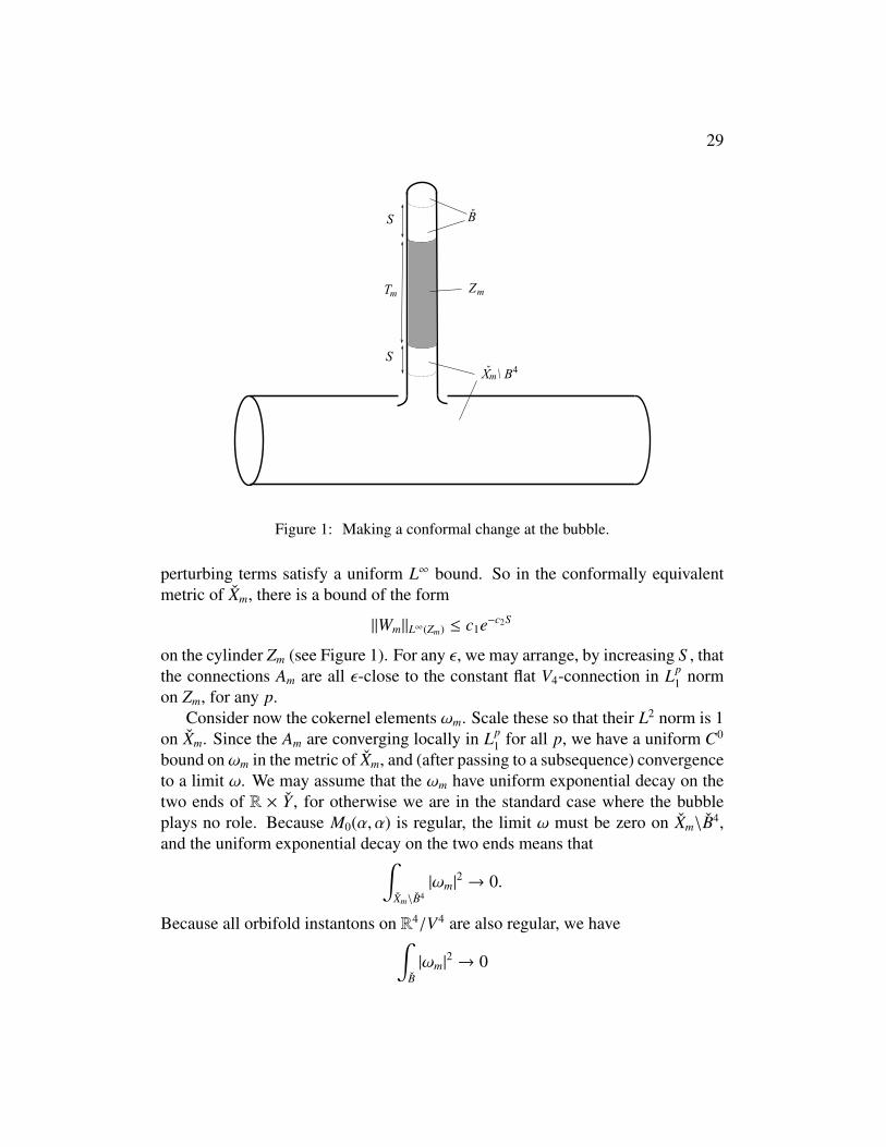
So let us suppose that Am converges to a point (p, A) in the Uhlenbeck com-pactification, where p is a point on a seam R×{v} and A ∈ M0(α, α) is the constantsolution. Let us apply a conformal change to R × Y , as indicated in Figure 1, sothat the new manifold Xm contains a cylinder on S 3/V4 of length Tm + 2S . Thelength S will be fixed and large. We can choose the lengths Tm and the centersof the conformal transformations so that the Am converge in the sense of brokentrajectories as Tm → ∞. In the limit, we obtain two pieces. We obtain an orbifoldinstanton on B = B4/V4 equipped with a cylindrical end (or equivalently S 4/V4),with action κ = 1/4; and we obtain the conformal transformation of the constantsolution A on (R × Y)\{p}.
On Xm, the equations satisfied by Am are of the form F+Am
= Wm, where Wm isobtained from the holonomy perturbation. In the original metric on R × Y , these
29
Figure 1: Making a conformal change at the bubble.
perturbing terms satisfy a uniform L∞ bound. So in the conformally equivalentmetric of Xm, there is a bound of the form
‖Wm‖L∞(Zm) ≤ c1e−c2S
on the cylinder Zm (see Figure 1). For any ε, we may arrange, by increasing S , thatthe connections Am are all ε-close to the constant flat V4-connection in Lp
1 normon Zm, for any p.
Consider now the cokernel elements ωm. Scale these so that their L2 norm is 1on Xm. Since the Am are converging locally in Lp
1 for all p, we have a uniform C0
bound onωm in the metric of Xm, and (after passing to a subsequence) convergenceto a limit ω. We may assume that the ωm have uniform exponential decay on thetwo ends of R × Y , for otherwise we are in the standard case where the bubbleplays no role. Because M0(α, α) is regular, the limit ω must be zero on Xm\B4,and the uniform exponential decay on the two ends means that∫
Xm\B4|ωm|
2 → 0.
Because all orbifold instantons on R4/V4 are also regular, we have∫B|ωm|
2 → 0

30
also. It follows that ∫Zm
|ωm|2 → 1.
However, ωm is converging to zero on the two boundary components of the cylin-der Zm = [0,Tm] × S 3/V4, and satisfies an equation which is schematically of theshape
d∗ωm + Am · ωm = Qm,
where Qm is the contribution coming from the non-local perturbation (and is there-fore dependent on the value ofω, on parts of Xm that are not in Zm). The Lp
1 conver-gence of the terms Am mean that the corresponding multiplication operators thatappear on the left can be taken to be uniformly small in operator norm, as opera-tors either from L2
1 to L2, or as operators on weighted Sobolev spaces, L21,δ → L2
δ,weighted by eδT . The terms Qm are also uniformly bounded in weighted L2 norms.So standard arguments (see [8] for example) establish that the L2 norm of ωm onlength-1 cylinders [t, t +1]× (S 3/V4) is uniformly controlled by a function that de-cays exponentially towards the middle of the cylinder. It follows that the integralof |ωm|
2 on Zm is also going to zero, which is a contradiction. �
The Proposition shows that we can construct 2-good perturbations for whichd2 = 0. It follows that, in fact, (C, d) is a complex for all 2-good perturbations,and therefore for all good perturbations. This is because, up to isomorphism, thecomplex C and boundary map d are stable under small changes in the perturbation,by the compactness of Cπ and M′
1(α, β). So we can always approximate a givengood perturbation by one for which the proof that d2 = 0 applies, without actuallychanging d. Thus, we have:
Proposition 3.2. The map d : C → C satisfies d2 = 0, for all good perturbationsπ.
We can now define the instanton Floer homology:
Definition 3.3. For any closed, oriented bifold Y with strong marking data µ, wedefine J(Y; µ) to be the homology of the complex (C, d) constructed above, for anychoice of orbifold Riemannian metric g and any good perturbation π. When Y isobtained from a 3-manifold Y with an embedded web K, we may write J(Y,K; µ).
31
3.4 Functoriality of J
In the above definition, the group J(Y; µ) depends on a choice of metric and per-turbation. As usual with Floer theories, the fact that J(Y; µ) is a topological invari-ant is a formal consequence of the more general functorial property of instantonhomology.
Let Y1 and Y0 be two 3-dimensional bifolds with orbifold metrics g1 and g0.Let X be an oriented cobordism from Y1 to Y0. Equip X with an orbifold metricthat is a product in a collar of each end. Let µ1 and µ0 be marking data for the twoends, and let ν be marking data for X that restricts to µ1 and µ0 at the boundary.Let π1 and π0 be good perturbations on Y1 and Y0. If we attach cylindrical ends toX and choose auxiliary perturbations in the neighborhoods of the two boundarycomponents [15, 14, 8], then we have moduli spaces of solutions to the perturbedanti-self-duality equations on the bifold:
M(X, ν;α, β). (9)
Here α and β are critical points for the perturbed Chern-Simons functional,i.e. generators for the chain complexes (C1, d1) and (C0, d0) associated with(Y1, µ1) and (Y0, µ0). Thus we can use (X; ν) to define a linear map
(C1, d1)→ (C0, d0)
between the respective complexes, by counting solutions to the perturbed equa-tions in zero-dimensional moduli spaces. The usual proof that the linear mapdefined in this way is a chain map involves moduli spaces only of dimension 0and 1. In particular, the codimension-2 bubbling phenomenon of Proposition 2.8does not enter into the argument (unlike the proof that d2 = 0). However, if thefoam Σ has tetrahedral points, then the codimension-1 bubbling phenomenon ofProposition 2.9 comes into play. That proposition tells us that the number of endsof each 1-dimensional moduli space that are accounted for by bubbling in the Uh-lenbeck compactification is a multiple of 4, and in particular even. So the usualproof carries over as long as we are using coefficients F.
In this way, (X; ν) defines a map on homology,
J(X; ν) : J(Y1; µ1)→ J(Y0; µ0).
Furthermore, a chain-homotopy argument shows that the map is independent ofthe choice of metric on the interior of X and is independent also of the auxiliaryperturbations on the cobordism.
32
Consider now the composition of two cobordisms. Suppose we have twocobordisms (X′; ν′) and (X′′; ν′′), where the first is a cobordism to (Y; µ) and thesecond is a cobordism from (Y; µ). This means that the restrictions of Eν′ andEν′′ to the common subset Eµ ⊂ Y are the same bundle (not just isomorphic), sotogether they define a bundle Eν′ ∪ Eν′′ . We can therefore join the cobordismscanonically to make a composite cobordism with marking data,
(X; ν) = (X′ ∪ X′′; ν′ ∪ ν′′).
In the above situation it is not always the case that
J(X; ν) = J(X′′; ν′′) ◦ J(X′; ν′). (10)
To see the reason for this, consider the problem of joining together marked con-nections. Suppose we have marked connection (E′, A′, σ′) and (E′′, A′′, σ′′) on(X′; ν′) and (X′′; ν′′) respectively. By restriction, we obtain two µ-marked connec-tions on (Y; µ), say (F′, B′, τ′) and (F′′, B′′, τ′′). Let us suppose these are isomor-phic: they define the same point in B(Y; µ). To avoid the issue of differentiability,let us also suppose that (E′, A′, σ′) coincides with the pull-back of (F′, B′, τ′) ina collar of Y , and similarly with E′′. Because the marking is strong, there is aunique isomorphism, which is a bundle isomorphism
φ : F′ → F′′
such that φ∗(B′′) = B′ and such that the map
ψ = (τ′′)−1φτ′ : Eµ → Eµ
lifts to determinant 1.These conditions on φ are not enough to allow us to construct a ν-marked
connection (E, A, σ) on the union X. Certainly we can use φ to glue E′ to E′′
along the common boundary, and the union of the connections A′ and A′′ willgive us a connection A. So we do have an unmarked SO(3) connection (E, A)on X. However, (E, A) does not have a ν-marking. Instead of having a bundleisomorphism
σ : Eν → E|Uν\Σ
we have a pair of bundle isomorphisms σ′ and σ′′ (essentially the maps σ′ andσ′′) defined over Uν′ and Uν′′ . To form σ, we would want σ′ and σ′′ to be equalon their common domain Eµ. Instead, we are only given that (σ′′)−1σ′|Eµ lifts todeterminant 1.
33
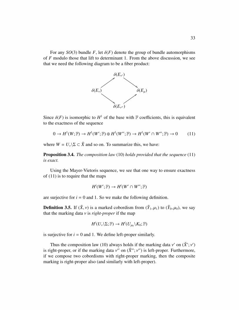
For any SO(3) bundle F, let δ(F) denote the group of bundle automorphismsof F modulo those that lift to determinant 1. From the above discussion, we seethat we need the following diagram to be a fiber product:
δ(Eν′)
$$δ(Eν)
::
$$
δ(Eµ)
δ(Eν′′)
::
Since δ(F) is isomorphic to H1 of the base with F coefficients, this is equivalentto the exactness of the sequence
0→ H1(W;F)→ H1(W ′;F) ⊕ H1(W ′′;F)→ H1(W ′ ∩W ′′;F)→ 0 (11)
where W = Uν\Σ ⊂ X and so on. To summarize this, we have:
Proposition 3.4. The composition law (10) holds provided that the sequence (11)is exact.
Using the Mayer-Vietoris sequence, we see that one way to ensure exactnessof (11) is to require that the maps
Hi(W ′;F)→ Hi(W ′ ∩W ′′;F)
are surjective for i = 0 and 1. So we make the following definition.
Definition 3.5. If (X, ν) is a marked cobordism from (Y1, µ1) to (Y0, µ0), we saythat the marking data ν is right-proper if the map
Hi(Uν\Σ;F)→ Hi(Uµ0\K0;F)
is surjective for i = 0 and 1. We define left-proper similarly.
Thus the composition law (10) always holds if the marking data ν′ on (X′; ν′)is right-proper, or if the marking data ν′′ on (X′′; ν′′) is left-proper. Furthermore,if we compose two cobordisms with right-proper marking, then the compositemarking is right-proper also (and similarly with left-proper).
34
Passing to the language of smooth 3-manifolds Y with embedded webs K, andsmooth 4-manifolds X with embedded foams Σ, we have the following descrip-tion. According to the definition, a foam comes with marked points (dots) on thefaces, but we consider first the case that there are no dots. There is a category inwhich an object is a quadruple (Y,K, µ, a), where Y is a closed, oriented, connected3-manifold, K is an embedded web, µ is strong marking data, and a is auxiliarydata consisting of a choice of orbifold metric g on a corresponding orbifold Yand a choice of good perturbation π ∈ P. A morphism in this category from(Y1,K1, µ1, a1) to (Y0,K0, µ0, a0) is an isomorphism class of compact, oriented, 4-manifold-with-boundary, X, containing a foam Σ and right-proper marking data ν,together with orientation-preserving identifications ι of (∂X, ∂Σ, ∂ν) with
(−Y1,K1, µ1) ∪ (Y0,K0, µ0).
The construction J defines a functor from this category to vector spaces over F.If only the auxiliary data ai differ, then there is a canonical product morphism
from (Y,K, µ, a1) to (Y,K, µ, a0), which is an isomorphism. So we can drop theauxiliary data a and take an object in our category to be a triple (Y,K, µ) and anmorphism to be (still) an isomorphism class of triples (X,Σ, ν).
Proposition 3.6. Let Co be the category in which an object is a triple (Y,K, µ),consisting a closed, connected, oriented 3-manifold Y, an embedded web K, andstrong marking data µ, and in which the morphisms are isomorphism classes offoam cobordisms (X,Σ, ν) with right-proper marking data ν. (Here again X is anoriented 4-manifold with boundary and Σ is an embedded foam, without dots.)Then J defines a functor from Co to vector spaces over F.
We use the terminology Co rather than C because we reserve C for the categoryin which the foams are allowed to have dots. We turn to this matter next.
3.5 Foams with dots
Until now, the foam Σ has been dotless. We now explain how to extend the defini-tion of the linear maps defined by cobordisms to the case of foams with dots. Fornow, we work in the general setting of cobordisms between 3-dimensional bifoldsequipped with strong marking data.
So consider a 4-manifold X with a foam Σ ⊂ X and strong marking data ν.Let X be a corresponding 4-dimensional Riemannian bifold. Let δ ∈ Σ be a point
35
lying on a face (a “dot”). Associated with δ is a real line bundle over the space ofconnections,
Lδ → Bl(X; ν),
defined as follows. Let Bδ ⊂ X be a ball neighborhood of δ, and consider markingdata µ given by the trivial bundle over Uµ = Bδ \ Σ. There is a double covering,
Bl(X; ν, µ)→ Bl(X; ν)
where the left-hand side is the space of isomorphism classes of bifold connections(E, A) equipped with two markings: a ν-marking τ, and a µ-marking σ. Thecovering map is the map that forgets σ:
(E, A, τ, σ) 7→ (E, A, τ).
The fact that this is a double cover is essentially the same point as in Lemma 2.4.We take Lδ to be the real line bundle associated to this double cover.
The line bundle Lδ can be regarded as being pulled back from the space ofconnections over a suitable open subset of X. Specifically, suppose Xδ ⊂ X is aconnected open set such that the two restriction maps
H1(Uν;F)→ H1(Xδ ∩ Uν;F)
andH1(Uµ;F)→ H1(Xδ ∩ Uµ;F)
are injective. On Xδ we have marking data νδ and µδ by restriction; and the linebundle Lδ can be regarded as pulled back via the restriction map
Bl(X; ν)→ Bl(Xδ; νδ).
We will choose Xδ so that it is disjoint from the foam and the boundary of X.(Think of a regular neighborhood of a collection of loops in X.)
In this way, given a collection of points δi (i = 1, . . . , n), we obtain a collectionof real line bundles Lδi which we may regard as pulled back from spaces of markedconnections over disjoint open sets Xδi ⊂ X. Let si be a section of Lδi that is alsopulled back from Xδi , and let
V(δi) ⊂ Bl(X; ν)
36
be its zero-set. If X is a bifold cobordism to which we attach cylindrical ends, wecan then consider the moduli spaces of solutions to the perturbed anti-self-dualityequations (9) cut down by the V(δi):
M(X, ν;α, β) ∩ V(δ1) ∩ · · · ∩ V(δn).
The sections sδi can be chosen so that all such intersections are transverse. Thedisjointness of the Xδi ensures the necessary compactness properties when bubblesoccur and these moduli spaces define chain maps in the usual way. The resultingmaps on homology are the required maps defined by the cobordism with dotsδ1, . . . , δn on the foam. We have:
Proposition 3.7. The above construction extends J from the category Co of dotlessfoams to the category C of foams with dots, in which an object is a triple (Y,K, µ),consisting a closed, connected, oriented 3-manifold Y, an embedded web K, andstrong marking data µ, and in which the morphisms are isomorphism classes offoam cobordisms (X,Σ, ν) with right-proper marking data ν.
As a special case of the construction, given a web K ⊂ Y we can define acollection of operators on J(Y,K, µ), one for each edge of K:
Definition 3.8. For each edge e of a web K, we write
ue : J(Y,K, µ)→ J(Y,K, µ)
for the operator corresponding to cylindrical cobordism with a single dot on theface corresponding to the edge e.
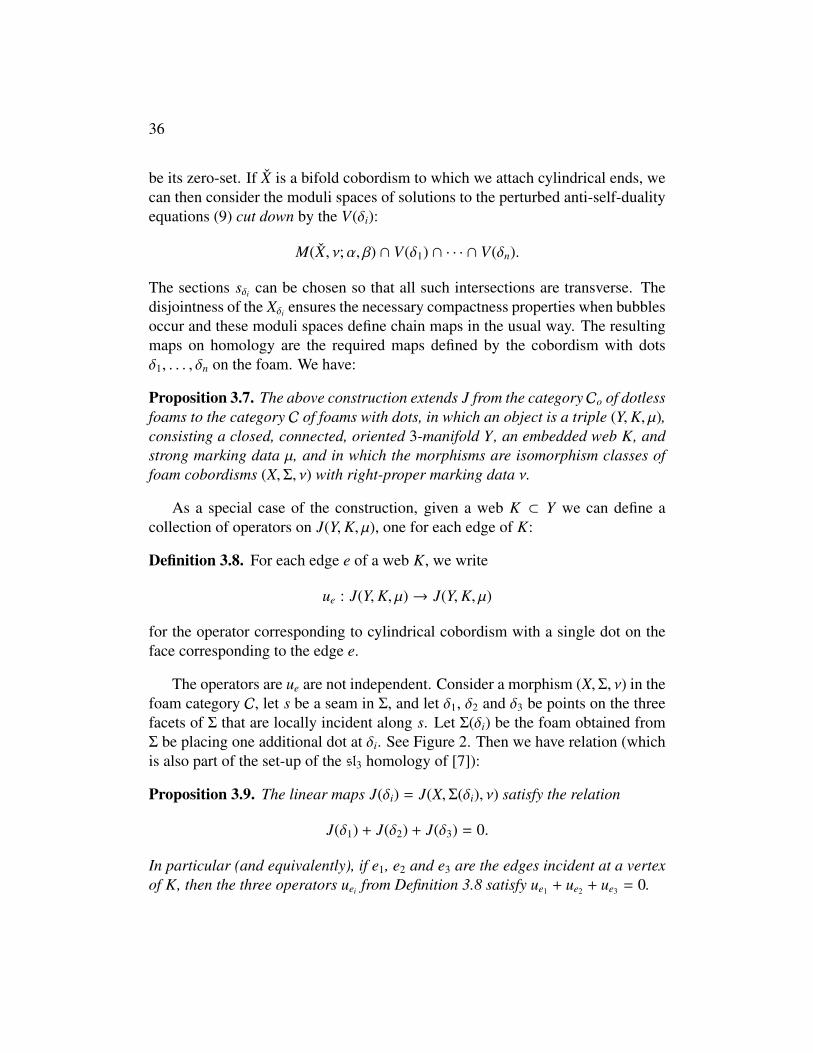
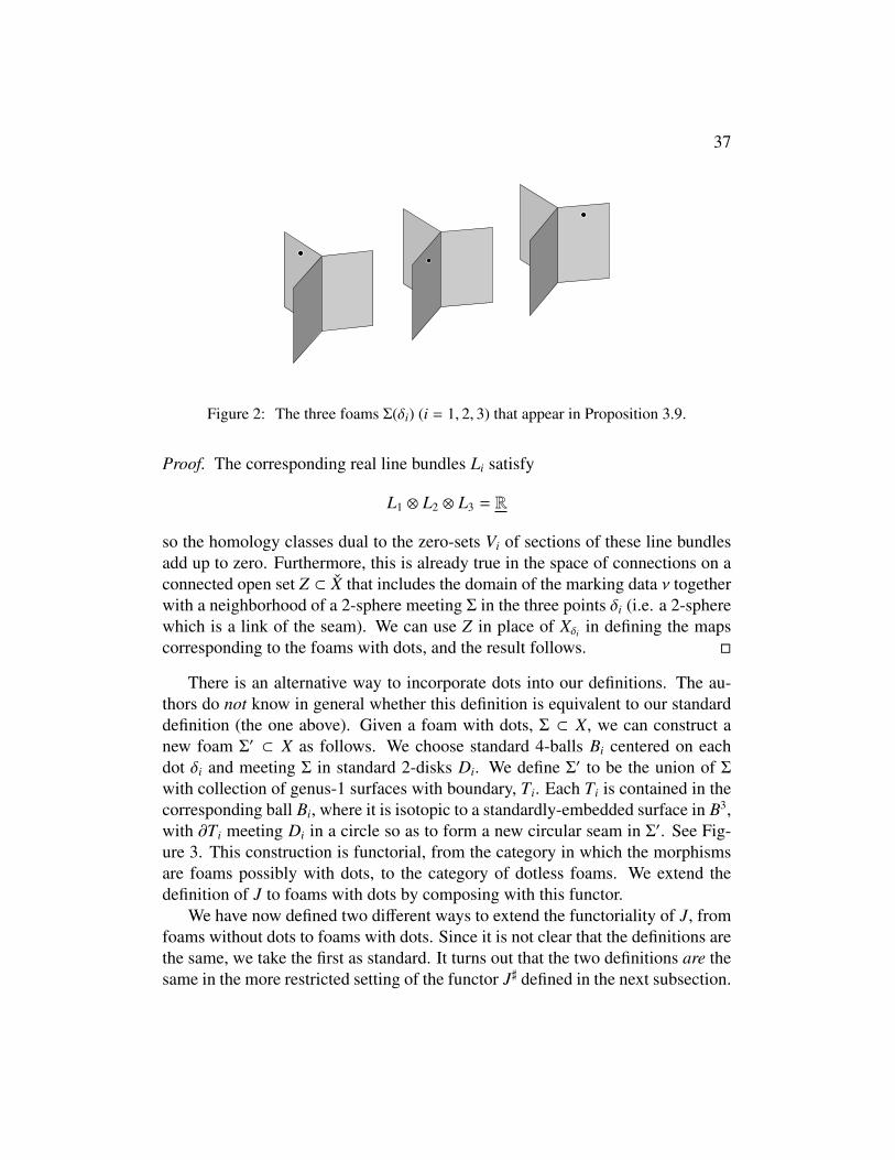
The operators are ue are not independent. Consider a morphism (X,Σ, ν) in thefoam category C, let s be a seam in Σ, and let δ1, δ2 and δ3 be points on the threefacets of Σ that are locally incident along s. Let Σ(δi) be the foam obtained fromΣ be placing one additional dot at δi. See Figure 2. Then we have relation (whichis also part of the set-up of the sl3 homology of [7]):
Proposition 3.9. The linear maps J(δi) = J(X,Σ(δi), ν) satisfy the relation
J(δ1) + J(δ2) + J(δ3) = 0.
In particular (and equivalently), if e1, e2 and e3 are the edges incident at a vertexof K, then the three operators uei from Definition 3.8 satisfy ue1 + ue2 + ue3 = 0.
37
Figure 2: The three foams Σ(δi) (i = 1, 2, 3) that appear in Proposition 3.9.
Proof. The corresponding real line bundles Li satisfy
L1 ⊗ L2 ⊗ L3 = R
so the homology classes dual to the zero-sets Vi of sections of these line bundlesadd up to zero. Furthermore, this is already true in the space of connections on aconnected open set Z ⊂ X that includes the domain of the marking data ν togetherwith a neighborhood of a 2-sphere meeting Σ in the three points δi (i.e. a 2-spherewhich is a link of the seam). We can use Z in place of Xδi in defining the mapscorresponding to the foams with dots, and the result follows. �
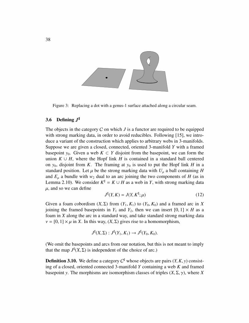
There is an alternative way to incorporate dots into our definitions. The au-thors do not know in general whether this definition is equivalent to our standarddefinition (the one above). Given a foam with dots, Σ ⊂ X, we can construct anew foam Σ′ ⊂ X as follows. We choose standard 4-balls Bi centered on eachdot δi and meeting Σ in standard 2-disks Di. We define Σ′ to be the union of Σ
with collection of genus-1 surfaces with boundary, Ti. Each Ti is contained in thecorresponding ball Bi, where it is isotopic to a standardly-embedded surface in B3,with ∂Ti meeting Di in a circle so as to form a new circular seam in Σ′. See Fig-ure 3. This construction is functorial, from the category in which the morphismsare foams possibly with dots, to the category of dotless foams. We extend thedefinition of J to foams with dots by composing with this functor.
We have now defined two different ways to extend the functoriality of J, fromfoams without dots to foams with dots. Since it is not clear that the definitions arethe same, we take the first as standard. It turns out that the two definitions are thesame in the more restricted setting of the functor J] defined in the next subsection.
38
Figure 3: Replacing a dot with a genus-1 surface attached along a circular seam.
3.6 Defining J]
The objects in the category C on which J is a functor are required to be equippedwith strong marking data, in order to avoid reducibles. Following [15], we intro-duce a variant of the construction which applies to arbitrary webs in 3-manifolds.Suppose we are given a closed, connected, oriented 3-manifold Y with a framedbasepoint y0. Given a web K ⊂ Y disjoint from the basepoint, we can form theunion K ∪ H, where the Hopf link H is contained in a standard ball centeredon y0, disjoint from K. The framing at y0 is used to put the Hopf link H in astandard position. Let µ be the strong marking data with Uµ a ball containing Hand Eµ a bundle with w2 dual to an arc joining the two components of H (as inLemma 2.10). We consider K] = K ∪ H as a web in Y , with strong marking dataµ, and so we can define
J](Y,K) = J(Y,K]; µ) (12)
Given a foam cobordism (X,Σ) from (Y1,K1) to (Y0,K0) and a framed arc in Xjoining the framed basepoints in Y1 and Y2, then we can insert [0, 1] × H as afoam in X along the arc in a standard way, and take standard strong marking dataν = [0, 1] × µ in X. In this way, (X,Σ) gives rise to a homomorphism,
J](X,Σ) : J](Y1,K1)→ J](Y0,K0).
(We omit the basepoints and arcs from our notation, but this is not meant to implythat the map J](X,Σ) is independent of the choice of arc.)
Definition 3.10. We define a category C] whose objects are pairs (Y,K, y) consist-ing of a closed, oriented connected 3-manifold Y containing a web K and framedbasepoint y. The morphisms are isomorphism classes of triples (X,Σ, γ), where X
39
is a connected oriented 4-manifold, Σ is a foam, and γ is a framed arc joining thebasepoints. Thus J] is a functor,
J] : C] → (Vector spaces over F).
by composing “Sharp” with J.
Sometimes we will regard J] as defining a functor from the category of websin R3 and isotopy classes of foams in [0, 1]×R3, by compactifying R3 and puttingthe framed basepoint at infinity. We will then just write J](K) etc. for a web K inR3.
There is a variant of this definition that we can consider. We can define
I] : C] → (Vector spaces over F)
in much the same way, except that instead of using the marking µ with Uµ = B3
as above, we instead use the marking µ′ with Uµ′ the whole of the three-manifoldY . We still take Eµ′ to be a bundle with w2 dual to the same arc. Thus,
I](Y,K) = J(Y,K ∪ H; µ′). (13)
In the case that K has no vertices, this is precisely the knot invariant I](K) definedin [15], except that we are now using F coefficients. Over F at least, our definitionextends that of [15] by allowing embedded webs rather than just knots and links.
There is another simple abbreviation to our notation that will be convenient.It is a straightforward fact that J](S 3, ∅) is F (see below), so a cobordism from(S 3, ∅) to (Y,K) in the category C] determines a vector in J](Y,K). This allows usto adopt the following two conventions:
Definition 3.11. Let X be compact, oriented 4-manifold with boundary the con-nected 3-manifold Y , and let Σ be a foam in X with boundary a web K ⊂ Y . Let abasepoint y ∈ Y be given. Then we write J](X,Σ) for the element of J](Y,K) cor-responding the cobordism from (S 3, ∅) to (Y,K) obtained from (X,Σ) by removinga ball from X and connecting a point on its boundary to y by an arc.
Similarly, given closed, connected manifold X containing a closed foam Σ, wewill write J](X,Σ) for the scalar in F corresponding to the morphism from (S 3, ∅)to itself, obtained from (X,Σ) by removing two balls disjoint from Σ and joiningthem by an arc. We refer to J](X,Σ) in this context as the J]-evaluation of theclosed foam.
40
We can also use the language of bifolds directly, rather than manifolds withembedded webs. We will consider 3-dimensional bifolds Y with a framed base-point y0 (in the smooth part of Y , not an orbifold point). For such a Y , we writethe corresponding invariant as J](Y). Given a bifold cobordism X from Y1 to Y0
and a framed arc joining basepoints in these, we obtain a homomorphism
J](X) : J](Y1)→ J](Y0).
We will also allow the conventions of Definition 3.11 in this context, and so talkabout J](X) for an orbifold with connected boundary, or with no boundary.
3.7 Simplest calculations
We have the following three simple examples of calculation of J] for webs K inR3.
Proposition 3.12. We have the following special cases.
(a) If K is the empty web in R3, then J](K) = F.
(b) If the web K ⊂ R3 has an embedded bridge, then J](K) = 0.
Proof. In both cases, we start by applying Lemma 2.10, which tells us that theunperturbed set of critical points for the Chern-Simons functional for (S 3,K∪H, µ)can be identified with
R](K) = { ρ : π1(R3\K)→ SO(3) | ρ(me) has order 2 for all edges e }.
In the first case of the proposition, the representation variety is a single point (thetrivial representation of the trivial group), and this point is non-degenerate as acritical point of Chern-Simons. So J] has rank 1.
In the case of an embedded bridge e, the meridian me is null-homotopic, sothere is no ρ such that ρ(me) has order 2. The representation variety is thereforeempty, and J](K) = 0. �
4 Excision
4.1 Floer’s excision argument
Floer’s excision theorem [2, 13] can be applied in the setting of the SO(3) in-stanton homology J. We spell out statements of the basic result for cutting and
41
gluing along tori (which is the original version), as well as cutting an gluing along2-spheres with three orbifold points.
Let (Y , µ) be a 3-dimensional bifold containing a web with strong markingdata µ. We will temporarily allow the case that Y is not connected, in which casethe marking data µ is strong only if its restriction to each component of Y is strong.Let T1, T2 be disjoint, oriented, embedded 2-tori in Uµ. (In particular, they lie inthe smooth part of Y .) We require the additional property that the restrictions, Ei,of the marking bundle Eµ to the tori Ti have non-zero w2. Pick an identificationbetween the tori, T1 → T2, and lift it to an isomorphism between the bundles.By cutting along T1, T2 and regluing (using the preferred identifications in anorientation-preserving way), we obtain a new object (Y ′, µ′). In Y ′, we also endup with a pair of embedded tori T ′1 and T ′2.
We will be concerned with the case that T1 and T2 lie in distinct componentsY1, Y2 of Y . In this case, cutting along Ti cuts Yi into pieces Y+
i and Y−i . The newbifold Y ′ has components Y ′1 = Y+
1 ∪ Y−2 etc.
Theorem 4.1 (Floer’s excision). In the above setting, when T1, T2 are separatingtori in distinct components Y1, Y2, we have
J(Y , µ) = J(Y ′, µ′).
Proof. The proof is a straightforward adaption of the original argument of Floer[2]. The case of separating tori was given in [15]. �
There is a variant of the excision argument, in which the tori T1, T2 are re-placed by spheres S 1, S 2 each with three orbifold points. That is, we ask that S 1,S 2 are 2-dimensional sub-orbifolds of Y , meeting the web K of orbifold pointsin three points each. We still require that S i \ K lies in Uµ, and require the sameseparation hypotheses. By cutting and gluing, we form (Y ′, µ′) just as in the toruscase. The same result holds:
Theorem 4.2. In the above setting, when S 1, S 2 are separating 3-pointed spheresin distinct components Y1, Y2, we have
J(Y , µ) = J(Y ′, µ′).
Proof. This adaptation of the excision theorem is contained in [21], in a versionfor any number orbifold points on the spheres. In the case of 3 points, the argu-ment from the torus case needs no serious adaptation: the essential point is theexistence of a unique SO(3) connection on the 2-dimensional orbifold. �
42
Remark. In the non-separating case, some extra care is needed to obtain correctstatements, because of the double-covers that correspond to possibly differentstrong marking data.
4.2 Applications of excision
If Y1 and Y2 are bifolds with framed basepoints (at non-orbifold points), then thereis a preferred connected sum Y = Y1#Y2 obtained by summing at the basepoints.We can give the new bifold a preferred framed basepoint, on the 2-sphere wherethe sum is made. Given bifold cobordisms with framed arcs joining the base-points, say
Xi : Yi → Y ′i , (i = 1, 2),
then we can form a cobordism
X : Y → Y
by summing along the embedded arcs.
Proposition 4.3. In the above situation, we have an isomorphism
J](Y) = J](Y1) ⊗ J](Y2).
Furthermore, this isomorphism is natural for the maps corresponding to cobor-disms Xi as above, so that
J](X) = J](X1) ⊗ J](X2).
The same applies with I] in place of J].
Corollary 4.4. Suppose K = K1∪K2 is a split web in R3, meaning that there is anembedded 2-sphere S which separates K1 from K2. Then there is an isomorphism,
J](K) = J](K1) ⊗ J](K2).
Moreover, if Σ is a split cobordism, meaning that Σ = Σ1 ∪ Σ2 and Σ is disjointfrom [0, 1] × S , then
J](Σ) = J](Σ1) ⊗ J](Σ2).
The same applies with I] in place of J].
43
These excision results will be often applied through the following corollaries,which we state first in the language of bifolds. Let Q be a closed, oriented, con-nected 3-dimensional bifold. Let Pi be 4-dimensional bifolds with boundary Q,for i = 1, . . . , n. In the notation of Definition 3.11, these have invariants
J](Pi) ∈ J](Q).
Suppose that we also have a collection of cobordisms
Xi : Y → Y ′, i = 1, . . . , n,
such that Xi contains in its interior an embedded copy of Pi. Suppose the comple-ments Xi \ int(Pi) are all identified, in a way that restricts to the identity on theircommon boundary components Y , Y ′ and Q. We then have
Corollary 4.5. If the elements of J](Q) defined by the bifolds Pi satisfy a relation
n∑i=1
J](Pi) = 0,
then it follows also thatn∑
i=1
J](Xi) = 0
as maps from J](Y) to J](Y ′). The same applies with I] in place of J].
We next restate the last corollary as it applies to the case of webs. Let W be aweb in a connected 3-manifold Q. For i = 1, . . . , n, let Pi be a connected, oriented4-manifold with boundary Q, and let Vi ⊂ Pi be a foam with boundary W. Thesedetermine elements
J](Pi,Vi) ∈ J](Q,W).
Suppose we also have a collection of foam cobordisms
(Xi,Σi) : (Y,K)→ (Y ′,K′).
Suppose that each (Xi,Σi) contains an interior copy of (Pi,Vi), and that the com-plements are all identical. We then have the following restatement:
Corollary 4.6. If∑
J](Pi,Vi) = 0, then∑
J](Xi,Σi) = 0, as maps from J](Y,K)→J](Y ′,K′). The same holds with I] in place of J].

44
5 Calculations
5.1 The unknot and the sphere with dots
Proposition 5.1. For the unknotted circle, the homology J](K) has rank 3.Equipped with the operator ue : J](K) → J](K) (see Definition 3.8), it is iso-morphic to F[u]/u3 as a module over the polynomial algebra.
Proof. The representation variety R](K) is a copy of RP2 (as in section 2.9). Wecan choose a small, good perturbation π so that fπ restricts to a standard Morsefunction on RP2, leading to three critical points α0, α1 and α2. For the specialcase of the unknot the Floer homology is Z/4 graded, and the only 1-dimensionalmoduli spaces are therefore M1(α2, α1) and M1(α1, α0). These moduli spaces ap-proximate the Morse trajectories on RP2, so J](K) = H∗(RP2;F), which has rank3.
For the module structure, a dot δ on the knot, the double-cover which corre-sponds to the line bundle Lδ is the non-trivial double cover of RP2. The calculationonly involves Morse trajectories on RP2, so the result is the same as for a calcula-tion of the cap product with the one-dimensional cohomology class acting on thehomology of RP2. �
As a simple application of Corollary 4.6, we have the following result.
Proposition 5.2. Let K ⊂ Y be a web, let e be an edge of K, and ue the corre-sponding operator on J](Y,K). (See Definition 3.8.) Then u3
e = 0.
Proof. We apply Corollary 4.6, to the case that M = B3, the web W is a single arcin B3, and (N,V) is a disk with 3 dots. We see that it is sufficient to check that adisk with three dots defines the zero element in J](K) when K is the unknot. Thisin turn follows from Proposition 5.1. �
The calculation of J] with its module structure for the unknot K is closelyrelated to the evaluation of the closed foam S (k), consisting of an unknotted 2-sphere S in R4 or S 4, with k dots. Before continuing, it will be useful to makesome general remarks about closed foams.
A closed foam Σ in S 4 evaluates to 0 or 1,
J](Σ) ∈ F
by the convention of Definition 3.11. Because the definition involves counting so-lutions in 0-dimensional moduli spaces, we can read off the action κ of the relevant
45
solutions from the dimension formula (5). Taking account of the codimension-1constraints corresponding to the dots on Σ, and writing k for the number of dots,we must have
8κ + χ(Σ) +12
Σ · Σ −12|τ| − k = 0.
This gives us some necessary conditions for a non-zero evaluation. Since κ isnon-negative, we must have
k ≥ χ(Σ) +12
Σ · Σ −12|τ|. (14)
We evaluate J](Σ) for a sphere with dots.
Proposition 5.3. Let S (k) denote the unknotted 2-sphere with k dots, as a foam inR4 or S 4. Then J](S (k)) = 1 if k = 2 and is 0 otherwise.
Proof. The fact that J](S (k)) = 0 for k ≥ 3 follows from Proposition 5.2. Theinequality (14) requires k ≥ 2 in this case. So S (2) is the only case where theevaluation can be non-zero. Furthermore, for the case k = 2, the action κ for therelevant moduli spaces is zero: we are looking for flat connections. As in the caseof the unknot considered earlier, the representation variety of flat connections isRP2, and the real line bundle over RP2 corresponding to each dot is the non-trivialone. So J](S (2)) is obtained by evaluating the square of the basic 1-dimensionalclass on RP2, and the answer is 1 as claimed. �
If D(k) is a 2-disk in B4 with boundary a standard circle in S 3, regarded as afoam with k dots, then a formal corollary of the above proposition is:
Corollary 5.4. The elements J](D(0)), J](D(1) and J](D(2)) are a basis for J](K),where K ⊂ S 3 is a standard circle (the unknot).
Using Corollary 4.4, we obtain from this a simple criterion for testing whetheran element of the Floer homology of an unlink is zero:
Lemma 5.5. Let (S 3,Kn) be an n-component unlink in the 3-sphere. Let (X,Σi) bewebs with boundary (S 3,Kn). Then, in order that a relation∑
i
J](X,Σi) = 0
holds in J](S 3,Kn), it is necessary and sufficient to test, for all n-tuples (k1, . . . , kn) ∈{0, 1, 2}n, that the relation ∑
i
J](X, Σi) = 0,
46
holds in F, where X is obtained from X by adding a ball, and Σi is obtained fromΣi by adding a standard disk with km dots, D(km) ⊂ B4, to the m’th component ofKn.
5.2 The theta foam and the theta web
A theta foam is a closed foam formed from three disks in R3 meeting along a com-mon circle, the seam. We write Θ for a typical theta-foam in R4, and Θ(k1, k2, k3)for the same foam with the addition of ki dots on the i’th disk.
Proposition 5.6. For the theta foam with dots, Θ(k1, k2, k3), we have
Θ(k1, k2, k3) = 1
if (k1, k2, k3) = (0, 1, 2) or some permutation thereof. In all other cases the evalu-ation is zero.
Proof. In the case of the theta foam in R4, any solution of the equation has actionsatisfying 4κ ∈ Z. One can verify this by considering a bifold connection on(S 4,Θ): any such gives rise to an ordinary SO(3) action of the V4-cover S 4, wherethe action must be an integer. The relation in Proposition 3.9 tells us that
J](Θ(k1, k2, k3)) = J](Θ(k1 − 1, k2 + 1, k3)) + J](Θ(k1 − 1, k2, k3 + 1))
as long as k1 , 0. So the evaluation for Θ(k1, k2, k3) will be completely deter-mined once we know the evaluations for the cases with k1 = 0. So we examineΘ(0, k2, k3). For a non-zero evaluation, we require ki ≤ 2, because of Proposi-tion 5.2. The inequality (14) requires k2 + k3 ≥ 3 in this case. Furthermore, k2 + k3
must be odd, because 4κ is an integer. These constraints mean we need only lookat Θ(0, 1, 2), and here the moduli space we are concerned with is a moduli spaceof flat connections. The representation variety in this example is the flag manifoldF = SO(3)/V4, and the three real line bundles corresponding to dots on the threesheets are the three tautological line bundles L1, L2, L3 on F. The evaluation ofΘ(0, 1, 2) is therefore equal to⟨
w1(L2)w1(L3)2, [F]⟩,
which is 1. �
Let K be a theta web. Corresponding to the three edges, there are three opera-tors ui : J](K)→ J](K).
47
Proposition 5.7. For the theta web K, the instanton homology J](K) can be iden-tified with the ordinary F homology of the flag manifold F = SO(3)/V4 in sucha way that the operators ui correspond to the operation of cap product with theclasses w1(Li), where L1, L2, L3 are the tautological line bundle on the flag man-ifold. Concretely, this means that the dimension is 6 and that the instanton ho-mology is a cyclic module over the algebra generated by the ui which satisfy therelations
u1 + u2 + u3 = 0u1u2 + u2u3 + u3u1 = 0
u1u2u3 = 0.
Proof. The representation variety for the theta web is the flag manifold, so therank of the instanton homology is at most 6. On the other hand, we can seethat the rank is at least 6 as follows. Consider a theta-foam cut into two piecesby a hyperplane, so as to have cobordisms Θ− from ∅ to K and Θ+ from K to∅. Putting ki dots on the i’th facet of Θ± and applying J], we obtain vectorsx−(k1, k2, k3) in J](K) and covectors x+(k1, k2, k3). The pairings between these canbe evaluated using the knowledge of the closed theta foam (Proposition 5.6). Ifwe restrict to the elements x±(0, k1, k2) with k1 ≤ 1 and k2 ≤ 2, then the resultingmatrix of pairings is non-singular. So the corresponding 6 elements x−(0, k1, k2)in J](K) are independent. The relations satisfied by the operators ui can be readoff similarly. �
As a corollary of the above proposition and excision, we have:
Proposition 5.8. Let K be any web in a 3-manifold Y, and let u1, u2, u3 be theoperators corresponding to three edges of K that are incident at a common vertex.Then the operators satisfy the same relations,
u1 + u2 + u3 = 0u1u2 + u2u3 + u3u1 = 0
u1u2u3 = 0.(15)
In particular, any monomial ua1ub
2uc3 of total degree 4 or more is zero.
5.3 The tetrahedron web and its suspension
Let K be the tetrahedron web: the graph drawn in Figure 4, with the edges labeledas shown. Let T ⊂ B4 be the cone on K, regarded as a foam with one tetrahedral
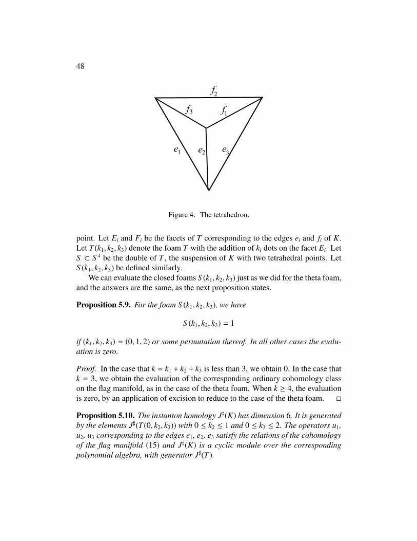
48
Figure 4: The tetrahedron.
point. Let Ei and Fi be the facets of T corresponding to the edges ei and fi of K.Let T (k1, k2, k3) denote the foam T with the addition of ki dots on the facet Ei. LetS ⊂ S 4 be the double of T , the suspension of K with two tetrahedral points. LetS (k1, k2, k3) be defined similarly.
We can evaluate the closed foams S (k1, k2, k3) just as we did for the theta foam,and the answers are the same, as the next proposition states.
Proposition 5.9. For the foam S (k1, k2, k3), we have
S (k1, k2, k3) = 1
if (k1, k2, k3) = (0, 1, 2) or some permutation thereof. In all other cases the evalu-ation is zero.
Proof. In the case that k = k1 + k2 + k3 is less than 3, we obtain 0. In the case thatk = 3, we obtain the evaluation of the corresponding ordinary cohomology classon the flag manifold, as in the case of the theta foam. When k ≥ 4, the evaluationis zero, by an application of excision to reduce to the case of the theta foam. �
Proposition 5.10. The instanton homology J](K) has dimension 6. It is generatedby the elements J](T (0, k2, k3)) with 0 ≤ k2 ≤ 1 and 0 ≤ k3 ≤ 2. The operators u1,u2, u3 corresponding to the edges e1, e2, e3 satisfy the relations of the cohomologyof the flag manifold (15) and J](K) is a cyclic module over the correspondingpolynomial algebra, with generator J](T ).
49
Proof. The representation variety of K] is again the flag manifold, so the dimen-sion of J](K is at most 6. On the other hand, we can compute the pairings of theclasses J](T (k1, k2, k3) with all their doubles, using our knowledge of S (k1, k2, k3),and from this we see that the six elements J](0, k2, k3) for k2 and k3 in the givenrange are independent. So the rank is exactly 6. �
To complete our description of J](K), we must describe the operators corre-sponding to the other three edges, f1, f2, f3.
Proposition 5.11. The operators v1, v2, v3 on J](K) corresponding to the edgesf1, f2, f3 are equal to u1, u2, u3 respectively.
Proof. We will show that v1 = u1. Let S 1 denote the foam S equipped with asingle dot on the facet corresponding to f1. Let S 1(k1, k2, k3) denote the samefoam with addition dots on the facets corresponding to the edges ei. It will sufficeto show that
S 1(0, k2, k3) = S (1, k2, k3)
for all values of k2 and k3. As usual if 1 + k2 + k3 ≤ 2, then the evaluation is zero,while if 1+k2 +k3 = 3 we are evaluating an ordinary cohomology class on the flagmanifold. Since the line bundle corresponding to a dot on f1 is the same as theline bundle corresponding to a dot on e1, equality does hold when 1 + k2 + k3 = 3.The only case still in doubt is when 1 + k2 + k3 = 4, and the only potentiallynon-zero evaluations here are S 1(0, 1, 2) or S 1(0, 2, 1) (which are certainly equal,by symmetry). We must show that S 1(0, 1, 2) = 0.
Suppose instead that S 1(0, 1, 2) = 1. With this complete information aboutS 1(0, k1, k2) we can evaluate the matrix elements of v1 on our standard basis, andwe find that v1 + u1 = 1 as operators on J](K). But u1 and v1 are both nilpotentbecause u3
1 = v31 = 0, so this is impossible. �
5.4 Upper bounds for some prisms
Let Ln be the planar trivalent graph formed from two concentric n-gons with edgesjoining each vertex of the outer n-gon to the corresponding vertex of the inner n-gon. We call Ln the n-sided prism. Later we will be able to determine J](Ln)entirely; but for now we can obtain upper bounds on the rank of Ln for small n.These upper bounds will be used later, in section 6, after which we will have thetools to show that these upper bounds are exact values.
Lemma 5.12. The dimension of J](Ln) is at most 12 for n = 2, at most 6 for n = 3,and at most 24 for n = 4.
50
Proof. For n = 2 and n = 3, the representation varieties R](Ln) consists of 2 (re-spectively, 1) copy of the flag manifold SO(3)/V4. These are the orbits of the flatconnections with image V4, of which there are two distinct classes in the case ofL2. In both cases, the Chern-Simons function is Morse-Bott, so an upper boundfor the ranks of J](Ln) are the dimension of the ordinary homology of the repre-sentation variety, which are 12 and 6 respectively.
For the case n = 4, the representation variety is not Morse-Bott. The un-basedrepresentation variety R(L4) consists of three arcs with one endpoint in common.The common point and the three other endpoints of the arc correspond to V4 rep-resentations in R(L4). The interiors of the three arcs parametrize flat connectionswith image contained in O(2) but not in V4. Using an explicit holonomy pertur-bation, one can perturb the Chern-Simons function by a small function f whichhas critical points at the common endpoint and the three other endpoints of thearc, but whose restriction to the interiors of the three arcs has no critical points.After adding this perturbation, the critical set in R](L4) is Morse-Bott and com-prises four copies of SO(3)/V4. We omit the details for this explicit construction,because there is a more robust argument based on the exact triangle satisfied byJ] which will be treated in a subsequent paper [9]. �
6 Relations
Sections 6.1–6.4 establish properties of J] that aid calculation. With the exceptionof the triangle relation (section 6.3), these properties (and some of their proofs)are motivated by [7], where similar properties of Khovanov’s sl3 homology areeither proved or (in the case of the neck-cutting relation) taken as axioms.
6.1 The neck-cutting relation
The following proposition describes what happens when a foam is surgered alongan embedded disk. The statement of the proposition is illustrated in Figure 5. Seealso [7].
Proposition 6.1 (Neck-cutting). Let (X,Σ) be a cobordism defining a morphismin C]. Suppose that X contains an embedded disk D whose boundary lies in theinterior of a facet of Σ, which it meets transversely. Suppose that the trivializa-tion of the normal bundle to D at the boundary which Σ determines extends to atrivialization over the disk. Let Σ′ be the foam obtained by surgering Σ along D,
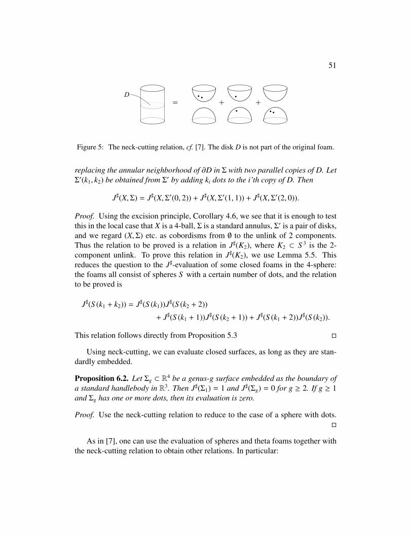
51
Figure 5: The neck-cutting relation, cf. [7]. The disk D is not part of the original foam.
replacing the annular neighborhood of ∂D in Σ with two parallel copies of D. LetΣ′(k1, k2) be obtained from Σ′ by adding ki dots to the i’th copy of D. Then
J](X,Σ) = J](X,Σ′(0, 2)) + J](X,Σ′(1, 1)) + J](X,Σ′(2, 0)).
Proof. Using the excision principle, Corollary 4.6, we see that it is enough to testthis in the local case that X is a 4-ball, Σ is a standard annulus, Σ′ is a pair of disks,and we regard (X,Σ) etc. as cobordisms from ∅ to the unlink of 2 components.Thus the relation to be proved is a relation in J](K2), where K2 ⊂ S 3 is the 2-component unlink. To prove this relation in J](K2), we use Lemma 5.5. Thisreduces the question to the J]-evaluation of some closed foams in the 4-sphere:the foams all consist of spheres S with a certain number of dots, and the relationto be proved is
J](S (k1 + k2)) = J](S (k1))J](S (k2 + 2))
+ J](S (k1 + 1))J](S (k2 + 1)) + J](S (k1 + 2))J](S (k2)).
This relation follows directly from Proposition 5.3 �
Using neck-cutting, we can evaluate closed surfaces, as long as they are stan-dardly embedded.
Proposition 6.2. Let Σg ⊂ R4 be a genus-g surface embedded as the boundary of
a standard handlebody in R3. Then J](Σ1) = 1 and J](Σg) = 0 for g ≥ 2. If g ≥ 1and Σg has one or more dots, then its evaluation is zero.
Proof. Use the neck-cutting relation to reduce to the case of a sphere with dots.�
As in [7], one can use the evaluation of spheres and theta foams together withthe neck-cutting relation to obtain other relations. In particular:
52
Proposition 6.3 (Bubble-bursting). Let D be an embedded disk in the interiorof a facet of a foam Σ ⊂ X. Let γ be the boundary of D, and let Σ′ be the foamΣ′ = Σ∪D′, where D′ is a second disk meeting Σ along the circle γ, so that D∪D′
bounds a 3-ball. Let Σ′(k) denote Σ′ with k dots on D′. Let Σ(k) denote Σ with kdots on D. Then we have
J](Σ′(k)) = J](Σ(k − 1))
for k = 1 or 2, and J](Σ′(k) = 0 otherwise.
Proof. Let γ1 be a circle parallel to γ in Σ \ D. Apply the neck-cutting relation tothe surgery of Σ′ along a disk with boundary γ′. The surgered foam is the unionof a foam isotopic to Σ with theta foam. �
Instead of adding a disk D′ to Σ, we can add a standard genus-1 surface T withboundary γ. The resulting foam Σ ∪ T was considered earlier in section 3.5. LetΣ(k) again denote Σ with k dots in the disk. Then we have
Proposition 6.4. In the above situation, J](Σ ∪ T ) = J](Σ(1)).
Proof. By two surgeries, the foam Σ∪ T becomes a split union of Σ, a theta foamand a standard torus. Apply the neck-cutting relation and the known evaluationsfor theta foams and tori. �
The proposition above justifies the alternative description of how to incorpo-rate dots on foams, from section 3.5.
6.2 The bigon relation
Let K ⊂ Y be a web containing a bigon: a pair of edges spanning standard disk inY , and let K′ be obtained from K by collapsing the bigon to a single edge. (SeeFigure 6.)
Proposition 6.5. The dimension of J](K) is twice the dimension of J](K′).
Proof. The proof mirrors Khovanov’s argument in [7]. There four standard mor-phisms,
A, B : K′ → KC,D : K → K′
as shown in Figure 6, and these give rise to maps

53
Figure 6: Four morphisms for the bigon relation.
a, b : J](K′)→ J](K)
c, d : J](K)→ J](K′).
The composite foams CA and DB are foams to which the bubble-bursting relationapplies, from which we see that ca = 1 and db = 1. Similarly, cb = da = 0. Fromthis it follows that a ⊕ b maps J](K′) ⊕ J](K′) injectively into J](K) and that
ac + bd : J](K)→ J](K)
is a projection on the image of a ⊕ b. If we can show that
ac + bd = 1,
then we will be done. By the excision principle in the form of Corollary 4.6, thisis equivalent to checking a relation
α + β = ε
in J](L2), where α, β and ε are the dotted foams show in Figure 7.In the special case that K′ is the theta web and K is a prism L2, we know from
Lemma 5.12 that J](K) has dimension at most 12, which is twice the dimensionof J](K′). So equality must hold, and in this special case we have ac + bd = 1.Applying this to the element ε ∈ J](K) = J](L2), we obtain
ac(ε) + bd(ε) = ε.
By simple isotopies, we see that ac(ε) = α (see Figure 8) and bd(ε) = β, so theresult follows. �
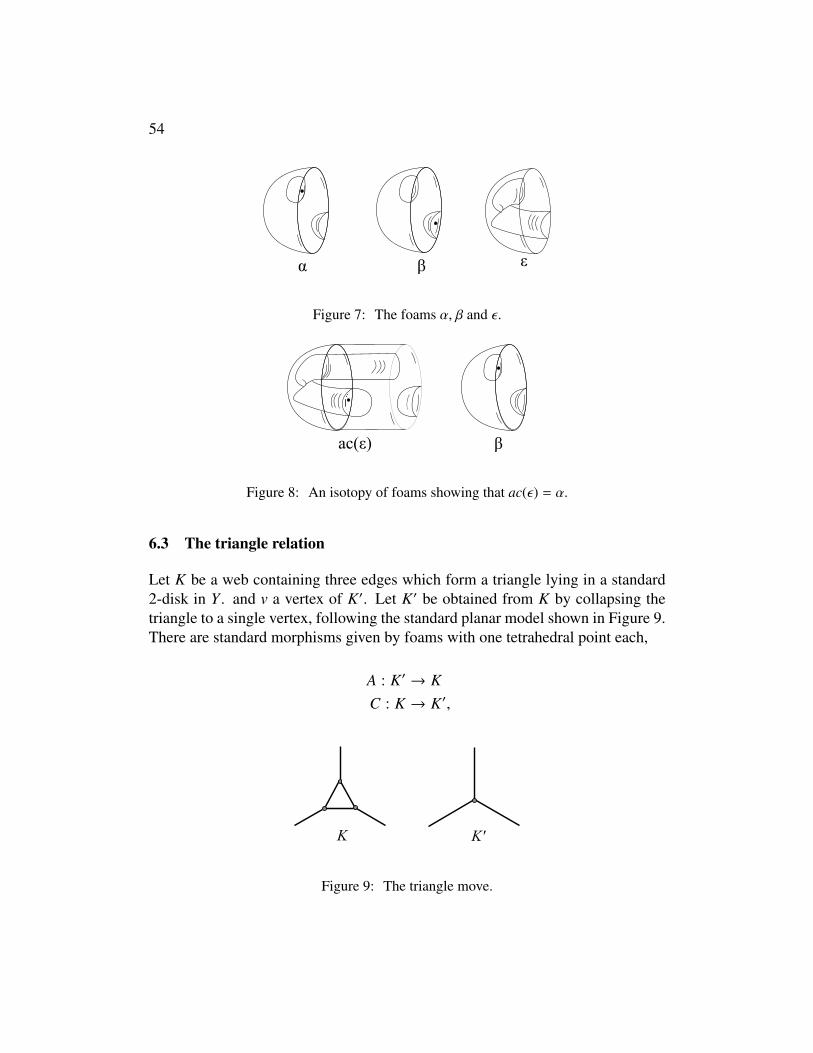
54
α β ε
Figure 7: The foams α, β and ε.
ac(ε) β
Figure 8: An isotopy of foams showing that ac(ε) = α.
6.3 The triangle relation
Let K be a web containing three edges which form a triangle lying in a standard2-disk in Y . and v a vertex of K′. Let K′ be obtained from K by collapsing thetriangle to a single vertex, following the standard planar model shown in Figure 9.There are standard morphisms given by foams with one tetrahedral point each,
A : K′ → KC : K → K′,
Figure 9: The triangle move.
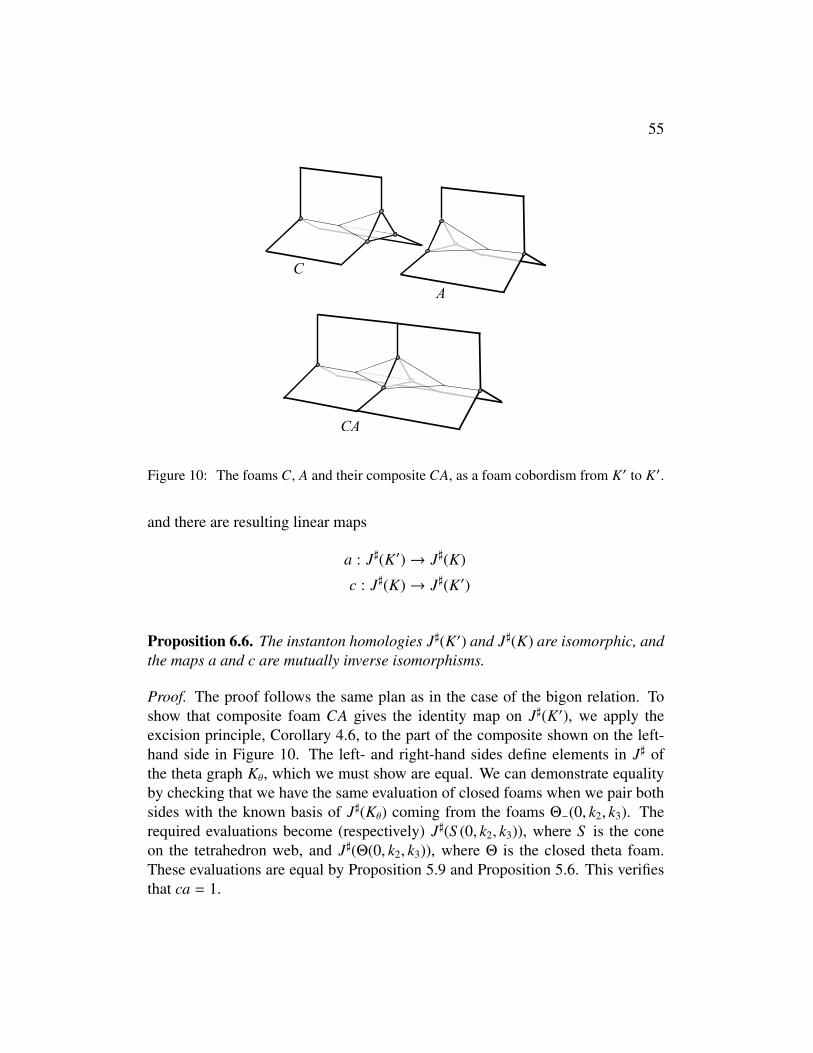
55
Figure 10: The foams C, A and their composite CA, as a foam cobordism from K′ to K′.
and there are resulting linear maps
a : J](K′)→ J](K)
c : J](K)→ J](K′)
Proposition 6.6. The instanton homologies J](K′) and J](K) are isomorphic, andthe maps a and c are mutually inverse isomorphisms.
Proof. The proof follows the same plan as in the case of the bigon relation. Toshow that composite foam CA gives the identity map on J](K′), we apply theexcision principle, Corollary 4.6, to the part of the composite shown on the left-hand side in Figure 10. The left- and right-hand sides define elements in J] ofthe theta graph Kθ, which we must show are equal. We can demonstrate equalityby checking that we have the same evaluation of closed foams when we pair bothsides with the known basis of J](Kθ) coming from the foams Θ−(0, k2, k3). Therequired evaluations become (respectively) J](S (0, k2, k3)), where S is the coneon the tetrahedron web, and J](Θ(0, k2, k3)), where Θ is the closed theta foam.These evaluations are equal by Proposition 5.9 and Proposition 5.6. This verifiesthat ca = 1.
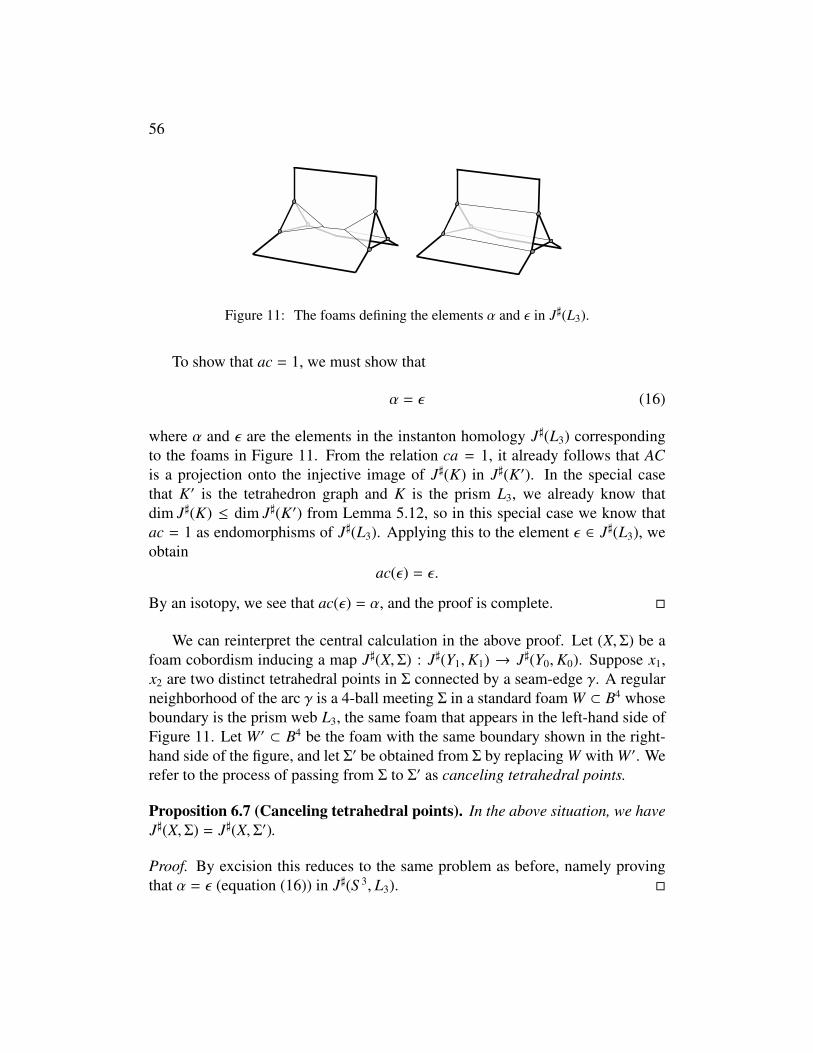
56
Figure 11: The foams defining the elements α and ε in J](L3).
To show that ac = 1, we must show that
α = ε (16)
where α and ε are the elements in the instanton homology J](L3) correspondingto the foams in Figure 11. From the relation ca = 1, it already follows that ACis a projection onto the injective image of J](K) in J](K′). In the special casethat K′ is the tetrahedron graph and K is the prism L3, we already know thatdim J](K) ≤ dim J](K′) from Lemma 5.12, so in this special case we know thatac = 1 as endomorphisms of J](L3). Applying this to the element ε ∈ J](L3), weobtain
ac(ε) = ε.
By an isotopy, we see that ac(ε) = α, and the proof is complete. �
We can reinterpret the central calculation in the above proof. Let (X,Σ) be afoam cobordism inducing a map J](X,Σ) : J](Y1,K1) → J](Y0,K0). Suppose x1,x2 are two distinct tetrahedral points in Σ connected by a seam-edge γ. A regularneighborhood of the arc γ is a 4-ball meeting Σ in a standard foam W ⊂ B4 whoseboundary is the prism web L3, the same foam that appears in the left-hand side ofFigure 11. Let W ′ ⊂ B4 be the foam with the same boundary shown in the right-hand side of the figure, and let Σ′ be obtained from Σ by replacing W with W ′. Werefer to the process of passing from Σ to Σ′ as canceling tetrahedral points.
Proposition 6.7 (Canceling tetrahedral points). In the above situation, we haveJ](X,Σ) = J](X,Σ′).
Proof. By excision this reduces to the same problem as before, namely provingthat α = ε (equation (16)) in J](S 3, L3). �

57
Figure 12: The webs K, K′ and K′′ involved in the square relation: J](K) = J](K′) ⊕J](K′′).
6.4 The square relation
Like the bigon and triangle relations above, our statement and proof of the squarerelation follows [7], with the same sorts of adaptations as in the earlier cases. LetK ⊂ Y be a web containing a square: four edges connecting four vertices in astandard disk. Let K′ and K′′ be obtained from K as shown in Figure 12.
Proposition 6.8. If the web K contains a square and K′, K′′ are as shown inFigure 12, then
J](K) = J](K′) ⊕ J](K′′).
Proof. There are standard morphisms
K′A // KCoo
D // K′′B
oo .
A model for the foam A is shown in Figure 13, and the others are similar. Leta, b, c, d be the corresponding linear maps on J](K′) etc. By an application ofneck-cutting and bubble-bursting, one sees that ca = 1, and similarly db = 1. Byan application of bubble-bursting, one sees that da = 0, and similarly cb = 0. Itfollows ac + bd is a projection onto the injective image of J](K′)⊕ J](K′′), and tocomplete the proof we must show
ac + bd = 1.
In the case that K is a cube, we know that J](K) has dimension at most 24 byLemma 5.12. The webs K′ and K′′ in that case are the same, and can both bereduced to the theta web by the collapsing of a bigon; so J](K′) and J](K′′) bothhave rank 12. So we learn that ac+bd = 1 in the case that K is a cube. The generalcase is now proved by the same strategy as in the bigon and triangle relations. �
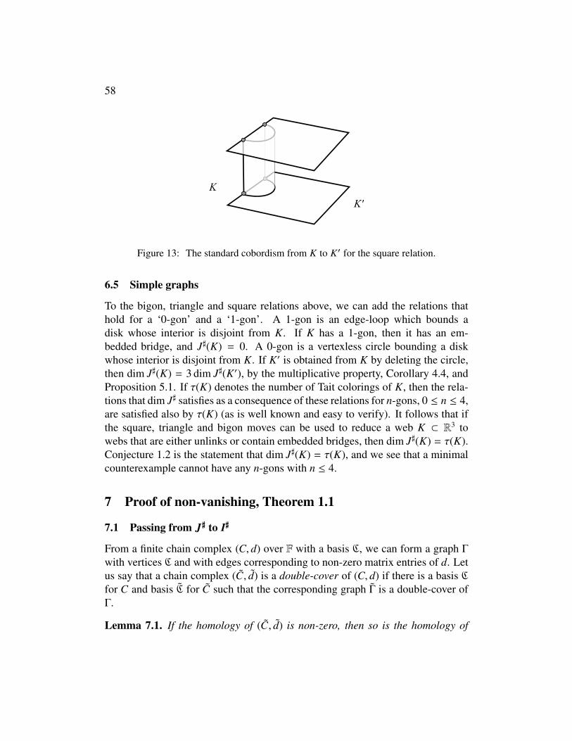
58
Figure 13: The standard cobordism from K to K′ for the square relation.
6.5 Simple graphs
To the bigon, triangle and square relations above, we can add the relations thathold for a ‘0-gon’ and a ‘1-gon’. A 1-gon is an edge-loop which bounds adisk whose interior is disjoint from K. If K has a 1-gon, then it has an em-bedded bridge, and J](K) = 0. A 0-gon is a vertexless circle bounding a diskwhose interior is disjoint from K. If K′ is obtained from K by deleting the circle,then dim J](K) = 3 dim J](K′), by the multiplicative property, Corollary 4.4, andProposition 5.1. If τ(K) denotes the number of Tait colorings of K, then the rela-tions that dim J] satisfies as a consequence of these relations for n-gons, 0 ≤ n ≤ 4,are satisfied also by τ(K) (as is well known and easy to verify). It follows that ifthe square, triangle and bigon moves can be used to reduce a web K ⊂ R3 towebs that are either unlinks or contain embedded bridges, then dim J](K) = τ(K).Conjecture 1.2 is the statement that dim J](K) = τ(K), and we see that a minimalcounterexample cannot have any n-gons with n ≤ 4.
7 Proof of non-vanishing, Theorem 1.1
7.1 Passing from J] to I]
From a finite chain complex (C, d) over F with a basis C, we can form a graph Γ
with vertices C and with edges corresponding to non-zero matrix entries of d. Letus say that a chain complex (C, d) is a double-cover of (C, d) if there is a basis Cfor C and basis C for C such that the corresponding graph Γ is a double-cover ofΓ.
Lemma 7.1. If the homology of (C, d) is non-zero, then so is the homology of
59
(C, d).
Proof. This is a corollary of the standard mod 2 Gysin sequence for the doublecover, i.e. the long exact sequence corresponding to the short exact sequence ofchain complexes
0→ C → C → C → 0.
On the bases C and C, the first map sends a basis element to the sum of its twopreimages, and the second map is the projection. �
If we have a Morse function f on a compact Riemannian manifold B, sat-isfying the Morse-Smale condition, and if we pull it back to a double-cover B,then the pull-back will still be Morse-Smale. Furthermore, the associated Morsecomplex (C, d) will be a double-cover of (C, d) in the above sense. The same ap-plies equally to a Morse complex of the perturbed Chern-Simons functional onBl(Y; µ). This gives us the following result.
Lemma 7.2. Let Y be a bifold with singular set K, and suppose we have twodifferent strong marking data, µ and µ′, with Uµ ⊂ Uµ′ and Eµ = Eµ′ |Uµ\K . SupposeJ(Y; µ′) is non-zero. Then J(Y; µ) is also non-zero.
Proof. According to Lemma 2.4, the map Bl(Y; µ′) → Bl(Y; µ) is an iterateddouble-covering of some union of components of the latter. It follows that the cor-responding chain complex (C′, d′) is an iterated double-cover of some direct sum-mand (C0, d0) of the complex (C, d). The previous lemma tells us that H∗(C0, d0)is non-zero. Therefore H∗(C, d) is non-zero too. �
Corollary 7.3. If K is a web in R3 and I](K) is non-zero, then J](K) is also non-zero.
Proof. This follows from the definition of I] and J] (Section 3.6): they are definedusing the same bifold, but I] is defined using a larger marking set. �
Using also the multiplicative property for split webs, Corollary 4.4, we learnthat, in order to prove the non-vanishing theorem, Theorem 1.1, it will suffice toprove the following variant:
Variant 7.4. If K ⊂ R3 is a non-split web with no embedded bridge, then the Fvector space I](K) is non-zero.
At this point in the argument, we can dispense with J].
60
7.2 Removing vertices
As mentioned in Section 3.6, the construction I] is an extension to webs of theinvariant of links (also called I](K)) which was defined in [15]. We now adoptsome of the notation and concepts from [15] to continue the argument.
Let (Y,K) be a 3-manifold with an embedded web, and let µ be marking datain which the subset Uµ is all of Y . In this case, let us represent w2(Eµ) as a the dualclass to a closed 1-dimensional submanifold w ⊂ Y\K, consisting of a collectionof circles and arcs joining points on edges of K. Since w determines the marking,we may write
Iw(Y,K)
for the invariant that we have previously called J(Y,K; µ). This is the notationused in [15], though we are still using F coefficients. The group is defined only if(Y,K,w) satisfies a condition which is a counterpart of the strong marking condi-tion: a sufficient condition for this is that there is a non-integral surface S in Y:i.e. a closed orientable surface which either
(a) has odd intersection with K, or
(b) is disjoint from K and has odd intersection with w.
See [15, Definition 3.1]. The first condition holds, in particular, if K has a vertex.In this notation, if H ⊂ S 3 is a Hopf link near infinity in S 3 and u is an arc joiningits two components, then for a web K ⊂ R3, we have
I](K) = Iu(S 3,K ∪ H). (17)
There is another notation used in [15, Section 5.2] that we also need to adopthere. On Y , the obstruction to lifting an SO(3) gauge transformation u to thedeterminant-1 gauge group is an element o(u) in H1(Y;F). So the usual config-uration space of connections (the quotient by the determinant-1 gauge group) isacted on by H1(Y;F). Given a choice of subgroup φ ⊂ H1(Y;F), we can formthe quotient of the configuration space by φ and compute the Morse theory of theperturbed Chern-Simons functional on this quotient. The resulting group
Iw(Y,K)φ
is defined whenever φ acts freely on the set of critical points. A sufficient conditionof this is that there be a non-integral surface S such that the restriction of φ to S iszero. (See [15] once more.) In our applications, this condition will always be easy
61
to verify, because there will be a 2-sphere meeting K in three points, on which φwill be zero.
We return to a general (Y,K), with the marking data now represented by w asabove. Let v1, v2 be two vertices of K, and let B1, B2 be standard ball neighbor-hoods of these, each meeting K in three arcs joined at the vertex, disjoint from w.Let Y+ be the oriented 3-manifold obtained by removing the balls Bi and identi-fying the two S 2 boundary components. (Topologically this is Y#(S 1 × S 2).) Wemake the identification so that the three points on ∂B1 where K meets ∂(Y\B1) areidentified (in any order) with the corresponding points on ∂B2. In this way weobtain a new pair (Y+K+), though not uniquely. Because it is disjoint from theballs, we may regard w as a submanifold also of Y+.
Proposition 7.5. In the above situation, if Iw(Y+,K+) is non-zero, then so too isIw(Y,K).
Proof. This is an application of excision. Let S 1 and S 2 be the spheres with threemarked points, ∂B1 and ∂B2. If we cut (Y,K) along S 1 and S 2 and re-glue, thenwe obtain a disconnected manifold with two components:
(Y ′,K′) = (Y+,K+) ∪ (S 3,Θ).
Here Θ is a standard Theta graph in S 3. Let S ⊂ Y+ be the new 2-sphere wherethe two surfaces are identified. Combing the argument of [15, Theorem 5.6] withTheorem 4.2, there is an excision isomorphism,
Iw(Y,K) � Iw(Y ′,K′)ψ
= Iw(Y+,K+)ψ ⊗ I(S 3,Θ),
where the subgroup ψ ⊂ H1(Y ′;F) is the 2-element subgroup generated by theclass dual to S .
Since the I(S 3,Θ) = F, we see that non-vanishing of Iw(Y,K) is equivalent tonon-vanishing of Iw(Y+,K+)ψ. By the double-cover argument of Section 7.1, thisis implied by the non-vanishing of Iw(Y+,K+). �
If K ⊂ S 3 is a web, let 2n be the number of vertices (which is always even).We may pair these up arbitrarily, and apply the above topological construction ntimes to obtain a new pair (Y+,K+) with no vertices at all. The manifold Y+ willbe a connected sum of n copies of S 1 × S 2. We call this process excising all thevertices.
62
7.3 A taut sutured manifold
Let us turn again to the situation of Proposition 7.4. In the notation (17), we arelooking at Iu(S 3,K ∪ H). Excising all the vertices and applying Proposition 7.5,we see that it suffices to prove the following variant:
Variant 7.6. Suppose K ⊂ S 3 is a non-split web without an embedded bridge andlet H and u be as before. Let (Y+,K+) be obtained from (S 3,K) be excising all thevertices. Then Iu(Y+,K+ ∪ H) is non-zero.
Our next step deals with the Hopf link H. We state a lemma which involvessumming a Hopf link onto one of the components of a link K.
Lemma 7.7. Let K ⊂ Y be a web and w ⊂ Y\K a union of arcs representing achoice of w2. Let H and u be a Hopf link and arc as usual, contained in a balldisjoint from K. Let m be a meridian of some edge e of K, i.e. the boundary ofa disk transverse to e, and let v be an arc joining m to e in the disk. Then (withcoefficients still F)), we have
dim Iw+u(Y,K ∪ H) = 2 dim Iw+v(Y,K ∪ m).
Proof. We shall compare both the left- and right-hand sides of the equation to thedimension of the instanton homology when both m and H are included,
Iw+v+u(Y,K ∪ m ∪ H).
The skein exact sequence of [15] gives an exact triangle
· · ·∂→ Iw+u(Y,K ∪ H)→ Iw+v+u(Y,K ∪ m ∪ H)→ Iw+u(Y,K ∪ H)
∂→ . . . .
In the special case that K is the unknot in S 3 and w is empty, we know thatIw+v(Y,K ∪ H) has dimension 2, and Iw+v+u(Y,K ∪ ∪m ∪ H) has dimension 4;so in this case the connecting homomorphism
Iw+u(Y,K ∪ H)∂→ Iw+u(Y,K ∪ H)
is zero (with F coefficients). By an application of Corollary 4.6 it follows that∂ = 0 for all K and w, and hence
dim Iw+v+u(Y,K ∪ m ∪ H) = 2 dim Iw+u(Y,K ∪ H).

63
On the other hand we also have
dim Iw+v+u(Y,K ∪ m ∪ H) = 4 dim Iw+u(Y,K ∪ m). (18)
To see this we can take the disjoint union of Y with a 3-sphere containing twoHopf links,
(Y,K ∪ m) q (S 3,H1 ∪ H2),
and apply the excision principle, cutting and along tori to see that the instantonFloer homology of this union is the same as that of
(Y,K ∪ m ∪ H) q (S 3,H).
The formula (18) then follows from the fact that
dim Iu1+u2(S 3,H1 ∪ ∪H2) = 4 dim Iu(S 3,H).
�
In the situation described in Variant 7.6, let r be the number of components ofthe link K+. (This number will depend on how we chose to make the identifica-tions when we excised all the vertices.) To prove non-vanishing of Iu(Y+,K+∪H),it will suffice to prove non-vanishing of
Iu1+···+ur (Y+,K+ ∪ H1 ∪ · · · ∪ Hr)
because of the tensor product rule for I] of disjoint unions. By the Lemma above,the rank of this group is 2r times the rank of the group
Iv(Y+,K+ ∪ m)
where m = m1 ∪ · · · ∪ mr is a collection of meridians, one for each component ofK+, and v = v1 + · · ·+vr is a collection of standard arcs. We arrive at the followingvariant which is sufficient to prove Theorem 1.1.
Variant 7.8. Let the web K ⊂ S 3 be non-split and without an embedded bridge, let(Y+,K+) be obtained by excising all the vertices, let m be a collection of meridiansof K+, one for each edge, and let v be a collection of standard arcs joining eachmeridian to the corresponding component. Then
Iv(Y+,K+ ∪ m)
is non-zero.
64
If K+ has only one component, then Iv(Y+,K+ ∪m) is exactly the group calledI\(Y+,K+) in [15], though over F here. It is in fact possible to choose the identi-fications when excising the vertices so that r = 1, but we will continue withoutmaking any restriction on r.
We now use excision, to remove all the components of K+ and m, in the sameway that was done for the case r = 1 in [15]. (See in particular [15, Proposi-tion 5.7] for essentially the same argument that we present now.) For each com-ponent K+
i ⊂ K+ and corresponding meridian mi, let T ′i and T ′′i be boundariesof disjoint tubular neighborhoods of K+
i and mi respectively. Let Y+ be the 3-manifold obtained from Y+ be removing all the tubular neighborhoods and gluingT ′i to T ′′i for all i. The gluing is done in such a way that a longitude of K+
i on T ′i isglued to a meridian of mi on T ′′i , and vice versa. In Y+, let Ti be the torus obtainedby the identification of T ′i and T ′′i . We arrange the arc vi, for each i, so that eachhits both T ′i and T ′′i in one point, so that Y+ contains closed curves vi transverse toeach Ti. Let φ be the subgroup of H1(Y+;F) generated by the classes dual to the rtori Ti. By excision argument from the proof of [15, Proposition 5.7], we have anisomorphism
Iv(Y+,K+ ∪ m) � I v(Y+)φ.
(Here v, of course, is the sum of the vi. Note also that there is no link or web Kin Y+.) Applying the double-cover argument again, we see that we will be done ifwe can show that I v(Y+) is non-zero.
At this point, we appeal to the universal coefficient theorem, which tells us thata finite complex over Z has non-trivial homology over F if it has non-zero homol-ogy over Q. So we will aim to prove that I v(Y+;Q) is non-zero. As in Section 5of [15], this last group is essentially the same as the sutured Floer homology ofan associated sutured manifold. To state it precisely, let M be complement in Y+
of a tubular neighborhood of K+. Let (M, γ) be the sutured manifold obtained byputting two meridional sutures on each boundary component. Then we have
dim I v(Y+;Q) = 2 dim SHI(M, γ),
where SHI is the sutured instanton Floer homology from [13]. Our proof will becomplete if we can show that SHI(M, γ) is non-zero. According to [13, Proposi-tion 7.12], the sutured instanton homology is non-zero provided that (M, γ) is tautin the sense of [6]. (The proof of that Proposition rests on the existence of suturedmanifold hierarchies for taut sutured manifolds, proved in [6].) So the followingvariant will suffice:
65
Variant 7.9. Let the web K ⊂ S 3 be non-split and without an embedded bridge,let (Y+,K+) be obtained by excising all the vertices (so Y+ is a connected sum ofn copies of S 1 × S 2), and let (M, γ) be the sutured link complement. Then (M, γ)is taut.
7.4 Proof of tautness
We will now show that (M, γ) is taut. From the definition, this means establishing:
(a) every 2-sphere in M bounds a ball; and
(b) no meridional curve on ∂M bounds a disk.
(The meridional curves are the curves parallel to the sutures.)By its construction, M contains n pairs of pants P1, . . . , Pn, obtained from the
standard 2-spheres in #(S 1 × S 2) by removing the neighborhood of K+. Write Pfor their union. If we cut M along P, we obtain a 3-manifold diffeomorphic tothe complement of a regular neighborhood of K ⊂ S 3. The hypothesis that K isnon-split can therefore be restated as the condition that every 2-sphere in M\Pbounds a ball in M\P. Similarly, the hypothesis that K has no embedded bridgecan be stated as the condition that no meridional curve on (∂M\P) bounds a diskin M\P.
So, for a proof by contradiction, it will suffice to establish the following:
Lemma 7.10. If there is a sphere S ⊂ M contradicting (a), or a disk D ⊂ Mcontradicting (b), then there is another sphere S ′ or disk D′ (not necessarily “re-spectively”) contradicting (a) or (b) with the additional property that it is disjointfrom P.
Proof. Suppose first that D is a disk contradicting (b). We may assume that theboundary of D is disjoint from P and that D meets P transversely in a collectionof disjoint simple closed curves. Assume there is no disk D′ with meridionalboundary disjoint from P. Then the number of curves in D ∩ P is always non-zero, and we can choose D to minimize this number.
Any curve on P either bounds a disk or is parallel to a boundary componentof P. Given any collection of curves C on P, there is always at least one curveamong them that either bounds a disk δ in P disjoint from the other componentsof C, or cobounds with ∂P an annulus α which is disjoint from the other curves inC. Applying this statement to C = D ∩ P, we let γ be a component of D ∩ P thateither bounds a disk δ, or cobounds an annulus α, disjoint from the other curves
66
of intersection. Suppose γ bounds a disk δ. The curve γ also lies on the embeddeddisk D. Let A ⊂ D be the annulus bounded by ∂D and γ. The interior of A mayintersect P, but will do so in a collection of curves that is smaller than D∩P. Fromthe union of A and a parallel push-off of the disk δ (pushed off to be disjoint fromP, on the same side locally as A), we form a new disk D∗ with the same boundaryas D but with fewer curves of intersection with P. This contradicts the choice ofD. In the case that γ cobounds an annulus α ⊂ P, and the interior of α is disjointfrom D, we define A as before and consider the disk formed as the union of α andD\A. Pushing α off P as before, we obtain a disk D∗ with meridional boundaryhaving fewer curves of intersection with P than D did: the same contradiction.
Now suppose there is a sphere S ⊂ M contradicting (a). Suppose that everysphere S ′ in M\P bounds a ball in M\P. Then S must intersect P. Arrange thatS ∩ P is transverse and let C be this collection of curves. If a component γ ⊂ Cis isotopic in P to a boundary curve, then let α ⊂ P be the annulus bounded byγ and the boundary of P. The curve γ cuts S into two disks. The union of oneof these disks with α is an immersed disk in M with meridional boundary. ByDehn’s lemma, there is also an embedded disk D in M, with the same boundary.This takes us back to case (b), which we have already dealt with.
There remains the case that every component of C = S ∩ P bounds a disk inP. Let us choose S so that the number of components of C is as small as possible.Among the components of C, there is a curve γ that bounds a disk δ ⊂ P whichis disjoint from the other curves in C. If we surger S along δ, we obtain twospheres S 1 and S 2. Let C1 and C2 be their curves of intersecton with P. We haveC1 ∪ C2 = C\γ. So, by our minimality hypothesis on S , it follows that both S 1
and S 2 bound balls, B1 and B2 in M. The union of the balls, together with a two-sided collar of δ, is an immersed ball B in M with boundary S . (The ball is onlyimmersed because B1 and B2 may not be disjoint.) An embedded sphere whichbounds an immersed ball also bounds an embedded ball. So S bounds a ball inM, contrary to hypothesis. �
The proof of this lemma completes the proof of Theorem 1.1. It is clear fromthe proof that a more general result holds, which we state here:
Theorem 7.11. Let Y be a closed, oriented 3-manifold and K ⊂ Y an embeddedweb. Suppose that the complement K\Y is irreducible (every 2-sphere bounds aball), and that K has no embedded bridge (no meridian of K bounds a disk in thecomplement). Then J](Y,K) is non-zero.
Proof. From K ⊂ Y , we form (Y+,K+) as before by excising all vertices. So Y+ is
67
the connected sum of Y with n copies of S 1×S 2 and K+ is an r-component link inY+. Let (M, γ) be the sutured link complement, with 2 meridional sutures on eachcomponent of the r components of the boundary. The same sequence of variantsapplies, and we left to show again that (M, γ) is taut. The proof of Lemma 7.10still applies, without change. �
8 Tait-colorings, O(2) representations and other topics
8.1 O(2) connections and Tait colorings of spatial and planar graphs
Let (Y,K) be a connected 3-manifold containing a web K with at least one vertex.As discussed in Section 2.9, an SO(3) bifold connection (E, A) has automorphismgroup Γ(E, A) which is either V4, Z/2 or trivial, according as the correspondingconnection is a V4-connection, a fully O(2)-connection, or a fully irreducible con-nection respectively. We write R(Y,K) for the space of flat bifold connections.
The following lemma is a straightforward observation. (See also Lemma 2.12.)
Lemma 8.1. If K is a planar graph and R(K) contains an O(2) connection, thenR(K) also admits a V4 connection, and K therefore admits a Tait coloring.
Proof. The are two different conjugacy classes of elements of order 2 in O(2).There is the central element, i, and the conjugacy class of “reflections” that com-prise the non-identity component of O(2). If K ⊂ R3 is a (not necessarily planar)web and ρ a fully O(2) connection in R(K), then each edge of K is labeled by anelement that is either a reflection or central. Furthermore, two reflection edgesmeet at each trivalent vertex. The reflection edges therefore form a 2-factor for K(by definition, a set of edges with two edges incident at each vertex). The edgesin the 2-factor form a collection of closed curves.
If the web is planar, then we can give a standard meridian generator for eachedge, by connecting a standard loop to a point above the plane (as one does for theWirtinger presentation of a knot group). For each edge e, we therefore have a well-defined element ρe in O(2). Along the loops formed by the edges of the 2-factor,the elements ρem , ρem+1 corresponding to consecutive edges differ by multiplicationby i. There are therefore an even number of edges in each loop in the 2-factor.There is therefore a Tait coloring of K, in which the edges in the 2-factor arelabeled alternately j and k, and the remaining edges are labeled i. �
From these lemmas, we obtain an elementary reformulation of the four-colortheorem as the statement that, for any bridgeless planar web K, the representationvariety R(K) contains an O(2) connection.
68
For non-planar webs inR3, the existence of an O(2) connection does not implythe existence of a Tait coloring. Nor is it true that, for every web K in R3 withouta spatial bridge, the representation variety R(K) contains on O(2) representation.(An example with no O(2) representation can be constructed by starting with anon-split 2-component L whose two components bound disjoint Seifert surfaces,and taking K to be the union of L with an extra edge joining the two components.)
8.2 Foams with non-zero evaluation, and O(2) connections
The remarks about O(2) representations for webs in the previous subsection aremotivated in part by the following positive result about O(2) bifold connectionsfor foams in 4-manifolds.
Proposition 8.2. Let Σ be a closed foam in a closed 4-manifold X (possibly withdots). If J](X,Σ) is non-zero, then for every Riemannian metric on the correspond-ing bifold X, there exists an anti-self-dual O(2) bifold connection.
Furthermore, if X admits an orientation-reversing diffeomorphism that fixes Σ
pointwise, then there exists a flat O(2) bifold connection.
Proof. First of all, we can immediately reduce to the case of dotless foams byapplying Proposition 6.4.
Let Z be the product S 1 × S 3 containing the foam S 1 × H, where H is theHopf link. Let Z be the corresponding bifold. The non-vanishing of J](X,Σ)implies the existence, for all metrics, of an anti-self-dual SO(3) bifold connectionon the connected sum X#Z. (The connected sum X#Z is the manifold we obtainwhen we regard X as a cobordism from S 3 to S 3 by removing two balls, and thengluing the two boundary components together.) Furthermore, these anti-self-dualconnections lie in 0-dimensional moduli spaces.
By the usual connected sum argument, either X or Z carries a solution ly-ing in a negative-dimensional moduli space. The κ = 0 moduli space on Z hasformal dimension 0, so in fact X must carry an anti-self-dual connection in anegative-dimensional moduli spaces. Furthermore, this must remain true for anyRiemannian metric on X and any small 4-dimensional holonomy perturbation onX. The following lemma therefore completes the proof of the first assertion in theproposition.
Lemma 8.3. If a moduli space on X has negative formal dimension and consistsonly of fully irreducible connections, then a small holonomy perturbation can bechosen so as to make the moduli space empty.

69
Proof. We adapt the argument in [4] to our case of SO(3) connections. The mapψ : SO(3) → so(3) given by A 7→ A − AT is equivariant for the adjoint action ofSO(3), and has the property that if H ⊂ SO(3) is any subgroup that is not containedin a conjugate of O(2) then ψ(H) spans so(3). Using ψ to construct perturbationsas in [4, Section 2(b)], one shows the existence of holonomy perturbation suchthat the moduli space is regular at all fully irreducible solutions. �
To prove the last statement in Proposition 8.2, we note that any O(2) connec-tion determines a flat real line bundle on ξ X \ Σ that has non-trivial holonomy onthe links of some 2-dimensional surface S ⊂ Σ ⊂ X comprised of a some subsetof the facets. The curvature of an anti-self-dual O(2) bifold connection can beinterpreted as an anti-self-dual harmonic 2-form, f ∈ H−(ξ), with values in ξ andlying in certain lattice inH2(ξ). An adaptation of the usual argument for reducibleconnections in instanton moduli spaces shows that, for generic metric, any suchorbifold 2-form is zero unless dimH+(ξ) = 0 and dimH−(ξ) , 0. However,if X has an orientation-reversing diffeomorphism fixing Σ, then these two vectorspaces have the same dimension. �
Corollary 8.4. Let Σ be a closed foam in R3 ⊂ R4. If J](Σ) is non-zero, then thefoam Σ admits a “Tait coloring”: a coloring of the facets of Σ by three colors sothat all three colors appear on the facets incident to each seam.
Proof. By the previous proposition, there is a flat O(2) bifold connection on(R4,Σ). We shall imitate the argument from the 3-dimensional case, Lemma 8.1,to see that the existence of a flat O(2) connection implies the existence of flat V4
connection when Σ is contained in R3.Whether or not Σ is contained in R3, given an O(2) bifold connection and
corresponding homomorphism ρ from π1(X \Σ), a representative of the conjugacyclass corresponding to the link of each facet of Σ in X is mapped by ρ either to thecentral element i in O(2) or to a reflection. The reflection facets constitute whatwe can call a “2-factor” for the foam: a subset of the facets such that, along eachseam, two of the three facets which meet locally there belong to this subset. Thefacets belonging to the 2-factor form a collection of closed surfaces in S ⊂ X.
When Σ is contained in R3, then there is a standard representative in π1(X \ Σ)for the link of each facet, so ρ gives a map from facets to elements of order 2 inO(2), much as in the case of a planar web. So for each facet f , we have an elementρ f . For facets in the 2-factor, ρ f is a reflection, and if two such facets f1 and f2
are separated by a seam then ρ f1 = iρ f2 . On each component of the closed surfaceS , the facets are therefore labeled by only 2 distinct reflections, in a checkerboard
70
fashion. We can therefore give a Tait coloring of the facts by coloring the rotationfacets with i and the refection facets alternately by j and k. �
Corollary 8.5. If Σ is a closed foam in R3 with J](Σ) , 0, then the seams of Σ
form a bipartite 4-valent graph.
Proof. The proof of the previous corollary shows that the seam Γ is a 4-valentgraph lying on a closed surface S ⊂ R3, and that the facets into which S is dividedadmit a coloring with two colors called j and k. For each connected componentS m of S , the corresponding subgraph of Γ is formed as the transverse intersectionof a collection of circles γm,l arising as boundary components of the facets labeledby the central element i ∈ O(2) (i.e. the facets not contained in S ). The surface S m
separates R3 into two components, and we can therefore partition the circles γm,l
into two types, according to the component in which the corresponding facet ofΣ\S lies. Circles γ and γ′ belonging to the same type do not intersect. We can nowdistinguish two different types of intersection points, as follows. After choosingan orientation of S m, we can choose an oriented chart at each intersection pointin S m which maps the circle γ of the first type to the x axis and the circle of thesecond type to the y axis. The first quadrant is then colored by either j or k. Inthis way we partition the vertices of Γ into two sets, in a way that exhibits Γ asbipartite. �
Corollary 8.6. Let Σ ⊂ X be a closed foam in a closed 4-manifold X withJ](X,Σ) , 0. Let K ⊂ Y be the transverse intersection of Σ with a closed 3-manifold Y ⊂ X. Then R(Y,K) contains a flat O(2) connection.
Furthermore, if K is planar, meaning that it is contained in a standard 2-diskin Y. Then K admits a Tait coloring.
Proof. We know from Proposition 8.2 that, for every metric on the bifold X, thereexists an anti-self-dual O(2) connection on X. Furthermore, the action of thisconnection has an upper bound that is independent of the metric. If we choose asequence of metrics on X that contain cylinders on Y of increasing length, thenstandard applications of the compactness theorems will lead to a flat O(2) con-nection on Y . If K is planar, then the O(2) connection leads to a Tait coloring asbefore. �
Because of the previous corollaries, an affirmative answer to the followingquestion would provide a proof of the four-color theorem.
Question 8.7. If K ⊂ R3 is bridgeless and planar, does it arise as R3 ∩Σ for somefoam Σ ⊂ R4 with J](Σ) , 0?

71
In the situation considered by the question above, we can regard the evaluationof J](Σ) as a pairing of an element of J](K) with an element in the dual spaceJ](−K), where −K is the mirror image. Because we know that J](K) is non-trivial,an affirmative answer to the next question would also suffice.
Question 8.8. Let K ⊂ S 3 be a planar web. Is it always true that J](K) is gener-ated by the elements J](Σ) for foams Σ ⊂ (R4)+ with boundary K?
Remarks. If K ⊂ R3 is spatial web that is not planar, it may be that there are noO(2) representations in R(K), as noted previously. For such a K, there cannot befoam Σ with J](Σ) , 0 such Σ ∩ R3 = K. So one cannot expect an affirmativeanswer to either of the two questions above if one drops the planar hypothesis forK.
Whether it is reasonable to conjecture an affirmative answer to this questionfor planar graphs is not at all clear. For example, in the case of the dodecahedralgraph K, an affirmative answer would probably require that the elements J](Σ)corresponding to foams Σ with boundary K span a space of dimension at least 60(since this is the number of Tait colorings). Calculations by the authors failed toshow that the span had dimension any larger than 58.
8.3 A combinatorial counterpart
Motivated by the partial information that we have about the evaluation of closedfoams, we can try to define a purely combinatorial counterpart to J] for planarwebs K, by closely imitating the construction of Khovanov’s sl3 homology from[7]. We shall describe this combinatorial version here, though we do run into aquestion of well-definedness.
Let us consider closed pre-foams, by which we mean abstract 2-dimensionalcell complexes, with finitely many cells, with a local structure modeled on a foam,in the sense defined in this paper. Unlike the pre-foams in [7], no orientations arerequired, and we allow pre-foams to have tetrahedral points. We allow our pre-foams to have decoration by dots.
We can try and define an evaluation, J[(S ) ∈ F, for such prefoams S by apply-ing the following rules.
(a) The seams of the pre-foam form a 4-valent graph. If this graph is not bipar-tite, then we define J[(S ) = 0.
(b) If the seams form a bipartite graph, we can pair up the tetrahedral pointsand cancel them in pairs (Figure 11) to obtain a new pre-foam S ′ with no
72
tetrahedral points. We declare that J[(S ) = J[(S ′), and so reduce to the casethat there are no tetrahedral points.
(c) When there are no tetrahedral points, the seams form a union of circleswhere three facets meet locally. If the monodromy of the three sheets is anon-trivial permutation around any of these circles, then we define J[(S ) =
0. In this way we reduce to the case that the model for the neighborhoodof each component of the seams is a product S 1 × Y , where Y is a standardY-shape graph.
(d) For each component of the seam having a neighborhood of the form S 1×Y ,we apply (abstract) neck-cutting (i.e. surgery) on the three circles parallelto the seam in each of the three neighboring facets, as in [7]. In this waywe reduce to the case that S is a disjoint union of theta-foams and closedsurfaces.
(e) The theta-foams are evaluated using the rule for J] (Proposition 5.6) to leaveonly closed surfaces. The evaluation J[(S ) for a sphere with two dots is 1,for a torus with no dots is 1, and for everything else is zero (including non-orientable components).
The issue of well-definedness arises here because of the choice of how to pairup the tetrahedral points, but the following two conjectures both seem plausible.
Conjecture 8.9. The above rules lead to a unique, well-defined evaluation J[(S ) ∈F for any pre-foam S .
Conjecture 8.10. For a closed foam Σ in R3 with underlying pre-foam S , we haveJ](Σ) = J[(S ).
The difficulty with establishing the second conjecture arises from the fact thatthe abstract surgeries required to do neck-cutting on a pre-foam S may not alwaysbe achieved by embedded surgeries when the pre-foam is embedded as a foam inR3.
Assuming the first of the two conjectures, one can associate an F vector spaceJ[(K) to a planar web K by taking as generators the set of all foams Σ ⊂ (R3)−
with boundary K and relations ∑[Σi] = 0
73
whenever the collection of foams Σi satisfies∑J[(Σi ∪ T ) = 0
for all foams T ⊂ (R3)+ with ∂T = −K. This definition imitates [7]; and byextending the arguments of that paper one can show that J[(K) satisfies the bigon,triangle and square relations. In particular (still contingent on Conjecture 8.9),J[(K) is isomorphic to J](K) at least for simple planar graphs in the sense ofsection 6.5.
If both of the above conjectures are true, then J[(K) is a subquotient of J](K):it is the subspace of J](K) generated by the foams with boundary K, divided bythe annihilator of the dual space generated by the foams with boundary −K.
Remark. Assuming Conjecture 8.9, the authors examined J[(K) in the case of thedodecahedral graph [10], and showed that its dimension in this case is at least 58.See also the remarks at the end of the previous subsection.
8.4 Gradings
Although it plays no real role in the earlier parts of this paper, we consider nowwhether there is a natural Z/d grading on the homology group J](K), or more gen-erally on J(Y,K; µ), for a web K ⊂ Y with strong marking data µ. To formulate thequestion precisely, we write Y as usual for the corresponding bifold, and Bl(Y; µ)for the space of marked bifold connections. For any closed loop ζ inBl(Y; µ) thereis a corresponding spectral flow sfζ; and if sfζ ∈ dZ for all loops ζ, then we canregard J(Y,K; µ) as Z/d graded, in the usual way. With this understood, we havethe following result.
Proposition 8.11. If K ⊂ Y has no vertices, or if the abstract graph underlingK is bipartite, then J(Y,K; µ) may be given a Z/2 grading. If the graph is notbipartite, then in general there may exist closed loops with spectral flow 1, andthere is no non-trivial Z/d grading for any d.
Proof. The spectral flow sfζ is equal to the index d(E, A) for the corresponding4-dimensional bifold connection on S 1 × Y . By the formula 2.6, this in turn isequal to 8κ, where κ is the action of (E, A).
If K has no vertices, then the symbol of the linearized equations with gaugefixing on the bifold S 1 × Y is homotopic to the symbol of a complex-linear op-erator, for we can choose an almost-complex structure on S 1 × Y such that thesubmanifold S 1 × K is almost complex: the appropriate complex-linear operator
74
is then the operator ∂+bar∂∗ coupled to the complexification of E on the complexorbifold. It follows that the real index d(E, A) is even in this case.
In the general case, let e be an edge of K, let me be a meridional circle linkinge, and consider the torus S 1 × me in S 1 × (Y \ K). We can evaluate w2(E) on Te,and we call the result η(e):
η(e) =⟨w2(E), [S 1 × me]
⟩∈ {0, 1}.
If edges e1, e2, e3 meet at a vertex v, then the sum of the meridians [me1] + [me2] +
[me3] is zero in homology, so
η(e1) + η(e2) + η(e3) = 0.
It follows that, at each vertex v, the number edges which are locally incident atv and have η(e) = 1 is either 0 or 2. Let us say that a vertex v of K has Type Iif all incident edges have η(e) = 0, and Type II if two of the incident edges haveη(e) = 1.
Lemma 8.12. If N is the number of vertices of K with Type II, then the action κ isequal to N/8 modulo (1/4)Z.
Proof of the lemma. Let v be any vertex of K, let Bv be a ball neighborhood of v,and consider the restricion of the bifold connection subset S 1×Bv in S 1× Y . Usingradial parallel dilation in the Bv directions, we can alter (E, A) so that the bifoldconnection is flat on S 1 × Bv. The holonomy group of (E, A) on the slice Bv isthe Klein 4-group is V4 = 1, a, b, c. On S 1 × Bv, the flat connection is determinedby the holonomy around four loops: first the three loops which are the meridiansof the three edges in Bv, and fourth the loops S 1 × p for some point p in Bv \ K.After re-ordering the edges, the first three holonomies are a, b and c, while theholonomy around S 1 × p is either 1, a, b or c. If the holonomy around S 1 × p is 1,then v has Type I, otherwise it has Type II.
We see from this description that if v1 and v2 are vertices of the same type(either both Type I or both Type II), then, after modifying the bifold connection alittle, we can find an identification of the neighborhoods
τ : S 1 × Bv1 → S 2 × Bv2
such that the bifold connections (E, A) and τ∗(E, A) are isomorphic on S 1×Bv1 . Wecan then surger (Y,K) by removing the two balls and identifying the boundaries
75
using τ, and we obtain a new bifold connection (E′, A′) for the new pair (Y ′,K′).The new bifold connection has the same action as the original. If the number ofType II vertices is even, then the number of Type I vertices is even also (becauseany web has an even number of vertices in all); so we can then pair up vertices ofthe same type, and apply the above surgery repeatedly to arrive at the case wherethere are no vertices. When there are no vertices, we have already seen that theindex d is even, which means that κ belongs to (1/4)Z.
To complete the proof of the lemma, it is sufficient to exhibit a single exampleof a bifold connection (E, A) on some S 1 × Y whose action is 1/8. So consider thestandard 1-instanton, as an anti-self-dual SO(3)-connection on R × S 3, invariantthe action of S O(4) on S 3. Let Γ ⊂ SO(4) be the group of order 8 generated by thereflections in the coordinate 2-planes of R4. The standard 1-instanton descendsto an anti-self-dual bifold connection (E, A) on R × (S 3/Γ). The bifold Y = S 3/Γcorresponds to the pair (S 3,K), where the web K is the 1-skeleton of a tetrahedron.If we modify the connection to be flat near ±∞, we can glue the two ends to obtaina bifold connection on S 1 × Y with action 1/8. �
We return to the proof of the proposition. Since two edges are incident ateach vertex of Type II in K, the edges e with η(e) = 1 form cycles. If the graphis bipartite, then every cycle contains an even number of vertices, and it followsthat there are an even number of vertices of Type II. By the lemma, the actionis therefore in (1/4)Z in the bipartite case, and so the index d(E, A) is even. Bycontrast, in the non-bipartite case, the example of the tetrahedron web in the proofof the lemma above shows that the action may be 1/8, and the spectral flow sfζaround a closed loop ζ may therefore be 1. �
8.5 The relation between I] and J]
For a web K in R3, we have already considered the relation between I](K) andJ](K) in a very simple form in Corollary 7.3. The essential point in the proof ofthat corollary was the mod-2 Gysin sequence relating the homology of a double-cover to the homology of the base, as a mapping-cone. In the proof of Corol-lary 7.3, passing from J](K) to I](K) involves taking iterated double-covers ofthe spaces of marked bifold connections, so the complex that computes I](K) canbe constructed as an iterated mapping cone. In this section we will describe thecomplex a little more fully, as a “cube”.
Consider first the situation of a finite simplicial complex S with a coveringf : S → S which is the quotient map for an action of the group G = (Z/2)n. We
76
use multiplicative notation for the group. We write F[G] for the group ring of Gover the field F of 2 elements. With coefficients F, we can describe the homologyof S almost tautologically as the homology of the base S with coefficients in alocal system Γ whose stalk is the vector space F[G] at each point. Following [18]we can construct a spectral sequence abutting to this homology group as follows.
The ring F[G] contains an ideal I, the augmentation ideal
I ={∑
g∈G
λgg∣∣∣∣ ∑
g∈G
λg = 0}.
The powers of the augmentation ideal define a filtration {Im} of the group ring.We write Gr for the associated graded:
Gr =⊕
m
Grm
=⊕
m
Im/Im+1.
The dimension of the vector space Grm is(nm
).
For any g ∈ G, the element 1 + g belongs to I, so multiplication by 1 + glowers the filtration level. So multiplication by g induces the identity operator onthe associated graded Gr. The filtration of I of F[G] gives rise to a filtration ofthe local system Γ on S , so there is also an associated graded object Gr∗(Γ). Thelocal system Gr∗(Γ) on S is trivial, because the monodromy elements g ∈ G acttrivially on Gr.
Consider now the cohomology of S with coefficients in Γ. (We choose coho-mology instead of homology for a while, for the sake of the exposition below.)The cochain complex C∗(S ; Γ) has a filtration by subcomplexes C∗(S ;Im) andthere is an associated spectral sequence. The E1 page of the spectral sequenceconsists of the homology groups
H∗(S ; Gr∗(Γ));
and since the local system Gr∗(Γ) is trivial, this is simply
H∗(S ;F) ⊗ Gr∗ � H∗(S ;F) ⊗ F2n.
The individual summands here are
H∗(S ;F) ⊗ Grm � H∗(S ;F) ⊗ F(nm ).
We therefore have:
77
Proposition 8.13 ([18]). There is a spectral sequence whose E1 page is H∗(S ;F)⊗Gr and which abuts to H∗(S ;F).
After selecting a generating set x1, . . . , xn for G, we can unravel the picture alittle further. For any subset A ⊂ {1, . . . , n}, let GA ≤ G be the subgroup generatedby the elements xi with i ∈ A, and let
ξA =∑g∈GA
g ∈ F[G].
As A runs through all subsets, the elements {ξA}A form a basis for F[G]. In thisbasis, the multiplication by xi has the form
xiξA =
ξA, i ∈ A,ξA + ξA∪{i}, i < A.
For a general element of G of the form xI = xi1 xi2 . . . xik (the product of k distinctgenerators), we similarly have
xIξA =∑
A⊂A′⊂A∪I
ξA′ . (19)
In terms of the basis ξA, we can describe the augmentation ideal and its powers by
F m = span{ ξA | |A| ≥ m }.
The formula (19) shows that, when |A| = m,
xIξA = ξA (mod F m+1). (20)
Consider again the local system Γ on S , and regard Γ as having trivializedstalks: so at each vertex of S the stalk is F[G], and to each 1-simplex σ is aassigned multiplication by xI for some I = I(σ). From the filtration {Im} ofF[G], we obtain a filtration of the cochain complex C∗(S ; Γ), as discussed earlier.If we write dΓ for the coboundary operator, we can compare dΓ to the ordinarycoboundary operator d with trivial constant coefficients F[G]. We use the basis ξA
to writeC∗(S ; Γ) =
⊕A
C∗(S ;F)
so thatdΓ =
∑B⊃A
dA,B,
78
where dA,B is the component from the summand indexed by A to the summandindexed by B. For each 1-simplex e and each i ∈ {1, . . . , n} let
ui(e) =
1, i ∈ I(e)0, i < I(e).
These 1-cochains ui on S are cocycles representing the cohomology classes inH1(S ;F) which are the dual basis to the elements xi ∈ G � H1(S ;F). For I =
{i1, . . . ik}, define a cochain UI by
UI(e) = ui1(e)ui2(e) . . . uik(e).
(This could equivalently be written as
UI = ui1 ^1 ui2 ^1 . . . ^1 uik
where ^1 is the reduced product of [20].) From (19), we obtain the formulae
dA,A = d,
and for B ) A,dA,Bα = UB\A ^ α.
If we think of the subsets A as indexing the vertices of a cube, then we have acomplex computing H∗(S ;F) which consists of a copy of C∗(S ;F) at each vertex.In the spectral sequence corresponding to the filtration F m, the E0 page is a directsum of copies of the complex (C∗(S ), d), one at each vertex of the cube. TheE1 page has a copy of H∗(S ;F) at each vertex of the cube and the differentialon E1 is the sum of maps corresponding to edges of the cube: each such map ismultiplication by a class [ui] in H1(S ;F).
To describe essentially the same situation in using Morse homology in thecontext of J] and I], let K ⊂ R3 be a web, let K] = K ∪ H be the web in S 3
obtained by adding a Hopf link H near infinity. Recall that the groups J](K) andI](K) are defined using two different marking data µ and µ′ for bifold connectionson (S 3,K∪H). IfB andB′ denote the corresponding spaces of bifold connections,then there is a map (see Lemma 2.4)
f : B′ → B
which is a covering of a connected component of B. The covering group is thegroup
G = H1(R3\K;F),
79
and the image of f consists of bifold connections (E, A) such that w2(E) is zeroon R3 \ K (regarded as a subset of S 3 \ K])). Because we wish to write the groupG multiplicatively and H1(R3\K;F) additively, we write xh ∈ G for the elementcorresponding to h ∈ H1(R3\K;F). We also write xh for the corresponding linearoperator on F[G], given by translation. The marking data µ ensures in any casethat w2(E) is zero on the sphere are infinity in R3; and if K is connected, thismeans that f is surjective. For connected webs, we are therefore in the situationthat B is the quotient of B′ by the action of G.
At this point, for connected webs K, we can regard I](K) as the Floer homol-ogy of the perturbed Chern-Simons functional on B with coefficients in a localsystem with fiber F[G]. Using the filtration of F[G] by the powers Im of theaugmentation ideal as above, we obtain a filtration of the complex for I](K), andhence a spectral sequence:
Proposition 8.14. For a connected web in R3, there is a spectral sequence whoseE1 page is the vector space
E1 = J](K) ⊗ Gr,
graded by the grading of Gr, and which abuts to I](K).
After choosing a basis for H1(R3\K;F) (i.e. an n-element generating set forG), we can describe the E1 page as a direct sum of 2n copies of J](K), indexed bythe vertices A of a cube of dimension n.
In the Morse theory picture that underlies I], we can describe the total dif-ferential on the E0 page. Let (C](K), d) be the instanton Morse complex whichcomputes J](K), whose basis is the set of critical points of the perturbed Chern-Simons functional on the corresponding space of bifold connections B]. Fix abasis for H1(R3\K;F) (or equivalently a dual basis {γi} in H1(R3\K;F)), so thatthe E0 page of the spectral sequence can be written as a direct sum of 2n copies ofthe complex C](K) indexed by the vertices A of the cube:
E0 =∑
A⊂{1,...,n}
C](K)A.
For each basis element γi, there is a corresponding chain map
ui : C](K)→ C](K).
Its matrix entries can be defined by first choosing a suitable codimension-1 sub-manifold Vi ⊂ B
] representing the corresponding element of H1(B]) and then
80
defining the matrix entry from α to β to be count of index-1 instanton trajectoriesfrom α to β whose intersection with Vi is odd. More generally, for each subsetI ⊂ {1, . . . , n}, there is a map (not a chain map in general),
UI : C](K)→ C](K)
obtained by counting trajectories having odd intersection with Vi for every i ∈ I.(Thus UI = d in the case that I is empty.) The complex that computes I](K) isthen (E0,D) where D has components as follows. For every pair of subsets A ⊂ B,there is a component
DA,B : C](K)B → C](K)A
given DA,B = UB\A.
8.6 Replacing SO(3) by SU(3)
One can construct a variant of J](K) using the group SU(3) in place of SO(3).Given a web K in a 3-manifold Y , form the disjoint union K ∪ H, where H is aHopf link contained in a ball B ⊂ Y Consider (Y,K∪H) as defining a bifold, just asin the SO(3) case. Fix a U(3) bifold bundle with a reduction to SU(3) outside theball B, whose determinant is non-trivial on the periphal torus of the componentsof H. (This non-triviality of the bundle plays the same role as the strong markingdata in the SO(3) case.) The projectively flat connections with fixed determinanton such a bifold bundle correspond to representations
ρ : π1(Y\K, y0)→ SU(3)
satisfying the constraint that, for each edge e of K and any representative me forthe conjugacy class of the meridian of e, the element ρ(me) has order 2 in SU(3).(Compare Definition 2.11.) The SO(3) representation variety R](Y,K) sits insidethe larger SU(3) representation variety as the fixed-point set of complex conjuga-tion acting on the matrix entries.
One can go on to construct the corresponding instanton homology groups,which we temporarily denote by L](K). Unlike the SO(3) case, this can now bedone with integer coefficients. For webs in R3, with F coefficients, it turns out thatthe dimension L](K;F) is equal to the number of Tait colorings of K. In particular,it is independent of the spatial embedding of the web. A proof in the F case can begiven using the ideas of [9]. The same result holds with rational coefficients, butwith a different proof. One can imagine that a Smith-theory argument [19] mightestablish an inequality
dim L](K;F) ≥ dim J](K)
81
for planar webs K, in which case the four-color theorem would follow from The-orem 1.1. However, there is not a version of Smith theory that applies to thesevariants of Floer homology, and one must use the hypothesis of planarity.
References
[1] K. Appel and W. Haken. Every planar map is four colorable, volume 98 of Contem-porary Mathematics. American Mathematical Society, Providence, RI, 1989. Withthe collaboration of J. Koch.
[2] P. J. Braam and S. K. Donaldson. Floer’s work on instanton homology, knots andsurgery. In The Floer memorial volume, volume 133 of Progr. Math., pages 195–256. Birkhauser, Basel, 1995.
[3] S. K. Donaldson. Connections, cohomology and the intersection forms of 4-manifolds. J. Differential Geom., 24(3):275–341, 1986.
[4] S. K. Donaldson. The orientation of Yang-Mills moduli spaces and 4-manifoldtopology. J. Differential Geom., 26(3):397–428, 1987.
[5] A. Floer. Instanton homology, surgery, and knots. In Geometry of low-dimensionalmanifolds, 1 (Durham, 1989), volume 150 of London Math. Soc. Lecture Note Ser.,pages 97–114. Cambridge Univ. Press, Cambridge, 1990.
[6] D. Gabai. Foliations and the topology of 3-manifolds. J. Differential Geom.,18(3):445–503, 1983.
[7] M. Khovanov. sl(3) link homology. Algebr. Geom. Topol., 4:1045–1081, 2004.
[8] P. Kronheimer and T. Mrowka. Monopoles and three-manifolds, volume 10 of NewMathematical Monographs. Cambridge University Press, Cambridge, 2007.
[9] P. B. Kronheimer and T. S. Mrowka. Exact triangles for SO(3) instanton homologyof webs. Preprint, 2015.
[10] P. B. Kronheimer and T. S. Mrowka. Foam calculations for the SO(3) instantonhomology of the dodecahedron. In preparation.
[11] P. B. Kronheimer and T. S. Mrowka. The SO(3) representation variety for the do-decahedral web. In preparation.
[12] P. B. Kronheimer and T. S. Mrowka. Gauge theory for embedded surfaces. I. Topol-ogy, 32(4):773–826, 1993.
82
[13] P. B. Kronheimer and T. S. Mrowka. Knots, sutures, and excision. J. DifferentialGeom., 84(2):301–364, 2010.
[14] P. B. Kronheimer and T. S. Mrowka. Knot homology groups from instantons. J.Topol., 4(4):835–918, 2011.
[15] P. B. Kronheimer and T. S. Mrowka. Khovanov homology is an unknot-detector.Publ. Math. IHES, 113:97–208, 2012.
[16] G. Kuperberg. Spiders for rank 2 Lie algebras. Comm. Math. Phys., 180(1):109–151, 1996.
[17] M. Mackaay, M. Stosic, and P. Vaz. sl(N)-link homology (N ≥ 4) using foams andthe Kapustin-Li formula. Geom. Topol., 13(2):1075–1128, 2009.
[18] S. Papadima and A. I. Suciu. The spectral sequence of an equivariant chain complexand homology with local coefficients. Trans. Amer. Math. Soc., 362(5):2685–2721,2010.
[19] P. A. Smith. Transformations of finite period. Ann. of Math. (2), 39(1):127–164,1938.
[20] N. E. Steenrod. Products of cocycles and extensions of mappings. Ann. of Math.(2), 48:290–320, 1947.
[21] E. J. Street. Towards an instanton floer homology for tangles, 2012. Ph.D. thesis,Harvard University.
[22] P. G. Tait. Listing’s Topologie. Philosophical Magazine (5th Series), 17:30–46,1884.
[23] K. K. Uhlenbeck. Connections with Lp bounds on curvature. Comm. Math. Phys.,83(1):31–42, 1982.