Embed Size (px)
Citation preview
September 29, 2005 17:21 WSPC/139-IJMPA 02519
International Journal of Modern Physics AVol. 20, No. 24 (2005) 5513–5656c© World Scientific Publishing Company
TACHYON DYNAMICS IN OPEN STRING THEORY∗
ASHOKE SEN
Harish-Chandra Research Institute, Chhatnag Road, Jhusi, Allahabad 211019, India
Received 21 February 2005
In this review we describe our current understanding of the properties of open stringtachyons on an unstable D-brane or brane–antibrane system in string theory. The variousstring theoretic methods used for this study include techniques of two-dimensional con-formal field theory, open string field theory, boundary string field theory, noncommuta-tive solitons, etc. We also describe various attempts to understand these results usingfield theoretic methods. These field theory models include toy models like singular poten-tial models and p-adic string theory, as well as more realistic version of the tachyoneffective action based on Dirac–Born–Infeld type action. Finally we study closed stringbackground produced by the “decaying” unstable D-branes, both in the critical stringtheory and in the two-dimensional string theory, and describe the open string com-pleteness conjecture that emerges out of this study. According to this conjecture thequantum dynamics of an unstable D-brane system is described by an internally consis-tent quantum open string field theory without any need to couple the system to closedstrings. Each such system can be regarded as a part of the “hologram” describing thefull string theory.
Keywords: Boundary conformal field theory; open string field theory; tachyon conden-sation; two-dimensional string theory.
Contents
1. Introduction . . . . . . . . . . . . . . . . . . . . . . . . . . . . 55141.1. Motivation . . . . . . . . . . . . . . . . . . . . . . . . . . . . . . . . . 55151.2. Organization of the review . . . . . . . . . . . . . . . . . . . . . . . . 5516
2. Review of Main Results . . . . . . . . . . . . . . . . . . . . . . . 55172.1. Static solutions in superstring theory . . . . . . . . . . . . . . . . . . 55172.2. Time dependent solutions in superstring theory . . . . . . . . . . . . . 55232.3. Static and time dependent solutions in bosonic string theory . . . . . 55252.4. Coupling to closed strings and the open string
completeness conjecture . . . . . . . . . . . . . . . . . . . . . . . . . . 5529
∗Based on lectures given at the 2003 and 2004 ICTP Spring School, TASI 2003, 2003 SummerSchool on Strings, Gravity and Cosmology at Vancouver, 2003 IPM String School at Anzali, Iran,2003 ICTP Latin American School at Sao Paolo, 2004 Nordic meeting at Groningen and 2004Onassis Foundation lecture at Crete.
5513
Int.
J. M
od. P
hys.
A 2
005.
20:5
513-
5656
. Dow
nloa
ded
from
ww
w.w
orld
scie
ntif
ic.c
omby
UN
IVE
RSI
TY
OF
ILL
INO
IS A
T U
RB
AN
A C
HA
MPA
IGN
on
05/1
4/13
. For
per
sona
l use
onl
y.
September 29, 2005 17:21 WSPC/139-IJMPA 02519
5514 A. Sen
3. Conformal Field Theory Methods . . . . . . . . . . . . . . . . . . . 55313.1. Bosonic string theory . . . . . . . . . . . . . . . . . . . . . . . . . . . 55323.2. Superstring theory . . . . . . . . . . . . . . . . . . . . . . . . . . . . . 55373.3. Analysis of the boundary state . . . . . . . . . . . . . . . . . . . . . . 5541
4. Open String Field Theory . . . . . . . . . . . . . . . . . . . . . . 55464.1. First quantized open bosonic string theory . . . . . . . . . . . . . . . 55474.2. Formulation of open bosonic string field theory . . . . . . . . . . . . . 55494.3. Reformulation of the tachyon condensation conjectures in
string field theory . . . . . . . . . . . . . . . . . . . . . . . . . . . . . 55544.4. Verification of the first conjecture . . . . . . . . . . . . . . . . . . . . 55564.5. Verification of the second and third conjectures . . . . . . . . . . . . . 55594.6. Superstring field theory . . . . . . . . . . . . . . . . . . . . . . . . . . 55614.7. Vacuum string field theory . . . . . . . . . . . . . . . . . . . . . . . . 5566
5. Boundary String Field Theory . . . . . . . . . . . . . . . . . . . . 55696. Noncommutative Solitons . . . . . . . . . . . . . . . . . . . . . . 55767. Time Dependent Solutions . . . . . . . . . . . . . . . . . . . . . . 5579
7.1. General procedure . . . . . . . . . . . . . . . . . . . . . . . . . . . . . 55797.2. Specific applications . . . . . . . . . . . . . . . . . . . . . . . . . . . . 5584
8. Effective Action Around the Tachyon Vacuum . . . . . . . . . . . . . 55898.1. Effective action involving the tachyon . . . . . . . . . . . . . . . . . . 55908.2. Classical solutions around the tachyon vacuum . . . . . . . . . . . . . 55928.3. Inclusion of other massless bosonic fields . . . . . . . . . . . . . . . . 55948.4. Supersymmetrization of the effective action . . . . . . . . . . . . . . . 55968.5. Kink solutions of the effective field theory . . . . . . . . . . . . . . . . 5598
9. Toy Models for Tachyon Condensation . . . . . . . . . . . . . . . . . 56009.1. Singular potential model . . . . . . . . . . . . . . . . . . . . . . . . . 56019.2. p-adic string theory . . . . . . . . . . . . . . . . . . . . . . . . . . . . 5602
10. Closed String Emission from “Decaying” D-branes . . . . . . . . . . . 560510.1. Closed string radiation produced by |B1〉 . . . . . . . . . . . . . . . . 560610.2. Closed string fields produced by |B2〉 . . . . . . . . . . . . . . . . . . 5611
11. D0-brane Decay in Two-Dimensional String Theory . . . . . . . . . . . 561211.1. Two-dimensional string theory . . . . . . . . . . . . . . . . . . . . . . 561311.2. D0-brane and its boundary state in two-dimensional string theory . . 561511.3. Closed string background produced by |B1〉 . . . . . . . . . . . . . . . 562011.4. Closed string background produced by |B2〉 . . . . . . . . . . . . . . . 562211.5. Matrix model description of the two-dimensional string theory . . . . 562311.6. D0-brane decay in type 0B string theory . . . . . . . . . . . . . . . . 5629
12. Open String Completeness Conjecture . . . . . . . . . . . . . . . . . 563112.1. Open string completeness in the critical string theory . . . . . . . . . 563112.2. Open string completeness in two-dimensional string theory . . . . . . 563412.3. Generalized holographic principle . . . . . . . . . . . . . . . . . . . . . 5636
Appendix A. Energy–Momentum Tensor from Boundary State . . . . . . . . . . 5637Appendix B. Computation of the Energy of Closed String Radiation from
Unstable D-brane . . . . . . . . . . . . . . . . . . . . . . . . . . . . 5640
1. Introduction
This introductory section is divided into two parts. In Subsec. 1.1 we give a brief
motivation for studying the tachyon dynamics in string theory. Subsection 1.2 sum-
marizes the organization of the paper.
Int.
J. M
od. P
hys.
A 2
005.
20:5
513-
5656
. Dow
nloa
ded
from
ww
w.w
orld
scie
ntif
ic.c
omby
UN
IVE
RSI
TY
OF
ILL
INO
IS A
T U
RB
AN
A C
HA
MPA
IGN
on
05/1
4/13
. For
per
sona
l use
onl
y.
September 29, 2005 17:21 WSPC/139-IJMPA 02519
Tachyon Dynamics in Open String Theory 5515
1.1. Motivation
Historically, a tachyon was defined as a particle that travels faster than light. Using
the relativistic relation v = p√p2+m2
between the velocity v, the spatial momentum
p and massm of a particle we see that for real p a tachyon must have negative mass2.
Clearly neither of these descriptions makes a convincing case for the tachyon.
Quantum field theories offer a much better insight into the role of tachyons. For
this consider a scalar field φ with conventional kinetic term, and a potential V (φ)
which has an extremum at the origin. If we carry out perturbative quantization of
the scalar field by expanding the potential around φ = 0, and ignore the cubic and
higher order terms in the action, we find a particle-like state with mass2 = V ′′(0).
For V ′′(0) positive this describes a particle with positive mass2. But for V ′′(0) < 0
we have a particle with negative mass2, i.e. a tachyon!
In this case however the existence of the tachyon has a clear physical inter-
pretation. For V ′′(0) < 0, the potential V (φ) has a maximum at the origin, and
hence a small displacement of φ away from the origin will make it grow exponentially
in time. Thus perturbation theory, in which we treat the cubic and higher order
terms in the potential to be small, breaks down. From this point of view we see
that the existence of a tachyon in a quantum field theory is associated with an
instability of the system which causes a breakdown of the perturbation theory. This
interpretation also suggests a natural remedy of the problem. We simply need to
expand the potential around a new point in the field space where it has a minimum,
and carry out perturbative quantization of the theory around this point. This in
turn will give a particle with positive mass2 in the spectrum.
Unlike quantum field theories which provide a second quantized description of a
particle, conventional formulation of string theory uses a first quantized formalism.
In this formulation the spectrum of single “particle” states in the theory are
obtained by quantizing the vibrational modes of a single string. Each such state is
characterized by its energy E and momentum p besides other quantum numbers,
and occasionally one finds states for which E2 − p2 < 0. Since E2 − p2 is identified
as the mass2 of a particle, these states correspond to particles of negative mass2,
i.e. tachyons.
The simplest example of such a tachyon appears in the (25 + 1)-dimensional
bosonic string theory. This theory has closed strings as its fundamental excitations,
and the lowest mass2 state of this theory turns out to be tachyonic. One might
suspect that this tachyon may have the same origin as in a quantum field theory,
i.e. we may be carrying out perturbation expansion around an unstable point, and
that the tachyon may be removed once we expand the theory about a stable mini-
mum of the potential. Unfortunately, the first quantized description of string theory
does not allow us to test this hypothesis. In particular, whether the closed string
tachyon potential in the bosonic string theory has a stable minimum still remains
an unsolved problem, and many people believe that this theory is inconsistent due
to the presence of the tachyon in its spectrum. Fortunately various versions of
Int.
J. M
od. P
hys.
A 2
005.
20:5
513-
5656
. Dow
nloa
ded
from
ww
w.w
orld
scie
ntif
ic.c
omby
UN
IVE
RSI
TY
OF
ILL
INO
IS A
T U
RB
AN
A C
HA
MPA
IGN
on
05/1
4/13
. For
per
sona
l use
onl
y.
September 29, 2005 17:21 WSPC/139-IJMPA 02519
5516 A. Sen
superstring theories, defined in 9 + 1 dimensions, have tachyon free closed string
spectrum. These theories are the starting points of most attempts at constructing
a unified theory of nature.
Besides closed strings, some string theories also contain open string excitations
with appropriate boundary conditions at the two ends of the string. According to
our current understanding, open string excitations exist only when we consider a
theory in the presence of soliton like configurations known as D-branes.428,429,265
Conversely, inclusion of open string states in the spectrum implies that we are
quantizing the theory in the presence of a D-brane. To be more specific, a D-p-
brane is a p-dimensional extended object, and in the presence of such a brane lying
along a p-dimensional hypersurface S, the theory contains open string excitations
whose ends are forced to move along the surface S. In the presence of N D-branes
(not necessarily of the same kind) the spectrum contains N 2 different types of open
string, with each end lying on one of the N D-branes. The physical interpretation
of these open string states is that they represent quantum excitations of the system
of D-branes.
It turns out that in some cases the spectrum of open string states on a system
of D-p-branes also contains tachyon. This happens for example on D-p-branes in
bosonic string theory for any p, and D-p-branes in type IIA/IIB superstring theories
for odd/even values of p. Again, from our experience in quantum field theory one
would guess that the existence of the open string tachyons represents an instability
of the D-brane system whose quantum excitations they describe. The natural ques-
tion that arises then is: is there a stable minimum of the tachyon potential around
which we can quantize the theory and get sensible results?
Although our understanding of this subject is still not complete, last several
years have seen much progress in answering this question. These notes are designed
to primarily review the main developments in this subject.
1.2. Organization of the review
This review is organized as follows. In Sec. 2 we give a summary of the main results
reviewed in this paper. In Secs. 3–6 we analyze time independent classical solu-
tions involving the open string tachyon using various techniques. Section 3 uses
the correspondence between two-dimensional conformal field theories and classi-
cal solutions of the equations of motion in open string field theory. Section 4 is
based on direct analysis of the equations of motion of open string field theory. In
Secs. 5 and 6 we discuss application of the methods of boundary string field theory
and noncommutative field theory respectively. In Sec. 7 we construct and analyze
the properties of time dependent solutions involving the tachyon. In Sec. 8 we de-
scribe an effective field theory which reproduces qualitatively some of the results
on time independent and time dependent classical solutions involving the tachyon.
Section 9 is devoted to the discussion of other toy models, e.g. field theories with
singular potential and p-adic string theory, which exhibit some of the features of
Int.
J. M
od. P
hys.
A 2
005.
20:5
513-
5656
. Dow
nloa
ded
from
ww
w.w
orld
scie
ntif
ic.c
omby
UN
IVE
RSI
TY
OF
ILL
INO
IS A
T U
RB
AN
A C
HA
MPA
IGN
on
05/1
4/13
. For
per
sona
l use
onl
y.
September 29, 2005 17:21 WSPC/139-IJMPA 02519
Tachyon Dynamics in Open String Theory 5517
the static solutions involving the open string tachyon. In Sec. 10 we study the effect
of closed string emission from the time dependent rolling tachyon background on
an unstable D-brane. In Sec. 11 we apply the methods discussed in this review to
study the dynamics and decay of an unstable D0-brane in two-dimensional string
theory, and compare these results with exact description of the system using large
N matrix models. Finally in Sec. 12 we propose an open string completeness con-
jecture and generalized holographic principle which explain some of the results of
Secs. 10 and 11.
Throughout this paper we work in the units:
~ = c = α′ = 1 . (1.1)
Thus in this unit the fundamental string tension is (2π)−1. Also our convention for
the space–time metric will be ηµν = diag(−1, 1, . . . , 1).
Before concluding this section we would like to caution the reader that this
review does not cover all aspects of tachyon condensation. For example we do not
address open string tachyon condensation on Dp–Dp′ brane system or branes at
angles.179,228 We also do not review various attempts to find possible cosmological
applications of the open string tachyon;136,77,137,362,190 nor do we address issues
involving closed string tachyon condensation.3 We refer the reader to the original
papers and their citations in spires database for learning these subjects.
Finally we would like to draw the readers’ attention to many other reviews
where different aspects of tachyon condensation have been discussed. A partial list
includes Refs. 47, 459, 163, 227, 399, 195, 520, 521 and 247. For some early studies
in open string tachyon dynamics, see Refs. 35–37.
2. Review of Main Results
In this section we summarize the main results reviewed in this paper. The derivation
of these results will be discussed in the rest of this paper.
2.1. Static solutions in superstring theory
We begin our discussion by reviewing the properties of D-branes in type IIA
and IIB superstring theories. Dp-branes are by definition p-dimensional extended
objects on which fundamental open strings can end. It is well known100,335,427 that
type IIA/IIB string theory contains BPS Dp-branes for even/odd p, and that these
D-branes carry Ramond–Ramond (RR) charges.428 These D-branes are oriented,
and have definite mass per unit p-volume known as tension. The tension of a BPS
Dp-brane in type IIA/IIB string theory is given by
T p = (2π)−pg−1s , (2.1)
where gs is the closed string coupling constant. The BPS D-branes are stable, and
all the open string modes living on such a brane have mass2 ≥ 0. Since these
branes are oriented, given a specific BPS Dp-brane, we shall call a Dp-brane with
Int.
J. M
od. P
hys.
A 2
005.
20:5
513-
5656
. Dow
nloa
ded
from
ww
w.w
orld
scie
ntif
ic.c
omby
UN
IVE
RSI
TY
OF
ILL
INO
IS A
T U
RB
AN
A C
HA
MPA
IGN
on
05/1
4/13
. For
per
sona
l use
onl
y.
September 29, 2005 17:21 WSPC/139-IJMPA 02519
5518 A. Sen
opposite orientation an anti-Dp-brane, or a Dp-brane. The D0-brane in type IIA
string theory also has an antiparticle known as D0-brane, but we cannot describe
it as a D0-brane with reversed orientation.
Although a BPS Dp-brane does not have a negative mass2 (tachyonic) mode,
if we consider a coincident BPS Dp-brane–Dp-brane pair, then the open string
stretched from the brane to the antibrane (or vice versa) has a tachyonic
mode.204,34,205,340,423 This is due to the fact that the GSO projection rule for these
open strings is opposite of that for open strings whose both ends lie on the brane
(or the antibrane). As a result the ground state in the Neveu–Schwarz (NS) sector,
which is normally removed from the spectrum by GSO projection, now becomes
part of the spectrum, giving rise to a tachyonic mode. Altogether there are two
tachyonic modes in the spectrum — one from the open string stretched from the
brane to the antibrane and the other from the open string stretched from the an-
tibrane to the brane. The mass2 of each of these tachyonic modes is given by
m2 = −1
2. (2.2)
Besides the stable BPS Dp-branes, type II string theories also contain in their
spectrum unstable, non-BPS D-branes.463,44,465,466,45 The simplest way to define
these D-branes in IIA/IIB string theory is to begin with a coincident BPS Dp–Dp-
brane pair in type IIB/IIA string theory, and then take an orbifold of the theory by
(−1)FL , where FL denotes the contribution to the space–time fermion number from
the left-moving sector of the worldsheet. Since the RR fields are odd under (−1)FL ,
all the RR fields of type IIB/IIA theory are projected out by the (−1)FL projection.
The twisted sector states then give us back the RR fields of type IIA/IIB theory.
Since (−1)FL reverses the sign of the RR charge, it takes a BPS Dp-brane to a
Dp-brane and vice versa. As a result its action on the open string states on a Dp–
Dp-brane system is to conjugate the Chan–Paton factor by the exchange operator
σ1. Thus modding out the Dp–Dp-brane by (−1)FL removes all open string states
with Chan–Paton factor σ2 and σ3 since these anticommute with σ1, but keeps the
open string states with Chan–Paton factors I and σ1. This gives us a non-BPS
Dp-brane.467
The non-BPS D-branes have precisely those dimensions which BPS D-branes
do not have. Thus type IIA string theory has non-BPS Dp-branes for odd p
and type IIB string theory has non-BPS Dp-branes for even p. These branes are
unoriented and carry a fixed mass per unit p-volume, given by
T p =√
2(2π)−pg−1s . (2.3)
The most important feature that distinguishes the non-BPS D-branes from BPS
D-branes is that the spectrum of open strings on a non-BPS D-brane contains a
single mode of negative mass2 besides infinite number of other modes of mass2 ≥ 0.
This tachyonic mode can be identified as a particular linear combination of the
two tachyons living on the original brane–antibrane pair that survives the (−1)FL
Int.
J. M
od. P
hys.
A 2
005.
20:5
513-
5656
. Dow
nloa
ded
from
ww
w.w
orld
scie
ntif
ic.c
omby
UN
IVE
RSI
TY
OF
ILL
INO
IS A
T U
RB
AN
A C
HA
MPA
IGN
on
05/1
4/13
. For
per
sona
l use
onl
y.
September 29, 2005 17:21 WSPC/139-IJMPA 02519
Tachyon Dynamics in Open String Theory 5519
projection, and has the same mass2 as given in (2.2). Another important feature
that distinguishes a BPS Dp-brane from a non-BPS Dp-brane is that unlike a BPS
Dp-brane which is charged under the RR (p+ 1)-form gauge field of string theory,
a non-BPS D-brane is neutral under these gauge fields. Various other properties of
non-BPS D-branes have been reviewed in Refs. 469, 336 and 47.
Our main goal will be to understand the dynamics of these tachyonic modes.
This however is not a simple task. The dynamics of open strings living on a Dp-
brane is described by a (p+ 1)-dimensional (string) field theory, defined such that
the free field quantization of the field theory reproduces the spectrum of open strings
on the Dp-brane, and the S-matrix elements computed from this field theory repro-
duce the S-matrix elements of open string theory on the D-brane. On a non-BPS
D-brane the existence of a single scalar tachyonic mode shows that the correspond-
ing open string field theory must contain a real scalar field T with mass2 = − 12 ,
whereas the same reasoning shows that open string field theory associated with a co-
incident brane–antibrane system must contain two real scalar fields, or equivalently
one complex scalar field T of mass2 = − 12 . However these fields have nontrivial cou-
pling to all the infinite number of other fields in open string field theory, and hence
one cannot study the dynamics of these tachyonic modes in isolation. Furthermore
since the |mass2| of the tachyonic modes is of the same order of magnitude as that
of the other heavy modes of the string, one cannot work with a simple low energy
effective action obtained by integrating out the other heavy modes of the string.
This is what makes the analysis of the tachyon dynamics nontrivial. Nevertheless,
it is convenient to state the results of the analysis in terms of an effective action
Seff(T, . . .) obtained by formally integrating out all the positive mass2 fields. This
is what we shall do.a Here . . . stands for all the massless bosonic fields, which in the
case of non-BPS Dp-branes include one gauge field and (9−p) scalar fields associated
with the transverse coordinates. For Dp–Dp brane pair the massless fields consist
of two U(1) gauge fields and 2(9 − p) transverse scalar fields.
First we shall state two properties of Seff(T, . . .) which are trivially derived from
the analysis of the tree level S-matrix:
(1) For a non-BPS D-brane the tachyon effective action has a Z2 symmetry under
T → −T , whereas for a brane–antibrane system the tachyon effective action
has a phase symmetry under T → eiαT .
(2) Let V (T ) denote the tachyon effective potential, defined such that for space–
time independent field configuration, and with all the massless fields set to zero,
the tachyon effective action Seff has the form
−∫
dp+1xV (T ) . (2.4)
aAt this stage we would like to remind the reader that our analysis will be only at the level ofclassical open string field theory, and hence integrating out the heavy fields simply amounts toeliminating them by their equations of motion.
Int.
J. M
od. P
hys.
A 2
005.
20:5
513-
5656
. Dow
nloa
ded
from
ww
w.w
orld
scie
ntif
ic.c
omby
UN
IVE
RSI
TY
OF
ILL
INO
IS A
T U
RB
AN
A C
HA
MPA
IGN
on
05/1
4/13
. For
per
sona
l use
onl
y.
September 29, 2005 17:21 WSPC/139-IJMPA 02519
5520 A. Sen
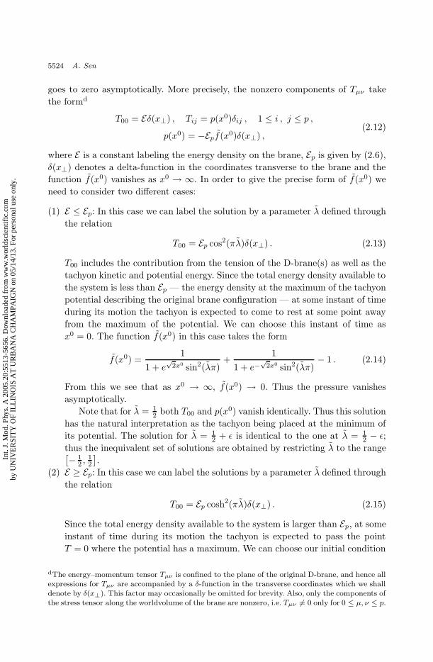
T
p
0
V
T
E
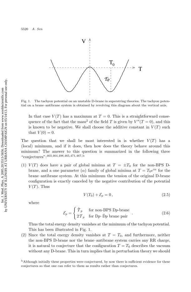
Fig. 1. The tachyon potential on an unstable D-brane in superstring theories. The tachyon poten-tial on a brane–antibrane system is obtained by revolving this diagram about the vertical axis.
In that case V (T ) has a maximum at T = 0. This is a straightforward conse-
quence of the fact that the mass2 of the field T is given by V ′′(T = 0), and this
is known to be negative. We shall choose the additive constant in V (T ) such
that V (0) = 0.
The question that we shall be most interested in is whether V (T ) has a
(local) minimum, and if it does, then how does the theory behave around this
minimum? The answer to this question is summarized in the following three
“conjectures”:463,464,498,465,471,467,b
(1) V (T ) does have a pair of global minima at T = ±T0 for the non-BPS D-
brane, and a one parameter (α) family of global minima at T = T0eiα for the
brane–antibrane system. At this minimum the tension of the original D-brane
configuration is exactly canceled by the negative contribution of the potential
V (T ). Thus
V (T0) + Ep = 0 , (2.5)
where
Ep =
T p for non-BPS Dp-brane
2T p for Dp–Dp brane pair. (2.6)
Thus the total energy density vanishes at the minimum of the tachyon potential.
This has been illustrated in Fig. 1.
(2) Since the total energy density vanishes at T = T0, and furthermore, neither
the non-BPS D-brane nor the brane–antibrane system carries any RR charge,
it is natural to conjecture that the configuration T = T0 describes the vacuum
without any D-brane. This in turn implies that in perturbation theory we should
bAlthough initially these properties were conjectured, by now there is sufficient evidence for theseconjectures so that one can refer to them as results rather than conjectures.
Int.
J. M
od. P
hys.
A 2
005.
20:5
513-
5656
. Dow
nloa
ded
from
ww
w.w
orld
scie
ntif
ic.c
omby
UN
IVE
RSI
TY
OF
ILL
INO
IS A
T U
RB
AN
A C
HA
MPA
IGN
on
05/1
4/13
. For
per
sona
l use
onl
y.
September 29, 2005 17:21 WSPC/139-IJMPA 02519
Tachyon Dynamics in Open String Theory 5521
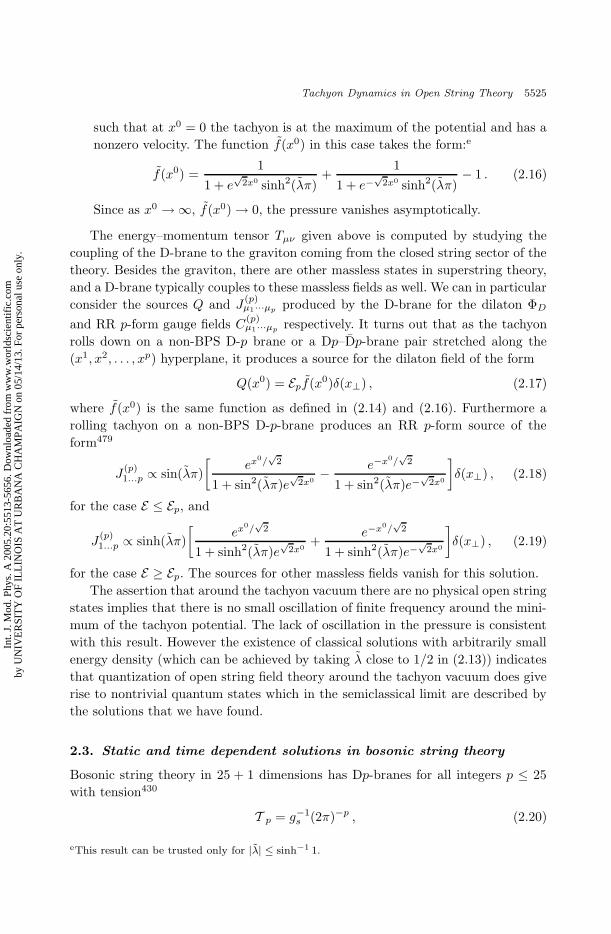
T
−T
0
0
T
px
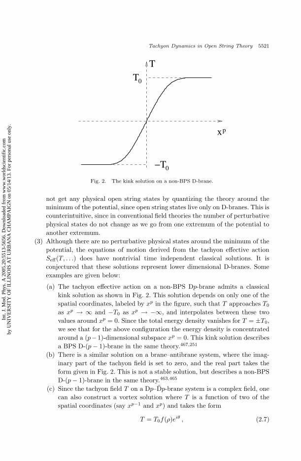
Fig. 2. The kink solution on a non-BPS D-brane.
not get any physical open string states by quantizing the theory around the
minimum of the potential, since open string states live only on D-branes. This is
counterintuitive, since in conventional field theories the number of perturbative
physical states do not change as we go from one extremum of the potential to
another extremum.
(3) Although there are no perturbative physical states around the minimum of the
potential, the equations of motion derived from the tachyon effective action
Seff(T, . . .) does have nontrivial time independent classical solutions. It is
conjectured that these solutions represent lower dimensional D-branes. Some
examples are given below:
(a) The tachyon effective action on a non-BPS Dp-brane admits a classical
kink solution as shown in Fig. 2. This solution depends on only one of the
spatial coordinates, labeled by xp in the figure, such that T approaches T0
as xp → ∞ and −T0 as xp → −∞, and interpolates between these two
values around xp = 0. Since the total energy density vanishes for T = ±T0,
we see that for the above configuration the energy density is concentrated
around a (p−1)-dimensional subspace xp = 0. This kink solution describes
a BPS D-(p− 1)-brane in the same theory.467,251
(b) There is a similar solution on a brane–antibrane system, where the imag-
inary part of the tachyon field is set to zero, and the real part takes the
form given in Fig. 2. This is not a stable solution, but describes a non-BPS
D-(p− 1)-brane in the same theory.463,465
(c) Since the tachyon field T on a Dp–Dp-brane system is a complex field, one
can also construct a vortex solution where T is a function of two of the
spatial coordinates (say xp−1 and xp) and takes the form
T = T0f(ρ)eiθ , (2.7)
Int.
J. M
od. P
hys.
A 2
005.
20:5
513-
5656
. Dow
nloa
ded
from
ww
w.w
orld
scie
ntif
ic.c
omby
UN
IVE
RSI
TY
OF
ILL
INO
IS A
T U
RB
AN
A C
HA
MPA
IGN
on
05/1
4/13
. For
per
sona
l use
onl
y.
September 29, 2005 17:21 WSPC/139-IJMPA 02519
5522 A. Sen
where
ρ =√
(xp−1)2 + (xp)2 , θ = tan−1(xp/xp−1) , (2.8)
are the polar coordinates on the xp−1-xp plane and the function f(ρ) has
the property
f(∞) = 1 , f(0) = 0 . (2.9)
Thus the potential energy associated with the solution vanishes as ρ→ ∞.
Besides the tachyon the solution also contains an accompanying background
gauge field which makes the covariant derivative of the tachyon fall off
sufficiently fast for large ρ so that the net energy density is concentrated
around the ρ = 0 region. This gives a codimension two soliton solution.
This solution describes a BPS D-(p− 2)-brane in the same theory.465,346
(d) If we take a coincident pair of non-BPS D-branes, then the D-brane effective
field theory around T = 0 contains a U(2) gauge field, and there are four
tachyon states represented by a 2× 2 Hermitian matrix valued scalar field
transforming in the adjoint representation of this gauge group. The (ij)
component of the matrix represents the tachyon in the open string sector
beginning on the ith D-brane and ending on the jth D-brane. A family
of minima of the tachyon potential can be found by beginning with the
configuration T = T0
(
1 0
0 −1
)
which represents the tachyon on the first D-
brane at its minimum T0 and the tachyon on the second D-brane at its
minimum −T0, and then making an SU(2) rotation. This gives a family of
minima of the form T = T0n · ~σ , where n is a unit vector and σi are the
Pauli matrices. At any of these minima of the tachyon potential the SU(2)
part of the gauge group is broken to U(1) by the vacuum expectation value
of the tachyon.
This theory contains a ’t Hooft–Polyakov monopole solution250,431
which depends on three of the spatial coordinates ~x, and for which the
asymptotic form of the tachyon and the SU(2) gauge field strengths F aµν
are given by
T (~x) ' T0~σ · ~x|~x| , F a
ij(~x) ' εaij xa
|~x|3 . (2.10)
The energy density of this solution is concentrated around ~x = 0 and hence
this gives a codimension 3-brane. This solution describes a BPS D-(p− 3)-
brane in the same theory.251,346
(e) If we consider a system of two Dp-branes and two Dp-branes, all along the
same plane, then the D-brane worldvolume theory has an U(2)×U(2) gauge
field, and a 2 × 2 matrix valued complex tachyon field T , transforming in
the (2, 2) representation of the gauge group. The (ij) component of the
matrix represents the tachyon field coming from the open string with ends
on the ith D-brane and the jth D-brane. In this case the minimum of
Int.
J. M
od. P
hys.
A 2
005.
20:5
513-
5656
. Dow
nloa
ded
from
ww
w.w
orld
scie
ntif
ic.c
omby
UN
IVE
RSI
TY
OF
ILL
INO
IS A
T U
RB
AN
A C
HA
MPA
IGN
on
05/1
4/13
. For
per
sona
l use
onl
y.
September 29, 2005 17:21 WSPC/139-IJMPA 02519
Tachyon Dynamics in Open String Theory 5523
the tachyon potential where the 11 component of the tachyon takes value
T0eiα and the 22 component of the tachyon takes value T0e
iβ corresponds
to T = T0
(
eiα 0
0 eiβ
)
. A family of minima may now be found by making
arbitrary U(2) rotations from the left and the right. This gives T = T0U
with U being an arbitrary U(2) matrix.
Let A(1)µ and A
(2)µ denote the gauge fields in the two SU(2) gauge
groups. Then we can construct a codimension 4-brane solution where the
fields depend on four of the spatial coordinates, and have the asymptotic
behavior:
T ' T0U(xp−3, xp−2, xp−1, xp) , A(1)µ ' i∂µUU
−1 , A(2)µ ' 0 , (2.11)
where U is an SU(2) matrix valued function of four spatial coordinates,
corresponding to the identity map (winding number one map) from the
surface S3 at spatial infinity to the SU(2) group manifold. This describes
a BPS D-(p− 4)-brane in the same theory.465,346
Quite generally if we begin with sufficient number of non-BPS D9-branes in
type IIA string theory, or D9–D9-branes in type IIB string theory, we can
describe any lower dimensional D-brane as classical solution in this open string
field theory.541,251,346 This has led to a classification of D-branes using a branch
of mathematics known as K-theory (Refs. 541, 251, 173, 212, 46, 419, 530, 420,
460, 143, 162, 382, 220, 68, 424, 544, 451, 152, 348, 260, 196, 357, 384).
2.2. Time dependent solutions in superstring theory
So far we have only discussed time independent solutions of the tachyon equations
of motion. One could also ask questions about time dependent solutions. In partic-
ular, given that the tachyon potential on a non-BPS Dp-brane or a Dp–Dp pair has
the form given in Fig. 1, one could ask: what happens if we displace the tachyon
from the maximum of the potential and let it roll down towards its minimum?c If
T had been an ordinary scalar field then the answer is simple: the tachyon field T
will simply oscillate about the minimum T of the potential, and in the absence of
any dissipative force (as is the case at the classical level) the oscillation will con-
tinue for ever. The energy density T00 will remain constant during this oscillation,
but other components of the energy–momentum tensor, e.g. the pressure p(x0),
defined through Tij = p(x0)δij for 1 ≤ i, j ≤ p, will oscillate about their average
value. However for the case of the string theory tachyon the answer is different and
somewhat surprising.477,478 It turns out that for the rolling tachyon solution on an
unstable D-brane the energy density on the brane remains constant as in the case of
a usual scalar field, but the pressure, instead of oscillating about an average value,
cFor simplicity in this section we shall only describe spatially homogeneous time dependent solu-tions, but more general solutions which depend on both space and time coordinates can also bestudied.480,328
Int.
J. M
od. P
hys.
A 2
005.
20:5
513-
5656
. Dow
nloa
ded
from
ww
w.w
orld
scie
ntif
ic.c
omby
UN
IVE
RSI
TY
OF
ILL
INO
IS A
T U
RB
AN
A C
HA
MPA
IGN
on
05/1
4/13
. For
per
sona
l use
onl
y.
September 29, 2005 17:21 WSPC/139-IJMPA 02519
5524 A. Sen
goes to zero asymptotically. More precisely, the nonzero components of Tµν take
the formd
T00 = Eδ(x⊥) , Tij = p(x0)δij , 1 ≤ i , j ≤ p ,
p(x0) = −Epf(x0)δ(x⊥) ,(2.12)
where E is a constant labeling the energy density on the brane, Ep is given by (2.6),
δ(x⊥) denotes a delta-function in the coordinates transverse to the brane and the
function f(x0) vanishes as x0 → ∞. In order to give the precise form of f(x0) we
need to consider two different cases:
(1) E ≤ Ep: In this case we can label the solution by a parameter λ defined through
the relation
T00 = Ep cos2(πλ)δ(x⊥) . (2.13)
T00 includes the contribution from the tension of the D-brane(s) as well as the
tachyon kinetic and potential energy. Since the total energy density available to
the system is less than Ep — the energy density at the maximum of the tachyon
potential describing the original brane configuration — at some instant of time
during its motion the tachyon is expected to come to rest at some point away
from the maximum of the potential. We can choose this instant of time as
x0 = 0. The function f(x0) in this case takes the form
f(x0) =1
1 + e√
2x0 sin2(λπ)+
1
1 + e−√
2x0 sin2(λπ)− 1 . (2.14)
From this we see that as x0 → ∞, f(x0) → 0. Thus the pressure vanishes
asymptotically.
Note that for λ = 12 both T00 and p(x0) vanish identically. Thus this solution
has the natural interpretation as the tachyon being placed at the minimum of
its potential. The solution for λ = 12 + ε is identical to the one at λ = 1
2 − ε;
thus the inequivalent set of solutions are obtained by restricting λ to the range[
− 12 ,
12
]
.
(2) E ≥ Ep: In this case we can label the solutions by a parameter λ defined through
the relation
T00 = Ep cosh2(πλ)δ(x⊥) . (2.15)
Since the total energy density available to the system is larger than Ep, at some
instant of time during its motion the tachyon is expected to pass the point
T = 0 where the potential has a maximum. We can choose our initial condition
dThe energy–momentum tensor Tµν is confined to the plane of the original D-brane, and hence allexpressions for Tµν are accompanied by a δ-function in the transverse coordinates which we shalldenote by δ(x⊥). This factor may occasionally be omitted for brevity. Also, only the components ofthe stress tensor along the worldvolume of the brane are nonzero, i.e. Tµν 6= 0 only for 0 ≤ µ, ν ≤ p.
Int.
J. M
od. P
hys.
A 2
005.
20:5
513-
5656
. Dow
nloa
ded
from
ww
w.w
orld
scie
ntif
ic.c
omby
UN
IVE
RSI
TY
OF
ILL
INO
IS A
T U
RB
AN
A C
HA
MPA
IGN
on
05/1
4/13
. For
per
sona
l use
onl
y.
September 29, 2005 17:21 WSPC/139-IJMPA 02519
Tachyon Dynamics in Open String Theory 5525
such that at x0 = 0 the tachyon is at the maximum of the potential and has a
nonzero velocity. The function f(x0) in this case takes the form:e
f(x0) =1
1 + e√
2x0 sinh2(λπ)+
1
1 + e−√
2x0 sinh2(λπ)− 1 . (2.16)
Since as x0 → ∞, f(x0) → 0, the pressure vanishes asymptotically.
The energy–momentum tensor Tµν given above is computed by studying the
coupling of the D-brane to the graviton coming from the closed string sector of the
theory. Besides the graviton, there are other massless states in superstring theory,
and a D-brane typically couples to these massless fields as well. We can in particular
consider the sources Q and J(p)µ1···µp produced by the D-brane for the dilaton ΦD
and RR p-form gauge fields C(p)µ1···µp respectively. It turns out that as the tachyon
rolls down on a non-BPS D-p brane or a Dp–Dp-brane pair stretched along the
(x1, x2, . . . , xp) hyperplane, it produces a source for the dilaton field of the form
Q(x0) = Epf(x0)δ(x⊥) , (2.17)
where f(x0) is the same function as defined in (2.14) and (2.16). Furthermore a
rolling tachyon on a non-BPS D-p-brane produces an RR p-form source of the
form479
J(p)1...p ∝ sin(λπ)
[
ex0/√
2
1 + sin2(λπ)e√
2x0− e−x0/
√2
1 + sin2(λπ)e−√
2x0
]
δ(x⊥) , (2.18)
for the case E ≤ Ep, and
J(p)1...p ∝ sinh(λπ)
[
ex0/√
2
1 + sinh2(λπ)e√
2x0+
e−x0/√
2
1 + sinh2(λπ)e−√
2x0
]
δ(x⊥) , (2.19)
for the case E ≥ Ep. The sources for other massless fields vanish for this solution.
The assertion that around the tachyon vacuum there are no physical open string
states implies that there is no small oscillation of finite frequency around the mini-
mum of the tachyon potential. The lack of oscillation in the pressure is consistent
with this result. However the existence of classical solutions with arbitrarily small
energy density (which can be achieved by taking λ close to 1/2 in (2.13)) indicates
that quantization of open string field theory around the tachyon vacuum does give
rise to nontrivial quantum states which in the semiclassical limit are described by
the solutions that we have found.
2.3. Static and time dependent solutions in bosonic string theory
Bosonic string theory in 25 + 1 dimensions has Dp-branes for all integers p ≤ 25
with tension430
T p = g−1s (2π)−p , (2.20)
eThis result can be trusted only for |λ| ≤ sinh−1 1.
Int.
J. M
od. P
hys.
A 2
005.
20:5
513-
5656
. Dow
nloa
ded
from
ww
w.w
orld
scie
ntif
ic.c
omby
UN
IVE
RSI
TY
OF
ILL
INO
IS A
T U
RB
AN
A C
HA
MPA
IGN
on
05/1
4/13
. For
per
sona
l use
onl
y.
September 29, 2005 17:21 WSPC/139-IJMPA 02519
5526 A. Sen
where gs as usual denotes the closed string coupling constant and we are using
α′ = 1 unit. The spectrum of open strings on each of these D-branes contains a
single tachyonic state with mass2 = −1, besides infinite number of other states of
mass2 ≥ 0. Thus among the infinite number of fields appearing in the string field
theory on a Dp-brane, there is a scalar field T with negative mass2. If as in the
case of superstring theory we denote by Seff(T, . . .) the effective action obtained by
integrating out the fields with positive mass2, and by V (T ) the effective potential for
the tachyon obtained by restricting to space–time independent field configurations
and setting the massless fields to zero, then V (T ) will have a maximum at T = 0.
Thus we can again ask: does the potential V (T ) have a (local) minimum, and if it
does, how does the open string field theory behave around this minimum?
Before we go on to answer these questions, let us recall that bosonic string
theory also has a tachyon in the closed string sector, and hence the theory as
it stands is inconsistent. Thus one might wonder why we should be interested in
studying Dp-branes in bosonic string theory in the first place. The reason for this is
simply that (1) although closed string tachyons make the quantum open string field
theory inconsistent due to appearance of closed strings in open string loop diagrams,
classical open string field theory is not directly affected by the closed string tachyon,
and (2) the classical tachyon dynamics on a bosonic Dp-brane has many features in
common with that on a non-BPS D-brane or a brane–antibrane pair in superstring
theory, and yet it is simpler to study than the corresponding problem in superstring
theory. Thus studying tachyon dynamics on a bosonic D-brane gives us valuable
insight into the more relevant problem in superstring theory.
We now summarize the three conjectures describing the static properties of the
tachyon effective action on a bosonic Dp-brane:468,471
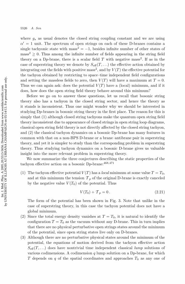
(1) The tachyon effective potential V (T ) has a local minimum at some value T = T0,
and at this minimum the tension T p of the original D-brane is exactly canceled
by the negative value V (T0) of the potential. Thus
V (T0) + T p = 0 . (2.21)
The form of the potential has been shown in Fig. 3. Note that unlike in the
case of superstring theory, in this case the tachyon potential does not have a
global minimum.
(2) Since the total energy density vanishes at T = T0, it is natural to identify the
configuration T = T0 as the vacuum without any D-brane. This in turn implies
that there are no physical perturbative open strings states around the minimum
of the potential, since open string states live only on D-branes.
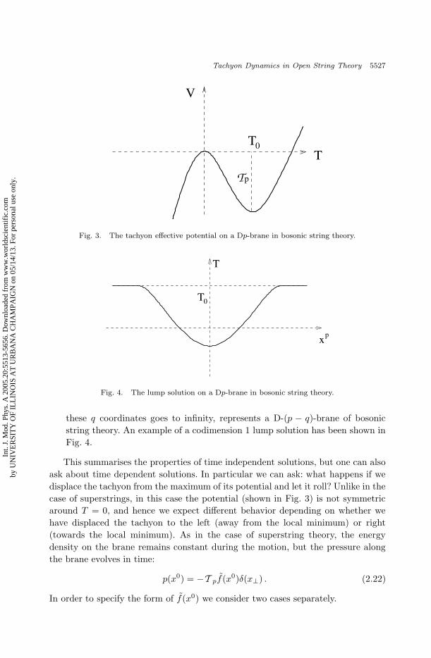
(3) Although there are no perturbative physical states around the minimum of the
potential, the equations of motion derived from the tachyon effective action
Seff(T, . . .) does have nontrivial time independent classical lump solutions of
various codimensions. A codimension q lump solution on a Dp-brane, for which
T depends on q of the spatial coordinates and approaches T0 as any one of
Int.
J. M
od. P
hys.
A 2
005.
20:5
513-
5656
. Dow
nloa
ded
from
ww
w.w
orld
scie
ntif
ic.c
omby
UN
IVE
RSI
TY
OF
ILL
INO
IS A
T U
RB
AN
A C
HA
MPA
IGN
on
05/1
4/13
. For
per
sona
l use
onl
y.
September 29, 2005 17:21 WSPC/139-IJMPA 02519
Tachyon Dynamics in Open String Theory 5527
T
p
0
V
T
T
Fig. 3. The tachyon effective potential on a Dp-brane in bosonic string theory.
0T
T
xp
Fig. 4. The lump solution on a Dp-brane in bosonic string theory.
these q coordinates goes to infinity, represents a D-(p − q)-brane of bosonic
string theory. An example of a codimension 1 lump solution has been shown in
Fig. 4.
This summarises the properties of time independent solutions, but one can also
ask about time dependent solutions. In particular we can ask: what happens if we
displace the tachyon from the maximum of its potential and let it roll? Unlike in the
case of superstrings, in this case the potential (shown in Fig. 3) is not symmetric
around T = 0, and hence we expect different behavior depending on whether we
have displaced the tachyon to the left (away from the local minimum) or right
(towards the local minimum). As in the case of superstring theory, the energy
density on the brane remains constant during the motion, but the pressure along
the brane evolves in time:
p(x0) = −T pf(x0)δ(x⊥) . (2.22)
In order to specify the form of f(x0) we consider two cases separately.
Int.
J. M
od. P
hys.
A 2
005.
20:5
513-
5656
. Dow
nloa
ded
from
ww
w.w
orld
scie
ntif
ic.c
omby
UN
IVE
RSI
TY
OF
ILL
INO
IS A
T U
RB
AN
A C
HA
MPA
IGN
on
05/1
4/13
. For
per
sona
l use
onl
y.
September 29, 2005 17:21 WSPC/139-IJMPA 02519
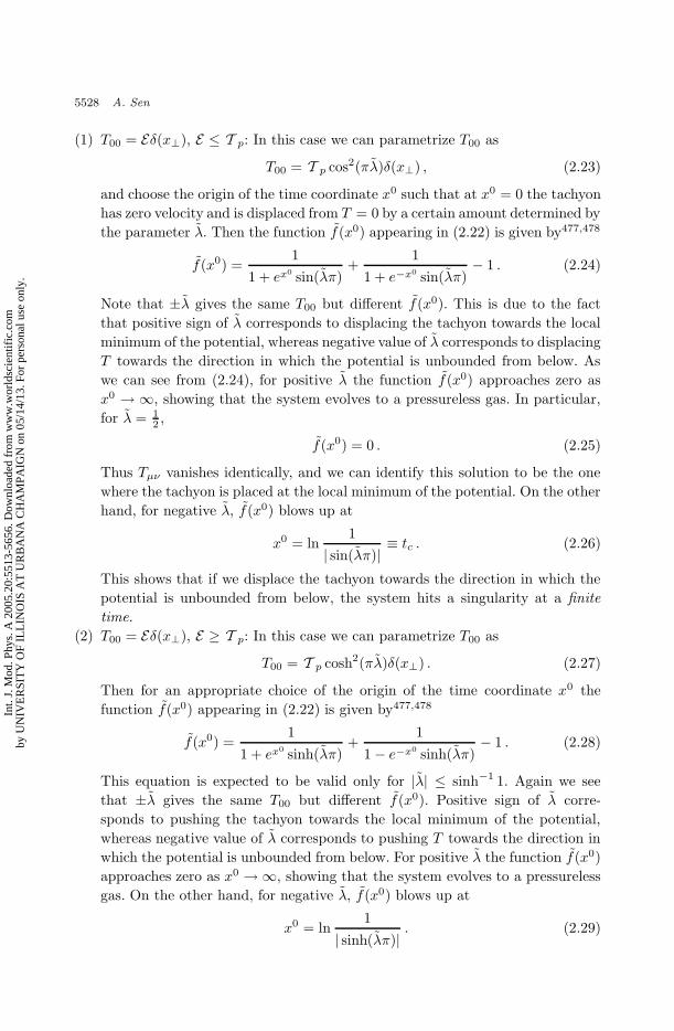
5528 A. Sen
(1) T00 = Eδ(x⊥), E ≤ T p: In this case we can parametrize T00 as
T00 = T p cos2(πλ)δ(x⊥) , (2.23)
and choose the origin of the time coordinate x0 such that at x0 = 0 the tachyon
has zero velocity and is displaced from T = 0 by a certain amount determined by
the parameter λ. Then the function f(x0) appearing in (2.22) is given by477,478
f(x0) =1
1 + ex0 sin(λπ)+
1
1 + e−x0 sin(λπ)− 1 . (2.24)
Note that ±λ gives the same T00 but different f(x0). This is due to the fact
that positive sign of λ corresponds to displacing the tachyon towards the local
minimum of the potential, whereas negative value of λ corresponds to displacing
T towards the direction in which the potential is unbounded from below. As
we can see from (2.24), for positive λ the function f(x0) approaches zero as
x0 → ∞, showing that the system evolves to a pressureless gas. In particular,
for λ = 12 ,
f(x0) = 0 . (2.25)
Thus Tµν vanishes identically, and we can identify this solution to be the one
where the tachyon is placed at the local minimum of the potential. On the other
hand, for negative λ, f(x0) blows up at
x0 = ln1
| sin(λπ)|≡ tc . (2.26)
This shows that if we displace the tachyon towards the direction in which the
potential is unbounded from below, the system hits a singularity at a finite
time.
(2) T00 = Eδ(x⊥), E ≥ T p: In this case we can parametrize T00 as
T00 = T p cosh2(πλ)δ(x⊥) . (2.27)
Then for an appropriate choice of the origin of the time coordinate x0 the
function f(x0) appearing in (2.22) is given by477,478
f(x0) =1
1 + ex0 sinh(λπ)+
1
1 − e−x0 sinh(λπ)− 1 . (2.28)
This equation is expected to be valid only for |λ| ≤ sinh−1 1. Again we see
that ±λ gives the same T00 but different f(x0). Positive sign of λ corre-
sponds to pushing the tachyon towards the local minimum of the potential,
whereas negative value of λ corresponds to pushing T towards the direction in
which the potential is unbounded from below. For positive λ the function f(x0)
approaches zero as x0 → ∞, showing that the system evolves to a pressureless
gas. On the other hand, for negative λ, f(x0) blows up at
x0 = ln1
| sinh(λπ)|. (2.29)
Int.
J. M
od. P
hys.
A 2
005.
20:5
513-
5656
. Dow
nloa
ded
from
ww
w.w
orld
scie
ntif
ic.c
omby
UN
IVE
RSI
TY
OF
ILL
INO
IS A
T U
RB
AN
A C
HA
MPA
IGN
on
05/1
4/13
. For
per
sona
l use
onl
y.
September 29, 2005 17:21 WSPC/139-IJMPA 02519
Tachyon Dynamics in Open String Theory 5529
This again shows that if we displace the tachyon towards the direction in which
the potential is unbounded from below, the system hits a singularity at a finite
time.
Bosonic string theory also has a massless dilaton field and we can define the
dilaton charge density as the source that couples to this field. As in the case of super-
string theory, a rolling tachyon on a D-p-brane of bosonic string theory produces a
source for the dilaton field
Q = T pf(x0)δ(x⊥) , (2.30)
with f(x0) given by Eq. (2.24) or (2.28).
2.4. Coupling to closed strings and the open string
completeness conjecture
So far we have discussed the dynamics of the open string tachyon at the purely
classical level, and have ignored the coupling of the D-brane to closed strings.
Since D-branes act as sources for various closed string fields, a time dependent
open string field configuration such as the rolling tachyon solution acts as a time
dependent source for closed string fields, and produces closed string radiation. This
can be computed using the standard techniques. For unstable Dp-branes with all p
directions wrapped on circles, one finds that the total energy carried by the closed
string radiation is infinite.326,170 However since the initial Dp-brane has finite energy
it is appropriate to regulate this divergence by putting an upper cutoff on the energy
of the emitted closed string. A natural choice of this cutoff is the initial energy of
the D-brane. In that case one finds that
(1) All the energy of the D-brane is radiated away into closed strings even though
any single closed string mode carries a small (∼ gs) fraction of the D-brane
energy.
(2) Most of the energy is carried by closed strings of mass ∼ 1gs
.
(3) The typical momentum carried by these closed strings along directions trans-
verse to the D-brane is of order√
1gs
, and the typical winding charge carried by
these strings along directions tangential to the D-brane is also of order√
1gs
.
From the first result one would tend to conclude that the effect of closed string
emission should invalidate the classical open string results on the rolling tachyon
system discussed earlier. There are however some surprising coincidences:
(1) The tree level open string analysis tell us that the final system associated with
the rolling tachyon configuration has zero pressure. On the other hand closed
string emission results tell us that the final closed strings have momentum/mass
and winding/mass ratio of order√gs and hence pressure/energy density ratio
of order gs. In the gs → 0 limit this vanishes. Thus it appears that the classical
Int.
J. M
od. P
hys.
A 2
005.
20:5
513-
5656
. Dow
nloa
ded
from
ww
w.w
orld
scie
ntif
ic.c
omby
UN
IVE
RSI
TY
OF
ILL
INO
IS A
T U
RB
AN
A C
HA
MPA
IGN
on
05/1
4/13
. For
per
sona
l use
onl
y.
September 29, 2005 17:21 WSPC/139-IJMPA 02519
5530 A. Sen
open string analysis correctly predicts the equation of state of the final system
of closed strings into which the system decays.
(2) The tree level open string analysis tells us that the final system has zero dilaton
charge. By analyzing the properties of the closed string radiation produced by
the decaying D-brane one finds that these closed strings also carry zero dilaton
charge. Thus the classical open string analysis correctly captures the properties
of the final state closed strings produced during the D-brane decay.
These results (together with some generalizations which will be discussed briefly
in Subsec. 12.1) suggest that the classical open string theory already knows about
the properties of the final state closed strings produced by the decay of the D-
brane.483,484 This can be formally stated as an open string completeness conjecture
according to which the complete dynamics of a D-brane is captured by the quantum
open string theory without any need to explicitly consider the coupling of the system
to closed strings.f Closed strings provide a dual description of the system. This does
not imply that any arbitrary state in string theory can be described in terms of
open string theory on an unstable D-brane, but does imply that all the quantum
states required to describe the dynamics of a given D-brane are contained in the
open string theory associated with that D-brane.
At the level of critical string theory one cannot prove this conjecture. How-
ever it turns out that this conjecture has a simple realization in a noncritical two-
dimensional string theory. This theory has two equivalent descriptions: (1) as a
regular string theory in a somewhat complicated background107,125 in which the
worldsheet dynamics of the fundamental string is described by the direct sum of
a free scalar field theory and the Liouville theory with central charge 25, and
(2) as a theory of free nonrelativistic fermions moving under a shifted inverted
harmonic oscillator potential − 12q
2 + 1gs
.207,73,193 Although in the free fermion
description the potential is unbounded from below, the ground state of the system
has all the negative energy states filled, and hence the second quantized theory
is well defined. The map between these two theories is also known. In particular
the closed string states in the first description are related to the quanta of the
scalar field obtained by bosonizing the second quantized fermion field in the second
description.101,491,208
In the regular string theory description the theory also has an unstable D0-brane
with a tachyonic mode.552 The classical properties of this tachyon are identical to
those discussed in Subsec. 2.3 in the context of critical bosonic string theory. In
particular one can construct time dependent solution describing the rolling of the
tachyon away from the maximum of the potential. Upon taking into account possible
fPreviously this was called the open–closed string duality conjecture.484 However since thereare many different kinds of open–closed string duality conjecture, we find the name open stringcompleteness conjecture more appropriate. In fact the proposed conjecture is not a statement ofequivalence between the open and closed string description since the closed string theory couldhave many more states which are not accessible to the open string theory.
Int.
J. M
od. P
hys.
A 2
005.
20:5
513-
5656
. Dow
nloa
ded
from
ww
w.w
orld
scie
ntif
ic.c
omby
UN
IVE
RSI
TY
OF
ILL
INO
IS A
T U
RB
AN
A C
HA
MPA
IGN
on
05/1
4/13
. For
per
sona
l use
onl
y.
September 29, 2005 17:21 WSPC/139-IJMPA 02519
Tachyon Dynamics in Open String Theory 5531
closed string emission effects one finds that as in the case of critical string theory,
the D0-brane decays completely into closed strings.292
By examining the coherent closed string field configuration produced in the D0-
brane decay, and translating this into the fermionic description using the known
relation between the closed string fields and the bosonized fermion, one discovers
that the radiation produced by “D0-brane decay” precisely corresponds to a single
fermion excitation in the theory. This suggests that the D0-brane in the first descrip-
tion should be identified as the single fermion excitation in the second description
of the theory.363,292,364 Thus its dynamics is described by that of a single particle
moving under the inverted harmonic oscillator potential with a lower-cutoff on the
energy at the Fermi level due to Pauli exclusion principle.
Given that the dynamics of a D0-brane in the first description is described by an
open string theory, and that in the second description a D0-brane is identified with
single fermion excitation, we can conclude that the open string theory for the D0-
brane must be equivalent to the single particle mechanics with potential − 12q
2 + 1gs
,
with an additional constraint E ≥ 0. A consistency check of this proposal is that
the second derivative of the inverted harmonic oscillator potential at the maximum
precisely matches the negative mass2 of the open string tachyon living on the D0-
brane.292 This “open string theory” clearly has the ability to describe the complete
dynamics of the D0-brane, i.e. the single fermion excitations. It is possible but not
necessary to describe the system in terms of the closed string field, i.e. the scalar
field obtained by bosonizing the second quantized fermion field. This is in complete
accordance with the open string completeness conjecture proposed earlier in the
context of critical string theory.
3. Conformal Field Theory Methods
In this section we shall analyze time independent solutions involving the open
string tachyon using the well-known correspondence between classical solutions of
equations of motion of string theory, and two-dimensional (super)conformal field
theories (CFT). A D-brane configuration in a space–time background is associated
with a two-dimensional conformal field theory on an infinite strip (which can be
conformally mapped to a disk or the upper half plane) describing propagation of
open string excitations on the D-brane. Such conformal field theories are known as
boundary conformal field theories (BCFT) since they are defined on surfaces with
boundaries. The space–time background in which the D-brane lives determines the
bulk component of the CFT, and associated with a particular D-brane configuration
we have specific conformally invariant boundary conditions/interactions involving
various fields of this CFT. Thus for example for a Dp-brane in flat space–time
we have Neumann boundary condition on the (p + 1) coordinate fields tangential
to the D-brane worldvolume and Dirichlet boundary condition on the coordinate
fields transverse to the D-brane. Different classical solutions in the open string
field theory describing the dynamics of a D-brane are associated with different
Int.
J. M
od. P
hys.
A 2
005.
20:5
513-
5656
. Dow
nloa
ded
from
ww
w.w
orld
scie
ntif
ic.c
omby
UN
IVE
RSI
TY
OF
ILL
INO
IS A
T U
RB
AN
A C
HA
MPA
IGN
on
05/1
4/13
. For
per
sona
l use
onl
y.
September 29, 2005 17:21 WSPC/139-IJMPA 02519
5532 A. Sen
conformally invariant boundary interactions in this BCFT. More specifically, if we
add to the original worldsheet action a boundary term
∫
dt V (t) , (3.1)
where t is a parameter labeling the boundary of the worldsheet and V is a
boundary vertex operator in the worldsheet theory, then for a generic V the con-
formal invariance of the theory is broken. But for every V for which we have a
(super)conformal field theory, there is an associated solution of the classical open
string field equations. Thus we can construct solutions of equations of motion of
open string field theory by constructing appropriate conformally invariant boundary
interactions in the BCFT describing the original D-brane configuration. This is the
approach we shall take in this section.
In the rest of the section we shall outline the logical steps based on this approach
which lead to the results on time independent solutions described in Sec. 2.
3.1. Bosonic string theory
We begin with a space-filling D25-brane of bosonic string theory. We shall show
that as stated in the third conjecture in Subsec. 2.3, we can regard the D24-brane
as a codimension 1 lump solution of the tachyon effective action on the D25-brane.
This is done in two steps:
(1) First we find the conformally invariant BCFT associated with the tachyon
lump solution on a D25-brane. This is done by finding a series of marginal
deformations that connects the T = 0 configuration on the D25-brane to the
tachyon lump solution.
(2) Next we show that this BCFT is identical to that describing a D-24-brane.
This is done by following what happens to the original BCFT describing the
D25-brane under this series of marginal deformations.
Thus we first need to find a series of marginal deformations connecting the T = 0
configuration to the tachyon lump solution on the D-25-brane. This is done as
follows:
(1) Let us choose a specific direction x25 on which the lump solution will eventually
depend. For simplicity of notation we shall define x ≡ x25. We first compactify x
on a circle of radius R. The resulting worldsheet theory is conformally invariant
for every R. This configuration has energy per unit 24-volume given by
2πRT 25 = RT 24 . (3.2)
In deriving (3.2) we have used (2.20).
Int.
J. M
od. P
hys.
A 2
005.
20:5
513-
5656
. Dow
nloa
ded
from
ww
w.w
orld
scie
ntif
ic.c
omby
UN
IVE
RSI
TY
OF
ILL
INO
IS A
T U
RB
AN
A C
HA
MPA
IGN
on
05/1
4/13
. For
per
sona
l use
onl
y.
September 29, 2005 17:21 WSPC/139-IJMPA 02519
Tachyon Dynamics in Open String Theory 5533
(2) At R = 1 the boundary operator cosX becomes exactly marginal.79,426,445,468
A simple way to see this is as follows. For R = 1 the bulk CFT has an enhanced
SU(2)L × SU(2)R symmetry. The SU(2)L,R currents JaL,R (1 ≤ a ≤ 3) are
J3L = i∂XL , J3
R = i∂XR ,
J1L,R = cos(2XL,R) , J2
L,R = sin(2XL,R) ,(3.3)
where XL and XR denote the left and right moving components of X respec-
tively:g
X = XL +XR . (3.4)
For α′ = 1 the fields XL and XR are normalized so that
∂XR(z)∂XR(w) ' − 1
2(z − w)2, ∂XL(z)∂XL(w) ' − 1
2(z − w)2. (3.5)
For definiteness let us take the open string worldsheet to be the upper half
plane with the real axis as its boundary. The Neumann boundary condition on
X then corresponds to
XL = XR → JaL = Ja
R for 1 ≤ a ≤ 3 (3.6)
on the real axis. Using Eqs. (3.3)–(3.6) the boundary operator cosX can be
regarded as the restriction of J1L (or J1
R) to the real axis. Due to SU(2) invariance
of the CFT we can now describe the theory in terms of a new free scalar field
φ, related to X by an SU(2) rotation, so that
J1L = i∂φL , J1
R = i∂φR . (3.7)
Thus in terms of φ the boundary operator cosX = cos(2XL) = cos(2XR)
is proportional to the restriction of i∂φL (or i∂φR) at the boundary. This is
manifestly an exactly marginal operator, as it corresponds to switching on a
Wilson line along φ.
Due to exact marginality of the operator cosX , we can switch on a confor-
mally invariant perturbation of the form:
−α∫
dt cos(X(t)) = −iα∫
dt ∂φL , (3.8)
where α is an arbitrary constant and t denotes a parameter labeling the
boundary of the worldsheet. From the target space viewpoint switching on
a perturbation proportional to − cosX amounts to giving the tachyon field a
vev proportional to − cosx. This in turn can be interpreted as the creation of
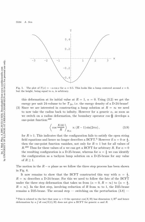
a lump centered at x = 0 (see Fig. 5). At this stage however the amplitude α is
arbitrary, and hence the lump has arbitrary height. Since the boundary pertur-
bation (3.8) is marginal, the energy of the configuration stays constant during
gIn our convention left and right refers to the antiholomorphic and holomorphic components ofthe field respectively.
Int.
J. M
od. P
hys.
A 2
005.
20:5
513-
5656
. Dow
nloa
ded
from
ww
w.w
orld
scie
ntif
ic.c
omby
UN
IVE
RSI
TY
OF
ILL
INO
IS A
T U
RB
AN
A C
HA
MPA
IGN
on
05/1
4/13
. For
per
sona
l use
onl
y.
September 29, 2005 17:21 WSPC/139-IJMPA 02519
5534 A. Sen
-3 -2 -1 1 2 3x
-0.4
-0.2
0.2
0.4
T
Fig. 5. The plot of T (x) = −α cos x for α = 0.5. This looks like a lump centered around x = 0,but the height, being equal to α, is arbitrary.
this deformation at its initial value at R = 1, α = 0. Using (3.2) we get the
energy per unit 24-volume to be T 24, i.e. the energy density of a D-24-brane!
(3) Since we are interested in constructing a lump solution at R = ∞ we need
to now take the radius back to infinity. However for a generic α, as soon as
we switch on a radius deformation, the boundary operator cos XR develops a
one-point function:468
⟨
cosX(0)
R
⟩
R;α
∝ (R − 1) sin(2πα) , (3.9)
for R ' 1. This indicates that the configuration fails to satisfy the open string
field equations and hence no longer describes a BCFT.h However if α = 0 or 12 ,
then the one-point function vanishes, not only for R ' 1 but for all values of
R.468 Thus for these values of α we can get a BCFT for arbitrary R. For α = 0
the resulting configuration is a D-25-brane, whereas for α = 12 we can identify
the configuration as a tachyon lump solution on a D-25-brane for any value
of R ≥ 1.
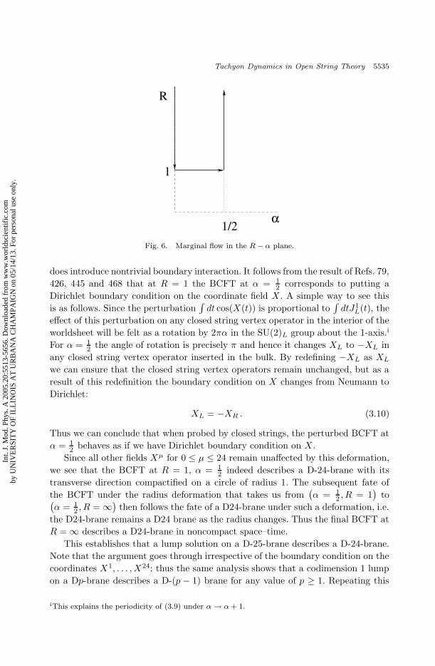
The motion in the R−α plane as we follow the three step process has been shown
in Fig. 6.
It now remains to show that the BCFT constructed this way with α = 12 ,
R = ∞ describes a D-24-brane. For this we need to follow the fate of the BCFT
under the three step deformation that takes us from (α = 0, R = ∞) to(
α = 12 ,
R = ∞)
. In the first step, involving reduction of R from ∞ to 1, the D25-brane
remains a D25-brane. The second step — switching on the perturbation (3.8) —
hThis is related to the fact that near α = 0 the operator cos(X/R) has dimension 1/R2 and hencedeformation by α
∫
dt cos(X(t)/R) does not give a BCFT for generic α and R.
Int.
J. M
od. P
hys.
A 2
005.
20:5
513-
5656
. Dow
nloa
ded
from
ww
w.w
orld
scie
ntif
ic.c
omby
UN
IVE
RSI
TY
OF
ILL
INO
IS A
T U
RB
AN
A C
HA
MPA
IGN
on
05/1
4/13
. For
per
sona
l use
onl
y.
September 29, 2005 17:21 WSPC/139-IJMPA 02519
Tachyon Dynamics in Open String Theory 5535
R
1/2
1
α
Fig. 6. Marginal flow in the R − α plane.
does introduce nontrivial boundary interaction. It follows from the result of Refs. 79,
426, 445 and 468 that at R = 1 the BCFT at α = 12 corresponds to putting a
Dirichlet boundary condition on the coordinate field X . A simple way to see this
is as follows. Since the perturbation∫
dt cos(X(t)) is proportional to∫
dtJ1L(t), the
effect of this perturbation on any closed string vertex operator in the interior of the
worldsheet will be felt as a rotation by 2πα in the SU(2)L group about the 1-axis.i
For α = 12 the angle of rotation is precisely π and hence it changes XL to −XL in
any closed string vertex operator inserted in the bulk. By redefining −XL as XL
we can ensure that the closed string vertex operators remain unchanged, but as a
result of this redefinition the boundary condition on X changes from Neumann to
Dirichlet:
XL = −XR . (3.10)
Thus we can conclude that when probed by closed strings, the perturbed BCFT at
α = 12 behaves as if we have Dirichlet boundary condition on X .
Since all other fields Xµ for 0 ≤ µ ≤ 24 remain unaffected by this deformation,
we see that the BCFT at R = 1, α = 12 indeed describes a D-24-brane with its
transverse direction compactified on a circle of radius 1. The subsequent fate of
the BCFT under the radius deformation that takes us from(
α = 12 , R = 1
)
to(
α = 12 , R = ∞
)
then follows the fate of a D24-brane under such a deformation, i.e.
the D24-brane remains a D24 brane as the radius changes. Thus the final BCFT at
R = ∞ describes a D24-brane in noncompact space–time.
This establishes that a lump solution on a D-25-brane describes a D-24-brane.
Note that the argument goes through irrespective of the boundary condition on the
coordinates X1, . . . , X24; thus the same analysis shows that a codimension 1 lump
on a Dp-brane describes a D-(p − 1) brane for any value of p ≥ 1. Repeating this
iThis explains the periodicity of (3.9) under α → α + 1.
Int.
J. M
od. P
hys.
A 2
005.
20:5
513-
5656
. Dow
nloa
ded
from
ww
w.w
orld
scie
ntif
ic.c
omby
UN
IVE
RSI
TY
OF
ILL
INO
IS A
T U
RB
AN
A C
HA
MPA
IGN
on
05/1
4/13
. For
per
sona
l use
onl
y.
September 29, 2005 17:21 WSPC/139-IJMPA 02519
5536 A. Sen
procedure q-times we can also establish that a codimension q lump on a Dp-brane
describes a D-(p− q)-brane.
This establishes the third conjecture of Subsec. 2.3. This in turn indirectly proves
Conjectures 1 and 2 as well. To see how Conjecture 1 follows from Conjecture 3,
we note that D24-brane, and hence the lump solution, has a finite energy per unit
24-volume. This means that the lump solution must have vanishing energy density
as x25 → ±∞, since otherwise we would get infinite energy per unit 24-volume by
integrating the energy density in the x25 direction. Thus if T0 denotes the value to
which T approaches as x25 → ±∞, then the total energy density must vanish at
T = T0. Furthermore T0 must be a local extremum of the potential in order for the
tachyon equation of motion to be satisfied as x25 → ±∞. This shows the existence
of a local extremum of the potential where the total energy density vanishes, as
stated in Conjecture 1.
To see how the second conjecture arises, note that D24-brane and hence the lump
solution supports open strings with ends moving on the x25 = 0 plane. This means
that if we go far away from the lump solution in the x25 direction, then there are no
physical open string excitations in this region. Since the tachyon field configuration
in this region is by definition the T = T0 configuration, we arrive at the second
conjecture that around T = T0 there are no physical open string excitations.
Finally we note that our analysis leading to the BCFT associated with the
tachyon lump solution is somewhat indirect. One could ask if in the diagram shown
in Fig. 6 it is possible to go from α = 0 to α = 12 at any value of R > 1 directly,
without following the circuitous route of first going down to R = 1 and coming
back to the desired value of R after switching on the α-deformation. It turn out
that it is possible to do this, but not via marginal deformation. For a generic value
of R, we need to perturb the BCFT describing D25-brane by an operator
−α∫
dt cos(X(t)/R) , (3.11)
which has dimension R−2 and hence is a relevant operator for R > 1. It is known
that under this relevant perturbation the original BCFT describing the D25-brane
flows into another BCFT corresponding to putting Dirichlet boundary condition
on X coordinate.146,222 In other words, although for a generic α the perturbation
(3.11) breaks conformal invariance, for a specific value of α corresponding to the
infrared fixed point, (3.11) describes a new BCFT describing the D-24-brane. j By
the usual correspondence between equations of motion in string theory and two-
dimensional BCFT, we would then conclude that open string field theory on a D-
25-brane compactified on a circle of radius R > 1 has a classical solution describing
a D24-brane. This classical solution can be identified as the lump.
jOf course this will, as usual, also induce flow in various other coupling constants labeling theboundary interactions. The precise description of these flows will depend on the renormalizationscheme, and we could choose a suitable renormalization scheme where the other coupling constantsdo not flow. In space–time language, this amounts to integrating out the other fields.
Int.
J. M
od. P
hys.
A 2
005.
20:5
513-
5656
. Dow
nloa
ded
from
ww
w.w
orld
scie
ntif
ic.c
omby
UN
IVE
RSI
TY
OF
ILL
INO
IS A
T U
RB
AN
A C
HA
MPA
IGN
on
05/1
4/13
. For
per
sona
l use
onl
y.
September 29, 2005 17:21 WSPC/139-IJMPA 02519
Tachyon Dynamics in Open String Theory 5537
The operator − cos(
XR
)
looks ill defined in the R → ∞ limit, but the correct
procedure is to expand this in powers of XR and keep the leading term. This amounts
to perturbing the D25-brane BCFT by an operator proportional to∫
dtX(t)2 . (3.12)
In the infrared this perturbation takes us to the BCFT of a D24-brane, localized
at x = 0. This result is useful in the study of tachyon condensation in boundary
string field theory,180,317,318 and will be made use of in Sec. 5.
3.2. Superstring theory
In this section we shall generalize the analysis of Subsec. 3.1 to superstring theory
showing that various classical solutions involving the tachyon on D9–D9-brane pair
of IIB or non-BPS D9-brane of IIA represent lower dimensional Dp-branes. For
definiteness we shall illustrate in detail the representation of a non-BPS D8-brane
of IIB as a kink solution on a D9–D9-brane pair465 (case 3(b) in Subsec. 2.1), and
then briefly comment on the other cases.
The tachyon state on a D9–D9-brane system comes from open strings with one
leg on the D9-brane and the other leg on the D9-brane. Thus the corresponding
vertex operator will carry an off-diagonal Chan–Paton factor which we can take to
be the Pauli matrix σ1 or σ2. This gives rise to two real tachyon fields T1 and T2
on the worldvolume of this D-brane system, which can be combined into a complex
tachyon T = T1+iT2. Thus in this convention the coefficients of σ1 and σ2 represent
the real and imaginary parts respectively of the complex tachyon field. We shall
show that a tachyonic kink involving the real part T1 of T , with the imaginary part
set to zero, represents a non-BPS D8-brane.
The vertex operator of the tachyon T1 carrying momentum k in the −1
picture157,158 is given byk
V−1(k) = ce−φgeik·X ⊗ σ1 , (3.13)
where φg is the bosonic field arising out of bosonization of the β-γ ghost system.158
As usual this vertex operator is inserted at the boundary of the worldsheet. The
on-shell condition is
k2 =1
2, (3.14)
showing that the corresponding state has mass2 = − 12 . The same vertex operator
in the 0 picture is
V0 = −√
2ck · ψeik·X ⊗ σ1 , (3.15)
kA brief review of bosonization of superconformal ghosts, picture changing and physical openstring vertex operators in superstring theory is given at the beginning of Subsec. 4.6.
Int.
J. M
od. P
hys.
A 2
005.
20:5
513-
5656
. Dow
nloa
ded
from
ww
w.w
orld
scie
ntif
ic.c
omby
UN
IVE
RSI
TY
OF
ILL
INO
IS A
T U
RB
AN
A C
HA
MPA
IGN
on
05/1
4/13
. For
per
sona
l use
onl
y.
September 29, 2005 17:21 WSPC/139-IJMPA 02519
5538 A. Sen
where ψµ is boundary value of the worldsheet superpartners ψµL or ψµ
R of Xµ. On
the boundary ψµL and ψµ
R are equal. The fields φg and ψµ are normalized so that
their left- and right-moving components satisfy the operator product expansion:
∂φgR(z)∂φgR(w) ' − 1
(z − w)2, ∂φgL(z)∂φgL(w) ' − 1
(z − w)2,
ψµR(z)ψν
R(w) ' ηµν
z − w, ψµ
L(z)ψνL(w) ' ηµν
z − w.
(3.16)
In order to show that the kink solution involving this tachyon represents a non-
BPS D8-brane, we proceed exactly as in the case of bosonic string theory, i.e. we
first find the BCFT associated with the tachyonic kink solution on the D9–D9-brane
pair, and then show that this BCFT is identical to that of a non-BPS D8-brane.
In order to find the BCFT associated with the tachyonic kink, we need to identify
a series of steps which take us from the T = 0 configuration to the tachyonic kink
configuration. This is done as follows:465
(1) We first compactify the x ≡ x9 direction into a circle of radius R. We would
like to take the radius to an appropriate critical value (analog of R = 1 in the
bosonic case) where we can create a kink solution via a marginal boundary
deformation. However, in order to create a single kink on a circle, we need to
have a configuration where the tachyon is antiperiodic along the circle. This
can be achieved by switching on half a unit of Wilson line along the circle
associated with one of the branes, since the tachyon field is charged under this
gauge field. This is a boundary marginal deformation.
(2) In the presence of this Wilson line, a configuration of the form
T1(x) =√
2α sinx
2R, (3.17)
is an allowed configuration and has the shape of a kink solution (see Fig. 7).
Here the normalization factor of√
2 has been chosen for convenience. The
corresponding vertex operators in the −1 and the 0 pictures are given by,
respectively,
V−1 = ce−φg sinX
2R⊗ σ1 , (3.18)
and
V0 =i√2R
cψ cosX
2R⊗ σ1 , (3.19)
where X ≡ X9, ψ ≡ ψ9. Thus switching on a background tachyon of the form
(3.17) corresponds to adding a worldsheet perturbation
iα
R
∫
dt ψ cosX
2R⊗ σ1 . (3.20)
Int.
J. M
od. P
hys.
A 2
005.
20:5
513-
5656
. Dow
nloa
ded
from
ww
w.w
orld
scie
ntif
ic.c
omby
UN
IVE
RSI
TY
OF
ILL
INO
IS A
T U
RB
AN
A C
HA
MPA
IGN
on
05/1
4/13
. For
per
sona
l use
onl
y.
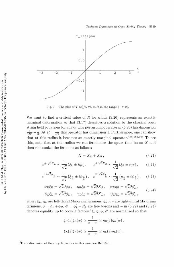
September 29, 2005 17:21 WSPC/139-IJMPA 02519
Tachyon Dynamics in Open String Theory 5539
-3 -2 -1 1 2 3x-R
-1
-0.5
0.5
1
T_1/alpha
Fig. 7. The plot of T1(x)/α vs. x/R in the range (−π, π).
We want to find a critical value of R for which (3.20) represents an exactly
marginal deformation so that (3.17) describes a solution to the classical open
string field equations for any α. The perturbing operator in (3.20) has dimension1
4R2 + 12 . At R = 1√
2this operator has dimension 1. Furthermore, one can show
that at this radius it becomes an exactly marginal operator.465,164,165 To see
this, note that at this radius we can fermionize the space–time boson X and
then rebosonize the fermions as follows:
X = XL +XR , (3.21)
e±i√
2XL ∼ 1√2
(ξL ± iηL) , e±i√
2XR ∼ 1√2
(ξR ± iηR) , (3.22)
e±i
√2φ L
R ∼ 1√2
(
ξ LR± iψ L
R
)
, e±i
√2φ′
LR ∼ 1√
2
(
η LR± iψ L
R
)
, (3.23)
ψRξR =√
2∂φR , ηRξR =√
2∂XR , ψRηR =√
2∂φ′R ,
ψLξL =√
2∂φL , ηLξL =√
2∂XL , ψLηL =√
2∂φ′L ,(3.24)
where ξL, ηL are left-chiral Majorana fermions, ξR, ηR are right-chiral Majorana
fermions, φ = φL +φR, φ′ = φ′L +φ′R are free bosons and ∼ in (3.22) and (3.23)
denotes equality up to cocycle factors.l ξ, η, φ, φ′ are normalized so that
ξR(z)ξR(w) ' 1
z − w' ηR(z)ηR(w) ,
ξL(z)ξL(w) ' 1
z − w' ηL(z)ηL(w) ,
lFor a discussion of the cocycle factors in this case, see Ref. 346.
Int.
J. M
od. P
hys.
A 2
005.
20:5
513-
5656
. Dow
nloa
ded
from
ww
w.w
orld
scie
ntif
ic.c
omby
UN
IVE
RSI
TY
OF
ILL
INO
IS A
T U
RB
AN
A C
HA
MPA
IGN
on
05/1
4/13
. For
per
sona
l use
onl
y.
September 29, 2005 17:21 WSPC/139-IJMPA 02519
5540 A. Sen
∂φR(z)∂φR(w) ' − 1
2(z − w)2,
∂φL(z)∂φL(w) ' − 1
2(z − w)2,
∂φ′R(z)∂φ′R(w) ' − 1
2(z − w)2,
∂φ′L(z)∂φ′L(w) ' − 1
2(z − w)2. (3.25)
Equation (3.22) defines ξL,R and ηL,R in terms of XL,R, and Eq. (3.23) defines
φL,R and φ′L,R in terms of ξL,R, ηL,R and ψL,R. Equation (3.24) follows from
(3.22), (3.23) and the usual rules for bosonization. The boundary conditions on
various fields, following from Neumann boundary condition on X and ψ, and
Eqs. (3.22)–(3.24), are
XL = XR , ψL = ψR , ξL = ξR ,
ηL = ηR , φL = φR , φ′L = φ′R .(3.26)
Using Eqs. (3.21)–(3.26) the boundary perturbation (3.20) takes the form
i√
2α
∫
dt ∂φL(t) ⊗ σ1 . (3.27)
This corresponds to switching on a Wilson line along the φ direction and is
clearly an exactly marginal deformation. Thus for any value of the coefficient
α in (3.27) (and hence in (3.20)) we get a boundary CFT.
(3) In order to create a kink solution in the noncompact theory, we need to take the
radius R back to infinity after switching on the deformation (3.20). However
here we encounter an obstruction; for generic α the boundary vertex operator
(3.20) develops a one-point function on the upper half plane465 for R 6= 1√2:
⟨
ψ cosX
2R(0) ⊗ σ1
⟩
UHP
∝ (R − 1) sin(2πα) . (3.28)
This is a reflection of the fact that for R 6= 1√2
the operator ψ cos(X/2R) is no
longer marginal. This shows that in order to take the radius back to ∞, α must
be fixed at 0 or 12 . α = 0 gives us back the original D-brane system, whereas
α = 12 gives the kink solution.
To summarize, in order to construct the tachyon kink solution on a D9–D9 brane
pair we first compactify the x direction on a circle of radius 1√2
and switch on half
unit of Wilson line along x on one of the branes, then switch on the deformation
(3.20) and take α to 12 , and finally takeR back to infinity. This gives the construction
of the tachyonic kink configuration on a D9–D9-brane pair as a BCFT. It now
remains to show that this BCFT actually describes a non-BPS D8-brane, i.e. the
effect of this deformation is to change the Neumann boundary condition on X
Int.
J. M
od. P
hys.
A 2
005.
20:5
513-
5656
. Dow
nloa
ded
from
ww
w.w
orld
scie
ntif
ic.c
omby
UN
IVE
RSI
TY
OF
ILL
INO
IS A
T U
RB
AN
A C
HA
MPA
IGN
on
05/1
4/13
. For
per
sona
l use
onl
y.
September 29, 2005 17:21 WSPC/139-IJMPA 02519
Tachyon Dynamics in Open String Theory 5541
and ψL, ψR to Dirichlet boundary condition. This is done by noting that (3.27)
is the contour integral of an antiholomorphic current, and hence the effect of this
on a correlation function can be studied by deforming the contour and picking up
residues from various operators. Using Eqs. (3.21)–(3.23) it is easy to see that for
α = 12 , the exponential of (3.27) transforms the left-moving fermions ξL, ηL and
ψL as
ξL → −ξL , ηL → ηL , ψL → −ψL . (3.29)
In terms of the original fields, this induces a transformation ∂XL → −∂XL, ψL →−ψL on every vertex operator inserted in the interior of the worldsheet. The right-
moving worldsheet fields are not affected. By a redefinition XL → −XL, ψL →−ψL, we can leave the vertex operators unchanged, but this changes the boundary
condition on X and ψ from Neumann to Dirichlet:
∂XL = −∂XR , ψL = −ψR . (3.30)
This clearly shows that switching on the deformation (3.27) with α = 12 corresponds
to creating a D8-brane transverse to the circle of radius R = 1√2. Taking the radius
back to infinity leaves the D8-brane unchanged.
The analysis can be generalized in many different ways. First of all, since the
boundary condition on X0, . . . , X8 played no role in the analysis, we can choose
them to be anything that we like. This establishes in general that a kink solution on
a Dp–Dp-brane pair represents a non-BPS D-(p − 1)-brane. The analysis showing
that a kink solution on a non-BPS D-p-brane represents a BPS D-(p − 1)-brane
is essentially identical. We begin with the kink solution on the BPS Dp–Dp-brane
pair in type IIB/IIA theory for p odd/even and mod this out by (−1)FL . This
converts type IIB/IIA theory to type IIA/IIB theory, the Dp–Dp-brane pair to a
non-BPS D-p-brane, and the non-BPS D-(p− 1)-brane to a BPS D-(p− 1)-brane.m
This shows that the kink solution on a non-BPS D-p-brane can be identified as a
BPS D-(p− 1)-brane. Finally the analysis showing that a codimension k soliton on
a Dp–Dp-brane pair or a non-BPS Dp brane produces a D-(p − k)-brane can be
done by compactifying k of the coordinates tangential to the original D-brane on
a torus T k of appropriate radii, switching on a marginal deformation that creates
the codimension k soliton, and finally proving that the BCFT obtained at the end
of this marginal deformation is a D-(p− k)-brane.346
3.3. Analysis of the boundary state
Given a boundary CFT describing a D-brane system, we can associate with it a
boundary state |B〉.1,78,205,126,127 This is a closed string state of ghost number 3,
and has the following property. Given any closed string state |V 〉 and the associated
mOne can show541,467 that the tachyon state as well as all other open string states on a non-BPSD-brane carrying Chan–Paton factor σ1 are odd under (−1)FL . Thus these modes are projectedout after modding out the theory by (−1)FL , and we get a tachyon free BPS D-brane.
Int.
J. M
od. P
hys.
A 2
005.
20:5
513-
5656
. Dow
nloa
ded
from
ww
w.w
orld
scie
ntif
ic.c
omby
UN
IVE
RSI
TY
OF
ILL
INO
IS A
T U
RB
AN
A C
HA
MPA
IGN
on
05/1
4/13
. For
per
sona
l use
onl
y.
September 29, 2005 17:21 WSPC/139-IJMPA 02519
5542 A. Sen
vertex operator V , the BPZ inner product 〈B|V 〉 is given by the one-point function
of V inserted at the centre of a unit disk D, the boundary condition on ∂D being
the one associated with the particular boundary CFT under consideration:
〈B|V 〉 ∝ 〈V (0)〉D . (3.31)
Note that in order to find the contribution to the boundary state at oscillator level
(N,N), we only need to compute the inner product of the boundary state with
closed string states of level (N,N). This in turn requires computation of one-point
function on the disk of closed string vertex operators of level (N,N).
From the definition (3.31) it is clear that the boundary state contains infor-
mation about what kind of source for the closed string states is produced by the
D-brane system under consideration. This has been made more precise in App. A.
There it has been shown that if the boundary state |B〉 associated with a D-brane
in bosonic string theory has an expansion of the form
|B〉 =
∫
d26k
(2π)26[F (k) + (Aµν(k) + Cµν(k))αµ
−1αν−1
+ B(k)(b−1c−1 + b−1c−1) + · · ·](c0 + c0)c1c1|k〉 , (3.32)
where F , Aµν = Aνµ, Cµν = −Cνµ, B, etc. are fixed functions, αµ−n, αµ
−n are
oscillators of Xµ, and b−n, c−n, b−n, c−n are ghost oscillators, then the energy–
momentum tensor Tµν(x), defined as the source for the graviton field, is given by
Tµν(x) ∝ (Aµν(x) + ηµνB(x)) . (3.33)
We shall choose the normalization of |B〉 in such a way that the above equation
takes the form
Tµν(x) =1
2(Aµν(x) + ηµνB(x)) . (3.34)
Let us apply this to the specific D-brane system studied in Subsec. 3.1, namely
D-p-brane wrapped on a circle of radius 1. We take the directions transverse to
the brane to be x1, . . . , x25−p, and the spatial directions along the brane to be
x26−p, . . . , x25. The boundary state of the initial D-p-brane without any perturba-
tion is given by1,78,205,126,127
|B〉 = T p|B〉c=1 ⊗ |B〉c=25 ⊗ |B〉ghost , (3.35)
where T p is the tension of the Dp-brane as given in (2.20), |B〉c=1 denotes the
boundary state associated with the X25 ≡ X direction, |B〉c=25 denotes the bound-
ary state associated with the other 25 directions X0, . . . , X24, and |B〉ghost denotes
the boundary state associated with the ghost direction. We have
|B〉c=25 =
∫
d25−pk⊥(2π)25−p
exp
(
25∑
µ,ν=0
∞∑
n=1
1
nηµν(−1)dµαµ
−nαν−n
)
|k‖ = 0, k⊥〉 , (3.36)
|B〉ghost = exp
(
−∞∑
n=1
(b−nc−n + b−nc−n)
)
(c0 + c0)c1c1|0〉 , (3.37)
Int.
J. M
od. P
hys.
A 2
005.
20:5
513-
5656
. Dow
nloa
ded
from
ww
w.w
orld
scie
ntif
ic.c
omby
UN
IVE
RSI
TY
OF
ILL
INO
IS A
T U
RB
AN
A C
HA
MPA
IGN
on
05/1
4/13
. For
per
sona
l use
onl
y.
September 29, 2005 17:21 WSPC/139-IJMPA 02519
Tachyon Dynamics in Open String Theory 5543
and
|B〉c=1 =
∞∑
m=−∞exp
(
−∞∑
n=1
1
nα−nα−n
)
|k = 0, w = m〉 , (3.38)
where dµ = 1 for Neumann directions and 0 for Dirichlet directions, k‖ denotes
momentum along the D-p-brane in directions other than x25, k⊥ denotes momentum
transverse to the D-p-brane, αn, αn without any superscript denote the X25 ≡ X
oscillators, and k and w denote the momentum and winding number respectively
along the circle along x25. Let us denote by xM the coordinates other than x25 ≡ x
along the D-p-brane worldvolume, and by xm the coordinates transverse to the D-p-
brane worldvolume. We shall choose M to run over the values 0 and (26−p), . . . , 24
and m to run over the values 1, . . . , (25 − p). Expanding the boundary state in
powers of the various oscillators, and comparing this expansion with (3.32), we get
the following nonzero components of Aµν and B:
Axx = −T pδ(x⊥) , AMN = −T pηMNδ(x⊥) ,
Amn = T pδmnδ(x⊥) , B = −T pδ(x⊥) ,(3.39)
and hence
Txx = −T pδ(x⊥) , TMN = −T pηMNδ(x⊥) , Tmn = 0 . (3.40)
This is the energy–momentum tensor associated with a D-25-brane.
We shall now study the change in the boundary state under the deformation
of the boundary CFT by the marginal operator (3.8).79,445 Using the boundary
condition (3.6) we can rewrite (3.8) as
−α∫
dt cos(2XL(t))dt = −α∫
dt J1L(t) . (3.41)
Adding such a perturbation at the boundary effectively rotates the left-moving
worldsheet component of the boundary state by an angle 2πα about the 1-axis. In
particular for α = 12 , the effect of this perturbation is a rotation by π about the
1-axis which changes J3L to −J3
L, i.e. αn to −αn in the exponent of (3.38), and also
converts the winding number w = m to momentum k = m along x25. Thus |B〉c=1
is transformed to
∞∑
m=−∞exp
( ∞∑
n=1
1
nα−nα−n
)
|k = m,w = 0〉 . (3.42)
The other components of |B〉 given in (3.36), (3.37) remain unchanged. The result
is precisely the boundary state associated with a D-(p − 1)-brane, and the corre-
sponding Tµν computed using (3.32) and (3.34) precisely reproduces the energy–
momentum tensor of a D-(p − 1)-brane situated at x = 0. We shall shortly derive
this as a special case of a more general result.
Int.
J. M
od. P
hys.
A 2
005.
20:5
513-
5656
. Dow
nloa
ded
from
ww
w.w
orld
scie
ntif
ic.c
omby
UN
IVE
RSI
TY
OF
ILL
INO
IS A
T U
RB
AN
A C
HA
MPA
IGN
on
05/1
4/13
. For
per
sona
l use
onl
y.
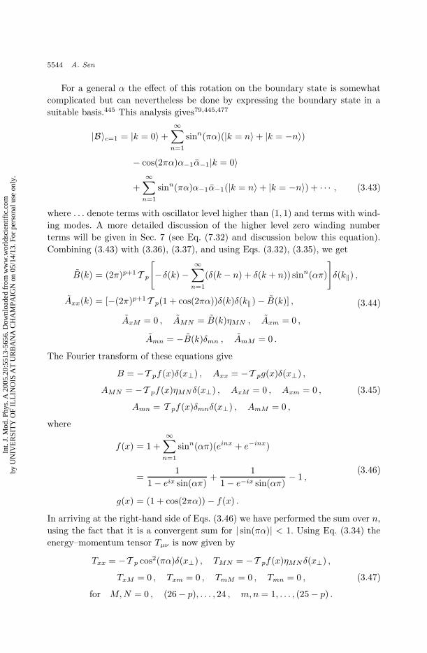
September 29, 2005 17:21 WSPC/139-IJMPA 02519
5544 A. Sen
For a general α the effect of this rotation on the boundary state is somewhat
complicated but can nevertheless be done by expressing the boundary state in a
suitable basis.445 This analysis gives79,445,477
|B〉c=1 = |k = 0〉 +
∞∑
n=1
sinn(πα)(|k = n〉 + |k = −n〉)
− cos(2πα)α−1α−1|k = 0〉
+∞∑
n=1
sinn(πα)α−1α−1(|k = n〉 + |k = −n〉) + · · · , (3.43)
where . . . denote terms with oscillator level higher than (1, 1) and terms with wind-
ing modes. A more detailed discussion of the higher level zero winding number
terms will be given in Sec. 7 (see Eq. (7.32) and discussion below this equation).
Combining (3.43) with (3.36), (3.37), and using Eqs. (3.32), (3.35), we get
B(k) = (2π)p+1T p
[
−δ(k) −∞∑
n=1
(δ(k − n) + δ(k + n)) sinn(απ)
]
δ(k‖) ,
Axx(k) = [−(2π)p+1T p(1 + cos(2πα))δ(k)δ(k‖) − B(k)] ,
AxM = 0 , AMN = B(k)ηMN , Axm = 0 ,
Amn = −B(k)δmn , AmM = 0 .
(3.44)
The Fourier transform of these equations give
B = −T pf(x)δ(x⊥) , Axx = −T pg(x)δ(x⊥) ,
AMN = −T pf(x)ηMNδ(x⊥) , AxM = 0 , Axm = 0 ,
Amn = T pf(x)δmnδ(x⊥) , AmM = 0 ,
(3.45)
where
f(x) = 1 +
∞∑
n=1
sinn(απ)(einx + e−inx)
=1
1 − eix sin(απ)+
1
1 − e−ix sin(απ)− 1 ,
g(x) = (1 + cos(2πα)) − f(x) .
(3.46)
In arriving at the right-hand side of Eqs. (3.46) we have performed the sum over n,
using the fact that it is a convergent sum for | sin(πα)| < 1. Using Eq. (3.34) the
energy–momentum tensor Tµν is now given by
Txx = −T p cos2(πα)δ(x⊥) , TMN = −T pf(x)ηMNδ(x⊥) ,
TxM = 0 , Txm = 0 , TmM = 0 , Tmn = 0 ,
for M,N = 0 , (26− p), . . . , 24 , m, n = 1, . . . , (25 − p) .
(3.47)
Int.
J. M
od. P
hys.
A 2
005.
20:5
513-
5656
. Dow
nloa
ded
from
ww
w.w
orld
scie
ntif
ic.c
omby
UN
IVE
RSI
TY
OF
ILL
INO
IS A
T U
RB
AN
A C
HA
MPA
IGN
on
05/1
4/13
. For
per
sona
l use
onl
y.
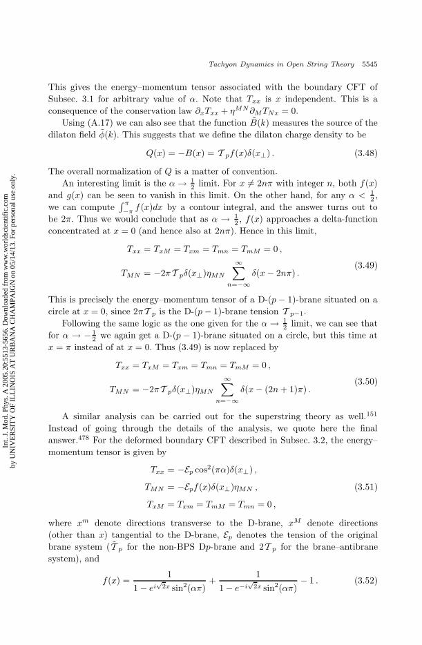
September 29, 2005 17:21 WSPC/139-IJMPA 02519
Tachyon Dynamics in Open String Theory 5545
This gives the energy–momentum tensor associated with the boundary CFT of
Subsec. 3.1 for arbitrary value of α. Note that Txx is x independent. This is a
consequence of the conservation law ∂xTxx + ηMN∂MTNx = 0.
Using (A.17) we can also see that the function B(k) measures the source of the
dilaton field φ(k). This suggests that we define the dilaton charge density to be
Q(x) = −B(x) = T pf(x)δ(x⊥) . (3.48)
The overall normalization of Q is a matter of convention.
An interesting limit is the α → 12 limit. For x 6= 2nπ with integer n, both f(x)
and g(x) can be seen to vanish in this limit. On the other hand, for any α < 12 ,
we can compute∫ π
−πf(x)dx by a contour integral, and the answer turns out to
be 2π. Thus we would conclude that as α → 12 , f(x) approaches a delta-function
concentrated at x = 0 (and hence also at 2nπ). Hence in this limit,
Txx = TxM = Txm = Tmn = TmM = 0 ,
TMN = −2πT pδ(x⊥)ηMN
∞∑
n=−∞δ(x− 2nπ) .
(3.49)
This is precisely the energy–momentum tensor of a D-(p − 1)-brane situated on a
circle at x = 0, since 2πT p is the D-(p− 1)-brane tension T p−1.
Following the same logic as the one given for the α → 12 limit, we can see that
for α → − 12 we again get a D-(p − 1)-brane situated on a circle, but this time at
x = π instead of at x = 0. Thus (3.49) is now replaced by
Txx = TxM = Txm = Tmn = TmM = 0 ,
TMN = −2πT pδ(x⊥)ηMN
∞∑
n=−∞δ(x− (2n+ 1)π) .
(3.50)
A similar analysis can be carried out for the superstring theory as well.151
Instead of going through the details of the analysis, we quote here the final
answer.478 For the deformed boundary CFT described in Subsec. 3.2, the energy–
momentum tensor is given by
Txx = −Ep cos2(πα)δ(x⊥) ,
TMN = −Epf(x)δ(x⊥)ηMN ,
TxM = Txm = TmM = Tmn = 0 ,
(3.51)
where xm denote directions transverse to the D-brane, xM denote directions
(other than x) tangential to the D-brane, Ep denotes the tension of the original
brane system ( T p for the non-BPS Dp-brane and 2T p for the brane–antibrane
system), and
f(x) =1
1 − ei√
2x sin2(απ)+
1
1− e−i√
2x sin2(απ)− 1 . (3.52)
Int.
J. M
od. P
hys.
A 2
005.
20:5
513-
5656
. Dow
nloa
ded
from
ww
w.w
orld
scie
ntif
ic.c
omby
UN
IVE
RSI
TY
OF
ILL
INO
IS A
T U
RB
AN
A C
HA
MPA
IGN
on
05/1
4/13
. For
per
sona
l use
onl
y.
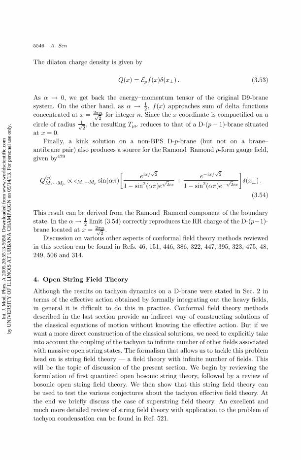
September 29, 2005 17:21 WSPC/139-IJMPA 02519
5546 A. Sen
The dilaton charge density is given by
Q(x) = Epf(x)δ(x⊥) . (3.53)
As α → 0, we get back the energy–momentum tensor of the original D9-brane
system. On the other hand, as α → 12 , f(x) approaches sum of delta functions
concentrated at x = 2πn√2
for integer n. Since the x coordinate is compactified on a
circle of radius 1√2, the resulting Tµν reduces to that of a D-(p− 1)-brane situated
at x = 0.
Finally, a kink solution on a non-BPS D-p-brane (but not on a brane–
antibrane pair) also produces a source for the Ramond–Ramond p-form gauge field,
given by479
Q(p)M1···Mp
∝ εM1···Mpsin(απ)
[
eix/√
2
1 − sin2(απ)e√
2ix+
e−ix/√
2
1 − sin2(απ)e−√
2ix
]
δ(x⊥) .
(3.54)
This result can be derived from the Ramond–Ramond component of the boundary
state. In the α → 12 limit (3.54) correctly reproduces the RR charge of the D-(p−1)-
brane located at x = 2πn√2
.
Discussion on various other aspects of conformal field theory methods reviewed
in this section can be found in Refs. 46, 151, 446, 386, 322, 447, 395, 323, 475, 48,
249, 506 and 314.
4. Open String Field Theory
Although the results on tachyon dynamics on a D-brane were stated in Sec. 2 in
terms of the effective action obtained by formally integrating out the heavy fields,
in general it is difficult to do this in practice. Conformal field theory methods
described in the last section provide an indirect way of constructing solutions of
the classical equations of motion without knowing the effective action. But if we
want a more direct construction of the classical solutions, we need to explicitly take
into account the coupling of the tachyon to infinite number of other fields associated
with massive open string states. The formalism that allows us to tackle this problem
head on is string field theory — a field theory with infinite number of fields. This
will be the topic of discussion of the present section. We begin by reviewing the
formulation of first quantized open bosonic string theory, followed by a review of
bosonic open string field theory. We then show that this string field theory can
be used to test the various conjectures about the tachyon effective field theory. At
the end we briefly discuss the case of superstring field theory. An excellent and
much more detailed review of string field theory with application to the problem of
tachyon condensation can be found in Ref. 521.
Int.
J. M
od. P
hys.
A 2
005.
20:5
513-
5656
. Dow
nloa
ded
from
ww
w.w
orld
scie
ntif
ic.c
omby
UN
IVE
RSI
TY
OF
ILL
INO
IS A
T U
RB
AN
A C
HA
MPA
IGN
on
05/1
4/13
. For
per
sona
l use
onl
y.
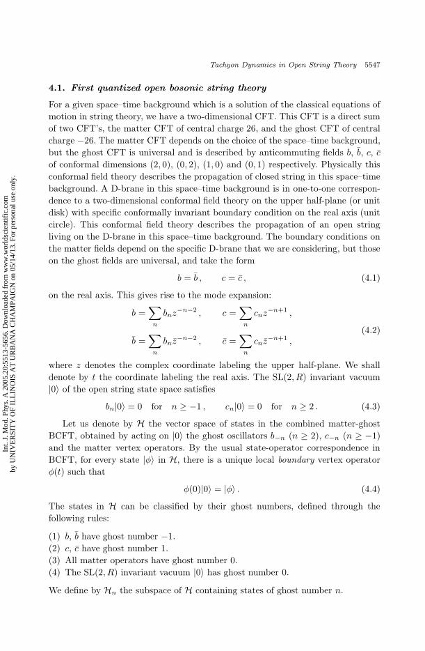
September 29, 2005 17:21 WSPC/139-IJMPA 02519
Tachyon Dynamics in Open String Theory 5547
4.1. First quantized open bosonic string theory
For a given space–time background which is a solution of the classical equations of
motion in string theory, we have a two-dimensional CFT. This CFT is a direct sum
of two CFT’s, the matter CFT of central charge 26, and the ghost CFT of central
charge −26. The matter CFT depends on the choice of the space–time background,
but the ghost CFT is universal and is described by anticommuting fields b, b, c, c
of conformal dimensions (2, 0), (0, 2), (1, 0) and (0, 1) respectively. Physically this
conformal field theory describes the propagation of closed string in this space–time
background. A D-brane in this space–time background is in one-to-one correspon-
dence to a two-dimensional conformal field theory on the upper half-plane (or unit
disk) with specific conformally invariant boundary condition on the real axis (unit
circle). This conformal field theory describes the propagation of an open string
living on the D-brane in this space–time background. The boundary conditions on
the matter fields depend on the specific D-brane that we are considering, but those
on the ghost fields are universal, and take the form
b = b , c = c , (4.1)
on the real axis. This gives rise to the mode expansion:
b =∑
n
bnz−n−2 , c =
∑
n
cnz−n+1 ,
b =∑
n
bnz−n−2 , c =
∑
n
cnz−n+1 ,
(4.2)
where z denotes the complex coordinate labeling the upper half-plane. We shall
denote by t the coordinate labeling the real axis. The SL(2, R) invariant vacuum
|0〉 of the open string state space satisfies
bn|0〉 = 0 for n ≥ −1 , cn|0〉 = 0 for n ≥ 2 . (4.3)
Let us denote by H the vector space of states in the combined matter-ghost
BCFT, obtained by acting on |0〉 the ghost oscillators b−n (n ≥ 2), c−n (n ≥ −1)
and the matter vertex operators. By the usual state-operator correspondence in
BCFT, for every state |φ〉 in H, there is a unique local boundary vertex operator
φ(t) such that
φ(0)|0〉 = |φ〉 . (4.4)
The states in H can be classified by their ghost numbers, defined through the
following rules:
(1) b, b have ghost number −1.
(2) c, c have ghost number 1.
(3) All matter operators have ghost number 0.
(4) The SL(2, R) invariant vacuum |0〉 has ghost number 0.
We define by Hn the subspace of H containing states of ghost number n.
Int.
J. M
od. P
hys.
A 2
005.
20:5
513-
5656
. Dow
nloa
ded
from
ww
w.w
orld
scie
ntif
ic.c
omby
UN
IVE
RSI
TY
OF
ILL
INO
IS A
T U
RB
AN
A C
HA
MPA
IGN
on
05/1
4/13
. For
per
sona
l use
onl
y.
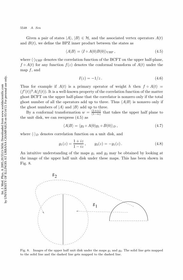
September 29, 2005 17:21 WSPC/139-IJMPA 02519
5548 A. Sen
Given a pair of states |A〉, |B〉 ∈ H, and the associated vertex operators A(t)
and B(t), we define the BPZ inner product between the states as
〈A|B〉 = 〈I A(0)B(0)〉UHP , (4.5)
where 〈·〉UHP denotes the correlation function of the BCFT on the upper half-plane,
f A(t) for any function f(z) denotes the conformal transform of A(t) under the
map f , and
I(z) = −1/z . (4.6)
Thus for example if A(t) is a primary operator of weight h then f A(t) =
(f ′(t))hA(f(t)). It is a well-known property of the correlation function of the matter
ghost BCFT on the upper half-plane that the correlator is nonzero only if the total
ghost number of all the operators add up to three. Thus 〈A|B〉 is nonzero only if
the ghost numbers of |A〉 and |B〉 add up to three.
By a conformal transformation w = (1+iz)(1−iz) that takes the upper half plane to
the unit disk, we can reexpress (4.5) as
〈A|B〉 = 〈g2 A(0)g1 B(0)〉D , (4.7)
where 〈·〉D denotes correlation function on a unit disk, and
g1(z) =1 + iz
1 − iz, g2(z) = −g1(z) . (4.8)
An intuitive understanding of the maps g1 and g2 may be obtained by looking at
the image of the upper half unit disk under these maps. This has been shown in
Fig. 8.
g1
g2
Fig. 8. Images of the upper half unit disk under the maps g1 and g2. The solid line gets mappedto the solid line and the dashed line gets mapped to the dashed line.
Int.
J. M
od. P
hys.
A 2
005.
20:5
513-
5656
. Dow
nloa
ded
from
ww
w.w
orld
scie
ntif
ic.c
omby
UN
IVE
RSI
TY
OF
ILL
INO
IS A
T U
RB
AN
A C
HA
MPA
IGN
on
05/1
4/13
. For
per
sona
l use
onl
y.
September 29, 2005 17:21 WSPC/139-IJMPA 02519
Tachyon Dynamics in Open String Theory 5549
Physical open string states on the D-brane are states in H1 satisfying the fol-
lowing criteria:
(1) The state |φ〉 must be BRST invariant:
QB |φ〉 = 0 , (4.9)
where
QB =1
2πi
[ ∮
c(z)Tm(z)dz +
∮
b(z)c∂c(z)dz
]
, (4.10)
is the BRST charge carrying ghost number 1 and satisfying
(QB)2 = 0 . (4.11)
Here Tm(z) =∑
n L(m)n z−n−2 stand for the zz component of the worldsheet
stress tensor of the matter part of the BCFT describing the D-brane.∮
denotes
a contour around the origin.
(2) Two states |φ〉 and |φ′〉 are considered equivalent if they differ by a state of the
form QB |Λ〉:
|φ〉 ≡ |φ〉 +QB |Λ〉 , (4.12)
for any state |Λ〉 ∈ H0.
Thus physical states are in one-to-one correspondence with the elements of BRST
cohomology in H1.
In the first quantized formulation there is also a well-defined prescription, known
as Polyakov prescription, for computing tree and loop amplitudes involving physical
open string states as external lines.
4.2. Formulation of open bosonic string field theory
The open string field theory describing the dynamics of a D-brane is, by definition,
a field theory satisfying the following two criteria:
(1) Gauge inequivalent solutions of the linearized equations of motion are in one-
to-one correspondence with the physical states of the open string.
(2) The S-matrix computed using the Feynman rules of the string field theory
reproduces the S-matrix computed using Polyakov prescription to all orders in
the perturbation theory.
If we are interested in studying only the classical properties of string field theory, we
can relax the second constraint a bit by requiring that the S-matrix elements agree
only at the tree level. Nevertheless for the open bosonic string field theory that we
shall be describing,535 the agreement has been verified to all orders in perturbation
theory.192
Int.
J. M
od. P
hys.
A 2
005.
20:5
513-
5656
. Dow
nloa
ded
from
ww
w.w
orld
scie
ntif
ic.c
omby
UN
IVE
RSI
TY
OF
ILL
INO
IS A
T U
RB
AN
A C
HA
MPA
IGN
on
05/1
4/13
. For
per
sona
l use
onl
y.
September 29, 2005 17:21 WSPC/139-IJMPA 02519
5550 A. Sen
The first step in the construction of string field theory will be to decide what
corresponds to a general off-shell string field configuration. Usually when one goes
from the first to second quantized formulation, the wave functions/states of the first
quantized theory become the field configurations of the second quantized theory.
However, a generic off-shell field configuration in the second quantized theory does
not satisfy the physical state condition.n This condition comes as the linearized
equation of motion of the field theory. In the same spirit we should expect that a
generic off-shell string field configuration should correspond to a state in the BCFT
without the restriction of BRST invariance, and the physical state condition, i.e. the
BRST invariance of the state, should emerge as the linearized equation of motion
of the string field theory. This however still does not uniquely fix the space of string
field configurations, since we can, for example take this to be the whole of H, or H1,
or even a subspace of H1 that contains at least one representative from each BRST
cohomology class. It turns out that the simplest form of open string field theory is
obtained by taking a general off-shell string field configuration to be a state in H1,
i.e. a state |Φ〉 in H of ghost number 1.535
Since we are attempting to construct a string field theory, one might wonder in
what sense a state |Φ〉 in H1 describes a field configuration. To see this we need to
choose a basis of states |χ1,α〉 in H1. Then we can expand |Φ〉 as
|Φ〉 =∑
α
φα|χ1,α〉 . (4.13)
Specifying |Φ〉 is equivalent to specifying the coefficients φα. Thus the set of numbers
φα labels a given string field configuration. Let us for example consider the case
of a Dp-brane in (25 + 1)-dimensional Minkowski space. We define Fock vacuum
states |k〉 labeled by (p+ 1)-dimensional momentum k along the Dp-brane as
|k〉 = eik·X(0)|0〉 . (4.14)
A generic state carrying momentum k will be created by a set of oscillators acting
on the state (4.14). Thus in this case the index α in (4.13) includes the (p + 1)-
dimensional continuous momentum index kµ along the Dp-brane, and a discrete
index r which originate from various oscillators, and runs over infinite number of
values. Hence we can write
φα → φkµ,r ≡ φr(k0, . . . , kp) ,
|χ1,α〉 → |χ1,r(k)〉 ,∑
α
→∑
r
∫
dp+1k
(2π)p+1.
(4.15)
nFor example second quantization of a nonrelativistic Schrodinger problem describing a par-ticle of mass m moving under a potential V in three dimensions is described by the action∫
dt∫
d3x Ψ∗
(
i ∂Ψ∂t
+ ~2
2m~∇2Ψ − V Ψ
)
. A general off-shell field configuration Ψ(~x, t) does not
satisfy the Schrodinger equation. Rather, Schrodinger equation appears as the classical equationof motion for Ψ derived from this action.
Int.
J. M
od. P
hys.
A 2
005.
20:5
513-
5656
. Dow
nloa
ded
from
ww
w.w
orld
scie
ntif
ic.c
omby
UN
IVE
RSI
TY
OF
ILL
INO
IS A
T U
RB
AN
A C
HA
MPA
IGN
on
05/1
4/13
. For
per
sona
l use
onl
y.
September 29, 2005 17:21 WSPC/139-IJMPA 02519
Tachyon Dynamics in Open String Theory 5551
In other words the string field configuration is labeled by infinite number of func-
tions φr(k0, . . . kp). The Fourier transforms
φr(x0, . . . , xp) ≡
∫
dp+1k
(2π)p+1eik·xφr(k
0, . . . , kp) (4.16)
give rise to infinite number of fields in p + 1 dimensions. Thus we see that the
configuration space of string field theory is indeed labeled by infinite number of
fields.
For later use we shall now choose some specific normalization convention for the
open string states in this theory. We normalize |k〉 as
〈k|c−1c0c1|k〉 = (2π)p+1δ(k + k′) . (4.17)
This gives
〈0|c−1c0c1|0〉 = (2π)p+1δ(0) = Vp+1 , (4.18)
where Vp+1 denotes the total volume of the space–time occupied by the D-brane.
In arriving at the right-hand side of (4.18) we have used the usual interpretation
of delta function of momentum at zero argument as the space–time volume. (This
can be seen more explicitly by putting the system in a periodic box.) This suggests
that given two states |A〉 and |B〉, both carrying zero momentum, it is useful to
define a modified inner product:
〈A|B〉′ =1
Vp+1〈A|B〉 . (4.19)
In this convention
〈0|c−1c0c1|0〉′ = 1 . (4.20)
Let us now turn to the task of constructing an action for the string field theory.
Given a string field configuration |Φ〉, the action S(|Φ〉) should give a number. The
action proposed in Ref. 535 is
S = − 1
g2
[
1
2〈Φ|QB |Φ〉 +
1
3〈Φ|Φ ∗ Φ〉
]
. (4.21)
Here g is a constant, known as the open string coupling constant. This is to be
distinguished from the closed string coupling constant gs introduced earlier in
Eq. (2.20) for example. The precise relation between g and gs depends on which
D-brane system we are considering and will be discussed later. In general gs ∝ g2
with the constant of proportionality depending on the brane system on which we
are formulating the open string field theory. QB is the BRST charge defined in
(4.10). The BPZ inner product 〈·|·〉 has been defined earler in Eqs. (4.5) and (4.7).
The only operation appearing on the right-hand side of (4.21) that has not been
defined so far is the ∗-product |A ∗B〉 (Ref. 535) for |A〉, |B〉 ∈ H. We shall define
this now.
Int.
J. M
od. P
hys.
A 2
005.
20:5
513-
5656
. Dow
nloa
ded
from
ww
w.w
orld
scie
ntif
ic.c
omby
UN
IVE
RSI
TY
OF
ILL
INO
IS A
T U
RB
AN
A C
HA
MPA
IGN
on
05/1
4/13
. For
per
sona
l use
onl
y.
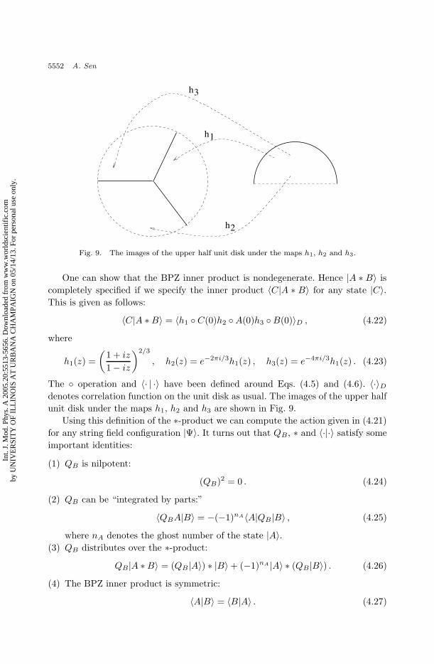
September 29, 2005 17:21 WSPC/139-IJMPA 02519
5552 A. Sen
h
h
h
1
2
3
Fig. 9. The images of the upper half unit disk under the maps h1, h2 and h3.
One can show that the BPZ inner product is nondegenerate. Hence |A ∗ B〉 is
completely specified if we specify the inner product 〈C|A ∗ B〉 for any state |C〉.This is given as follows:
〈C|A ∗B〉 = 〈h1 C(0)h2 A(0)h3 B(0)〉D , (4.22)
where
h1(z) =
(
1 + iz
1 − iz
)2/3
, h2(z) = e−2πi/3h1(z) , h3(z) = e−4πi/3h1(z) . (4.23)
The operation and 〈· | ·〉 have been defined around Eqs. (4.5) and (4.6). 〈·〉Ddenotes correlation function on the unit disk as usual. The images of the upper half
unit disk under the maps h1, h2 and h3 are shown in Fig. 9.
Using this definition of the ∗-product we can compute the action given in (4.21)
for any string field configuration |Ψ〉. It turns out that QB , ∗ and 〈·|·〉 satisfy some
important identities:
(1) QB is nilpotent:
(QB)2 = 0 . (4.24)
(2) QB can be “integrated by parts:”
〈QBA|B〉 = −(−1)nA〈A|QB |B〉 , (4.25)
where nA denotes the ghost number of the state |A〉.(3) QB distributes over the ∗-product:
QB|A ∗B〉 = (QB |A〉) ∗ |B〉 + (−1)nA |A〉 ∗ (QB |B〉) . (4.26)
(4) The BPZ inner product is symmetric:
〈A|B〉 = 〈B|A〉 . (4.27)
Int.
J. M
od. P
hys.
A 2
005.
20:5
513-
5656
. Dow
nloa
ded
from
ww
w.w
orld
scie
ntif
ic.c
omby
UN
IVE
RSI
TY
OF
ILL
INO
IS A
T U
RB
AN
A C
HA
MPA
IGN
on
05/1
4/13
. For
per
sona
l use
onl
y.
September 29, 2005 17:21 WSPC/139-IJMPA 02519
Tachyon Dynamics in Open String Theory 5553
(5) The quantity 〈A|B ∗ C〉 is cyclic:
〈A|B ∗ C〉 = 〈C|A ∗B〉 . (4.28)
(6) The ∗-product is associative:
(|A〉 ∗ |B〉) ∗ |C〉 = |A〉 ∗ (|B〉 ∗ |C〉) . (4.29)
These identities can be proved by using the general properties of the matter-ghost
BCFT, without restricting ourselves to any specific choice of the matter BCFT. We
however do need to use the fact that the matter BCFT has total central charge 26.
Using these identities one can show that the action (4.21) is invariant under an
infinitesimal gauge transformation:
δ|Φ〉 = QB |Λ〉 + |Φ〉 ∗ |Λ − |Λ〉 ∗ |Φ〉 , (4.30)
where the infinitesimal gauge transformation parameter |Λ〉 is an arbitrary state in
H0. More specifically, if |χ0,s〉 denote a set of basis states in H0, and if we expand
|Λ〉 as
|Λ〉 =∑
s
λs|χ0,s〉 , (4.31)
then the coefficients of expansion λs are infinitesimal and represent the gauge trans-
formation parameters.o The variation of the action S under the transformation
(4.30) vanishes to first order in λs.
The equations of motion obtained by requiring δS = 0 under arbitrary variation
δ|Φ〉 to first order in δ|Φ〉, gives
QB|Φ〉 + |Φ〉 ∗ |Φ〉 = 0 . (4.32)
Thus at the linearized level the equations of motion take the form
QB |Φ〉 = 0 . (4.33)
This agrees with the physical state condition (4.9). Furthermore, at the linearized
level the gauge transformation (4.30) takes the form
δ|Φ〉 = QB |Λ〉 . (4.34)
Thus equivalence under linearized gauge transformation reproduces the equivalence
relation (4.12) of the first quantized theory. This shows that gauge inequivalent
solutions of the linearized equations of motion of string theory are in one-to-one
correspondence to the physical states of the first quantized theory. This is one of
the requirements that the string field theory must satisfy.
It can be shown that the other requirement, that the S-matrix elements involving
physical external states computed using the Feynman rules of string field theory
oAgain by regarding the sum over s as a sum over a discrete index and integration over thecontinuous momentum index we can regard λs as a set of functions of the momentum alongthe D-brane, or by taking their Fourier transform, a set of functions of the coordinates along theD-brane worldvolume.
Int.
J. M
od. P
hys.
A 2
005.
20:5
513-
5656
. Dow
nloa
ded
from
ww
w.w
orld
scie
ntif
ic.c
omby
UN
IVE
RSI
TY
OF
ILL
INO
IS A
T U
RB
AN
A C
HA
MPA
IGN
on
05/1
4/13
. For
per
sona
l use
onl
y.
September 29, 2005 17:21 WSPC/139-IJMPA 02519
5554 A. Sen
reproduce the S-matrix elements computed using Polyakov prescription, is also
satisfied by the open string field theory described here.535,191,192 The computation
in string field theory requires a gauge fixing. The most commonly used gauge is the
Siegel gauge, where we require:
b0|Φ〉 = 0 . (4.35)
We shall make use of this gauge condition later.
4.3. Reformulation of the tachyon condensation conjectures in
string field theory
We shall now reformulate the three conjectures about the tachyon potential on a
bosonic D-brane in the language of string field theory. Since the conjectures involve
properties of classical solutions of open string field theory (translationally invariant
vacuum solution and lump solutions) we shall begin by reviewing certain properties
of classical solutions in open string field theory. Let |Φcl〉 denote a specific solution
of the classical equations of motion (4.32):
QB |Φcl〉 + |Φcl〉 ∗ |Φcl〉 = 0 . (4.36)
If we want to study string field theory around this classical solution, it is convenient
to define shifted field |Ψ〉 as
|Ψ〉 = |Φ〉 − |Φcl〉 , (4.37)
and rewrite the original action as
S(|Φ〉) = S(|Φcl〉) + S(|Ψ〉) , (4.38)
where
S(|Ψ〉) = − 1
g2
[
1
2〈Ψ|Q|Ψ〉 +
1
3〈Ψ|Ψ ∗ Ψ〉
]
, (4.39)
with
Q|A〉 ≡ QB |A〉 + |Φcl〉 ∗ |A〉 − (−1)nA |A〉 ∗ |Φcl〉 , (4.40)
for any state |A〉 ∈ H. One can show that as long as |Φcl〉 satisfies the equation of
motion (4.36), all the identities satisfied by QB , ∗-product and BPZ inner product
hold with QB replaced by Q. This, in turn shows that S(|Ψ〉) is invariant under a
gauge transformation:
δ|Ψ〉 = Q|Λ〉 + |Ψ〉 ∗ |Λ〉 − |Λ〉 ∗ |Ψ〉 . (4.41)
Int.
J. M
od. P
hys.
A 2
005.
20:5
513-
5656
. Dow
nloa
ded
from
ww
w.w
orld
scie
ntif
ic.c
omby
UN
IVE
RSI
TY
OF
ILL
INO
IS A
T U
RB
AN
A C
HA
MPA
IGN
on
05/1
4/13
. For
per
sona
l use
onl
y.

September 29, 2005 17:21 WSPC/139-IJMPA 02519
Tachyon Dynamics in Open String Theory 5555
From the structure of the action (4.39) and the gauge transformation law (4.41) it
follows that the spectrum of perturbative physical open string states around the
solution |Φcl〉, obtained by finding the gauge inequivalent solutions of the linearized
equations of motion derived from S(|Ψ〉), is in one-to-one correspondence with the
cohomology of Q. In other words, they are given by Eqs. (4.9) and (4.12) with QB
replaced by Q.
We are now in a position to restate the tachyon condensation conjectures in
the language of string field theory. For simplicity we shall restrict our discussion to
static Dp-branes in flat (25 + 1)-dimensional space–time, but many of the results
hold for D-branes in more general space–time background.
(1) There is a translationally invariant solution |Φ0〉 of the string field theory equa-
tions of motion:
QB|Φ0〉 + |Φ0〉 ∗ |Φ0〉 = 0 , (4.42)
such that
− 1
Vp+1S(|Φ0〉) + T p = 0 . (4.43)
Here Vp+1 is the volume of the D-brane worldvolume. Since for a space–time
independent solution the value of the action is given by −Vp+1 multiplied by
the value of the potential at |Φ0〉, (4.43) is a restatement of (2.21).
(2) Associated with the solution |Φ0〉 we have a nilpotent operator Q defined
through Eq. (4.40):
Q|A〉 ≡ QB |A〉 + |Φ0〉 ∗ |A〉 − (−1)nA |A〉 ∗ |Φ0〉 . (4.44)
Cohomology of Q represents the spectrum of physical open string states around
|Φ0〉. Since we do not expect any physical open string state around the tachyon
vacuum solution, the cohomology of Q must be trivial.
(3) ∀q such that 0 < q ≤ p, there should be a solution |Φq〉 of the equations
of motion which depends on q of the spatial coordinates and represents a D-
(p− q)-brane. The requirement that the energy per unit (p− q)-volume of this
solution agrees with the tension of the D-(p− q)-brane gives:
S(|Φq〉) − S(|Φ0〉) = −Vp−q+1T p−q . (4.45)
Note that in computing the energy of the solution we take the zero of the
energy to be at the tachyon vacuum solution, since by the first conjecture this
represents the vacuum without any D-brane. Note also that the solution |Φ0〉,which is supposed to describe the original Dp-brane, is to be identified as the
trivial solution (|Φ0〉 = 0). Thus S(|Φ0〉) = 0, and for q = 0 Eq. (4.45) reduces
to Eq. (4.43).
Int.
J. M
od. P
hys.
A 2
005.
20:5
513-
5656
. Dow
nloa
ded
from
ww
w.w
orld
scie
ntif
ic.c
omby
UN
IVE
RSI
TY
OF
ILL
INO
IS A
T U
RB
AN
A C
HA
MPA
IGN
on
05/1
4/13
. For
per
sona
l use
onl
y.
September 29, 2005 17:21 WSPC/139-IJMPA 02519
5556 A. Sen
4.4. Verification of the first conjecture
In this subsection we shall discuss verification of Eq. (4.43). For this we need to
study the component form of the action. Expanding the string field |Φ〉 in a basis
as in (4.13) and substituting it in the expression for the action (4.21), we get
S(|Φ〉) = − 1
g2
[
1
2Aαβφαφβ +
1
3Cαβγφαφβφγ
]
, (4.46)
Aαβ = 〈χ1,α|QB |χ1,β〉 ,Cαβγ = 〈h1 χ1,α(0)h2 χ1,β(0)h3 χ1,γ(0)〉D .
(4.47)
As discussed before, for a Dp-brane in flat space–time, the label α can be split
into a pair of labels — a discrete label r and a continuous momentum label kµalong directions tangential to the Dp-brane. Thus φα can be regarded as a set of
functions φr(k), and∑
α in the action can be replaced by∑
r
∫
dp+1k. The basis
states |χ1,α〉 can be thought of as the set |χ1,r(k)〉 with |χ1,r(k)〉 being a state
built on the Fock vacuum |k〉 by the action of various oscillators.
Analysis of the tachyon vacuum solution is simplified due to the fact that the
solution is translationally invariant. In momentum space this allows us to write
φr(k) = φr(2π)p+1δ(p+1)(k) . (4.48)
Thus the expansion (4.13) can be rewritten as
|Φ〉 =∑
r
φr|χ1,r〉 , (4.49)
where |χ1,r〉 ≡ |χ1,r(k = 0)〉 is a basis of zero momentum states in H1. The
component form of the action restricted to this subspace is given by
S(|Φ〉) = − 1
g2
[
1
2Arsφrφs +
1
3Crstφrφsφt
]
, (4.50)
where Ars and Crst are defined in the same way as in (4.47), with the state χ1,α,
etc. replaced by χ1,r. Note however that since |χ1,s〉 carries zero momentum, both
Ars and Crst carry explicit factors of Vp+1 due to the normalization condition (4.18),
and hence it will be more convenient for our analysis to define new coefficients Ars
and Crst by removing this volume factor:
Ars = Vp+1Ars , Crst = Vp+1Crst , (4.51)
Ars = 〈χ1,r|QB |χ1,s〉′ , Crst = 〈χ1,r|χ1,s ∗ χ1,t〉′ , (4.52)
where 〈·〉′ has been defined in (4.19). The action (4.50) may now be written as
S(|Φ〉) = − 1
g2Vp+1V(|Φ〉) , (4.53)
where
V(|Φ〉) =1
2Arsφrφs +
1
3Crstφrφsφt =
1
2〈Φ|QB |Φ〉′ +
1
3〈Φ|Φ ∗ Φ〉′ . (4.54)
Int.
J. M
od. P
hys.
A 2
005.
20:5
513-
5656
. Dow
nloa
ded
from
ww
w.w
orld
scie
ntif
ic.c
omby
UN
IVE
RSI
TY
OF
ILL
INO
IS A
T U
RB
AN
A C
HA
MPA
IGN
on
05/1
4/13
. For
per
sona
l use
onl
y.
September 29, 2005 17:21 WSPC/139-IJMPA 02519
Tachyon Dynamics in Open String Theory 5557
Conjecture 1, given in (4.43) can now be rewritten as
1
g2V(|Φ0〉) + T p = 0 . (4.55)
We can bring this into a more suggestive form by expressing T p in terms of g2.
An expression for T p in terms of closed string coupling constant gs has been given
in (2.20), but we would like to express this in terms of the open string coupling
constant g. This can be done in many ways. One way of doing this is to examine
the open string field theory action carefully to determine the inertial mass per
unit volume of the D-p-brane and identify this with T p. This analysis yields the
relation:471
T p =1
2π2g2. (4.56)
Substituting this into (4.55) we get
2π2V(|Φ0) + 1 = 0 . (4.57)
Thus our task is to begin with the V(|Φ〉) given in (4.54), find a local minimum
of this expression by varying the various coefficients φr, and show that the value of
V(|Φ〉) at the local minimum satisfies (4.57). Several simplifications occur in this
computation which allows us to restrict |Φ〉 to a subspace smaller than the space
of all zero momentum states in H1. First of all it turns out that the structure
of S(|Φ〉) allows a consistent truncation of the action where we restrict |Φ〉 to
linear combination of states created from the vacuum |0〉 by the action of the ghost
oscillators and matter Virasoro generators,471 instead of letting |Φ〉 be an arbitrary
linear combination of matter and ghost oscillators acting on the vacuum.p We shall
call the subspace generated by these states the universal subspace.q Second, the
V(|Φ〉) has a Z2 symmetry known as the twist invariance, under which
|Φ〉 → (−1)L0+1|Φ〉 , (4.58)
where Ln’s denote the total Virasoro generators of the matter-ghost BCFT. If we
denote by “twist” the (−1)L0+1 eigenvalue of a state, then this Z2 symmetry allows
us to restrict |Φ〉 to twist even sector in our search for the tachyon vacuum solution.
Finally, due to the gauge invariance of the action, we can impose a gauge condition.
One can show that in the twist even sector the Siegel gauge (4.35) is a good choice
of gauge around the point |Φ〉 = 0.472 Thus to begin with, we could look for a
pConsistent truncation of the action means that if we restrict |Φ〉 to this subspace, then theequations of motion associated with the components of |Φ〉 outside this subspace are automaticallysatisfied.qOnce we restrict |Φ〉 to the universal subspace, all the conformal field theory correlation functionswhich go into the computation of V(|Φ〉) are independent of the specific choice of the conformalfield theory used for this computation. This shows that once we have established (4.57) for someunstable D-brane in some closed string background, it proves the first conjecture for any D-branein any closed string background in the bosonic string theory.471 A similar argument also worksfor the superstring theory.
Int.
J. M
od. P
hys.
A 2
005.
20:5
513-
5656
. Dow
nloa
ded
from
ww
w.w
orld
scie
ntif
ic.c
omby
UN
IVE
RSI
TY
OF
ILL
INO
IS A
T U
RB
AN
A C
HA
MPA
IGN
on
05/1
4/13
. For
per
sona
l use
onl
y.
September 29, 2005 17:21 WSPC/139-IJMPA 02519
5558 A. Sen
solution |Φ0〉 in the Siegel gauge, and after we have obtained the solution, verify
that the Siegel gauge is still a good choice of gauge near the solution |Φ0〉. We shall
denote by H1 the restricted subspace of H1 satisfying all these requirements.r
Let us define the level of a state |s〉 to be the difference between the L0 eigenvalue
h of |s〉 and the L0 eigenvalue of the state c1|0〉 representing the zero momentum
tachyon. Since the latter state has L0 eigenvalue −1, the level of |s〉 is given by
(1 + h). Thus, for example, c1|0〉 has level 0, c−1|0〉 and c1L(m)−2 |0〉 has level 2, etc.
Using this definition we can partially order the zero momentum basis states in the
order of increasing level. Thus for example in H1, |Φ〉 can be expanded as
|Φ〉 = φ0c1|0〉 + φ1c−1|0〉 + φ2L(m)−2 c1|0〉 + · · · , (4.59)
where · · · involves states of level 4 and higher. Let us now make a drastic approxi-
mation where we set all the coefficients other than that of level zero state c1|0〉 to
zero. Substituting this into (4.54) we get
V(φ0) =1
2φ2
0〈0|c−1QBc1|0〉′ +1
3φ3
0〈h1 c(0)h2 c(0)h3 c(0)〉′D . (4.60)
The relevant correlation functions can be easily evaluated and give
V(φ0) = −1
2φ2
0 +1
3
(
3√
3
4
)3
φ30 . (4.61)
This has a local minimum at φ0 = (4/3√
3)3, and at this minimum,
2π2V(φ0) = −(2π2)(4/3√
3)6/6 ' −0.684 . (4.62)
This is about 68% of the conjectured answer −1 given in (4.57).
This is the beginning of a systematic approximation scheme known as the level
truncation.307–309,472,376,169 We define the level of a coefficient φr to be the level
of the state |χ1,r〉 that it multiplies in the expansion of |Φ〉. We now define a
level (M,N) approximation to V(|Φ〉) as follows:
(1) Keep all fields φr of level ≤M .
(2) Keep all terms in the action for which the sum of the levels of all fields in that
term is ≤ N . Thus for example at level (2, 4) we shall include interaction terms
of the form 0–0–0, 0–0–2, 0–2–2 but ignore interaction terms of the form 2–2–2.
(3) This gives an expression for V(|Φ〉) involving finite number of fields and finite
number of terms. We find a (local) minimum of this V(|Φ〉) and evaluate the
value of V(|Φ〉) at this minimum.
rIn the Siegel gauge the action has an SU(1, 1) invariance495,555 which allows us to further restrict|Φ〉 to SU(1, 1) singlet subspace,555 but this has not so far been used effectively in simplifying theanalysis. Nevertheless, once the solution has been found, one can explicitly check that the solutionis an SU(1, 1) singlet.555
Int.
J. M
od. P
hys.
A 2
005.
20:5
513-
5656
. Dow
nloa
ded
from
ww
w.w
orld
scie
ntif
ic.c
omby
UN
IVE
RSI
TY
OF
ILL
INO
IS A
T U
RB
AN
A C
HA
MPA
IGN
on
05/1
4/13
. For
per
sona
l use
onl
y.
September 29, 2005 17:21 WSPC/139-IJMPA 02519
Tachyon Dynamics in Open String Theory 5559
This defines the level (M,N) approximation to V(|Φ0〉). In order for this to be a
sensible approximation scheme, we need to ensure that the answer converges as we
increase the values of M , N . In actual practice this method converges quite rapidly.
For example the value of −2π2V(|Φ0〉) in level (L, 2L) approximation increases
monotonically towards 1 as we increase the value of L up to L = 10, reaching
the value 0.9991 at L = 10.376 However beyond level 12 the value of −2π2V(|Φ0〉)overshoots the expected value 1, and continue to increase with L till about level
18 approximation.169 Nevertheless analysis of the tachyon potential obtained by
integrating out all fields other than φ0 shows that −2π2V(|Φ0〉) eventually turns
back and approaches the expected value 1 from above.519,169
Since the solution is constructed in the Siegel gauge, we need to verify that Siegel
gauge is a valid gauge choice for this solution. Operationally what this amounts to
is the following. In arriving at the solution, we have made sure that the variation
δS of the action under a variation δ|Φ〉 vanishes to first order in δ|Φ〉 around the
solution, provided δ|Φ〉 satisfies the Siegel gauge condition b0δ|Φ〉 = 0. In order to
check that the solution satisfies the full string field theory equations of motion we
need to make sure that δS vanishes to first order in δ|Φ〉 even if δ|Φ〉 does not
satisfy the Siegel gauge condition. To check this, we can simply take the first order
variation of V(|Φ〉) with respect to components of |Φ〉 which violate Siegel gauge
condition and verify that these derivatives vanish when evaluated in the background
of the solution |Φ0〉 found using the level truncation scheme. This has been checked
explicitly in Refs. 239 and 169.
4.5. Verification of the second and third conjectures
We shall now briefly discuss the verification of the second and the third conjectures.
Of these the analysis of the third conjecture, Eq. (4.45), proceeds in a way very
similar to that of the first conjecture.113,377,114,378 The main difference is that since
the solution depends on q of the spatial coordinates, we can no longer restrict |Φ〉 to
be in the zero momentum sector for finding the solution |Φq〉; instead we must allow
|Φ〉 to carry momentum along these q directions. The analysis can be simplified by
compactifying the q directions along which we want the lump to form. This makes
the momenta in these directions discrete, and as a result |Φ〉 can still be expanded
in the discrete basis.
The explicit construction of the solution now proceeds via a modified level trun-
cation scheme where the level of a state, given by (L0 + 1), includes not only the
oscillator contribution but also the contribution to L0 due to the momentum along
the compact directions. The level (M,N) approximation is defined exactly as before,
and for finite (M,N) we still have a finite number of variables with respect to which
we need to extremize the action. For q = 1 the result converges fast towards the
expected value as we increase the level of approximation.377 In particular, the ten-
sion of the soliton becomes independent of the radius of compactification, as is
expected of a D-brane whose transverse direction is compactified. The convergence
Int.
J. M
od. P
hys.
A 2
005.
20:5
513-
5656
. Dow
nloa
ded
from
ww
w.w
orld
scie
ntif
ic.c
omby
UN
IVE
RSI
TY
OF
ILL
INO
IS A
T U
RB
AN
A C
HA
MPA
IGN
on
05/1
4/13
. For
per
sona
l use
onl
y.
September 29, 2005 17:21 WSPC/139-IJMPA 02519
5560 A. Sen
is also reasonably good for q = 2.114,378 Today the best available results for the
tension of the codimension q lump solution for q = 1 and q = 2 differ from their
conjectured values by 1% (Ref. 377) and 13% (Refs. 114 and 378) respectively. For
larger values of q the number of fields below a given level increases rapidly, slowing
down the convergence. The number of fields also increases rapidly as we increase the
radius of compactification since states carrying different momenta become closely
spaced in level. Nevertheless the analysis has been done for different radii, and the
tension of the resulting lump solution has been shown to be independent of the
radius to a very good approximation as is expected of a D-brane.
All the lump solutions described above have been constructed in the Siegel
gauge. For the codimension one lump, the validity of the Siegel gauge choice has
been tested in Ref. 389.
For verifying Conjecture 2, we need to check that Q defined in Eq. (4.44) has
trivial cohomology. This can be done as follows:138
(1) Take the best available value of |Φ0〉 obtained using the level truncation scheme
and construct Q from there using Eq. (4.44).
(2) Construct solutions of Q|A〉 = 0 by taking |A〉 to be arbitrary linear combina-
tions of states up to a certain level.
(3) Show that for every such |A〉, there is a state |B〉 such that |A〉 = Q|B〉.
There is however a further complication due to the fact that |Φ0〉 obtained in the
level truncation scheme is only an approximate solution of the equations of motion,
and as a result Q defined in Eq. (4.44) does not square to zero exactly when we use
this approximate value of |Φ0〉. Hence a state |A〉 = Q |B〉 does not satisfy Q|A〉 = 0
exactly. We can circumvent this problem by using an approximate rather than an
exact analysis of the Q-cohomology.138 Given a state |A〉 satisfying Q|A〉 = 0, we
check if there is a state |B〉 such that the ratio of the norm of (|A〉 −Q|B〉) to the
norm of |A〉 can be made small. Of course there is no natural norm in the space
of the string field since the BPZ inner product of ghost number 1 state with itself
vanishes by ghost charge conservation, but we could use several different artificial
norms (e.g. by explicitly inserting a factor of c0 in the BPZ inner product), and
check if the final conclusion is sensitive to the choice of the norm. It was found in
Ref. 138 that if we carry out this analysis in a subspace which includes string states
up to a given oscillator level L, and carrying momentum k with |k2| ≤ L, then
all Q closed states are also Q-exact to within 1% accuracy. This gives numerical
evidence for the absence of the physical open string states around the tachyon
vacuum.
A somewhat different approach to this problem has been suggested in Ref. 194.
Various other aspects of tachyon condensation in bosonic open string field theory
have been discussed in Refs. 517, 221, 113, 437, 110, 473, 518, 453, 105, 454, 240,
147, 139, 140, 366, 333, 401, 511, 116, 455, 167, 512, 288, 513, 514, 410, 489, 546
and 276.
Int.
J. M
od. P
hys.
A 2
005.
20:5
513-
5656
. Dow
nloa
ded
from
ww
w.w
orld
scie
ntif
ic.c
omby
UN
IVE
RSI
TY
OF
ILL
INO
IS A
T U
RB
AN
A C
HA
MPA
IGN
on
05/1
4/13
. For
per
sona
l use
onl
y.
September 29, 2005 17:21 WSPC/139-IJMPA 02519
Tachyon Dynamics in Open String Theory 5561
4.6. Superstring field theory
In this subsection we shall briefly discuss the use of superstring field theory in veri-
fying the conjectured properties of the tachyon potential in superstring theory. For
this discussion we shall use the Berkovits version of superstring field theory.54,55,58,59
An alternative approach to this problem based on various cubic versions of super-
string field theory536,17,18,434 has been proposed in Refs. 118, 19 and 20, but we
shall not discuss it here.
We shall begin by reviewing the formulation of first quantized open superstring
theory on a non-BPS D-brane44,465,466 in a convention which will facilitate the
formulation of superstring field theory.54,55,57 We restrict ourselves to the Neveu–
Schwarz (NS) sector of the theory, since only the bosonic fields arising in this sector
are involved in the construction of the classical solutions describing the tachyon
vacuum and various lower dimensional D-branes. In the first quantized formulation
the bulk worldsheet theory is given by a c = 15 superconformal field theory together
with a set of anticommuting ghosts b, c, b, c and commuting ghosts β, γ, β, γ. The
fields β, γ can be replaced by a pair of fermions ξ, η, and a scalar φg through the
relations158
β = ∂ξe−φg , γ = ηeφg . (4.63)
ξ and η have dimensions (0, 0) and (1, 0) respectively, whereas φg is a chiral scalar
field with background charge so that 〈eqφg(0)〉D is nonzero only for q = −2. There
are similar relations involving the antiholomorphic fields. The fields ξ, η and φg are
normalized such that
ξ(z)η(w) ' 1
z − w, ∂φg(z)∂φg(w) ' − 1
(z − w)2, (4.64)
with a similar relation among the antiholomorphic components. Since the open
string vertex operators will involve the boundary values of various fields, and since
on the boundary the holomorphic and the antiholomorphic ghost fields are set equal,
we shall not need to refer to the antiholomorphic ghost fields explicitly. The ghost
number (ng) and the picture number (np) assignments of various fields are defined
as follows:
b : ng = −1 , np = 0 , c : ng = 1 , np = 0 ,
eqφg : ng = 0 , np = q ,
ξ : ng = −1 , np = 1 , η : ng = 1 , np = −1 .
(4.65)
The matter fields as well as the SL(2, R) invariant vacuum carry zero ghost and
picture number. The GSO operator is given by
(−1)F (−1)q , (4.66)
where F denotes the worldsheet fermion number of the matter fields, and q denotes
the φg momentum.
Int.
J. M
od. P
hys.
A 2
005.
20:5
513-
5656
. Dow
nloa
ded
from
ww
w.w
orld
scie
ntif
ic.c
omby
UN
IVE
RSI
TY
OF
ILL
INO
IS A
T U
RB
AN
A C
HA
MPA
IGN
on
05/1
4/13
. For
per
sona
l use
onl
y.
September 29, 2005 17:21 WSPC/139-IJMPA 02519
5562 A. Sen
The physical open string states are states of ghost number 1, with each physical
state having different representations in different picture numbers.158 Furthermore,
they are required to satisfy the following conditions:
(1) |φ〉 is BRST invariant:
QB |φ〉 = 0 , (4.67)
where QB is the BRST charge defined as
QB =
∮
dz jB(z)
=
∮
dzc(Tm + Tξη + Tφg)
+ c∂cb+ ηeφgGm − η∂ηe2φgb , (4.68)
Tξη = ∂ξη , Tφg= −1
2∂φg∂φg − ∂2φg . (4.69)
Tm is the matter stress tensor and Gm is the matter superconformal generator.
(2) Two states |φ〉 and |φ′〉 are considered to be equivalent if they differ by QB |Λ〉for some state |Λ〉:
|φ〉 ≡ |φ〉 +QB |Λ〉 . (4.70)
(3) |φ〉 can be either GSO odd or GSO even. The vertex operators of GSO even
states are accompanied by Chan–Paton factors I (I being the 2 × 2 identity
matrix), whereas vertex operators of GSO odd states are accompanied by Chan–
Paton factor σ1. This rule is inherited from the parent brane–antibrane system
for which the GSO even states carry Chan–Paton factors I and σ3 and GSO
odd states carry Chan–Paton factors σ1 and σ2. The (−1)FL projection removes
the states carrying Chan–Paton factors σ2 and σ3.
(4) The field ξ appears in the vertex operators for physical states only through
its derivatives. In terms of the state |φ〉 it means that |φ〉 is annihilated by
η0, where ηn, ξn denote the modes of the fields η and ξ defined through the
expansion
η(z) =∑
n
ηnz−n−1 , ξ(z) =
∑
n
ξnz−n . (4.71)
This condition given in item (4) above gives what is known as the small picture
representation of the physical states.53 For the formulation of the superstring field
theory it is more convenient to use the big picture54,55 where given a state |φ〉satisfying the conditions given above, we use the state ξ0|φ〉 to represent the same
physical state.s In terms of vertex operators this corresponds to multiplying the
vertex operator in the small picture representation by ξ. Thus for example a repre-
sentation of the on-shell tachyon vertex operator carrying momentum k in the small
sConsequently a physical state in the big picture is annihilated by QBη0 instead of QB .
Int.
J. M
od. P
hys.
A 2
005.
20:5
513-
5656
. Dow
nloa
ded
from
ww
w.w
orld
scie
ntif
ic.c
omby
UN
IVE
RSI
TY
OF
ILL
INO
IS A
T U
RB
AN
A C
HA
MPA
IGN
on
05/1
4/13
. For
per
sona
l use
onl
y.
September 29, 2005 17:21 WSPC/139-IJMPA 02519
Tachyon Dynamics in Open String Theory 5563
picture is ce−φgeik·X ⊗σ1. The same vertex operator in the big picture will be given
by ξce−φgeik·X ⊗ σ1. According to our convention given in (4.65) the small picture
representation is in picture number −1 whereas the big picture representation is in
picture number 0.
Let us now turn to the construction of open superstring field theory. As in
the case of bosonic string theory, a general open string field configuration Φ is
represented by a state in the worldsheet boundary conformal field theory which do
not satisfy all the requirements of a physical state. It turns out that the choice of
a general off-shell field configuration in superstring field theory is as follows. In the
NS sector it contains two components, a GSO even component Φ+ accompanied
by a Chan–Paton factor I and a GSO odd component Φ− accompanied by the
Chan–Paton factor σ1. Both Φ+ and Φ− are required to have picture number 0 and
ghost number 0. Thus we can writet
Φ = Φ+ ⊗ I + Φ− ⊗ σ1 . (4.72)
The string field theory action to be given below will involve calculating correla-
tion functions involving the vertex operators Φ±. In manipulating these correlation
functions, we need to keep in mind that the string field components in the NS sector
are always Grassman even, whereas the open string vertex operators which these
components multiply in the expression of Φ± may be Grassman even or Grassman
odd depending on the worldsheet fermion number carried by the vertex operator.
In particular the fermion ψµ associated with the matter BCFT, and b, c, ξ, η and
eqφg for odd q are Grassman odd fields. Using Eqs. (4.65), (4.66) one can then
show that Φ+ is Grassman even whereas Φ− is Grassman odd. In particular, the
zero momentum tachyon vertex operator ξce−φg ⊗ σ1 is GSO odd and Grassman
odd. Note the extra factor of ξ in the tachyon vertex operator compared to the
conventions used in Sec. 3. This is due to the fact that we are using the big picture.
The BRST charge QB acting on the string field and the operator η0 is defined by
QB = QB ⊗ σ3 , η0 = η0 ⊗ σ3 . (4.73)
Also, given a set of open string vertex operators A1, . . . An on a non-BPS Dp-brane,
we define
〈〈A1 . . . An〉〉 = Tr⟨
f(n)1 A1(0) · · · f (n)
n An(0)⟩
D, (4.74)
where the trace is over the internal CP matrices, and
f(n)k (z) = e
2πi(k−1)n
(
1 + iz
1 − iz
)2/n
for n ≥ 1 . (4.75)
〈·〉D denotes correlation function on a unit disk as usual.
tWe shall adopt the convention that fields or operators with internal CP factors included aredenoted by symbols with a hat on them, and fields or operators without internal CP factorsincluded are denoted by symbols without a hat.
Int.
J. M
od. P
hys.
A 2
005.
20:5
513-
5656
. Dow
nloa
ded
from
ww
w.w
orld
scie
ntif
ic.c
omby
UN
IVE
RSI
TY
OF
ILL
INO
IS A
T U
RB
AN
A C
HA
MPA
IGN
on
05/1
4/13
. For
per
sona
l use
onl
y.
September 29, 2005 17:21 WSPC/139-IJMPA 02519
5564 A. Sen
In terms of these quantities the open superstring field theory action on a non-
BPS D-brane can be written as,56,57
S =1
4g2
⟨⟨
(
e−ΦQBeΦ)(
e−Φη0eΦ)
−∫ 1
0
ds(
e−sΦ∂sesΦ)(
e−sΦQBesΦ)
,(
e−sΦη0esΦ)
⟩⟩
, (4.76)
where we have divided the overall normalization by a factor of two in order to
compensate for the trace operation on the internal matrices. s in the second term
is just an integration parameter. By expanding the various exponentials in a Taylor
series expansion, and explicitly carrying out the s integral for each term one can
represent the action as a power series expansion in the string field. This is given in
Eq. (4.81).
Equation (4.76) can be shown to be invariant under the infinitesimal gauge
transformation56
δeΦ = (QBΩ)eΦ + eΦ(η0Ω′) , (4.77)
where the infinitesimal gauge transformation parameters Ω and Ω′ are states with
(ng , np) values (−1, 0) and (−1, 1) respectively. The internal CP indices carried by
the gauge parameters are as follows:
Ω = Ω+ ⊗ σ3 + Ω− ⊗ iσ2 , Ω′ = Ω′+ ⊗ σ3 + Ω′
− ⊗ iσ2 . (4.78)
The GSO even Ω+, Ω′+ are Grassmann odd, while the GSO odd Ω−, Ω′
− are Grass-
mann even. The proof of invariance of (4.76) under (4.77) can be carried out by
straightforward algebraic manipulations.56,57
An analysis similar to that in the case of bosonic string theory shows that
with the normalization we have used here, the tension of the non-BPS Dp-brane is
given by
T p =1
2π2g2. (4.79)
Thus in order to prove the first conjecture about the tachyon potential we need to
show the existence of a solution |Φ0〉 of the equations of motion derived from the
string field theory action, such that
S(|Φ0〉) = Vp+11
2π2g2, (4.80)
where Vp+1 is the volume of the Dp-brane worldvolume.
The calculation proceeds as in the case of bosonic string theory using the level
truncation scheme.56,57 For this we need to first expand the action (4.76) in a power
series expansion in the string field. This gives
S =1
2g2
∞∑
M,N=0
1
(M +N + 2)!
(
M +N
N
)
(−1)N⟨⟨
(QBΦ)ΦM (η0Φ)ΦN⟩⟩
. (4.81)
Int.
J. M
od. P
hys.
A 2
005.
20:5
513-
5656
. Dow
nloa
ded
from
ww
w.w
orld
scie
ntif
ic.c
omby
UN
IVE
RSI
TY
OF
ILL
INO
IS A
T U
RB
AN
A C
HA
MPA
IGN
on
05/1
4/13
. For
per
sona
l use
onl
y.
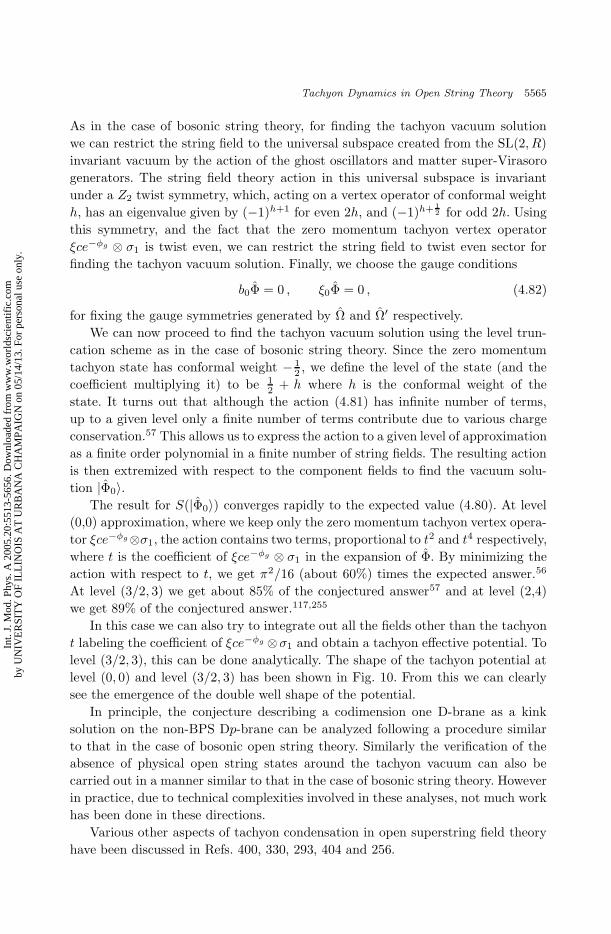
September 29, 2005 17:21 WSPC/139-IJMPA 02519
Tachyon Dynamics in Open String Theory 5565
As in the case of bosonic string theory, for finding the tachyon vacuum solution
we can restrict the string field to the universal subspace created from the SL(2, R)
invariant vacuum by the action of the ghost oscillators and matter super-Virasoro
generators. The string field theory action in this universal subspace is invariant
under a Z2 twist symmetry, which, acting on a vertex operator of conformal weight
h, has an eigenvalue given by (−1)h+1 for even 2h, and (−1)h+ 12 for odd 2h. Using
this symmetry, and the fact that the zero momentum tachyon vertex operator
ξce−φg ⊗ σ1 is twist even, we can restrict the string field to twist even sector for
finding the tachyon vacuum solution. Finally, we choose the gauge conditions
b0Φ = 0 , ξ0Φ = 0 , (4.82)
for fixing the gauge symmetries generated by Ω and Ω′ respectively.
We can now proceed to find the tachyon vacuum solution using the level trun-
cation scheme as in the case of bosonic string theory. Since the zero momentum
tachyon state has conformal weight − 12 , we define the level of the state (and the
coefficient multiplying it) to be 12 + h where h is the conformal weight of the
state. It turns out that although the action (4.81) has infinite number of terms,
up to a given level only a finite number of terms contribute due to various charge
conservation.57 This allows us to express the action to a given level of approximation
as a finite order polynomial in a finite number of string fields. The resulting action
is then extremized with respect to the component fields to find the vacuum solu-
tion |Φ0〉.The result for S(|Φ0〉) converges rapidly to the expected value (4.80). At level
(0,0) approximation, where we keep only the zero momentum tachyon vertex opera-
tor ξce−φg⊗σ1, the action contains two terms, proportional to t2 and t4 respectively,
where t is the coefficient of ξce−φg ⊗ σ1 in the expansion of Φ. By minimizing the
action with respect to t, we get π2/16 (about 60%) times the expected answer.56
At level (3/2, 3) we get about 85% of the conjectured answer57 and at level (2,4)
we get 89% of the conjectured answer.117,255
In this case we can also try to integrate out all the fields other than the tachyon
t labeling the coefficient of ξce−φg ⊗σ1 and obtain a tachyon effective potential. To
level (3/2, 3), this can be done analytically. The shape of the tachyon potential at
level (0, 0) and level (3/2, 3) has been shown in Fig. 10. From this we can clearly
see the emergence of the double well shape of the potential.
In principle, the conjecture describing a codimension one D-brane as a kink
solution on the non-BPS Dp-brane can be analyzed following a procedure similar
to that in the case of bosonic open string theory. Similarly the verification of the
absence of physical open string states around the tachyon vacuum can also be
carried out in a manner similar to that in the case of bosonic string theory. However
in practice, due to technical complexities involved in these analyses, not much work
has been done in these directions.
Various other aspects of tachyon condensation in open superstring field theory
have been discussed in Refs. 400, 330, 293, 404 and 256.
Int.
J. M
od. P
hys.
A 2
005.
20:5
513-
5656
. Dow
nloa
ded
from
ww
w.w
orld
scie
ntif
ic.c
omby
UN
IVE
RSI
TY
OF
ILL
INO
IS A
T U
RB
AN
A C
HA
MPA
IGN
on
05/1
4/13
. For
per
sona
l use
onl
y.
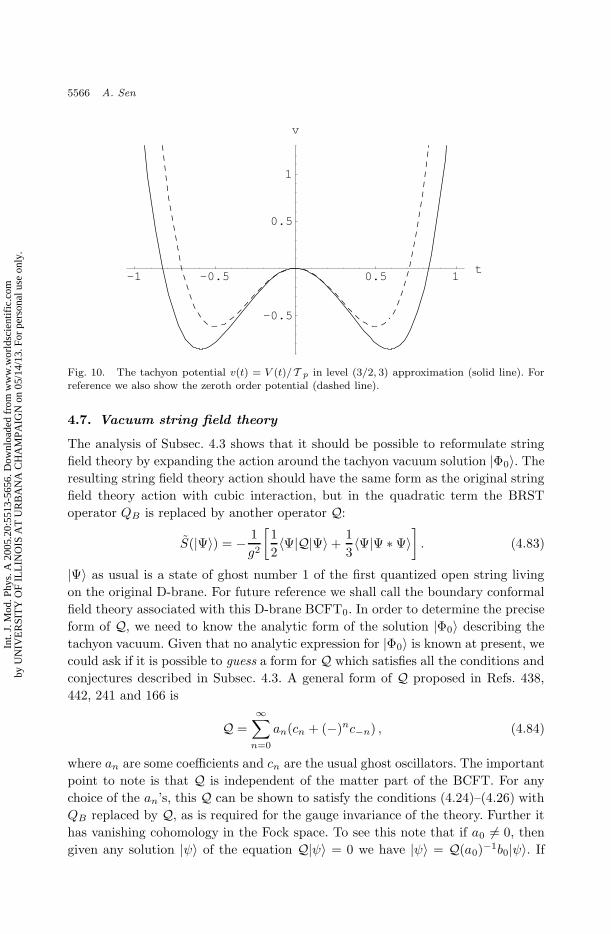
September 29, 2005 17:21 WSPC/139-IJMPA 02519
5566 A. Sen
-1 -0.5 0.5 1t
-0.5
0.5
1
v
Fig. 10. The tachyon potential v(t) = V (t)/T p in level (3/2, 3) approximation (solid line). Forreference we also show the zeroth order potential (dashed line).
4.7. Vacuum string field theory
The analysis of Subsec. 4.3 shows that it should be possible to reformulate string
field theory by expanding the action around the tachyon vacuum solution |Φ0〉. The
resulting string field theory action should have the same form as the original string
field theory action with cubic interaction, but in the quadratic term the BRST
operator QB is replaced by another operator Q:
S(|Ψ〉) = − 1
g2
[
1
2〈Ψ|Q|Ψ〉 +
1
3〈Ψ|Ψ ∗ Ψ〉
]
. (4.83)
|Ψ〉 as usual is a state of ghost number 1 of the first quantized open string living
on the original D-brane. For future reference we shall call the boundary conformal
field theory associated with this D-brane BCFT0. In order to determine the precise
form of Q, we need to know the analytic form of the solution |Φ0〉 describing the
tachyon vacuum. Given that no analytic expression for |Φ0〉 is known at present, we
could ask if it is possible to guess a form for Q which satisfies all the conditions and
conjectures described in Subsec. 4.3. A general form of Q proposed in Refs. 438,
442, 241 and 166 is
Q =
∞∑
n=0
an(cn + (−)nc−n) , (4.84)
where an are some coefficients and cn are the usual ghost oscillators. The important
point to note is that Q is independent of the matter part of the BCFT. For any
choice of the an’s, this Q can be shown to satisfy the conditions (4.24)–(4.26) with
QB replaced by Q, as is required for the gauge invariance of the theory. Further it
has vanishing cohomology in the Fock space. To see this note that if a0 6= 0, then
given any solution |ψ〉 of the equation Q|ψ〉 = 0 we have |ψ〉 = Q(a0)−1b0|ψ〉. If
Int.
J. M
od. P
hys.
A 2
005.
20:5
513-
5656
. Dow
nloa
ded
from
ww
w.w
orld
scie
ntif
ic.c
omby
UN
IVE
RSI
TY
OF
ILL
INO
IS A
T U
RB
AN
A C
HA
MPA
IGN
on
05/1
4/13
. For
per
sona
l use
onl
y.
September 29, 2005 17:21 WSPC/139-IJMPA 02519
Tachyon Dynamics in Open String Theory 5567
a0 = 0, but am 6= 0 for some m, we can write |ψ〉 = 12am
Q((−1)mbm − b−m)|ψ〉.Hence |ψ〉 is Q trivial.
It now remains to find the classical solutions predicted by the first and the third
conjecture in this field theory. Clearly the tachyon vacuum solution corresponds
to the configuration |Ψ〉 = 0. Thus the nontrivial solution we need to look for are
those describing various D-branes, including the original D-brane associated with
BCFT0. In order to find them, we look for classical solutions of the form
Ψ = Ψg ⊗ Ψm , (4.85)
where Ψg denotes a state obtained by acting with the ghost oscillators on the
SL(2, R) invariant vacuum of the ghost sector of BCFT0, and Ψm is a state obtained
by acting with matter vertex operators on the SL(2, R) invariant vacuum of the
matter sector of BCFT0. If we denote by ∗g and ∗m the star product in the ghost
and matter sector respectively, the equations of motion
QΨ + Ψ ∗ Ψ = 0 (4.86)
factorize as
QΨg = −KΨg ∗g Ψg , (4.87)
and
Ψm = K−1Ψm ∗m Ψm , (4.88)
where K is an arbitrary constant that can be changed by scaling ψg and ψm in
opposite directions. We further assume that the ghost part Ψg is universal for all
D-p-brane solutions. Under this assumption the ratio of energies associated with two
different D-brane solutions, with matter parts Ψ′m and Ψm respectively, is given by
E ′
E =S(Ψg ⊗ Ψ′
m)
S(Ψg ⊗ Ψm)=
〈Ψ′m|Ψ′
m〉m〈Ψm|Ψm〉m
, (4.89)
with 〈·|·〉m denoting BPZ inner product in the matter BCFT. Thus the ghost part
drops out of this calculation. Equation (4.88) for the matter part tells us that
|Ψm〉 is a projector under the ∗-product in the matter sector up to a constant of
proportionality.
General methods for constructing such projectors have been developed in
Refs. 310, 439, 440, 209, 441, 210 and 168. Let BCFT denote some boundary confor-
mal field theory with the same bulk worldsheet action as BCFT0, i.e. both BCFT
and BCFT0 represent D-branes in the same space–time background. Consider now
a state∣
∣ΨBCFTm
⟩
in the matter part of BCFT0, defined through the relation:u
〈ΨBCFTm |φ〉 = 〈f φ(0)〉′BCFT (4.90)
uNote that once we have chosen the reference BCFT0, the string field |Ψ〉 is always a state inBCFT0 even if it describes a D-brane associated with another BCFT.
Int.
J. M
od. P
hys.
A 2
005.
20:5
513-
5656
. Dow
nloa
ded
from
ww
w.w
orld
scie
ntif
ic.c
omby
UN
IVE
RSI
TY
OF
ILL
INO
IS A
T U
RB
AN
A C
HA
MPA
IGN
on
05/1
4/13
. For
per
sona
l use
onl
y.
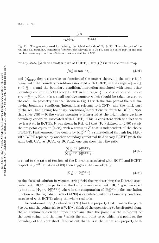
September 29, 2005 17:21 WSPC/139-IJMPA 02519
5568 A. Sen
−π/4−ε π/4+εφof
Fig. 11. The geometry used for defining the right-hand side of Eq. (4.90). The thin part of thereal line has boundary conditions/interactions relevant to BCFT0, and the thick part of the realline has boundary conditions/interactions relevant to BCFT.
for any state |φ〉 in the matter part of BCFT0. Here f(ξ) is the conformal map
f(ξ) = tan−1 ξ , (4.91)
and 〈·〉′BCFT denotes correlation function of the matter theory on the upper half-
plane, with the boundary condition associated with BCFT0 in the range −π4 − ε ≤
x ≤ π4 + ε and the boundary condition/interaction associated with some other
boundary conformal field theory BCFT in the range π4 + ε < x < ∞ and −∞ <
x < −π4 − ε. Here ε is a small positive number which should be taken to zero at
the end. The geometry has been shown in Fig. 11 with the thin part of the real line
having boundary conditions/interactions relevant to BCFT0, and the thick part
of the real line having boundary conditions/interactions relevant to BCFT. Note
that since f(0) = 0, the vertex operator φ is inserted at the origin where we have
boundary condition associated with BCFT0. This is consistent with the fact that
|φ〉 is a state in BCFT0. It was shown in Ref. 441 that |Ψm〉 defined in (4.90) satisfy
the projector equation (4.88), with a constant K that is independent of the choice
of BCFT. Furthermore, if we denote by |ΨBCFT′
m 〉 a state defined through Eq. (4.90)
with BCFT replaced by another boundary conformal field theory BCFT′ (with the
same bulk CFT as BCFT or BCFT0), one can show that the ratio
〈ΨBCFTm |ΨBCFT
m 〉〈ΨBCFT′
m |ΨBCFT′
m 〉 , (4.92)
is equal to the ratio of tensions of the D-branes associated with BCFT and BCFT′
respectively.441 Equation (4.89) then suggests that we identify
|Ψg〉 × |ΨBCFTm 〉 (4.93)
as the classical solution in vacuum string field theory describing the D-brane asso-
ciated with BCFT. In particular the D-brane associated with BCFT0 is described
by the state |Ψg〉× |ΨBCFT0m 〉 where in the computation of |ΨBCFT0
m 〉 the correlation
function on the right-hand side of (4.90) is calculated with the boundary condition
associated with BCFT0 along the whole real axis.
The conformal map f defined in (4.91) has the property that it maps the point
i to ∞, and the points ±1 to ±π4 . If we think of the open string to be situated along
the unit semi-circle on the upper half-plane, then the point i is the mid-point of
the open string, and the map f sends the mid-point to ∞ which is a point on the
boundary of the worldsheet. It turns out that this is the important property that
Int.
J. M
od. P
hys.
A 2
005.
20:5
513-
5656
. Dow
nloa
ded
from
ww
w.w
orld
scie
ntif
ic.c
omby
UN
IVE
RSI
TY
OF
ILL
INO
IS A
T U
RB
AN
A C
HA
MPA
IGN
on
05/1
4/13
. For
per
sona
l use
onl
y.
September 29, 2005 17:21 WSPC/139-IJMPA 02519
Tachyon Dynamics in Open String Theory 5569
makes the state |ΨBCFTm 〉 into a projector.168 One can construct other conformal
transformations which map the mid-point of the open string to the boundary, and
these have also been used to construct projectors of the ∗-algebra using formula
similar to (4.90).168 It is generally believed that different projectors associated
with different conformal maps but same BCFT give gauge equivalent solutions, so
that we have one inequivalent solution for a given BCFT.
Note that in the discussion so far we did not have to know anything about the
coefficients an in (4.84). It turns out that various consistency conditions leads to a
unique choice of Q up to a constant of proportionality:
Q = γc(i) , (4.94)
where γ is a constant. The coefficient γ can be fixed by requiring that the classical
solutions described above not only reproduces the ratios of various D-brane tensions,
but also give the overall normalization of the tension correctly. Unfortunately this
leads to a singular coefficient γ.166 This indicates that vacuum string field theory
described by the kinetic term (4.94) must be related to the original open string field
theory expanded around the tachyon vacuum by a singular field redefinition.166 A
complete understanding of this regularization procedure remains a challenge as of
today, although there has been quite a lot of progress.408,409
Various other aspects of vacuum string field theory have been discussed in
Refs. 109, 286, 390, 242, 383, 414, 229, 443, 444, 287, 435, 21, 355, 415, 61, 416,
411, 243, 22, 436, 132, 456, 359, 62, 23, 254, 402, 433, 83, 244, 159, 63, 403, 245,
293, 360, 306, 294, 135, 42, 64, 246, 65, 161, 421, 66 and 67.
5. Boundary String Field Theory
So far we have discussed two different approaches to studying the problem of
tachyon condensation — the approach based on the correspondence between two-
dimensional conformal field theories and classical solutions of string field theory
equations of motion, and the direct approach based on the analysis of classical
equations of motion of open string field theory. Although it is generally believed
that these two approaches are equivalent, this equivalence is not manifest. In par-
ticular there is no known procedure for finding an explicit solution of the string
field theory equations of motion associated with a given two-dimensional conformal
field theory (or vice versa). In this section we shall discuss a different version of
string field theory which makes the relationship between these two approaches more
explicit.539,540,337,492,493 This version of string field theory has been given the name
boundary string field theory (BSFT). We shall restrict our discussion to bosonic
string theory only; for boundary string field theory associated with superstring
theory see Refs. 318, 354 and 185.
As in the case of the cubic string field theory, the open string field in boundary
string field theory is a state |Φ〉 of ghost number 1 of the first quantized open
string. We can associate with it a boundary vertex operator Φ of ghost number 1.
Int.
J. M
od. P
hys.
A 2
005.
20:5
513-
5656
. Dow
nloa
ded
from
ww
w.w
orld
scie
ntif
ic.c
omby
UN
IVE
RSI
TY
OF
ILL
INO
IS A
T U
RB
AN
A C
HA
MPA
IGN
on
05/1
4/13
. For
per
sona
l use
onl
y.
September 29, 2005 17:21 WSPC/139-IJMPA 02519
5570 A. Sen
Let χ1,α denote a complete set of vertex operators of ghost number 1, so that we
can expand Φ as
Φ =∑
α
ϕαχ1,α . (5.1)
ϕα are the dynamical variables of the string field theory.v We also define
|V 〉 = b−1|Φ〉 , (5.2)
and let V be the vertex operator associated with |V 〉. Clearly V has ghost number
0. The boundary string field theory action SB is a function of the variables ϕαgiven by the solution to the equation539
∂SB
∂ϕα= − T p
2
∫
dθ
2π
∫
dθ′
2π〈χ1,α(θ)QB ,Φ(θ′)〉V . (5.3)
Here T p is the tension of the D-p-brane, QB is the usual BRST charge defined
as the contour integral of the BRST currents jB(z), jB(z), and 〈·〉V denotes the
correlation function in the two-dimensional field theory on a unit disk, described
by the worldsheet action:
sBulk +
∫ 2π
0
dθ
2πV (θ) . (5.4)
Here the angle θ parametrizes the boundary of the disk, and sBulk denotes the bulk
worldsheet action involving matter and ghost fields. In computing 〈·〉V we must use
unnormalized correlation functions with the convention that in the absence of any
boundary deformation,
−1
2〈c(P )∂c(P )∂2c(P )〉V =0 = Vp+1 , (5.5)
where P is any point on the disk and Vp+1 is the volume of space–time along the
D-p-brane whose dynamics we are describing. Note that although in general the
conformal invariance is broken by the boundary interaction term for the action (5.4),
the theory in the bulk is still conformally invariant, and hence jB(z), jB(z) in the
bulk are well defined. This can be used to define QB appearing in (5.3). The overall
normalization constant in (5.3) is fixed by comparing the open string amplitudes
computed from the action (5.3) with those computed using the worldsheet theory540
or in cubic open string field theory.184
This gives the BSFT action for a given string field configuration |Φ〉. The expres-
sion for the action simplifies for special class of |Φ〉 of the formw
Φ = cVm , (5.6)
vPresumably these ϕα’s are related to the φα’s appearing in Eq. (4.13) by a complicated fieldredefinition.wAt this stage we cannot claim that (5.6) corresponds to a consistent truncation. However thestring field configuration (5.22) that will be of interest to us does correspond to a consistenttruncation.
Int.
J. M
od. P
hys.
A 2
005.
20:5
513-
5656
. Dow
nloa
ded
from
ww
w.w
orld
scie
ntif
ic.c
omby
UN
IVE
RSI
TY
OF
ILL
INO
IS A
T U
RB
AN
A C
HA
MPA
IGN
on
05/1
4/13
. For
per
sona
l use
onl
y.
September 29, 2005 17:21 WSPC/139-IJMPA 02519
Tachyon Dynamics in Open String Theory 5571
where Vm is a linear combination of primary operators in the matter BCFT. Let
Vmj denote a complete set of primary vertex operators in the matter part of the
BCFT, so that we can expand Vm as
Vm =∑
j
λjVmj . (5.7)
If ∆j denotes the conformal weight of Vmj then
QB ,Φ(θ) = −∑
j
(∆j − 1)λjVmj(θ)c∂c(θ) . (5.8)
Equation (5.3) now gives
∂SB
∂λi= − T p
2
∑
j
(∆j − 1)λj
∫
dθ
2π
×∫
dθ′
2π〈c(θ)Vmi(θ)c(θ
′)∂c(θ′)Vmj(θ′)〉V . (5.9)
This equation however is not covariant under a change in the coordinate system λi
labeling the two-dimensional quantum field theoriesx and holds only in a special
coordinate system in which the relation (5.8) continues to hold even in the deformed
theory described by the action (5.4). A covariant version of this equation which is
independent of the way we choose the parameters ~λ labeling Vm takes the form492
∂SB
∂λi∝∑
j
βj(~λ)Gij(~λ) , (5.10)
where βj is the beta-function determining the renormalization group flow of λj and
Gij is the Zamolodchikov metric in the space of two-dimensional theories deformed
by boundary vertex operators in the matter sector. For the parametrization of Vm
given in (5.7) and a suitable renormalization scheme we have
βj(~λ) ∝ (∆j − 1)λj , 〈c(θ)Vmi(θ)c(θ′)∂c(θ′)Vmj(θ
′)〉V ∝ Gij(~λ) , (5.11)
and (5.10) agrees with (5.9). Equation (5.10) makes it clear that a conformally
invariant two-dimensional field theory in the matter sector, for which βj ’s vanish,
corresponds to a solution of the BSFT equations of motion.
There is however a difficulty in defining the action using (5.3) for string field
configurations associated with vertex operators of dimension > 1 since they give rise
to nonrenormalizable worldsheet field theory. For this reason a systematic quantiza-
tion procedure for this field theory has not yet been developed. Fortunately in our
analysis of tachyon condensation using classical BSFT we shall not need to deal
with such operators. In particular in order to study classical solutions in BSFT
xSuch a change in the coordinate system may be induced by a change in the renormalizationscheme in this quantum field theory.
Int.
J. M
od. P
hys.
A 2
005.
20:5
513-
5656
. Dow
nloa
ded
from
ww
w.w
orld
scie
ntif
ic.c
omby
UN
IVE
RSI
TY
OF
ILL
INO
IS A
T U
RB
AN
A C
HA
MPA
IGN
on
05/1
4/13
. For
per
sona
l use
onl
y.
September 29, 2005 17:21 WSPC/139-IJMPA 02519
5572 A. Sen
involving the tachyon field, we shall focus on the string field configurations |Φ〉 of
the form
Φ = cT (X) , (5.12)
where T (x) is some function which has the interpretation of being the tachyon
profile in BSFT. In this case V = T (X) and
QB,Φ = QB , cT (X) = c∂c(X + 1)T (X) , (5.13)
where
x = ηµν ∂
∂xµ
∂
∂xν. (5.14)
First consider the case of constant tachyon T = a. In this case Φ(θ) = ac(θ)
and V (θ) = a (multiplied by the the identity operator I in the worldsheet theory).
This gives∫ 2π
0
dθ
2πV (θ) = a . (5.15)
Thus the worldsheet correlation functions are the same as the ones in the original
theory except for a factor of e−a. This in particular shows that the right-hand side
of (5.3) vanishes for a → ∞ and hence in this limit we have a solution of the
equations of motion. In order to find the value of the action as a → ∞ we note
that, using QB , c(z) = c∂c(z), (5.3) gives
∂SB
∂a= − T p
2ae−a
∫
dθ
2π
∫
dθ′
2π〈c(θ)c∂c(θ′)〉 , (5.16)
where the correlation function on the right-hand side now has to be calculated in
the original theory. Using
〈c(θ)c∂c(θ′)〉 = −Vp+1|eiθ − eiθ′ |2 = −4Vp+1 sin2 θ − θ′
2, (5.17)
we get
∂SB
∂a= T pVp+1ae
−a . (5.18)
This gives180,317
SB(a) = −Vp+1T p(a+ 1)e−a , (5.19)
up to an additive constant. Since −SB/Vp+1 can be identified as the potential, we
see that the tachyon potential as a function of a is given by
V(a) = T p(a+ 1)e−a . (5.20)
Thus the difference between the values of the potential at the maximum a = 0 and
the local minimum at a = ∞ is given by T p, in accordance with the Conjecture 1.
Int.
J. M
od. P
hys.
A 2
005.
20:5
513-
5656
. Dow
nloa
ded
from
ww
w.w
orld
scie
ntif
ic.c
omby
UN
IVE
RSI
TY
OF
ILL
INO
IS A
T U
RB
AN
A C
HA
MPA
IGN
on
05/1
4/13
. For
per
sona
l use
onl
y.
September 29, 2005 17:21 WSPC/139-IJMPA 02519
Tachyon Dynamics in Open String Theory 5573
In order to see how a D-q-brane may be obtained as a solution of the BSFT
equations of motion on a D-p-brane, we consider a more general tachyon profile317
T = a+
p∑
i=q+1
ui(xi)2 . (5.21)
This corresponds to a boundary deformation of the form (5.4) with
V = a+
p∑
i=q+1
ui(Xi)2 . (5.22)
Since this term is quadratic in the fields, the worldsheet theory is still exactly
solvable. In particular on the unit disk the normalized two-point function of the
X i’s in the presence of this boundary deformation is given by540
Gij(θ, θ′) ≡ 〈X i(θ)Xj(θ′)c∂c∂2c(P )〉V /〈c∂c∂2c(P )〉V
=
[
−2 ln |1 − ei(θ′−θ)| + 1
2ui− 4ui
∞∑
k=1
1
k(k + 2ui)cos(k(θ − θ′))
]
δij .
(5.23)
Here P is any point on the disk. The only role of the c∂c∂2c factor in this expression
is to soak up the ghost zero modes. Defining
:(X i(θ))2 : = limθ′→θ
(X i(θ′)X i(θ) + 2 ln |1 − ei(θ′−θ)|) (5.24)
we get
〈 : (X i(θ))2 : c∂c∂2c(P )〉V /〈c∂c∂2c(P )〉V =1
2ui− 4ui
∞∑
k=1
1
k(k + 2ui). (5.25)
This may be rewritten as540
〈 : (X i(θ))2 : c∂c∂2c(P )〉V /〈c∂c∂2c(P )〉V = − d
duilnZ1(2ui) , (5.26)
where
Z1(v) =√veγvΓ(v) . (5.27)
γ is the Euler number. The partition function 〈c∂c∂2c(P )〉V on the disk in the
presence of the boundary deformation∫
dθ2πV (θ) with V (θ) given by (5.22) is now
obtained by solving the equation
∂〈c∂c∂2c(P )〉V∂ui
= −∫
dθ
2π〈 : (X i(θ))2 : c∂c∂2c(P )〉V
= 〈c∂c∂2c(P )〉Vd
duilnZ1(2ui) . (5.28)
Int.
J. M
od. P
hys.
A 2
005.
20:5
513-
5656
. Dow
nloa
ded
from
ww
w.w
orld
scie
ntif
ic.c
omby
UN
IVE
RSI
TY
OF
ILL
INO
IS A
T U
RB
AN
A C
HA
MPA
IGN
on
05/1
4/13
. For
per
sona
l use
onl
y.
September 29, 2005 17:21 WSPC/139-IJMPA 02519
5574 A. Sen
A solution to this equation is given by
−1
2〈c∂c∂2c(P )〉V = e−aVq+1(2π)(p−q)/2
p∏
i=q+1
Z1(2ui) , (5.29)
where Vq+1 denotes the volume of the (q + 1)-dimensional space–time spanned by
x0, x1, . . . , xq . Note that the differential equation (5.28) determines only the ui
dependence of the right-hand side of (5.29), and does not determine its dependence
on a or the overall normalization. The a dependence is fixed trivially by noting that
its presence gives rise to an additive constant a in the worldsheet action and hence a
multiplicative factor of e−a in any unnormalized correlation function. The constant
part of the normalization factor is determined by requiring that the answer reduces
to Vp+1 for a = ui = 0 in accordance with (5.5). This is however somewhat subtle
since the right-hand side of (5.29) contains a factor of Vq+1 instead of Vp+1. The
reason for this is that for nonzero ui’s the integration over the zero modes∫
dxi for
i = q + 1, . . . , p is replaced by∫
dxie−ui(xi)2 =
√
π/ui . (5.30)
Thus in the ui → 0 limit, we should make the replacement
Vq+1
p∏
i=q+1
√
π/ui → Vp+1 . (5.31)
With this prescription the right-hand side of (5.29) reduces to Vp+1 for a → 0,
ui → 0 in accordance with (5.5).
In order to calculate SB(a, ~u) using (5.3) for the field configuration (5.21) we
need to compute QB , c(θ′)(X i(θ′))2. This is done using (5.13). Since X(X i)2 =
2, we get
QB , c(θ′)(X i(θ′))2 = c∂c(θ′)(2 + (X i(θ′))2) . (5.32)
Thus (5.3) gives
∂SB
∂ui= − T p
2
∫
dθ
2π
∫
dθ′
2π
⟨
c(θ)(X i(θ))2c∂c(θ′)
(
a+
p∑
i=q+1
ui(2 + (X i(θ′))2)
)⟩
V
.
(5.33)
Also
∂SB
∂a= − T p
2
∫
dθ
2π
∫
dθ′
2π
⟨
c(θ)c∂c(θ′)
(
a+
p∑
i=q+1
ui(2 + (X i(θ′))2)
)⟩
V
. (5.34)
The right-hand side of (5.34) can be easily evaluated using Eqs. (5.26) and (5.29).
For example, we have
〈c(θ)c∂c(θ′)〉V = 2 sin2
(
θ − θ′
2
)
〈c∂c∂2c(P )〉V , (5.35)
Int.
J. M
od. P
hys.
A 2
005.
20:5
513-
5656
. Dow
nloa
ded
from
ww
w.w
orld
scie
ntif
ic.c
omby
UN
IVE
RSI
TY
OF
ILL
INO
IS A
T U
RB
AN
A C
HA
MPA
IGN
on
05/1
4/13
. For
per
sona
l use
onl
y.
September 29, 2005 17:21 WSPC/139-IJMPA 02519
Tachyon Dynamics in Open String Theory 5575
⟨
c(θ)c∂c(θ′)(X i(θ′))2⟩
V= 2 sin2
(
θ − θ′
2
)
〈c∂c∂2c(P )〉V(
− d
duilnZ1(2ui)
)
.
(5.36)
The correlation function appearing in (5.33) can also be evaluated with the help
of Wick’s theorem using the propagator (5.23) for the X i-fields. The result for SB ,
obtained after integrating Eqs. (5.33) and (5.34) is given by540
SB(a, ~u) = −T pVq+1(2π)(p−q)/2
(
a+ 1 + 2∑
i
ui −∑
i
ui∂
∂ui
)
e−a∏
i
Z1(2ui) .
(5.37)
In order to find a solution of the equations of motion with nonvanishing ui,we first solve for ∂SB/∂a = 0. This gives
a =
(
−2∑
ui +∑
ui∂
∂ui
)
lnZ1(2ui) . (5.38)
Substituting this back into (5.37) gives
SB = −T pVq+1(2π)(p−q)/2∏
i
exp
[
2ui − ui∂
∂uilnZ1(2ui) + lnZ1(2ui)
]
. (5.39)
Using the definition of Z1(v) given in (5.27) one can show that −SB is a monotone
decreasing function of ui and hence has minima at ui = ∞. Using Stirling’s formula
one gets, for large u,
lnZ1(2u) ' 2u ln(2u) − 2u+ 2γu+ ln√
2π . (5.40)
This gives, at ui = ∞,
SB = −T pVq+1(2π)p−q . (5.41)
This describes a q-dimensional brane along x1, . . . , xq with tension
T p(2π)p−q . (5.42)
This is precisely the tension of a D-q-brane. Thus we see that BSFT on a D-p-brane
contains as a classical solution D-q-branes with q ≤ p, in accordance with the third
conjecture.
Various other aspects of open string tachyon condensation in boundary string
field theory have been discussed in Refs. 97, 13, 181, 385, 528, 108, 313, 507, 505,
522, 297, 508, 82, 298, 531, 272, 9, 494, 38, 98, 26, 182, 532, 334, 14, 10, 206, 258,
268, 259, 529, 16, 238 and 397.
Int.
J. M
od. P
hys.
A 2
005.
20:5
513-
5656
. Dow
nloa
ded
from
ww
w.w
orld
scie
ntif
ic.c
omby
UN
IVE
RSI
TY
OF
ILL
INO
IS A
T U
RB
AN
A C
HA
MPA
IGN
on
05/1
4/13
. For
per
sona
l use
onl
y.
September 29, 2005 17:21 WSPC/139-IJMPA 02519
5576 A. Sen
6. Noncommutative Solitons
In closed string theory constant antisymmetric gauge field configuration Bµν de-
scribes a pure gauge configuration. However this has nontrivial effect on the
dynamics of a D-brane situated in such a background. For simplicity let us consider
the case where only the spatial components of the Bµν field are nonzero, and the
closed string metric is the flat Minkowski metric. It was shown in Refs. 131, 457,
461 and 543 that if S(φr) denotes the complete tree level open string field theory
action on a D-brane in the absence of antisymmetric tensor field background, with
φr denoting various components of string fields, then the open string field theory
action in the presence of the antisymmetric tensor field background is obtained by
replacing in S(φr) the original closed string metric ηµν by a new “open string
metric” Goµν , and all ordinary products between two field combinations A and B
by the star producty
A ∗B ≡ exp
(
i
2θµν∂xµ∂yν
)
A(x)B(y)
∣
∣
∣
∣
x=y
. (6.1)
The antisymmetric tensor θµν and the symmetric open string metric Gµνo along the
D-brane worldvolume are given by the equation
Gµνo +
1
2πθµν = ((η +B)−1)µν . (6.2)
Here Bµν on the right-hand side is the pull-back of the antisymmetric tensor field
on the D-brane worldvolume. There is also a change in the effective string coupling
constant461 causing a change in the overall normalization of the action. We shall
determine this indirectly through Eq. (6.12) below.
A simplification occurs in the limit of large Bµν . For simplicity let us consider
the case where only the 1 − 2 component of Bµν is nonzero, with x1 and x2 being
directions tangential to the D-brane, and we take B12 ≡ B to be large. In this limit,
G11o = G22
o ' 1
B2, G12
o = G21o = 0 , θ12 = −θ21 ' −2π
B. (6.3)
Note that in the B → ∞ limit Gijo /θ
12 vanishes for i, j = 1, 2. Since after replacing
ηµν by Gµνo in S(φr) all explicit derivatives with respect to the x1 and x2 coor-
dinates in S(φr) are contracted with the metric Gijo , we see that such derivative
terms may be neglected in the large B limit. If we focus on classical solutions of the
effective action which depend only on these two coordinates, then we can simply
drop all explicit derivative terms from the effective action, keeping only the implicit
yIn order to make sense of this prescription we need to know the precise order in which we shouldarrange the open string fields before replacing the ordinary product by star product. The correctprescription is to begin with a system of N coincident D-branes so that each field is replaced byan N ×N matrix valued field and ordinary products of fields get replaced by trace over product ofthese matrix valued fields in a given cyclic order. In order to represent the effect of a backgroundantisymmetric field configuration in terms of noncommutative field theory, we arrange the fieldsin the same cyclic order even for N = 1 and then replace the ordinary product by star product.
Int.
J. M
od. P
hys.
A 2
005.
20:5
513-
5656
. Dow
nloa
ded
from
ww
w.w
orld
scie
ntif
ic.c
omby
UN
IVE
RSI
TY
OF
ILL
INO
IS A
T U
RB
AN
A C
HA
MPA
IGN
on
05/1
4/13
. For
per
sona
l use
onl
y.
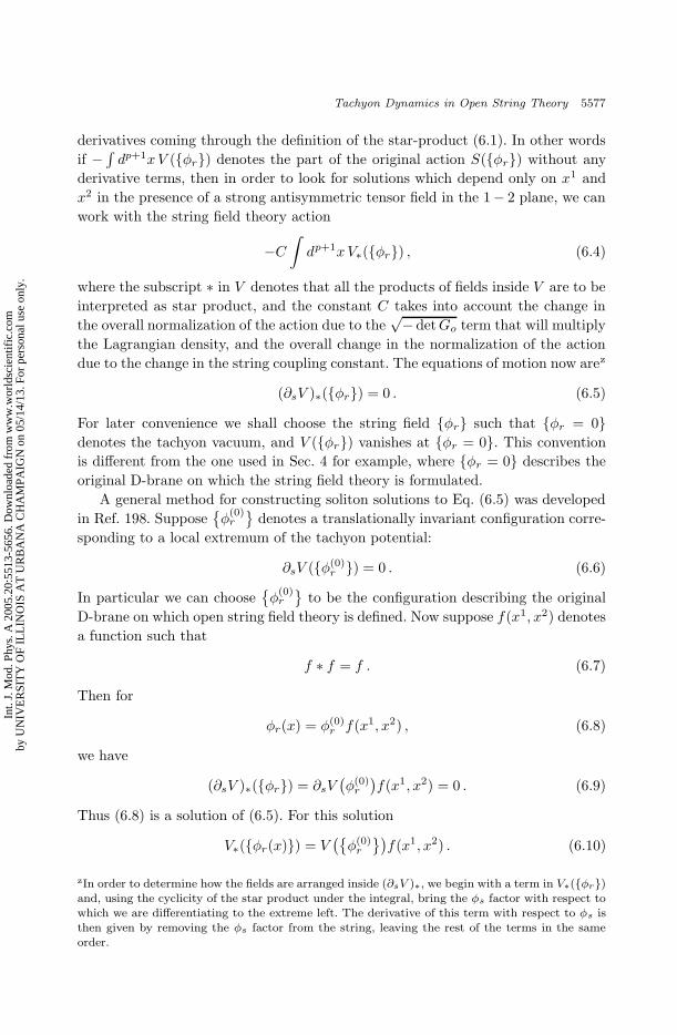
September 29, 2005 17:21 WSPC/139-IJMPA 02519
Tachyon Dynamics in Open String Theory 5577
derivatives coming through the definition of the star-product (6.1). In other words
if −∫
dp+1xV (φr) denotes the part of the original action S(φr) without any
derivative terms, then in order to look for solutions which depend only on x1 and
x2 in the presence of a strong antisymmetric tensor field in the 1− 2 plane, we can
work with the string field theory action
−C∫
dp+1xV∗(φr) , (6.4)
where the subscript ∗ in V denotes that all the products of fields inside V are to be
interpreted as star product, and the constant C takes into account the change in
the overall normalization of the action due to the√− detGo term that will multiply
the Lagrangian density, and the overall change in the normalization of the action
due to the change in the string coupling constant. The equations of motion now arez
(∂sV )∗(φr) = 0 . (6.5)
For later convenience we shall choose the string field φr such that φr = 0denotes the tachyon vacuum, and V (φr) vanishes at φr = 0. This convention
is different from the one used in Sec. 4 for example, where φr = 0 describes the
original D-brane on which the string field theory is formulated.
A general method for constructing soliton solutions to Eq. (6.5) was developed
in Ref. 198. Suppose
φ(0)r
denotes a translationally invariant configuration corre-
sponding to a local extremum of the tachyon potential:
∂sV (φ(0)r ) = 0 . (6.6)
In particular we can choose
φ(0)r
to be the configuration describing the original
D-brane on which open string field theory is defined. Now suppose f(x1, x2) denotes
a function such that
f ∗ f = f . (6.7)
Then for
φr(x) = φ(0)r f(x1, x2) , (6.8)
we have
(∂sV )∗(φr) = ∂sV(
φ(0)r
)
f(x1, x2) = 0 . (6.9)
Thus (6.8) is a solution of (6.5). For this solution
V∗(φr(x)) = V(
φ(0)r
)
f(x1, x2) . (6.10)
zIn order to determine how the fields are arranged inside (∂sV )∗, we begin with a term in V∗(φr)and, using the cyclicity of the star product under the integral, bring the φs factor with respect towhich we are differentiating to the extreme left. The derivative of this term with respect to φs isthen given by removing the φs factor from the string, leaving the rest of the terms in the sameorder.
Int.
J. M
od. P
hys.
A 2
005.
20:5
513-
5656
. Dow
nloa
ded
from
ww
w.w
orld
scie
ntif
ic.c
omby
UN
IVE
RSI
TY
OF
ILL
INO
IS A
T U
RB
AN
A C
HA
MPA
IGN
on
05/1
4/13
. For
per
sona
l use
onl
y.
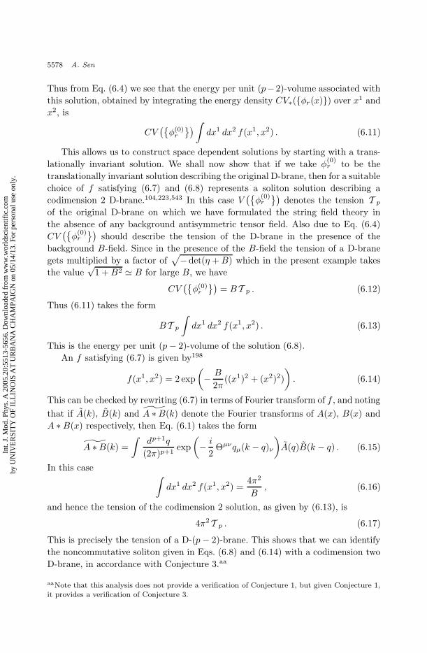
September 29, 2005 17:21 WSPC/139-IJMPA 02519
5578 A. Sen
Thus from Eq. (6.4) we see that the energy per unit (p−2)-volume associated with
this solution, obtained by integrating the energy density CV∗(φr(x)) over x1 and
x2, is
CV(
φ(0)r
)
∫
dx1 dx2 f(x1, x2) . (6.11)
This allows us to construct space dependent solutions by starting with a trans-
lationally invariant solution. We shall now show that if we take φ(0)r to be the
translationally invariant solution describing the original D-brane, then for a suitable
choice of f satisfying (6.7) and (6.8) represents a soliton solution describing a
codimension 2 D-brane.104,223,543 In this case V(
φ(0)r
)
denotes the tension T p
of the original D-brane on which we have formulated the string field theory in
the absence of any background antisymmetric tensor field. Also due to Eq. (6.4)
CV(
φ(0)r
)
should describe the tension of the D-brane in the presence of the
background B-field. Since in the presence of the B-field the tension of a D-brane
gets multiplied by a factor of√
− det(η +B) which in the present example takes
the value√
1 +B2 ' B for large B, we have
CV(
φ(0)r
)
= BT p . (6.12)
Thus (6.11) takes the form
BT p
∫
dx1 dx2 f(x1, x2) . (6.13)
This is the energy per unit (p− 2)-volume of the solution (6.8).
An f satisfying (6.7) is given by198
f(x1, x2) = 2 exp
(
− B
2π((x1)2 + (x2)2)
)
. (6.14)
This can be checked by rewriting (6.7) in terms of Fourier transform of f , and noting
that if A(k), B(k) and A ∗B(k) denote the Fourier transforms of A(x), B(x) and
A ∗B(x) respectively, then Eq. (6.1) takes the form
A ∗B(k) =
∫
dp+1q
(2π)p+1exp
(
− i
2Θµνqµ(k − q)ν
)
A(q)B(k − q) . (6.15)
In this case∫
dx1 dx2 f(x1, x2) =4π2
B, (6.16)
and hence the tension of the codimension 2 solution, as given by (6.13), is
4π2T p . (6.17)
This is precisely the tension of a D-(p− 2)-brane. This shows that we can identify
the noncommutative soliton given in Eqs. (6.8) and (6.14) with a codimension two
D-brane, in accordance with Conjecture 3.aa
aaNote that this analysis does not provide a verification of Conjecture 1, but given Conjecture 1,it provides a verification of Conjecture 3.
Int.
J. M
od. P
hys.
A 2
005.
20:5
513-
5656
. Dow
nloa
ded
from
ww
w.w
orld
scie
ntif
ic.c
omby
UN
IVE
RSI
TY
OF
ILL
INO
IS A
T U
RB
AN
A C
HA
MPA
IGN
on
05/1
4/13
. For
per
sona
l use
onl
y.
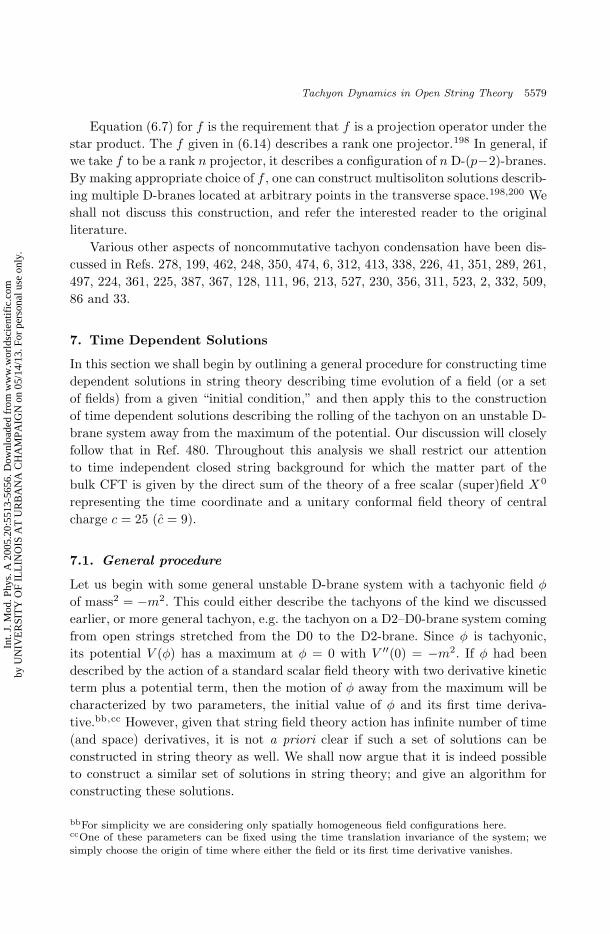
September 29, 2005 17:21 WSPC/139-IJMPA 02519
Tachyon Dynamics in Open String Theory 5579
Equation (6.7) for f is the requirement that f is a projection operator under the
star product. The f given in (6.14) describes a rank one projector.198 In general, if
we take f to be a rank n projector, it describes a configuration of n D-(p−2)-branes.
By making appropriate choice of f , one can construct multisoliton solutions describ-
ing multiple D-branes located at arbitrary points in the transverse space.198,200 We
shall not discuss this construction, and refer the interested reader to the original
literature.
Various other aspects of noncommutative tachyon condensation have been dis-
cussed in Refs. 278, 199, 462, 248, 350, 474, 6, 312, 413, 338, 226, 41, 351, 289, 261,
497, 224, 361, 225, 387, 367, 128, 111, 96, 213, 527, 230, 356, 311, 523, 2, 332, 509,
86 and 33.
7. Time Dependent Solutions
In this section we shall begin by outlining a general procedure for constructing time
dependent solutions in string theory describing time evolution of a field (or a set
of fields) from a given “initial condition,” and then apply this to the construction
of time dependent solutions describing the rolling of the tachyon on an unstable D-
brane system away from the maximum of the potential. Our discussion will closely
follow that in Ref. 480. Throughout this analysis we shall restrict our attention
to time independent closed string background for which the matter part of the
bulk CFT is given by the direct sum of the theory of a free scalar (super)field X0
representing the time coordinate and a unitary conformal field theory of central
charge c = 25 (c = 9).
7.1. General procedure
Let us begin with some general unstable D-brane system with a tachyonic field φ
of mass2 = −m2. This could either describe the tachyons of the kind we discussed
earlier, or more general tachyon, e.g. the tachyon on a D2–D0-brane system coming
from open strings stretched from the D0 to the D2-brane. Since φ is tachyonic,
its potential V (φ) has a maximum at φ = 0 with V ′′(0) = −m2. If φ had been
described by the action of a standard scalar field theory with two derivative kinetic
term plus a potential term, then the motion of φ away from the maximum will be
characterized by two parameters, the initial value of φ and its first time deriva-
tive.bb,cc However, given that string field theory action has infinite number of time
(and space) derivatives, it is not a priori clear if such a set of solutions can be
constructed in string theory as well. We shall now argue that it is indeed possible
to construct a similar set of solutions in string theory; and give an algorithm for
constructing these solutions.
bbFor simplicity we are considering only spatially homogeneous field configurations here.ccOne of these parameters can be fixed using the time translation invariance of the system; wesimply choose the origin of time where either the field or its first time derivative vanishes.
Int.
J. M
od. P
hys.
A 2
005.
20:5
513-
5656
. Dow
nloa
ded
from
ww
w.w
orld
scie
ntif
ic.c
omby
UN
IVE
RSI
TY
OF
ILL
INO
IS A
T U
RB
AN
A C
HA
MPA
IGN
on
05/1
4/13
. For
per
sona
l use
onl
y.
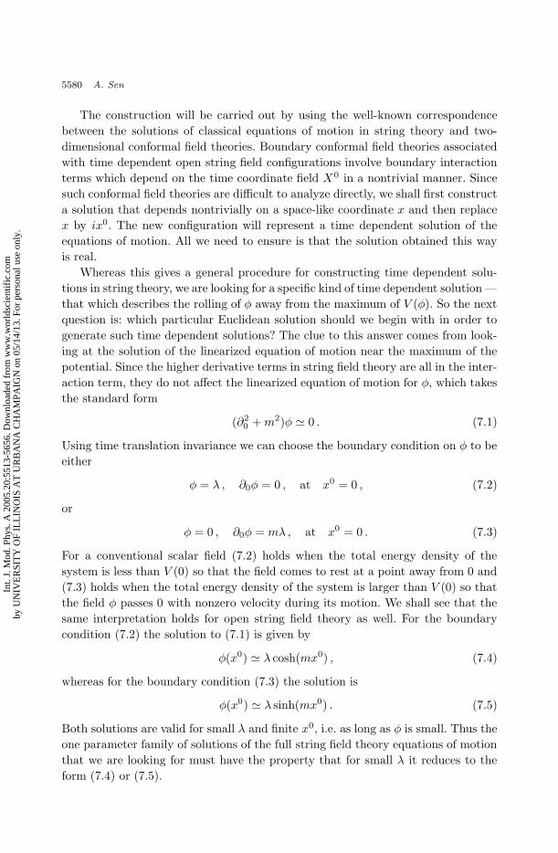
September 29, 2005 17:21 WSPC/139-IJMPA 02519
5580 A. Sen
The construction will be carried out by using the well-known correspondence
between the solutions of classical equations of motion in string theory and two-
dimensional conformal field theories. Boundary conformal field theories associated
with time dependent open string field configurations involve boundary interaction
terms which depend on the time coordinate field X0 in a nontrivial manner. Since
such conformal field theories are difficult to analyze directly, we shall first construct
a solution that depends nontrivially on a space-like coordinate x and then replace
x by ix0. The new configuration will represent a time dependent solution of the
equations of motion. All we need to ensure is that the solution obtained this way
is real.
Whereas this gives a general procedure for constructing time dependent solu-
tions in string theory, we are looking for a specific kind of time dependent solution —
that which describes the rolling of φ away from the maximum of V (φ). So the next
question is: which particular Euclidean solution should we begin with in order to
generate such time dependent solutions? The clue to this answer comes from look-
ing at the solution of the linearized equation of motion near the maximum of the
potential. Since the higher derivative terms in string field theory are all in the inter-
action term, they do not affect the linearized equation of motion for φ, which takes
the standard form
(∂20 +m2)φ ' 0 . (7.1)
Using time translation invariance we can choose the boundary condition on φ to be
either
φ = λ , ∂0φ = 0 , at x0 = 0 , (7.2)
or
φ = 0 , ∂0φ = mλ , at x0 = 0 . (7.3)
For a conventional scalar field (7.2) holds when the total energy density of the
system is less than V (0) so that the field comes to rest at a point away from 0 and
(7.3) holds when the total energy density of the system is larger than V (0) so that
the field φ passes 0 with nonzero velocity during its motion. We shall see that the
same interpretation holds for open string field theory as well. For the boundary
condition (7.2) the solution to (7.1) is given by
φ(x0) ' λ cosh(mx0) , (7.4)
whereas for the boundary condition (7.3) the solution is
φ(x0) ' λ sinh(mx0) . (7.5)
Both solutions are valid for small λ and finite x0, i.e. as long as φ is small. Thus the
one parameter family of solutions of the full string field theory equations of motion
that we are looking for must have the property that for small λ it reduces to the
form (7.4) or (7.5).
Int.
J. M
od. P
hys.
A 2
005.
20:5
513-
5656
. Dow
nloa
ded
from
ww
w.w
orld
scie
ntif
ic.c
omby
UN
IVE
RSI
TY
OF
ILL
INO
IS A
T U
RB
AN
A C
HA
MPA
IGN
on
05/1
4/13
. For
per
sona
l use
onl
y.
September 29, 2005 17:21 WSPC/139-IJMPA 02519
Tachyon Dynamics in Open String Theory 5581
For definiteness we shall from now on concentrate on the class of solutions with
total energy density less than V (0), but the analysis can be easily generalized to the
other case.dd We now note that (7.4) can be obtained from the Euclidean solution
φ(x) ' λ cos(mx) , (7.6)
under the replacement x→ ix0. Thus we need to search for a one parameter family
of Euclidean solutions which for small value of the parameter λ, reduces to (7.6).
Given such a one parameter family of solutions, we can construct one parameter
family of time dependent solutions by the replacement x→ ix0.ee
To proceed further, we shall, for definiteness, concentrate on the bosonic string
theory, although the analysis can be easily generalized to the superstring theory.
Since the tachyon has mass2 = −m2, the zero momentum tachyon vertex operator
Vφ must have dimension (1−m2) so that Vφeik·X has dimension 1 for k2 = m2. For
small λ, switching on the background (7.6) corresponds to deforming the original
boundary CFT by a boundary perturbation of the form
λ
∫
dt Vφ(t) cos(mX(t)) , (7.7)
where t denotes a parameter labeling the boundary of the worldsheet. Since
Vφ cos(mX) has conformal dimension 1, the deformed theory represents a con-
formal field theory to first order in λ. In order to construct a one parameter family
of solutions of the string field theory equations of motion, we need to construct a
family of conformal field theories labeled by λ, which to first order in λ agrees with
the deformed theory (7.7).
In special cases, Vφ cos(mX) may represent an exactly marginal operator in
string field theory, in which case (7.7) represents a conformal field theory even for
finite λ, and our task is over. However even in this case, for finite λ the parameter
λ appearing in (7.7) may not agree exactly with the value of T at x0 = 0 (which
in turn depends on the precise definition of the tachyon field, and varies between
different formulations of string field theory for example.) Thus it is more appropriate
to label the perturbation as
λ
∫
dt Vφ(t) cos(mX(t)) , (7.8)
with λ = λ+ O(λ2).
In the generic case Vφ cos(mX) is not an exactly marginal operator since its β-
function βλ will have contribution of order λ3 and higher.ff In this case we proceed
ddIn fact the solution of type (7.5) can be obtained from those of type (7.4) by the formal replace-ment x0 → x0 − iπ/2m, λ → iλ.eeThe original idea of constructing time dependent solution in open string theory by Wick rotatingEuclidean solution is due to Ref. 215.ffNote that due to X → X +π/m, λ → −λ symmetry of the deformation, β
λreceives contribution
only to odd orders in λ.
Int.
J. M
od. P
hys.
A 2
005.
20:5
513-
5656
. Dow
nloa
ded
from
ww
w.w
orld
scie
ntif
ic.c
omby
UN
IVE
RSI
TY
OF
ILL
INO
IS A
T U
RB
AN
A C
HA
MPA
IGN
on
05/1
4/13
. For
per
sona
l use
onl
y.

September 29, 2005 17:21 WSPC/139-IJMPA 02519
5582 A. Sen
as follows. Instead of considering the deformation (7.8), we consider deformation
by the operator
λ
∫
dt Vφ(t) cos(ωX(t)) , (7.9)
where ω is a constant that will be fixed shortly. Since the perturbing operator has
dimension (ω2 − m2 + 1), βλ now receives contribution linear in λ, and the full
β-function is given by
βλ = (ω2 −m2)λ+ g(ω, λ) , (7.10)
where g(ω, λ) denotes higher order contribution to the β-function. We now adjust
ω so that the right-hand side of (7.10) vanishes. Since g(ω, λ) ∼ λ3, we can get a
solution of the form
ω = m+ O(λ2) . (7.11)
This gives a way to generate a one parameter family of boundary CFT’s labeled
by λ, which for small λ corresponds to the solution (7.6) with λ ' λ. Given this
conformal field theory, we can calculate the energy–momentum tensor and sources
of other massless fields like the dilaton, antisymmetric tensor field etc. from the
boundary state associated with this BCFT. (If the deformed boundary CFT is
solvable then we can find an exact expression for the boundary state as in Sub-
sec. 3.3; otherwise we may need to compute it as a perturbation series in λ.)
Note that in the above analysis we have not included the β-functions for any
operator other than the original perturbing operator. In order to get a conformal
field theory we need to ensure that the β-function for every other operator also
vanishes. What we have done here is to implicitly assume that the other operators
have been “integrated out” (in a space–time sense) so that we can talk in terms of
the “effective” β-function of this single operator Vφ cos(ωX). To see explicitly what
this means let Oi denote a complete set of boundary operators in the theory
other than Vφ cos(ωX), and let hi be the conformal weight of Oi. We add to the
action the boundary term
∑
i
gi
∫
dtOi(t) , (7.12)
besides (7.9). Then the β-function βi of gi and βλ have the form
βi = (hi − 1)gi + Fi(ω, ~g, λ) , βλ = (ω2 −m2)λ+ F (ω, ~g, λ) . (7.13)
Fi and F contains terms quadratic and higher order in gi and λ. From this we
see that as long as hi 6= 1, we can solve for the gi’s and (ω −m) in power series
in λ beginning at quadratic or higher order. In particular we can first solve the
βi = 0 equations to express each gi as a function of λ, and substitute this back
into the expression for βλ to get an equation of the form (7.10). This procedure of
Int.
J. M
od. P
hys.
A 2
005.
20:5
513-
5656
. Dow
nloa
ded
from
ww
w.w
orld
scie
ntif
ic.c
omby
UN
IVE
RSI
TY
OF
ILL
INO
IS A
T U
RB
AN
A C
HA
MPA
IGN
on
05/1
4/13
. For
per
sona
l use
onl
y.
September 29, 2005 17:21 WSPC/139-IJMPA 02519
Tachyon Dynamics in Open String Theory 5583
“integrating out” the other operators breaks down if there are operators of dimen-
sion ' 1 other than Vφ cos(ωX) since in this case we can no longer solve the βi = 0
equations to express gi as a power series in λ. This difficulty is of course a reflection
of the well-known difficulty in integrating out the massless fields.
In particular we can consider operators ∂X or Vφ sin(ωX) both of which will
have dimension ' 1. Fortunately both these operators are odd under X → −X ,
and hence are not generated in the operator product of Vφ cos(ωX) with itself, since
the latter operator is even under X → −X . In the generic case we do not expect
any other dimension ' 1 operator to appear in the operator product of Vφ cos(ωX)
with itself, but there may be special cases where such operators do appear.gg
In order to generate the time dependent solution, we now make the replace-
ment X → iX0. This corresponds to deforming the original boundary CFT by the
operator
λ
∫
dt Vφ(t) cosh(ωX0(t)) . (7.14)
ω is determined in terms of λ by the same equation as in the Euclidean case.hh
The corresponding energy–momentum tensor and sources of other massless fields
are also obtained by the making the replacement x → ix0 in the corresponding
expressions in the Euclidean theory.
This illustrates the general method for constructing a one parameter family of
solutions labeled by λ which reduce to (7.4) for small λ. In order to generate another
one parameter family of BCFT labeled by λ which reduce to (7.5) for small λ, we
simply make a replacement X0 → X0 − i π2ω , λ→ iλ in the solution derived above.
This corresponds to deforming the original BCFT by the operator
λ
∫
dt Vφ(t) sinh(ωX0(t)) , (7.15)
and hence corresponds to a solution of the form (7.5) for small λ since ω → m as
λ → 0.
It is clear that the same method can be used to construct time dependent
solutions describing rolling of tachyons on unstable D-brane systems in superstring
theory as well. The method can also be generalized to describe simultaneous rolling
of multiple tachyons.480
ggIn fact the general method outlined here also holds for generating time dependent solutionsin closed string theory, but the dimension (1, 1) operators associated with the zero momentumgraviton/dilaton vertex operators cause obstruction to this procedure. It may be possible to avoidthis problem in case of localized tachyons,3 since in this case the rolling tachyon generates alocalized source for the bulk graviton/dilaton field, and hence we can solve the equations ofmotion of these massless fields in the presence of these localized sources in order to get a consistentconformal field theory.hhIf we are using the picture in which the higher modes have not been integrated out, then wealso need to add perturbations generated by the Wick rotated version of (7.12). These picturesdiffer from each other by a choice of renormalization scheme for the worldsheet field theory.
Int.
J. M
od. P
hys.
A 2
005.
20:5
513-
5656
. Dow
nloa
ded
from
ww
w.w
orld
scie
ntif
ic.c
omby
UN
IVE
RSI
TY
OF
ILL
INO
IS A
T U
RB
AN
A C
HA
MPA
IGN
on
05/1
4/13
. For
per
sona
l use
onl
y.
September 29, 2005 17:21 WSPC/139-IJMPA 02519
5584 A. Sen
7.2. Specific applications
We shall now apply the general method discussed in the last section to describe
the rolling of spatially homogeneous tachyon field configuration on a Dp-brane of
bosonic string theory lying along x0, x26−p, . . . , x25.477,478 In this case the vertex
operator Vφ of the zero momentum tachyon is just the identity operator, and the
tachyon has mass2 = −1. As a result, to lowest order in λ, the analog of the
perturbation (7.8) in the Euclidean theory is given by
λ
∫
dt cos(X(t)) . (7.16)
This is identical to the perturbation (3.8) with λ identified to −α and represents an
exactly marginal deformation of the original BCFT.ii As a result, the deformation
(7.16) represents a BCFT for finite λ as well. Put another way, in this case Eq. (7.11)
is replaced by
ω = m = 1 , (7.17)
for all λ.
Making the replacement X → iX0 we see that the rolling tachyon solution is
given by perturbing the original BCFT by the operator
λ
∫
dt cosh(X0(t)) . (7.18)
The energy–momentum tensor Tµν and the dilaton charge density Q associated with
this solution can be obtained by making the replacement X → iX0, X0 → −iX25,
α → −λ in (3.46)–(3.48). This gives
Q = T pf(x0)δ(x⊥) , T00 = T p cos2(πλ)δ(x⊥) ,
TMN = −T pf(x0)δMNδ(x⊥) for (26 − p) ≤M, N ≤ 25 ,(7.19)
with all other components of Tµν being zero. Here
f(x0) = f(ix0)|α=−λ =1
1 + ex0 sin(λπ)+
1
1 + e−x0 sin(λπ)− 1 . (7.20)
This reproduces (2.22)–(2.24) and (2.30) after taking into account the fact that the
results in Sec. 2 were quoted for a Dp-brane lying along x0, x1, . . . , xp, whereas the
results obtained here are for Dp-branes lying along x0, x26−p, . . . , x25.
As discussed in the previous subsection, the other one parameter family of solu-
tions, valid when the total energy carried by the tachyon field configuration is
larger than the tension of the D-brane, is obtained by making the replacement
x0 → x0 − iπ/2, λ → iλ. Making these replacements in (7.19) and (7.20) gives
iiIn the analysis of the perturbation (3.8) we took X to be compact whereas here X, being relatedby Wick rotation to the time coordinate X0, is noncompact. However the marginality of theoperator does not depend on whether X is compact or not.
Int.
J. M
od. P
hys.
A 2
005.
20:5
513-
5656
. Dow
nloa
ded
from
ww
w.w
orld
scie
ntif
ic.c
omby
UN
IVE
RSI
TY
OF
ILL
INO
IS A
T U
RB
AN
A C
HA
MPA
IGN
on
05/1
4/13
. For
per
sona
l use
onl
y.
September 29, 2005 17:21 WSPC/139-IJMPA 02519
Tachyon Dynamics in Open String Theory 5585
the nonzero components of the energy–momentum tensor and the dilaton charge
density Q(x) to be
Q = T pf(x0)δ(x⊥) , T00 = T p cosh2(πλ)δ(x⊥) ,
TMN = −T pf(x0)δMNδ(x⊥) for (26 − p) ≤M, N ≤ 25 ,(7.21)
where
f(x0) =1
1 + ex0 sinh(λπ)+
1
1 − e−x0 sinh(λπ)− 1 . (7.22)
This reproduces (2.22), (2.27), (2.28) and (2.30).
The analysis in the case of Dp–Dp-brane pair in superstring theory proceeds in
an identical manner. If the total energy per unit p-volume is less than Ep where
Ep is the tension of the original brane system, we need to switch on a tachyon
backgroundjj
T =√
2λ cosh(X0/√
2) . (7.23)
This is related to the background (3.17) for R = 1√2
by the replacement
x → ix0 + π/√
2 , α→ λ , (7.24)
and hence represents an exactly marginal deformation of the theory. Making these
replacements in (3.51)–(3.53), we get the nonzero components of Tµν and the dilaton
charge density Q to be
T00 = Ep cos2(πλ)δ(x⊥) ,
TMN = −Epf(x0)δMNδ(x⊥) for (10 − p) ≤M, N ≤ 9 ,
Q(x) = Epf(x0)δ(x⊥) ,
(7.25)
f(x0) =1
1 + e√
2x0 sin2(λπ)+
1
1 + e−√
2x0 sin2(λπ)− 1 . (7.26)
This reproduces (2.12)–(2.14) and (2.17) after taking into account the fact that the
results of Sec. 2 were quoted for a brane–antibrane system along x0, . . . , xp whereas
here the original brane–antibrane system is taken to be along x0, x10−p, . . . , x9.
For total energy > Ep we need to switch on a tachyon background
T =√
2λ sinh(X0/√
2) . (7.27)
This is related to (7.23) by the replacement x0 → x0 − iπ/√
2, λ → iλ. Making
these replacements in (7.25), (7.26) gives
T00 = Ep cosh2(πλ)δ(x⊥) ,
TMN = −Epf(x0)δMNδ(x⊥) for (10− p) ≤M, N ≤ 9 ,
Q(x) = Epf(x0)δ(x⊥) ,
(7.28)
jjThe√
2 multiplying λ is part of the normalization convention for λ.
Int.
J. M
od. P
hys.
A 2
005.
20:5
513-
5656
. Dow
nloa
ded
from
ww
w.w
orld
scie
ntif
ic.c
omby
UN
IVE
RSI
TY
OF
ILL
INO
IS A
T U
RB
AN
A C
HA
MPA
IGN
on
05/1
4/13
. For
per
sona
l use
onl
y.
September 29, 2005 17:21 WSPC/139-IJMPA 02519
5586 A. Sen
with
f(x0) =1
1 + e√
2x0 sinh2(λπ)+
1
1 + e−√
2x0 sinh2(λπ)− 1 . (7.29)
All other components of Tµν vanish. This reproduces (2.15)–(2.17).
Similar method can be used for getting the corresponding results for the non-
BPS D-brane. In fact since a non-BPS D-brane is obtained by modding out a brane–
antibrane system by (−1)FL , and since Tµν is invariant under this transformation,
the results for the sources for NS–NS sector fields produced by non-BPS D-brane
are identical to those on a D–D pair except for a change in the overall normalization.
Information about the sources for the RR fields associated with the rolling tachyon
background on a non-BPS D-brane, as given in Eqs. (2.18), can be obtained from
Eq. (3.54) by the replacement (7.24). Equation (2.19) may be obtained from (2.18)
by the replacement x0 → x0 − iπ/√
2, λ → iλ.
The boundary state can also be used to determine the source terms for massive
closed string states. For this we need to find the complete boundary state in the
Euclidean theory and replace X by iX0. We shall illustrate this in the context
of bosonic string theory, but in principle the same procedure works for superstring
theory. The |B〉c=25 and |B〉ghost parts of the boundary state are given by Eqs. (3.36)
and (3.37) respectively. Thus the nontrivial part is |B〉c=1. The complete expression
for |B〉c=1 for a general deformation parameter λ can be obtained by following the
procedure outlined in Subsec. 3.3.79,445,kk In order to describe the results we need
to review a few facts about the spectrum of the c = 1 conformal field theory
described by a single noncompact scalar field X . This theory contains a set of
Virasoro primary states labeled by SU(2) quantum numbers (j,m) and have the
form124,ll
|j,m〉 = Pj,me2imX(0)|0〉 , (7.30)
where Pj,m is some combination of the X oscillators of level (j2 −m2, j2 −m2).
Thus |j,m〉 carriesX-momentum 2m and (L0, L0) eigenvalue (j2, j2). For any given
primary state |j,m〉 we have an associated Virasoro Ishibashi state257 |j,m〉〉, defined
as the unique linear combination of the primary |j,m〉 and all Virasoro descendants
of |j,m〉 such that Ln − L−n annihilate the state for every n. We shall normalize
kkThe analysis of Subsec. 3.3 was carried out for compact X. The result for noncompact X isobtained by simply dropping from the result of Subsec. 3.3 all terms in the boundary state carryingnonzero winding number.llThe underlying SU(2) group is inherited from the theory with X-coordinate compactified on acircle of radius 1. Although SU(2) is not a symmetry of the theory when X is noncompact, itis still useful to classify states with integer X-momentum. In fact the theory with compact Xactually has an SU(2)L × SU(2)R symmetry and the theory with noncompact X contains a moregeneral set of primary states carrying left and right SU(2) quantum numbers (j,m) and (j ′,m)respectively. The states with j 6= j′ will not be important for our discussion.
Int.
J. M
od. P
hys.
A 2
005.
20:5
513-
5656
. Dow
nloa
ded
from
ww
w.w
orld
scie
ntif
ic.c
omby
UN
IVE
RSI
TY
OF
ILL
INO
IS A
T U
RB
AN
A C
HA
MPA
IGN
on
05/1
4/13
. For
per
sona
l use
onl
y.
September 29, 2005 17:21 WSPC/139-IJMPA 02519
Tachyon Dynamics in Open String Theory 5587
the Ishibashi states so that when we express exp(
∑∞n=1
1nα−nα−n
)
e2imX(0)|0〉 as
a linear combination of the Ishibashi states built on various primaries, the state
|j,m〉〉 appears with coefficient 1 for every j ≥ |m|:mm
exp
( ∞∑
n=1
1
nα−nα−n
)
e2imX(0)|0〉 =∑
j≥|m||j,m〉〉 . (7.31)
For the deformation (7.16) |B〉c=1 may be expressed in terms of these Ishibashi
states as79,445,488
|B〉c=1 = exp
( ∞∑
n=1
1
nα−nα−n
)
f(X(0))|0〉 + |B〉c=1 , (7.32)
where
f(x) =1
1 + sin(πλ)eix+
1
1 + sin(πλ)e−ix− 1 , (7.33)
|B〉c=1 =∑
j≥1
j−1∑
m=−j+1
fj,m(λ)|j,m〉〉 , (7.34)
fj,m(λ) = Djm,−m(2πλ)
(−1)2m
Djm,−m(π)
− (−1)2m sin2|m|(πλ) . (7.35)
Djm,m′(θ) are the representation matrices of the SU(2) group element eiθσ1/2 in the
spin j representation.
If |B〉c=1 denotes the continuation of |B〉c=1 to the Minkowski space, then the
complete boundary state |B〉 in the Minkowski space may be expressed as
|B〉 = |B1〉 + |B2〉 , (7.36)
where
|B1〉 = T p exp
(
−∞∑
n=1
1
nα0−nα
0−n
)
f(X0(0))|0〉
⊗∫
d25−pk⊥(2π)25−p
exp
( ∞∑
n=1
25∑
s=1
(−1)ds1
nαs−nα
s−n
)
|~k‖ = 0, ~k⊥〉
⊗ exp
(
−∞∑
n=1
(b−nc−n + b−nc−n)
)
(c0 + c0)c1c1|0〉 , (7.37)
mmIn this convention, the usual δ-function normalized primary state |j,m〉 appears in |j,m〉〉 withunit coefficient.490
Int.
J. M
od. P
hys.
A 2
005.
20:5
513-
5656
. Dow
nloa
ded
from
ww
w.w
orld
scie
ntif
ic.c
omby
UN
IVE
RSI
TY
OF
ILL
INO
IS A
T U
RB
AN
A C
HA
MPA
IGN
on
05/1
4/13
. For
per
sona
l use
onl
y.
September 29, 2005 17:21 WSPC/139-IJMPA 02519
5588 A. Sen
and
|B2〉 = T p|B〉c=1 ⊗∫
d25−pk⊥(2π)25−p
exp
( ∞∑
n=1
25∑
s=1
(−1)ds1
nαs−nα
s−n
)
|~k‖ = 0, ~k⊥〉
⊗ exp
(
−∞∑
n=1
(b−nc−n + b−nc−n)
)
(c0 + c0)c1c1|0〉 . (7.38)
ds is an integer which is zero for Dirichlet directions and one for Neumann directions.
f(x0) = f(ix0) is given in (7.20).
|B1〉 produces source terms proportional to f(x0) for various closed string fields,
and hence these sources fall off to zero as x0 → ±∞. On the other hand since |B〉c=1
is a linear combination of Virasoro descendants over higher level primaries, and since
these primaries occur at discrete values of momenta, these terms cannot be reorga-
nized by summing over momenta as in Eq. (3.46). Thus its Minkowski version |B〉c=1
will involve linear combinations of Virasoro descendants of exp(
±nX0(0))
|0〉 for
integer n and |B2〉, which contains |B〉c=1, will have source terms for various higher
level closed string fields which grow exponentially.412,94,418 Thus |B2〉 has the form
|B2〉 = T p
∞∑
n=−∞
∞∑
N=1
∫
d25−pk⊥(2π)25−p
O(n)N (c0 + c0)c1c1e
nX0(0)|k0 = 0, ~k‖ = 0, ~k⊥〉 ,
(7.39)
where O(n)N is some fixed combination of negative moded oscillators of total level
(N,N). We shall return to a discussion of these terms in Secs. 10 and 11.
An interesting limit to consider is the λ→ 12 limit. As pointed out in Eq. (2.25),
in this limit f(x0) vanishes, and hence |B1〉 vanishes. It is also easy to see using
(7.35) that fj,m(1/2) = 0. Thus in the λ→ 12 limit |B〉c=1, its analytic continuation
|B〉c=1 and hence |B2〉 vanishes. This shows that at λ = 12 not only the sources for
the massless closed string fields vanish, but the sources for all the massive closed
string fields also vanish. This is consistent with the identification of the λ = 12 point
as the vacuum without any D-brane.
It is easy to verify that |B1〉 is BRST invariant, i.e.
(QB + QB)|B1〉 = 0 . (7.40)
Indeed we have the stronger relation
(QB + QB)
[
exp
(
−∞∑
n=1
1
nα0−nα
0−n
)
|k0〉
⊗ exp
( ∞∑
n=1
25∑
s=1
(−1)ds1
nαs−nα
s−n
)
|~k‖ = 0, ~k⊥〉
⊗ exp
(
−∞∑
n=1
(b−nc−n + b−nc−n)
)
(c0 + c0)c1c1|0〉]
= 0 , (7.41)
Int.
J. M
od. P
hys.
A 2
005.
20:5
513-
5656
. Dow
nloa
ded
from
ww
w.w
orld
scie
ntif
ic.c
omby
UN
IVE
RSI
TY
OF
ILL
INO
IS A
T U
RB
AN
A C
HA
MPA
IGN
on
05/1
4/13
. For
per
sona
l use
onl
y.
September 29, 2005 17:21 WSPC/139-IJMPA 02519
Tachyon Dynamics in Open String Theory 5589
for any k0 and ~k⊥. Thus (QB + QB)|B1〉, which may be expressed as a linear
combination of the states appearing on the left-hand side of (7.41), also vanishes.
Since |B〉 = |B1〉 + |B2〉 is BRST invariant, this shows that |B2〉 is also BRST
invariant:
(QB + QB)|B2〉 = 0 . (7.42)
From (7.41) it follows that |B1〉 given in (7.37) is BRST invariant for any choice
of the function f(x0). Thus the BRST invariance of |B1〉 does not impose any
condition on the time dependence f(x0) of this boundary state. In contrast the
time dependence of the boundary state |B2〉 is fixed by the requirement of BRST
invariance488,490 since in the c = 1 conformal field theory the primary states |j,m〉for |m| < j exist only for integer X-momentum 2m. This suggests that the coef-
ficients of |j,m〉〉 appearing in |B2〉 can be thought of as conserved charges.488,30
We shall discuss this point in detail in the context of two-dimensional string theory
in Sec. 11 where we shall also identify these charges with appropriate conserved
charges in the matrix model description of the theory.
Before we conclude this section we note that in principle we should be able to
study the time dependent solutions described here in string field theory by starting
with the Euclidean solution describing the lump or a kink on a circle of appropriate
radius (1 for bosonic string theory and 1√2
for superstring) and then making an
inverse Wick rotation.379,160,24 So far however this has not yielded any useful insight
into the structure of these solutions. Various other approaches to studying these
time dependent solutions in string field theory have been discussed in Refs. 299,
500, 349, 458, 153, 141 and 142.
Other aspects of time dependent classical solutions describing rolling of the
tachyon away from the maximum of the potential have been discussed in Refs. 502,
236, 148, 458, 153 and 87.
8. Effective Action Around the Tachyon Vacuum
A question that arises naturally out of the studies in the previous sections is:
is it possible to describe the physics around the tachyon vacuum by a low energy
effective action? Given that the tachyon field near the top of the potential has a
mass2 of the order of the string scale, one would not naively expect any such action
to exist. Furthermore, since around the tachyon vacuum we do not expect to get
any physical open string states, there is no S-matrix with which we could com-
pare the predictions of the effective action. Thus it would seem that not only is it
unlikely that we have a low energy effective action describing the physics around
the tachyon vacuum, but that the very question does not make sense due to the
absence of physical states around such a vacuum.
We should keep in mind however that in string theory there is another way of
checking the correctness of the classical effective action — namely by demanding
Int.
J. M
od. P
hys.
A 2
005.
20:5
513-
5656
. Dow
nloa
ded
from
ww
w.w
orld
scie
ntif
ic.c
omby
UN
IVE
RSI
TY
OF
ILL
INO
IS A
T U
RB
AN
A C
HA
MPA
IGN
on
05/1
4/13
. For
per
sona
l use
onl
y.
September 29, 2005 17:21 WSPC/139-IJMPA 02519
5590 A. Sen
that the solutions of the classical equations of motion derived from this effective
action should correspond to appropriate conformal field theories. In particular for
open string theory the classical solutions should be in one-to-one correspondence
with conformally invariant boundary deformations of the worldsheet theory. As we
saw in Sec. 7, there are families of known time dependent solutions around the
tachyon vacuum labeled by the parameter λ, and we could ask if it is possible
to construct an effective action that reproduces these solutions. Also the effective
action must have the property that perturbative quantization of the theory based
on this action should fail to give rise to any physical particle like states. We shall
show that it is indeed possible to construct an effective action satisfying these
criteria at a qualitative level. However we shall not be able to derive this effective
action from first principles, e.g. by comparison with any S-matrix elements, or make
any definitive statement about the region of validity of this effective action. Some
attempts to partially justify the validity of this effective action has been made in
Refs. 319 and 398.
8.1. Effective action involving the tachyon
We begin with the purely tachyonic part of the action, ignoring the massless fields
on the D-brane worldvolume. In this case the proposed action around the tachyon
vacuum is given by174,273,52,479,175–178,496,295
S =
∫
dp+1xL ,
L = −V (T )√
1 + ηµν∂µT∂νT
= −V (T )√− detA ,
(8.1)
where
Aµν = ηµν + ∂µT∂νT . (8.2)
The potential V (T ) has a maximum at T = 0 and has the asymptotic form
V (T ) ' e−αT/2 for large T , (8.3)
with
α = 1 for bosonic string theory
=√
2 for superstring theory . (8.4)
In this parametrization the potential has a minimum at infinity. The energy–
momentum tensor can be computed from the action (8.1) by first minimally
Int.
J. M
od. P
hys.
A 2
005.
20:5
513-
5656
. Dow
nloa
ded
from
ww
w.w
orld
scie
ntif
ic.c
omby
UN
IVE
RSI
TY
OF
ILL
INO
IS A
T U
RB
AN
A C
HA
MPA
IGN
on
05/1
4/13
. For
per
sona
l use
onl
y.
September 29, 2005 17:21 WSPC/139-IJMPA 02519
Tachyon Dynamics in Open String Theory 5591
coupling it to a background metric, and then calculating the functional derivative
of the action with respect to the background metric. The result is given bynn
Tµν =V (T )∂µT∂νT
√
1 + ηρσ∂σT∂ρT− V (T )ηµν
√
1 + ηρσ∂ρT∂σT . (8.5)
We shall first verify that the action (8.1) produces the correct large x0 behavior
of the pressure for spatially homogeneous, time dependent field configurations. For
such configurations the conserved energy density is given by
T00 = V (T )(1− (∂0T )2)−1/2 . (8.6)
Since T00 is conserved, and V (T ) → 0 for large T , we see that for any given T00, as
T → ∞, ∂0T → 1 and hence T → x0 + constant. In particular using (8.3) we can
show that for large x0 the solution has the form
T = x0 + Ce−αx0
+ O(e−2αx0
) , (8.7)
after shifting the origin of x0 so as to remove the additive constant that might
otherwise appear in the expression for T . One way to check that (8.7) gives the
correct form of the solution is to note that the leading contribution to T00 computed
from this configuration remains constant in time:
T00 ' 1√2αC
. (8.8)
The pressure associated with this configuration is given by
p = T11 = −V (T )(1 − (∂0T )2)1/2 ' −√
2αCe−αx0
. (8.9)
Using the choice of α given in Eq. (8.4) one can see that (8.9) is in precise agreement
with the asymptotic forms of (2.24) and (2.28) for the bosonic string or (2.14)
and (2.16) for the superstring for large x0. In particular the pressure vanishes
asymptotically.
Given the success of the effective action in reproducing the asymptotic form of
Tµν , it is natural to ask if it can also reproduce the sources for the dilaton and the
RR fields associated with the rolling tachyon solution on an unstable D-brane. For
this we need to know how the dilaton ΦD and the RR p-form fields C(p) couple to
this effective field theory. For a non-BPS D-brane of type II string theory, following
coupling to ΦD , C(p) and the string metric Gµν seems to reproduce qualitatively
the dilaton and RR source terms and Tµν associated with a rolling tachyon solution:
S = −∫
dp+1x e−ΦDV (T )√− detA +
∫
W (T )dT ∧ C(p) , (8.10)
Aµν = Gµν + ∂µT∂νT , (8.11)
nnIn writing down the expression for the energy–momentum tensor, it will be understood thatthese are localized on the plane of the brane by a position space delta function in the transversecoordinates. Also only the components of the energy–momentum tensor along the worldvolume ofthe brane are nonzero.
Int.
J. M
od. P
hys.
A 2
005.
20:5
513-
5656
. Dow
nloa
ded
from
ww
w.w
orld
scie
ntif
ic.c
omby
UN
IVE
RSI
TY
OF
ILL
INO
IS A
T U
RB
AN
A C
HA
MPA
IGN
on
05/1
4/13
. For
per
sona
l use
onl
y.
September 29, 2005 17:21 WSPC/139-IJMPA 02519
5592 A. Sen
where W (T ) is some even function of T which goes to zero asymptotically as
e−T/√
2.541,251,469,479 The sources for Gµν , ΦD and C(p) can be calculated by vary-
ing this action with respect to these closed string fields and then setting Gµν = ηµν ,
ΦD = 0, C(p) = 0. The source for Gµν gives us back the Tµν given in (8.5) whereas
the sources for ΦD and C(p), evaluated for the asymptotic solution (8.7) reproduces
the asymptotic form of the exact stringy answers (2.17)–(2.19). For a D-p-brane in
bosonic string theory and a D–D system of type II string theory the coupling to
the Ramond–Ramond field C(p) is absent from (8.10), but the dilaton coupling has
the same form.
8.2. Classical solutions around the tachyon vacuum
Next we shall demonstrate the absence of perturbative states upon quantization of
the theory around the tachyon vacuum. Since a priori it is not clear how to quantize
a nonlinear theory of this type, we shall use a pragmatic definition of the absence
of perturbative states. Since in conventional field theory perturbative states are
associated with plane wave solutions, we shall assume that absence of perturbative
quantum states implies absence of plane-wave solutions (which are not pure gauge)
and vice versa. Thus we need to show the absence of plane-wave solutions around
the tachyon vacuum in this theory.
This leads us to the analysis of classical solutions in this theory. Since around the
tachyon vacuum V (T ) = 0 and hence the action (8.1) vanishes, it is more convenient
to work in the Hamiltonian formalism.188,548,341,214,342,476,343,479,189 Defining the
momentum conjugate to T as
Π(x) =δS
δ(∂0T (x))=
V (T )∂0T√
1 − (∂0T )2 + ( ~∇T )2, (8.12)
we can construct the Hamiltonian H
H =
∫
dpx(Π∂0T −L) ≡∫
dpxH ,
H = T00 =√
Π2 + (V (T ))2√
1 + ( ~∇T )2 .
(8.13)
The equations of motion derived from this Hamiltonian take the form
∂0Π(x) = − δH
δT (x)= ∂j
(
√
Π2 + V 2∂jT
√
1 + ( ~∇T )2
)
− V (T )V ′(T )√Π2 + V 2
√
1 + ( ~∇T )2 , (8.14)
∂0T (x) =δH
δΠ(x)=
Π√Π2 + V 2
√
1 + ( ~∇T )2 . (8.15)
Int.
J. M
od. P
hys.
A 2
005.
20:5
513-
5656
. Dow
nloa
ded
from
ww
w.w
orld
scie
ntif
ic.c
omby
UN
IVE
RSI
TY
OF
ILL
INO
IS A
T U
RB
AN
A C
HA
MPA
IGN
on
05/1
4/13
. For
per
sona
l use
onl
y.
September 29, 2005 17:21 WSPC/139-IJMPA 02519
Tachyon Dynamics in Open String Theory 5593
In the limit of large T (i.e. near the tachyon vacuum) at fixed Π, we can ignore the
V 2 ' e−αT term, and the Hamiltonian and the equations of motion take the form
H =
∫
dpx|Π|√
1 + ( ~∇T )2 , (8.16)
∂0Π(x) = ∂j
(
|Π| ∂jT√
1 + ( ~∇T )2
)
, (8.17)
∂0T (x) =Π
|Π|
√
1 + ( ~∇T )2 . (8.18)
From (8.18), we see that in this limit we have (∂0T )2 − ( ~∇T )2 = 1.
These equations can be rewritten in a suggestive form by defining479
uµ ≡ −∂µT , ε(x) ≡ |Π(x)|/
√
1 + ( ~∇T )2 . (8.19)
Equations (8.17) and (8.18) then take the form
ηµνuµuν = −1 , ∂µ(ε(x)uµ) = 0 . (8.20)
Expressed in terms of these new variables, Tµν given in (8.5) take the form
Tµν = ε(x)uµuν , (8.21)
where we have used Eq. (8.15) and the small V (T ) approximation. We now note that
(8.20) and (8.21) are precisely the equations governing the motion of nonrotating,
noninteracting dust, with uµ interpreted as the local (p + 1)-velocity vector,479
and ε(x) interpreted as the local rest mass density. Conversely, any configuration
describing flow of nonrotating, noninteracting dust can be interpreted as a solution
of the equations of motion (8.17) and (8.18).
It is now clear that there are no plane-wave solutions in this classical theory.
For example if we begin with an initial static configuration with an inhomogeneous
distribution of energy, this disturbance does not propagate. On the other hand a
plane-wave solution always propagates. Thus the particular field theory described
here does not have any plane-wave solution, and is not expected to have any per-
turbative physical state upon quantization.
Given this large class of classical solutions in the effective field theory, we can
now ask if there are boundary conformal field theories corresponding to these solu-
tions. Existence of such boundary conformal field theories is a necessary condition
for the validity of the effective action description due to the correspondence be-
tween classical solutions of open string field theory and two-dimensional boundary
conformal field theories. As we have seen, a classical solution of the effective field
theory at late time corresponds to a configuration of nonrotating, noninteracting
dust. The latter on the other hand can be thought of as a configuration of massive
particles moving around freely in space. As there is no lower bound to the density
of the dust in the effective field theory, there is no lower bound to the masses of
Int.
J. M
od. P
hys.
A 2
005.
20:5
513-
5656
. Dow
nloa
ded
from
ww
w.w
orld
scie
ntif
ic.c
omby
UN
IVE
RSI
TY
OF
ILL
INO
IS A
T U
RB
AN
A C
HA
MPA
IGN
on
05/1
4/13
. For
per
sona
l use
onl
y.
September 29, 2005 17:21 WSPC/139-IJMPA 02519
5594 A. Sen
these particles. Are there boundary CFT’s corresponding to such configurations?
It turns out that the answer is in the affirmative. To see this consider a non-BPS
D0-brane (in bosonic or type IIB string theory) or a D0–D0 pair (in type IIA string
theory) and set up the rolling tachyon solution on this. This allows us to construct
a configuration of arbitrary energy by adjusting the parameter λ in Eq. (2.13) or
(2.23) for p = 0. With the help of Lorentz transformation, we can now construct
a configuration where this 0-brane system is moving with arbitrary velocity. Since
at open string tree level different D-branes do not interact with each other, we can
also construct a configuration by superposing an arbitrary number of such 0-brane
systems with arbitrary mass and velocity distribution. Such configurations precisely
describe a configuration of noninteracting dust, i.e. classical solutions of the field
theory described by the action (8.1) at late time.
8.3. Inclusion of other massless bosonic fields
On a non-BPS Dp-brane worldvolume we have, besides the tachyonic field and
infinite tower of massive fields, a U(1) gauge field Aµ (0 ≤ µ ≤ p), and a set of
scalar fields Y I , one for each direction yI transverse to the D-brane ((p+1) ≤ I ≤ D,
D being 9 for superstring theory and 25 for bosonic string theory). One could try
to generalize (8.1) by including these massless fields in the action. The proposed
form of the action is174
S =
∫
dp+1xL , L = −V (T )√− detA , (8.22)
where
Aµν = ηµν + ∂µT∂νT + Fµν + ∂µYI∂νY
I , (8.23)
Fµν = ∂µAν − ∂νAµ , (8.24)
and V (T ) has the same form as in (8.3) for large T . The action described in (8.22),
(8.23) satisfies the requirement that for T = 0 where V (T ) has a maximum it re-
duces to the usual Dirac–Born–Infeld form. Furthermore, this action obeys various
restrictions involving the universality of the tachyon potential470,471 and T -duality
invariance.52 As we shall see later, this form of the action can also be supersym-
metrized easily.
Coupling of this action to background string metric Gµν , antisymmetric tensor
field Bµν and the dilaton ΦD is given by
S = −∫
dp+1x e−ΦDV (T )√− detA , (8.25)
where
Aµν = Gµν +Bµν + ∂µT∂νT + Fµν + ∂µYI∂νY
I + (GIJ +BIJ )∂µYI∂νY
J
+ (GµI +BµI)∂νYI + (GIν +BIν)∂µY
I . (8.26)
Int.
J. M
od. P
hys.
A 2
005.
20:5
513-
5656
. Dow
nloa
ded
from
ww
w.w
orld
scie
ntif
ic.c
omby
UN
IVE
RSI
TY
OF
ILL
INO
IS A
T U
RB
AN
A C
HA
MPA
IGN
on
05/1
4/13
. For
per
sona
l use
onl
y.
September 29, 2005 17:21 WSPC/139-IJMPA 02519
Tachyon Dynamics in Open String Theory 5595
Using this action we can compute the source terms for various closed string fields
produced by the brane. For the non-BPS D-brane of type II string theory there is
also a coupling to the RR fields that generalizes (8.10), but we shall not describe
it here.
The dynamics of this brane is again best described in the Hamiltonian formalism.
If we denote by pI the momentum conjugate to Y I , by Π the momentum conjugate
to T and by Πi the momentum conjugate to Ai (1 ≤ i ≤ p), and consider the
limit of large T where we can ignore the V (T ) term, the Hamiltonian of the system
described by the action (8.22)–(8.24) is given by188
H =
∫
dpxH , (8.27)
H =√
ΠiΠi + pIpI + Π2 + Πi∂iY IΠj∂jY I + Πi∂iTΠj∂jT + bibi , (8.28)
where
bi ≡ FijΠj + pI∂iY
I + Π∂iT . (8.29)
Furthermore the Πi’s satisfy a constraint
∂iΠi = 0 . (8.30)
A particular classical solution of the equations of motion derived from this
Hamiltonian is given by
Π1 = f(~x⊥) , Πi = 0 for i ≥ 2 , Π = 0 , A1 = x0 , (8.31)
with all other fields set to zero. Here ~x⊥ denotes coordinates along the Dp-brane
worldvolume transverse to x1, and f(~x⊥) denotes an arbitrary function which is
everywhere positive. In particular if we choose f(~x⊥) = δ(~x⊥) we get a string like
object along the x1 direction localized at ~x⊥ = 0.oo Using (8.25) and (8.26) it
can be shown that this string acts as a source for the antisymmetric tensor field
Bµν like a fundamental string, and has the same mass to charge ratio as that of
the fundamental string.49,188 Furthermore the classical dynamics of this string-like
solution that follows from the Hamiltonian given in (8.28) is described exactly by
the Nambu–Goto action.223,188,327,476 In particular, even if we begin with a Dp-
brane that breaks the full Lorentz invariance of the string theory, the dynamics of
this string-like solution has the full Lorentz invariance.476
This tends to suggest that the effective field theory described by the action (8.22)
and (8.23), which was proposed for describing the tree level open string dynamics
on an unstable D-brane system, contains closed strings as classical solutions. This
interpretation, however, cannot be quite correct due to various reasons, one of
them being that the same effective action contains solutions describing continuous
distribution of electric flux as given in (8.31), while the fundamental strings must
ooSince f(~x⊥) needs to be positive everywhere, it is more appropriate to regard this as the limitof a Gaussian.
Int.
J. M
od. P
hys.
A 2
005.
20:5
513-
5656
. Dow
nloa
ded
from
ww
w.w
orld
scie
ntif
ic.c
omby
UN
IVE
RSI
TY
OF
ILL
INO
IS A
T U
RB
AN
A C
HA
MPA
IGN
on
05/1
4/13
. For
per
sona
l use
onl
y.
September 29, 2005 17:21 WSPC/139-IJMPA 02519
5596 A. Sen
carry quantized flux. An interpretation, proposed in Refs. 483, 484 and 547 is that
the classical solution of the open string effective action should be trusted only for
energy densities of order 1/gs. In the gs → 0 limit this corresponds to a very
high density of flux and energy, and the effective field theory represents average
properties of a dense system of closed strings. This interpretation is consistent with
the general open string completeness conjecture to be discussed in Sec. 12.
8.4. Supersymmetrization of the effective action
We now turn to the issue of supersymmetrization of the action (8.22) in the case
of type IIA or type IIB string theory in 9 + 1 dimensions. For this we shall first
rewrite the action (8.22) in a slightly different way. We introduce a set of 10 scalar
fields XM instead of (9 − p) scalar fields Y I and take the action
S =
∫
dp+1xL , L = −V (T )√− detA , (8.32)
where
Aµν = ∂µT∂νT + Fµν + ηMN∂µXM∂νX
N . (8.33)
ηMN is the (9+1)-dimensional Minkowski metric. This action is invariant under an
arbitrary reparametrization of the worldvolume coordinates xµ. We can fix this
reparametrization invariance by choosing the gauge condition
Xµ = xµ for 0 ≤ µ ≤ p . (8.34)
If we furthermore call the coordinates XI to be Y I for (p+ 1) ≤ I ≤ 9, we recover
the action (8.22).
We shall now write down the supersymmetric generalization of the action (8.32),
(8.33).470,550 To do this we first need to know the spectrum of massless fermions on
the worldvolume of a non-BPS Dp-brane. For type IIA string theory the massless
fermionic fields on the worldvolume theory can be thought of as a single nonchiral
Majorana spinor θ of the (9 + 1)-dimensional Lorentz group, whereas for type IIB
string theory we have a pair of chiral spinors θA (A = 1, 2) of the (9+1)-dimensional
Lorentz group. We shall concentrate on the type IIA theory first. Let us define
ΠMµ = ∂µX
M − θΓM∂µθ , (8.35)
Gµν = ηMNΠMµ ΠN
ν , (8.36)
and
Fµν = Fµν −[
θΓ11ΓM∂µθ
(
∂νXM − 1
2θΓM∂νθ
)
− (µ ↔ ν)
]
, (8.37)
where ΓM denote the ten-dimensional gamma matrices and Γ11 is the product of
all the gamma matrices. The supersymmetric worldvolume action on the non-BPS
D-brane is given by
S =
∫
dp+1xL , L = −V (T )√− detA , (8.38)
Int.
J. M
od. P
hys.
A 2
005.
20:5
513-
5656
. Dow
nloa
ded
from
ww
w.w
orld
scie
ntif
ic.c
omby
UN
IVE
RSI
TY
OF
ILL
INO
IS A
T U
RB
AN
A C
HA
MPA
IGN
on
05/1
4/13
. For
per
sona
l use
onl
y.
September 29, 2005 17:21 WSPC/139-IJMPA 02519
Tachyon Dynamics in Open String Theory 5597
where
Aµν = ∂µT∂νT + Fµν + Gµν . (8.39)
In fact, both Gµν and Fµν and hence the action S given in (8.38) can be shown to
be invariant under the supersymmetry transformation:5
δεθ = ε , δεXM = εΓMθ , δεT = 0 ,
δεAµ = εΓ11ΓMθ∂µXM − 1
6
(
εΓ11ΓMθθΓM∂µθ + εΓMθθΓ11ΓM∂µθ
)
,(8.40)
where the supersymmetry transformation parameter ε is a Majorana spinor of
SO(9, 1) Lorentz group.
Since the gauge conditions (8.34) are not invariant under supersymmetry trans-
formation, once we fix this gauge, a supersymmetry transformation must be accom-
panied by a compensating worldvolume reparametrization. For any worldvolume
field Φ, this corresponds to a modified supersymmetry transformation law:
δεΦ = δεΦ − εΓµθ∂µΦ . (8.41)
Let us now turn to non-BPS Dp-branes in type IIB string theory. As mentioned
earlier, in this case the worldvolume theory contains a pair of Majorana–Weyl
spinors θ1 and θ2 of SO(9, 1) Lorentz group. For definiteness we shall take these
spinors to be right-handed. Let us define
θ =
(
θ1θ2
)
, (8.42)
and let τ3 denote the matrix(
I
−I
)
acting on θ, where I denotes the identity
matrix acting on θ1 and θ2. We also define
ΓM =
(
ΓM 0
0 ΓM
)
, (8.43)
ΠMµ = ∂µX
M − θΓM∂µθ , (8.44)
Gµν = ηMNΠMµ ΠN
ν , (8.45)
and
Fµν = Fµν −[
θτ3ΓM∂µθ
(
∂νXM − 1
2θΓM∂νθ
)
− (µ↔ ν)
]
. (8.46)
The supersymmetric worldvolume action is then given by
S =
∫
dp+1xL , L = −V (T )√− detA , (8.47)
where
Aµν = ∂µT∂νT + Fµν + Gµν . (8.48)
Int.
J. M
od. P
hys.
A 2
005.
20:5
513-
5656
. Dow
nloa
ded
from
ww
w.w
orld
scie
ntif
ic.c
omby
UN
IVE
RSI
TY
OF
ILL
INO
IS A
T U
RB
AN
A C
HA
MPA
IGN
on
05/1
4/13
. For
per
sona
l use
onl
y.
September 29, 2005 17:21 WSPC/139-IJMPA 02519
5598 A. Sen
Both Gµν and Fµν and hence the action is invariant under the supersymmetry
transformation
δεθ = ε , δεXM = εΓMθ ,
δεAµ = ετ3ΓMθ∂µXM − 1
6
(
ε τ3ΓMθθΓM∂µθ + ε ΓMθθτ3ΓM∂µθ
)
,
(8.49)
where the supersymmetry transformation parameter ε is given by(
ε1ε2
)
, with ε1 and
ε2 both right-handed Majorana spinor of SO(9, 1) Lorentz group.
As before, if we choose to work with a gauge fixed action, then the supersym-
metry transformations have to be modified by including a compensating gauge
transformation as in (8.41).
Just as (8.10) and (8.11) describe the coupling of the massless closed string fields
to the open string tachyon, we can generalize the supersymmetric action described
in this section to include coupling to the complete set of massless closed string
fields. This can be done by following the general procedure developed in Ref. 51
(see also Refs. 526, 80, 4, 81 and 5), but we shall not describe this construction
here.
8.5. Kink solutions of the effective field theory
The effective field theory described by the action (8.1) provides a good description of
the rolling tachyon solution at late time when |T | becomes large and |T | approaches
1. Since for a non-BPS D-brane or a D–D system in superstring theory a kink
solution interpolates between the vacua at T = ±∞, and hence T must pass through
0, there is no reason to expect this effective field theory to provide a good description
of the kink solution. Nevertheless, we shall now see that the effective field theory
provides a good description of the kink solution as well. Our discussion will follow
the analysis of Refs. 325, 482, 295 and 8.
To begin with we shall not commit ourselves to any specific form of V (T ) except
that it is symmetric under T → −T and falls off to 0 asymptotically with the
behavior given in (8.3). We look for a solution that depends on one spatial direction
x ≡ xp and is time independent. For such a system,
Txx = −V (T )/√
1 + (∂xT )2 , Tµx = 0 ,
Tµν = −V (T )√
1 + (∂xT )2ηµν , for 0 ≤ µ, ν ≤ (p− 1) .(8.50)
The energy–momentum conservation gives,
∂xTxx = 0 . (8.51)
Thus Txx is independent of x. Since for a kink solution T → ±∞ as x → ±∞, and
V (T ) → 0 in this limit, we see that Txx must vanish for all x. This, in turn, shows
that we must have295
T = ±∞ or ∂xT = ∞ (or both) for all x . (8.52)
Int.
J. M
od. P
hys.
A 2
005.
20:5
513-
5656
. Dow
nloa
ded
from
ww
w.w
orld
scie
ntif
ic.c
omby
UN
IVE
RSI
TY
OF
ILL
INO
IS A
T U
RB
AN
A C
HA
MPA
IGN
on
05/1
4/13
. For
per
sona
l use
onl
y.
September 29, 2005 17:21 WSPC/139-IJMPA 02519
Tachyon Dynamics in Open String Theory 5599
Clearly the solution looks singular. We shall now show that despite this singularity,
the solution has finite energy density which is independent of the way we regularize
the singularity, and for which the energy density is localized on a codimension
1 subspace, just as is expected of a D(p − 1)-brane. For this let us consider the
following field configuration:
T (x) = f(ax) , (8.53)
where f(x) is an odd, monotone increasing function of x that approaches ±∞ as
x → ±∞ but is otherwise arbitrary, and a is a constant that we shall take to ∞ at
the end. Clearly in this limit we have T = ∞ for x > 0 and T = −∞ for x < 0,
thereby producing a singular kink.
Let us compute the energy–momentum tensor associated with the configuration
(8.53). From (8.50) we see that the nonzero components are
Txx = −V (f(ax))/√
1 + a2(f ′(ax))2 ,
Tµν = −V (f(ax))√
1 + a2(f ′(ax))2ηµν , 0 ≤ µ, ν ≤ (p− 1) .(8.54)
Clearly in the a→ ∞ limit, Txx vanishes everywhere since the numerator vanishes
and the denominator blows up. Hence the conservation law (8.51) is automatically
satisfied. This in turn shows that this configuration is a solution of the equations
of motion in this limit.
From (8.54) we see furthermore that in the a→ ∞ limit, we can write Tµν as
Tµν = −aηµνV (f(ax))f ′(ax) . (8.55)
Thus the integrated Tµν , associated with the codimension 1 soliton, is given by
T totµν = −aηµν
∫ ∞
−∞dx V (f(ax))f ′(ax) = −ηµν
∫ ∞
−∞dy V (y) , (8.56)
where y = f(ax). This shows that the final answer depends only on the form of V (y)
and not on the shape of the function f(x) used to describe the soliton. It is also
clear from the exponential fall off in V (y) for large y that most of the contribution
to T totµν is contained within a finite range of y. The relation y = f(ax) then implies
that the contribution comes from a region of x integral of width 1/a around x = 0.
In the a → ∞ limit such a distribution approaches a δ-function. Thus the energy
density associated with this solution is given by
Tµν = −ηµνδ(x)
∫ ∞
−∞dy V (y) . (8.57)
This is precisely what is expected of a D-(p − 1)-brane, provided the integral∫∞−∞ dy V (y) equals the tension of the D-(p − 1)-brane. For comparison, we recall
that V (0) denotes the tension of a Dp-brane.
One can check that the solution constructed this way satisfies the complete set
of equations of motion of the effective field theory. Furthermore one can construct
the worldvolume effective action on this kink solution, and this turns out to be
Int.
J. M
od. P
hys.
A 2
005.
20:5
513-
5656
. Dow
nloa
ded
from
ww
w.w
orld
scie
ntif
ic.c
omby
UN
IVE
RSI
TY
OF
ILL
INO
IS A
T U
RB
AN
A C
HA
MPA
IGN
on
05/1
4/13
. For
per
sona
l use
onl
y.
September 29, 2005 17:21 WSPC/139-IJMPA 02519
5600 A. Sen
exactly the Dirac–Born–Infeld action, as is expected if the kink has to describe a
BPS D-(p− 1)-brane.482,324,25 We shall not discuss this construction in detail, and
refer the reader to the original papers.
So far in our discussion we have not committed ourselves to a specific form of
V (T ). It turns out that we can get a lot more quantitative agreement with string
theory results if we choose280,329,326
V (T ) = T p/ cosh(T/√
2) . (8.58)
Here for definiteness we have considered the case of a non-BPS D-p-brane. The
overall normalization of V has been adjusted so that V (0) reproduces the tension
of this brane. We now note that:
(1) If we expand the action around T = 0 and keep terms up to quadratic order
in T , we find that the field T describes a particle of mass2 = − 12 . This agrees
with the mass2 of the tachyon on an unstable D-brane in superstring theory.
(2) The tension of the kink solution in the effective field theory is now given by∫ ∞
−∞dy V (y) =
√2π T p . (8.59)
This gives the correct tension of a BPS D-(p− 1)-brane.
(3) V (T ) given in (8.58) has the behavior given in (8.3), (8.4) for large T .
Finally, it was shown in Ref. 326 that this effective field theory admits a one param-
eters family of solutions of the form
T =√
2 sinh−1
(
λ sin
(
x√2
))
, (8.60)
where x denotes any of the spatial coordinates on the D-p-brane. These are precisely
the analogs of the solutions (3.17) for R = 1√2. Thus the effective field theory has
solutions in one-to-one correspondence with the family of BCFT’s associated with
marginal deformations of the original BCFT. The moduli space of these solutions
in the effective field theory closely resembles the moduli space of the corresponding
BCFT’s but they are not identical.486 This shows that the effective field theory
does not reproduce quantitatively all the features of the classical solutions in the
full open string theory.
Various other aspects of the tachyon effective action described in this section
have been discussed in Refs. 279, 231, 388, 232, 233, 365, 74, 144, 392, 88, 274, 331,
235, 92, 237, 417, 281, 70, 282, 316, 549, 95, 358, 283, 60, 300, 71, 148, 301, 394,
89, 43, 302, 145, 303, 99, 284, 7, 320, 39, 321, 90, 91 and 40.
9. Toy Models for Tachyon Condensation
In Sec. 8 we have discussed a specific form of effective field theory that reproduces
many of the features of the tachyon dynamics on an unstable D-brane. In this section
we describe two other types of field theory models which share some properties of
Int.
J. M
od. P
hys.
A 2
005.
20:5
513-
5656
. Dow
nloa
ded
from
ww
w.w
orld
scie
ntif
ic.c
omby
UN
IVE
RSI
TY
OF
ILL
INO
IS A
T U
RB
AN
A C
HA
MPA
IGN
on
05/1
4/13
. For
per
sona
l use
onl
y.
September 29, 2005 17:21 WSPC/139-IJMPA 02519
Tachyon Dynamics in Open String Theory 5601
the tachyon dynamics in the full string theory, namely absence of physical states
around the tachyon vacuum, and lower dimensional branes as solitons. The first of
these models will be based on singular potential but regular kinetic term, while the
second type of model will be based on smooth potential but nonlocal kinetic term.
Both these classes of models mimick many of the properties of the time independent
solutions of the tachyon effective action in open string theory. However unlike the
model described in Sec. 8 these models do not seem to reproduce the features of
the time dependent solutions involving the open string tachyon. For this reason we
shall restrict our analysis to time independent solutions only. For some analysis of
time dependent solutions in these models, see Refs. 379, 545 and 533.
9.1. Singular potential model
Let us consider a field theory of a scalar field φ in p+ 1 dimensions, described by
the action368
S = −∫
dp+1x
[
1
2ηµν∂µφ∂νφ+ V (φ)
]
, (9.1)
where
V (φ) = −1
4φ2 lnφ2 . (9.2)
The potential has a local maximum at φ = e−1/2. At this point
V (e−1/2) =1
4e, V ′′(e−1/2) = −1 . (9.3)
This shows that the scalar field excitation around the maximum describes a
tachyonic mode with mass2 = −1. The potential also has minimum at φ = 0 where
it vanishes. The second derivative of the potential is infinite at φ = 0, showing that
there is no finite mass scalar particle obtained by perturbative quantization of this
theory around this minimum. This is consistent with the second conjecture. The
difference between the values of the potential at the minimum and the local maxi-
mum can be thought of as the tension of the p-brane that the φ = e−1/2 solution
describes.
We now examine the classical soliton solutions in this field theory. As already
mentioned, it has a translationally invariant vacuum solution φ = 0 and a trans-
lationally invariant solution φ = e−1/2 corresponding to a local maximum of the
potential. But the theory also has codimension (p− q) lump solutions, given by368
φ = F(
√
(xq+1)2 + · · · + (xp)2)
, (9.4)
where
F (ρ) = exp
(
− 1
4ρ2 +
1
2(p− q − 1)
)
. (9.5)
Int.
J. M
od. P
hys.
A 2
005.
20:5
513-
5656
. Dow
nloa
ded
from
ww
w.w
orld
scie
ntif
ic.c
omby
UN
IVE
RSI
TY
OF
ILL
INO
IS A
T U
RB
AN
A C
HA
MPA
IGN
on
05/1
4/13
. For
per
sona
l use
onl
y.
September 29, 2005 17:21 WSPC/139-IJMPA 02519
5602 A. Sen
The tension of this q-brane solution is given by
T q =1
4ep−q−1(2π)(p−q)/2 . (9.6)
Thus
T q/T q+1 =√
2πe . (9.7)
This is independent of q. This reproduces the string theoretic feature that the ratio
of the tension of a D-q-brane and D-(q − 1)-brane is independent of q.
Given the lump solution (9.4), (9.5), we can analyze the spectrum of small
fluctuations around the solution. For a codimension (p − q) lump the spectrum
coincides with that of (p − q)-dimensional harmonic oscillator368 up to an overall
additive constant. To be more specific, the spectrum of excitations on a codimension
(p− q) lump is labeled by (p−q) integers (n1, . . . , np−q), and the mass2 of the states
associated with these excitations are given by
m2n1,...,np−q
= (n1 + · · · + np−q − 1) . (9.8)
This shows that on each of these D-q-branes the lowest excitation mode, corre-
sponding to n1 = · · · = np−q = 0, is tachyonic and has mass2 = −1. This is again
in accordance with the results in the bosonic string theory that the mass2 of the
tachyonic mode on any D-q-brane has the same value −1 independent of the value
of q.
Various generalizations of these models as well as other field theory models can
be found in Refs. 134, 554, 369, 370, 262, 277, 115, 263, 15, 373, 252, 422 and 253.
9.2. p-adic string theory
The p-adic open string theory is obtained from ordinary bosonic open string theory
on a D-brane by replacing, in the Koba–Nielson amplitude, the integral over the
real worldsheet coordinates by p-adic integral associated with a prime number
p.154,155,149,72 We shall not review this construction here. For our purpose it will
be sufficient to know that in this case there is an exact expression for the tachyon
effective action which reproduces correctly all the tree level amplitudes involving
the tachyon. This effective action for the tachyon on a Dirichlet (d − 1)-brane is
given by72,150
S =
∫
ddxL =1
g2
p2
p− 1
∫
ddx
[
− 1
2φp−
12 φ+
1
p+ 1φp+1
]
, (9.9)
where denotes the d-dimensional Laplacian, φ is the tachyon field (after a rescal-
ing and a shift), and g is the open string coupling constant.pp The potential of the
ppAlthough the p-adic string theory is defined only for p prime, once the action (9.9) is writtendown, we can analyze its properties for any integer p. In the p → 1 limit the action (9.9) reducesto the action given in (9.1) and (9.2).180
Int.
J. M
od. P
hys.
A 2
005.
20:5
513-
5656
. Dow
nloa
ded
from
ww
w.w
orld
scie
ntif
ic.c
omby
UN
IVE
RSI
TY
OF
ILL
INO
IS A
T U
RB
AN
A C
HA
MPA
IGN
on
05/1
4/13
. For
per
sona
l use
onl
y.
September 29, 2005 17:21 WSPC/139-IJMPA 02519
Tachyon Dynamics in Open String Theory 5603
model, defined as −L evaluated for spatially homogeneous field configurations, is
given by
V (φ) =1
g2
p2
p− 1
[
1
2φ2 − 1
p+ 1φp+1
]
. (9.10)
This has a local minimum at φ = 0 and maxima at φp−1 = 1.
The classical equation of motion derived from the action (9.9) is
p−12 φ = φp . (9.11)
Different known solutions of this equation are as follows:72
• The configuration φ = 0 is a local minimum of V (φ) with V (0) = 0. We shall
identify this solution with the tachyon vacuum configuration. By definition we
have taken the energy density of this vacuum to be zero.
To analyze the spectrum of perturbative physical excitations around φ = 0
we examine the linearized equation of motion around this point:
p−12 φ = 0 . (9.12)
If we look for a plane-wave solution of this equation of the form
φ = φ0eik·x , (9.13)
then Eq. (9.12) gives
p12 k2
= 0 . (9.14)
This has no solution for finite k2. Thus there are no perturbative physical exci-
tations around the configuration φ = 0. This is in accordance with conjecture 2
if we identify the φ = 0 configuration as the vacuum without any D-brane.
• The configuration φ = 1, being the maximum of V (φ), represents the original D-
brane configuration around which we quantized the string.qq We shall call this the
D-(d− 1)-brane solution. The energy density associated with this configuration,
which can be identified as the tension T d−1 of the D-(d− 1)-brane according to
the first conjecture on open string tachyon dynamics, is given by
T d−1 = −L(φ = 1) =1
2g2
p2
p+ 1. (9.15)
Unfortunately in p-adic string theory there is no independent method of calcu-
lating the tension of the D-(d− 1)-brane and compare this with (9.15) to verify
the first conjecture.
The linearized equation of motion around the φ = 1 solution is found by
defining χ ≡ (φ − 1) and expanding (9.11) to first order in χ. This gives(
p−12 − p
)
χ = 0 . (9.16)
qqFor odd p, there is also an equivalent solution corresponding to φ = −1. Since the action issymmetric under φ → −φ, we shall restrict our analysis to solutions with positive φ.
Int.
J. M
od. P
hys.
A 2
005.
20:5
513-
5656
. Dow
nloa
ded
from
ww
w.w
orld
scie
ntif
ic.c
omby
UN
IVE
RSI
TY
OF
ILL
INO
IS A
T U
RB
AN
A C
HA
MPA
IGN
on
05/1
4/13
. For
per
sona
l use
onl
y.
September 29, 2005 17:21 WSPC/139-IJMPA 02519
5604 A. Sen
This has plane wave solutions of the form
χ = χ0 eik·x , (9.17)
provided k2 = 2. Thus the excitation around the point φ = 1 describes a tachyonic
mode with mass2 = −2.
• The configuration
φ(x) = f(xq+1)f(xq+2) · · · f(xd−1) ≡ F (d−q−1)(xq+1, . . . , xd−1) , (9.18)
with
f(η) ≡ p1
2(p−1) exp
(
− 1
2
p− 1
p ln pη2
)
, (9.19)
describes a soliton solution with energy density localized around the hyperplane
xq+1 = · · · = xd−1 = 0. Indeed, by using the identity
p−12 ∂2
ηf(η) = (f(η))p
(9.20)
one can show that (9.18) and (9.19) solves the classical equations of motion
(9.11). Equation (9.20) in turn can be easily proven by working in the Fourier
transformed space.
We shall call (9.18) the solitonic q-brane solution. Let us denote by x⊥ =
(xq+1, . . . , xd−1) the coordinates transverse to the brane and by x‖ = (x0, . . . , xq)
those tangential to it. The energy density per unit q-volume of this brane, which
can be identified as its tension T q , is given by
T q = −∫
dd−q−1x⊥L(φ = F (d−q−1)(x⊥)) =1
2g2q
p2
p+ 1, (9.21)
where
gq = g
[
p2 − 1
2πp2p/(2p−1) ln p
](d−q−1)/4
. (9.22)
From Eqs. (9.15), (9.21) and (9.22) we see that the ratio of the tension of a q-brane
and a (q − 1)-brane is
T q
T q−1=
[
2πp2p
p−1 ln p
p2 − 1
]− 12
. (9.23)
This is independent of q. Since this is also a feature of the D-branes in ordinary
bosonic string theory, it suggests that the solitonic q-branes of p-adic string theory
should have interpretation as D-branes. Unfortunately so far we do not have an
independent way of calculating the tension of a D-q-brane in p-adic string theory
for arbitrary q and verify (9.23) explicitly. However, as we shall show now, the
spectrum of fluctuations around a solitonic q-brane does match the spectrum of
open strings on a p-adic D-q-brane.
Int.
J. M
od. P
hys.
A 2
005.
20:5
513-
5656
. Dow
nloa
ded
from
ww
w.w
orld
scie
ntif
ic.c
omby
UN
IVE
RSI
TY
OF
ILL
INO
IS A
T U
RB
AN
A C
HA
MPA
IGN
on
05/1
4/13
. For
per
sona
l use
onl
y.
September 29, 2005 17:21 WSPC/139-IJMPA 02519
Tachyon Dynamics in Open String Theory 5605
We can study fluctuations around a solitonic p-brane solution by taking the
following ansatz for the field φ:
φ(x) = F (d−q−1)(x⊥)ψ(x‖) , (9.24)
with F (d−q−1)(x⊥) as defined in (9.18) and (9.19). For ψ = 1 this describes the
solitonic q-brane. Fluctuations of ψ around 1 denote fluctuations of φ localized on
the soliton; thus ψ(x‖) can be regarded as one of the fields on its worldvolume. We
shall call this the tachyon field on the solitonic q-brane worldvolume. Substituting
(9.24) into (9.11) and using (9.20) we get
p−12 ‖ψ = ψp , (9.25)
where ‖ denotes the (q + 1)-dimensional Laplacian involving the worldvolume
coordinates x‖ of the q-brane. Any solution of Eq. (9.25), after being substituted
into Eq. (9.24), gives a solution to the original equation of motion (9.11). The action
involving ψ can be obtained by substituting (9.24) into (9.9):
Sq(ψ) = S(
φ = F (d−q−1)(x⊥)ψ(x‖))
=1
g2q
p2
p− 1
∫
dq+1x‖
[
− 1
2ψp−
12 ‖ψ +
1
p+ 1ψp+1
]
, (9.26)
where gq has been defined in Eq. (9.22). Equations (9.25) and (9.26) are precisely
the tachyon equation of motion and tachyon effective action (up to an overall nor-
malization) that we would have gotten by quantizing the open p-adic string on a
D-q-brane directly. This correspondence continues to hold for other massless and
massive excitations on the solitonic brane as well.183,371 This is a strong indication
that these solitonic q-brane solutions on the worldvolume of the D-(d − 1)-brane
actually describe lower dimensional D-q-brane, in accordance with Conjecture 3.
Various other aspects of tachyon condensation in p-adic string theory have been
studied in Refs. 372, 545, 380, 39, 186 and 187.
10. Closed String Emission from “Decaying” D-branes
So far we have carried out our analysis in tree level open string theory. Although
we have used the coupling of closed strings to D-branes to determine the sources
for various closed string fields and construct the boundary state associated with a
D-brane, we have not treated the closed strings as dynamical objects and studied
what kind of closed string background the D-brane produces. In this section we shall
address this problem in the context of time dependent solutions associated with the
rolling tachyon configuration on an unstable D-brane.326,170,488 For simplicity we
shall restrict our analysis to bosonic string theory only, but the results can be
generalized to superstring theories as well.
Int.
J. M
od. P
hys.
A 2
005.
20:5
513-
5656
. Dow
nloa
ded
from
ww
w.w
orld
scie
ntif
ic.c
omby
UN
IVE
RSI
TY
OF
ILL
INO
IS A
T U
RB
AN
A C
HA
MPA
IGN
on
05/1
4/13
. For
per
sona
l use
onl
y.
September 29, 2005 17:21 WSPC/139-IJMPA 02519
5606 A. Sen
A brief review of some aspects of closed string field theory has been given in
App. A. We begin with the closed string field equation in the presence of a D-brane,
as given in Eq. (A.6):
2(QB + QB)|Ψc〉 = Kg2s |B〉 . (10.1)
As described in App. A, the closed string field |Ψc〉 is represented by a ghost number
two state in the CFT on the full complex plane (which is conformally equivalent
to a cylinder) satisfying the constraints (A.2). gs is the closed string coupling con-
stant, K is a numerical constant determined in Eq. (A.8), and |B〉 is the boundary
state associated with the D-brane. Noting that |B〉 is BRST invariant, and that
QB + QB , b0 + b0 = (L0 + L0), we can write down a solution to Eq. (10.1) as
|Ψc〉 = Kg2s [2(L0 + L0)]
−1(b0 + b0)|B〉 . (10.2)
This solution satisfies the Siegel gauge condition and Siegel gauge equations of
motion:
(b0 + b0)|Ψc〉 = 0 , 2(L0 + L0)|Ψc〉 = Kg2s(b0 + b0)|B〉 . (10.3)
We can of course construct other solutions which are gauge equivalent to this one by
adding to |Ψc〉 terms of the form (QB + QB)|Λ〉. However even within Siegel gauge,
the right-hand side of (10.2) is not defined unambiguously due to the presence of
the zero eigenvalues of the operator (L0 + L0).rr Thus we need to carefully choose a
prescription for defining the right-hand side of (10.2). A natural prescription (known
as the Hartle–Hawking prescription) is to begin with the solution of the associated
equations of motion in the Euclidean theory where there is a unique solution to
Eq. (10.2) (which therefore satisfies the full equation (10.1)) and then analytically
continue the result to the Minkowski space along the branch passing through the
origin x0 = 0.326,170,50 This is the prescription we shall follow.
We shall now describe the results obtained using this formalism. This will be
carried out in two steps:
(1) First we describe the closed string background produced by the |B1〉 component
of the boundary state as defined in (7.37).
(2) We then discuss the computation of the closed string background produced by
the |B2〉 component of the boundary state associated with the rolling tachyon
solution.
10.1. Closed string radiation produced by |B1〉
Let us denote by∣
∣Ψ(1)c
⟩
and∣
∣Ψ(2)c
⟩
the closed string field configurations produced
by |B1〉 and |B2〉 as given in (7.37) and (7.38) respectively. We begin with the
rrSince acting on a level (N, N) state the operator (L0 + L0) takes the form of a differentialoperator − 1
2 + 2(N − 1), free closed string field theory in Minkowski space has infinite number
of plane-wave solutions of the equations (L0 + L0)|Ψc〉 = 0, (b0 + b0)|Ψc〉 = 0.
Int.
J. M
od. P
hys.
A 2
005.
20:5
513-
5656
. Dow
nloa
ded
from
ww
w.w
orld
scie
ntif
ic.c
omby
UN
IVE
RSI
TY
OF
ILL
INO
IS A
T U
RB
AN
A C
HA
MPA
IGN
on
05/1
4/13
. For
per
sona
l use
onl
y.
September 29, 2005 17:21 WSPC/139-IJMPA 02519
Tachyon Dynamics in Open String Theory 5607
analysis of∣
∣Ψ(1)c
⟩
. Let us define AN to be an operator of level (N,N) acting on
closed string states, composed of negative moded oscillators of X0, Xs, b, c, b and
c such that
exp
[ ∞∑
n=1
(
− 1
nα0−nα
0−n +
25∑
s=1
(−1)ds1
nαs−nα
s−n − (b−nc−n + b−nc−n)
)]
=
∞∑
N=0
AN .
(10.4)
Here A0 = 1. Then |B1〉 given in (7.37) can be expressed as
|B1〉 = T p
∫
d25−pk⊥(2π)25−p
∞∑
N=0
AN (c0 + c0)c1c1f(X0(0))|k0 = 0, ~k‖ = 0, ~k⊥〉 . (10.5)
In terms of the operators AN , the result for |Ψ(1)c 〉 is given by
∣
∣Ψ(1)c
⟩
= 2Kg2s T p
∫
d25−pk⊥(2π)25−p
∑
N≥0
ANh(N)~k⊥
(X0(0))c1c1|k0 = 0, k‖ = 0, ~k⊥〉 ,
(10.6)
where h(N)~k⊥
(x0) satisfies
(
∂20 + ~k2
⊥ + 4(N − 1))
h(N)~k⊥
(x0) = f(x0) . (10.7)
It is easy to see that (10.6) satisfies Eq. (10.3) since acting on a level (N,N) state
the operator (L0 + L0) takes the form of a differential operator − 12 + 2(N − 1).
It can also be shown explicitly that (10.6) actually satisfies the full set of equations
(10.1) with |B〉 replaced by |B1〉.488The result for h
(N)~k⊥
(x0) following the Hartle–Hawking prescription is326,170,488
h(N)~k⊥
(x0) =i
2ω(N)~k⊥
[∫
C
e−iω
(N)~k⊥
(x0−x′0)f(x′0)dx′0 −
∫
C′
eiω
(N)~k⊥
(x0−x′0)f(x′0)dx′0
]
,
(10.8)
with
ω(N)~k⊥
=
√
~k2⊥ + 4(N − 1) . (10.9)
Here the contour C runs from i∞ to the origin along the imaginary x′0 axis, and
then to x0 along the real x′0 axis, and the contour C ′ runs from −i∞ to the origin
along the imaginary x′0 axis, and then to x0 along the real x′0 axis. These are
known as the Hartle–Hawking contours. It is easy to see that h(N)~k⊥
given in (10.8)
satisfies (10.7).
Since we shall be interested in the asymptotic form of the closed string fields
in the x0 → ∞ limit, we can take the contours C and C ′ to run all the way to
Int.
J. M
od. P
hys.
A 2
005.
20:5
513-
5656
. Dow
nloa
ded
from
ww
w.w
orld
scie
ntif
ic.c
omby
UN
IVE
RSI
TY
OF
ILL
INO
IS A
T U
RB
AN
A C
HA
MPA
IGN
on
05/1
4/13
. For
per
sona
l use
onl
y.
September 29, 2005 17:21 WSPC/139-IJMPA 02519
5608 A. Sen
+∞ along the real x′0 axis. By closing the contours in the first and the fourth
quadrangles respectively, we can easily show that216,326 as x0 → ∞,
∫
C
eiω
(N)~k⊥
x′0
f(x′0)dx′0 → − iπ
sinh(
πω(N)~k⊥
) e−iω
(N)~k⊥
ln sin(πλ),
∫
C′
e−iω
(N)~k⊥
x′0
f(x′0)dx′0 → iπ
sinh(
πω(N)~k⊥
) eiω
(N)~k⊥
ln sin(πλ).
(10.10)
Thus in this limit
h(N)~k⊥
(x0) → π
sinh(
πω(N)~k⊥
)
1
2ω(N)~k⊥
[
e−iω
(N)
~k⊥(x0+ln sin(πλ))
+ eiω
(N)
~k⊥(x0+ln sin(πλ))
]
.
(10.11)
Substituting this into (10.6) we get
|Ψ(1)c 〉 → 2Kg2
s T p
∫
d25−pk⊥(2π)25−p
∑
N≥0
π
sinh(
πω(N)~k⊥
)
1
2ω(N)~k⊥
ANc1c1
×[
e−iω
(N)
~k⊥ln sin(πλ)
∣
∣
∣k0 = ω(N)~k⊥
, ~k‖ = 0, ~k⊥⟩
+ eiω
(N)
~k⊥ln sin(πλ)
∣
∣
∣k0 = −ω(N)~k⊥
, ~k‖ = 0, ~k⊥⟩]
. (10.12)
Since f(x0) vanishes as x0 → ∞, in this limit we should be left with pure closed
string background satisfying free field equations of motion (QB + QB)|Ψ(1)c 〉 = 0,
i.e. on-shell closed string field configuration.170 This can be verified explicitly.170,488
One amusing point to note is that (10.12) does not vanish even in the λ → 12
limit, although the boundary state |B1〉 vanishes in this limit. This is because in the
Euclidean theory the boundary state |B1〉 for λ = 12 represents an array of D-branes
with Dirichlet boundary condition on X = iX0, located at x = (2n+ 1)π. This pro-
duces a nontrivial background in the Euclidean theory, which, upon the replace-
ment x → ix0, produces a source free closed string background in the Minkowski
theory.170
Equation (10.12) gives the on-shell closed string radiation produced by the
rolling tachyon background. In App. B we have computed the energy E per unit
p-volume carried by this radiation. The answer is
E =∑
N
EN = 4K(gsT p)2∑
N
sN
∫
d25−pk⊥(2π)25−p
π2
sinh2(
πω(N)~k⊥
) , (10.13)
Int.
J. M
od. P
hys.
A 2
005.
20:5
513-
5656
. Dow
nloa
ded
from
ww
w.w
orld
scie
ntif
ic.c
omby
UN
IVE
RSI
TY
OF
ILL
INO
IS A
T U
RB
AN
A C
HA
MPA
IGN
on
05/1
4/13
. For
per
sona
l use
onl
y.
September 29, 2005 17:21 WSPC/139-IJMPA 02519
Tachyon Dynamics in Open String Theory 5609
where sN is defined through the generating function:
∑
N
sNq2N =
1
2〈0| exp
[ ∞∑
m=1
24∑
s=1
(−1)ds1
mαs
mαsm
]
qLmatter0 +Lmatter
0
× exp
[ ∞∑
n=1
24∑
r=1
(−1)dr1
nαr−nα
r−n
]
|0〉′′matter . (10.14)
Here 〈·|·〉′′matter denotes the BPZ inner product in the matter sector with the normal-
ization convention 〈0|0〉′′matter = 1. ds is an integer which can take values 0 or 1 but
the final answer is independent of ds. The Nth term EN in the sum in Eq. (10.13)
gives the total energy carried by all the closed string modes at level (N,N).
Since gsT p ∼ 1, K is a numerical constant determined using Eq. (A.8), and sN
is a dimensionless number we see that for a fixed N , EN is of order 1. Thus the total
energy per unit p-volume carried by closed string states of a given mass2 level is of
order unity. Since for small gs this is much smaller than T p ∼ (gs)−1 — the tension
of the D-p-brane — we see that the amount of energy per unit p-volume carried
by the closed string modes at a given level is much smaller than the tension of the
brane. However the question that we need to address is whether the total energy
density E carried by all the modes of the closed string is also small compared to T p.
For this we need to estimate the large N behavior of sN and also need to carry out
the momentum integral in (10.13). Let us first do the momentum integral. Since
for large N , mN ≡√
4(N − 1) is large, (10.9) reduces to
ω(N)~k⊥
' mN +~k2⊥
2mN. (10.15)
This gives
sinh(
πω(N)~k⊥
)
' 1
2exp
(
πmN + π~k2⊥
2mN
)
. (10.16)
The integration over ~k⊥ then becomes Gaussian integral and gives
∫
d25−pk⊥(2π)25−p
π
sinh(
πω(N)~k⊥
)
2
' 4π2 1
(2π)25−pexp(−4π
√N)(4N)(25−p)/4 . (10.17)
The dominant contribution comes from |k⊥| ∼ (mN )1/2.
To find the largeN behavior of sN , we note from (10.14) that 2sN simply counts
the number of closed string states at oscillator level (N,N) which are created by
identical combination of Xs oscillators in the left and the right sector. Alternatively
this can be regarded as the number of states at oscillator level N created by the
24 right moving oscillators αs−n acting on the Fock vacuum. For large N this is
given by326
2sN ' 1√2N−27/4 exp(4π
√N) . (10.18)
Int.
J. M
od. P
hys.
A 2
005.
20:5
513-
5656
. Dow
nloa
ded
from
ww
w.w
orld
scie
ntif
ic.c
omby
UN
IVE
RSI
TY
OF
ILL
INO
IS A
T U
RB
AN
A C
HA
MPA
IGN
on
05/1
4/13
. For
per
sona
l use
onl
y.
September 29, 2005 17:21 WSPC/139-IJMPA 02519
5610 A. Sen
Substituting (10.17) and (10.18) into (10.13) we get
EN ' K(gsT p)2π2 2(30−p)/2
(2π)25−pN−1/2−p/4 , (10.19)
for large N . Thus E =∑
N EN is divergent for p ≤ 2. This shows that the total
amount of energy per unit p-volume carried by all the closed string modes during
the rolling of the tachyon is infinite!326,170
From now on we shall focus on the p = 0 case. For this the results obtained so
far may be summarized as follows:
(1) Total amount of energy in closed string modes below any given mass level is
finite. More precisely (10.19) for p = 0 shows that the total energy carried by
the closed string modes of mass less than some fixed value M is proportional
to∑
N≤M2/4N−1/2 ∼M .
(2) The total amount of energy in all the closed string modes is infinite since the
sum over N diverges.
(3) The contribution to the energy of a closed string mode of mass mN comes
predominantly from modes with momentum |~k⊥| ∼ (mN )1/2.
Of course since the D0-brane has a finite energy, the total energy carried by
the closed string fields cannot really be infinite. We should expect that once the
backreaction of the closed string emission process on the rolling of the tachyon is
taken into account there will be a natural upper cutoff on the sum over N so that
we get a finite answer. In particular since the original D0-brane has energy of order
1/gs, it suggests that the backreaction of the closed string emission on the rolling
tachyon solution will put a natural cutoff of order 1/gs on the emitted closed string
modes. In that case the results of the calculation may be reinterpreted as follows:
(1) All the energy of the D0-brane is converted into closed string radiation.
(2) Most of the energy is stored in the closed string modes of mass ∼ g−1s . This
follows from the fact that the total energy carried by all closed string modes
of mass ≤ M is of order M , and for M g−1s this energy is small compared
to g−1s .
(3) Typical momentum of these closed string modes is of order g−1/2s .
If we have a D-p-brane with all its tangential directions compactified on a torus,
then it is related to the D0-brane via T -duality, and hence we expect that similar
results will hold for this system as well. In particular since under a T -duality trans-
formation momentum along a circle gets mapped to the winding charge along the
dual circle, we expect the following results:
(1) All the energy of the Dp-brane wrapped on a torus is converted into closed
string radiation.
(2) Most of the energy is stored in the closed string modes of mass ∼ g−1s .
Int.
J. M
od. P
hys.
A 2
005.
20:5
513-
5656
. Dow
nloa
ded
from
ww
w.w
orld
scie
ntif
ic.c
omby
UN
IVE
RSI
TY
OF
ILL
INO
IS A
T U
RB
AN
A C
HA
MPA
IGN
on
05/1
4/13
. For
per
sona
l use
onl
y.
September 29, 2005 17:21 WSPC/139-IJMPA 02519
Tachyon Dynamics in Open String Theory 5611
(3) For these closed string modes, the typical momentum along directions trans-
verse to the brane and typical winding along directions tangential to the brane
are of order g−1/2s .
These results suggest that the effect of closed string emission from a D-brane
produces a large backreaction and invalidates the classical open string analysis.
However a different interpretation based on the open string completeness conjecture
will be discussed in Subsec. 12.1.
10.2. Closed string fields produced by |B2〉
We now turn to the analysis of closed string fields generated by |B2〉 given in (7.39).
Since the state O(n)N (c0 + c0)c1c1e
nX0(0)|~k⊥〉 appearing in (7.39) is an eigenstate of
2(L0 + L0) with eigenvalue (4(N − 1) + n2 + ~k2⊥), the natural choice of the closed
string field produced by |B2〉, obtained by replacing |B〉 by |B2〉 in Eq. (10.2), is
|Ψ(2)c 〉 = 2Kg2
s T p
∑
n∈Z
∞∑
N=1
∫
d25−pk⊥(2π)25−p
(
4(N − 1) + n2 + ~k2⊥)−1
× O(n)N c1c1e
nX0(0)|k0 = 0, ~k‖ = 0, ~k⊥〉 . (10.20)
Clearly, this is the result that we shall get if we begin with the closed string back-
ground produced by the boundary state in the Euclidean theory and then analyti-
cally continue it to the Minkowski space.
Since the source for the closed string fields produced by |B2〉 is localized at
~x⊥ = 0, |Ψ(2)c 〉 should satisfy source free closed string field equations away from the
origin. It is easy to see that this is indeed the case.488 The space–time interpretation
of this state for a given value of n is that it represents a field which grows as
enx0
. For positive n this diverges as x0 → ∞ and for negative n this diverges as
x0 → −∞. On the other hand in the transverse spatial directions the solution
falls off as G(~x⊥,√
4(N − 1) + n2) where G(~x⊥,m) denotes the Euclidean Green’s
function of a scalar field of mass m in (25 − p) dimensions. Since G(~x⊥,m) ∼e−m|~x⊥|/|~x⊥|(24−p)/2 for large |~x⊥|, we see that in position space representation
the closed string field associated with the state O(n)N c1c1|k〉 behaves as
exp(
nx0 −√
4(N − 1) + n2|~x⊥|)/
|~x⊥|(24−p)/2 (10.21)
for large |~x⊥|. Thus at any given time x0, the field associated with O(n)N c1c1|k〉 is
small for |~x⊥| nx0/√
4(N − 1) + n2 and large for |~x⊥| nx0/√
4(N − 1) + n2.
We can view such a field configuration as a disturbance propagating outward in the
transverse directions from ~x⊥ = 0 at a speed of n/√
4(N − 1) + n2. For N > 1 this
is less than the speed of light but approaches the speed of light for fields for which
N − 1 n2.
Equation (10.21) shows that for any ~x⊥, the closed string field configuration
eventually grows to a value much larger than 1, and hence the linearized closed
Int.
J. M
od. P
hys.
A 2
005.
20:5
513-
5656
. Dow
nloa
ded
from
ww
w.w
orld
scie
ntif
ic.c
omby
UN
IVE
RSI
TY
OF
ILL
INO
IS A
T U
RB
AN
A C
HA
MPA
IGN
on
05/1
4/13
. For
per
sona
l use
onl
y.
September 29, 2005 17:21 WSPC/139-IJMPA 02519
5612 A. Sen
string field equation which we have used for this computation is no longer valid.
This also suggests that the classical open string analysis of the rolling tachyon
solution will suffer a large backreaction due to these exponentially growing closed
string fields. However a different interpretation of this phenomenon will be discussed
in Subsec. 12.1 in the context of open string completeness conjecture.
We have already seen earlier that |B〉c=1 and hence |B2〉 vanishes for λ = 12 . As
a result the operators O(n)N defined through (7.39) vanish, and hence
∣
∣Ψ(2)c
⟩
given in
(10.20) also vanishes. Thus in the λ → 12 limit the |Ψ(1)
c 〉 given in (10.12) is the only
contribution to the closed string background. This of course is manifestly finite in
the x0 → ∞ limit (although, as we have seen, it carries infinite energy).
There is an alternative treatment216 of the boundary state associated with the
rolling tachyon solution in which the exponentially growing contributions to |B2〉are absent altogether. This follows a different analytic continuation prescription in
which instead of beginning with the Euclidean c = 1 theory of a scalar field X ,
we begin with a theory with c > 1 by giving the scalar field X a small amount
of background charge. We then analytically continue the results to the Minkowski
space and then take the c → 1 limit. In the context of the 26-dimensional critical
string theory that we have been discussing, we do not have any independent way of
deciding which of the analytic continuation procedure is correct. We shall however
see in Sec. 11 that at least in the context of two-dimensional string theory the
exponentially growing terms in |B2〉 do carry some physical information about the
system.
Other aspects of closed string field produced by unstable D-branes and other
time dependent configurations have been discussed in Refs. 69, 85, 315, 285, 450,
406, 534, 84, 75, 407, 329, 76, 119, 405, 501, 452, 271, 393, 267, 344, 516, 32, 218,
345 and 305.
11. D0-brane Decay in Two-Dimensional String Theory
In the last few sections we have discussed various aspects of the dynamics of
unstable D-branes in critical string theory. Due to the complexity of the prob-
lem our analysis has been restricted mostly to the level of disk amplitudes. In
this section we shall study the process of D-brane decay in two-dimensional string
theory.363,292,364,510,133 One of the reasons for doing this is that in this theory we
can carry out the analysis in two different ways: (1) by regarding this as an ordinary
string theory304,107,125 and applying the techniques developed in the earlier sections
for studying the dynamics of unstable D-branes, and (2) by using an exact descrip-
tion of the theory in terms of matrix model.207,73,193 We shall see that the matrix
model results agree with the open string tree level analysis in the appropriate limit,
and allows us to extend the results beyond tree level. In Sec. 12 we shall see that
these all order results lend support to the open string completeness conjecture that
will be formulated in that section.
Int.
J. M
od. P
hys.
A 2
005.
20:5
513-
5656
. Dow
nloa
ded
from
ww
w.w
orld
scie
ntif
ic.c
omby
UN
IVE
RSI
TY
OF
ILL
INO
IS A
T U
RB
AN
A C
HA
MPA
IGN
on
05/1
4/13
. For
per
sona
l use
onl
y.
September 29, 2005 17:21 WSPC/139-IJMPA 02519
Tachyon Dynamics in Open String Theory 5613
11.1. Two-dimensional string theory
We begin by reviewing the bulk conformal field theory associated with the two-
dimensional string theory. The worldsheet action of this CFT is given by the sum
of three separate components
s = sL + sX0 + sghost , (11.1)
where sL denotes the Liouville field theory with central charge 25, sX0 denotes the
conformal field theory of a single scalar field X0 describing the time coordinate
and sghost denotes the usual ghost action involving the fields b, c, b and c. Of these
sX0 and sghost are familiar objects. The Liouville action sL on a flat worldsheet is
given by
sL =
∫
d2z
(
1
2π∂zϕ∂zϕ+ µe2ϕ
)
, (11.2)
where ϕ is a worldsheet scalar field and µ is a constant parametrizing the theory.
We shall set µ = 1 by shifting ϕ by 12 lnµ. The scalar field ϕ carries a background
charge Q = 2 which is not visible in the flat worldsheet action (11.2) but controls
the coupling of ϕ to the scalar curvature on a curved worldsheet. This is equivalent
to switching on a background dilaton field
ΦD = Qϕ = 2ϕ . (11.3)
The resulting theory has a central charge
c = 1 + 6Q2 = 25 . (11.4)
Note that for large negative ϕ the potential term in (11.2) becomes small and ϕ
behaves like a free scalar field with background charge. Also in this region the string
coupling constant eΦD is small.
For our analysis we shall not use the explicit worldsheet action (11.2), but only
use the abstract properties of the Liouville field theory described in Refs. 129, 130,
551, 552, 524, 269, 525 and 270. In particular the property of the bulk conformal
field theory that we shall be using is that it has a one parameter (P ) family of
primary vertex operators, denoted by VQ+iP , of conformal weight:(
1
4(Q2 + P 2),
1
4(Q2 + P 2)
)
=
(
1 +1
4P 2, 1 +
1
4P 2
)
. (11.5)
A generic δ-function normalizable state of the bulk Liouville field theory is given
by a linear combination of the secondary states built over the primary
|P 〉 = VQ+iP (0)|0〉 , P real , (11.6)
where |0〉 denotes the SL(2, C) invariant vacuum in the Liouville field theory.
For large negative ϕ the worldsheet scalar field ϕ behaves like a free field, and
hence one might expect that the primary vertex operators in this region take the
form eiPϕ. There are however two subtleties. First, due to the linear dilaton back-
ground, the delta-function normalizable vertex operators are not of the form eiPϕ
Int.
J. M
od. P
hys.
A 2
005.
20:5
513-
5656
. Dow
nloa
ded
from
ww
w.w
orld
scie
ntif
ic.c
omby
UN
IVE
RSI
TY
OF
ILL
INO
IS A
T U
RB
AN
A C
HA
MPA
IGN
on
05/1
4/13
. For
per
sona
l use
onl
y.
September 29, 2005 17:21 WSPC/139-IJMPA 02519
5614 A. Sen
but of the form e(Q+iP )ϕ. Also due to the presence of the exponentially growing po-
tential for large positive ϕ we effectively have a wall that reflects any incoming wave
into an outgoing wave of equal and opposite ϕ-momentum. Thus a primary vertex
operator should be an appropriate linear superposition of e(Q+iP )ϕ and e(Q−iP )ϕ
for large negative ϕ. VQ+iP represents precisely this vertex operator. In particular
for Q = 2, V2+iP has the asymptotic form
V2+iP ' e(2+iP )ϕ −(
Γ(iP )
Γ(−iP )
)2
e(2−iP )ϕ . (11.7)
With this choice of normalization the primary states |P 〉 satisfy
〈P |P ′〉Liouville = 2π
(
δ(P + P ′) −(
Γ(iP )
Γ(−iP )
)2
δ(P − P ′)
)
, (11.8)
where 〈·|·〉Liouville denotes BPZ inner product in the Liouville sector. From this
analysis we see that the V2+iP and V2−iP should not be regarded as independent
vertex operators. Instead there is an identification130,551
V2+iP ≡ −(
Γ(iP )
Γ(−iP )
)2
V2−iP . (11.9)
The closed string field |Ψc〉 in this two-dimensional string theory is a ghost
number 2 state satisfying (A.2) in the combined state space of the ghost, Liouville
and X0 field theory. We can expand |Ψc〉 as
|Ψc〉 =
∫ ∞
0
dP
2π
∫ ∞
−∞
dE
2πφ(P,E)c1 c1e
−iEX0(0)|P 〉 + · · · , (11.10)
where · · · denote higher level terms. Note that due to the reflection symmetry (11.9)
we have restricted the range of P integration to be from 0 to ∞. φ may be regarded
as the Fourier transform of a scalar field φ(ϕ, x0):
φ(ϕ, x0) =
∫ ∞
0
dP
2π
∫ ∞
−∞
dE
2πe−iEx0
(
eiPϕ −(
Γ(iP )
Γ(−iP )
)2
e−iPϕ
)
φ(P,E) (11.11)
for large negative ϕ. φ(ϕ, x0) is known as the closed string tachyon field.ss Despite
its name, it actually describes a massless particle in this (1 + 1)-dimensional string
theory, since the condition that the state c1c1e−iEX0(0)|P 〉 is on-shell is E2 −P 2 =
0. This is the only physical closed string field in this theory. The condition that
φ(ϕ, x0) is real translates to the following condition on φ(P,E):
φ(P,E) = −(
Γ(−iP )
Γ(iP )
)2
φ∗(P,−E) . (11.12)
ssThroughout this section we shall use the same symbol to denote a field and its Fourier transformwith respect to x0. However for the Liouville coordinate ϕ, a field in the momentum space repre-sentation will carry a “tilde” whereas the corresponding field in the position space representationwill be denoted by the same symbol without a “tilde.”
Int.
J. M
od. P
hys.
A 2
005.
20:5
513-
5656
. Dow
nloa
ded
from
ww
w.w
orld
scie
ntif
ic.c
omby
UN
IVE
RSI
TY
OF
ILL
INO
IS A
T U
RB
AN
A C
HA
MPA
IGN
on
05/1
4/13
. For
per
sona
l use
onl
y.
September 29, 2005 17:21 WSPC/139-IJMPA 02519
Tachyon Dynamics in Open String Theory 5615
We shall normalize |Ψc〉 so that its kinetic term is given by
−〈Ψc|c−0 (QB + QB)|Ψc〉 . (11.13)
Substituting (11.10) into (11.13) and using (11.8) we see that the kinetic term for
φ is given by
1
2
∫ ∞
0
dP
2π
∫ ∞
−∞
dE
2πφ(P,−E)(P 2 −E2)φ(P,E)
(
Γ(iP )
Γ(−iP )
)2
. (11.14)
Using (11.11) this may be expressed as
−1
2
∫
dx0
∫
dϕ(∂0φ∂0φ− ∂ϕφ∂ϕφ) , (11.15)
in the large negative ϕ region. Thus φ is a scalar field with conventional normal-
ization.
If we define a new field
ψ(P,E) =
(
Γ(iP )
Γ(−iP )
)
φ(P,E) , (11.16)
then (11.14) may be written as
1
2
∫ ∞
0
dP
2π
∫ ∞
−∞
dE
2πψ(P,−E)(P 2 −E2)ψ(P,E) . (11.17)
If we consider the Fourier transform ψ(ϕ, x0) of ψ, defined through
ψ(ϕ, x0) =
∫ ∞
0
dP
2π
∫ ∞
−∞
dE
2πe−iEx0
(eiPϕ − e−iPϕ)ψ(P,E) (11.18)
for large negative ϕ, then the action in terms of ψ takes the form
−1
2
∫
dx0
∫
dϕ(∂0ψ∂0ψ − ∂ϕψ∂ϕψ) . (11.19)
Thus ψ is also a scalar field with conventional normalization. Also the reality con-
dition (11.12) guarantees that the field ψ(ϕ, x0) defined in (11.18) is real. Although
in the momentum space ψ and φ are related to each other by multiplication by
a phase factor, this translates to a nonlocal relation between the two fields in the
position space.
11.2. D0-brane and its boundary state in two-dimensional
string theory
The two-dimensional string theory also has an unstable D0-brane obtained by
putting an appropriate boundary condition on the worldsheet field ϕ, and the
usual Neumann boundary condition on X0 and the ghost fields.292,364 Since ϕ
is an interacting field in the worldsheet theory, it is more appropriate to describe
Int.
J. M
od. P
hys.
A 2
005.
20:5
513-
5656
. Dow
nloa
ded
from
ww
w.w
orld
scie
ntif
ic.c
omby
UN
IVE
RSI
TY
OF
ILL
INO
IS A
T U
RB
AN
A C
HA
MPA
IGN
on
05/1
4/13
. For
per
sona
l use
onl
y.
September 29, 2005 17:21 WSPC/139-IJMPA 02519
5616 A. Sen
the corresponding boundary CFT associated with the Liouville field by specifying
its abstract properties. The relevant properties are as follows:
(1) The open string spectrum in this boundary CFT is described by a single Vira-
soro module built over the SL(2, R) invariant vacuum state.
(2) In the Liouville theory the one-point function on the disk of the closed string
vertex operator VQ+iP is given by552,292
〈VQ+iP 〉D =2C√πi sinh(πP )
Γ(iP )
Γ(−iP ), (11.20)
where C is a normalization constant to be determined in Eq. (11.27).
Since VQ+iP for any real P gives the complete set of primary states in the theory,
we get the boundary state associated with the D0-brane to bett
|B〉 =1
2exp
( ∞∑
n=1
1
nα0−nα
0−n
)
|0〉 ⊗∫ ∞
0
dP
2π〈VQ−iP 〉D|P 〉〉
⊗ exp
(
−∞∑
n=1
(b−nc−n + b−nc−n)
)
(c0 + c0)c1c1|0〉 , (11.21)
where |P 〉〉 denotes the Ishibashi state in the Liouville theory, built on the primary
|P 〉 ≡ VQ+iP (0)|0〉.uu The normalization constant C is determined by requiring
that if we eliminate |Ψc〉 from the combined action
−〈Ψc|c−0 (QB + QB)|Ψc〉 + 〈Ψc|c−0 |B〉 , (11.22)
using its equation of motion, then the resulting value of the action reproduces the
one loop open string partition function Zopen on the D0-brane. In fact, in this case
the contribution from the higher closed string modes cancel (with the contribution
from b and c oscillators cancelling the contribution from the X0 oscillator and the
Liouville Virasoro generators). Thus we can restrict |Ψc〉 to only the closed string
tachyon mode given in Eq. (11.10). Substituting (11.10) into (11.22), and expressing
the result in terms of the field ψ(P,E) defined in (11.16), we get
−1
2
∫ ∞
0
dP
2π
∫ ∞
−∞
dE
2πψ(P,−E)(P 2 −E2)ψ(P,E)
+
∫ ∞
0
dP
2π〈VQ+iP 〉D
Γ(−iP )
Γ(iP )ψ(P, 0) . (11.23)
ttThe normalization factor of 1/2 has been included for convenience so as to compensate for thefactor of 2 in the ghost correlator 〈0|c−1 c−1c−0 c+0 c1c1|0〉. In the end the overall normalization of|B〉, encoded in the constant C, will be determined from Eq. (11.24) by requiring that the classicalaction reproduces correctly the one loop string partition function.uuNote that |P = 0〉 is not the SL(2, R) invariant vacuum |0〉 in the Liouville sector.
Int.
J. M
od. P
hys.
A 2
005.
20:5
513-
5656
. Dow
nloa
ded
from
ww
w.w
orld
scie
ntif
ic.c
omby
UN
IVE
RSI
TY
OF
ILL
INO
IS A
T U
RB
AN
A C
HA
MPA
IGN
on
05/1
4/13
. For
per
sona
l use
onl
y.
September 29, 2005 17:21 WSPC/139-IJMPA 02519
Tachyon Dynamics in Open String Theory 5617
Eliminating ψ using its equation of motion and requiring that the answer is equal
to Zopen gives
Zopen = −1
2T
∫ ∞
0
dP
2π(〈VQ+iP 〉D)2
1
P 2
(
Γ(−iP )
Γ(iP )
)2
=2C2
πT
∫ ∞
0
dP
2πsinh2(πP )
1
P 2, (11.24)
where T = 2πδ(E = 0) =∫
dx0 denotes the total length of the time interval. We
can rewrite this as
Zopen =2C2
πT
∫ ∞
0
ds
∫ ∞
0
dP
2πe−sP 2 1
4(e2πP + e−2πP − 2) . (11.25)
After doing the P integral and making a change of variable t = π/2s we get
Zopen =T
4√
2πC2
∫ ∞
0
dt
t3/2(e2πt − 1)
= TC2
∫ ∞
0
dt
2t
∫ ∞
−∞
dE
2πe−2πtE2
(e2πt − 1) . (11.26)
This can be regarded as the one loop open string amplitude with the open string
spectrum consisting of a single tachyonic mode of mass2 = −1 and a single gauge
field,vv provided we choose292
C = 1 . (11.27)
Thus this choice of normalization reproduces the result that the open string spec-
trum in the Liouville sector consists of a single Virasoro module built over the
SL(2, R) invariant vacuum. The open string tachyon is associated with the state
c1|0〉 and the gauge field is associated with the state α0−1c1|0〉.
We can now add a boundary interaction term λ∫
dt cosh(X0(t)) to deform the
free field theory involving the coordinate X0 to the rolling tachyon boundary CFT,
and leave the Liouville and the ghost parts unchanged. This gives a rolling tachyon
solution on the D0-brane in two-dimensional string theory. As in the critical string
theory, we divide the boundary state into two parts, |B1〉 and |B2〉, with
|B1〉 =1
2exp
(
−∞∑
n=1
1
nα0−nα
0−n
)
f(X0(0))|0〉 ⊗∫ ∞
0
dP
2π〈VQ−iP 〉D|P 〉〉
⊗ exp
(
−∞∑
n=1
(b−nc−n + b−nc−n)
)
(c0 + c0)c1c1|0〉
≡ 1
2
∫ ∞
0
dP
2π〈VQ−iP 〉D
∑
N
AN (P )f(X0(0))(c0 + c0)c1c1|P 〉 , (11.28)
vvIn 0+1 dimension a gauge field produces a constraint and removes one degree of freedom. Thisis the origin of the −1 in (11.26).
Int.
J. M
od. P
hys.
A 2
005.
20:5
513-
5656
. Dow
nloa
ded
from
ww
w.w
orld
scie
ntif
ic.c
omby
UN
IVE
RSI
TY
OF
ILL
INO
IS A
T U
RB
AN
A C
HA
MPA
IGN
on
05/1
4/13
. For
per
sona
l use
onl
y.
September 29, 2005 17:21 WSPC/139-IJMPA 02519
5618 A. Sen
and
|B2〉 =1
2|B〉c=1 ⊗
∫ ∞
0
dP
2π〈VQ−iP 〉D|P 〉〉
⊗ exp
(
−∞∑
n=1
(b−nc−n + b−nc−n)
)
(c0 + c0)c1c1|0〉
≡ 1
2
∑
n∈Z
∞∑
N=1
∫ ∞
0
dP
2π〈VQ−iP 〉DO(n)
N (P )(c0 + c0)c1c1enX0(0)|P 〉 . (11.29)
Here |B〉c=1 is the inverse Wick rotated version of |B〉c=1 as defined in Eq. (7.34),
and AN (P ) and O(n)N (P ) are operators of level (N,N), consisting of nonzero mode
ghost and X0 oscillators, and the Virasoro generators of the Liouville theory. The
P dependence of AN and O(n)N originates from the fact that the Virasoro Ishibashi
state in the Liouville sector, when expressed as a linear combination of Liouville
Virasoro generators acting on the primary |P 〉, has P dependent coefficients.
As in the case of critical string theory, it is easy to show that |B1〉 and B2〉 are
separately BRST invariant.
Equations (11.28) and (11.29) show that the sources for the various closed string
fields in the momentum space are proportional to 〈VQ−iP 〉D . It is instructive to see
what they correspond to in the position space labeled by the Liouville coordinate
ϕ. We concentrate on the large negative ϕ region. In this region VQ+iP takes the
form (11.7) and
|P 〉〉 ∼ OL(P )
(
e2ϕ(0)+iPϕ(0)|0〉 −(
Γ(iP )
Γ(−iP )
)2
e2ϕ(0)−iPϕ(0)
)
|0〉 , (11.30)
where OL(P ) is an appropriate operator in the Liouville field theory which is even
under P → −P . Thus the source terms are of the form∫ ∞
0
dP
2π
(
e2ϕ+iPϕ −(
Γ(iP )
Γ(−iP )
)2
e2ϕ−iPϕ
)
〈VQ−iP 〉DOL(P )|0〉 ⊗ |s〉X0,g
∝∫ ∞
−∞
dP
2πe2ϕ+iPϕ sinh(πP )
Γ(−iP )
Γ(iP )OL(P )|0〉 ⊗ |s〉X0,g , (11.31)
where |s〉X0,g denotes some state in the X0 and ghost CFT. As it stands the integral
is not well defined since sinh(πP ) blows up for large |P |. For negative ϕ, we shall
define this integral by closing the contour in the lower half plane, and picking up the
contribution from all the poles enclosed by the contour. Since the poles of Γ(−iP )
at P = −in are canceled by the zeroes of sinh(πP ) we see that the integrand has no
pole in the lower half plane and hence the integral vanishes.ww Thus the boundary
wwIn arriving at this conclusion we have to ignore poles in OL(P ) in the complex P plane. Theresidues at these poles correspond to null states in the Liouville theory and are set to zero in ouranalysis.490
Int.
J. M
od. P
hys.
A 2
005.
20:5
513-
5656
. Dow
nloa
ded
from
ww
w.w
orld
scie
ntif
ic.c
omby
UN
IVE
RSI
TY
OF
ILL
INO
IS A
T U
RB
AN
A C
HA
MPA
IGN
on
05/1
4/13
. For
per
sona
l use
onl
y.
September 29, 2005 17:21 WSPC/139-IJMPA 02519
Tachyon Dynamics in Open String Theory 5619
state |B1〉 and |B2〉 given in (11.28) and (11.29) do not produce any source term
for large negative ϕ. This in turn leads to the identification of this system as a
D0-brane that is localized in the Liouville direction.292
Following arguments similar to those for the critical string theory given at the
end of Sec. 7, one can show that the time dependence of various terms in the |B2〉component of the boundary state is fixed by the requirement of BRST invariance.
This indicates that |B2〉 encodes information about conserved charges. To see
explicitly what these conserved charges correspond to, we first need to express
|B2〉 in a more suggestive form. Making the replacement x → ix0 in Eq. (7.30)
we get
|j,m〉 = Pj,me−2mX0(0)|0〉 , (11.32)
where it is understood that in Pj,m we replace the αn’s by iα0n’s. Let us define Nj,m
to be an operator made of α0−n, α0
−n for n > 0 such that the Ishibashi state |j,m〉〉in the Minkowski c = 1 theory is given by
|j,m〉〉 = Nj,me−2mX0(0)|0〉 . (11.33)
We also define Rj,m(P ) as
Rj,m(P ) = Nj,mOL(P ) exp
(
−∞∑
n=1
(b−nc−n + b−nc−n)
)
, (11.34)
where OL(P ) has been defined in Eq. (11.30). From Eqs. (11.33) and (11.34)
it is clear that Rj,m(P ) does not have any explicit λ dependence. We now use
Eqs. (11.29), (11.30) and (7.34) to express |B2〉 as
|B2〉 =1
2
∞∑
j=1
j−1∑
m=−(j−1)
∫ ∞
0
dP
2π〈VQ−iP 〉Dfj,m(λ)Rj,m(P )
× (c0 + c0)c1c1e−2mX0(0)|k0 = 0, P 〉 , (11.35)
where fj,m(λ) has been defined in Eq. (7.35).
If we now generalize the source term so that the boundary state has the same
operator structure but arbitrary time dependence:
|B2〉′ =1
2
∞∑
j=1
j−1∑
m=−(j−1)
∫ ∞
0
dP
2π〈VQ−iP 〉DRj,m(P )
× (c0 + c0)c1c1gj,m(X0(0))|k0 = 0, P 〉 , (11.36)
then requiring (QB + QB)|B2〉′ = 0 gives
∂0
(
e2mx0
gj,m(x0))
= 0 . (11.37)
Int.
J. M
od. P
hys.
A 2
005.
20:5
513-
5656
. Dow
nloa
ded
from
ww
w.w
orld
scie
ntif
ic.c
omby
UN
IVE
RSI
TY
OF
ILL
INO
IS A
T U
RB
AN
A C
HA
MPA
IGN
on
05/1
4/13
. For
per
sona
l use
onl
y.
September 29, 2005 17:21 WSPC/139-IJMPA 02519
5620 A. Sen
Thus e2mx0
gj,m(x0) can be thought of as a conserved charge which takes value
fj,m(λ) for |B2〉 given in (11.35). In particular the total energy carried by the
system is proportional to the conserved charge g1,0 (Ref. 490) and is given by
E =1
gscos2(πλ) . (11.38)
This is the analog of Eq. (7.19) for the critical string theory. The λ = 0 configuration
represents the original D0-brane which has mass 1/gs in our convention for gs.
Note that this procedure for identifying the conserved charges requires a priori
knowledge of the boundary state and hence does not provide us with a systematic
method for computing these charges for an arbitrary boundary state. Such a sys-
tematic procedure was developed in Ref. 490 where it was shown how given any
boundary state in the two-dimensional string theory one can construct infinite num-
ber of conserved charges. Applying this method to the present problem one finds
that the conserved charges are proportional to the combinations fj,m(λ)−fj−1,m(λ)
for |m| ≤ j− 2, and fj,m(λ) for |m| = j − 1. By taking appropriate linear combina-
tions of these charges one can construct conserved charges whose values are directly
given by fj,m(λ).
11.3. Closed string background produced by |B1〉
We now calculate the closed string field produced by this time dependent boundary
state.292,488 The contribution from the |B1〉 part of the boundary state can be easily
computed as in the case of critical string theory, and in the x0 → ∞ limit takes
the form
|Ψ(1)c 〉 →
∫ ∞
0
dP
2π〈VQ−iP 〉D
∑
N
AN (P )h(N+1)P (X0(0))c1c1|P 〉 , (11.39)
where h(N)~k⊥
(x0) has been defined in (10.8). The (N + 1) in the superscript of h
in (11.39) can be traced to the fact that in this theory a level (N,N) state has
mass2 = 4N whereas in the critical string theory a level (N,N) state had mass2 =
4(N − 1).
Since the source terms represented by |B1〉 vanish as x0 → ∞, in this limit
|Ψ(1)c 〉 is on-shell, i.e. it is annihilated by the BRST charge (QB + QB). Since the
only physical states in the theory come from the closed string “tachyon” field, it
must be possible to remove all the other components of |Ψ(1)c 〉 by an on shell gauge
transformation of the form δ|Ψc〉 = (QB + QB)|Λ〉 by suitably choosing |Λ〉. Thus
the nontrivial contribution to |Ψ(1)c 〉 is encoded completely in the field φ(P,E)
defined through Eq. (11.10). Furthermore, since the action of QB and QB does not
mix states of different levels, the gauge transformation that removes the N > 0
components of |Ψ(1)c 〉 does not modify the N = 0 component. Using (11.39), the
expression for h(1)P from (10.11) and (10.9), expression for 〈VQ−iP 〉D from (11.20),
Int.
J. M
od. P
hys.
A 2
005.
20:5
513-
5656
. Dow
nloa
ded
from
ww
w.w
orld
scie
ntif
ic.c
omby
UN
IVE
RSI
TY
OF
ILL
INO
IS A
T U
RB
AN
A C
HA
MPA
IGN
on
05/1
4/13
. For
per
sona
l use
onl
y.
September 29, 2005 17:21 WSPC/139-IJMPA 02519
Tachyon Dynamics in Open String Theory 5621
the definition of φ(P,E) from (11.10), and the fact that AN=0 = 1, we get the
following expression for the closed string tachyon field φ(P, x0) in the x0 → ∞limit:292
φ(P, x0 → ∞) = − π
sinh(πωP )
1
2ωP
2√πi sinh(πP )
Γ(−iP )
Γ(iP )
×[
e−iωP (x0+ln sin(πλ)) + eiωP (x0+ln sin(πλ))]
, (11.40)
where ωP = |P |. As stated in footnote ss, φ(P, x0) denotes the Fourier transform
of φ(P,E) in the variable E. Equation (11.40) can be simplified as
φ(P, x0 → ∞) = −i√π
P
Γ(−iP )
Γ(iP )
[
e−iP (x0+ln sin(πλ)) + eiP (x0+ln sin(πλ))]
. (11.41)
The position space representation φ(ϕ, x0) of this field, as defined through (11.11), is
somewhat complicated. However the expression simplifies if we use the field ψ(ϕ, x0)
to represent this configuration. Equations (11.16) and (11.41) give
ψ(P, x0 → ∞) = −i√π
P
[
e−iP (x0+ln sin(πλ)) + eiP (x0+ln sin(πλ))]
. (11.42)
Its Fourier transform, defined in (11.18), is given by
ψ(ϕ, x0) = −√π[H(x0 + ln sin(πλ) − ϕ) −H(x0 + ln sin(πλ) + ϕ)] , (11.43)
where H denotes the step function
H(u) =
1 for u > 0 ,
0 for u < 0 .(11.44)
Equation (11.43) is valid only in the x0 → ∞ limit. Since ϕ < 0, in this limit
the first term goes to a constant and we get
ψ(ϕ, x0) =√πH(x0 + ϕ+ ln sin(πλ)) + const . (11.45)
Thus we see that the ψ field background produced by the rolling tachyon configura-
tion takes the form of a single step function of height√π in the x0 → ∞ limit. Since
ψ(ϕ, x0) is a scalar field with conventional kinetic term for large negative ϕ, (11.45)
carries infinite energy as in the case of critical string theory due to the infinite
spatial gradient at ϕ = −x0 − ln sin(πλ).292 Thus one would again be tempted to
conclude that all the energy of the D0-brane is converted to closed string radiation,
thereby invalidating the tree level open string analysis. In this case however there is
a simple interpretation of this infinity as will be discussed in Subsecs. 11.5 and 12.
This finishes our discussion of closed string field configuration produced by the
|B1〉 component of the boundary state.
Int.
J. M
od. P
hys.
A 2
005.
20:5
513-
5656
. Dow
nloa
ded
from
ww
w.w
orld
scie
ntif
ic.c
omby
UN
IVE
RSI
TY
OF
ILL
INO
IS A
T U
RB
AN
A C
HA
MPA
IGN
on
05/1
4/13
. For
per
sona
l use
onl
y.
September 29, 2005 17:21 WSPC/139-IJMPA 02519
5622 A. Sen
11.4. Closed string background produced by |B2〉
We shall now discuss the closed string background produced by |B2〉.488 This can be
analyzed in the same way as in the case of critical string theory. We begin with the
expression (11.29) of |B2〉. Since O(n)N (P )(c0 + c0)c1c1e
nX0(0)|P 〉 in this expression
is an eigenstate of 2(L0 + L0) with eigenvalue (4N + n2 + P 2), we can choose the
closed string field produced by |B2〉 to be
|Ψ(2)c 〉 =
∑
n∈Z
∞∑
N=2
∫ ∞
0
dP
2π〈VQ−iP 〉D(4N + n2 + P 2)−1O(n)
N (P )c1c1enX0(0)|P 〉 .
(11.46)
This corresponds to closed string field configurations which grow as enx0
for large x0.
A special class of operators among the O(n)N ’s are those which involve only excita-
tions involving the α0, α0 oscillators and correspond to higher level primaries of the
c = 1 conformal field theory. As described before, these primaries are characterized
by SU(2) quantum numbers (j,m) with j ≥ 1, −j < m < j, and has dimension
(j2, j2). From (7.34), (7.30) and (11.29) we see that the contribution to |B2〉 from
these primary states has the form
1
2
∑
j≥1
j−1∑
m=−j+1
∫ ∞
0
dP
2π〈VQ−iP 〉Dfj,m(λ)Pj,m(c0 + c0)c1c1e
−2mX0(0)|P 〉 . (11.47)
The level of the operators Pj,m is
N = (j2 −m2) . (11.48)
Thus the |Ψ(2)c 〉 produced by this part of |B2〉 takes the form
|Ψ(2)c 〉 =
∑
j,m
fj,m(λ)
∫ ∞
0
dP
2π〈VQ−iP 〉D(4j2 + P 2)−1Pj,mc1c1e
−2mX0(0)|P 〉 .
(11.49)
As in the case of critical string theory, it is instructive to study the behavior
of |Ψ(2)c 〉 in the position space characterized by the Liouville coordinate ϕ instead
of the momentum space expression given in (11.46). We concentrate on the large
negative ϕ region as usual. Let us first focus on the |Ψ(2)c 〉 part of |Ψ(2)
c 〉 as given
in (11.49). If |Ψ〉 contains a term
∫ ∞
0
dP
2πPj,mc1c1ψj,m(P,X0(0))|P 〉 , (11.50)
then the corresponding position space representation ψj,m(ϕ, x0) of this field is
defined to be
ψj,m(ϕ, x0) =
∫ ∞
0
dP
2πψj,m(P, x0)
[
e2ϕ+iPϕ −(
Γ(iP )
Γ(−iP )
)2
e2ϕ−iPϕ
]
. (11.51)
Int.
J. M
od. P
hys.
A 2
005.
20:5
513-
5656
. Dow
nloa
ded
from
ww
w.w
orld
scie
ntif
ic.c
omby
UN
IVE
RSI
TY
OF
ILL
INO
IS A
T U
RB
AN
A C
HA
MPA
IGN
on
05/1
4/13
. For
per
sona
l use
onl
y.
September 29, 2005 17:21 WSPC/139-IJMPA 02519
Tachyon Dynamics in Open String Theory 5623
Comparing (11.50) with (11.49), and using (11.51) and the expression for 〈VQ−iP 〉given in (11.20), we get
ψj,m(ϕ, x0) = fj,m(λ)e−2mx0
∫ ∞
0
dP
2π(4j2 + P 2)−1〈VQ−iP 〉D
×[
e2ϕ+iPϕ −(
Γ(iP )
Γ(−iP )
)2
e2ϕ−iPϕ
]
= − 2√πifj,m(λ)e−2mx0
∫ ∞
−∞
dP
2π
× e2ϕ+iPϕ(4j2 + P 2)−1 sinh(πP )Γ(−iP )
Γ(iP ). (11.52)
This integral is not well defined since sinh(πP ) blows up for large |P |. As in the
analysis of (11.31), for negative ϕ we shall define this integral by closing the contour
in the lower half plane, and picking up the contribution from all the poles. Since
the poles of Γ(−iP ) at P = −in are canceled by the zeroes of sinh(πP ), the only
pole that the integral has in the lower half plane is at P = −2ij. Evaluating the
residue at this pole, we get
ψj,m(ϕ, x0) =1
((2j)!)2√πfj,m(λ)e−2mx0+2(1+j)ϕ . (11.53)
In the language of string field theory, this corresponds to
|Ψ(2)c 〉 =
∑
j,m
√π
((2j)!)2fj,m(λ)Pj,me
−2mX0(0)|0〉X0
⊗ e2(1+j)ϕ(0)|0〉L ⊗ c1c1|0〉ghost . (11.54)
The states appearing in (11.54) are precisely the discrete states of two-dimensional
string theory339,537 (after the replacement X0 → −iX).
Contribution to |Ψ(2)c 〉 from the terms in |B2〉 involving excitations by Liouville
Virasoro generators have been analyzed in Ref. 490. Since we shall not need these
results for later analysis we refer the reader to the original paper for details.
11.5. Matrix model description of the two-dimensional string theory
The two-dimensional string theory described above also has an alternative descrip-
tion to all orders in perturbation theory as a matrix model.207,73,193 This matrix
description, in turn, can be shown to be equivalent to a theory of infinite number of
noninteracting fermions, each moving in an inverted harmonic oscillator potential
with Hamiltonian
h(q, p) =1
2(p2 − q2) +
1
gs, (11.55)
Int.
J. M
od. P
hys.
A 2
005.
20:5
513-
5656
. Dow
nloa
ded
from
ww
w.w
orld
scie
ntif
ic.c
omby
UN
IVE
RSI
TY
OF
ILL
INO
IS A
T U
RB
AN
A C
HA
MPA
IGN
on
05/1
4/13
. For
per
sona
l use
onl
y.
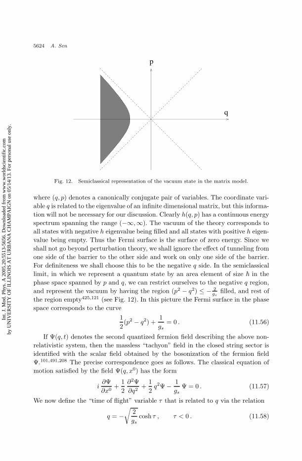
September 29, 2005 17:21 WSPC/139-IJMPA 02519
5624 A. Sen
p
q
Fig. 12. Semiclassical representation of the vacuum state in the matrix model.
where (q, p) denotes a canonically conjugate pair of variables. The coordinate vari-
able q is related to the eigenvalue of an infinite dimensional matrix, but this informa-
tion will not be necessary for our discussion. Clearly h(q, p) has a continuous energy
spectrum spanning the range (−∞,∞). The vacuum of the theory corresponds to
all states with negative h eigenvalue being filled and all states with positive h eigen-
value being empty. Thus the Fermi surface is the surface of zero energy. Since we
shall not go beyond perturbation theory, we shall ignore the effect of tunneling from
one side of the barrier to the other side and work on only one side of the barrier.
For definiteness we shall choose this to be the negative q side. In the semiclassical
limit, in which we represent a quantum state by an area element of size ~ in the
phase space spanned by p and q, we can restrict ourselves to the negative q region,
and represent the vacuum by having the region (p2 − q2) ≤ − 2gs
filled, and rest of
the region empty425,121 (see Fig. 12). In this picture the Fermi surface in the phase
space corresponds to the curve
1
2(p2 − q2) +
1
gs= 0 . (11.56)
If Ψ(q, t) denotes the second quantized fermion field describing the above non-
relativistic system, then the massless “tachyon” field in the closed string sector is
identified with the scalar field obtained by the bosonization of the fermion field
Ψ.101,491,208 The precise correspondence goes as follows. The classical equation of
motion satisfied by the field Ψ(q, x0) has the form
i∂Ψ
∂x0+
1
2
∂2Ψ
∂q2+
1
2q2Ψ − 1
gsΨ = 0 . (11.57)
We now define the “time of flight” variable τ that is related to q via the relation
q = −√
2
gscosh τ , τ < 0 . (11.58)
Int.
J. M
od. P
hys.
A 2
005.
20:5
513-
5656
. Dow
nloa
ded
from
ww
w.w
orld
scie
ntif
ic.c
omby
UN
IVE
RSI
TY
OF
ILL
INO
IS A
T U
RB
AN
A C
HA
MPA
IGN
on
05/1
4/13
. For
per
sona
l use
onl
y.
September 29, 2005 17:21 WSPC/139-IJMPA 02519
Tachyon Dynamics in Open String Theory 5625
|τ | measures the time taken by a zero energy classical particle moving under the
Hamiltonian (11.55) to travel from −√
2gs
to q. We also define
v(q) = −√
q2 − 2
gs=
√
2
gssinh τ . (11.59)
|v(q)| gives the magnitude of the classical velocity of a zero energy particle when it
is at position q. Using these variables, it is easy to see that for large negative τ the
solution to Eq. (11.57) takes the form
Ψ(q, x0) =1
√
−2v(q)
[
e−i∫
q v(q′)dq′+iπ/4ΨR(τ, x0) + ei∫
q v(q′)dq′−iπ/4ΨL(τ, x0)]
,
(11.60)
where ΨL and ΨR satisfy the field equations
(∂0 − ∂τ )ΨL(τ, x0) = 0 , (∂0 + ∂τ )ΨR(τ, x0) = 0 . (11.61)
Thus at large negative τ we can regard the system as a theory of a pair of chiral
fermions, one left-moving and the other right-moving. Of course there is an effective
boundary condition at τ = 0 which relates the two fermion fields, since a particle
coming in from τ = −∞ will be reflected from τ = 0 and will go back to τ = −∞.
Since τ ranges from 0 to −∞, we can interprete ΨR as the incoming wave and ΨL
as the outgoing wave.
Equation (11.61) shows that ΨL and ΨR represent a pair of relativistic fermions
for large negative τ . Thus we can bosonize them into a pair of chiral bosons χL
and χR. This pair of chiral bosons may in turn be combined into a full scalar
field χ(τ, x0) which satisfy the free field equation of motion for large negative τ
and satisfies an appropriate boundary condition at τ = 0. If χ is defined with the
standard normalization, then for large negative τ a single right moving fermion is
represented by the configuration93,353
χ =√πH(x0 − τ) , (11.62)
and a single left-moving fermion is represented by the configuration
χ =√πH(x0 + τ) , (11.63)
where H(u) denotes the step function defined in (11.44).
The field χ(τ, x0) is related to the tachyon field φ(ϕ, x0) in the continuum de-
scription of string theory by a nonlocal field redefinition.381 In momentum space
the relation is432,290,123,396
χ(P,E) =Γ(iP )
Γ(−iP )φ(P,E) . (11.64)
Using (11.16) this gives
χ(P,E) = ψ(P,E) , (11.65)
Int.
J. M
od. P
hys.
A 2
005.
20:5
513-
5656
. Dow
nloa
ded
from
ww
w.w
orld
scie
ntif
ic.c
omby
UN
IVE
RSI
TY
OF
ILL
INO
IS A
T U
RB
AN
A C
HA
MPA
IGN
on
05/1
4/13
. For
per
sona
l use
onl
y.
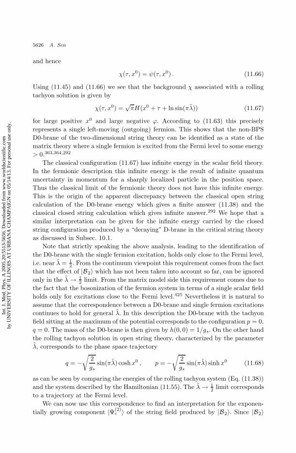
September 29, 2005 17:21 WSPC/139-IJMPA 02519
5626 A. Sen
and hence
χ(τ, x0) = ψ(τ, x0) . (11.66)
Using (11.45) and (11.66) we see that the background χ associated with a rolling
tachyon solution is given by
χ(τ, x0) =√πH(x0 + τ + ln sin(πλ)) (11.67)
for large positive x0 and large negative ϕ. According to (11.63) this precisely
represents a single left-moving (outgoing) fermion. This shows that the non-BPS
D0-brane of the two-dimensional string theory can be identified as a state of the
matrix theory where a single fermion is excited from the Fermi level to some energy
> 0.363,364,292
The classical configuration (11.67) has infinite energy in the scalar field theory.
In the fermionic description this infinite energy is the result of infinite quantum
uncertainty in momentum for a sharply localized particle in the position space.
Thus the classical limit of the fermionic theory does not have this infinite energy.
This is the origin of the apparent discrepancy between the classical open string
calculation of the D0-brane energy which gives a finite answer (11.38) and the
classical closed string calculation which gives infinite answer.292 We hope that a
similar interpretation can be given for the infinite energy carried by the closed
string configuration produced by a “decaying” D-brane in the critical string theory
as discussed in Subsec. 10.1.
Note that strictly speaking the above analysis, leading to the identification of
the D0-brane with the single fermion excitation, holds only close to the Fermi level,
i.e. near λ = 12 . From the continuum viewpoint this requirement comes from the fact
that the effect of |B2〉 which has not been taken into account so far, can be ignored
only in the λ → 12 limit. From the matrix model side this requirement comes due to
the fact that the bosonization of the fermion system in terms of a single scalar field
holds only for excitations close to the Fermi level.425 Nevertheless it is natural to
assume that the correspondence between a D0-brane and single fermion excitations
continues to hold for general λ. In this description the D0-brane with the tachyon
field sitting at the maximum of the potential corresponds to the configuration p = 0,
q = 0. The mass of the D0-brane is then given by h(0, 0) = 1/gs. On the other hand
the rolling tachyon solution in open string theory, characterized by the parameter
λ, corresponds to the phase space trajectory
q = −√
2
gssin(πλ) coshx0 , p = −
√
2
gssin(πλ) sinhx0 (11.68)
as can be seen by comparing the energies of the rolling tachyon system (Eq. (11.38))
and the system described by the Hamiltonian (11.55). The λ → 12 limit corresponds
to a trajectory at the Fermi level.
We can now use this correspondence to find an interpretation for the exponen-
tially growing component |Ψ(2)c 〉 of the string field produced by |B2〉. Since |B2〉
Int.
J. M
od. P
hys.
A 2
005.
20:5
513-
5656
. Dow
nloa
ded
from
ww
w.w
orld
scie
ntif
ic.c
omby
UN
IVE
RSI
TY
OF
ILL
INO
IS A
T U
RB
AN
A C
HA
MPA
IGN
on
05/1
4/13
. For
per
sona
l use
onl
y.
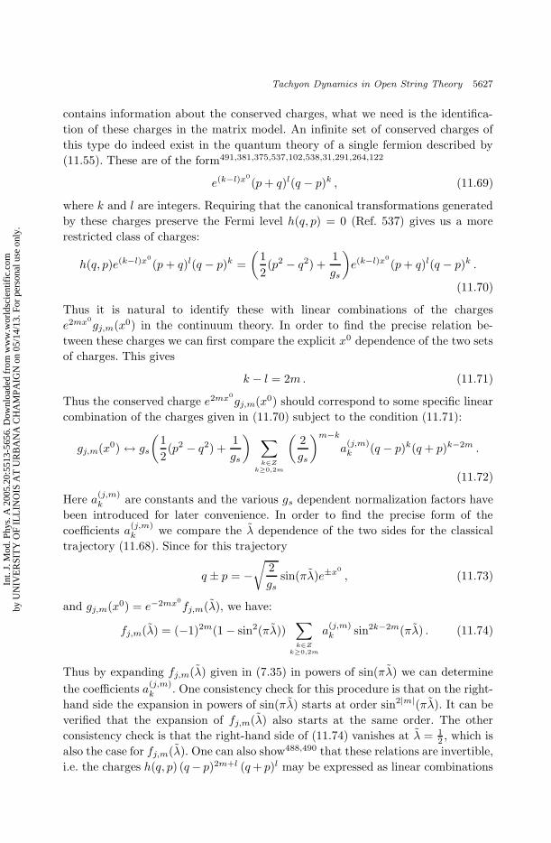
September 29, 2005 17:21 WSPC/139-IJMPA 02519
Tachyon Dynamics in Open String Theory 5627
contains information about the conserved charges, what we need is the identifica-
tion of these charges in the matrix model. An infinite set of conserved charges of
this type do indeed exist in the quantum theory of a single fermion described by
(11.55). These are of the form491,381,375,537,102,538,31,291,264,122
e(k−l)x0
(p+ q)l(q − p)k , (11.69)
where k and l are integers. Requiring that the canonical transformations generated
by these charges preserve the Fermi level h(q, p) = 0 (Ref. 537) gives us a more
restricted class of charges:
h(q, p)e(k−l)x0
(p+ q)l(q − p)k =
(
1
2(p2 − q2) +
1
gs
)
e(k−l)x0
(p+ q)l(q − p)k .
(11.70)
Thus it is natural to identify these with linear combinations of the charges
e2mx0
gj,m(x0) in the continuum theory. In order to find the precise relation be-
tween these charges we can first compare the explicit x0 dependence of the two sets
of charges. This gives
k − l = 2m. (11.71)
Thus the conserved charge e2mx0
gj,m(x0) should correspond to some specific linear
combination of the charges given in (11.70) subject to the condition (11.71):
gj,m(x0) ↔ gs
(
1
2(p2 − q2) +
1
gs
)
∑
k∈Zk≥0,2m
(
2
gs
)m−k
a(j,m)k (q − p)k(q + p)k−2m .
(11.72)
Here a(j,m)k are constants and the various gs dependent normalization factors have
been introduced for later convenience. In order to find the precise form of the
coefficients a(j,m)k we compare the λ dependence of the two sides for the classical
trajectory (11.68). Since for this trajectory
q ± p = −√
2
gssin(πλ)e±x0
, (11.73)
and gj,m(x0) = e−2mx0
fj,m(λ), we have:
fj,m(λ) = (−1)2m(1 − sin2(πλ))∑
k∈Zk≥0,2m
a(j,m)k sin2k−2m(πλ) . (11.74)
Thus by expanding fj,m(λ) given in (7.35) in powers of sin(πλ) we can determine
the coefficients a(j,m)k . One consistency check for this procedure is that on the right-
hand side the expansion in powers of sin(πλ) starts at order sin2|m|(πλ). It can be
verified that the expansion of fj,m(λ) also starts at the same order. The other
consistency check is that the right-hand side of (11.74) vanishes at λ = 12 , which is
also the case for fj,m(λ). One can also show488,490 that these relations are invertible,
i.e. the charges h(q, p) (q− p)2m+l (q+ p)l may be expressed as linear combinations
Int.
J. M
od. P
hys.
A 2
005.
20:5
513-
5656
. Dow
nloa
ded
from
ww
w.w
orld
scie
ntif
ic.c
omby
UN
IVE
RSI
TY
OF
ILL
INO
IS A
T U
RB
AN
A C
HA
MPA
IGN
on
05/1
4/13
. For
per
sona
l use
onl
y.
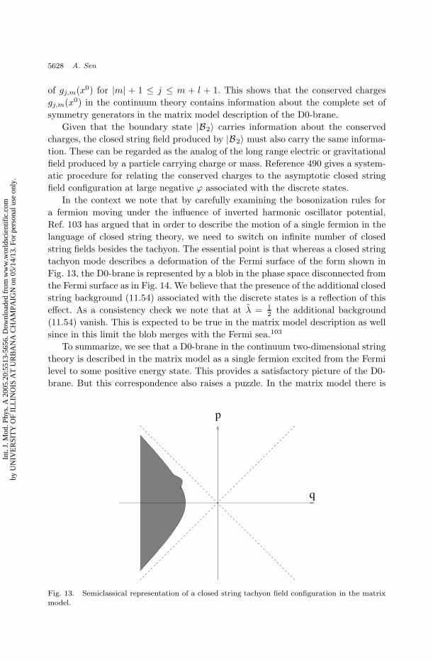
September 29, 2005 17:21 WSPC/139-IJMPA 02519
5628 A. Sen
of gj,m(x0) for |m| + 1 ≤ j ≤ m + l + 1. This shows that the conserved charges
gj,m(x0) in the continuum theory contains information about the complete set of
symmetry generators in the matrix model description of the D0-brane.
Given that the boundary state |B2〉 carries information about the conserved
charges, the closed string field produced by |B2〉 must also carry the same informa-
tion. These can be regarded as the analog of the long range electric or gravitational
field produced by a particle carrying charge or mass. Reference 490 gives a system-
atic procedure for relating the conserved charges to the asymptotic closed string
field configuration at large negative ϕ associated with the discrete states.
In the context we note that by carefully examining the bosonization rules for
a fermion moving under the influence of inverted harmonic oscillator potential,
Ref. 103 has argued that in order to describe the motion of a single fermion in the
language of closed string theory, we need to switch on infinite number of closed
string fields besides the tachyon. The essential point is that whereas a closed string
tachyon mode describes a deformation of the Fermi surface of the form shown in
Fig. 13, the D0-brane is represented by a blob in the phase space disconnected from
the Fermi surface as in Fig. 14. We believe that the presence of the additional closed
string background (11.54) associated with the discrete states is a reflection of this
effect. As a consistency check we note that at λ = 12 the additional background
(11.54) vanish. This is expected to be true in the matrix model description as well
since in this limit the blob merges with the Fermi sea.103
To summarize, we see that a D0-brane in the continuum two-dimensional string
theory is described in the matrix model as a single fermion excited from the Fermi
level to some positive energy state. This provides a satisfactory picture of the D0-
brane. But this correspondence also raises a puzzle. In the matrix model there is
p
q
Fig. 13. Semiclassical representation of a closed string tachyon field configuration in the matrixmodel.
Int.
J. M
od. P
hys.
A 2
005.
20:5
513-
5656
. Dow
nloa
ded
from
ww
w.w
orld
scie
ntif
ic.c
omby
UN
IVE
RSI
TY
OF
ILL
INO
IS A
T U
RB
AN
A C
HA
MPA
IGN
on
05/1
4/13
. For
per
sona
l use
onl
y.
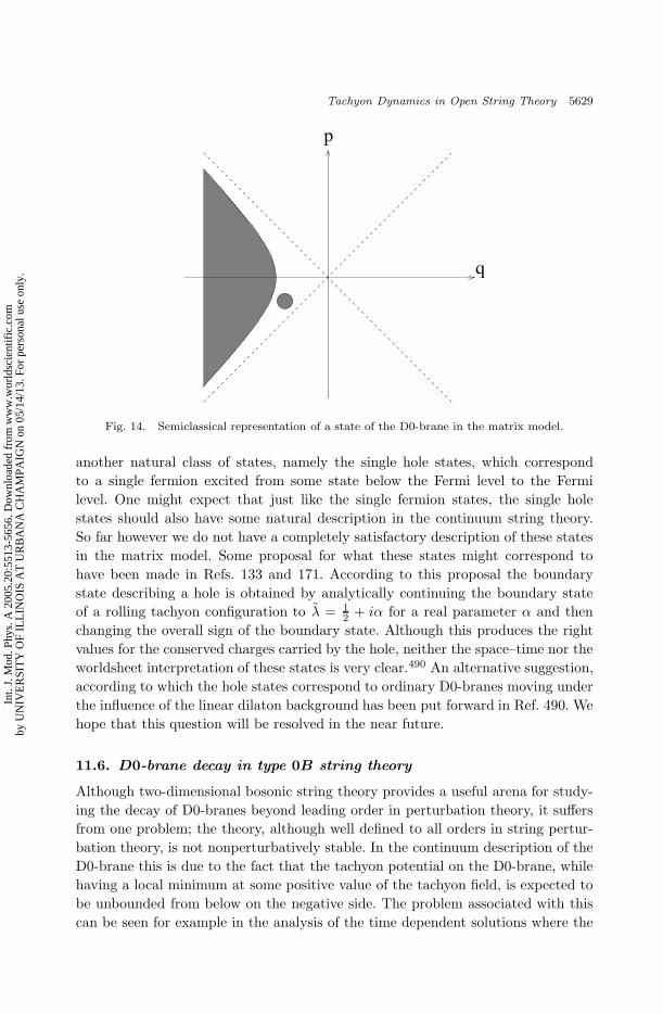
September 29, 2005 17:21 WSPC/139-IJMPA 02519
Tachyon Dynamics in Open String Theory 5629
p
q
Fig. 14. Semiclassical representation of a state of the D0-brane in the matrix model.
another natural class of states, namely the single hole states, which correspond
to a single fermion excited from some state below the Fermi level to the Fermi
level. One might expect that just like the single fermion states, the single hole
states should also have some natural description in the continuum string theory.
So far however we do not have a completely satisfactory description of these states
in the matrix model. Some proposal for what these states might correspond to
have been made in Refs. 133 and 171. According to this proposal the boundary
state describing a hole is obtained by analytically continuing the boundary state
of a rolling tachyon configuration to λ = 12 + iα for a real parameter α and then
changing the overall sign of the boundary state. Although this produces the right
values for the conserved charges carried by the hole, neither the space–time nor the
worldsheet interpretation of these states is very clear.490 An alternative suggestion,
according to which the hole states correspond to ordinary D0-branes moving under
the influence of the linear dilaton background has been put forward in Ref. 490. We
hope that this question will be resolved in the near future.
11.6. D0-brane decay in type 0B string theory
Although two-dimensional bosonic string theory provides a useful arena for study-
ing the decay of D0-branes beyond leading order in perturbation theory, it suffers
from one problem; the theory, although well defined to all orders in string pertur-
bation theory, is not nonperturbatively stable. In the continuum description of the
D0-brane this is due to the fact that the tachyon potential on the D0-brane, while
having a local minimum at some positive value of the tachyon field, is expected to
be unbounded from below on the negative side. The problem associated with this
can be seen for example in the analysis of the time dependent solutions where the
Int.
J. M
od. P
hys.
A 2
005.
20:5
513-
5656
. Dow
nloa
ded
from
ww
w.w
orld
scie
ntif
ic.c
omby
UN
IVE
RSI
TY
OF
ILL
INO
IS A
T U
RB
AN
A C
HA
MPA
IGN
on
05/1
4/13
. For
per
sona
l use
onl
y.
September 29, 2005 17:21 WSPC/139-IJMPA 02519
5630 A. Sen
tachyon rolling on the wrong side of the potential causes a divergence in the dilaton
charge at a finite time. In the matrix model description the instability is related
to the fact that the Fermi level is filled on only one side of the potential leaving
the other side empty. Such a vacuum, while perturbatively stable, is nonpertur-
batively unstable. Hence while the matrix model — two-dimensional string theory
correspondence illustrates many aspects of D0-brane decay in perturbation theory,
it does not allow us to go beyond perturbation theory.
On the matrix model side there is an easy way to solve the problem — we just fill
the Fermi level on both sides. This will have the feature that the spectrum of closed
strings, which represent excitations around the Fermi level, will be doubled since
now we can excite fermion hole pairs on either side of the potential. In particular
bosonizing the fermion field on the two sides of the potential we should either
find two different asymptotic regions with a massless scalar field living in each of
these regions, or find one asymptotic region with two massless scalar fields living
in this region. This is clearly not the two-dimensional bosonic string theory that
we have discussed so far which has only one asymptotic region (ϕ → −∞) with
one massless scalar field. Is there some other two-dimensional string theory that
corresponds to this particular matrix model? It turns out that the answer is yes: it
is two-dimensional type 0B string theory.510,133,515
The local worldsheet dynamics of type 0 string theories is identical to that of
type II string theories, i.e. it has both left and right moving worldsheet supersym-
metry. Thus the critical dimension for this theory is 10, which is equivalent to saying
the matter part of the theory must have c = 10. The difference with type II string
theories comes in the GSO projection rules. Whereas the type II string theories have
separate GSO projection on the left and the right sector, type 0 theories have one
combined GSO projection.430 Due to modular invariance this then requires that the
theory contains NS–NS and RR sector states, but no NS–R or R–NS sector states.
In other words, the closed string sector does not contain fermions! As in the case
of type II string theories, we can construct two types of type 0 string theories, 0A
and 0B, which differ from each other in the sign of the GSO projection operator in
the RR sector.
As in the case of bosonic string theory where we can construct a two-dimensional
string theory by replacing 25 of the scalar fields by a Liouville theory with total cen-
tral charge 25, we can also construct two-dimensional type 0A and 0B string theories
by replacing nine of the space-like worldsheet superfields by a super-Liouville theory.
This theory contains a single superfield with exponential potential and background
charge such that it describes a superconformal field theory with c = 9. This gives
rise to the so-called two-dimensional type 0 string theories. In particular type 0B
theory has two independent massless scalar fields in the closed string spectrum,
one coming from the RR sector and the other coming from the NS–NS sector.
Thus it is natural to conjecture that this two-dimensional string theory is equiv-
alent to the matrix model described earlier, with the two scalars being identified
with appropriate linear combinations of the excitations on the Fermi level on two
Int.
J. M
od. P
hys.
A 2
005.
20:5
513-
5656
. Dow
nloa
ded
from
ww
w.w
orld
scie
ntif
ic.c
omby
UN
IVE
RSI
TY
OF
ILL
INO
IS A
T U
RB
AN
A C
HA
MPA
IGN
on
05/1
4/13
. For
per
sona
l use
onl
y.
September 29, 2005 17:21 WSPC/139-IJMPA 02519
Tachyon Dynamics in Open String Theory 5631
sides of the potential.510,133 This is verified by computing the S-matrix involving
these fields in the type 0B theory and comparing them with the predictions of the
matrix model.123,120 The only subtle point to keep in mind is that the matrix model
Hamiltonian (11.55) seems to correspond to type 0B theory with α′ = 1/2 rather
than α′ = 1. We shall work in this unit in the rest of this section.
It turns out that the type 0B string theory has an unstable D0-brane that corre-
sponds to Dirichlet boundary condition on the Liouville coordinate, and the usual
Neumann boundary condition on the time coordinate. The open string spectrum
on this brane has a tachyonic mode. In the α′ = 1 unit the tachyon has mass2 = − 12
as in the case of unstable D-branes of superstring theory, but in the α′ = 12 unit
that we are using the tachyon has mass2 = −1. This agrees with the tachyon mass2
obtained by quantizing the inverted harmonic oscillator Hamiltonian (11.55) around
q = 0. We can also construct the rolling tachyon solution by switching on tachyon
background proportional to coshx0 or sinhx0. The worldsheet analysis is identical
to that in the case of unstable D-branes in superstring theory except for the scaling
of α′. In particular we can construct the boundary state describing this D0-brane
following the procedure discussed earlier and use this to study closed string radia-
tion from the D0-brane. The result gives a kink configuration of the type given in
Eq. (11.67) showing that the D0-brane is naturally identified with single fermion
excitations in the theory.510,133
Thus we see that we now have an example of a completely consistent two-
dimensional string theory and its matrix model description. This allows us to study
aspects of D0-brane dynamics in this theory not only to all orders in perturbation
theory but also nonperturbatively. We hope that this can be used to derive useful
insight into the dynamics of unstable D-branes in critical string theories, particu-
larly in the context of the open string completeness conjecture to be discussed in
Sec. 12.
Various other aspects of D0-brane decay in two-dimensional string theory have
been discussed in Refs. 217, 106, 12 and 266.
12. Open String Completeness Conjecture
The straightforward analysis of closed string emission from unstable D0-branes
(or Dp-branes wrapped on T p) tell us that all the energy of the D0-brane is
radiated away into closed strings, both in the critical string theory and in the two-
dimensional string theory. Naively this would suggest that the backreaction due
to the closed string emission process invalidates the classical open string results.
However we shall argue in this section that results obtained from the tree level open
string theory actually give dual description of the closed string emission process.
12.1. Open string completeness in the critical string theory
We begin our discussion by analyzing the results for D-brane decay in critical string
theory. In order to illustrate the proposed duality between open string and closed
Int.
J. M
od. P
hys.
A 2
005.
20:5
513-
5656
. Dow
nloa
ded
from
ww
w.w
orld
scie
ntif
ic.c
omby
UN
IVE
RSI
TY
OF
ILL
INO
IS A
T U
RB
AN
A C
HA
MPA
IGN
on
05/1
4/13
. For
per
sona
l use
onl
y.
September 29, 2005 17:21 WSPC/139-IJMPA 02519
5632 A. Sen
string description, let us compare the properties of the emitted closed strings from
an unstable Dp-brane wrapped on T p with those infered from the tree level open
string analysis.170,483,275,484 First of all, tree level open string analysis tells us that
the final system has:
Q/T00 = 0 , (12.1)
where Q and T00 denote the dilaton charge density and energy density of the system
respectively. On the other hand by examining the closed string worldsheet action
in the background string metric Gµν , the antisymmetric tensor field Bµν and the
dilaton ΦD at zero momentum,
Sworldsheet =1
2π
∫
d2z(Gµν(X) +Bµν(X))∂zXµ∂zX
ν , (12.2)
we see that the closed string worldsheet does not couple to the zero momentum
dilaton. This shows the final state closed strings carry zero total dilaton charge.
Hence the dilaton charge of the final state closed strings agrees with that computed
in the open string description.
Next we note that the tree level open string analysis tells us that the final
system has:
p/T00 = 0 , (12.3)
where p denotes the pressure of the system. On the other hand, closed string analysis
tells us that the final closed strings have mass m of order 1/gs, momentum k⊥transverse to the D-brane of order 1√
gsand winding w‖ tangential to the D-brane
of order 1√gs
. For such a system the ratio of transverse pressure to the energy density
is of order (k⊥/m)2 ∼ gs and the ratio of tangential pressure to the energy density
is of order −(w‖/m)2 ∼ −gs. Since both these ratios vanish in the gs → 0 limit,
we again see that the pressure of the final state closed strings match the result
computed in the open string description.
Such agreements between open and closed string results also hold for more
general cases, e.g. in the decay of unstable branes in the presence of electric field.
Consider, for example, the decay of a Dp-brane along x1, . . . , xp plane, with an
electric field e along the x1 axis. In this case the final state is characterized by its
energy–momentum tensor Tµν , source Sµν for antisymmetric tensor field Bµν and
the dilaton charge density Q. One can show that in the x0 → ∞ limit:391,448,449
T 00 = |Π|e−1δ(~x⊥) , T 11 = −|Π|eδ(~x⊥) , S01 = Πδ(~x⊥) , (12.4)
where Π is a parameter labeling the solution. All other components of Tµν and Sµν ,
as well as the dilaton charge vanishes in this limit. It can be shown that these tree
level open string results again agree exactly with the properties of the final state
closed strings into which the D-brane decays.484,219
Since in all these cases the tree level open string results for various properties
of the final state agree with the properties of the closed strings produced in the
Int.
J. M
od. P
hys.
A 2
005.
20:5
513-
5656
. Dow
nloa
ded
from
ww
w.w
orld
scie
ntif
ic.c
omby
UN
IVE
RSI
TY
OF
ILL
INO
IS A
T U
RB
AN
A C
HA
MPA
IGN
on
05/1
4/13
. For
per
sona
l use
onl
y.
September 29, 2005 17:21 WSPC/139-IJMPA 02519
Tachyon Dynamics in Open String Theory 5633
decay of the brane, we are led to conjecture that the tree level open string theory
provides a description of the rolling tachyon system which is dual to the description
in terms of closed string emission.483,484,xx,yy This is different from the usual open
closed duality where one loop open string theory contains information about closed
strings. In order to put this conjecture on a firmer footing, one must show that it
arises from a more complete conjecture involving full quantum open string theory
on an unstable D-brane. The full conjecture, suggested in Refs. 485 and 487, takes
the following form:
There is a quantum open string field theory (OSFT ) that describes the full
dynamics of an unstable Dp-brane without an explicit coupling to closed
strings. Furthermore, Ehrenfest theorem holds in the weakly coupled OSFT ;
the classical results correctly describe the time evolution of the quantum
expectation values.
Since the conjecture in essence says that quantum open string theory is fully
capable of describing the complete dynamics of an unstable D-brane, we call this
the open string completeness conjecture. Stated this way, this conjecture also em-
bodies the usual perturbative open–closed string duality for a stable D-brane where
the open string loop amplitudes contain information about closed string exchange
processes. In this case the quantum open string field theory is fully capable of
reproducing the open string scattering amplitudes at least to all orders in per-
turbation theory.192,156 For example for this system quantum open string theory
gives rise to the cylinder contribution to the string partition function at one loop
order. Coupling closed strings to this system as in Eqs. (A.4) and (A.5) will ensure
that by eliminating the closed string fields by their classical equations of motion
we get the cylinder amplitude again as in Eq. (A.8). This gives a clear indica-
tion that including closed strings in open string field theory amounts to double
counting.zz
Note that this open string completeness conjecture does not imply that the
quantum open string theory on a given system of unstable (or stable) D-branes
gives a complete description of the full string theory.aaa It only states that this
xxThis correspondence has been checked only for the space averaged values of various quantities,and not for example, for the local distribution of the various charges like the stress tensor, dilatoncharge and antisymmetric tensor field charge. This is due to the fact that we can easily give agauge invariant definition of the space-averaged quantities since they are measured by couplingto on-shell (zero momentum) closed string states, but it is more difficult to give a gauge invariantdefinition of local distribution of these charges.485yyAt present it is not clear how exactly the open string theory encodes information about closedstrings. A hint of how this might happen can be seen in the analysis of the effective fieldtheory.548,470,49,223,188,327,476,483,547 This has been reviewed briefly in Subsec. 8.3.zzIt is of course possible to construct open–closed string field theories where part of the contri-bution to a given process comes from the closed string sector and part of it comes from the openstring sector,553 but we are not discussing these theories here.aaaIn this sense it is different from the cases discussed in Ref. 197 where open string theory on aset of D-branes is completely equivalent to closed string theory on a certain background.
Int.
J. M
od. P
hys.
A 2
005.
20:5
513-
5656
. Dow
nloa
ded
from
ww
w.w
orld
scie
ntif
ic.c
omby
UN
IVE
RSI
TY
OF
ILL
INO
IS A
T U
RB
AN
A C
HA
MPA
IGN
on
05/1
4/13
. For
per
sona
l use
onl
y.
September 29, 2005 17:21 WSPC/139-IJMPA 02519
5634 A. Sen
open string field theory describes a quantum mechanically consistent subsector of
the full string theory, and is fully capable of describing the quantum dynamics of
the D-brane.bbb One of the consequences of this correspondence is that the notion
of naturalness of a solution may differ dramatically in the open and the closed
string description. A solution describing the decay of a single (or a few) unstable
D-branes may look highly contrived in the closed string description, since a generic
deformation of this background in closed string theory may not be describable by
the dynamics of a single D-brane, and may require a large (or even infinite) number
of D-branes for its description in open string theory.
In our discussion of the properties of the closed string states emitted from a
“decaying” D-brane we have so far only included closed string radiation produced
by the |B1〉 component of the boundary state. Hence our analysis is valid only in
the λ → 12 limit when the closed string background produced by |B2〉 vanishes.
As we have seen in Subsec. 10.2, for λ 6= 12 the closed string fields produced by
the |B2〉 component of the boundary state grow exponentially with time. Naively,
this exponential growth of the closed string field configurations again indicates the
breakdown of classical open string description at late time. However in the spirit
of the open string completeness conjecture proposed here it is more natural to seek
an alternative interpretation. What this may be indicating is an inadequacy of the
weakly coupled closed string description rather than an inadequacy of the open
string description. As an analogy we can cite the example of closed string field
configurations produced by static stable D-branes. Often the field configuration is
singular near the core of the brane. However we do not take this as an indication
of the breakdown of the open string description. Instead it is a reflection of the
inadequacy of the closed string description.
While in critical string theory the open string completeness remains a conjecture,
we shall see in the next subsection that this is bourne out quite clearly in the two-
dimensional string theory.
12.2. Open string completeness in two-dimensional string theory
The analysis of Subsec. 11.3 shows that a rolling tachyon configuration on a D0-
brane in two-dimensional string theory produces an infinitely sharp kink of the
closed string tachyon field. Since this carries infinite energy, we might naively con-
clude that all the energy of the D0-brane is converted to closed string radiation and
hence the results of tree level open string analysis cannot be trusted. The analysis
of Subsec. 11.4 shows that for λ 6= 12 the closed string field configuration pro-
duced by the |B2〉 component of the boundary state grows exponentially with time.
This is again a potential source for large backreaction on the tree level open string
results.
bbbFor a similar phenomenon involving stable D-branes in two-dimensional string theory seeRef. 172.
Int.
J. M
od. P
hys.
A 2
005.
20:5
513-
5656
. Dow
nloa
ded
from
ww
w.w
orld
scie
ntif
ic.c
omby
UN
IVE
RSI
TY
OF
ILL
INO
IS A
T U
RB
AN
A C
HA
MPA
IGN
on
05/1
4/13
. For
per
sona
l use
onl
y.
September 29, 2005 17:21 WSPC/139-IJMPA 02519
Tachyon Dynamics in Open String Theory 5635
On the other hand we have seen in Subsec. 11.5 that a D0-brane in two-
dimensional string theory can be identified in the matrix model description as a
single fermion excitation from the Fermi level to some energy level above 0. Since
the fermions are noninteracting, the states with a single excited fermion do not mix
with any other states in the theory (say with states where two or more fermions are
excited above the Fermi level or hole states where a fermion is excited from below
the Fermi level to the Fermi level). As a result, the quantum states of a D0-brane
are in one-to-one correspondence with the quantum states of the single particle
Hamiltonian
h(q, p) =1
2(p2 − q2) +
1
gs, (12.5)
with one additional constraint — the spectrum is cutoff sharply for energy below
zero due to Pauli exclusion principle. Since by definition quantum open string field
theory on a D-brane is a field theory that describes the dynamics of that D-brane,
we see that in the matrix model description the “quantum open string field theory”
for a single D0-brane is described by the inverted harmonic oscillator Hamiltonian
(12.5) with all the negative energy states removed by hand.485 The classical limit
of this quantum Hamiltonian is described by the classical Hamiltonian (12.5), with
a sharp cutoff on the phase space variables:ccc
1
2(p2 − q2) +
1
gs≥ 0 . (12.6)
This is the matrix model description of “classical open string field theory” describing
the dynamics of a D0-brane.ddd
Clearly the quantum system described above provides us with a complete de-
scription of the dynamics of a single D0-brane. In particular there is no need to
couple this system explicitly to closed strings, although closed strings could provide
an alternative description of the D0-brane as a kink solution in the closed string
“tachyon” field (as given in (11.67)). This is in accordance with the open string
completeness conjecture discussed in Subsec. 12.1. From this it is clear that it is a
wrong notion to think in terms of backreaction of closed string fields on the open
string dynamics. Instead we should regard the closed string background produced
by the D-brane as a way of characterizing the open string background (although the
open string theory itself is sufficient for this purpose). For example, in the present
cccThis Hamiltonian is related to the D0-brane effective Hamiltonian given in (8.13) and (8.58)by a canonical transformation485 that maps the curve h(q, p) = 0 to ∞ in the Π − T plane.dddIt will be very interesting to understand the precise connection between this system and thecubic open string field theory that describes the dynamics of the D0-brane in the continuumdescription. It will be even more interesting to study similar relation between this system andthe open string field theory describing the dynamics of the D0-brane in type 0B string theory,since there the system is nonperturbatively stable. Since on the matrix model side we have a freesystem, the approach of Refs. 201–203 might provide a useful starting point for establishing thiscorrespondence.
Int.
J. M
od. P
hys.
A 2
005.
20:5
513-
5656
. Dow
nloa
ded
from
ww
w.w
orld
scie
ntif
ic.c
omby
UN
IVE
RSI
TY
OF
ILL
INO
IS A
T U
RB
AN
A C
HA
MPA
IGN
on
05/1
4/13
. For
per
sona
l use
onl
y.
September 29, 2005 17:21 WSPC/139-IJMPA 02519
5636 A. Sen
context, we can think of the closed string tachyon field χ(τ, x0) at late time as the
expectation value of the operatoreee
χ(τ, x0) ≡ √πH
(
− q(x0) −√
2
gscosh τ
)
(12.7)
in the quantum open string theory on a single D0-brane, as described by (12.5),
(12.6). In (12.7) q denotes the position operator in the quantum open string theory.
When we calculate the expectation value of χ in the quantum state whose classical
limit is described by the trajectory (11.68), we can replace q by its classical value
q = −√
2gs
sin(πλ) cosh(x0). This gives
〈χ(τ, x0)〉 =√πH
(√
2
gssin(πλ) cosh(x0) −
√
2
gscosh τ
)
' √πH(x0 + τ + ln sin(πλ)) , (12.8)
for large x0 and negative τ . This reproduces (11.67).
In a similar spirit we note that while the naive analysis of the closed string field
configuration produced by the |B2〉 component of the boundary state indicates that
the exponentially growing closed string fields produce large backreaction and hence
invalidates the analysis based on open string theory, the results of Subsec. 11.5
clearly point to a different direction. According to these results the exponentially
growing terms in |B2〉 are simply consequences of the conserved charges a D0-brane
carries, which in turn may be calculated completely within the framework of the
open string (field) theory. Thus these exponentially growing terms do not in any
way point to an inadequacy of the open string description of D0-brane dynamics.
Various other aspects of the open string completeness conjecture in the context
of two-dimensional string theory have been discussed in Refs. 112, 11 and 352.
12.3. Generalized holographic principle
We have seen in the previous two subsections that the analysis of unstable D-brane
“decay” in critical string theory as well as in the two-dimensional string theory
points to the conjecture that the quantum open string field theory on a given D-
brane describes complete quantum dynamics of the D-brane. However generically
a given D-brane system does not have the ability to describe an arbitrary state
in string theory — it carries only partial information about the full theory.fff This
conjecture makes it clear that open string field theory on a single or a finite number
eee∂τ χ is the representation of the usual density operator of free fermions in the Hilbert space offirst quantized theory of a single fermion.fffThe possibility of using infinite number of unstable D-instantons or D0-branes or finite numberof space-filling D-branes to give a complete description of string theory has been discussed inRefs. 251, 469, 296, 27–29. Vacuum string field theory even attempts to give a complete descriptionof the theory in terms of open string field theory on a single D-brane.440,209,441
Int.
J. M
od. P
hys.
A 2
005.
20:5
513-
5656
. Dow
nloa
ded
from
ww
w.w
orld
scie
ntif
ic.c
omby
UN
IVE
RSI
TY
OF
ILL
INO
IS A
T U
RB
AN
A C
HA
MPA
IGN
on
05/1
4/13
. For
per
sona
l use
onl
y.
September 29, 2005 17:21 WSPC/139-IJMPA 02519
Tachyon Dynamics in Open String Theory 5637
of D-branes must be encoding information about the full string theory in a highly
nonlocal manner. For example when a D-brane “decays” into closed strings we
expect that at least some of the closed strings will eventually disperse to infinity.
The open string field theory, defined in terms of variables localized near the original
D-brane, must be able to describe the final closed string state produced in the decay,
although it may not be able to describe states of the individual closed strings into
which the D-brane decays. The situation can be described by drawing analogy to a
hologram. If we regard the full string theory as the complete image produced by a
hologram, then a system of finite number of D-branes can be regarded as a part of
the hologram. This encodes partial information about the full image. However the
information contained in any given piece of the hologram does not correspond to a
given part of the complete image; instead it has partial information about all parts
of the image. Thus the open string completeness conjecture proposed here can be
thought of as a generalization of the holographic principle.211,503,347,211,542,504 As
in these papers in our proposal the relation between the open and closed string
description is nonlocal, but the space in which the open string degress of freedom
live is not necessarily the boundary of the space in which the closed string degrees
of freedom live.
Acknowledgments
I would like to thank my collaborators N. Berkovits, D. Gaiotto, D. Ghoshal,
J. Majumder, N. Moeller, P. Mukhopadhyay, L. Rastelli and B. Zwiebach for col-
laboration on various aspects of open string tachyon dynamics.
Appendix A. Energy Momentum Tensor from Boundary State
As discussed in Subsec. 3.3, given a boundary CFT describing a D-brane system,
we define the corresponding boundary state |B〉 such that given any closed string
state |V 〉 and the associated vertex operator V ,
〈B|V 〉 ∝ 〈V (0)〉D , (A.1)
where 〈V (0)〉D is the one-point function of V inserted at the centre of a unit disk
D, the boundary condition/interaction on ∂D being the one associated with the
particular boundary CFT under consideration. From this definition it is clear that
the boundary state contains information about what kind of source for the closed
string states is produced by the D-brane system under consideration. In this ap-
pendix we shall make this more precise by working with (linearized) closed string
field theory.553,ggg
gggWe shall not attempt to give a detailed description of closed string field theory. Section 4 con-tains a self-contained discussion of open string field theory. Closed string field theory is formulatedon similar principles.
Int.
J. M
od. P
hys.
A 2
005.
20:5
513-
5656
. Dow
nloa
ded
from
ww
w.w
orld
scie
ntif
ic.c
omby
UN
IVE
RSI
TY
OF
ILL
INO
IS A
T U
RB
AN
A C
HA
MPA
IGN
on
05/1
4/13
. For
per
sona
l use
onl
y.
September 29, 2005 17:21 WSPC/139-IJMPA 02519
5638 A. Sen
For simplicity we shall focus on the bosonic string theory. The closed string field
corresponds to a state |Ψc〉 of ghost number 2 in the Hilbert space of matter ghost
conformal field theory in the full complex plane, satisfying the constraint553
b−0 |Ψc〉 = 0 , L−0 |Ψc〉 = 0 , (A.2)
where
c±0 = (c0 ± c0) , b±0 = (b0 ± b0) , L±0 = (L0 ± L0) . (A.3)
cn, cn, bn, bn are the usual ghost oscillators and Ln, Ln are the total Virasoro
generators. The quadratic part of the closed string field theory action can be taken
to be
− 1
Kg2s
〈Ψc|c−0 (QB + QB)|Ψc〉 , (A.4)
where QB and QB are the holomorphic and antiholomorphic components of the
BRST charge, K is a normalization constant to be determined in Eq. (A.8), and gs
is the appropriately normalized closed string coupling constant so that (2.1) holds.
In the presence of the D-brane we need to add an extra source term to the action:
〈Ψc|c−0 |B〉 . (A.5)
The equation of motion of |Ψc〉 is then
2(QB + QB)|Ψc〉 = Kg2s |B〉 . (A.6)
Clearly by a rescaling of |Ψc〉 by λ we can change K and |B〉 to K/λ2 and λ|B〉respectively. However once the normalization of |B〉 is fixed in a convenient manner,
the normalization constant K can be determined by requiring that the classical
action obtained after eliminating |Ψc〉 using its equation of motion (A.6) reproduces
the one loop partition function Zopen of the open string theory on the D-brane.
Choosing the solution of (A.6) to behhh
|Ψc〉 =1
2Kg2
sb+0 (L+
0 )−1|B〉 , (A.7)
we get
Zopen = −1
4Kg2
s〈B|b+0 c−0 (L+0 )−1|B〉 . (A.8)
We have chosen a convenient normalization of |B〉 in Eq. (3.35). This determines K
from Eq. (A.8). Since Zopen is independent of gs, and |B〉 is inversely proportional
to gs due to the T p factor in (3.35), we see that K is a purely numerical constant.
Equations (A.5) and (A.6) clearly show that |B〉 represents the source for the
closed string fields in the presence of a D-brane. We shall now make it more explicit
by expanding |Ψc〉 and |B〉 in the oscillator basis. The expansion of |Ψc〉 in the
hhhSome subtleties involved in obtaining the solution in the Minkowski space have been discussedafter Eq. (10.2).
Int.
J. M
od. P
hys.
A 2
005.
20:5
513-
5656
. Dow
nloa
ded
from
ww
w.w
orld
scie
ntif
ic.c
omby
UN
IVE
RSI
TY
OF
ILL
INO
IS A
T U
RB
AN
A C
HA
MPA
IGN
on
05/1
4/13
. For
per
sona
l use
onl
y.
September 29, 2005 17:21 WSPC/139-IJMPA 02519
Tachyon Dynamics in Open String Theory 5639
oscillator basis of closed string states has, as coefficients, various closed string fields.
For example the first few terms in the expansion are
|Ψc〉 =
∫
d26k
(2π)26
[
T (k)c1c1 + (hµν(k) + bµν(k))αµ−1α
ν−1c1c1
+
(
φ(k) +1
2ηµν hµν(k)
)
(c1c−1 − c1c−1) + · · ·]
|k〉 , (A.9)
where αµn, αµ
n are the usual oscillators associated with the Xµ fields. In this expan-
sion T (k) has the interpretation of the Fourier transform of the closed string tachyon
field, hµν = hνµ and φ(k) are Fourier transforms of the graviton (associated with
the string metric) and the dilaton fields respectively, bµν = −bνµ is the Fourier
transform of the antisymmetric tensor field, etc.iii On the other hand the boundary
state |B〉 has an expansion of the form
|B〉 =
∫
d26k
(2π)26[
F (k) + (Aµν(k) + Cµν(k))αµ−1α
ν−1
+ B(k)(b−1c−1 + b−1c−1) + · · ·]
(c0 + c0)c1c1|k〉 , (A.10)
where F , Aµν = Aνµ, Cµν = −Cνµ, B etc. are fixed functions which can be read
out of the boundary state |B〉. Substituting (A.9) and (A.10) into Eq. (A.5) we get
terms in the action proportional to∫
d26k
(2π)26[
hµν(−k)(Aµν(k) + B(k)ηµν) + 2φ(−k)B(k) + · · ·]
, (A.11)
where · · · denote source terms for other fields. Since the Fourier transform T µν of
the energy–momentum tensor couples to hµν , we see that Tµν is proportional to
Aµν(k) + ηµνB(k).jjj
We can also use an alternative but equivalent method for expressing the energy–
momentum tensor Tµν in terms of Aµν and B by using the conservation law of Tµν .
(A.6) together with nilpotence of (QB + QB) gives
(QB + QB)|B〉 = 0 . (A.12)
iiiThe identification of these fields can be found by substituting (A.9) into the quadratic action(A.4) and comparing the resulting action with the quadratic part of the known effective actioninvolving the graviton, dilaton and antisymmetric tensor field.jjjNote however that this definition of the various source terms is not unique, since we could redefinethe off-shell closed string field, and this will in general modify the source terms for various fields.A simple example of this kind is hµν(k) → f(k2)hµν(k) with f(0) = 1. This does not changethe definition of the graviton field on-shell, but modifies it off-shell. Consequently the energy–momentum tensor Tµν to which the field couples will get modified as Tµν(k) → (f(k2))−1Tµν(k).In our analysis we shall adopt the particularly simple definition of energy–momentum tensor asfollows from the action (A.4) and (A.5). In this convention the quadratic terms in the closed stringfield theory action have at most two powers of the momentum kµ. In position space this translatesto these quadratic terms having at most two derivatives. However one should keep in mind thatother choices are possible.
Int.
J. M
od. P
hys.
A 2
005.
20:5
513-
5656
. Dow
nloa
ded
from
ww
w.w
orld
scie
ntif
ic.c
omby
UN
IVE
RSI
TY
OF
ILL
INO
IS A
T U
RB
AN
A C
HA
MPA
IGN
on
05/1
4/13
. For
per
sona
l use
onl
y.
September 29, 2005 17:21 WSPC/139-IJMPA 02519
5640 A. Sen
Substituting the expansion (A.10) into this equation gives, besides other equations,
kνAµν(k) + kµB(k) = 0 . (A.13)
If Aµν(x) and B(x) denote the Fourier transforms of Aµν and B respectively,
Aµν(x) =
∫
d26k
(2π)26eik·xAµν(k) , B(x) =
∫
d26k
(2π)26eik·xB(k) , (A.14)
then (A.13) gives us
∂ν(Aµν(x) + ηµνB(x)) = 0 . (A.15)
This shows that we should identify the conserved energy–momentum tensor as
Tµν(x) ∝ (Aµν(x) + ηµνB(x)) . (A.16)
From (A.11) we also see that the function B(k) measures the source of the
dilaton field φ(k). This suggests that in position space we define the source of the
dilaton to be
Q(x) ∝ B(x) . (A.17)
Appendix B. Computation of the Energy of Closed String
Radiation from Unstable D-brane
Equation (10.12) gives the on-shell closed string field configuration produced by the
rolling tachyon background. In this appendix we shall compute the energy per unit
p-volume carried by this background. For this we express (QB + QB), acting on a
state carrying momentum kµ, as
QB + QB = (c0L0 + c0L0) + Q1(~k)k0 + Q2(~k) , (B.1)
where the operators Q1(~k) and Q2(~k) do not have any explicit k0 dependence
but can depend on the spatial components of the momentum ~k . The reason that
the right-hand side of (B.1) does not contain higher powers of k0 is that the kµ
dependence of (QB + QB) comes through the kµ dependence of the matter Vira-
soro generators L(m)n and L
(m)n , and for n 6= 0 L
(m)n and L
(m)n are linear in kµ.
Contribution from the L0 and L0 part of QB + QB , which are quadratic in kµ,
has been written separately in the right-hand side of (B.1). Let us denote by L the
part of (L0 + L0) that involves oscillator contribution and contribution from spatial
momenta, so that
L0 + L0 = −1
2(k0)2 + L . (B.2)
We also express a general closed string field configuration |Ψc〉 as
|Ψc〉 =
∫
dk0
2πψA(k0)|k0, A〉 , (B.3)
Int.
J. M
od. P
hys.
A 2
005.
20:5
513-
5656
. Dow
nloa
ded
from
ww
w.w
orld
scie
ntif
ic.c
omby
UN
IVE
RSI
TY
OF
ILL
INO
IS A
T U
RB
AN
A C
HA
MPA
IGN
on
05/1
4/13
. For
per
sona
l use
onl
y.
September 29, 2005 17:21 WSPC/139-IJMPA 02519
Tachyon Dynamics in Open String Theory 5641
where the label A runs over discrete oscillator labels as well as continuous spatial
momenta. The free closed string field theory action (A.4), expressed in terms of the
component fields ψA, takes the form
S = − 1
Kg2s
∫
dk0
2πψA(−k0)
[
− 1
2(k0)2NAB +MAB + k0M
(1)AB +M
(2)AB
]
ψB(k0) ,
(B.4)
where NAB , MAB, M(1)AB and M
(2)AB are defined through the relations
1
2〈k0, A|c−0 c+0 |k′0, B〉 = NAB2πδ(k0 + k′0) ,
1
2〈k0, A|c−0 c+0 L|k′0, B〉 = MAB2πδ(k0 + k′0) ,
〈k0, A|c−0 Q1|k′0, B〉 = M(1)AB2πδ(k0 + k′0) ,
〈k0, A|c−0 Q2|k′0, B〉 = M(2)AB2πδ(k0 + k′0) .
(B.5)
If we denote by
ψA(x0) =
∫
dk0
2πe−ik0x0
ψA(k0) , (B.6)
then the action (B.4) may be reexpressed as
S =
∫
dx0 L , (B.7)
where
L =1
Kg2s
[
1
2∂0ψANAB∂0ψB − iM
(1)ABψA∂0ψB − (MAB +M
(2)AB)ψAψB
]
. (B.8)
From this we can write down an expression for the conserved energy
E = ∂0ψA∂L
∂(∂0ψA)− L =
1
Kg2s
[
1
2∂0ψANAB∂0ψB + (MAB +M
(2)AB)ψAψB
]
. (B.9)
We shall now evaluate (B.9) for the on-shell closed string background (10.12).
For this we express |Ψ(1)c 〉 given in (10.12) as
|Ψ(1)c 〉 =
∫
dk0
2π
∑
N
∫
d25−pk⊥(2π)25−p
ψ(1)N (k0, ~k⊥)|N, ~k⊥, k
0〉 , (B.10)
where
|N, ~k⊥, k0〉 = AN c1c1
∣
∣k0, ~k‖ = 0, ~k⊥⟩
(B.11)
Int.
J. M
od. P
hys.
A 2
005.
20:5
513-
5656
. Dow
nloa
ded
from
ww
w.w
orld
scie
ntif
ic.c
omby
UN
IVE
RSI
TY
OF
ILL
INO
IS A
T U
RB
AN
A C
HA
MPA
IGN
on
05/1
4/13
. For
per
sona
l use
onl
y.
September 29, 2005 17:21 WSPC/139-IJMPA 02519
5642 A. Sen
and
ψ(1)N (k0, ~k⊥) = 2Kg2
s T pπ
sinh(
πω(N)~k⊥
)
1
2ω(N)~k⊥
×[
e−iω
(N)
~k⊥ln sin(πλ)
δ(
k0 − ω(N)~k⊥
)
+ eiω
(N)
~k⊥ln sin(πλ)
δ(
k0 + ω(N)~k⊥
)]
.
(B.12)
This gives
ψ(1)N (x0, ~k⊥) ≡
∫
dk0
2πe−ik0x0
ψN (k0, ~k⊥)
= 2Kg2s T p
π
sinh(
πω(N)~k⊥
)
1
2ω(N)~k⊥
×[
e−iω
(N)
~k⊥(x0+ln sin(πλ))
+ eiω
(N)
~k⊥(x0+ln sin(πλ))
]
. (B.13)
Using the definitions (B.3) and (B.6) of ψA(x0), definition (B.5) of NAB , MAB ,
M(1)AB and M
(2)AB , and Eq. (B.9), we can now write down an expression for the total
energy associated with the configuration |Ψ(1)c 〉 as
E(1) =1
Kg2s
∫
d25−pk⊥(2π)25−p
∑
N
[
SN∂0ψ(1)N (x0, ~k⊥)∂0ψ
(1)N (x0,−~k⊥)
+RNψ(1)N (x0, ~k⊥)ψ
(1)N (x0,−~k⊥)
]
, (B.14)
where SN and RN are defined through
1
4〈N, ~k⊥, k
0|c−0 c+0 |N, ~k ′⊥, k
′0〉
= (2π)26−pδ(k0 + k′0)δ(25−p)(~k⊥ + ~k ′⊥)SN , (B.15)
〈N, ~k⊥, k0|c−0
(
1
2c+0 L+ Q2
)
|N, ~k ′⊥, k
′0〉
= (2π)26−pδ(k0 + k′0)δ(25−p)(~k⊥ + ~k ′⊥)RN . (B.16)
From the definition of |N, ~k⊥, k0〉 and Q2 it follows that neither of them contains
a c0 or a c0 zero mode. As a result the matrix element of c−0 Q2 appearing in
(B.16) vanishes. On the other hand |N, ~k⊥〉 is an eigenstate of L with eigenvalue
2(N − 1) + 12~k2⊥ = 1
2 (ω(N)~k⊥
)2. Thus comparison of (B.15) and (B.16) gives
RN = (ω(N)~k⊥
)2SN . (B.17)
Substituting this into (B.14), and using (B.13) we get
E(1) = 4K(gsT p)2∑
N
∫
d25−pk⊥(2π)25−p
SNπ2
sinh2(
πω(N)~k⊥
) . (B.18)
Int.
J. M
od. P
hys.
A 2
005.
20:5
513-
5656
. Dow
nloa
ded
from
ww
w.w
orld
scie
ntif
ic.c
omby
UN
IVE
RSI
TY
OF
ILL
INO
IS A
T U
RB
AN
A C
HA
MPA
IGN
on
05/1
4/13
. For
per
sona
l use
onl
y.
September 29, 2005 17:21 WSPC/139-IJMPA 02519
Tachyon Dynamics in Open String Theory 5643
In order to compute SN we express the left-hand side of (B.15) as
1
4〈k0, ~k‖ = 0, ~k⊥|c−1c−1(AN )cc−0 c
+0 ANc1c1|k′0, ~k‖ = 0, ~k ′
⊥〉
=1
2V‖(2π)26−pδ(k0 + k′0)δ(25−p)(~k⊥ + ~k ′
⊥)〈0|c−1c−1(AN )cc0c0ANc1c1|0〉′′ ,(B.19)
where (AN )c is the BPZ conjugate of AN , V‖ denotes the spatial volume tangential
to the D-brane, coming from the factor of (2π)pδ(p)(~k‖) evaluated at ~k‖ = 0, and
〈·|·〉′′ denotes a renormalized BPZ inner product in the zero momentum sector such
thatkkk
〈0|c−1c−1c0c0c1c1|0〉′′ = 1 . (B.20)
This gives
SN = V‖sN , (B.21)
where
sN =1
2〈0|c−1c−1(AN )cc0c0ANc1c1|0〉′′ . (B.22)
Substituting this into (B.18) we get
E(1) = V‖E , (B.23)
where the energy per unit p-volume E is given by
E =∑
N
EN = 4K(gsT p)2∑
N
sN
∫
d25−pk⊥(2π)25−p
π2
sinh2(πω(N)~k⊥
). (B.24)
In order to compute sN using (B.22) we can use the generating functional
∑
N
sN q2(N−1) =1
2
∑
N
∑
M
〈0|c−1c−1(AN )cqL0+L0AM c1c1|0〉′′ . (B.25)
Note that only theM = N terms contribute to (B.25) due to (L0+L0) conservation.
We can now replace∑
N AN and∑
M AM by the left-hand side of (10.4). The result
is essentially the cylinder amplitude, with ln q denoting the ratio of the height to the
circumference of the cylinder. It is however well known that in this computation the
contribution from the ghost sector cancels the contribution from two of the matter
sector fields, leaving behind the contribution from 24 matter sector fields. Thus in
computing the right-hand side of (B.25) we can replace∑
N AN by
exp
[ ∞∑
n=1
24∑
s=1
(−1)ds1
nαs−nα
s−n
]
. (B.26)
kkkThis is the analog of the renormalized inner product 〈·|·〉′ for open string states as defined inEq. (4.19).
Int.
J. M
od. P
hys.
A 2
005.
20:5
513-
5656
. Dow
nloa
ded
from
ww
w.w
orld
scie
ntif
ic.c
omby
UN
IVE
RSI
TY
OF
ILL
INO
IS A
T U
RB
AN
A C
HA
MPA
IGN
on
05/1
4/13
. For
per
sona
l use
onl
y.

September 29, 2005 17:21 WSPC/139-IJMPA 02519
5644 A. Sen
We can for example take the sum over s to run over all the spatial directions tan-
gential to the brane and all the transverse directions except one. The final formula
is insensitive to ds (since ds can be changed by a redefinition αs → −αs without
changing αs), and so it does not matter whether we drop a Neumann or Dirichlet
direction in the sum over s. Using the replacement (B.26) in (B.25) the ghost term
factorises giving a contribution of q−2, and we get
∑
N
sN q2N =1
2〈0| exp
[ ∞∑
m=1
24∑
s=1
(−1)ds1
mαs
mαsm
]
qLmatter0 +Lmatter
0
× exp
[ ∞∑
n=1
24∑
r=1
(−1)dr1
nαr−nα
r−n
]
|0〉′′matter , (B.27)
where 〈·|·〉′′matter denotes the BPZ inner product in the matter sector with the nor-
malization convention 〈0|0〉′′matter = 1.
References
1. A. Abouelsaood, C. G. Callan, C. R. Nappi and S. A. Yost, Nucl. Phys. B280, 599(1987).
2. C. Acatrinei and C. Sochichiu, Phys. Rev. D67, 125017 (2003).3. A. Adams, J. Polchinski and E. Silverstein, J. High Energy Phys. 0110, 029 (2001).4. M. Aganagic, C. Popescu and J. H. Schwarz, Phys. Lett. B393, 311 (1997).5. M. Aganagic, C. Popescu and J. H. Schwarz, Nucl. Phys. B495, 99 (1997).6. M. Aganagic, R. Gopakumar, S. Minwalla and A. Strominger, J. High Energy Phys.
0104, 001 (2001).7. G. L. Alberghi, R. Casadio and A. Tronconi, J. High Energy Phys. 0406, 040 (2004).8. M. Alishahiha, H. Ita and Y. Oz, Phys. Lett. B503, 181 (2001).9. M. Alishahiha, Phys. Lett. B510, 285 (2001).
10. J. Ambjorn and R. A. Janik, Phys. Lett. B538, 189 (2002).11. J. Ambjorn and R. A. Janik, Phys. Lett. B584, 155 (2004).12. J. Ambjorn and R. A. Janik, arXiv:hep-th/0407270.13. O. Andreev, Nucl. Phys. B598, 151 (2001).14. O. Andreev and T. Ott, Nucl. Phys. B627, 330 (2002).15. O. Andreev, Phys. Lett. B534, 163 (2002).16. O. Andreev, Nucl. Phys. B680, 3 (2004).17. I. Y. Arefeva, P. B. Medvedev and A. P. Zubarev, Phys. Lett. B240, 356 (1990).18. I. Y. Arefeva, P. B. Medvedev and A. P. Zubarev, Nucl. Phys. B341, 464 (1990).19. I. Y. Arefeva, A. S. Koshelev, D. M. Belov and P. B. Medvedev, Nucl. Phys. B638,
3 (2002).20. I. Y. Arefeva, D. M. Belov, A. S. Koshelev and P. B. Medvedev, Nucl. Phys. B638,
21 (2002).21. I. Y. Arefeva, A. A. Giryavets and P. B. Medvedev, Phys. Lett. B532, 291 (2002).22. I. Y. Arefeva, D. M. Belov and A. A. Giryavets, J. High Energy Phys. 0209, 050
(2002).23. I. Y. Arefeva, A. A. Giryavets and A. S. Koshelev, Phys. Lett. B536, 138 (2002).24. I. Y. Arefeva, L. V. Joukovskaya and A. S. Koshelev, arXiv:hep-th/0301137.25. G. Arutyunov, S. Frolov, S. Theisen and A. A. Tseytlin, J. High Energy Phys. 0102,
002 (2001).
Int.
J. M
od. P
hys.
A 2
005.
20:5
513-
5656
. Dow
nloa
ded
from
ww
w.w
orld
scie
ntif
ic.c
omby
UN
IVE
RSI
TY
OF
ILL
INO
IS A
T U
RB
AN
A C
HA
MPA
IGN
on
05/1
4/13
. For
per
sona
l use
onl
y.
September 29, 2005 17:21 WSPC/139-IJMPA 02519
Tachyon Dynamics in Open String Theory 5645
26. G. Arutyunov, A. Pankiewicz and B. J. Stefanski, J. High Energy Phys. 0106, 049(2001).
27. T. Asakawa, S. Sugimoto and S. Terashima, J. High Energy Phys. 0203, 034 (2002).28. T. Asakawa, S. Sugimoto and S. Terashima, J. High Energy Phys. 0302, 011 (2003).29. T. Asakawa, S. Sugimoto and S. Terashima, Prog. Theor. Phys. Suppl. 152, 93
(2004).30. T. Asakawa, S. Kobayashi and S. Matsuura, J. High Energy Phys. 0310, 023 (2003).31. J. Avan and A. Jevicki, Nucl. Phys. B397, 672 (1993).32. V. Balasubramanian, E. Keski-Vakkuri, P. Kraus and A. Naqvi, arXiv:hep-
th/0404039.33. R. Banerjee, Y. Kim and O. K. Kwon, arXiv:hep-th/0407229.34. T. Banks and L. Susskind, arXiv:hep-th/9511194.35. K. Bardakci, Nucl. Phys. B68, 331 (1974).36. K. Bardakci and M. B. Halpern, Nucl. Phys. B73, 295 (1974).37. K. Bardakci, Nucl. Phys. B133, 297 (1978).38. K. Bardakci and A. Konechny, arXiv:hep-th/0105098.39. N. Barnaby, J. High Energy Phys. 0407, 025 (2004).40. N. Barnaby and J. M. Cline, arXiv:hep-th/0410030.41. I. Bars, H. Kajiura, Y. Matsuo and T. Takayanagi, Phys. Rev. D63, 086001 (2001).42. I. Bars, I. Kishimoto and Y. Matsuo, Phys. Rev. D67, 126007 (2003).43. D. Bazeia, R. Menezes and J. G. Ramos, arXiv:hep-th/0401195.44. O. Bergman and M. R. Gaberdiel, Phys. Lett. B441, 133 (1998).45. O. Bergman and M. R. Gaberdiel, J. High Energy Phys. 9903, 013 (1999).46. O. Bergman, E. G. Gimon and P. Horava, J. High Energy Phys. 9904, 010 (1999).47. O. Bergman and M. R. Gaberdiel, Class. Quantum Grav. 17, 961 (2000).48. O. Bergman, J. High Energy Phys. 0011, 015 (2000).49. O. Bergman, K. Hori and P. Yi, Nucl. Phys. B580, 289 (2000).50. O. Bergman and S. S. Razamat, arXiv:hep-th/0402124.51. E. Bergshoeff and P. K. Townsend, Nucl. Phys. B490, 145 (1997).52. E. A. Bergshoeff, M. de Roo, T. C. de Wit, E. Eyras and S. Panda, J. High Energy
Phys. 0005, 009 (2000).53. N. Berkovits, M. T. Hatsuda and W. Siegel, Nucl. Phys. B371, 434 (1992).54. N. Berkovits, Nucl. Phys. B450, 90 (1995) [Erratum, ibid. B459, 439 (1996)].55. N. Berkovits, Fortsch. Phys. 48, 31 (2000).56. N. Berkovits, J. High Energy Phys. 0004, 022 (2000).57. N. Berkovits, A. Sen and B. Zwiebach, Nucl. Phys. B587, 147 (2000).58. N. Berkovits, arXiv:hep-th/0105230.59. N. Berkovits, J. High Energy Phys. 0111, 047 (2001).60. S. Bhattacharya, S. Mukherji and S. Roy, Phys. Lett. B584, 163 (2004).61. L. Bonora, D. Mamone and M. Salizzoni, Nucl. Phys. B630, 163 (2002).62. L. Bonora, D. Mamone and M. Salizzoni, J. High Energy Phys. 0204, 020 (2002).63. L. Bonora, D. Mamone and M. Salizzoni, J. High Energy Phys. 0301, 013 (2003).64. L. Bonora, C. Maccaferri, D. Mamone and M. Salizzoni, arXiv:hep-th/0304270.65. L. Bonora, C. Maccaferri and P. Prester, J. High Energy Phys. 0401, 038 (2004).66. L. Bonora, C. Maccaferri and P. Prester, arXiv:hep-th/0404154.67. L. Bonora, C. Maccaferri, R. J. S. Santos and D. D. Tolla, arXiv:hep-th/0409063.68. P. Bouwknegt and V. Mathai, J. High Energy Phys. 0003, 007 (2000).69. P. Brax, G. Mandal and Y. Oz, Phys. Rev. D63, 064008 (2001).70. P. Brax, J. Mourad and D. A. Steer, arXiv:hep-th/0304197.71. P. Brax, J. Mourad and D. A. Steer, arXiv:hep-th/0310079.
Int.
J. M
od. P
hys.
A 2
005.
20:5
513-
5656
. Dow
nloa
ded
from
ww
w.w
orld
scie
ntif
ic.c
omby
UN
IVE
RSI
TY
OF
ILL
INO
IS A
T U
RB
AN
A C
HA
MPA
IGN
on
05/1
4/13
. For
per
sona
l use
onl
y.
September 29, 2005 17:21 WSPC/139-IJMPA 02519
5646 A. Sen
72. L. Brekke, P. G. O. Freund, M. Olson and E. Witten, Nucl. Phys. B302, 365 (1988).73. E. Brezin, V. A. Kazakov and A. B. Zamolodchikov, Nucl. Phys. B338, 673 (1990).74. A. Buchel, P. Langfelder and J. Walcher, Ann. Phys. 302, 78 (2002).75. A. Buchel and J. Walcher, Fortsch. Phys. 51, 885 (2003).76. A. Buchel and J. Walcher, J. High Energy Phys. 0305, 069 (2003).77. C. P. Burgess, M. Majumdar, D. Nolte, F. Quevedo, G. Rajesh and R. J. Zhang,
J. High Energy Phys. 0107, 047 (2001).78. C. G. Callan, C. Lovelace, C. R. Nappi and S. A. Yost, Nucl. Phys. B293, 83 (1987).79. C. G. Callan, I. R. Klebanov, A. W. W. Ludwig and J. M. Maldacena, Nucl. Phys.
B422, 417 (1994).80. M. Cederwall, A. von Gussich, B. E. W. Nilsson and A. Westerberg, Nucl. Phys.
B490, 163 (1997).81. M. Cederwall, A. von Gussich, B. E. W. Nilsson, P. Sundell and A. Westerberg,
Nucl. Phys. B490, 179 (1997).82. G. Chalmers, J. High Energy Phys. 0106, 012 (2001).83. B. Chen and F. L. Lin, Phys. Rev. D66, 126001 (2002).84. B. Chen, M. Li and F. L. Lin, J. High Energy Phys. 0211, 050 (2002).85. C. M. Chen, D. V. Gal’tsov and M. Gutperle, Phys. Rev. D66, 024043 (2002).86. T. Chen, J. Frohlich and J. Walcher, Commun. Math. Phys. 237, 243 (2003).87. X. G. Chen, arXiv:hep-th/0311179.88. T. E. Clark, M. Nitta and T. ter Veldhuis, Phys. Rev. D69, 047701 (2004).89. T. E. Clark, M. Nitta and T. ter Veldhuis, arXiv:hep-th/0401163.90. T. E. Clark, M. Nitta and T. ter Veldhuis, arXiv:hep-th/0409030.91. T. E. Clark, M. Nitta and T. ter Veldhuis, arXiv:hep-th/0409151.92. J. M. Cline and H. Firouzjahi, Phys. Lett. B564, 255 (2003).93. S. R. Coleman, Phys. Rev. D11, 2088 (1975).94. N. R. Constable and F. Larsen, arXiv:hep-th/0305177.95. E. J. Copeland, P. M. Saffin and D. A. Steer, Phys. Rev. D68, 065013 (2003).96. S. Corley and S. Ramgoolam, J. High Energy Phys. 0103, 037 (2001).97. L. Cornalba, Phys. Lett. B504, 55 (2001).98. B. Craps, P. Kraus and F. Larsen, J. High Energy Phys. 0106, 062 (2001).99. B. C. da Cunha, arXiv:hep-th/0403217.
100. J. Dai, R. Leigh and J. Polchinski, Mod. Phys. Lett. A4, 2073 (1989).101. S. R. Das and A. Jevicki, Mod. Phys. Lett. A5, 1639 (1990).102. S. R. Das, A. Dhar, G. Mandal and S. R. Wadia, Int. J. Mod. Phys. A7, 5165 (1992).103. S. R. Das, arXiv:hep-th/0401067.104. K. Dasgupta, S. Mukhi and G. Rajesh, J. High Energy Phys. 0006, 022 (2000).105. S. Dasgupta and T. Dasgupta, J. High Energy Phys. 0106, 007 (2001).106. S. Dasgupta and T. Dasgupta, arXiv:hep-th/0310106.107. F. David, Mod. Phys. Lett. A3, 1651 (1988).108. J. R. David, J. High Energy Phys. 0107, 009 (2001).109. J. R. David, J. High Energy Phys. 0107, 024 (2001).110. J. R. David, J. High Energy Phys. 0010, 004 (2000).111. S. P. de Alwis and A. T. Flournoy, Phys. Rev. D63, 106001 (2001).112. J. de Boer, A. Sinkovics, E. Verlinde and J. T. Yee, J. High Energy Phys. 0403, 023
(2004).113. R. de Mello Koch, A. Jevicki, M. Mihailescu and R. Tatar, Phys. Lett. B482, 249
(2000).114. R. de Mello Koch and J. P. Rodrigues, Phys. Lett. B495, 237 (2000).115. P. J. De Smet and J. Raeymaekers, J. High Energy Phys. 0107, 032 (2001).
Int.
J. M
od. P
hys.
A 2
005.
20:5
513-
5656
. Dow
nloa
ded
from
ww
w.w
orld
scie
ntif
ic.c
omby
UN
IVE
RSI
TY
OF
ILL
INO
IS A
T U
RB
AN
A C
HA
MPA
IGN
on
05/1
4/13
. For
per
sona
l use
onl
y.
September 29, 2005 17:21 WSPC/139-IJMPA 02519
Tachyon Dynamics in Open String Theory 5647
116. P. J. De Smet, arXiv:hep-th/0109182.117. P. J. De Smet and J. Raeymaekers, J. High Energy Phys. 0005, 051 (2000).118. P. De Smet and J. Raeymaekers, J. High Energy Phys. 0008, 020 (2000).119. Y. Demasure and R. A. Janik, Phys. Lett. B578, 195 (2004).120. O. DeWolfe, R. Roiban, M. Spradlin, A. Volovich and J. Walcher, J. High Energy
Phys. 0311, 012 (2003).121. A. Dhar, G. Mandal and S. R. Wadia, Int. J. Mod. Phys. A8, 3811 (1993).122. A. Dhar, G. Mandal and S. R. Wadia, Nucl. Phys. B454, 541 (1995).123. P. Di Francesco and D. Kutasov, Nucl. Phys. B375, 119 (1992).124. R. Dijkgraaf, E. Verlinde and H. Verlinde, Commun. Math. Phys. 115, 649 (1988).125. J. Distler and H. Kawai, Nucl. Phys. B321, 509 (1989).126. P. Di Vecchia, M. Frau, I. Pesando, S. Sciuto, A. Lerda and R. Russo, Nucl. Phys.
B507, 259 (1997).127. P. Di Vecchia and A. Liccardo, arXiv:hep-th/9912275.128. E. E. Donets, A. P. Isaev, C. Sochichiu and M. Tsulaia, J. High Energy Phys. 0012,
022 (2000).129. H. Dorn and H. J. Otto, Phys. Lett. B291, 39 (1992).130. H. Dorn and H. J. Otto, Nucl. Phys. B429, 375 (1994).131. M. R. Douglas and C. M. Hull, J. High Energy Phys. 9802, 008 (1998).132. M. R. Douglas, H. Liu, G. W. Moore and B. Zwiebach, J. High Energy Phys. 0204,
022 (2002).133. M. R. Douglas, I. R. Klebanov, D. Kutasov, J. Maldacena, E. Martinec and N.
Seiberg, arXiv:hep-th/0307195.134. N. Drukker, D. J. Gross and N. Itzhaki, Phys. Rev. D62, 086007 (2000).135. N. Drukker, J. High Energy Phys. 0308, 017 (2003).136. G. R. Dvali and S. H. H. Tye, Phys. Lett. B450, 72 (1999).137. G. R. Dvali, Q. Shafi and S. Solganik, arXiv:hep-th/0105203.138. I. Ellwood and W. Taylor, Phys. Lett. B512, 181 (2001).139. I. Ellwood, B. Feng, Y. H. He and N. Moeller, J. High Energy Phys. 0107, 016
(2001).140. I. Ellwood and W. Taylor, arXiv:hep-th/0105156.141. T. G. Erler and D. J. Gross, arXiv:hep-th/0406199.142. T. G. Erler, arXiv:hep-th/0409179.143. E. Eyras, J. High Energy Phys. 9910, 005 (1999).144. G. N. Felder, L. Kofman and A. Starobinsky, J. High Energy Phys. 0209, 026 (2002).145. G. N. Felder and L. Kofman, Phys. Rev. D70, 046004 (2004).146. P. Fendley, H. Saleur and N. P. Warner, Nucl. Phys. B430, 577 (1994).147. B. Feng, Y. H. He and N. Moeller, arXiv:hep-th/0103103.148. A. Fotopoulos and A. A. Tseytlin, J. High Energy Phys. 0312, 025 (2003).149. P. H. Frampton and Y. Okada, Phys. Rev. Lett. 60, 484 (1988).150. P. H. Frampton and Y. Okada, Phys. Rev. D37, 3077 (1988).151. M. Frau, L. Gallot, A. Lerda and P. Strigazzi, Nucl. Phys. B564, 60 (2000).152. S. Fredenhagen and V. Schomerus, J. High Energy Phys. 0104, 007 (2001).153. S. Fredenhagen and V. Schomerus, arXiv:hep-th/0308205.154. P. G. O. Freund and M. Olson, Phys. Lett. B199, 186 (1987).155. P. G. O. Freund and E. Witten, Phys. Lett. B199, 191 (1987).156. D. Z. Freedman, S. B. Giddings, J. A. Shapiro and C. B. Thorn, Nucl. Phys. B298,
253 (1988).157. D. Friedan, S. H. Shenker and E. J. Martinec, Phys. Lett. B160, 55 (1985).158. D. Friedan, E. J. Martinec and S. H. Shenker, Nucl. Phys. B271, 93 (1986).
Int.
J. M
od. P
hys.
A 2
005.
20:5
513-
5656
. Dow
nloa
ded
from
ww
w.w
orld
scie
ntif
ic.c
omby
UN
IVE
RSI
TY
OF
ILL
INO
IS A
T U
RB
AN
A C
HA
MPA
IGN
on
05/1
4/13
. For
per
sona
l use
onl
y.
September 29, 2005 17:21 WSPC/139-IJMPA 02519
5648 A. Sen
159. E. Fuchs, M. Kroyter and A. Marcus, J. High Energy Phys. 0209, 022 (2002).160. M. Fujita and H. Hata, arXiv:hep-th/0304163.161. M. Fujita and H. Hata, arXiv:hep-th/0403031.162. M. R. Gaberdiel and B. J. Stefanski, Nucl. Phys. B578, 58 (2000).163. M. R. Gaberdiel, Class. Quantum Grav. 17, 3483 (2000).164. M. R. Gaberdiel, A. Recknagel and G. M. T. Watts, Nucl. Phys. B626, 344 (2002).165. M. R. Gaberdiel and A. Recknagel, J. High Energy Phys. 0111, 016 (2001).166. D. Gaiotto, L. Rastelli, A. Sen and B. Zwiebach, Adv. Theor. Math. Phys. 6, 403
(2003).167. D. Gaiotto, L. Rastelli, A. Sen and B. Zwiebach, J. High Energy Phys. 0203, 003
(2002).168. D. Gaiotto, L. Rastelli, A. Sen and B. Zwiebach, J. High Energy Phys. 0204, 060
(2002).169. D. Gaiotto and L. Rastelli, J. High Energy Phys. 0308, 048 (2003).170. D. Gaiotto, N. Itzhaki and L. Rastelli, arXiv:hep-th/0304192.171. D. Gaiotto, N. Itzhaki and L. Rastelli, Phys. Lett. B575, 111 (2003).172. D. Gaiotto and L. Rastelli, arXiv:hep-th/0312196.173. H. Garcia-Compean, Nucl. Phys. B557, 480 (1999).174. M. R. Garousi, Nucl. Phys. B584, 284 (2000).175. M. R. Garousi, Nucl. Phys. B647, 117 (2002).176. M. R. Garousi, J. High Energy Phys. 0304, 027 (2003).177. M. R. Garousi, Nucl. Phys. B584, 284 (2000); J. High Energy Phys. 0305, 058
(2003).178. M. R. Garousi, J. High Energy Phys. 0312, 036 (2003).179. E. Gava, K. S. Narain and M. H. Sarmadi, Nucl. Phys. B504, 214 (1997).180. A. A. Gerasimov and S. L. Shatashvili, J. High Energy Phys. 0010, 034 (2000).181. A. A. Gerasimov and S. L. Shatashvili, J. High Energy Phys. 0101, 019 (2001).182. A. A. Gerasimov and S. L. Shatashvili, J. High Energy Phys. 0106, 066 (2001).183. D. Ghoshal and A. Sen, Nucl. Phys. B584, 300 (2000).184. D. Ghoshal and A. Sen, J. High Energy Phys. 0011, 021 (2000).185. D. Ghoshal, arXiv:hep-th/0106231.186. D. Ghoshal, arXiv:hep-th/0406259.187. D. Ghoshal and T. Kawano, arXiv:hep-th/0409311.188. G. W. Gibbons, K. Hori and P. Yi, Nucl. Phys. B596, 136 (2001).189. G. Gibbons, K. Hashimoto and P. Yi, J. High Energy Phys. 0209, 061 (2002).190. G. W. Gibbons, Phys. Lett. B537, 1 (2002).191. S. B. Giddings, Nucl. Phys. B278, 242 (1986).192. S. B. Giddings, E. J. Martinec and E. Witten, Phys. Lett. B176, 362 (1986).193. P. Ginsparg and J. Zinn-Justin, Phys. Lett. B240, 333 (1990).194. S. Giusto and C. Imbimbo, Nucl. Phys. B677, 52 (2004).195. C. Gomez and P. Resco, arXiv:hep-th/0106195.196. C. Gomez and J. J. Manjarin, arXiv:hep-th/0111169.197. R. Gopakumar and C. Vafa, Adv. Theor. Math. Phys. 3, 1415 (1999).198. R. Gopakumar, S. Minwalla and A. Strominger, J. High Energy Phys. 0005, 020
(2000).199. R. Gopakumar, S. Minwalla and A. Strominger, hep-th/0007226.200. R. Gopakumar, M. Headrick and M. Spradlin, Commun. Math. Phys. 233, 355
(2003).201. R. Gopakumar, Phys. Rev. D70, 025009 (2004).202. R. Gopakumar, Phys. Rev. D70, 025010 (2004).
Int.
J. M
od. P
hys.
A 2
005.
20:5
513-
5656
. Dow
nloa
ded
from
ww
w.w
orld
scie
ntif
ic.c
omby
UN
IVE
RSI
TY
OF
ILL
INO
IS A
T U
RB
AN
A C
HA
MPA
IGN
on
05/1
4/13
. For
per
sona
l use
onl
y.
September 29, 2005 17:21 WSPC/139-IJMPA 02519
Tachyon Dynamics in Open String Theory 5649
203. R. Gopakumar, arXiv:hep-th/0409233.204. M. B. Green, Phys. Lett. B329, 435 (1994).205. M. B. Green and M. Gutperle, Nucl. Phys. B476, 484 (1996).206. G. Grignani, M. Laidlaw, M. Orselli and G. W. Semenoff, Phys. Lett. B543, 127
(2002).207. D. J. Gross and N. Miljkovic, Phys. Lett. B238, 217 (1990).208. D. J. Gross and I. R. Klebanov, Nucl. Phys. B352, 671 (1991).209. D. J. Gross and W. Taylor, J. High Energy Phys. 0108, 009 (2001).210. D. J. Gross and W. Taylor, J. High Energy Phys. 0108, 010 (2001).211. S. S. Gubser, I. R. Klebanov and A. M. Polyakov, Phys. Lett. B428, 105 (1998).212. S. Gukov, Commun. Math. Phys. 210, 621 (2000).213. Z. Guralnik and S. Ramgoolam, J. High Energy Phys. 0102, 032 (2001).214. H. Gustafsson and U. Lindstrom, Phys. Lett. B440, 43 (1998).215. M. Gutperle and A. Strominger, J. High Energy Phys. 0204, 018 (2002).216. M. Gutperle and A. Strominger, Phys. Rev. D67, 126002 (2003).217. M. Gutperle and P. Kraus, Phys. Rev. D69, 066005 (2004).218. M. Gutperle and W. Sabra, arXiv:hep-th/0407147.219. M. Gutperle and P. Yi, arXiv:hep-th/0409050.220. J. A. Harvey, P. Horava and P. Kraus, J. High Energy Phys. 0003, 021 (2000).221. J. A. Harvey and P. Kraus, J. High Energy Phys. 0004, 012 (2000).222. J. A. Harvey, D. Kutasov and E. J. Martinec, arXiv:hep-th/0003101.223. J. A. Harvey, P. Kraus, F. Larsen and E. J. Martinec, J. High Energy Phys. 0007,
042 (2000).224. J. A. Harvey, P. Kraus and F. Larsen, Phys. Rev. D63, 026002 (2001).225. J. A. Harvey and G. W. Moore, J. Math. Phys. 42, 2765 (2001).226. J. A. Harvey, P. Kraus and F. Larsen, hep-th/0010060.227. J. A. Harvey, arXiv:hep-th/0102076.228. A. Hashimoto and W. I. Taylor, Nucl. Phys. B503, 193 (1997).229. A. Hashimoto and N. Itzhaki, J. High Energy Phys. 0201, 028 (2002).230. K. Hashimoto and K. Krasnov, Phys. Rev. D64, 046007 (2001).231. K. Hashimoto and S. Hirano, Phys. Rev. D65, 026006 (2002).232. K. Hashimoto and S. Nagaoka, Phys. Rev. D66, 026001 (2002).233. K. Hashimoto, J. High Energy Phys. 0207, 035 (2002).234. K. Hashimoto and N. Sakai, J. High Energy Phys. 0212, 064 (2002).235. K. Hashimoto, P. M. Ho and J. E. Wang, Phys. Rev. Lett. 90, 141601 (2003).236. K. Hashimoto, P. M. Ho, S. Nagaoka and J. E. Wang, Phys. Rev. D68, 026007
(2003).237. K. Hashimoto and S. Nagaoka, J. High Energy Phys. 0306, 034 (2003).238. K. Hashimoto and S. Terashima, J. High Energy Phys. 0406, 048 (2004).239. H. Hata and S. Shinohara, J. High Energy Phys. 0009, 035 (2000).240. H. Hata and S. Teraguchi, J. High Energy Phys. 0105, 045 (2001).241. H. Hata and T. Kawano, J. High Energy Phys. 0111, 038 (2001).242. H. Hata and S. Moriyama, J. High Energy Phys. 0201, 042 (2002).243. H. Hata, S. Moriyama and S. Teraguchi, J. High Energy Phys. 0202, 036 (2002).244. H. Hata and S. Moriyama, Nucl. Phys. B651, 3 (2003).245. H. Hata and H. Kogetsu, J. High Energy Phys. 0209, 027 (2002).246. H. Hata, H. Kogetsu and S. Teraguchi, J. High Energy Phys. 0402, 045 (2004).247. M. Headrick, S. Minwalla and T. Takayanagi, Class. Quantum Grav. 21, S1539
(2004).248. Y. Hikida, M. Nozaki and T. Takayanagi, Nucl. Phys. B595, 319 (2001).
Int.
J. M
od. P
hys.
A 2
005.
20:5
513-
5656
. Dow
nloa
ded
from
ww
w.w
orld
scie
ntif
ic.c
omby
UN
IVE
RSI
TY
OF
ILL
INO
IS A
T U
RB
AN
A C
HA
MPA
IGN
on
05/1
4/13
. For
per
sona
l use
onl
y.
September 29, 2005 17:21 WSPC/139-IJMPA 02519
5650 A. Sen
249. Y. Hikida, M. Nozaki and Y. Sugawara, Nucl. Phys. B617, 117 (2001).250. G. ’t Hooft, Nucl. Phys. B79, 276 (1974).251. P. Horava, Adv. Theor. Math. Phys. 2, 1373 (1999).252. W. H. Huang, Phys. Lett. B561, 153 (2003).253. W. H. Huang, J. High Energy Phys. 0408, 060 (2004).254. Y. Imamura, J. High Energy Phys. 0207, 042 (2002).255. A. Iqbal and A. Naqvi, arXiv:hep-th/0004015.256. A. Iqbal and A. Naqvi, J. High Energy Phys. 0101, 040 (2001).257. N. Ishibashi, Mod. Phys. Lett. A4, 251 (1989).258. A. Ishida and S. Uehara, Phys. Lett. B544, 353 (2002).259. A. Ishida and S. Uehara, J. High Energy Phys. 0302, 050 (2003).260. J. M. Isidro, J. Geom. Phys. 42, 325 (2002).261. D. P. Jatkar, G. Mandal and S. R. Wadia, J. High Energy Phys. 0009, 018 (2000).262. D. P. Jatkar and R. Vathsan, J. High Energy Phys. 0106, 039 (2001).263. D. P. Jatkar, S. Sur and R. Vathsan, Phys. Lett. B520, 391 (2001).264. A. Jevicki, arXiv:hep-th/9302106.265. C. V. Johnson, arXiv:hep-th/0007170.266. C. V. Johnson, arXiv:hep-th/0408049.267. G. Jones, A. Maloney and A. Strominger, Phys. Rev. D69, 126008 (2004).268. N. T. Jones and S. H. H. Tye, J. High Energy Phys. 0301, 012 (2003).269. G. Jorjadze and G. Weigt, arXiv:hep-th/0207041.270. G. Jorjadze and G. Weigt, Phys. Lett. B581, 133 (2004).271. L. Joukovskaya and Y. Volovich, arXiv:math-ph/0308034.272. H. Kajiura, Y. Matsuo and T. Takayanagi, J. High Energy Phys. 0106, 041 (2001).273. K. Kamimura and J. Simon, Nucl. Phys. B585, 219 (2000).274. S. Kar, arXiv:hep-th/0210108.275. J. L. Karczmarek, H. Liu, J. Maldacena and A. Strominger, arXiv:hep-th/0306132.276. F. Katsumata, T. Takahashi and S. Zeze, arXiv:hep-th/0409249.277. H. Kawai and T. Kuroki, Phys. Lett. B518, 294 (2001).278. T. Kawano and T. Takahashi, hep-th/9912274.279. C. Kennedy and A. Wilkins, Phys. Lett. B464, 206 (1999).280. C. J. Kim, H. B. Kim, Y. B. Kim and O. K. Kwon, J. High Energy Phys. 0303, 008
(2003).281. C. J. Kim, Y. B. Kim and C. O. Lee, J. High Energy Phys. 0305, 020 (2003).282. C. Kim, Y. Kim, O. K. Kwon and C. O. Lee, J. High Energy Phys. 0311, 034 (2003).283. C. J. Kim, Y. B. Kim, O. K. Kwon and P. Yi, J. High Energy Phys. 0309, 042
(2003).284. C. Kim, Y. Kim and O. K. Kwon, J. High Energy Phys. 0405, 020 (2004).285. H. Kim, J. High Energy Phys. 0301, 080 (2003).286. I. Kishimoto, J. High Energy Phys. 0112, 007 (2001).287. I. Kishimoto and K. Ohmori, J. High Energy Phys. 0205, 036 (2002).288. I. Kishimoto and T. Takahashi, Prog. Theor. Phys. 108, 591 (2002).289. M. Kleban, A. Lawrence and S. Shenker, hep-th/0012081.290. I. R. Klebanov, arXiv:hep-th/9108019.291. I. R. Klebanov and A. Pasquinucci, arXiv:hep-th/9210105.292. I. R. Klebanov, J. Maldacena and N. Seiberg, J. High Energy Phys. 0307, 045 (2003).293. A. Kling, O. Lechtenfeld, A. D. Popov and S. Uhlmann, Phys. Lett. B551, 193
(2003).294. A. Kling, O. Lechtenfeld, A. D. Popov and S. Uhlmann, Fortsch. Phys. 51, 775
(2003).
Int.
J. M
od. P
hys.
A 2
005.
20:5
513-
5656
. Dow
nloa
ded
from
ww
w.w
orld
scie
ntif
ic.c
omby
UN
IVE
RSI
TY
OF
ILL
INO
IS A
T U
RB
AN
A C
HA
MPA
IGN
on
05/1
4/13
. For
per
sona
l use
onl
y.
September 29, 2005 17:21 WSPC/139-IJMPA 02519
Tachyon Dynamics in Open String Theory 5651
295. J. Kluson, Phys. Rev. D62, 126003 (2000).296. J. Kluson, J. High Energy Phys. 0011, 016 (2000).297. J. Kluson, J. High Energy Phys. 0103, 018 (2001).298. J. Kluson, Phys. Rev. D64, 126006 (2001).299. J. Kluson, arXiv:hep-th/0208028.300. J. Kluson, J. High Energy Phys. 0311, 068 (2003).301. J. Kluson, J. High Energy Phys. 0401, 019 (2004).302. J. Kluson, J. High Energy Phys. 0402, 024 (2004).303. J. Kluson, J. High Energy Phys. 0406, 021 (2004).304. V. G. Knizhnik, A. M. Polyakov and A. B. Zamolodchikov, Mod. Phys. Lett. A3,
819 (1988).305. S. Kobayashi, T. Asakawa and S. Matsuura, arXiv:hep-th/0409044.306. A. Koshelev, arXiv:hep-th/0212055.307. V. A. Kostelecky and S. Samuel, Phys. Lett. B207, 169 (1988).308. V. A. Kostelecky and S. Samuel, Nucl. Phys. B336, 263 (1990).309. V. A. Kostelecky and R. Potting, Phys. Lett. B381, 89 (1996).310. V. A. Kostelecky and R. Potting, Phys. Rev. D63, 046007 (2001).311. T. Krajewski and M. Schnabl, J. High Energy Phys. 0108, 002 (2001).312. P. Kraus, A. Rajaraman and S. H. Shenker, Nucl. Phys. B598, 169 (2001).313. P. Kraus and F. Larsen, Phys. Rev. D63, 106004 (2001).314. K. R. Kristjansson and L. Thorlacius, Class. Quantum Grav. 21, S1359 (2004).315. M. Kruczenski, R. C. Myers and A. W. Peet, J. High Energy Phys. 0205, 039 (2002).316. O. K. Kwon and P. Yi, arXiv:hep-th/0305229.317. D. Kutasov, M. Marino and G. W. Moore, J. High Energy Phys. 0010, 045 (2000).318. D. Kutasov, M. Marino and G. W. Moore, arXiv:hep-th/0010108.319. D. Kutasov and V. Niarchos, Nucl. Phys. B666, 56 (2003).320. D. Kutasov, arXiv:hep-th/0405058.321. D. Kutasov, arXiv:hep-th/0408073.322. N. D. Lambert and I. Sachs, J. High Energy Phys. 0003, 028 (2000).323. N. D. Lambert and I. Sachs, J. High Energy Phys. 0008, 024 (2000).324. N. D. Lambert and I. Sachs, J. High Energy Phys. 0106, 060 (2001).325. N. D. Lambert and I. Sachs, Phys. Rev. D67, 026005 (2003).326. N. Lambert, H. Liu and J. Maldacena, arXiv:hep-th/0303139.327. F. Larsen, Int. J. Mod. Phys. A16, 650 (2001).328. F. Larsen, A. Naqvi and S. Terashima, J. High Energy Phys. 0302, 039 (2003).329. F. Leblond and A. W. Peet, J. High Energy Phys. 0304, 048 (2003).330. O. Lechtenfeld, A. D. Popov and S. Uhlmann, Nucl. Phys. B637, 119 (2002).331. H. W. Lee and W. S. L’Yi, J. Korean Phys. Soc. 43, 676 (2003).332. T. Lee, Phys. Rev. D64, 106004 (2001).333. T. Lee, Phys. Lett. B520, 385 (2001).334. T. Lee, K. S. Viswanathan and Y. Yang, J. Korean Phys. Soc. 42, 34 (2003).335. R. Leigh, Mod. Phys. Lett. A4, 2767 (1989).336. A. Lerda and R. Russo, Int. J. Mod. Phys. A15, 771 (2000).337. K. Li and E. Witten, Phys. Rev. D48, 853 (1993).338. M. Li, Nucl. Phys. B602, 201 (2001).339. B. H. Lian and G. J. Zuckerman, Phys. Lett. B254, 417 (1991); Phys. Lett. B266,
21 (1991).340. G. Lifschytz, Phys. Lett. B388, 720 (1996).341. U. Lindstrom and R. von Unge, Phys. Lett. B403, 233 (1997).342. U. Lindstrom, M. Zabzine and A. Zheltukhin, J. High Energy Phys. 9912, 016 (1999).
Int.
J. M
od. P
hys.
A 2
005.
20:5
513-
5656
. Dow
nloa
ded
from
ww
w.w
orld
scie
ntif
ic.c
omby
UN
IVE
RSI
TY
OF
ILL
INO
IS A
T U
RB
AN
A C
HA
MPA
IGN
on
05/1
4/13
. For
per
sona
l use
onl
y.
September 29, 2005 17:21 WSPC/139-IJMPA 02519
5652 A. Sen
343. U. Lindstrom and M. Zabzine, J. High Energy Phys. 0103, 014 (2001).344. J. X. Lu and S. Roy, Phys. Lett. B599, 313 (2004).345. J. X. Lu and S. Roy, arXiv:hep-th/0409019.346. J. Majumder and A. Sen, J. High Energy Phys. 0006, 010 (2000).347. J. M. Maldacena, Adv. Theor. Math. Phys. 2, 231 (1998) [Int. J. Theor. Phys. 38,
1113 (1999)].348. J. M. Maldacena, G. W. Moore and N. Seiberg, J. High Energy Phys. 0111, 062
(2001).349. A. Maloney, A. Strominger and X. Yin, arXiv:hep-th/0302146.350. G. Mandal and S. Rey, Phys. Lett. B495, 193 (2000).351. G. Mandal and S. R. Wadia, Nucl. Phys. B599, 137 (2001).352. G. Mandal and S. R. Wadia, arXiv:hep-th/0312192.353. S. Mandelstam, Phys. Rev. D11, 3026 (1975).354. M. Marino, J. High Energy Phys. 0106, 059 (2001).355. M. Marino and R. Schiappa, J. Math. Phys. 44, 156 (2003).356. E. J. Martinec and G. W. Moore, arXiv:hep-th/0101199.357. E. J. Martinec and G. W. Moore, arXiv:hep-th/0212059.358. L. Martucci and P. J. Silva, J. High Energy Phys. 0308, 026 (2003).359. P. Matlock, R. C. Rashkov, K. S. Viswanathan and Y. Yang, Phys. Rev. D66, 026004
(2002).360. P. Matlock, Phys. Rev. D67, 086002 (2003).361. Y. Matsuo, Phys. Lett. B499, 223 (2001).362. A. Mazumdar, S. Panda and A. Perez-Lorenzana, Nucl. Phys. B614, 101 (2001).363. J. McGreevy and H. Verlinde, arXiv:hep-th/0304224.364. J. McGreevy, J. Teschner and H. Verlinde, arXiv:hep-th/0305194.365. T. Mehen and B. Wecht, J. High Energy Phys. 0302, 058 (2003).366. Y. Michishita, Nucl. Phys. B614, 26 (2001).367. M. Mihailescu, I. Y. Park and T. A. Tran, Phys. Rev. D64, 046006 (2001).368. J. A. Minahan and B. Zwiebach, J. High Energy Phys. 0009, 029 (2000).369. J. A. Minahan and B. Zwiebach, hep-th/0009246.370. J. A. Minahan and B. Zwiebach, J. High Energy Phys. 0102, 034 (2001).371. J. A. Minahan, J. High Energy Phys. 0103, 028 (2001).372. J. A. Minahan, arXiv:hep-th/0105312.373. J. A. Minahan, J. High Energy Phys. 0205, 024 (2002).374. J. A. Minahan, J. High Energy Phys. 0207, 030 (2002).375. D. Minic, J. Polchinski and Z. Yang, Nucl. Phys. B369, 324 (1992).376. N. Moeller and W. Taylor, Nucl. Phys. B583, 105 (2000).377. N. Moeller, A. Sen and B. Zwiebach, J. High Energy Phys. 0008, 039 (2000).378. N. Moeller, arXiv:hep-th/0008101.379. N. Moeller and B. Zwiebach, arXiv:hep-th/0207107.380. N. Moeller and M. Schnabl, J. High Energy Phys. 0401, 011 (2004).381. G. W. Moore and N. Seiberg, Int. J. Mod. Phys. A7, 2601 (1992).382. G. W. Moore and E. Witten, J. High Energy Phys. 0005, 032 (2000).383. G. Moore and W. Taylor, J. High Energy Phys. 0201, 004 (2002).384. G. W. Moore, arXiv:hep-th/0304018.385. S. Moriyama and S. Nakamura, Phys. Lett. B506, 161 (2001).386. S. Mukhi, N. V. Suryanarayana and D. Tong, J. High Energy Phys. 0003, 015 (2000).387. S. Mukhi and N. V. Suryanarayana, J. High Energy Phys. 0011, 006 (2000).388. S. Mukhi and N. V. Suryanarayana, arXiv:hep-th/0107087.389. P. Mukhopadhyay and A. Sen, J. High Energy Phys. 0102, 017 (2001).
Int.
J. M
od. P
hys.
A 2
005.
20:5
513-
5656
. Dow
nloa
ded
from
ww
w.w
orld
scie
ntif
ic.c
omby
UN
IVE
RSI
TY
OF
ILL
INO
IS A
T U
RB
AN
A C
HA
MPA
IGN
on
05/1
4/13
. For
per
sona
l use
onl
y.
September 29, 2005 17:21 WSPC/139-IJMPA 02519
Tachyon Dynamics in Open String Theory 5653
390. P. Mukhopadhyay, J. High Energy Phys. 0112, 025 (2001).391. P. Mukhopadhyay and A. Sen, J. High Energy Phys. 0211, 047 (2002).392. S. Mukohyama, Phys. Rev. D66, 123512 (2002).393. K. Nagami, J. High Energy Phys. 0401, 005 (2004).394. K. Nagami, Phys. Lett. B591, 187 (2004).395. M. Naka, T. Takayanagi and T. Uesugi, J. High Energy Phys. 0006, 007 (2000).396. M. Natsuume and J. Polchinski, Nucl. Phys. B424, 137 (1994).397. D. Nemeschansky and V. Yasnov, arXiv:hep-th/0408157.398. V. Niarchos, Phys. Rev. D69, 106009 (2004).399. K. Ohmori, arXiv:hep-th/0102085.400. K. Ohmori, J. High Energy Phys. 0105, 035 (2001).401. K. Ohmori, J. High Energy Phys. 0108, 011 (2001).402. K. Ohmori, J. High Energy Phys. 0204, 059 (2002).403. K. Ohmori, Nucl. Phys. B648, 94 (2003).404. K. Ohmori, arXiv:hep-th/0305103.405. K. Ohmori, Phys. Rev. D69, 026008 (2004).406. K. Ohta and T. Yokono, Phys. Rev. D66, 125009 (2002).407. N. Ohta, Phys. Lett. B558, 213 (2003).408. Y. Okawa, J. High Energy Phys. 0207, 003 (2002).409. Y. Okawa, arXiv:hep-th/0310264.410. Y. Okawa, arXiv:hep-th/0311115.411. T. Okuda, Nucl. Phys. B641, 393 (2002).412. T. Okuda and S. Sugimoto, Nucl. Phys. B647, 101 (2002).413. K. Okuyama, Phys. Lett. B499, 167 (2001).414. K. Okuyama, J. High Energy Phys. 0201, 043 (2002).415. K. Okuyama, J. High Energy Phys. 0201, 027 (2002).416. K. Okuyama, J. High Energy Phys. 0203, 050 (2002).417. K. Okuyama, J. High Energy Phys. 0305, 005 (2003).418. K. Okuyama, J. High Energy Phys. 0309, 053 (2003).419. K. Olsen and R. J. Szabo, Nucl. Phys. B566, 562 (2000).420. K. Olsen and R. J. Szabo, Adv. Theor. Math. Phys. 3, 889 (1999).421. A. Parodi, arXiv:hep-th/0403283.422. K. Peeters and M. Zamaklar, arXiv:hep-th/0405125.423. V. Periwal, arXiv:hep-th/9612215.424. V. Periwal, J. High Energy Phys. 0007, 041 (2000).425. J. Polchinski, Nucl. Phys. B362, 125 (1991).426. J. Polchinski and L. Thorlacius, Phys. Rev. D50, 622 (1994).427. J. Polchinski, Phys. Rev. D50, 6041 (1994).428. J. Polchinski, Phys. Rev. Lett. 75, 4724 (1995).429. J. Polchinski, arXiv:hep-th/9611050.430. J. Polchinski, String Theory, Vols. 1 and 2 (Cambridge University Press, 1998).431. A. M. Polyakov, JETP Lett. 20, 194 (1974) [Pisma Zh. Eksp. Teor. Fiz. 20, 430
(1974)].432. A. M. Polyakov, Mod. Phys. Lett. A6, 635 (1991).433. R. Potting and J. Raeymaekers, J. High Energy Phys. 0206, 002 (2002).434. C. R. Preitschopf, C. B. Thorn and S. A. Yost, Nucl. Phys. B337, 363 (1990).435. R. Rashkov and K. S. Viswanathan, arXiv:hep-th/0112202.436. R. Rashkov and K. S. Viswanathan, arXiv:hep-th/0201229.437. L. Rastelli and B. Zwiebach, J. High Energy Phys. 0109, 038 (2001).438. L. Rastelli, A. Sen and B. Zwiebach, Adv. Theor. Math. Phys. 5, 353 (2002).
Int.
J. M
od. P
hys.
A 2
005.
20:5
513-
5656
. Dow
nloa
ded
from
ww
w.w
orld
scie
ntif
ic.c
omby
UN
IVE
RSI
TY
OF
ILL
INO
IS A
T U
RB
AN
A C
HA
MPA
IGN
on
05/1
4/13
. For
per
sona
l use
onl
y.
September 29, 2005 17:21 WSPC/139-IJMPA 02519
5654 A. Sen
439. L. Rastelli, A. Sen and B. Zwiebach, Adv. Theor. Math. Phys. 5, 393 (2002).440. L. Rastelli, A. Sen and B. Zwiebach, J. High Energy Phys. 0111, 035 (2001).441. L. Rastelli, A. Sen and B. Zwiebach, J. High Energy Phys. 0111, 045 (2001).442. L. Rastelli, A. Sen and B. Zwiebach, arXiv:hep-th/0106010.443. L. Rastelli, A. Sen and B. Zwiebach, J. High Energy Phys. 0202, 034 (2002).444. L. Rastelli, A. Sen and B. Zwiebach, J. High Energy Phys. 0203, 029 (2002).445. A. Recknagel and V. Schomerus, Nucl. Phys. B545, 233 (1999).446. A. Recknagel and V. Schomerus, Fortsch. Phys. 48, 195 (2000).447. A. Recknagel, D. Roggenkamp and V. Schomerus, Nucl. Phys. B588, 552 (2000).448. S. J. Rey and S. Sugimoto, Phys. Rev. D67, 086008 (2003).449. S. J. Rey and S. Sugimoto, arXiv:hep-th/0303133.450. S. Roy, J. High Energy Phys. 0208, 025 (2002).451. S. Ryang, arXiv:hep-th/0010007.452. S. Sarangi and S.-H. H. Tye, Phys. Lett. B573, 181 (2003).453. M. Schnabl, J. High Energy Phys. 0011, 031 (2000).454. M. Schnabl, hep-th/0011238.455. M. Schnabl, J. High Energy Phys. 0301, 004 (2003).456. M. Schnabl, Nucl. Phys. B649, 101 (2003).457. V. Schomerus, J. High Energy Phys. 9906, 030 (1999).458. V. Schomerus, arXiv:hep-th/0306026.459. J. H. Schwarz, arXiv:hep-th/9908144.460. J. H. Schwarz, Class. Quantum Grav. 17, 1245 (2000).461. N. Seiberg and E. Witten, J. High Energy Phys. 9909, 032 (1999).462. N. Seiberg, hep-th/0008013.463. A. Sen, J. High Energy Phys. 9808, 010 (1998).464. A. Sen, J. High Energy Phys. 9808, 012 (1998).465. A. Sen, J. High Energy Phys. 9809, 023 (1998).466. A. Sen, J. High Energy Phys. 9810, 021 (1998).467. A. Sen, J. High Energy Phys. 9812, 021 (1998).468. A. Sen, Int. J. Mod. Phys. A14, 4061 (1999).469. A. Sen, arXiv:hep-th/9904207.470. A. Sen, J. High Energy Phys. 9910, 008 (1999).471. A. Sen, J. High Energy Phys. 9912, 027 (1999).472. A. Sen and B. Zwiebach, J. High Energy Phys. 0003, 002 (2000).473. A. Sen and B. Zwiebach, J. High Energy Phys. 0010, 009 (2000).474. A. Sen, J. High Energy Phys. 0011, 035 (2000).475. A. Sen, J. High Energy Phys. 0012, 001 (2000).476. A. Sen, J. Math. Phys. 42, 2844 (2001).477. A. Sen, J. High Energy Phys. 0204, 048 (2002).478. A. Sen, J. High Energy Phys. 0207, 065 (2002).479. A. Sen, Mod. Phys. Lett. A17, 1797 (2002).480. A. Sen, J. High Energy Phys. 0210, 003 (2002).481. A. Sen, Int. J. Mod. Phys. A18, 4869 (2003).482. A. Sen, Phys. Rev. D68, 066008 (2003).483. A. Sen, Phys. Rev. D68, 106003 (2003).484. A. Sen, Phys. Rev. Lett. 91, 181601 (2003).485. A. Sen, Mod. Phys. Lett. A19, 841 (2004).486. A. Sen, J. High Energy Phys. 0403, 070 (2004).487. A. Sen, arXiv:hep-th/0312153.488. A. Sen, J. High Energy Phys. 0405, 076 (2004).
Int.
J. M
od. P
hys.
A 2
005.
20:5
513-
5656
. Dow
nloa
ded
from
ww
w.w
orld
scie
ntif
ic.c
omby
UN
IVE
RSI
TY
OF
ILL
INO
IS A
T U
RB
AN
A C
HA
MPA
IGN
on
05/1
4/13
. For
per
sona
l use
onl
y.
September 29, 2005 17:21 WSPC/139-IJMPA 02519
Tachyon Dynamics in Open String Theory 5655
489. A. Sen, J. High Energy Phys. 0408, 034 (2004).490. A. Sen, arXiv:hep-th/0408064.491. A. M. Sengupta and S. R. Wadia, Int. J. Mod. Phys. A6, 1961 (1991).492. S. L. Shatashvili, Phys. Lett. B311, 83 (1993).493. S. L. Shatashvili, hep-th/9311177.494. S. L. Shatashvili, arXiv:hep-th/0105076.495. W. Siegel and B. Zwiebach, Nucl. Phys. B288, 332 (1987).496. M. Smedback, arXiv:hep-th/0310138.497. C. Sochichiu, J. High Energy Phys. 0008, 026 (2000).498. M. Srednicki, J. High Energy Phys. 9808, 005 (1998).499. C. R. Stephens, G. ’t Hooft and B. F. Whiting, Class. Quantum Grav. 11, 621 (1994).500. A. Strominger, arXiv:hep-th/0209090.501. Y. Sugawara, J. High Energy Phys. 0308, 008 (2003).502. S. Sugimoto and S. Terashima, J. High Energy Phys. 0207, 025 (2002).503. L. Susskind, J. Math. Phys. 36, 6377 (1995).504. L. Susskind and E. Witten, arXiv:hep-th/9805114.505. T. Suyama, arXiv:hep-th/0101002.506. T. Suyama, Prog. Theor. Phys. 106, 1017 (2001).507. T. Takayanagi, S. Terashima and T. Uesugi, J. High Energy Phys. 0103, 019 (2001).508. T. Takayanagi, Nucl. Phys. B603, 259 (2001).509. T. Takayanagi, Phys. Lett. B519, 137 (2001).510. T. Takayanagi and N. Toumbas, J. High Energy Phys. 0307, 064 (2003).511. T. Takahashi and S. Tanimoto, Prog. Theor. Phys. 106, 863 (2001).512. T. Takahashi and S. Tanimoto, J. High Energy Phys. 0203, 033 (2002).513. T. Takahashi, Nucl. Phys. B670, 161 (2003).514. T. Takahashi and S. Zeze, Prog. Theor. Phys. 110, 159 (2003).515. T. Takayanagi, J. High Energy Phys. 0405, 063 (2004).516. G. Tasinato, I. Zavala, C. P. Burgess and F. Quevedo, J. High Energy Phys. 0404,
038 (2004).517. W. Taylor, Nucl. Phys. B585, 171 (2000).518. W. Taylor, J. High Energy Phys. 0008, 038 (2000).519. W. Taylor, J. High Energy Phys. 0303, 029 (2003).520. W. Taylor, arXiv:hep-th/0301094.521. W. Taylor and B. Zwiebach, arXiv:hep-th/0311017.522. S. Terashima, J. High Energy Phys. 0105, 059 (2001).523. S. Terashima and T. Uesugi, J. High Energy Phys. 0105, 054 (2001).524. J. Teschner, Class. Quantum Grav. 18, R153 (2001).525. J. Teschner, arXiv:hep-th/0303150.526. P. K. Townsend, Phys. Lett. B373, 68 (1996).527. L. S. Tseng, Phys. Rev. D64, 126004 (2001).528. A. A. Tseytlin, hep-th/0011033.529. T. Uesugi, arXiv:hep-th/0302125.530. I. V. Vancea, Int. J. Mod. Phys. A16, 4429 (2001).531. K. S. Viswanathan and Y. Yang, Phys. Rev. D64, 106007 (2001).532. K. S. Viswanathan and Y. Yang, Phys. Rev. D65, 066001 (2002).533. V. S. Vladimirov and Y. I. Volovich, Theor. Math. Phys. 138, 297 (2004) [Teor. Mat.
Fiz. 138, 355 (2004)].534. J. E. Wang, J. High Energy Phys. 0210, 037 (2002).535. E. Witten, Nucl. Phys. B268, 253 (1986).536. E. Witten, Nucl. Phys. B276, 291 (1986).
Int.
J. M
od. P
hys.
A 2
005.
20:5
513-
5656
. Dow
nloa
ded
from
ww
w.w
orld
scie
ntif
ic.c
omby
UN
IVE
RSI
TY
OF
ILL
INO
IS A
T U
RB
AN
A C
HA
MPA
IGN
on
05/1
4/13
. For
per
sona
l use
onl
y.
September 29, 2005 17:21 WSPC/139-IJMPA 02519
5656 A. Sen
537. E. Witten, Nucl. Phys. B373, 187 (1992).538. E. Witten and B. Zwiebach, Nucl. Phys. B377, 55 (1992).539. E. Witten, Phys. Rev. D46, 5467 (1992).540. E. Witten, Phys. Rev. D47, 3405 (1993).541. E. Witten, J. High Energy Phys. 9812, 019 (1998).542. E. Witten, Adv. Theor. Math. Phys. 2, 253 (1998).543. E. Witten, arXiv:hep-th/0006071.544. E. Witten, Int. J. Mod. Phys. A16, 693 (2001).545. H. T. Yang, J. High Energy Phys. 0211, 007 (2002).546. H. T. Yang, J. High Energy Phys. 0409, 002 (2004).547. H. U. Yee and P. Yi, arXiv:hep-th/0402027.548. P. Yi, Nucl. Phys. B550, 214 (1999).549. W. S. L’Yi, arXiv:hep-th/0305249.550. T. Yoneya, Nucl. Phys. B576, 219 (2000).551. A. B. Zamolodchikov and A. B. Zamolodchikov, Nucl. Phys. B477, 577 (1996).552. A. B. Zamolodchikov and A. B. Zamolodchikov, arXiv:hep-th/0101152.553. B. Zwiebach, Ann. Phys. 267, 193 (1998), and references therein.554. B. Zwiebach, J. High Energy Phys. 0009, 028 (2000).555. B. Zwiebach, arXiv:hep-th/0010190.
Int.
J. M
od. P
hys.
A 2
005.
20:5
513-
5656
. Dow
nloa
ded
from
ww
w.w
orld
scie
ntif
ic.c
omby
UN
IVE
RSI
TY
OF
ILL
INO
IS A
T U
RB
AN
A C
HA
MPA
IGN
on
05/1
4/13
. For
per
sona
l use
onl
y.