Embed Size (px)
Citation preview
Finance I (Dirección Financiera I) Apuntes del Material Docente
Szabolcs István Blazsek-Ayala
Table of contents
Financial risk, risk and risk aversion 1
Financial risk, portfolio risk 5
Value at risk 9
Alternative approaches to model volatility 18
Dynamic models of volatility 19
Forecasting security prices 26
Portfolio theory 35
Factor models in the capital markets 47
Financial markets 63
Fixed-income securities 65
Derivatives 95
1
FINANCIAL RISK
RISK AND RISK AVERSION
INVESTMENT PROCESS
Investment process =
(1) Security and market analysis +
(2) Formation of an optimal portfolio of
assets
INVESTMENT PROCESS
� The objective of (1) is to assess the riskand expected-return attributes of the
entire set of investment assets
� The purpose of (2) is the determination of
the best risk-return opportunities available from feasible investment portfolios =
PORTFOLIO THEORY
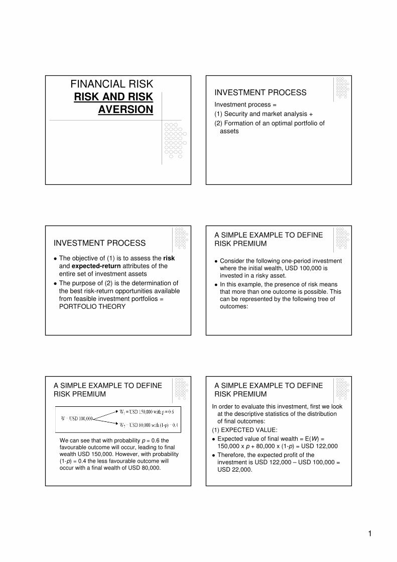
A SIMPLE EXAMPLE TO DEFINE RISK PREMIUM
� Consider the following one-period investment where the initial wealth, USD 100,000 is
invested in a risky asset.
� In this example, the presence of risk means that more than one outcome is possible. This can be represented by the following tree of
outcomes:
A SIMPLE EXAMPLE TO DEFINE RISK PREMIUM
We can see that with probability p = 0.6 the favourable outcome will occur, leading to final wealth USD 150,000. However, with probability
(1-p) = 0.4 the less favourable outcome will occur with a final wealth of USD 80,000.
A SIMPLE EXAMPLE TO DEFINE RISK PREMIUM
In order to evaluate this investment, first we look at the descriptive statistics of the distribution
of final outcomes:
(1) EXPECTED VALUE:
� Expected value of final wealth = E(W) =
150,000 x p + 80,000 x (1-p) = USD 122,000
� Therefore, the expected profit of the investment is USD 122,000 – USD 100,000 =
USD 22,000.
2
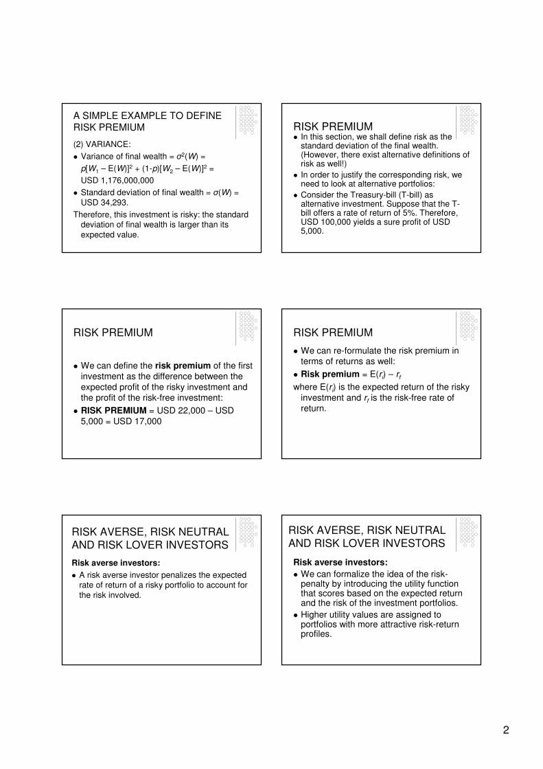
A SIMPLE EXAMPLE TO DEFINE RISK PREMIUM
(2) VARIANCE:
� Variance of final wealth = σ2(W) =
p[W1 – E(W)]2 + (1-p)[W2 – E(W)]2 =
USD 1,176,000,000
� Standard deviation of final wealth = σ(W) =
USD 34,293.
Therefore, this investment is risky: the standard deviation of final wealth is larger than its
expected value.
RISK PREMIUM� In this section, we shall define risk as the
standard deviation of the final wealth. (However, there exist alternative definitions of risk as well!)
� In order to justify the corresponding risk, we need to look at alternative portfolios:
� Consider the Treasury-bill (T-bill) as alternative investment. Suppose that the T-bill offers a rate of return of 5%. Therefore, USD 100,000 yields a sure profit of USD 5,000.
RISK PREMIUM
� We can define the risk premium of the first investment as the difference between the
expected profit of the risky investment and the profit of the risk-free investment:
� RISK PREMIUM = USD 22,000 – USD
5,000 = USD 17,000
RISK PREMIUM
� We can re-formulate the risk premium in terms of returns as well:
� Risk premium = E(ri) – rf
where E(ri) is the expected return of the risky
investment and rf is the risk-free rate of return.
RISK AVERSE, RISK NEUTRAL
AND RISK LOVER INVESTORS
Risk averse investors:
� A risk averse investor penalizes the expected rate of return of a risky portfolio to account for
the risk involved.
RISK AVERSE, RISK NEUTRAL
AND RISK LOVER INVESTORS
Risk averse investors:
� We can formalize the idea of the risk-penalty by introducing the utility function that scores based on the expected return and the risk of the investment portfolios.
� Higher utility values are assigned to portfolios with more attractive risk-return profiles.
3
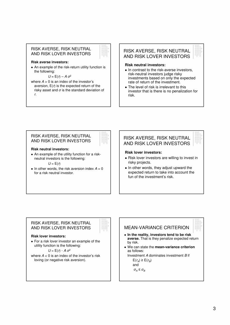
RISK AVERSE, RISK NEUTRAL AND RISK LOVER INVESTORS
Risk averse investors:
� An example of the risk-return utility function is
the following:
U = E(r) – A σ2
where A > 0 is an index of the investor’s aversion, E(r) is the expected return of the
risky asset and σ is the standard deviation of r.
Risk neutral investors:
� In contrast to the risk-averse investors, risk-neutral investors judge risky investments based on only the expected rate of return of the investment.
� The level of risk is irrelevant to this investor that is there is no penalization for risk.
RISK AVERSE, RISK NEUTRAL
AND RISK LOVER INVESTORS
RISK AVERSE, RISK NEUTRAL AND RISK LOVER INVESTORS
Risk neutral investors:
� An example of the utility function for a risk-
neutral investors is the following:
U = E(r)
� In other words, the risk aversion index A = 0 for a risk neutral investor.
Risk lover investors:
� Risk lover investors are willing to invest in
risky projects.
� In other words, they adjust upward the
expected return to take into account the fun of the investment’s risk.
RISK AVERSE, RISK NEUTRAL
AND RISK LOVER INVESTORS
RISK AVERSE, RISK NEUTRAL AND RISK LOVER INVESTORS
Risk lover investors:
� For a risk lover investor an example of the
utility function is the following:
U = E(r) - A σ2
where A < 0 is an index of the investor’s risk loving (or negative risk aversion).
MEAN-VARIANCE CRITERION
� In the reality, investors tend to be risk averse. That is they penalize expected return by risk.
� We can state the mean-variance criterionas follows:
Investment A dominates investment B if
E(rA) ≥ E(rB)
and
σA ≤ σB
4
MEAN-VARIANCE CRITERION
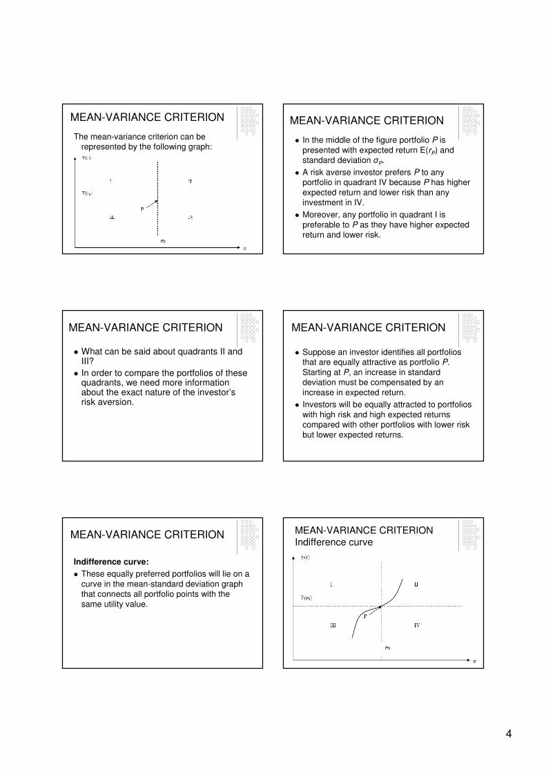
The mean-variance criterion can be represented by the following graph:
MEAN-VARIANCE CRITERION
� In the middle of the figure portfolio P is
presented with expected return E(rP) and standard deviation σP.
� A risk averse investor prefers P to any portfolio in quadrant IV because P has higher
expected return and lower risk than any investment in IV.
� Moreover, any portfolio in quadrant I is
preferable to P as they have higher expected return and lower risk.
MEAN-VARIANCE CRITERION
� What can be said about quadrants II and III?
� In order to compare the portfolios of these quadrants, we need more information about the exact nature of the investor’s risk aversion.
MEAN-VARIANCE CRITERION
� Suppose an investor identifies all portfolios that are equally attractive as portfolio P.
Starting at P, an increase in standard deviation must be compensated by an
increase in expected return.
� Investors will be equally attracted to portfolios
with high risk and high expected returns compared with other portfolios with lower risk
but lower expected returns.
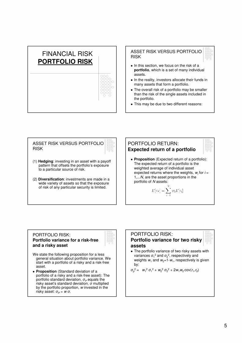
MEAN-VARIANCE CRITERION
Indifference curve:
� These equally preferred portfolios will lie on a
curve in the mean-standard deviation graph that connects all portfolio points with the
same utility value.
MEAN-VARIANCE CRITERION Indifference curve
5
FINANCIAL RISKPORTFOLIO RISK
ASSET RISK VERSUS PORTFOLIO RISK
� In this section, we focus on the risk of a portfolio, which is a set of many individual
assets.
� In the reality, investors allocate their funds in
many assets that form a portfolio.
� The overall risk of a portfolio may be smaller than the risk of the single assets included in
the portfolio.
� This may be due to two different reasons:
ASSET RISK VERSUS PORTFOLIO RISK
(1) Hedging: investing in an asset with a payoff pattern that offsets the portfolio’s exposure to a particular source of risk.
(2) Diversification: investments are made in a wide variety of assets so that the exposure of risk of any particular security is limited.
PORTFOLIO RETURN:
Expected return of a portfolio
� Proposition (Expected return of a portfolio): The expected return of a portfolio is the
weighted average of individual asset expected returns where the weights, wi for i =
1,...N, are the asset proportions in the portfolio of N assets:
PORTFOLIO RISK:
Portfolio variance for a risk-free and a risky asset
We state the following proposition for a less general situation about portfolio variance. We start with a portfolio of a risky and a risk-free asset.
� Proposition (Standard deviation of a portfolio of a risky and a risk-free asset): The portfolio standard deviation, σP equals the risky asset’s standard deviation, σ multiplied by the portfolio proportion, w invested in the risky asset: σP = w σ.
PORTFOLIO RISK: Portfolio variance for two risky assets� The portfolio variance of two risky assets with
variances σ12 and σ2
2, respectively and
weights w1 and w2=1-w1, respectively is given by:
σp2 = w1
2 σ12 + w2
2 σ22 + 2w1w2 cov(r1,r2)
6
EXAMPLE: Portfolio variance for two risky
assets
� Remark:
Covariance = cov(r1,r2) = σ1σ2ρ12
where -1 ≤ ρ12 ≤ 1 denotes the correlation coefficient.
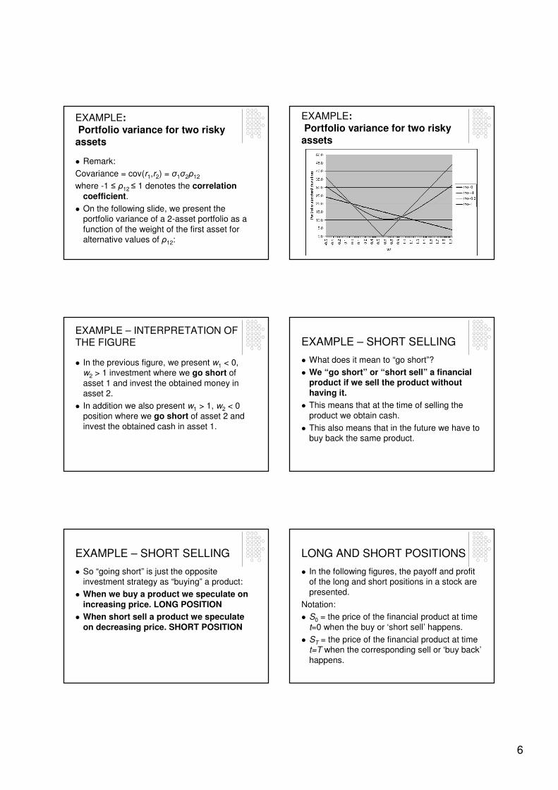
� On the following slide, we present the portfolio variance of a 2-asset portfolio as a
function of the weight of the first asset for alternative values of ρ12:
EXAMPLE: Portfolio variance for two risky
assets
EXAMPLE – INTERPRETATION OF THE FIGURE
� In the previous figure, we present w1 < 0, w2 > 1 investment where we go short of
asset 1 and invest the obtained money in asset 2.
� In addition we also present w1 > 1, w2 < 0 position where we go short of asset 2 and
invest the obtained cash in asset 1.
EXAMPLE – SHORT SELLING
� What does it mean to “go short”?
� We “go short” or “short sell” a financial product if we sell the product without having it.
� This means that at the time of selling the
product we obtain cash.
� This also means that in the future we have to buy back the same product.
EXAMPLE – SHORT SELLING
� So “going short” is just the opposite investment strategy as “buying” a product:
� When we buy a product we speculate on increasing price. LONG POSITION
� When short sell a product we speculate on decreasing price. SHORT POSITION
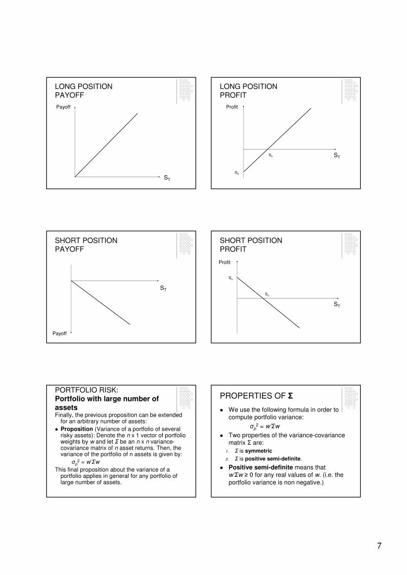
LONG AND SHORT POSITIONS
� In the following figures, the payoff and profit of the long and short positions in a stock are
presented.
Notation:
� S0 = the price of the financial product at time
t=0 when the buy or ‘short sell’ happens.
� ST = the price of the financial product at time t=T when the corresponding sell or ‘buy back’
happens.
7
LONG POSITIONPAYOFF
ST
Payoff
LONG POSITIONPROFIT
-S0
S0 ST
Profit
SHORT POSITION PAYOFF
Payoff
ST
SHORT POSITION PROFIT
Profit
ST
S0
S0
PORTFOLIO RISK: Portfolio with large number of assetsFinally, the previous proposition can be extended
for an arbitrary number of assets:
� Proposition (Variance of a portfolio of several risky assets): Denote the n x 1 vector of portfolio weights by w and let Σ be an n x n variance-covariance matrix of n asset returns. Then, the variance of the portfolio of n assets is given by:
σp2 = w’Σw
This final proposition about the variance of a portfolio applies in general for any portfolio of large number of assets.
PROPERTIES OF Σ
� We use the following formula in order to compute portfolio variance:
σp2 = w’Σw
� Two properties of the variance-covariance matrix Σ are:
1. Σ is symmetric
2. Σ is positive semi-definite.
� Positive semi-definite means that w’Σw ≥ 0 for any real values of w. (i.e. the
portfolio variance is non negative.)

8
HOW TO CHECK THAT Σ IS POSITIVE SEMI-DEFINITE?
� Therefore, when we choose the elements of Σ, we have to check if Σ is positive semi-
definite.
� The definiteness of a matrix can be checked by computing the determinant of the matrix.
� There is a function for this in Excel: MDETERM().
� Proposition. A matrix is positive semi-
definite if its determinant, D ≥ 0.
EXAMPLE:
Portfolio variance for three risky assets
� For example, let us consider the case of three assets:
� Doing simple algebra, from w’Σw we can
express the portfolio variance of three assets as follows:
σp2 = w1
2 σ12 + w2
2 σ22 + w3
2 σ32
+ 2w1w2cov(r1,r2) + 2w1w3cov(r1,r3)
+ 2w2w3cov(r2,r3)
9
VALUE AT RISK
DEFINITION OF RISK
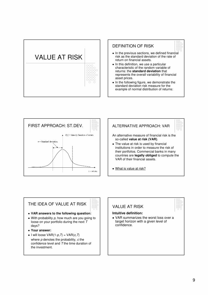
� In the previous sections, we defined financial risk as the standard deviation of the rate of return on financial assets.
� In this definition, we use a particular characteristic of the random variable of returns: the standard deviation that represents the overall variability of financial asset prices.
� In the following figure, we demonstrate the standard deviation risk measure for the example of normal distribution of returns:
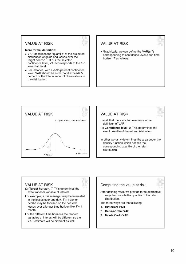
FIRST APPROACH: ST.DEV. ALTERNATIVE APPROACH: VAR
An alternative measure of financial risk is the so-called value at risk (VAR).
� The value at risk is used by financial institutions in order to measure the risk of
their portfolios. Commercial banks in many countries are legally obliged to compute the
VAR of their financial assets.
� What is value at risk?
THE IDEA OF VALUE AT RISK
� VAR answers to the following question:
� With probability p, how much are you going to loose on your portfolio during the next T
days?
� Your answer:
� I will loose VAR(1-p,T) = VAR(c,T)
where p denotes the probability, c the
confidence level and T the time duration of the investment.
VALUE AT RISK
Intuitive definition:
� VAR summarizes the worst loss over a target horizon with a given level of confidence.
10
VALUE AT RISK
More formal definition:
� VAR describes the “quantile” of the projected distribution of gains and losses over the target horizon T. If c is the selected confidence level, VAR corresponds to the 1-clower-tail level.
� For instance, with a c=95 percent confidence level, VAR should be such that it exceeds 5 percent of the total number of observations in the distribution.
VALUE AT RISK
� Graphically, we can define the VAR(c,T)
corresponding to confidence level c and time horizon T as follows:
VALUE AT RISK VALUE AT RISK
Recall that there are two elements in the definition of VAR:
(1) Confidence level, c: This determines the
exact quantile of the return distribution.
In other words, c determines the area under the
density function which defines the corresponding quantile of the return
distribution.
VALUE AT RISK(2) Target horizon, T: This determines the
exact random variable of interest.
For example, a risk manager may be interested
in the losses over one day, T = 1 day or he/she may be focused on the possible
losses over a longer time horizon like T = 1 month.
For the different time horizons the random variables of interest will be different so the
VAR estimate will be different as well.
Computing the value at risk
After defining VAR, we provide three alternative ways to compute the quantile of the return
distribution.
The three ways are the following:
1. Historical VAR
2. Delta-normal VAR
3. Monte Carlo VAR
11
HISTORICAL VAR
HISTORICAL VAR
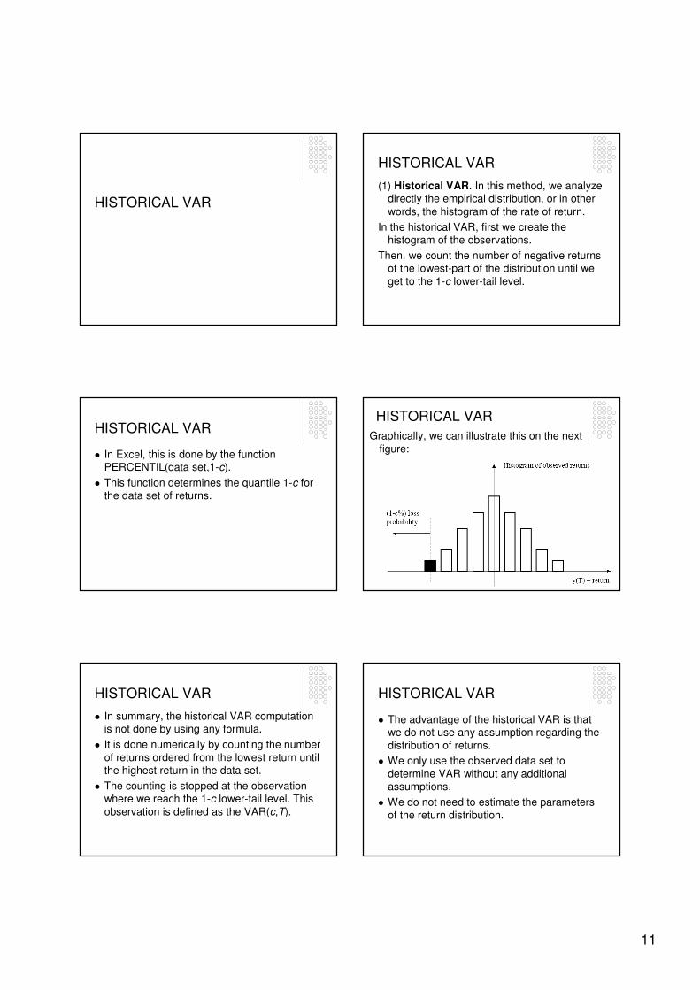
(1) Historical VAR. In this method, we analyze directly the empirical distribution, or in other
words, the histogram of the rate of return.
In the historical VAR, first we create the histogram of the observations.
Then, we count the number of negative returns of the lowest-part of the distribution until we
get to the 1-c lower-tail level.
HISTORICAL VAR
� In Excel, this is done by the function PERCENTIL(data set,1-c).
� This function determines the quantile 1-c for the data set of returns.
HISTORICAL VAR
Graphically, we can illustrate this on the next
figure:
HISTORICAL VAR
� In summary, the historical VAR computation is not done by using any formula.
� It is done numerically by counting the number
of returns ordered from the lowest return until the highest return in the data set.
� The counting is stopped at the observation where we reach the 1-c lower-tail level. This
observation is defined as the VAR(c,T).
HISTORICAL VAR
� The advantage of the historical VAR is that we do not use any assumption regarding the
distribution of returns.
� We only use the observed data set to
determine VAR without any additional assumptions.
� We do not need to estimate the parameters
of the return distribution.
12
HISTORICAL VAR
� The disadvantage of the historical VAR is that we only use past observations in order to
infer the future return distribution.
� The data set of past returns may be small
and/or non-representative for the inference of the 1-c quantile.
DELTA-NORMAL VAR
DELTA-NORMAL VAR
� We are in day t=0 (present) and we are interested in computing VAR of portfolio invested over a time horizon of T days.
� Denote the return of the investment by:
� y(T,0) is the return obtained between time t=0and time t=T. In the formula, T denotes the
time horizon of the investment.
DELTA-NORMAL VAR
� In this approach, we make an assumption about the distribution of asset returns
denoted:
� Assumption. The distribution of the rate of
return y(T,0) is a normal distribution:
� y(T,0) ~ N[µ(T),σ2(T)]
DELTA-NORMAL VAR
� This assumption allows us to obtain the following formula for VAR(c,T):
VAR(c,T) = µ(T) + σ(T) Z1-c
where Z1-c is the “quantile 1-c” of the standard normal distribution N(0,1).
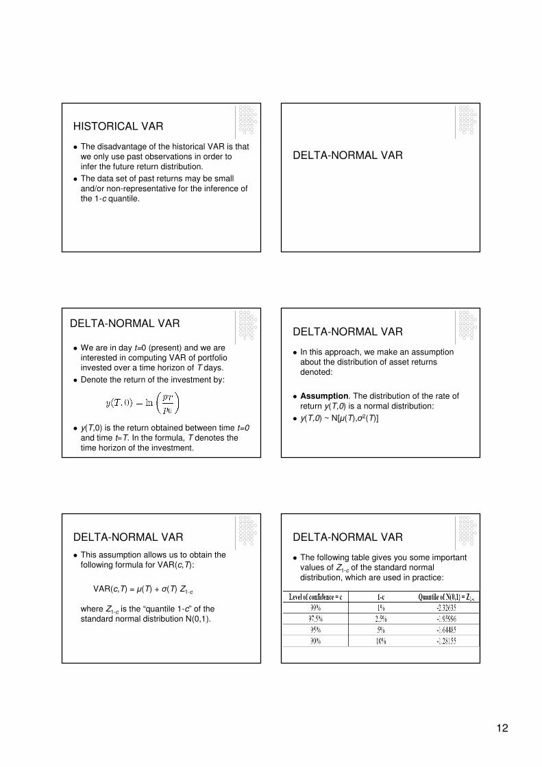
DELTA-NORMAL VAR
� The following table gives you some important values of Z1-c of the standard normal
distribution, which are used in practice:
13
DELTA-NORMAL VAR
� The main advantage of the delta-normal VAR is that it is computationally easy to get
the VAR estimate:
� We only have to substitute the parameters
µ(T), σ(T) and Z1-c into the formula and compute the VAR(c,T).
DELTA-NORMAL VAR
� The disadvantage of the delta-normal VAR is that we need to estimate µ(T) and σ(T)
using past returns with time horizon T.
� (1) Thus, the delta-normal VAR also uses
historical data to estimate the parameters.
� (2) The estimation of µ(T) and σ(T) requires a large data set of y(T,0) that may not be
available.
DELTA-NORMAL VARExample:
� Imagine that we want to compute 30-days delta-normal VAR.
� For this, we need to estimate µ(T) and σ(T)
using a sample of 120 observations of the past.
� This means a 120 x 30-days time span,
which is approximately 10 years of past data.
� This may not be available or irrelevant for us.
DELTA-NORMAL VAR
� In practice, it may happen that the time horizon of the returns for which we have
sufficient sample size is different from the time horizon of the VAR(c,T).
� In particular, it is possible that we observe daily returns
y(t,t-1) for t=1,2,3,...,T
but we need to compute VAR(c,T) for a
longer time horizon.
DELTA-NORMAL VAR
� On the following slides, we derive an explicit formula of VAR(c,T) for the case when y(t,t-1)
daily returns are observed.
� We proceed in two steps:
� Step (1): Show that the log returns are
additive.
� Step (2): Assume that y(t,t-1) returns are independent and identically distributed
random variables with normal distribution.
DELTA-NORMAL VARStep (1): Log returns are additive
Consider 2 consecutive 1-day returns:
� y(t,t-1) = ln(pt/pt-1) = lnpt – lnpt-1
� y(t+1,t) = ln(pt+1/pt) = lnpt+1 – lnpt
� The first equality in each equation is based
on the definition of log return.
� The second equality in each equation is
based on a property of the logarithm.
14
DELTA-NORMAL VARStep (1): Log returns are additive
� From two consecutive daily returns, we
can obtain the return for the two-day period (t+1,t-1) as the sum of two
consecutive daily returns:
y(t+1,t-1) = lnpt+1 – lnpt-1 =
lnpt+1 – lnpt-1 + (lnpt – lnpt) =
(lnpt+1 – lnpt) + (lnpt – lnpt-1) =
y(t+1,t) + y(t,t-1)
DELTA-NORMAL VARStep (1): Log returns are additive
� Notice that this additive property is not true for the ‘traditional’ definition of return:
y(t,t-1) = (pt-pt-1)/pt-1
� This is one of the reasons why in finance the log return formula is frequently used.
DELTA-NORMAL VAR
Step (1): Log returns are additive
� The consequence is that daily logarithmic returns are additive:
� We can compute the return for a longer T-day time horizon by adding the
consecutive one-period returns between day t=0 and day t=T:
DELTA-NORMAL VARStep (2): Assumption of independence
� Suppose that daily returns y(t,t-1) ~ N[µ(1),σ2(1)] for t=1,2,3,...
are independent and identically distributed
(denoted i.i.d.).
� Independence means that return of day t is not influenced by the returns of other days.
� Identical distribution means that all returns y(1,0), y(2,1), y(3,2), ... have to same
distribution.
DELTA-NORMAL VAR
� From steps 1 and 2, it follows that y(T,0) is also normally distributed with the next
parameters
y(T,0) ~ N[µ(T),σ2(T)] = N[Tµ(1),Tσ2(1)]
� The second equality follows from steps 1 and 2.
DELTA-NORMAL VAR
� Given that we have a large data set on daily returns, we can estimate properly
µ(1) and σ(1).
� Then, we can compute the estimates of
µ(T) and σ(T) by
� µ(T)=Tµ(1) and σ(T)=
15
DELTA-NORMAL VAR
� Substituting these parameters into the first delta-normal VAR formula, we get:
DELTA-NORMAL VAR
Summary:
� It is not necessary to have data on the T time
horizon returns.
� It is enough to observe the daily returns y(t,t-1) and estimate the parameters of the
y(t,t-1) ~ N[µ(1),σ2(1)] distribution.
� Then, we can substitute the estimated parameters into the formula presented on the previous slide to get the VAR.
MONTE-CARLO VAR
MONTE CARLO (MC) VAR
� The final method of VAR computation is based on Monte Carlo simulation of future
returns.
� In this method, as in the delta-normal VAR, we need to assume the distribution of returns.
� Then, we have to simulate a large number of returns each interpreted as one possible
realization of the future return over the time horizon we are interested in.
MONTE CARLO (MC) VAR� For example, suppose that we need the
compute the 1-day VAR(c,1) using MC method to estimate the largest possible loss during tomorrow.
� To do this, we simulate thousands of
realizations from y(1,0).
� Each of these simulations is interpreted as a possible return of tomorrow.
MONTE CARLO (MC) VAR
� After simulating a large number of realizations of the return, we determine
numerically the VAR using the same procedure what we did for the historicalVAR computation.
� Thus, in Excel, we use again the function
PERCENTIL(data set,1-c).
16
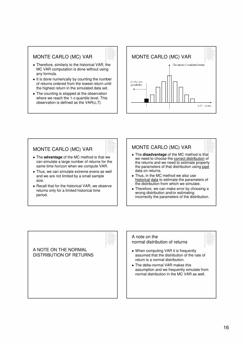
MONTE CARLO (MC) VAR
� Therefore, similarly to the historical VAR, the MC VAR computation is done without using
any formula.
� It is done numerically by counting the number of returns ordered from the lowest return until the highest return in the simulated data set.
� The counting is stopped at the observation
where we reach the 1-c quantile level. This observation is defined as the VAR(c,T).
MONTE CARLO (MC) VAR
MONTE CARLO (MC) VAR
� The advantage of the MC method is that we can simulate a large number of returns for the
same time horizon when we compute VAR.
� Thus, we can simulate extreme evens as well and we are not limited by a small sample size.
� Recall that for the historical VAR, we observe
returns only for a limited historical time period.
MONTE CARLO (MC) VAR
� The disadvantage of the MC method is that we need to choose the correct distribution of the returns and we need to estimate properly the parameters of that distribution using pastdata on returns.
� Thus, in the MC method we also use historical data to estimate the parameters of the distribution from which we simulate.
� Therefore, we can make error by choosing a wrong distribution and/or estimating incorrectly the parameters of the distribution.
A NOTE ON THE NORMAL
DISTRIBUTION OF RETURNS
A note on the normal distribution of returns
� When computing VAR it is frequently assumed that the distribution of the rate of
return is a normal distribution.
� The delta-normal VAR makes this
assumption and we frequently simulate from normal distribution in the MC VAR as well.
17
A note on the normal distribution of returns
The main reasons of the assumption of
normality is computational convenience.
A note on the normal distribution of returns
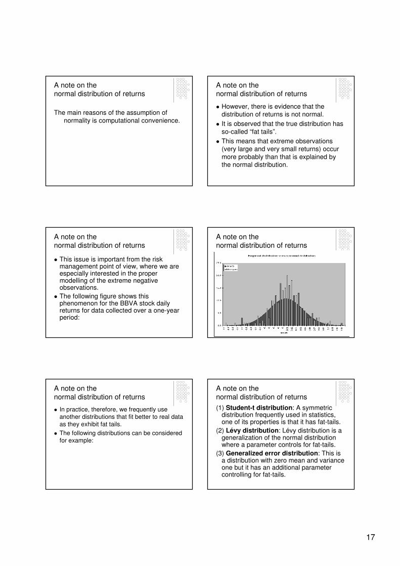
� However, there is evidence that the distribution of returns is not normal.
� It is observed that the true distribution has
so-called “fat tails”.
� This means that extreme observations (very large and very small returns) occur
more probably than that is explained by the normal distribution.
A note on the normal distribution of returns
� This issue is important from the risk management point of view, where we are especially interested in the proper modelling of the extreme negative observations.
� The following figure shows this phenomenon for the BBVA stock daily returns for data collected over a one-year period:
A note on the normal distribution of returns
A note on the normal distribution of returns
� In practice, therefore, we frequently use another distributions that fit better to real data
as they exhibit fat tails.
� The following distributions can be considered for example:
A note on the normal distribution of returns
(1) Student-t distribution: A symmetric distribution frequently used in statistics, one of its properties is that it has fat-tails.
(2) Lévy distribution: Lévy distribution is a generalization of the normal distribution where a parameter controls for fat-tails.
(3) Generalized error distribution: This is a distribution with zero mean and variance one but it has an additional parameter controlling for fat-tails.
18
ALTERNATIVE APPROACHES TO
MODEL VOLATILITY
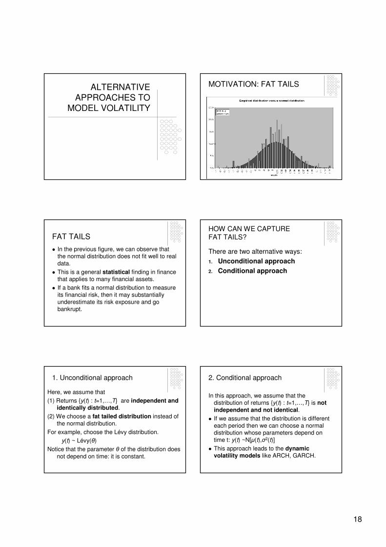
MOTIVATION: FAT TAILS
FAT TAILS
� In the previous figure, we can observe that the normal distribution does not fit well to real
data.
� This is a general statistical finding in finance that applies to many financial assets.
� If a bank fits a normal distribution to measure its financial risk, then it may substantially
underestimate its risk exposure and go bankrupt.
HOW CAN WE CAPTURE FAT TAILS?
There are two alternative ways:
1. Unconditional approach
2. Conditional approach
1. Unconditional approach
Here, we assume that
(1) Returns {y(t) : t=1,…,T} are independent and identically distributed.
(2) We choose a fat tailed distribution instead of
the normal distribution.
For example, choose the Lévy distribution.
y(t) ~ Lévy(θ)
Notice that the parameter θ of the distribution does
not depend on time: it is constant.
2. Conditional approach
In this approach, we assume that the distribution of returns {y(t) : t=1,…,T} is not independent and not identical.
� If we assume that the distribution is different each period then we can choose a normal distribution whose parameters depend on
time t: y(t) ~N[µ(t),σ2(t)]
� This approach leads to the dynamic volatility models like ARCH, GARCH.
19
DYNAMIC MODELS OF VOLATILITY
MOTIVATION� Both in the theory and practice of finance,
volatility modelling is important.
� Volatility estimates are used for:
(1) Risk management purposes (for example to
compute the VAR of a portfolio).
(2) Financial asset valuation purposes (for
example to determine to fair price of derivatives contracts).
(3) Portfolio construction purposes (we need volatility estimates in order to construct the
optimal risk-return portfolio).
VOLATILITY
� In this section, volatility is defined as the
standard deviation of asset returns.
CONTSTANT VOLATILITY
� In the previous sections, we modelled the standard deviation of returns and volatility was assumed to be constant over time.
� We also assumed in the model construction that daily returns were independent random variables.
CHANGING VOLATILITY
� Nevertheless, in practice these assumptions are not valid.
� There is empirical evidence that the time series of returns is not an independent
sequence of random variables.
DYNAMIC VOLATILITY MODEL
� In particular, there is evidence that the volatility of returns, σt with t=1,...,T form a
serially correlated time series.
� Therefore, returns are not independent.
� This phenomenon can be modelled by a so-
called dynamic volatility model.
20
DYNAMIC VOLATILITY MODELS
We are going to present various models of dynamic volatility:
1. GARCH-type models
(a) ARCH,
(b) GARCH,
(c) EGARCH
2. Stochastic volatility models
1(a) ARCH MODEL
GARCH-type volatility modelsARCH
� The ARCH model has been developed by Robert Engle (1982, Econometrica) and
became very popular for the dynamic modelling of volatility.
� ARCH = autoregressive conditional heteroscedasticity
GARCH-type volatility modelsARCH
� The ARCH(1) model is frequently used:
� where αi>0 for i=1,0 to ensure positive value
of volatility.
� The ht denotes the variance of yt.
GARCH-type volatility modelsARCH
� The ARCH(q) model is formulated as follows:
� where αi>0 for i=1,...,q to ensure positive value of volatility.
� The ht denotes the variance of yt.
GARCH-type volatility modelsARCH
Stationarity:
� When a dynamic volatility model is estimated, it is important to check if the
parameters estimates of the model determine a stationary or a non-stationary
time series of volatility.
21
GARCH-type volatility modelsARCH
Stationarity:
� The ARCH(q) model is stationary if
� The ARCH(1) model is stationary if α1<1.
1(b) GARCH MODEL
GARCH-type volatility modelsGARCH
� After the success of the ARCH model several extensions have been proposed by
researchers.
� Probably the most popular extension is the
GARCH(p,q) introduced by Bollerslev (1986).
GARCH-type volatility modelsGARCH
� GARCH = generalized autoregressive conditional heteroscedasticity
� The GARCH model is probably the most used dynamic volatility model in practice.
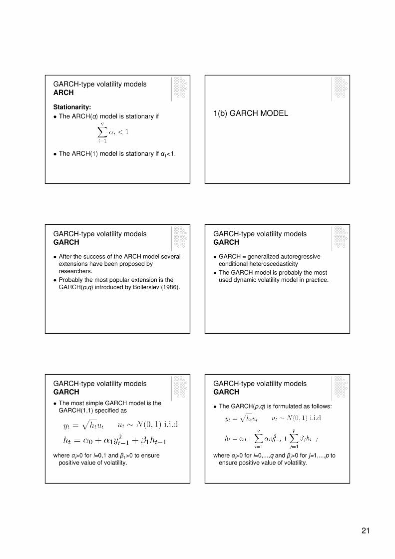
GARCH-type volatility modelsGARCH
� The most simple GARCH model is the GARCH(1,1) specified as
where αi>0 for i=0,1 and β1>0 to ensure positive value of volatility.
GARCH-type volatility modelsGARCH
� The GARCH(p,q) is formulated as follows:
where αi>0 for i=0,...,q and βj>0 for j=1,...,p to ensure positive value of volatility.
22
GARCH-type volatility modelsGARCH
Stationarity:
� The GARCH(1,1) model is stationary if
α1+β1<1.
� The GARCH(p,q) model is stationary if
1(c) EGARCH MODEL
GARCH-type volatility modelsEGARCH
� A further modification of the GARCH model is the exponential-GARCH or EGARCH
developed by Nelson (1991, Econometrica).
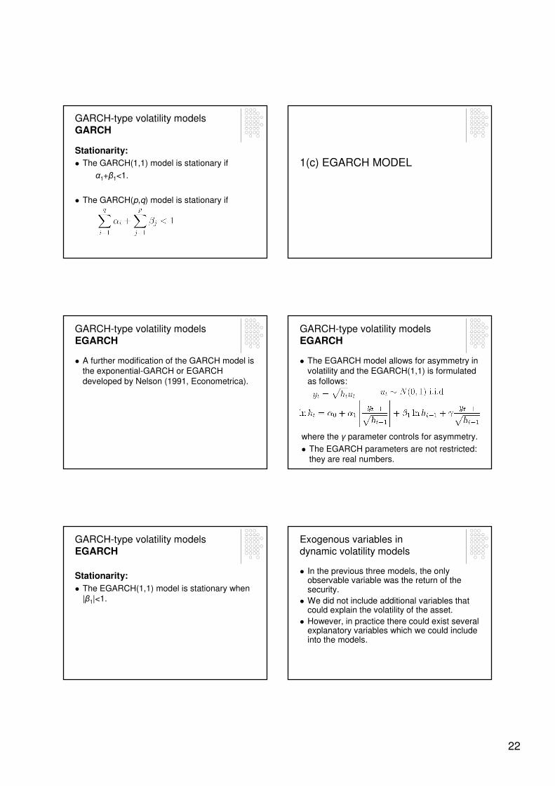
GARCH-type volatility modelsEGARCH
� The EGARCH model allows for asymmetry in volatility and the EGARCH(1,1) is formulated
as follows:
where the γ parameter controls for asymmetry.
� The EGARCH parameters are not restricted: they are real numbers.
GARCH-type volatility modelsEGARCH
Stationarity:
� The EGARCH(1,1) model is stationary when |β1|<1.
Exogenous variables in dynamic volatility models
� In the previous three models, the only observable variable was the return of the security.
� We did not include additional variables that could explain the volatility of the asset.
� However, in practice there could exist several explanatory variables which we could include into the models.
23
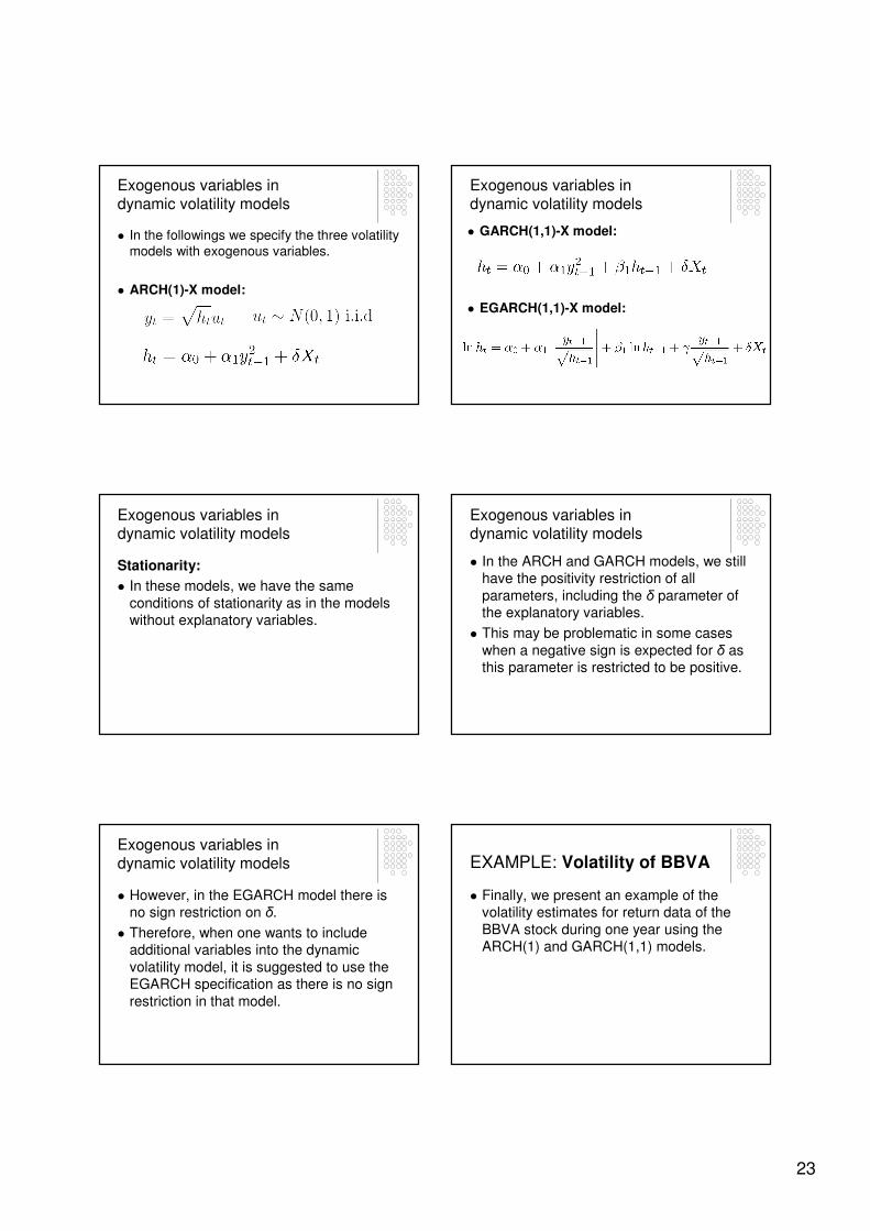
Exogenous variables in dynamic volatility models
� In the followings we specify the three volatility models with exogenous variables.
� ARCH(1)-X model:
Exogenous variables in dynamic volatility models
� GARCH(1,1)-X model:
� EGARCH(1,1)-X model:
Exogenous variables in dynamic volatility models
Stationarity:
� In these models, we have the same
conditions of stationarity as in the models without explanatory variables.
Exogenous variables in dynamic volatility models
� In the ARCH and GARCH models, we still have the positivity restriction of all
parameters, including the δ parameter of the explanatory variables.
� This may be problematic in some cases
when a negative sign is expected for δ as this parameter is restricted to be positive.
Exogenous variables in dynamic volatility models
� However, in the EGARCH model there is no sign restriction on δ.
� Therefore, when one wants to include additional variables into the dynamic
volatility model, it is suggested to use the EGARCH specification as there is no sign
restriction in that model.
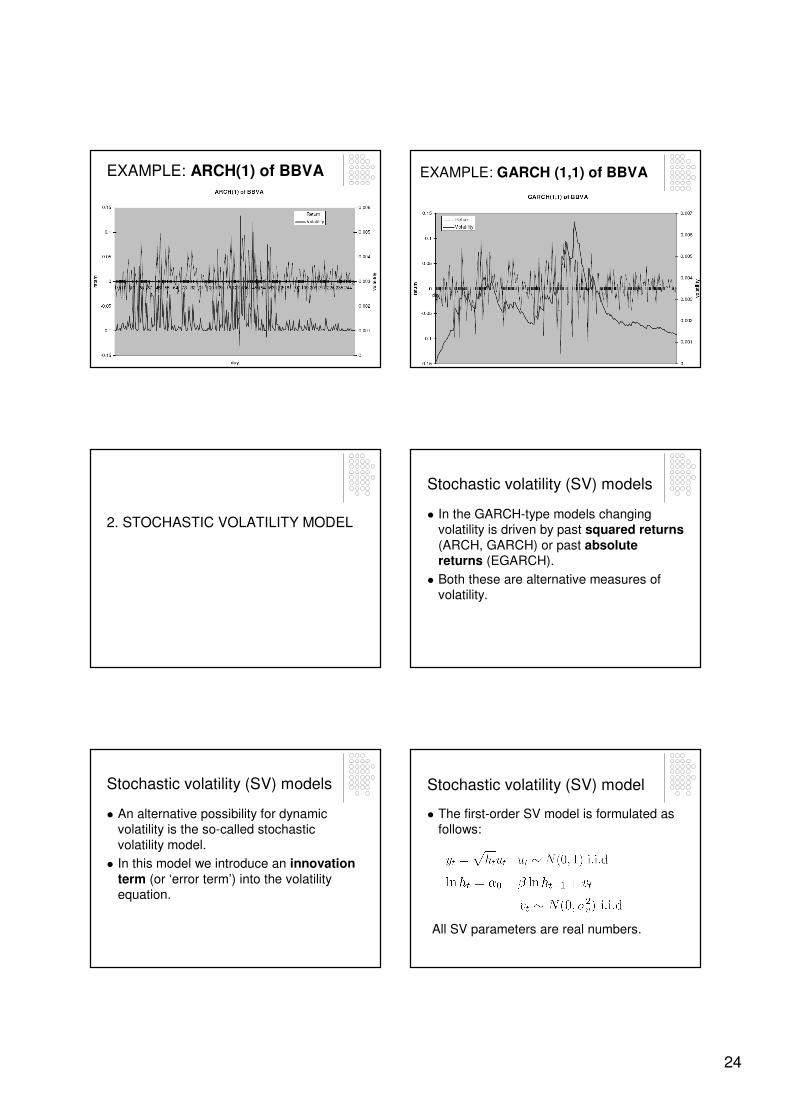
EXAMPLE: Volatility of BBVA
� Finally, we present an example of the volatility estimates for return data of the
BBVA stock during one year using the ARCH(1) and GARCH(1,1) models.
24
EXAMPLE: ARCH(1) of BBVA EXAMPLE: GARCH (1,1) of BBVA
2. STOCHASTIC VOLATILITY MODEL
Stochastic volatility (SV) models
� In the GARCH-type models changing volatility is driven by past squared returns(ARCH, GARCH) or past absolute returns (EGARCH).
� Both these are alternative measures of volatility.
Stochastic volatility (SV) models
� An alternative possibility for dynamic volatility is the so-called stochastic
volatility model.
� In this model we introduce an innovation term (or ‘error term’) into the volatility equation.
Stochastic volatility (SV) model
� The first-order SV model is formulated as follows:
All SV parameters are real numbers.

25
Stochastic volatility (SV) model
Stationarity
� The first-order SV model is stationary when |β|<1.
� The model can be easily extended to include more lags of volatility.

26
FORECASTING SECURITY PRICES
STRUCTURE OF CLASS
1. Motivation
2. Definition of forecast
3. Procedure of forecasting
4. Econometric models used for forecasting
STRUCTURE OF CLASS
5. Evaluation of forecast precision
6. Out-of-sample and
in-the-sample forecasting
7. One-step-ahead and Multi-step-ahead forecasts
MOTIVATION
� Investors and financial analysts are frequently interested in forecasting prices of
financial assets.
� Bank analysts frequently write reports to their clients about expected prices of financial products.
OUR APPROACH
OUR APPROACH
� In this class, we are interested in the direction of the price change.
� We model the log return on the investment at
time t:
yt = ln(pt/pt-1)
27
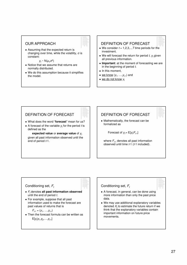
OUR APPROACH
� Assuming that the expected return is changing over time, while the volatility, σ is
constant:
yt ~ N(µt,σ2)
� Notice that we assume that returns are
normally distributed.
� We do this assumption because it simplifies the model.
DEFINITION OF FORECAST� We consider t = 1,2,3,..,T time periods for the
investment.
� We will forecast the return for period t, yt given
all previous information.
� Important: at the moment of forecasting we are in the beginning of period t.
� In this moment,
� we know (y1, …,yt-1) and
� we do not know yt
DEFINITION OF FORECAST
� What does the word “forecast” mean for us?
� A forecast of the variable yt for the period t is
defined as the
expected value or average value of yt
given all past information observed until the end of period t-1.
DEFINITION OF FORECAST
� Mathematically, the forecast can be formalized as
Forecast of yt = E[yt|Ft-1]
where Ft-1 denotes all past information observed until time t-1 (t-1 included).
Conditioning set, Ft
� Ft denotes all past information observeduntil the end of period t.
� For example, suppose that all past
information used to make the forecast are past values of returns that is
Ft-1 = (y1, …,yt-1)
� Then the forecast formula can be written as
E[yt|y1,y2,…,yt-1]
Conditioning set, Ft
� A forecast, in general, can be done using more information than only the past price
data.
� We may use additional explanatory variables denoted Xt to estimate the future return if we think that the explanatory variables contain
important information on future price movements.
28
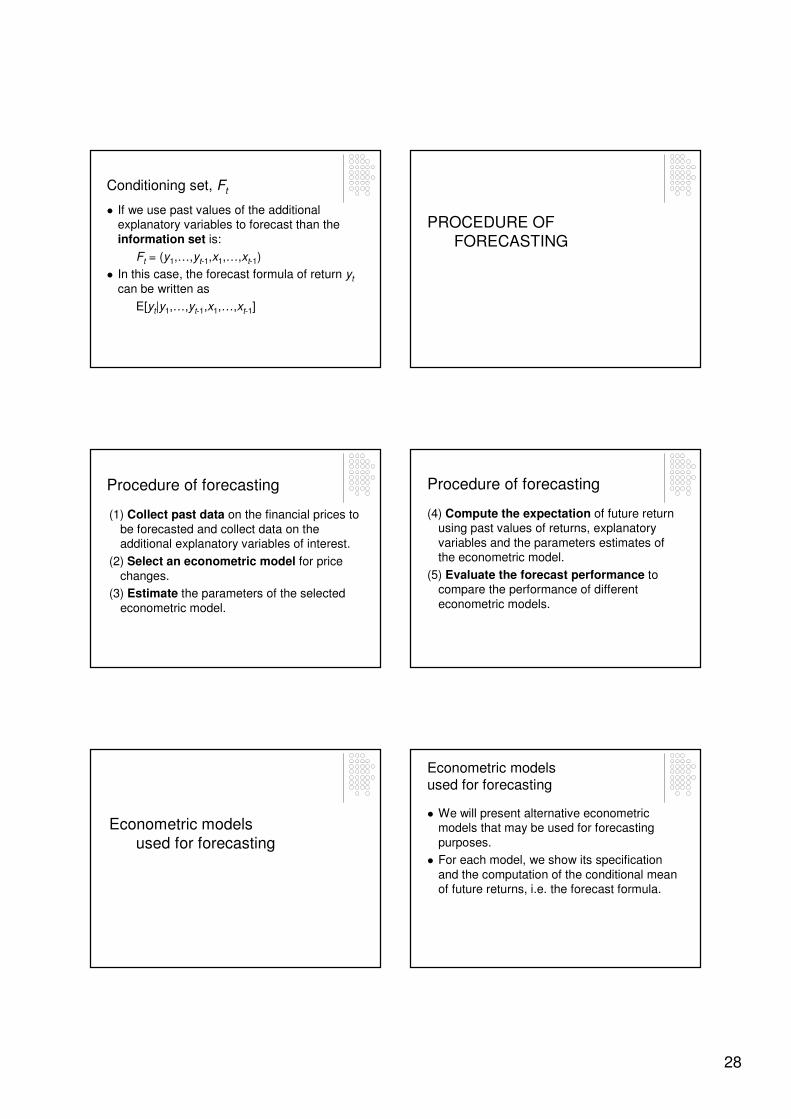
Conditioning set, Ft
� If we use past values of the additional explanatory variables to forecast than the
information set is:
Ft = (y1,…,yt-1,x1,…,xt-1)
� In this case, the forecast formula of return yt
can be written as
E[yt|y1,…,yt-1,x1,…,xt-1]
PROCEDURE OF
FORECASTING
Procedure of forecasting
(1) Collect past data on the financial prices to
be forecasted and collect data on the additional explanatory variables of interest.
(2) Select an econometric model for price
changes.
(3) Estimate the parameters of the selected
econometric model.
Procedure of forecasting
(4) Compute the expectation of future return using past values of returns, explanatory
variables and the parameters estimates of the econometric model.
(5) Evaluate the forecast performance to compare the performance of different
econometric models.
Econometric models
used for forecasting
Econometric models used for forecasting
� We will present alternative econometric models that may be used for forecasting
purposes.
� For each model, we show its specification
and the computation of the conditional mean of future returns, i.e. the forecast formula.

29
Econometric models used for forecasting
� We are going to present very general models that may include several lags of the variables.
� However, including many variables have two opposite effects on forecast precision:
Econometric models used for forecasting
(1) More variables mean more past information
used to forecast.
This is a POSITIVE effect.
Econometric models used for forecasting
(2) More variables mean more parameters to be estimated.
� This reduces the precision of the statistical
estimation of the model. (This means that the estimated parameter value may be far from the true value.)
This is NEGATIVE effect.
� In practice, we need to find the correct
balance between these two effects.
Econometric models used for forecasting
� We review various econometric models of the conditional mean of yt.
� In each model, we suppose that the volatility of the security is constant and that
the return is normally distributed:
yt ~ N(µt,σ2)
MODELS OF CONDITIONAL MEAN
� We suggest the following models for the
conditional mean:
1. AR(p)
2. ARMA(p,q)
3. AR(p)-X(k)
4. ARMA(p,q)-X(k)
AR(p) = autoregressive of order p
ARMA(p,q) = autoregressive (AR) of order pand moving average (MA) of order q
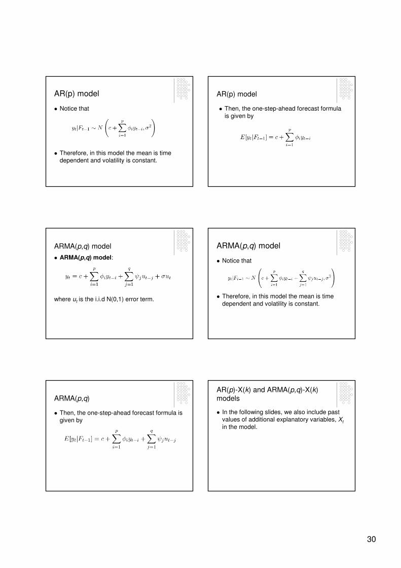
AR(p) model
� AR(p) model:
where ut is the i.i.d N(0,1) error term.
30
AR(p) model
� Notice that
� Therefore, in this model the mean is time dependent and volatility is constant.
AR(p) model
� Then, the one-step-ahead forecast formula is given by
ARMA(p,q) model
where ut is the i.i.d N(0,1) error term.
� ARMA(p,q) model:
ARMA(p,q) model
� Notice that
� Therefore, in this model the mean is time
dependent and volatility is constant.
ARMA(p,q)
� Then, the one-step-ahead forecast formula is given by
AR(p)-X(k) and ARMA(p,q)-X(k) models
� In the following slides, we also include past values of additional explanatory variables, Xt
in the model.
31
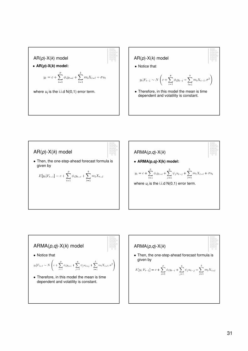
AR(p)-X(k) model
where ut is the i.i.d N(0,1) error term.
� AR(p)-X(k) model:
AR(p)-X(k) model
� Notice that
� Therefore, in this model the mean is time dependent and volatility is constant.
AR(p)-X(k) model
� Then, the one-step-ahead forecast formula is given by
ARMA(p,q)-X(k)
� ARMA(p,q)-X(k) model:
where ut is the i.i.d N(0,1) error term.
ARMA(p,q)-X(k) model
� Notice that
� Therefore, in this model the mean is time
dependent and volatility is constant.
ARMA(p,q)-X(k)
� Then, the one-step-ahead forecast formula is given by
32
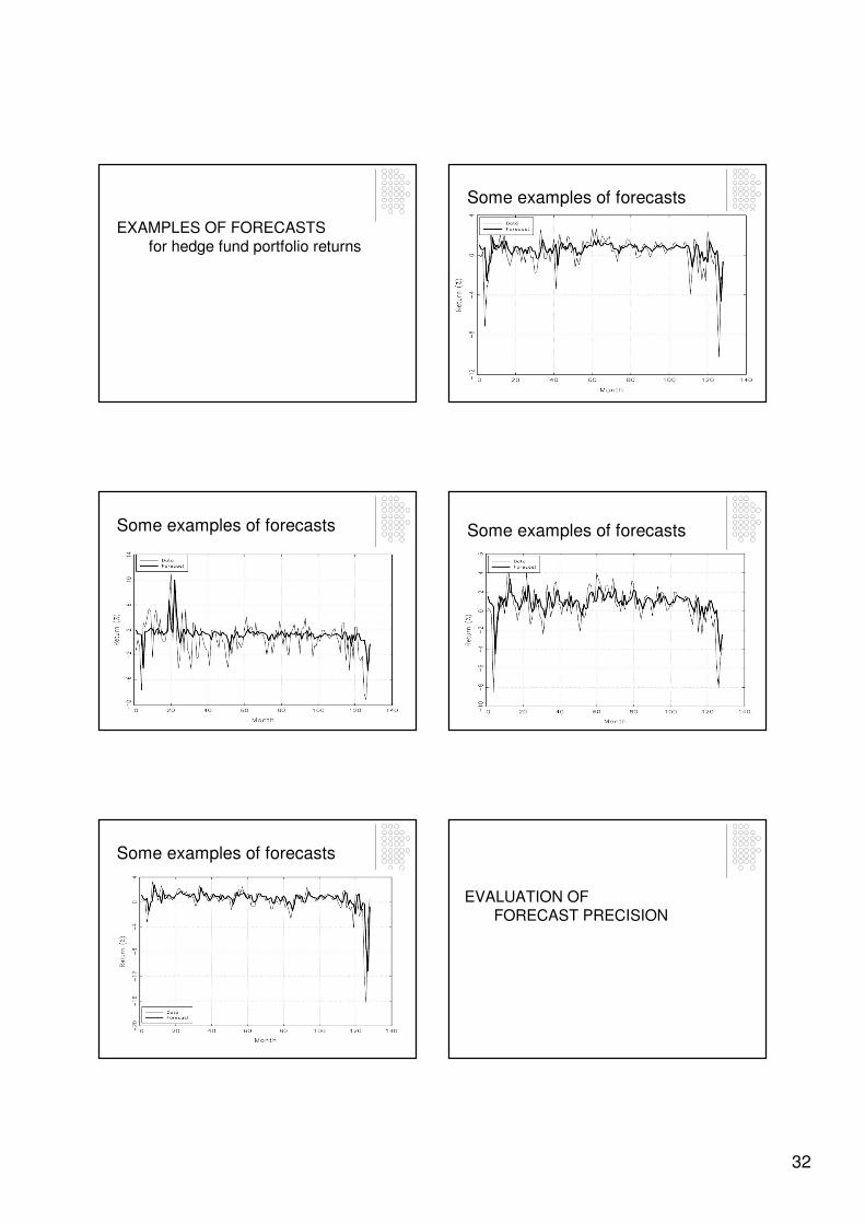
EXAMPLES OF FORECASTS
for hedge fund portfolio returns
Some examples of forecasts
Some examples of forecasts Some examples of forecasts
Some examples of forecasts
EVALUATION OF
FORECAST PRECISION

33
Evaluation of forecast precision
� Several alternative measures of forecast precision exist.
� These measures compare the distance of the true time series and the forecasted time
series.
� We present three alternative forecast performance measures:
(1) Mean absolute error (MAE),
(2) Mean square error (MSE) and
(3) Root mean square error (RMSE).
Evaluation of forecast precision
� The MAE, MSE and RMSE measures are formalized as follows:
where Yt-1 = (y1,y2,…,yt-1)
Evaluation of forecast precision
� An advantage of the MAE and RMSE measures is that the scale of both measures
is the same as the scale of the variable of interest that is forecasted, yt.
� The disadvantage of the MSE measure is that the scale of the MSE is different to the
scale of yt.
Out-of-sample and
in-the-sample forecasting
Out-of-sample and in-the-sample forecasting
� There are two ways to perform forecasting:
1. In-the-sample forecast
2. Out-of-sample forecast
In-the-sample forecast
� Suppose that we observe t = 1,…,T periods of returns.
� In the in-the-sample forecast, we estimate
an econometric model using data covering the period t = 1,…,T.
� Then, we “forecast” returns (already
observed) inside the t = 1,…,T period.
� This forecast procedure is not too realistic as
we use “future” information to estimate to parameters of the econometric model.

34
Out-of-sample forecast
� Suppose that we observe t = 1,…,T.
� In the out-of-sample forecast, we estimate an econometric model using data for the
period t = 1,…,T.
� Then, we forecast the return for next period t = T+1.
� This forecast procedure is more realistic as here we use only “past” information to
estimate the parameters of the econometric model.
One-step-ahead and Multi-step-ahead forecasts
One-step-ahead forecasts
� In the previous slides, we presented formulas for the one-step-ahead forecasts:
E[yt+1|y1,y2,…,yt]
� In the one-step-ahead forecast, we are only interested in the forecast of the next period
t+1 and we are not interested in forecasting further periods t+2, t+3,…
Multi-step-ahead forecasts
� However, in some situations it may be interesting to forecast for further periods.
� For example, we may need estimates of:
E[yt+2|y1,y2,…,yt]
E[yt+3|y1,y2,…,yt]
� These forecasts are called multi-step-ahead forecasts.
� In the example, these are two-step-ahead and three-step-ahead forecasts.

35
PORTFOLIO THEORY
THE MARKOWITZ PORTFOLIO SELECTION MODEL
� The portfolio selection models to be presented was developed by Harry Markowitz
in the 1950s.
PORTFOLIO THEORY
� Portfolio managers seek to achieve the best possible trade-off between risk and return.
� Suppose that the manager has to choose an
optimal combination of several risky assets and one risk-free asset.
� We structure the portfolio manager’s decision problem into to following two steps:
STEPS OF PORTFOLIO DECISION PROBLEM
STEP 1: Construct the optimal risky portfoliofrom the risky assets.
(1a) Asset allocation decision: the choice
about the distribution of the risky asset classes (stocks, bonds, real estate, foreign assets, etc.).
(1b) Security selection decision: the choice
of which particular securities to hold within each asset class.
STEPS OF PORTFOLIO DECISION PROBLEM
STEP 2: Construct the optimal complete portfolio from the optimal risky portfolio and
the risk-free asset.
(2) Capital allocation decision: the choice of
the proportion of the risk-free and the optimal risky portfolio.
STEP 1:
OPTIMAL RISKY PORTFOLIO
36
DIVERSIFICATION
� We begin with the discussion at a general level.
� We present how diversification can reduce the variance (or risk) of portfolio returns.
� Diversification means the inclusion of additional risky assets into the original risky portfolio.
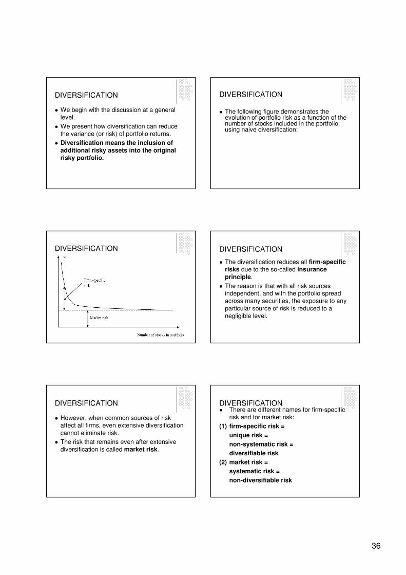
DIVERSIFICATION
� The following figure demonstrates the evolution of portfolio risk as a function of the number of stocks included in the portfolio using naive diversification:
DIVERSIFICATION DIVERSIFICATION
� The diversification reduces all firm-specific risks due to the so-called insurance principle.
� The reason is that with all risk sources independent, and with the portfolio spread across many securities, the exposure to any
particular source of risk is reduced to a negligible level.
DIVERSIFICATION
� However, when common sources of risk affect all firms, even extensive diversification
cannot eliminate risk.
� The risk that remains even after extensive
diversification is called market risk.
DIVERSIFICATION� There are different names for firm-specific
risk and for market risk:
(1) firm-specific risk =
unique risk =
non-systematic risk =
diversifiable risk
(2) market risk =
systematic risk =
non-diversifiable risk
37
PORTFOLIOS OF TWO RISKY
ASSETS
� In the following part of this section, we construct risky portfolios that provide the
lowest possible risk for any given level of expected return.
� We prove how diversification may reduce the variance of the portfolio of two risky assetscompared to the two individual risky assets on their own.
PORTFOLIOS OF TWO RISKY ASSETS
� Let the sub-index 1 denote the first and 2
denote the second risky asset. The portfolio variance is given by
σp2 = w1
2 σ12 + w2
2 σ22 + 2w1w2 σ1 σ2 ρ
where ρ denotes the correlation coefficient of
returns between the two risky assets.
PORTFOLIOS OF TWO RISKY ASSETS
� First, suppose that the two assets are perfectly correlated that is ρ = 1. Then, we
can simply derive that
σp = w1 σ1 + w2 σ2
� This means that when the assets are
perfectly correlated then the risk of the portfolio is simply the weighted average of
the individual standard deviations.
PORTFOLIOS OF TWO RISKY
ASSETS
� This also means that whenever ρ < 1, the
portfolios of risky assets offer better risk-return opportunities than the individual
component securities on their own.
PORTFOLIOS OF TWO RISKY
ASSETS
Minimum variance portfolio
Question:
� As w1 and w2=(1-w1) influence the portfolio variance, the investor would be interested in
the question of which value of weight w1
minimizes the risk of the portfolio for given
σ1, σ2 and ρ values?
PORTFOLIOS OF TWO RISKY
ASSETS
� We have to solve the following minimization
problem:
38
PORTFOLIOS OF TWO RISKY ASSETS
� Take derivative with respect to w1 and equal
zero the derivative:
PORTFOLIOS OF TWO RISKY ASSETS� Solve this equation for w1:
where cov(r1,r2) = σ1 σ2 ρ and
The portfolio with weights w1* and w2* define the minimum variance portfolio.
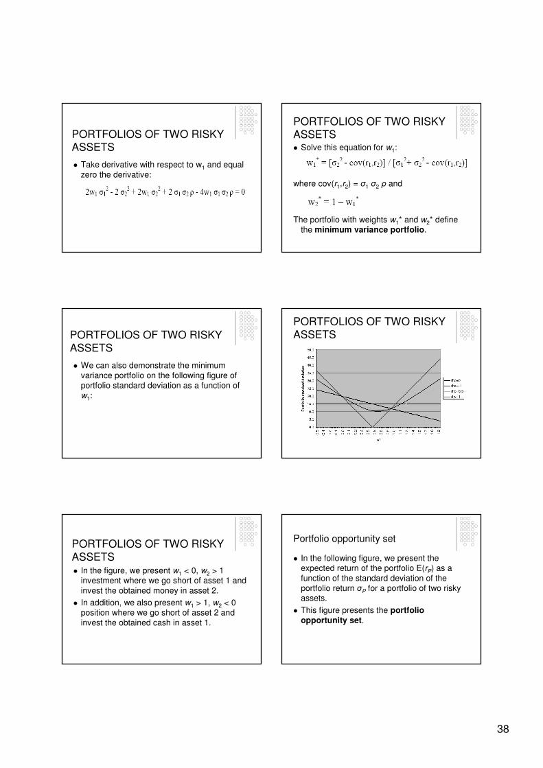
PORTFOLIOS OF TWO RISKY
ASSETS
� We can also demonstrate the minimum
variance portfolio on the following figure of portfolio standard deviation as a function of
w1:
PORTFOLIOS OF TWO RISKY
ASSETS
PORTFOLIOS OF TWO RISKY
ASSETS� In the figure, we present w1 < 0, w2 > 1
investment where we go short of asset 1 and
invest the obtained money in asset 2.
� In addition, we also present w1 > 1, w2 < 0 position where we go short of asset 2 and
invest the obtained cash in asset 1.
Portfolio opportunity set
� In the following figure, we present the expected return of the portfolio E(rP) as a
function of the standard deviation of the portfolio return σP for a portfolio of two risky assets.
� This figure presents the portfolio opportunity set.

39
Portfolio opportunity set Portfolio opportunity set
� The portfolio opportunity set shows the combination of expected return and standard
deviation of all portfolios that can be constructed from the two available risky assets.
Portfolio opportunity set
� The straight line corresponding to the ρ = 1 case shows that there is no benefit from
diversification when perfect correlation of the two risky assets is observed.
Portfolio opportunity set
� The lowest value of the correlation coefficient is ρ = -1. When this case happens than the
investor has the opportunity of creating a perfectly hedged position by choosing the
portfolio weights as follows:
w1 = σ2 / (σ1 + σ2) and
w2 = σ1 / (σ1 + σ2) = 1 – w1
� When these weights are chosen then σP = 0.
EFFICIENT AND MINIMUM VARIANCE FRONTIERS
On the following figure we introduce the
1. Minimum variance frontier and the
2. Efficient frontier
on the portfolio opportunity set.
� Notice that on the minimum variance frontier for each standard deviation there are two alternative expected returns (a high and a low expected return).
� The efficient frontier contains only the higher expected return risky portfolio.
EFFICIENT AND MINIMUM VARIANCE FRONTIERS
40
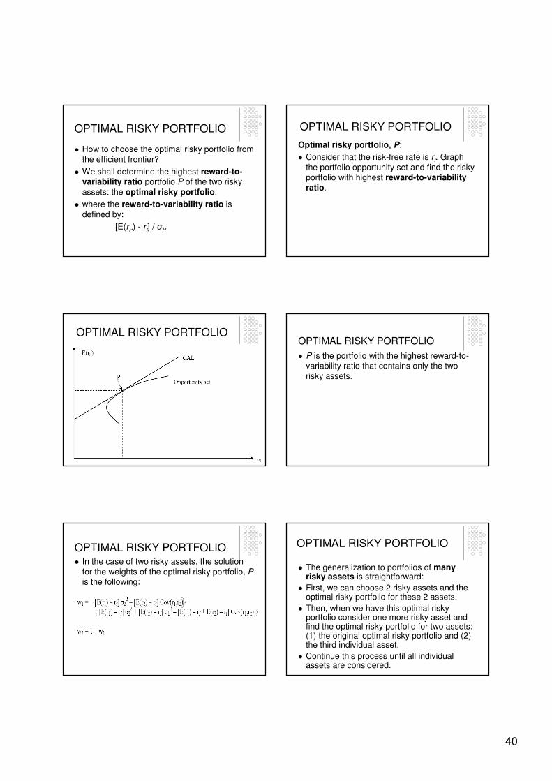
OPTIMAL RISKY PORTFOLIO
� How to choose the optimal risky portfolio from the efficient frontier?
� We shall determine the highest reward-to-variability ratio portfolio P of the two risky
assets: the optimal risky portfolio.
� where the reward-to-variability ratio is defined by:
[E(rP) - rf] / σP
OPTIMAL RISKY PORTFOLIO
Optimal risky portfolio, P:
� Consider that the risk-free rate is rf. Graph
the portfolio opportunity set and find the risky portfolio with highest reward-to-variabilityratio.
OPTIMAL RISKY PORTFOLIOOPTIMAL RISKY PORTFOLIO
� P is the portfolio with the highest reward-to-variability ratio that contains only the two
risky assets.
OPTIMAL RISKY PORTFOLIO� In the case of two risky assets, the solution
for the weights of the optimal risky portfolio, Pis the following:
OPTIMAL RISKY PORTFOLIO
� The generalization to portfolios of many risky assets is straightforward:
� First, we can choose 2 risky assets and the optimal risky portfolio for these 2 assets.
� Then, when we have this optimal risky portfolio consider one more risky asset and find the optimal risky portfolio for two assets: (1) the original optimal risky portfolio and (2) the third individual asset.
� Continue this process until all individual assets are considered.
41
STEP 2:OPTIMAL COMPLETE PORTFOLIO
OPTIMAL COMPLETE PORTFOLIO
� How to combine optimally the optimal risky portfolio with the risk-free asset?
� We shall combine the risk-free asset with portfolio P in order to determine the complete portfolio with highest utility: the optimal complete portfolio.
� The choice of the optimal complete portfolio is called capital allocation decision.
THE RISK FREE ASSET
� Before entering into the details of the capital allocation decision, we review the definition and the properties of the risk-free asset.
� It is a common practice to view Treasury bills (T-bills) as the risk free asset.
� The reason is that only the government has the power to tax and control the money supply and so issue default-free bonds.
THE RISK FREE ASSET
� However, even the default-free guarantee by itself is not sufficient to make the bonds risk-
free in real terms.
� The only risk-free asset in real terms would
be a perfectly price-indexed bond
� Price-indexed means that the bond is indexed against the inflation.
THE RISK FREE ASSET
� Moreover, the price-indexed bond offers a guaranteed real rate to the investor only ifthe maturity of the bond is equal to the investor’s desired holding period.
� Therefore, risk-free asset in real terms does not exist in practice.
� It only exists in nominal terms.
THE RISK FREE ASSET
� In practice, most investors use money market instruments as a risk-free asset.
� These assets are virtually free of any interest rate risk because of their short maturities and
because they are safe in terms of default or credit risk.
42
THE RISK FREE ASSET
Money market funds for most part contain three assets:
� Treasury bills – issued by the government
� Bank certificates of deposit (CD) – issued by banks
� Commercial papers (CP) – issued by well-
know companies
Capital allocation decision
� Capital allocation decision: the choice of the proportion of the risk-free security and the
optimal risky portfolio.
� The investor wants to choose the proportion
of the optimal risky portfolio, y and that of the risk-free asset, 1-y.
Capital allocation decision� Denote f the risk-free asset, P the risky
portfolio and C the complete portfolio of the risky and the risk-free assets.
� Let rf denote the rate of return of the risk-free asset, let E(rP) denote the expected return of the risky portfolio and let E(rC) be the expected return of the complete portfolio.
� Moreover, let σP denote the standard deviation of the risky portfolio and let σC be that of the complete portfolio.
Capital allocation decision
� Then, the expected return and the risk of the complete portfolio, C can be written as
follows:
E(rC) = y E(rP) + (1-y) rf (1)
and
σC = y σP (2)
Capital allocation decision
� Substituting (2) into (1) and rearranging the equation we get the expression of E(rC) as a
function of σC:
E(rC) = rf + σC [E(rP) - rf] / σP (3)
Investment opportunity set or capital allocation line (CAL)
Graph equation (3) in the following figure:
43
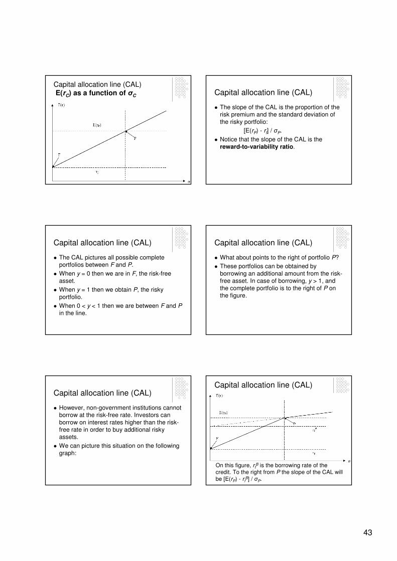
Capital allocation line (CAL)E(rC) as a function of σC Capital allocation line (CAL)
� The slope of the CAL is the proportion of the risk premium and the standard deviation of
the risky portfolio:
[E(rP) - rf] / σP.
� Notice that the slope of the CAL is the
reward-to-variability ratio.
Capital allocation line (CAL)
� The CAL pictures all possible complete portfolios between F and P.
� When y = 0 then we are in F, the risk-free asset.
� When y = 1 then we obtain P, the risky
portfolio.
� When 0 < y < 1 then we are between F and Pin the line.
Capital allocation line (CAL)
� What about points to the right of portfolio P?
� These portfolios can be obtained by
borrowing an additional amount from the risk-free asset. In case of borrowing, y > 1, and
the complete portfolio is to the right of P on the figure.
Capital allocation line (CAL)
� However, non-government institutions cannot borrow at the risk-free rate. Investors can
borrow on interest rates higher than the risk-free rate in order to buy additional risky assets.
� We can picture this situation on the following
graph:
Capital allocation line (CAL)
On this figure, rfB is the borrowing rate of the
credit. To the right from P the slope of the CAL will be [E(rP) - rf
B] / σP.
44
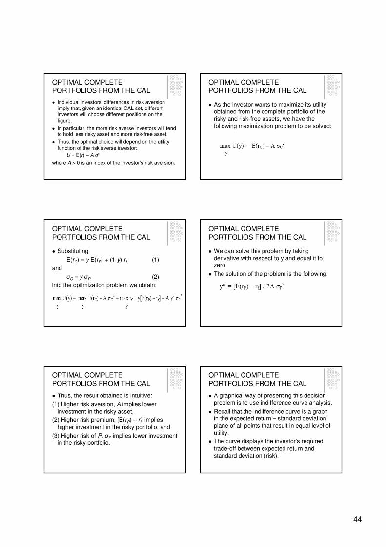
OPTIMAL COMPLETE PORTFOLIOS FROM THE CAL
� Individual investors’ differences in risk aversion imply that, given an identical CAL set, different investors will choose different positions on the
figure.
� In particular, the more risk averse investors will tend
to hold less risky asset and more risk-free asset.
� Thus, the optimal choice will depend on the utility function of the risk averse investor:
U = E(r) – A σ2
where A > 0 is an index of the investor’s risk aversion.
OPTIMAL COMPLETE PORTFOLIOS FROM THE CAL
� As the investor wants to maximize its utility obtained from the complete portfolio of the
risky and risk-free assets, we have the following maximization problem to be solved:
OPTIMAL COMPLETE PORTFOLIOS FROM THE CAL
� Substituting
E(rC) = y E(rP) + (1-y) rf (1)
and
σC = y σP (2)
into the optimization problem we obtain:
OPTIMAL COMPLETE PORTFOLIOS FROM THE CAL
� We can solve this problem by taking derivative with respect to y and equal it to
zero.
� The solution of the problem is the following:
OPTIMAL COMPLETE PORTFOLIOS FROM THE CAL
� Thus, the result obtained is intuitive:
(1) Higher risk aversion, A implies lower investment in the risky asset,
(2) Higher risk premium, [E(rP) – rf] implies higher investment in the risky portfolio, and
(3) Higher risk of P, σP implies lower investment
in the risky portfolio.
OPTIMAL COMPLETE PORTFOLIOS FROM THE CAL
� A graphical way of presenting this decision problem is to use indifference curve analysis.
� Recall that the indifference curve is a graph
in the expected return – standard deviation plane of all points that result in equal level of utility.
� The curve displays the investor’s required
trade-off between expected return and standard deviation (risk).
45
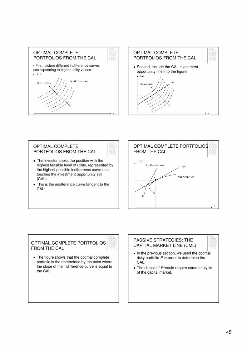
OPTIMAL COMPLETE PORTFOLIOS FROM THE CAL
• First, picture different indifference curves
corresponding to higher utility values:
OPTIMAL COMPLETE PORTFOLIOS FROM THE CAL
� Second, include the CAL investment opportunity line into the figure:
OPTIMAL COMPLETE PORTFOLIOS FROM THE CAL
� The investor seeks the position with the highest feasible level of utility, represented by
the highest possible indifference curve that touches the investment opportunity set (CAL).
� This is the indifference curve tangent to the
CAL:
OPTIMAL COMPLETE PORTFOLIOS
FROM THE CAL
OPTIMAL COMPLETE PORTFOLIOS
FROM THE CAL
� The figure shows that the optimal complete portfolio is the determined by the point where
the slope of the indifference curve is equal to the CAL.
PASSIVE STRATEGIES: THE CAPITAL MARKET LINE (CML)
� In the previous section, we used the optimal risky portfolio P in order to determine the
CAL.
� The choice of P would require some analysis of the capital market.
46
CAPITAL MARKET LINE (CML)
� One possibility would be to avoid of doing any analysis and follow the so-called passive strategy.
� This means that P would represent a broad index of risky assets, for example the S&P500 or IBEX-35 stock index.
� In this case, P is chosen without any capital
market analysis and the resulting CAL is called the capital market line (CML).
CAPITAL MARKET LINE (CML)
� Why would an investor follow the passive strategy of asset allocation?
(1) It is cheap: The alternative active strategy
is not free. For the capital market analysis the investor has fees and other costs.
CAPITAL MARKET LINE (CML)
(2) Free rider benefit: In a competitive capital market, a well-diversified portfolio of common stocks will be a reasonably fair buy, and the passive strategy may not be inferior to that of the average active investor.
� That is by the passive strategy we are free riding on active knowledgeable investors who make stock prices a fair buy.
NOTE: THE SEPARATION PROPERTY
� The determination of the optimal risky portfolio P is independent of the preferences
of the investors.
� Therefore, the portfolio manager will offer the same P to all clients regardless of their degree of risk aversion.
� Thus, the solution of step (1) and (2) can be
separated completely.
� This is called the separation property.
NOTE: THE SEPARATION PROPERTY
� Step 1, the determination of the optimal risky portfolio, P is purely technical.
� Step 2, the determination of the optimal complete portfolio, C depends on the client’s
preferences.
� The separation property makes professional management more efficient and less costly.

47
FACTOR MODELS IN THE CAPITAL MARKETS
MOTIVATION FOR FACTOR MODELS
� The Markowitz portfolio selection model uses the following inputs to form optimal
portfolios:
� (1) expected return of each security
� (2) variance-covariance matrix of security returns.
MOTIVATION FOR FACTOR MODELS
� These inputs the analyist should estimate from empirical data.
� In the followings, we show how many parameters must be estimated in the
Markowitz model.
MOTIVATION FOR FACTOR MODELS
� To find the optimal mean-variance portfolio of n securities, we need to estimate:
� n estimates of expected returns
� n estimates of variances
� (n2 – n)/2 estimates of covariances
� TOTAL = 2n + (n2 – n)/2 estimates of parameters
MOTIVATION FOR FACTOR MODELS
� If n = 1,600 (roughly the number of stocks at New York Stock Exchange, NYSE) then
TOTAL = 1.3 million parameters to be estimated.
� This is impossible from statistical point of view because the number of data
observed is much less than the number of parameters to be estimated.
MOTIVATION FOR FACTOR MODELS
� As the classical Markowitz model is not feasible for large portfolios, alternative
models have appeared in finance, which simplified the model and included much
lower number of parameters than the Markowitz framework.
48
MOTIVATION FOR FACTOR MODELS
� In the followings, the so-called ‘factor models’ are presented.
� In these models, the return of an individual security is driven by one or more common
factors.
� Three alternative factor-models will be presented:
FACTOR MODELS
� We present three alternative ‘factor models’ of
asset returns:
(1) The Capital Asset Pricing Model (CAPM)
(2) Index models
(3) Arbitrage Pricing Theory (APT)
CAPITAL ASSET
PRICING MODEL
(CAPM)
Capital Asset Pricing Model (CAPM)
� The CAPM is a central model of modern financial economics.
� The model gives a precise prediction of the relationship the risk of an asset and its
expected return.
� The CAPM derives that the expected return of a security is driven by a common
‘market’ risk premium.
Capital Asset Pricing Model (CAPM)
� The CAPM is useful because
� (a) It provides a benchmark rate of expected return for evaluating possible
investments of given risk.
� (b) It suggests and alternative measure of risk called “beta”, β.
Capital Asset Pricing Model (CAPM)
� Harry Markowitz laid down the foundations of portfolio theory in 1952.
� Based on his work the CAPM was developed by William Sharpe, John
Lintner and Jan Mossin in three articles over 1964-1966.
� Sharpe received the Nobel Prize in
Economics in 1990.
49
ASSUMPTIONS OF CAPM
� The CAPM is built on a number of simplifying assumptions:
Assumption 1
� There are many investors, each with wealth that is small compared to the total
wealth of all investors.
� Therefore, investors are price takers: security prices are not affected by
investors’ own trades.
� This is the perfect competitionassumption of microeconomics.
Assumption 2
� All investors plan for one identical holding period.
� There is only one period of the CAPM’seconomy.
Assumption 3
� Investments are limited to a universe of publicly traded financial assets such as
stocks, bonds, and to risk-free borrowing or lending arrangements.
Assumption 4
� Investors pay no taxes on returns and no transaction costs on trades in securities.
Assumption 5
� All investors are rational mean-variance optimizers.
� This means that they all use the Markowitz portfolio selection model.
50
Assumption 6
� All investors analyze securities in the same way and share the same economic
view of the world.
� All investors derive the same input list to feed into the Markowitz model.
� This is referred to as homogenous expectations or beliefs.
SUMMARY OF THE CAPM
� In the following slides, some key conclusions of the CAPM are summarized
in several points.
Point 1: All investors hold the market portfolio
� All investors will choose to hold a portfolio of risky assets in portions that duplicate representation of the assets in the market portfolio which includes all traded assets.
� The proportion of each stock in the market portfolio equals the market value of the stock divided by the total market value of all stocks.
� Note: Market value = price per share x number of shares outstanding
Point 1: All investors hold the market portfolio
� If all investors use identical Markowitz
analysis (Assumption 5) applied to the same set of securities (Assumption 3) for
the same time horizon (Assumption 2) and share the same beliefs (Assumption
6), they all must arrive to the same determination of the optimal risky portfolio.
Point 1: All investors hold the market portfolio
� If all investors hold an identical risky portfolio, this portfolio has to be the market
portfolio, M.
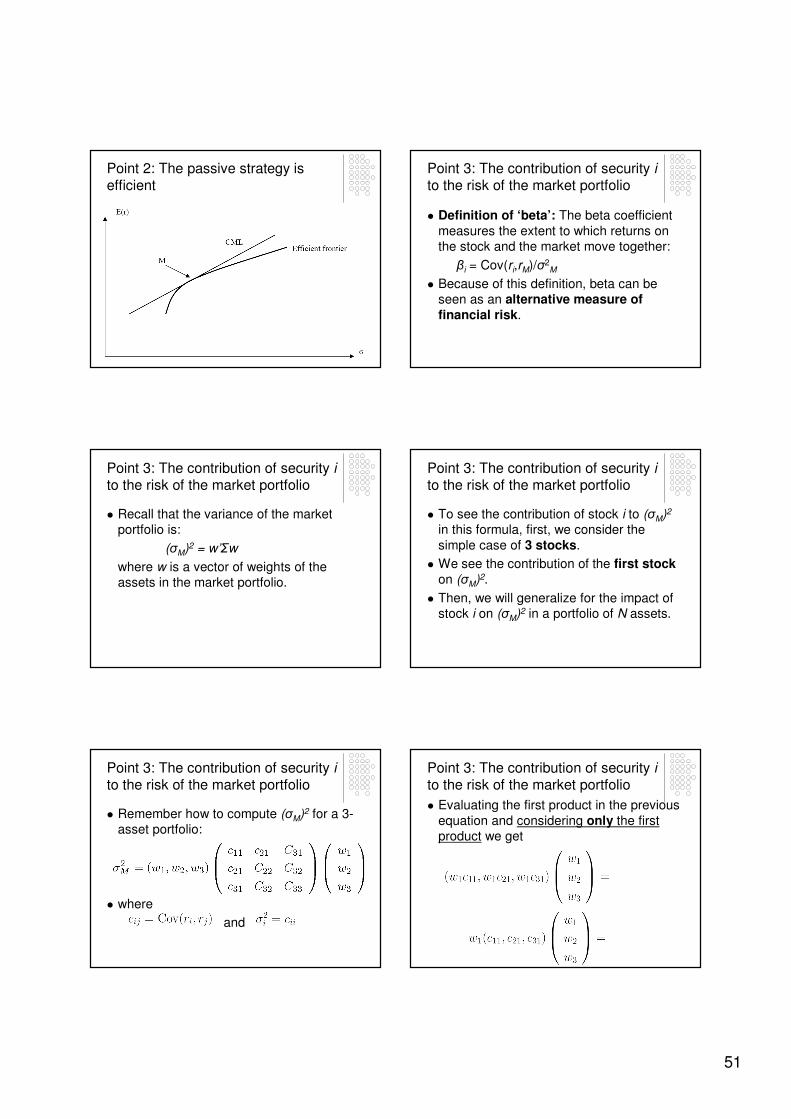
Point 2: The passive strategy is efficient
The market portfolio will be on the:
(a) Efficient frontier and the
(b) Capital allocation line (CAL) derived by each and every investor.
� Therefore, the CAL becomes CML and
� the CML (capital market line) is the tangency portfolio on the efficient frontier.
� See the following figure:
51
Point 2: The passive strategy is efficient
Point 3: The contribution of security ito the risk of the market portfolio
� Definition of ‘beta’: The beta coefficient
measures the extent to which returns on the stock and the market move together:
βi = Cov(ri,rM)/σ2M
� Because of this definition, beta can be seen as an alternative measure of financial risk.
Point 3: The contribution of security ito the risk of the market portfolio
� Recall that the variance of the market portfolio is:
(σM)2 = w’Σw
where w is a vector of weights of the assets in the market portfolio.
Point 3: The contribution of security ito the risk of the market portfolio
� To see the contribution of stock i to (σM)2
in this formula, first, we consider the
simple case of 3 stocks.
� We see the contribution of the first stockon (σM)2.
� Then, we will generalize for the impact of stock i on (σM)2 in a portfolio of N assets.
Point 3: The contribution of security ito the risk of the market portfolio
� Remember how to compute (σM)2 for a 3-asset portfolio:
� where
and
Point 3: The contribution of security ito the risk of the market portfolio
� Evaluating the first product in the previous
equation and considering only the first product we get
52
Point 3: The contribution of security ito the risk of the market portfolio
� Then, evaluating the second product we
get
� This formula tells us the impact of the first
stock on the variance of the 3-asset portfolio.
Point 3: The contribution of security ito the risk of the market portfolio
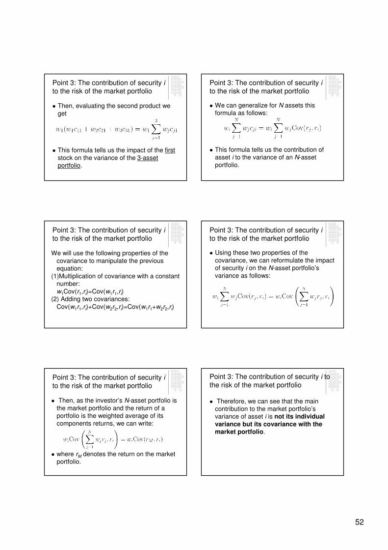
� We can generalize for N assets this formula as follows:
� This formula tells us the contribution of asset i to the variance of an N-asset
portfolio.
Point 3: The contribution of security ito the risk of the market portfolio
We will use the following properties of the
covariance to manipulate the previous equation:
(1)Multiplication of covariance with a constant number:
w1Cov(r1,ri)=Cov(w1r1,ri)(2) Adding two covariances:
Cov(w1r1,ri)+Cov(w2r2,ri)=Cov(w1r1+w2r2,ri)
Point 3: The contribution of security ito the risk of the market portfolio
� Using these two properties of the
covariance, we can reformulate the impact of security i on the N-asset portfolio’s
variance as follows:
Point 3: The contribution of security ito the risk of the market portfolio
� Then, as the investor’s N-asset portfolio is
the market portfolio and the return of a portfolio is the weighted average of its
components returns, we can write:
� where rM denotes the return on the market portfolio.
Point 3: The contribution of security i to
the risk of the market portfolio
� Therefore, we can see that the main contribution to the market portfolio’s variance of asset i is not its individual variance but its covariance with the market portfolio.
53
Point 4: The expected return of security i
� Result: The risk premium on individualassets will be proportional to the risk
premium on the market portfolio, M and the beta coefficient of the security:
E(ri) – rf = βi [ E(rM) – rf ]
� Rearranging this equation, we get the CAPM formula used by practitioners:
E(ri) = rf + βi [ E(rM) – rf ]
Point 4: The expected return of security i
� To determine the appropriate risk premium of security i, we consider two alternative
investments.
� In both cases, initially, the investor holds
100% the market portfolio.
Point 4: The expected return of security i
� Then, the investor modifies its initial
position in two alternative ways.
� We will compare the expected return and the risk of each alternatives and use an
equilibrium argument to derive the risk premium of asset i.
Point 4: The expected return of security i
FIRST INVESTMENT:
(1) The investor holds 100% a market portfolio and wants to increase his position
in the market portfolio by δ percentage.
� The δ percentage of the increase in the market portfolio is borrowed at the risk-
free rate rf.
Point 4: The expected return of security i
The investor’s new portfolio has the
following three elements:
1. the original position in the market
portfolio with return rM
2. a short position of size δ in the risk-free asset with return -δrf
3. a long position of size δ in the market
portfolio with return δrM
Point 4: The expected return of security i
� First, we compute the change in the expected return of the portfolio:
� The new portfolio’s rate of return will be:
rM + δ (rM - rf)
� Taking expectations and comparing with the original expected return E(rM), the
incremental expected rate of return will be
� ∆E(r) = δ [E(rM) - rf] (1)
54
Point 4: The expected return of security i
� Second, we compute the change in the
variance of the portfolio:
� The new portfolio has weight (1 + δ) in the
market portfolio and weight –δ in the risk-free asset.
� Therefore, the new value of portfolio
variance is given by
σ2 = (1 + δ)2 σ2M = (1 + 2δ + δ2) σM
2 = σM
2 + (2δ + δ2) σM2
Point 4: The expected return of security i
� However, if δ is very small then δ2 is negligible compared to 2δ so we can drop
the last term of the previous equation and the new variance can be written as
σ2 = σ2M + 2δ σ2
M
� Therefore, the incremental variance of the
portfolio is given by
∆σ2 = 2δ σ2M (2)
Point 4: The expected return of security i
� The proportion of equations (1) and (2) is called the marginal price of risk.
� In the FIRST INVESTMENT, the marginal price of risk is given by
∆E(r) / ∆σ2 = [E(rM) - rf] / 2 σ2M (3)
Point 4: The expected return
of security i
SECOND INVESTMENT :
(2) The investor initially holds 100% in the
market portfolio and decides to increase the portfolio value by fraction δ investing in
stock i.
� Again the δ fraction is financed by borrowing at the risk-free rate rf.
� The new portfolio has weight 1 in the market portfolio, δ in stock i and -δ in the
risk-free asset.
Point 4: The expected return of security i
� First, the new portfolio’s rate of return will
be:
rM + δ (ri - rf)
� Taking expectations and comparing with
the original expected return E(rM), the incremental expected rate of return will be
∆E(r) = δ [E(ri) - rf] (4)
Point 4: The expected return of security i
� Second, the new portfolio variance is
σ2M + δ2 σ2
i + 2δ Cov(ri,rM)
� Therefore, the increase in the variance is
∆σ2 = δ2 σ2i + 2δ Cov(ri,rM) (5)
55
Point 4: The expected return of security i
� Dropping the negligible δ2 σ2i first term, we
get:
∆σ2 = 2δ Cov(ri,rM) (6)
� Computing the proportion of equations (4)
and (6), we obtain that the marginal price of risk of the SECOND INVESTMENT is
∆E(r) / ∆σ2 = [E(ri) - rf] / 2 Cov(ri,rM) (7)
Point 4: The expected return of security i
� In equilibrium, the marginal price of risk of the two alternatives should equal.
� Therefore, equation (3) should equal equation (7):
[E(rM) - rf] / 2 σ2M =
[E(ri) - rf] / 2 Cov(ri,rM) (8)
Point 4: The expected return of security i
� Rearranging equation (8), we can express the fair risk premium of stock i:
E(ri) - rf = [E(rM) - rf] Cov(ri,rM) / σ2M
(9)
� The term Cov(ri,rM) / σ2M measures the
contribution of the i-th stock to the variance of the market portfolio as a
fraction of the total variance of the market portfolio.
� This term is called “beta” and denoted β.
Point 4: The expected return of security i
� Using this measure, we can restate equation (9) as follows:
E(ri) = rf + βi [E(rM) - rf] (10)
� This expected return – beta relationship is the most familiar expression of the CAPM
to practitioners.
Point 5: Security market line -SML
� We can view the expected return – beta relationship as a reward-risk equation.
� The beta of a security is an appropriate
measure of the risk of the security because beta is proportional to the risk
that the security contributes to the optimal risky portfolio (i.e. the market portfolio).
Point 5: Security market line -SML
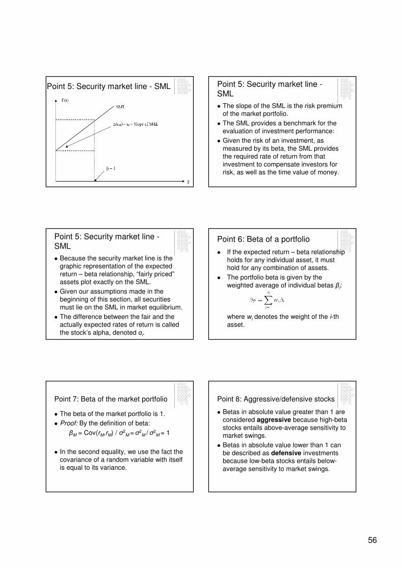
� The expected return – beta relationship of CAPM can be plotted graphically as the
security market line (SML):
E(ri) = rf + βi [E(rM) - rf]
56
Point 5: Security market line - SML Point 5: Security market line -SML
� The slope of the SML is the risk premium of the market portfolio.
� The SML provides a benchmark for the evaluation of investment performance:
� Given the risk of an investment, as
measured by its beta, the SML provides the required rate of return from that
investment to compensate investors for risk, as well as the time value of money.
Point 5: Security market line -SML
� Because the security market line is the graphic representation of the expected
return – beta relationship, “fairly priced”assets plot exactly on the SML.
� Given our assumptions made in the beginning of this section, all securities
must lie on the SML in market equilibrium.
� The difference between the fair and the actually expected rates of return is called
the stock’s alpha, denoted αi.
Point 6: Beta of a portfolio
� If the expected return – beta relationship
holds for any individual asset, it must hold for any combination of assets.
� The portfolio beta is given by the
weighted average of individual betas βi:
where wi denotes the weight of the i-th
asset.
Point 7: Beta of the market portfolio
� The beta of the market portfolio is 1.
� Proof: By the definition of beta:
βM = Cov(rM,rM) / σ2M = σ2
M / σ2M = 1
� In the second equality, we use the fact the
covariance of a random variable with itself is equal to its variance.
Point 8: Aggressive/defensive stocks
� Betas in absolute value greater than 1 are considered aggressive because high-beta
stocks entails above-average sensitivity to market swings.
� Betas in absolute value lower than 1 can
be described as defensive investments because low-beta stocks entails below-
average sensitivity to market swings.
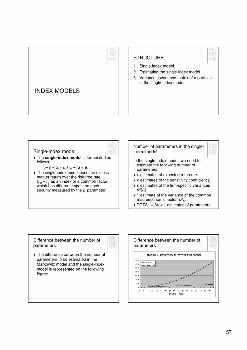
57
INDEX MODELS
STRUCTURE
1. Single-index model
2. Estimating the single-index model
3. Variance covariance matrix of a portfolio in the single-index model
Single-index model� The single-index model is formulated as
follows:
ri – rf = αi + βi (rM – rf) + ei
� The single-index model uses the excess market return over the risk-free rate, (rM – rf) as an index or a common factor, which has different impact on each security measured by the βi parameter.
Number of parameters in the single-index model
In the single-index model, we need to estimate the following number of parameters:
� n estimates of expected returns αi
� n estimates of the sensitivity coefficient βi
� n estimates of the firm-specific variances σ2(ei)
� 1 estimate of the variance of the common macroeconomic factor, σ2
M.
� TOTAL = 3n + 1 estimates of parameters.
Difference between the number of parameters
� The difference between the number of parameters to be estimated in the
Markowitz model and the single-index model is represented on the following
figure:
Difference between the number of parameters
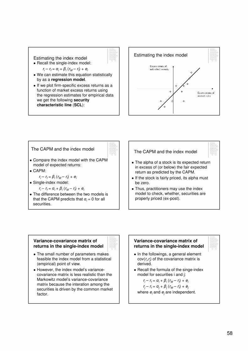
58
Estimating the index model� Recall the single-index model:
ri – rf = αi + βi (rM – rf) + ei
� We can estimate this equation statistically by as a regression model.
� If we plot firm-specific excess returns as a function of market excess returns using
the regression estimates for empirical data we get the following security characteristic line (SCL):
Estimating the index model
The CAPM and the index model
� Compare the index model with the CAPM model of expected returns:
� CAPM:
ri – rf = βi (rM – rf) + ei
� Single-index model:
ri – rf = αi + βi (rM – rf) + ei
� The difference between the two models is that the CAPM predicts that αi = 0 for all
securities.
The CAPM and the index model
� The alpha of a stock is its expected return in excess of (or below) the fair expected
return as predicted by the CAPM.
� If the stock is fairly priced, its alpha must
be zero.
� Thus, practitioners may use the index model to check, whether, securities are
properly priced (ex-post).
Variance-covariance matrix of returns in the single-index model
� The small number of parameters makes feasible the index model from a statistical
(empirical) point of view.
� However, the index model’s variance-covariance matrix is less realistic than the
Markowitz model’s variance-covariance matrix because the interation among the
securities is driven by the common market factor.
Variance-covariance matrix of returns in the single-index model
� In the followings, a general element cov(ri,rj) of the covariance matrix is
derived.
� Recall the formula of the singe-index model for securities i and j:
ri – rf = αi + βi (rM – rf) + ei
rj – rf = αj + βj (rM – rf) + ej
where ei and ej are independent.

59
Variance-covariance matrix of returns in the single-index model
� Substituting these equations into the covariance of returns i and j we get:
� cov(ri,rj) =
� cov(αi+βi(rM–rf)+ei,αj+βj(rM–rf)+ej)
Variance-covariance matrix of returns in the single-index model
� Using the properties of covariance and the independence of ei and ej we get:
cov(αi+βi(rM–rf)+ei,αj+βj(rM–rf) + ej) =
cov(βi(rM–rf)+ei,βj(rM–rf) + ej) =
cov(βi(rM–rf),βj(rM–rf)) =
βiβjcov((rM–rf),(rM–rf)) =
βiβjcov(rM,rM) =
βiβjVar(rM) = βiβj(σM)2
Variance-covariance matrix of returns in the single-index model
� As a consequence, the covariance matrix
of a portfolio can be computed by using the beta parameters estimated for all
assets in the portfolio and the estimate of the market variance:
cov(ri,rj) = βiβj(σM)2
� We can use this variance-covariance matrix as an input to the Markowitz model
to find the optimal portfolio.
ARBITRAGE PRICING
THEORY (APT)
STRUCTURE
1. Motivation
2. Arbitrage pricing theory (APT)
3. Comparison of APT and CAPM
4. Variance-covariance matrix of the two-
factor APT model
MOTIVATION� Theoretically and empirically, one of the
most troubling problems of CAPM for academics and managers has been that
the CAPM’s single source of risk is the market.
� They believe that the market is not the only factor that is important in determining
the return an asset is expected to earn.
� The CAPM is sometimes called a single-factor model.
60
MOTIVATION
� As a consequence, both academics and practitioners have analyzed the influence of adding additional factors into the CAPM equation.
� For example, additional factors considered have been:
1. Price/earnings ratios
2. Stock-issue size (volume)
3. Liquidity
4. Taxes
MOTIVATION
� Practitioners believed that these factors were important, and academic studies
appeared to show they were important.
� These academic studies have used so-called multi-factor models.
� The most famous multi-factor model, the
arbitrage pricing theory (APT), was developed by Steven Ross in 1976.
Arbitrage Pricing Theory (APT)
� The risk premium of a risky asset in APT
can be written as
ri – rf = ai + βi1(F1 – rf) +…+ βin(Fn – rf) + ei
where Fj, j = 1,…,n denotes the factor, that
is, the systematic component of the return, and ei corresponds to the firm-specific
component of the return.
� The ei is assumed to be independent of the factors.
Factors of APT
� The APT does not say what the factors are.
� They could be an oil price factor, an
interest rate factor, etc.
� The return on the market portfolio might
serve as one factor – as in the CAPM –but it might not as well.
Conclusions of APT
� A portfolio that is constructed to have zero sensitivity to each factor is
essentially risk-free and therefore must be priced to offer the risk-free rate of
interest.
� A portfolio that is constructed to have exposure to factor, F1, will offer a risk
premium, which depends on the portfolio’s sensitivity to that factor.
Conclusions of APT
� Example: Imagine that one could construct two portfolios, A and B, that are affected
only by F1.
� If portfolio A is twice as sensitive to factor
F1 as portfolio B, portfolio A must offer twice the risk premium.
� Therefore, a portfolio of 50% U.S. Treasury
bills and 50% portfolio A has exactly the same sensitivity to F1 as portfolio of 100%
portfolio B.
61
Comparison of APT and CAPM
� APT obtains an expected return-beta relationship identical to that of the CAPM,
without the restrictive assumptions of the CAPM.
� This suggests that despite its restrictive
assumptions the main conclusions of the CAPM is likely to be at least approximately
valid.
Comparison of APT and CAPM
� We note that in contrast to the CAPM the APT does not require that the benchmark
portfolio be the true market portfolio.
� Accordingly, the APT has more flexibility than does the CAPM.
Variance-covariance matrix of a portfolio in the two-factor APT model
� We show how to compute a general
element cov(ri,rj) of the covariance matrix of a portfolio in the two-factor APT model.
� Recall this model for securities i and j:
ri – rf = ai + βi1(F1 – rf) + βi2(F2 – rf) + ei
rj – rf = aj + βj1(F1 – rf) + βj2(F2 – rf) + ei
where ei and ej are independent.
Variance-covariance matrix of a portfolio in the two-factor APT model
� Substituting these equations into the covariance of returns i and j we get:
� cov(ri,rj) =
� cov(αi+β1i(F1–rf) +β2i(F2–rf)+ei,
αj+β1j(F1–rf) +β2j(F2–rf)+ej) =
� cov(β1i(F1–rf) +β2i(F2–rf),
β1j(F1–rf) +β2j(F2–rf)) =
Variance-covariance matrix of a portfolio in the two-factor APT model
� cov(β1i(F1–rf) +β2i(F2–rf),
β1j(F1–rf) +β2j(F2–rf)) =
� cov(β1iF1+β2iF2,β1jF1 +β2jF2) =
� cov(β1iF1,β1jF1) + cov(β1iF1,β2jF2) +
cov(β2iF2,β1jF1) + cov(β2iF2,β2jF2) =
� β1iβ1jVar(F1) + β1iβ2jcov(F1,F2) +
β1jβ2icov(F1,F2) + β2iβ2jVar(F2)
Variance-covariance matrix of a portfolio in the two-factor APT model
� As a consequence, the covariance matrix
of a portfolio can be computed by using the beta parameters estimated for all
assets in the portfolio and the estimate of the variances and covariances of the
factors:

62
Variance-covariance matrix of a portfolio in the two-factor APT model
� cov(ri,rj) =
β1iβ1jVar(F1) +
β2iβ2jVar(F2) +
[β1iβ2j+β1jβ2i] cov(F1,F2)
� We can use the variance-covariance
matrix as an input to the Markowitz model to find the optimal portfolio.
63
FINANCIAL MARKETS
FINANCIAL MARKETS
1. PUBLIC FINANCIAL MARKET
where governments borrow money.
For example:
� Treasury bills (T-bill) – short term security,
� Treasury bonds – long term security
2. CORPORATE FINANCIAL MARKET
where enterprises borrow money.
For example:
� Stocks
� Corporate bonds
FINANCIAL MARKETS
1. PRIMARY MARKETS
2. SECONDARY MARKETS
FINANCIAL MARKETS
1. PRIMARY MARKETS
� The primary market is that part of the
capital markets that deals with the issuance of new securities.
� The process of selling new issues to
investors is called underwriting.
� In the case of a new stock issue, this sale is an initial public offering (IPO).
FINANCIAL MARKETS
2. SECONDARY MARKETS
� The secondary market, also known as
the aftermarket, is the financial market where previously issued securities and
financial instruments such as stock, bonds, options, and futures are bought and sold.
FINANCIAL EXCHANGES
Secondary markets can be:
� ORGANIZED MARKETS or
� OVER-THE-COUNTER (OTC) MARKETS

64
FINANCIAL EXCHANGES
1. ORGANIZED MARKETS:
For example
� New York Stock Exchange (NYSE)
� Chicago Board of Trade (CBOT)
� Bolsa de Madrid (= Madrid Stock Exchange)
These are physical markets.
FINANCIAL EXCHANGES
2. OVER-THE-COUNTER (OTC) MARKETS:
For example
� National Association of Securities Dealers (NASD) Automated Quotes(NASDAQ) organized by NASD.
These are electronic markets.

65
FIXED-INCOME SECURITIES
Bond characteristics
� A bond is a security that is issued in connection with a borrowing arrangement.
� The borrower issues (i.e. sells) a bond to the
lender for some amount of cash.
� The arrangement obliges the issuer to make
specified payments to the bondholder on specified dates.
Bond characteristics
� A typical bond obliges the issuer to make semiannual payments of interest to the
bondholder for the life of the bond.
� These are called coupon payments.
� Most bonds have coupons that investors
would clip off and present to claim the interest payment.
Bond characteristics
� When the bond matures, the issuer repays the debt by paying the bondholder the bond’s
par value (or face value).
� The coupon rate of the bond serves to
determine the interest payment:
� The annual payment is the coupon rate times the bond’s par value.
Bond characteristics -typical contract
� The typical bond contract informs about:
1.Coupon rate
2.Par value
3.Maturity date
Bond characteristics –general contract
� A more general bond contract may pay the coupon and par value cash flows at any time before maturity.
� In these bond contracts, the next points are specified:
1. Coupon rate
2. Coupon payment times
3. Par value
4. Par value payment times and values
5. Maturity date
66
Example
� A bond with par value EUR1000 and coupon
rate of 8%.
� The bondholder is then entitled to a payment of 8% of EUR1000, or EUR80 per year, for
the stated life of the bond, 30 years.
� The EUR80 payment typically comes in two
semiannual installments of EUR40 each.
� At the end of the 30-year life of the bond, the issuer also pays the EUR1000 value to the
bondholder.
Zero-coupon bonds
� These are bonds with no coupon payments.
� Investors receive par value at the maturity date
but receive no interest payments until then.
� The bond has a coupon rate of zero percent.
� These bonds are issued at prices considerably below par value, and the investor’s return
comes solely from the difference between issue price and the payment of par value at maturity.
Treasury bonds, notes and bills
� The U.S. government finances its public budget by issuing public fixed-income
securities.
� The maturity of the treasury bond is from 10 to 30 years.
� The maturity of the treasury note is from 1 to 10 years.
� The maturity of the treasury bill (T-bill) is up
to 1 year.
Corporate bonds
Like the governments, corporations borrow money by issuing bonds.
� Although some corporate bonds are traded at
organized markets, most bonds are traded over-the-counter in a computer network of bond dealers.
� As a general rule, safer bonds with higher
ratings promise lower yields to maturity than more risky bonds.
Corporate bonds
� The are several types of corporate bonds related to the specific characteristics of the
bond contract:
1. Call provisions on corporate bonds
2. Puttable bonds
3. Convertible bonds
4. Floating-rate bonds
1. Call provisions on corporate bonds
� Some corporate bonds are issued with call provisions allowing the issuer to repurchase
the bond at a specified call price before the maturity date.
� For example, if a company issues a bond with a high coupon rate when market interest
rates are high, and interest rates later fall, the firm might like to retire the high-coupon debt
and issue new bonds at a lower coupon rate. This is called refunding.

67
1. Call provisions on corporate bonds
� Callable bonds are typically come with a period of call protection, an initial time
during which the bonds are not callable.
� Such bonds are referred to as deferred callable bonds.
2. Puttable bonds
� While the callable bond gives the issuer the option to retire the bond at the call
date, the put bond gives this option to the bondholder.
3. Convertible bonds
� Convertible bonds give bondholders an option to exchange each bond for a
specified number of shares of common stock of the firm.
� The conversion ratio is the number of shares for which each bond may be
exchanged.
3. Convertible bonds
� The market conversion value is the current value of the shares for which the
bonds may be exchanged.
� The conversion premium is the excess
of the bond value over its conversion value.
� Example: If the bond were selling
currently for EUR950 and its conversion value is EUR800, its premium would be
EUR150.
4. Floating-rate bonds
� These bonds make interest payments that are tied to some measure of current
market rates.
� For example, the rate can be adjusted annually to the current T-bill rate plus 2%.
Other specific bonds
� Other bonds (or bond like assets) traded on the market:
1. Preferred stock
2. International bond
3. Bond innovations

68
1. Preferred stock
� Although the preferred stock strictly
speaking is considered to be equity, it can be also considered as a bond.
� The reason is that a preferred stock promises to pay a specified stream of
dividends.
� Preferred stocks commonly pay a fixed dividend.
� Therefore, it is in effect a perpetuity.
1. Preferred stock
� In the last two decades, floating-rate preferred stocks have become popular.
� Floating-rate preferred stock is much like a floating-rate bond:
� The dividend rate is linked to a measure of
current market interest rates and is adjusted at regular intervals.
2. International bonds
� International bonds are commonly divided into two categories:
� 2a. Foreign bonds
� 2b. Eurobonds
2a. International bondsForeign bonds
� Foreign bonds are issued by a borrower from a country other than the one in which
the bond is sold.
� The bond is denominated in the currency
of the country in which it is marketed.
� For example, a German firm sells a dollar-denominated bond in the U.S., the bond is
considered as a foreign bond.
2a. International bondsForeign bonds
� Foreign bonds are given colorful names based on the countries in which they are
marketed:
1. Foreign bonds sold in the U.S. are called Yankee bonds.
2. Foreign bonds sold in Japan are called Samurai bonds.
3. Foreign bonds sold in U.K. are called
bulldog bonds.
2b. International bonds
Eurobonds
� Eurobonds are bonds issued in the currency of one country but sold in other national
markets.
1. The Eurodollar market refers to dollar-denominated Eurobonds sold outside the U.S..
2. The Euroyen bonds are yen-denominated Eurobonds sold outside Japan.
3. The Eurosterling bonds are pound-
denominated Eurobonds sold outside the U.K..
69
Innovations in the bond market
� Issuers constantly develop innovative bonds with unusual features. Some of
these bonds are:
1. Inverse floaters
2. Asset-backed bonds
3. Catastrophe bonds
4. Indexed bonds
1. Inverse floaters
� These are similar to the floating-rate bonds except that the coupon rate on these bonds falls when the general level of interest rates rises.
� Investors suffer doubly when rates rise:
1. The present value of the future bond payments decreases.
2. The level of the future bond payments decreases.
� Investors benefit doubly when rates fall.
2. Asset-backed bonds
� In asset-backed securities, the income from a specific group of assets is used to
service the debt.
� For example, David Bowie bonds have been issued with payments that will be tied
to the royalties on some of his albums.
2. Mortgage-backed bonds
� Another example of asset-backed bondsis mortgage-backed security, which is
either an ownership claim in a pool of mortgages or an obligation that is secured
by such a pool.
� These claims represent securitization of
mortgage loans.
� Mortgage lenders originate loans and then sell packages of these loans in the
secondary market.
2. Mortgage-backed bonds
� The mortgage originator continues to service the loan, collecting principal and
interest payments, and passes these payments to the purchaser of the
mortgage.
� For this reason, mortgage-backed
securities are called pass-throughs.
3. Catastrophe bonds
� Catastrophe bonds are a way to transfer catastrophe risk from a firm to the market.
� For example, Tokyo Disneyland issued a bond with a final payment that depended
on whether there has been an earthquake near the park.
70
4. Indexed bonds
� Indexed bonds make payments that are tied to a general price index or the price of a particular commodity.
� For example, Mexico issued 20-year bonds with payments that depend on the price of oil.
� The U.S. Treasury issued inflation protected bonds in 1997. (Treasury Inflation Protected Securities, TIPS)
� For TIPS, the coupon and final payment is related to the consumer price index.
BOND PRICING
Bond pricing
� Because a bond’s coupon and principal repayments all occur in the future, the price
an investor would be willing to pay for a claim to those payments depends on the value of
dollars to be received in the future compared to dollars in hand today.
� This present value calculation depends on the market interest rates.
Bond pricing
� First, we simplify the present value
calculation by assuming that there is oneinterest rate that is appropriate for
discounting cash flows of any maturity.
� Later, we will relax this assumption and we will use different interest rates for cash flows accruing in different periods.
Bond pricing
� To value a security, we discount its expected cash flows by the appropriate discount rate.
� The cash flows from a bond consist of coupon
payments until the maturity date plus the final payment of par value.
� Therefore,
Bond value = Present value of coupons +
Present value of par value
Bond pricing
� Let r denote the interest rate (discount rate) and T the maturity date of the bond.
� Suppose that the bond has annualcoupon payments.
� Then, the value of the bond is given by:
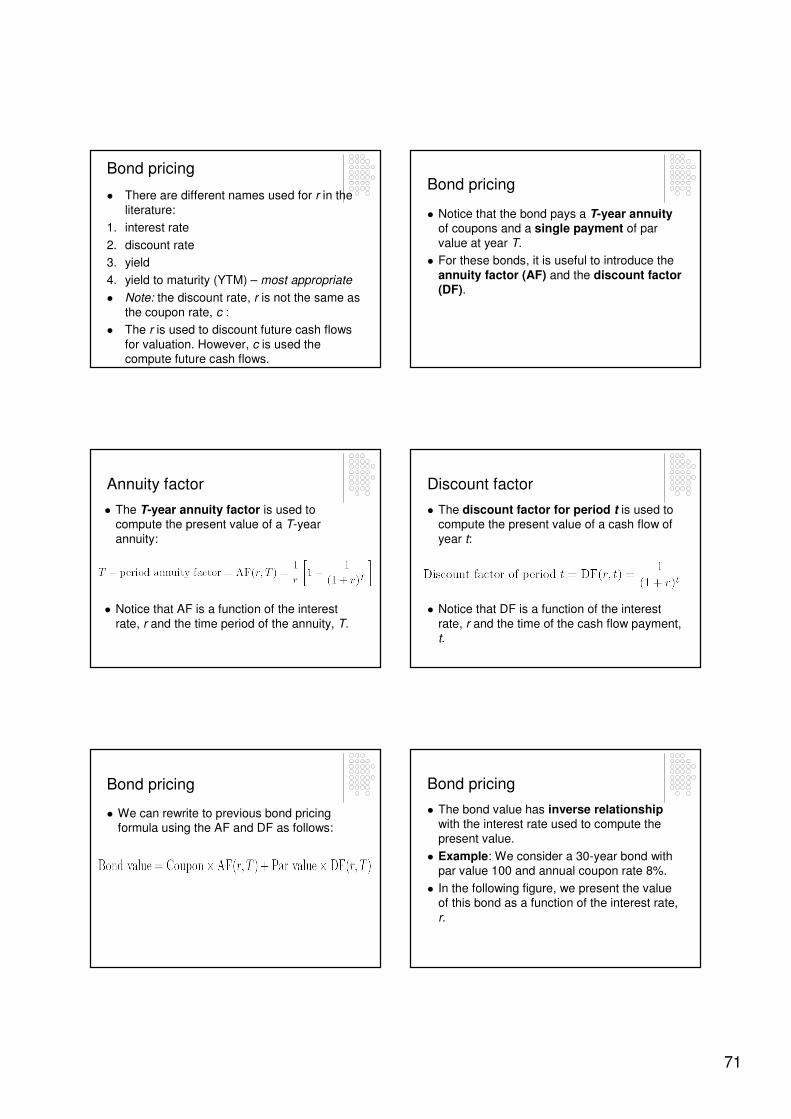
71
Bond pricing
� There are different names used for r in the
literature:
1. interest rate
2. discount rate
3. yield
4. yield to maturity (YTM) – most appropriate
� Note: the discount rate, r is not the same as
the coupon rate, c :
� The r is used to discount future cash flows
for valuation. However, c is used the compute future cash flows.
Bond pricing
� Notice that the bond pays a T-year annuityof coupons and a single payment of par
value at year T.
� For these bonds, it is useful to introduce the
annuity factor (AF) and the discount factor (DF).
Annuity factor
� The T-year annuity factor is used to compute the present value of a T-year
annuity:
� Notice that AF is a function of the interest
rate, r and the time period of the annuity, T.
Discount factor
� The discount factor for period t is used to compute the present value of a cash flow of
year t:
� Notice that DF is a function of the interest
rate, r and the time of the cash flow payment, t.
Bond pricing
� We can rewrite to previous bond pricing formula using the AF and DF as follows:
Bond pricing
� The bond value has inverse relationshipwith the interest rate used to compute the
present value.
� Example: We consider a 30-year bond with par value 100 and annual coupon rate 8%.
� In the following figure, we present the value of this bond as a function of the interest rate,
r.
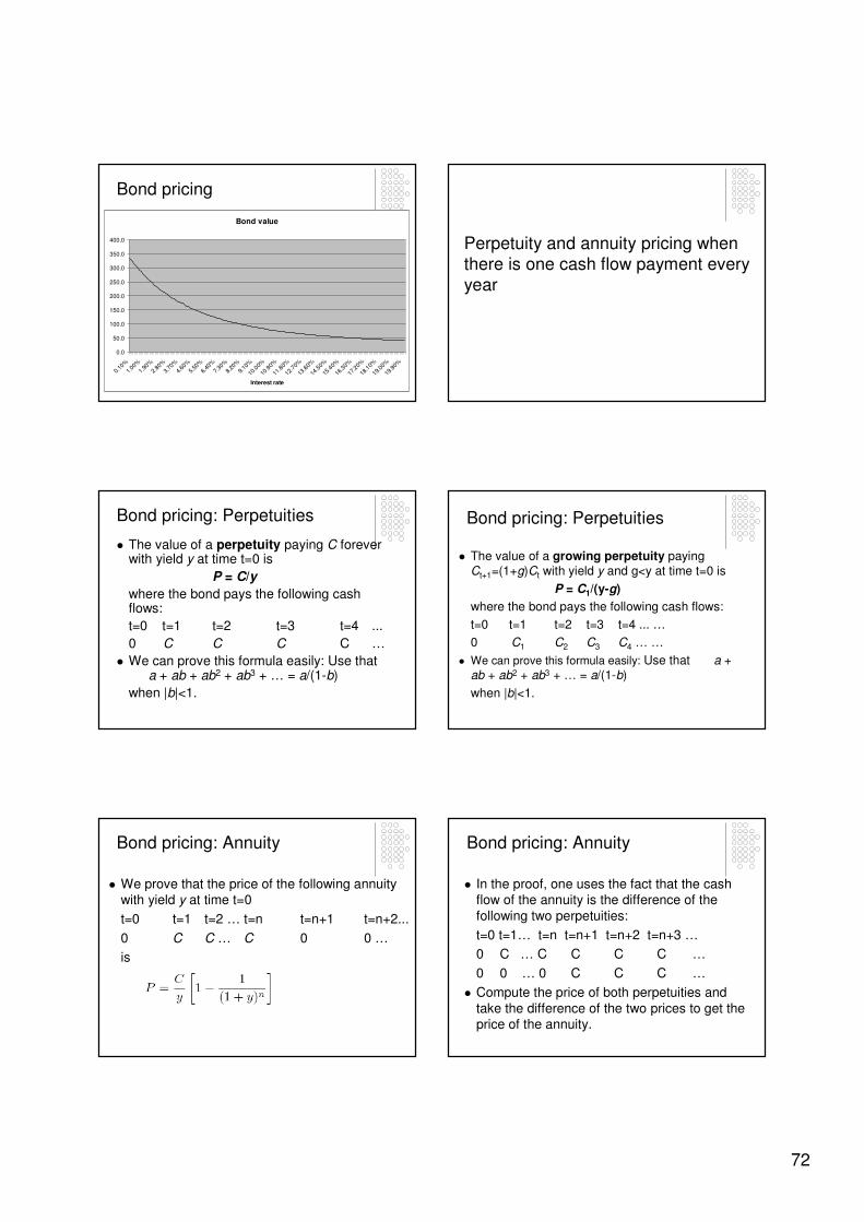
72
Bond pricing
Bond value
0.0
50.0
100.0
150.0
200.0
250.0
300.0
350.0
400.0
0.10
%
1.00
%
1.90
%
2.80
%
3.70
%
4.60
%
5.50
%
6.40
%
7.30
%
8.20
%
9.10
%
10.0
0%
10.9
0%
11.8
0%
12.7
0%
13.6
0%
14.5
0%
15.4
0%
16.3
0%
17.2
0%
18.1
0%
19.0
0%
19.9
0%
Interest rate
Perpetuity and annuity pricing when
there is one cash flow payment every
year
Bond pricing: Perpetuities
� The value of a perpetuity paying C forever with yield y at time t=0 is
P = C/y
where the bond pays the following cash flows:
t=0 t=1 t=2 t=3 t=4 ...
0 C C C C …
� We can prove this formula easily: Use that a + ab + ab2 + ab3 + … = a/(1-b)
when |b|<1.
Bond pricing: Perpetuities
� The value of a growing perpetuity paying Ct+1=(1+g)Ct with yield y and g<y at time t=0 is
P = C1/(y-g)
where the bond pays the following cash flows:
t=0 t=1 t=2 t=3 t=4 ... …
0 C1 C2 C3 C4 … …
� We can prove this formula easily: Use that a + ab + ab2 + ab3 + … = a/(1-b)
when |b|<1.
Bond pricing: Annuity
� We prove that the price of the following annuity with yield y at time t=0
t=0 t=1 t=2 … t=n t=n+1 t=n+2...
0 C C … C 0 0 …
is
Bond pricing: Annuity
� In the proof, one uses the fact that the cash flow of the annuity is the difference of the
following two perpetuities:
t=0 t=1… t=n t=n+1 t=n+2 t=n+3 …
0 C … C C C C …
0 0 … 0 C C C …
� Compute the price of both perpetuities and
take the difference of the two prices to get the price of the annuity.

73
Perpetuity and annuity pricing when
there are n cash flow payments every year

74

75
Bond pricing between coupon dates
Quoted bond prices
� In the financial newspapers, there are two prices presented for each bond:
� The bid price at which one can sell the bond
to a dealer.
� The asked price is the price at which one
can buy the bond from a dealer.
� The asked price is higher than the bid price.
Accrued interest and quoted bond prices
� The bond prices presented in the newspaper are not actually the prices that investors pay
for the bond.
� The prices which appear in financial press are called flat prices.
� This is because the quoted price does not include the interest that accrues between
coupon payment dates.
Accrued interest and quoted bond prices
� The actual invoice price that the buyer pays for the bond includes accrued interest:
Invoice price = Flat price +
Accrued interest
Accrued interest and quoted bond prices
� If a bond is purchased between coupon payments, the buyer must pay the seller for
accrued interest, the prorated share of the upcoming semiannual coupon.
76
Accrued interest and quoted bond prices
� Example: If 30 days have passed since the last coupon payment, and there are 182 days
in the semiannual coupon period, the seller is entitled to a payment of accrued interest of 30/182 of the semiannual coupon.
Accrued interest and quoted bond prices
� In general, the formula for the amount of accrued interest between two dates of the
semiannual payment is
Accrued interest =
(Annual coupon payment /2) x
(Days since last coupon payment /
Days separating coupon payments)
Bond yields
Yield to maturity
� In practice, an investor considering the purchase of a bond is not quoted a promised rate of return.
� Instead, the investor must use the bond price, maturity date, and coupon payments to infer the return offered by the bond over its life.
� The yield to maturity (YTM) is defined as the interest rate that makes the present value of a bond’s payments equal to its price.
Yield to maturity
� The YTM can be interpreted as the annual rate of return on the bond investment given that the investor holds the bond until its maturity.
� Important: YTM can be interpreted as annual return only if the bond is held until maturity.
� It is useful to know the YTM because it can be used to compare the returns obtained on alternative bond investments.
Yield to maturity
� For example, consider the typical bond for
which we observe the bond value (price on the market) and we also know the coupon and par value cash flows.
� The calculate the YTM, we solve the bond pricing equation for the discount rate, r given the bond’s price (bond value):
77
Yield to maturity
� This is a highly non-linear equation in r, therefore we have to use numerical
methods to find the value of r. We can do it in Excel.
� See PRACTICE 2 for an example how to
find YTM for any bond and how it can be used to compare the returns of alternative
bond investments.
Premium and discount bonds
Premium and discount bonds
� In this section, we only consider typical bonds which pay 100% of the face value at maturity. (For example, government
bonds.)
� Define the concepts of premium bond and
discount bond as follows:
� Premium bond: bond with market price above the par value
� Discount bond: bond with market price
below the par value
Current yield -- definition
� We have already seen the YTM and the
coupon rate.
� We also define the current yield of the bond:
� current yield = the bond’s annual coupon
payment divided by the bond price
� On the following slides, we show that there
is an ordering among YTM, current yield and coupon rate.
Premium and discount bonds
� For premium bond, the coupon rate is greater than current yield, which is greater
than yield to maturity:
YTM < Current yield < Coupon rate
� For discount bond, the coupon rate is lower
than current yield, which is lower than yield to maturity:
Coupon rate < Current yield < YTM
TERM STRUCTURE OF
INTEREST RATES

78
TERM STRUCTURE OF INTEREST RATES
� The term structure of interest rates is represented by the yield curve.
� The yield curve is a plot of yield to maturity (YTM) of several bonds as a function of time to maturity.
� In other words, we compute the YTM of
different maturity bonds, then, make a plot of the YTMs as a function of the maturities of
the bonds.
TERM STRUCTURE OF INTEREST RATES
� However, notice that this definition is not precise because two bonds with the same
maturity date may have different YTM values.
� Then, which bond’s YTM to plot on the yield curve?
� The solution is to choose a specific bond:
the zero coupon bond and plot the YTM of zero coupon bonds of the yield curve
plot.
TERM STRUCTURE OF INTEREST RATES
� More precise definition of yield curve:
� The yield curve is a plot of yield to maturity (YTM) of several zero couponbonds as a function of time to maturity.
MOTIVATION FOR YIELD CURVE
� Why is it interesting for practitioners to know the term structure of interest rates?
� Because one can use the yield curve in order to price any fixed income instrument
not traded yet or the check if the market values correctly a given fixed income
instrument.
� For example, a firm wants to issue a new bond and want to set the issue price of this
bond.
TERM STRUCTURE OF
INTEREST RATES - Example
� Suppose that zero-coupon bonds with 1-
year maturity sell at YTM y1=5%, 2-year zeros sell at YTM y2=6% and 3-year zeros
sell at YTM y3=7%.
� Which of these rates should we use to
discount bond cash flows to compute the price of a fourth bond having CF during
the first three years?
TERM STRUCTURE OF INTEREST
RATES - Example
� ALL OF THEM.
� The trick is to:
� (1) consider each cash flow payment of
the fourth bond as a zero-coupon bond,
� (2) price each zero-coupon bond and
� (3) sum the prices of all zero-coupon bonds.
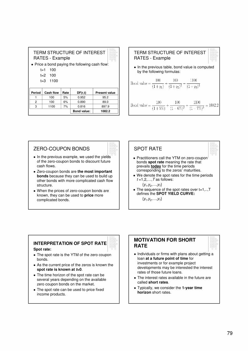
79
TERM STRUCTURE OF INTEREST
RATES - Example
� Price a bond paying the following cash flow:
t=1 100
t=2 100
t=3 1100
1082.2Bond value:
897.90.8167%11003
89.00.8906%1002
95.20.9525%1001
Present valueDF(r,t)RateCash flowPeriod
TERM STRUCTURE OF INTEREST
RATES - Example
� In the previous table, bond value is computed by the following formulas:
ZERO-COUPON BONDS
� In the previous example, we used the yields of the zero-coupon bonds to discount future
cash flows.
� Zero-coupon bonds are the most important bonds because they can be used to build up
other bonds with more complicated cash flow structure.
� When the prices of zero-coupon bonds are known, they can be used to price more
complicated bonds.
SPOT RATE
� Practitioners call the YTM on zero-coupon bonds spot rate meaning the rate that prevails today for the time periods corresponding to the zeros’ maturities.
� We denote the spot rates for the time periods t =1,2,…,T as follows:
{y1,y2,…,yT}
� The sequence of the spot rates over t=1,..,T defines the SPOT YIELD CURVE:
{y1,y2,…,yT}
INTERPRETATION OF SPOT RATE
Spot rate:
� The spot rate is the YTM of the zero coupon
bonds.
� As the current price of the zeros is known the spot rate is known at t=0.
� The time horizon of the spot rate can be several years depending on the available
zero coupon bonds on the market.
� The spot rate can be used to price fixed income products.
MOTIVATION FOR SHORT RATE
� Individuals or firms with plans about getting a loan at a future point of time for
investments or for example project developments may be interested the interest
rates of those future loans.
� The interest rates available in the future are
called short rates.
� Typically, we consider the 1-year time horizon short rates.
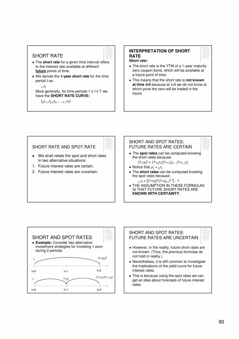
80
SHORT RATE
� The short rate for a given time interval refers
to the interest rate available at different future points of time.
� We denote the 1-year short rate for the time
period t as:
t-1rt
More generally, for time periods 1 ≤ t ≤ T we
have the SHORT RATE CURVE:
{0r1,1r2,2r3,….,T-1rT}
INTERPRETATION OF SHORT RATEShort rate:
� The short rate is the YTM of a 1-year maturity zero coupon bond, which will be available at
a future point of time.
� This means that the short rate is not known at time t=0 because at t=0 we do not know at which price the zero will be traded in the
future.
SHORT RATE AND SPOT RATE
� We shall relate the spot and short rates in two alternative situations:
1. Future interest rates are certain.
2. Future interest rates are uncertain.
SHORT AND SPOT RATES:FUTURE RATES ARE CERTAIN
� The spot rates can be computed knowing the short rates because:
(1+yt)t = (1+0r1)(1+1r2)…(1+t-1rt)
� Notice that y1 = 0r1.
� The short rates can be computed knowing the spot rates because:
t-1rt = [(1+yt)t/(1+yt-1)
t-1] - 1
� THE ASSUMPTION IN THESE FORMULAS IS THAT FUTURE SHORT RATES ARE KNOWN WITH CERTAINTY.
SHORT AND SPOT RATES� Example: Consider two alternative
investment strategies for investing 1 euro during 2 periods:
t=0 t=1 t=2
t=0 t=1 t=2
1
1
(1+y2)2
(1+y1)(1+1r2)1+y1
SHORT AND SPOT RATES:FUTURE RATES ARE UNCERTAIN
� However, in the reality, future short rates are not known. (Thus, the previous formulas do not hold in reality.)
� Nevertheless, it is still common to investigate
the implications of the yield curve for future interest rates:
� This is because using the spot rates we can
get an idea about forecasts of future interest rates.
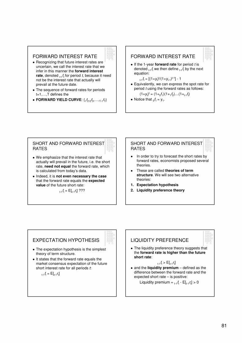
81
FORWARD INTEREST RATE� Recognizing that future interest rates are
uncertain, we call the interest rate that we infer in this manner the forward interest rate, denoted t-1ft for period t, because it need
not be the interest rate that actually will prevail at the future date.
� The sequence of forward rates for periods
t=1,…,T defines the
� FORWARD YIELD CURVE: {1f2,2f3,…,T-1fT}
FORWARD INTEREST RATE
� If the 1-year forward rate for period t is denoted t-1ft we then define t-1ft by the next
equation:
t-1ft = [(1+yt)t/(1+yt-1)
t-1] - 1
� Equivalently, we can express the spot rate for
period t using the forward rates as follows:
(1+yt)t = (1+0f1)(1+1f2)…(1+t-1ft)
� Notice that 0f1 = y1.
SHORT AND FORWARD INTEREST RATES
� We emphasize that the interest rate that actually will prevail in the future, i.e. the short
rate, need not equal the forward rate, which is calculated from today’s data.
� Indeed, it is not even necessary the casethat the forward rate equals the expected value of the future short rate:
t-1ft = E[t-1rt] ???
SHORT AND FORWARD INTEREST RATES
� In order to try to forecast the short rates by forward rates, economists proposed several
theories.
� These are called theories of term structure. We will see two alternative theories:
1. Expectation hypothesis
2. Liquidity preference theory
EXPECTATION HYPOTHESIS
� The expectation hypothesis is the simplest theory of term structure.
� It states that the forward rate equals the market consensus expectation of the future
short interest rate for all periods t:
t-1ft = E[t-1rt]
LIQUIDITY PREFERENCE
� The liquidity preference theory suggests that the forward rate is higher than the future short rate:
t-1ft > E[t-1rt]
� and the liquidity premium – defined as the
difference between the forward rate and the expected short rate – is positive:
Liquidity premium = t-1ft - E[t-1rt] > 0
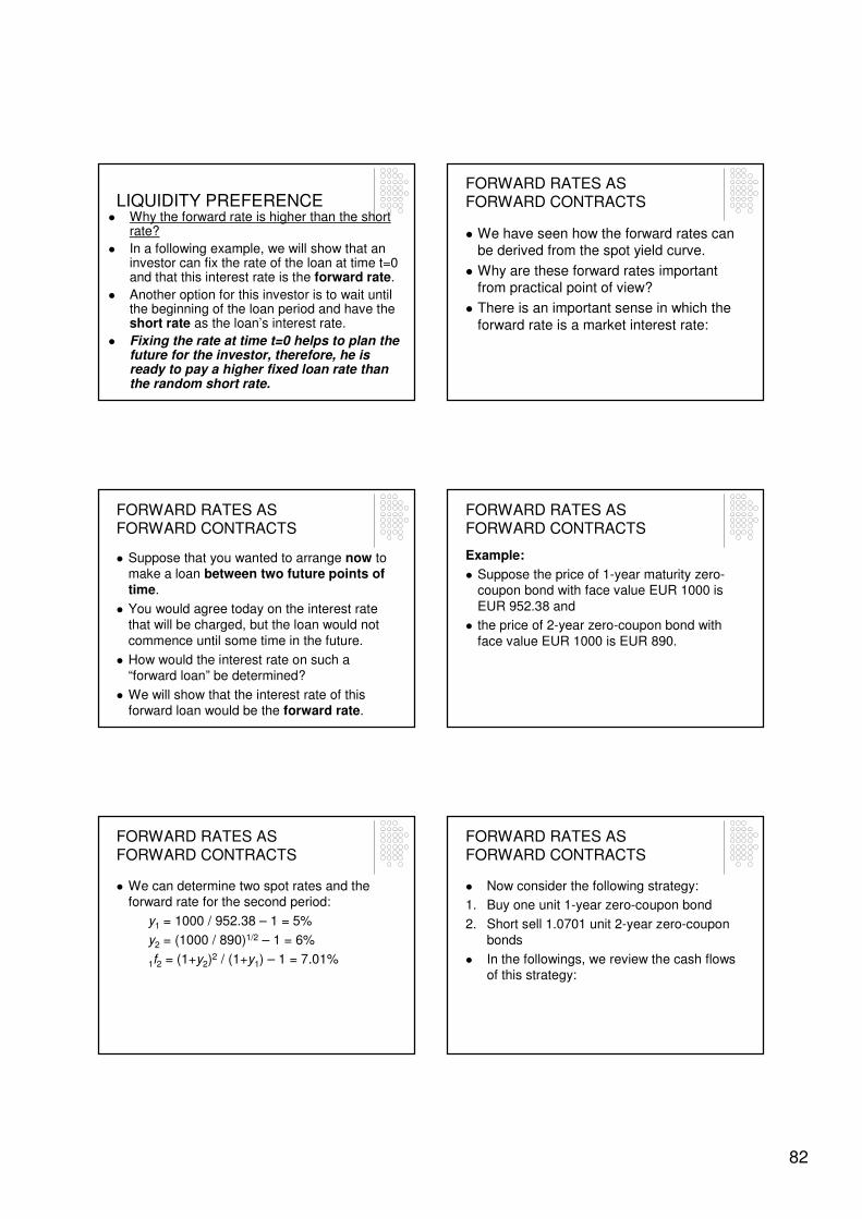
82
LIQUIDITY PREFERENCE� Why the forward rate is higher than the short
rate?
� In a following example, we will show that an investor can fix the rate of the loan at time t=0 and that this interest rate is the forward rate.
� Another option for this investor is to wait until the beginning of the loan period and have the short rate as the loan’s interest rate.
� Fixing the rate at time t=0 helps to plan the future for the investor, therefore, he is ready to pay a higher fixed loan rate than the random short rate.
FORWARD RATES AS FORWARD CONTRACTS
� We have seen how the forward rates can be derived from the spot yield curve.
� Why are these forward rates important from practical point of view?
� There is an important sense in which the
forward rate is a market interest rate:
FORWARD RATES AS FORWARD CONTRACTS
� Suppose that you wanted to arrange now to make a loan between two future points of time.
� You would agree today on the interest rate that will be charged, but the loan would not
commence until some time in the future.
� How would the interest rate on such a “forward loan” be determined?
� We will show that the interest rate of this forward loan would be the forward rate.
FORWARD RATES AS FORWARD CONTRACTS
Example:
� Suppose the price of 1-year maturity zero-coupon bond with face value EUR 1000 is
EUR 952.38 and
� the price of 2-year zero-coupon bond with
face value EUR 1000 is EUR 890.
FORWARD RATES AS FORWARD CONTRACTS
� We can determine two spot rates and the forward rate for the second period:
y1 = 1000 / 952.38 – 1 = 5%
y2 = (1000 / 890)1/2 – 1 = 6%
1f2 = (1+y2)2 / (1+y1) – 1 = 7.01%
FORWARD RATES AS FORWARD CONTRACTS
� Now consider the following strategy:
1. Buy one unit 1-year zero-coupon bond
2. Short sell 1.0701 unit 2-year zero-coupon
bonds
� In the followings, we review the cash flows of this strategy:
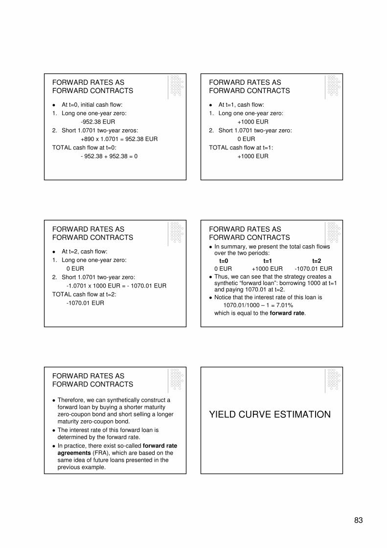
83
FORWARD RATES AS FORWARD CONTRACTS
� At t=0, initial cash flow:
1. Long one one-year zero:
-952.38 EUR
2. Short 1.0701 two-year zeros:
+890 x 1.0701 = 952.38 EUR
TOTAL cash flow at t=0:
- 952.38 + 952.38 = 0
FORWARD RATES AS FORWARD CONTRACTS
� At t=1, cash flow:
1. Long one one-year zero:
+1000 EUR
2. Short 1.0701 two-year zero:
0 EUR
TOTAL cash flow at t=1:
+1000 EUR
FORWARD RATES AS FORWARD CONTRACTS
� At t=2, cash flow:
1. Long one one-year zero:
0 EUR
2. Short 1.0701 two-year zero:
-1.0701 x 1000 EUR = - 1070.01 EUR
TOTAL cash flow at t=2:
-1070.01 EUR
FORWARD RATES AS FORWARD CONTRACTS
� In summary, we present the total cash flows over the two periods:
t=0 t=1 t=2
0 EUR +1000 EUR -1070.01 EUR
� Thus, we can see that the strategy creates a synthetic “forward loan”: borrowing 1000 at t=1 and paying 1070.01 at t=2.
� Notice that the interest rate of this loan is
1070.01/1000 – 1 = 7.01%
which is equal to the forward rate.
FORWARD RATES AS FORWARD CONTRACTS
� Therefore, we can synthetically construct a forward loan by buying a shorter maturity zero-coupon bond and short selling a longer
maturity zero-coupon bond.
� The interest rate of this forward loan is determined by the forward rate.
� In practice, there exist so-called forward rate agreements (FRA), which are based on the same idea of future loans presented in the previous example.
YIELD CURVE ESTIMATION
84
ESTIMATING THE YIELD CURVE
� We talked about how can we use the values of the spot yield curve in order to discount
future cash flows.
� However, in the reality we do not observe the yield curve.
� In the real world, we observe:
1. The bid and asked prices of bonds
2. The cash flows of coupon and par value payments of bonds.
ESTIMATING THE YIELD CURVE� It is useful from a practical point of view to
estimate the spot yield curve because it helps us to discount cash flows paid at any time in the future.
� Therefore, given the yield curve we can price
any fixed-income financial asset on the market.
ESTIMATING THE YIELD CURVE
� In this section, we review a methodology to estimate the spot yield curve given the
observed bond prices and future cash flow payments.
ESTIMATING THE YIELD CURVE
� We will start with observed data on (1) bid and asked prices, (2) accrued interest and (3)
future cash flows of several bonds traded on the market.
� We also know the exact day of each cash flow payment.
� In order to estimate the spot yield curve, we
proceed as follows:
ESTIMATING THE YIELD CURVE
1. Compute the market price, p for each bond by the next formula:
p = (Asked price + Bid price)/2
+ Accrued interest
ESTIMATING THE YIELD CURVE
2. To get an estimate of the spot rate, yt use
the following cubic polynomialapproximation of the log-spot rate, yt:
ln yt = a + bt + ct2 + dt3
where a, b, c and d are the parameters of the cubic polynomial.
� Remark 1: We approximate the log-interest
rate because we want to avoid sign restrictions on the a, b, c and d parameters
(as yt is positive).
85
ESTIMATING THE YIELD CURVE
� Remark 2: We employ a cubic polynomial approximation because a third-order
polynomial can model the yield curve in a very flexible way:
� It can capture various types of increasing / decreasing / convex / concave parts of the
yield curve.
� Therefore, the model can be very realistic.
ESTIMATING THE YIELD CURVE
� In the followings, first, we assume that the parameter values a, b, c, d are given and we
present how to value of the bonds given these parameters estimates.
� Later, we shall discuss how can we estimate the parameters.
ESTIMATING THE YIELD CURVE
3. Given the parameters, we compute the value of yt by taking the exponential of the cubic
polynomial of ln yt.
4. Then, we compute the discount factor for each point of time t according to the next formula:
ESTIMATING THE YIELD CURVE
5. Afterwards, we use the discount factors to compute the present value of future cash flows: PV(CFt) = CFt x DF(t,yt)
6. Then, we sum these present values to get an estimate of the bond price:
where p* is the bond price estimate, PV denotes present value.
ESTIMATING THE YIELD CURVE
7. Finally, we compute the following measure of estimation precision:
where MSE is the mean squared error, N is the number of bonds observed, pi is the
observed market price of the i-th bond and pi*is the estimate of the i-th bond price.
ESTIMATING THE YIELD CURVE
� How do we choose the values of the parameters?
� We choose parameter values such that the
MSE precision measure is minimized.
� The MSE minimization can be done
numerically in Excel using the SOLVER tool.
� (In Excel use: Tools / Solver or Herramientas/ Solver.)
86
MANAGING BOND
PORTFOLIOS
MANAGING BOND PORTFOLIOS
� We are going to review several topics related to bond portfolio management.
� In particular, we shall see:
1. Evolution of bond prices over time
2. Interest rate risk of bonds
3. Default or credit risk of bonds
EVOLUTION OF
BOND PRICES OVER TIME
EVOLUTION OF BOND PRICES OVER TIME
� In this section we are going to be in a
dynamic framework.
� That is we shall analyze the evolution of the bond price over several periods:
� t=0,1,2,…,T.
EVOLUTION OF BOND PRICES OVER TIME
� As we have discussed before, the determinants of bond value are:
1. Future cash flow payments (i.e., coupon
payments + par value payments)
2. Time to maturity,
3. Values of the yield-to-maturity (YTM) or
spot yield curve used to discount these cash flows.
EVOLUTION OF BOND PRICES OVER TIME
� We shall investigate the evolution of bond price under two alternative situations:
1.The YTM is constant over time (NOT
REALISTIC ASSUMPTION but it helps to understand a basic characteristic of the bond price evolution.)
2.The YTM changes over time (MORE
REALISTIC SETUP)
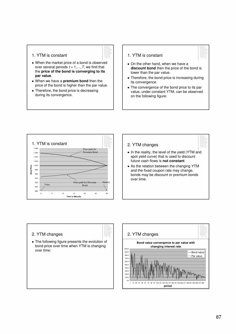
87
1. YTM is constant
� When the market price of a bond is observed over several periods t = 1,…,T, we find that
the price of the bond is converging to its par value.
� When we have a premium bond then the price of the bond is higher than the par value.
� Therefore, the bond price is decreasing
during its convergence.
1. YTM is constant
� On the other hand, when we have a discount bond then the price of the bond is
lower than the par value.
� Therefore, the bond price is increasing during
its convergence.
� The convergence of the bond price to its par value, under constant YTM, can be observed
on the following figure:
1. YTM is constant
880
900
920
940
960
980
1,000
1,020
1,040
1,060
1,080
0 5 10 15 20 25 30
Time to Maturity
Bo
nd
Pri
ce
Price path for
Premium Bond
Price path for Discount
BondTodayMaturity
2. YTM changes
� In the reality, the level of the yield (YTM and spot yield curve) that is used to discount
future cash flows is not constant.
� As the relation between the changing YTM and the fixed coupon rate may change, bonds may be discount or premium bonds
over time.
2. YTM changes
� The following figure presents the evolution of bond price over time when YTM is changing
over time:
2. YTM changes
Bond value convergence to par value with
changing interest rate
0.0
100.0
200.0
300.0
400.0
500.0
600.0
700.0
800.0
900.0
1000.0
1 13 25 37 49 61 73 85 97 109 121 133 145 157 169 181 193 205 217 229 241 253 265 277 289
period
Bond value
Par value
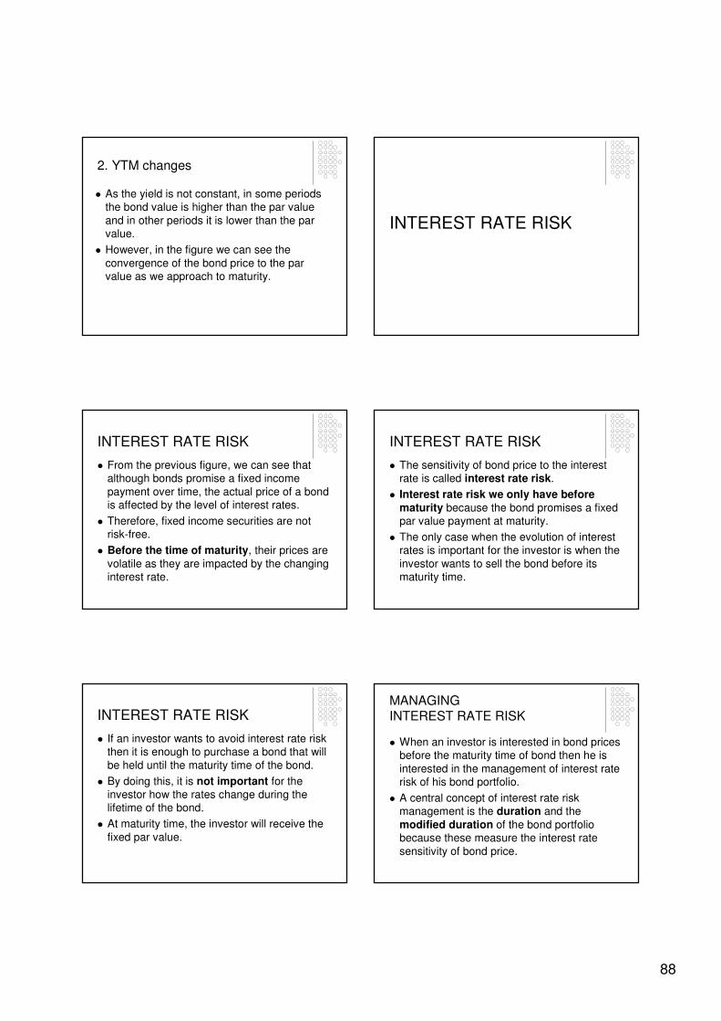
88
2. YTM changes
� As the yield is not constant, in some periods the bond value is higher than the par value
and in other periods it is lower than the par value.
� However, in the figure we can see the
convergence of the bond price to the par value as we approach to maturity.
INTEREST RATE RISK
INTEREST RATE RISK
� From the previous figure, we can see that although bonds promise a fixed income
payment over time, the actual price of a bond is affected by the level of interest rates.
� Therefore, fixed income securities are not risk-free.
� Before the time of maturity, their prices are
volatile as they are impacted by the changing interest rate.
INTEREST RATE RISK
� The sensitivity of bond price to the interest rate is called interest rate risk.
� Interest rate risk we only have before maturity because the bond promises a fixed par value payment at maturity.
� The only case when the evolution of interest rates is important for the investor is when the
investor wants to sell the bond before its maturity time.
INTEREST RATE RISK
� If an investor wants to avoid interest rate risk then it is enough to purchase a bond that will
be held until the maturity time of the bond.
� By doing this, it is not important for the investor how the rates change during the lifetime of the bond.
� At maturity time, the investor will receive the
fixed par value.
MANAGING INTEREST RATE RISK
� When an investor is interested in bond prices before the maturity time of bond then he is
interested in the management of interest rate risk of his bond portfolio.
� A central concept of interest rate risk management is the duration and the
modified duration of the bond portfolio because these measure the interest rate
sensitivity of bond price.
89
DURATION
� The duration is the weighted average of the
times of each coupon payment where the weights, wt are
where y is the YTM of the bond and durationis computed as
DURATION
� The duration can be interpreted as the effective average maturity of the bond
portfolio.
� The scale of the duration is years.
DURATION of specific bonds
(1) The duration of a zero-coupon bond is
equal to the maturity of the zero-coupon bond: D=T.
(2) The duration of a T-year annual annuity is:
D=(1+y)/y – T / [(1+y)T – 1]
(3) The duration of an annual perpetuity is
D=(1+y)/y
where y denotes yield in (2) and (3).
MODIFIED DURATION
� The modified duration for any bond is defined as
where y is the annual YTM of the bond.
MODIFIED DURATION
• Modified duration can be used to compute
the interest rate sensitivity of bond prices because:
where P is the bond price, y is the annual YTM of the bond.
MODIFIED DURATION
� The modified duration also helps to answer the following more practical question:
� Question: What is the percentage change of the bond price when the interest rate changes by ∆y?
� Answer: When the interest rate change is relatively small than the percentage price change is approximately:
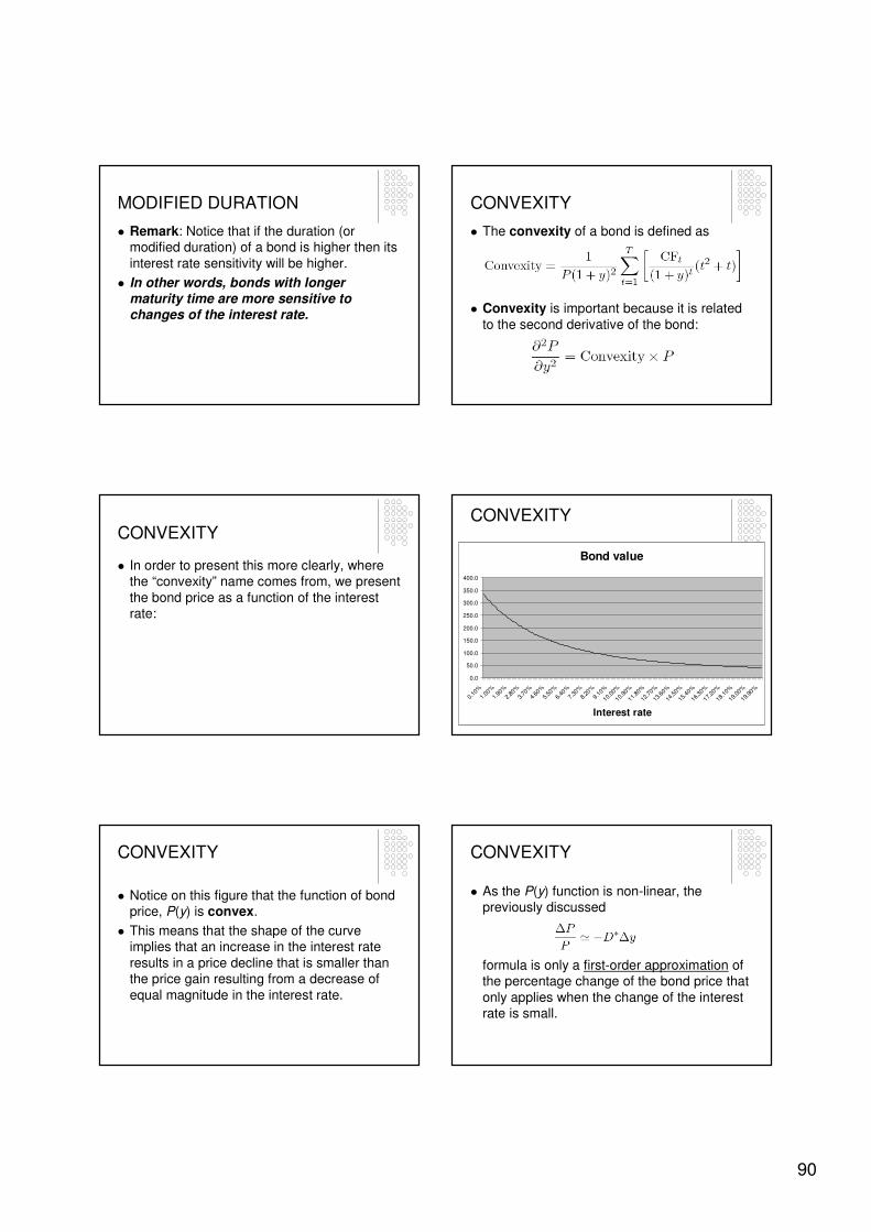
90
MODIFIED DURATION
� Remark: Notice that if the duration (or modified duration) of a bond is higher then its
interest rate sensitivity will be higher.
� In other words, bonds with longer maturity time are more sensitive to changes of the interest rate.
CONVEXITY
� The convexity of a bond is defined as
� Convexity is important because it is related
to the second derivative of the bond:
CONVEXITY
� In order to present this more clearly, where the “convexity” name comes from, we present
the bond price as a function of the interest rate:
CONVEXITY
Bond value
0.0
50.0
100.0
150.0
200.0
250.0
300.0
350.0
400.0
0.10
%
1.00
%
1.90
%
2.80
%
3.70
%
4.60
%
5.50
%
6.40
%
7.30
%
8.20
%
9.10
%
10.0
0%
10.9
0%
11.8
0%
12.7
0%
13.6
0%
14.5
0%
15.4
0%
16.3
0%
17.2
0%
18.1
0%
19.0
0%
19.9
0%
Interest rate
CONVEXITY
� Notice on this figure that the function of bond price, P(y) is convex.
� This means that the shape of the curve implies that an increase in the interest rate
results in a price decline that is smaller than the price gain resulting from a decrease of
equal magnitude in the interest rate.
CONVEXITY
� As the P(y) function is non-linear, the previously discussed
formula is only a first-order approximation of the percentage change of the bond price that
only applies when the change of the interest rate is small.
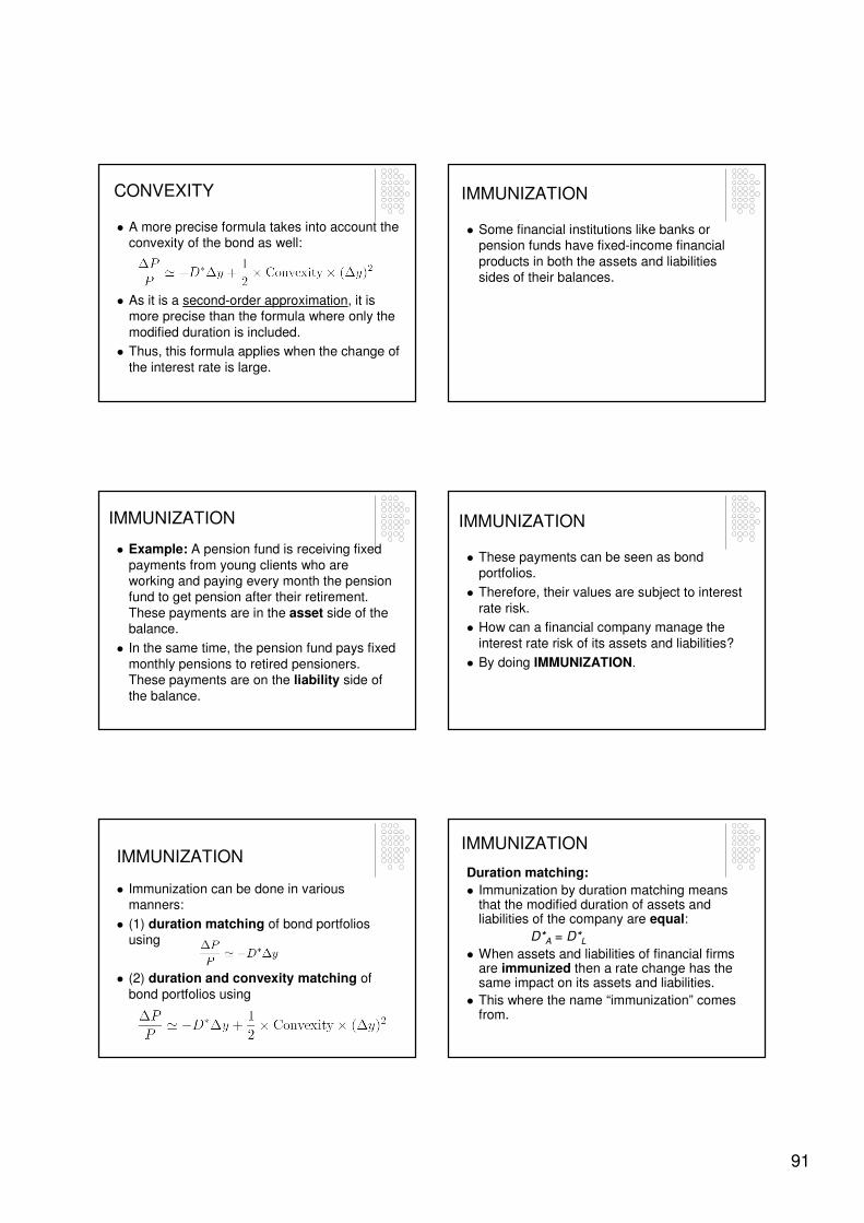
91
CONVEXITY
� A more precise formula takes into account the convexity of the bond as well:
� As it is a second-order approximation, it is more precise than the formula where only the
modified duration is included.
� Thus, this formula applies when the change of
the interest rate is large.
IMMUNIZATION
� Some financial institutions like banks or pension funds have fixed-income financial
products in both the assets and liabilities sides of their balances.
IMMUNIZATION
� Example: A pension fund is receiving fixed
payments from young clients who are working and paying every month the pension fund to get pension after their retirement.
These payments are in the asset side of the balance.
� In the same time, the pension fund pays fixed
monthly pensions to retired pensioners. These payments are on the liability side of
the balance.
IMMUNIZATION
� These payments can be seen as bond portfolios.
� Therefore, their values are subject to interest
rate risk.
� How can a financial company manage the
interest rate risk of its assets and liabilities?
� By doing IMMUNIZATION.
IMMUNIZATION
� Immunization can be done in various manners:
� (1) duration matching of bond portfolios using
� (2) duration and convexity matching of
bond portfolios using
IMMUNIZATION
Duration matching:
� Immunization by duration matching means that the modified duration of assets and liabilities of the company are equal:
D*A = D*L
� When assets and liabilities of financial firms are immunized then a rate change has the same impact on its assets and liabilities.
� This where the name “immunization” comes from.
92
IMMUNIZATION
Duration and convexity matching:
� Immunization by duration and convexity
matching means that the modified duration and convexity of assets and liabilities of the
company are equal:
D*A = D*L
and
ConvexityA = ConvexityL
IMMUNIZATION
Conclusion on immunization:
� The duration and convexity matching immunizes better for large movements in the interest rate than the more simple duration matching.
� However, the determination of the immunizing bond portfolio may be complicated.
� When the more simple, duration matching is considered, the manager can hedge for relatively small changes in the yield.
DEFAULT OF BONDS:
CREDIT RISK
Default risk
� Although bonds generally promise a fixed flow of income, that income stream is not
risk-free unless the issuer will not default on the obligation.
� While most government bonds may be treated as assets free of default risk, this is
not true for corporate bonds.
Default risk
� Bond default risk, usually called credit risk, is measured by the next firms:
1. Moody’s,
2. Standard and Poor’s (S&P’s) and
3. Fitch
These institutions provide financial information on firms as well as quality
ratings of large corporate and municipal bond issues.
Default risk
� International bonds, especially in emerging markets, also are commonly rated for default
risk.
� Each rating firm assigns letter grades to the bonds to reflect their assessment of the safety of the bond issue.
� In the following table, the grades of Moody’s
and Standard and Poor’s are presented:

93
Default risk
Speculative-grade / Junk bondVery poorDD
Speculative-grade / Junk bondVery poorCC
Speculative-grade / Junk bondVery poorCCCa
Speculative-grade / Junk bondVery poorCCCCaa
Speculative-grade / Junk bondSpeculativeBB
Speculative-grade / Junk bondSpeculativeBBBa
Investment-grade bondHigh qualityBBBBaa
Investment-grade bondHigh qualityAA
Investment-grade bondVery high qualityAAAa
Investment-grade bondVery high qualityAAAAaa
Bond gradeQuality of bond
S&P's
rating
Moody's
rating
Default risk
� At times Moody’s and S&P’s use adjustments to these ratings:
1. S&P uses plus and minus signs: A+ is the strongest and A- is the weakest.
2. Moody’s uses a 1, 2 or 3 designation, with
A1 indicating the strongest and A3 indicating the weakest.
Determinants of bond safety
� Rating agencies base their quality ratings largely on the level and trend of issuer’s
financial ratios.
� The key ratios are:
1. Coverage ratios: Ratios of company
earnings to fixed costs.
2. Leverage ratio: Debt-to-equity ratio.
Determinants of bond safety
3. Liquidity ratios:
3a. Current ratio =
Current assets / current liabilities
3b. Quick ratio =
Current assets excluding inventories /
current liabilities
Determinants of bond safety
4. Profitability ratios: Measures of rates of return on assets or equity
4a. Return on assets (ROA) =
Net income / total assets
4b. Return on equity (ROE) =
Net income / equity
5. Cash flow-to-debt ratio: Ratio of total cash flow to outstanding debt
Default premium
� To compensate for the possibility of default, corporate bonds must offer a default premium.
� The default premium is the difference
between the promised yield to maturity on a corporate bond and the yield to maturity of an
otherwise identical government bond that is risk-free in terms of default.
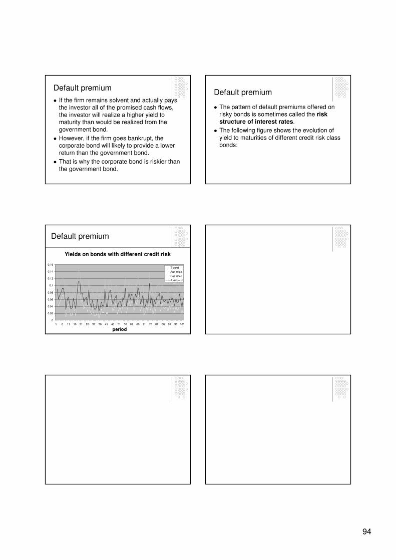
94
Default premium
� If the firm remains solvent and actually pays the investor all of the promised cash flows,
the investor will realize a higher yield to maturity than would be realized from the
government bond.
� However, if the firm goes bankrupt, the corporate bond will likely to provide a lower return than the government bond.
� That is why the corporate bond is riskier than
the government bond.
Default premium
� The pattern of default premiums offered on risky bonds is sometimes called the risk structure of interest rates.
� The following figure shows the evolution of
yield to maturities of different credit risk class bonds:
Default premium
Yields on bonds with different credit risk
0
0.02
0.04
0.06
0.08
0.1
0.12
0.14
0.16
1 6 11 16 21 26 31 36 41 46 51 56 61 66 71 76 81 86 91 96 101
period
T-bond
Aaa rated
Baa rated
Junk bond
95
DERIVATIVES
DERIVATIVES
A derivative is a financial instrument that is derived from some other asset (known as
the underlying asset).
Rather than trade or exchange the underlying asset itself, derivative traders enter into an agreement that involves a final payoff which
depends on the price of the underlying asset.
A GENERAL DEFINITION OF DERIVATIVES
� The final payoff of a derivative is always a specific function of past and current prices of
the underlying asset.
(Payoff of derivative at time t) = f (S1,…,St)
where St is the price of the underlying asset
at time t and f (·) is the payoff function of the derivative.
A GENERAL DEFINITION OF RELATIVELY SIMPLE DERIVATIVES
� The payoff of the more simple derivatives depends only on the current price of the
underlying asset:
(Payoff of derivative at time t) = f (St)
� Most derivatives that we see in this course
have this type of payoff function.
A REMARK
� The word “derivative” has nothing to do with the derivative that you have studied in
differentiation during the mathematical calculus course.
� The word “derivative” refers to the fact that the payoff of a derivative is a function of the price
of the underlying asset.
� The payoff function defines the derivative.
� Different derivatives have different payoff functions.
DERIVATIVES
� Important types of derivatives are:
1. FUTURES and FORWARDS
2. OPTIONS
3. SWAPS

96
FUTURES
FUTURES
� A contract to buy or sell an asset on a future date at a fixed price.
� The buyer and the seller of the futures
contract have the obligation to buy or sell the asset.
FUTURES
� The buyer of the futures contract is in long futures position.
� The seller of the futures contract is in short futures position.
FUTURES
� The underlying asset of the futures contract can be:
1. Commodity like grain, metals or energy
2. Financial product like interest rate, exchange rate, stock or stock index
ELEMENTS OF FUTURES CONTRACT
� The main elements of the futures contract are the
1. Futures price, F
This is the price fixed in the contract at which the transaction will occur in the future.
2. Expiration date, T
This is the date fixed in the contract when
the delivery will take place in the future.
PAYOFF OF FUTURES CONTRACT
� The payoff and the profit of the long futuresposition at the expiration date, T is
Payoff = Profit = ST – F
where ST is the price of the underlying product at time T.
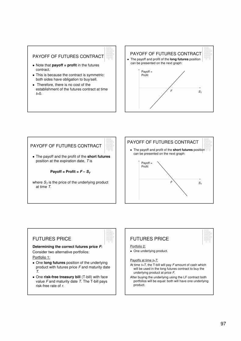
97
PAYOFF OF FUTURES CONTRACT
� Note that payoff = profit in the futures contract.
� This is because the contract is symmetric: both sides have obligation to buy/sell.
� Therefore, there is no cost of the
establishment of the futures contract at time t=0.
PAYOFF OF FUTURES CONTRACT� The payoff and profit of the long futures position
can be presented on the next graph:
F ST
Payoff = Profit
PAYOFF OF FUTURES CONTRACT
� The payoff and the profit of the short futuresposition at the expiration date, T is
Payoff = Profit = F – ST
where ST is the price of the underlying product at time T.
PAYOFF OF FUTURES CONTRACT
� The payoff and profit of the short futures position can be presented on the next graph:
Payoff = Profit
STF
FUTURES PRICE
Determining the correct futures price F:
Consider two alternative portfolios:
Portfolio 1:
� One long futures position of the underlying
product with futures price F and maturity date T.
� One risk-free treasury bill (T-bill) with face
value F and maturity date T. The T-bill pays risk-free rate of r.
FUTURES PRICE
Portfolio 2:
� One underlying product.
Payoffs at time t=T:
At time t=T, the T-bill will pay F amount of cash which will be used in the long futures contract to buy the
underlying product at price F.
After buying the underlying using the LF contract both portfolios will be equal: both will have one underlying
product.
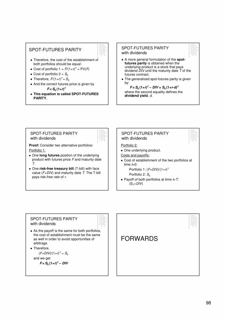
98
SPOT-FUTURES PARITY
� Therefore, the cost of the establishment of both portfolios should be equal:
� Cost of portfolio 1 = F/(1+r)T = PV(F)
� Cost of portfolio 2 = S0
� Therefore, F/(1+r)T = S0
� And the correct futures price is given by
F = S0 (1+r)T
� This equation is called SPOT-FUTURES PARITY.
SPOT-FUTURES PARITY with dividends
� A more general formulation of the spot-futures parity is obtained when the underlying product is a stock that pays dividend DIV until the maturity date T of the futures contract.
� The generalized spot-futures parity is given by:
F = S0 (1+r)T – DIV = S0 (1+r-d)T
where the second equality defines the dividend yield, d.
SPOT-FUTURES PARITY with dividends
Proof: Consider two alternative portfolios:
Portfolio 1:
� One long futures position of the underlying product with futures price F and maturity date T.
� One risk-free treasury bill (T-bill) with face
value (F+DIV) and maturity date T. The T-bill pays risk-free rate of r.
SPOT-FUTURES PARITY with dividends
Portfolio 2:
� One underlying product.
Costs and payoffs:
� Cost of establishment of the two portfolios at
time t=0:
Portfolio 1: (F+DIV)/(1+r)T
Portfolio 2: S0
� Payoff of both portfolios at time t=T:
(ST+DIV)
SPOT-FUTURES PARITY with dividends
� As the payoff is the same for both portfolios, the cost of establishment must be the same
as well in order to avoid opportunities of arbitrage.
� Therefore,
(F+DIV)/(1+r)T = S0
and we get
F = S0 (1+r)T – DIV
FORWARDS

99
FUTURES AND FORWARDS
� Forward contracts are the same as futures contracts:
� Both are about buying or selling an asset on
a future date at a fixed price.
� In both, the buyer and the seller have the
obligation to buy or sell the asset.
� Also the underlying asset of both contract can be either commodity or another financial
asset.
FUTURES AND FORWARDS
� The distinction between “futures” and “forward” does not apply to the contract, but
to how the contract is traded.
Trading of futures contracts
� Futures contracts are always traded in organized exchanges.
� In an organized exchange, futures products
are standardized (with respect to possible maturity times and quality of products) and this way the liquidity of the futures market
is increased.
Trading of futures contracts
� As futures products are standardized, it is possible that the quality and prices of “local”
commodity product that the investor wants to hedge using a commodity futures contract is
not the same as the quality and price of the underlying commodity of the futures contract
traded at the organized exchange.
Trading of futures contracts
� Although there is a common dependence between local and exchange prices and
quality (i.e. there is a high correlation), the correlation is not perfect.
� In risk management, this type of risk is called basis risk.
Trading of futures contracts
� Another consequence of standardized futures commodity exchanges is that the geographic
location of the futures exchange may be far from the investor’s location.
� This can make costly and inconvenient the physical delivery of the commodity.
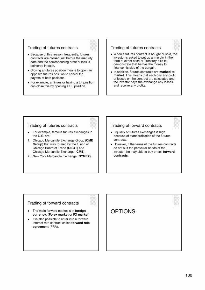
100
Trading of futures contracts
� Because of this reason, frequently, futures contracts are closed just before the maturity
date and the corresponding profit or loss is delivered in cash.
� Closing a futures position means to open an opposite futures position to cancel the
payoffs of both positions.
� For example, an investor having a LF position can close this by opening a SF position.
Trading of futures contracts
� When a futures contract is bought or sold, the investor is asked to put up a margin in the form of either cash or Treasury-bills to demonstrate that he has the money to finance his side of the bargain.
� In addition, futures contracts are marked-to-market. This means that each day any profit or losses on the contract are calculated and the investor pays the exchange any losses and receive any profits.
Trading of futures contracts
� For example, famous futures exchanges in the U.S. are:
1. Chicago Mercantile Exchange Group (CME Group) that was formed by the fusion of Chicago Board of Trade (CBOT) and Chicago Mercantile Exchange (CME).
2. New York Mercantile Exchange (NYMEX).
Trading of forward contracts
� Liquidity of futures exchanges is high because of standardization of the futures
contracts.
� However, if the terms of the futures contracts do not suit the particular needs of the investor, he may able to buy or sell forward contracts.
Trading of forward contracts
� The main forward market is in foreign currency. (Forex market or FX market)
� It is also possible to enter into a forward interest rate contract called forward rate agreement (FRA).
OPTIONS

101
OPTIONS
� An option is a contract between a buyer and a seller that gives the buyer the right - but not
the obligation - to buy or to sell a particular asset (the underlying asset) at a later day at
an agreed strike price.
� The purchase price of the option is called the
premium. It represents the compensation the purchaser of the call must pay for the right to
exercise the option.
OPTIONS
� Sellers of options, who are said to writeoptions, receive premium income at the
moment when the options contract is signed as payment against the possibility they will be required at some later date to deliver the
asset in return for an exercise price or strike price.
CALL AND PUT OPTIONS
� A call option gives the buyer the right to buythe underlying asset.
� A put option gives the buyer of the option
the right to sell the underlying asset.
� If the buyer chooses to exercise this right, the
seller is obliged to sell or buy the asset at the agreed price.
� The buyer may choose not to exercise the
right and let it expire.
OPTIONS POSITIONS
� The buyer of the call option is in long call (LC) position.
� The seller of the call option is in short call (SC) position.
� The buyer of the put option is in long put (LP) position.
� The seller of the put option is in short put (SP) position.
ELEMENTS OF OPTIONS CONTRACT
� The main elements of the options contract are the
1. Strike price, X
This is the price fixed in the contract at which the buyer of the option can exercise his right to buy or
sell the underlying product.
2. Expiration date, T
This is the future date fixed in the contract until which the buyer can exercise his option.
EUROPEAN / AMERICAN OPTIONS
� There are two types of options:
1. European option:
The buyer of the option can exercise his right to buy or sell the underlying product only on the expiration date.
2. American option:
The buyer of the option can exercise his
right to buy or sell the underlying product at on or before the expiration date.
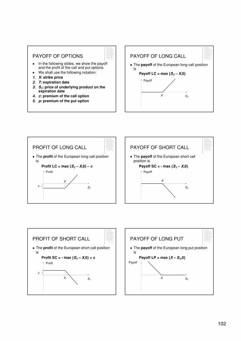
102
PAYOFF OF OPTIONS
� In the following slides, we show the payoff and the profit of the call and put options.
� We shall use the following notation:
1. X: strike price
2. T: expiration date
3. ST: price of underlying product on the expiration date
4. c: premium of the call option
5. p: premium of the put option
PAYOFF OF LONG CALL
� The payoff of the European long call position is
Payoff LC = max {ST – X,0}
Payoff
STX
PROFIT OF LONG CALL
� The profit of the European long call position is
Profit LC = max {ST – X,0} – c
Profit
X
STc
PAYOFF OF SHORT CALL
� The payoff of the European short call position is
Payoff SC = - max {ST – X,0}
Payoff
ST
X
PROFIT OF SHORT CALL
� The profit of the European short call position is
Profit SC = - max {ST – X,0} + c
STX
Profit
c
PAYOFF OF LONG PUT
� The payoff of the European long put position is
Payoff LP = max {X – ST,0}
Payoff
STX
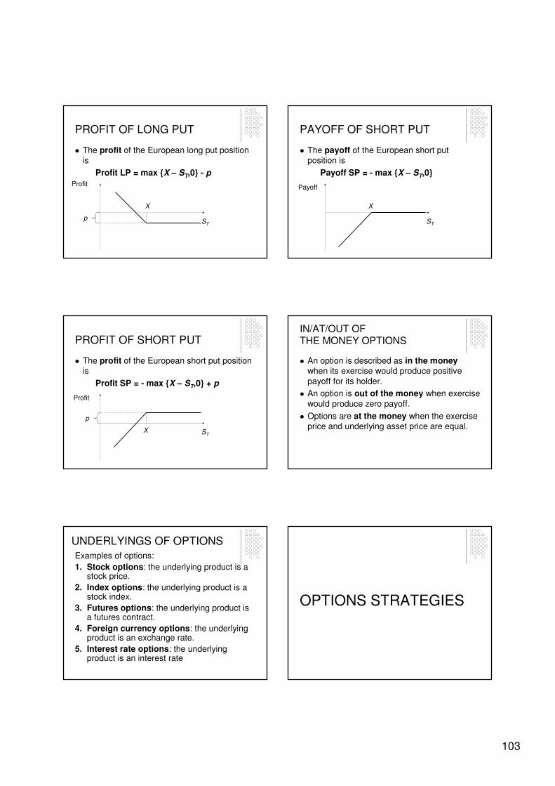
103
PROFIT OF LONG PUT
� The profit of the European long put position is
Profit LP = max {X – ST,0} - p
X
ST
Profit
p
PAYOFF OF SHORT PUT
� The payoff of the European short put position is
Payoff SP = - max {X – ST,0}
Payoff
ST
X
PROFIT OF SHORT PUT
� The profit of the European short put position is
Profit SP = - max {X – ST,0} + p
X ST
Profit
p
IN/AT/OUT OF THE MONEY OPTIONS
� An option is described as in the moneywhen its exercise would produce positive
payoff for its holder.
� An option is out of the money when exercise
would produce zero payoff.
� Options are at the money when the exercise price and underlying asset price are equal.
UNDERLYINGS OF OPTIONS
Examples of options:
1. Stock options: the underlying product is a stock price.
2. Index options: the underlying product is a stock index.
3. Futures options: the underlying product is a futures contract.
4. Foreign currency options: the underlying product is an exchange rate.
5. Interest rate options: the underlying product is an interest rate
OPTIONS STRATEGIES

104
OPTIONS STRATEGIES
Options trading strategies:
1. Call options trading strategy
2. Put options trading strategy
3. Protective put strategy
4. Covered call strategy
5. Straddle strategy
6. Spread strategy
CALL OPTION STRATEGY
Call options trading strategy:
� Purchasing call options (LC) provide profit when the price of the underlying product
increase.
� Selling call options (SC) provide profit when
the price of the underlying product decrease.
PUT OPTION STRATEGY
Put options trading strategy:
� Purchasing put options (LP) provide profit
when the price of the underlying product decrease.
� Selling put options (SP) provide profit when
the price of the underlying product increase.
PROTECTIVE PUT STRATEGY
� Protective put strategy:
1. Buying the underlying product (Long
Underlying) at price S0.
2. Buying a put option on the underlying product (LP) with strike price X.
PROTECTIVE PUT STRATEGY
1. Payoff of the long underlying position:
ST
Payoff
PROTECTIVE PUT STRATEGY
2. Payoff of the LP position:
Payoff
STX
X
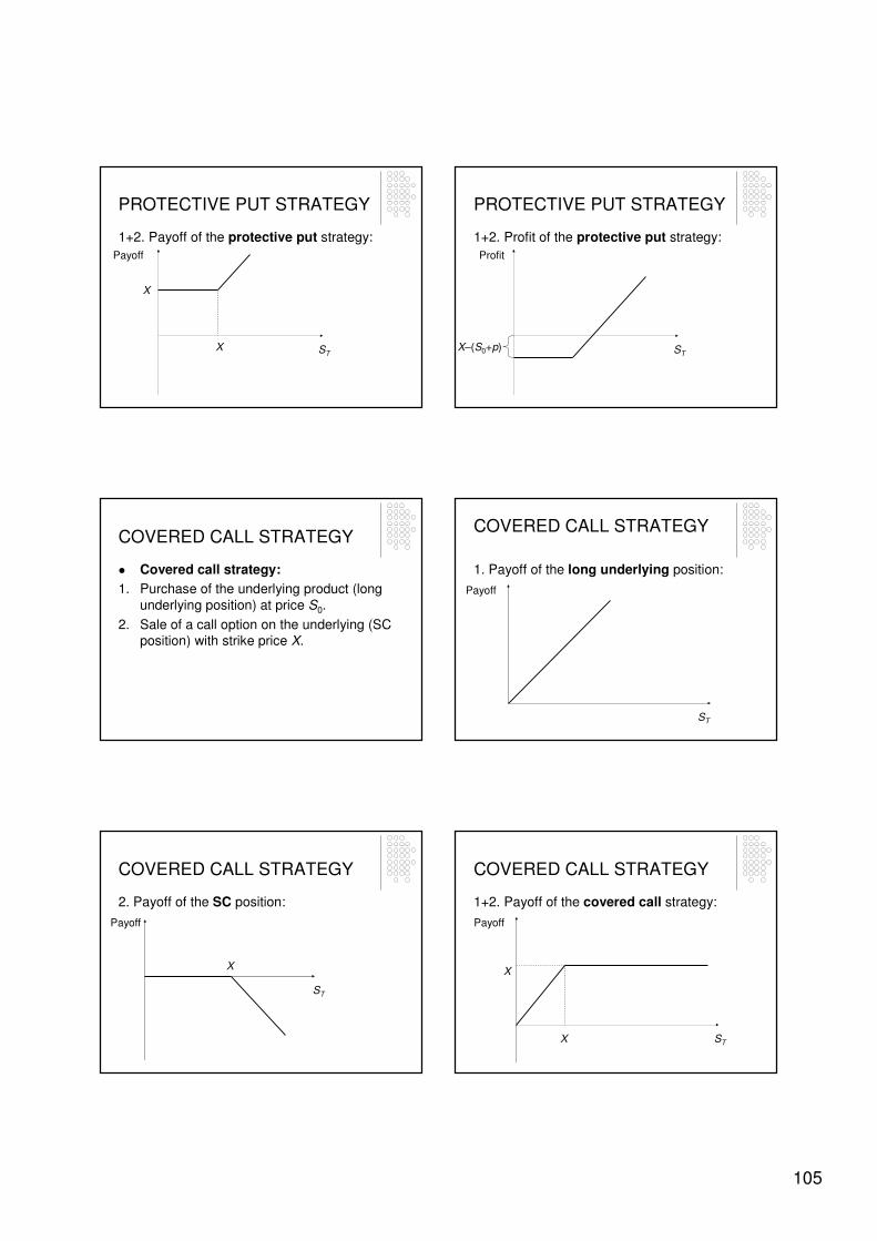
105
PROTECTIVE PUT STRATEGY
1+2. Payoff of the protective put strategy:
Payoff
STX
X
PROTECTIVE PUT STRATEGY
1+2. Profit of the protective put strategy:
ST
Profit
X–(S0+p)
COVERED CALL STRATEGY
� Covered call strategy:
1. Purchase of the underlying product (long
underlying position) at price S0.
2. Sale of a call option on the underlying (SC position) with strike price X.
COVERED CALL STRATEGY
1. Payoff of the long underlying position:
ST
Payoff
COVERED CALL STRATEGY
2. Payoff of the SC position:
X
Payoff
ST
COVERED CALL STRATEGY
1+2. Payoff of the covered call strategy:
X
X
ST
Payoff
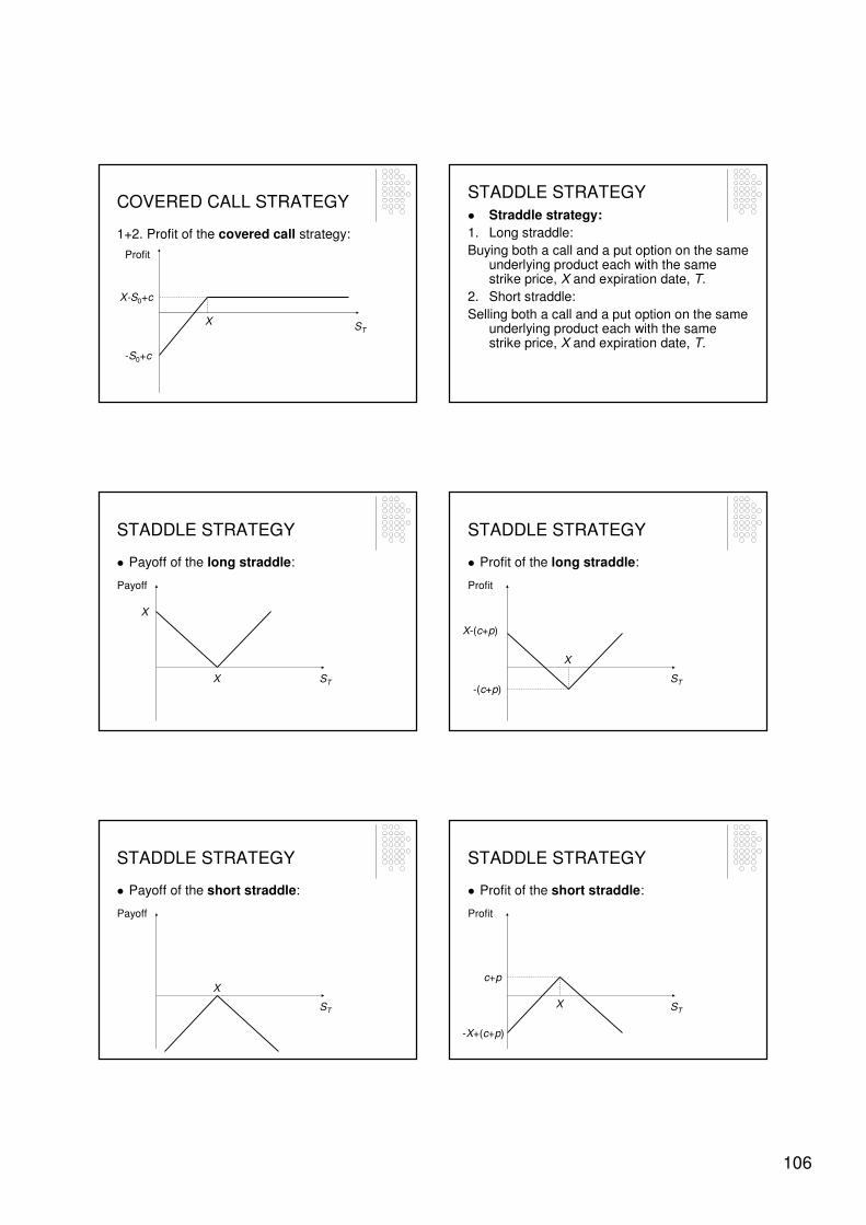
106
COVERED CALL STRATEGY
1+2. Profit of the covered call strategy:
ST
Profit
-S0+c
X-S0+c
X
STADDLE STRATEGY
� Straddle strategy:
1. Long straddle:
Buying both a call and a put option on the same underlying product each with the same strike price, X and expiration date, T.
2. Short straddle:
Selling both a call and a put option on the same underlying product each with the same strike price, X and expiration date, T.
STADDLE STRATEGY
� Payoff of the long straddle:
ST
Payoff
X
X
STADDLE STRATEGY
� Profit of the long straddle:
ST
X
X-(c+p)
-(c+p)
Profit
STADDLE STRATEGY
� Payoff of the short straddle:
Payoff
ST
X
STADDLE STRATEGY
� Profit of the short straddle:
ST
c+p
X
-X+(c+p)
Profit

107
STADDLE STRATEGY
Strip and strap strategies: These are variations of straddles.
1. Long strip: Buying two puts and one call with the
same strike price and exercise date.
2. Short strip: Selling two puts and one call with the same strike price and exercise date.
3. Long strap: Buying two calls and one put with the same strike price and exercise date.
4. Short strap: Selling two calls and one put with the
same strike price and exercise date.
SPREAD STRATEGY
� Spread strategy: A spread is a combination of two or more call options (or two or more put options) on the same underlying product with differing strike prices or expiration dates.
1. Money spread: involves the purchase and sale of options with different strike prices.
2. Time spread: involves the purchase and sale of options with different expiration dates.
SPREAD STRATEGY
� In the followings, we shall focus only on money spreads.
� We review three types of money spreads:
1. BULLISH SPREAD: used when the investor expects that the price of the underlying will increase.
2. BEARISH SPREAD: used when the investor expects that the price of the underlying will decrease.
3. BUTTERFLY SPREAD: used when the investor expects relatively small or relatively large price changes in the future.
SPREAD STRATEGY
� Bullish spread strategy: This can be constructed in two alternative ways:
1. First way:
(1a) Buying a call option with strike price X1
and
(1b) Selling a call option with strike price X2
when X2>X1.
SPREAD STRATEGY
2. Second way:
(2a) Buying a put option with strike price X1 and
(2b) Selling a put option with strike price X2
where X2>X1.
SPREAD STRATEGY
� Payoff of the bullish spread:
STX1 X2
Payoff
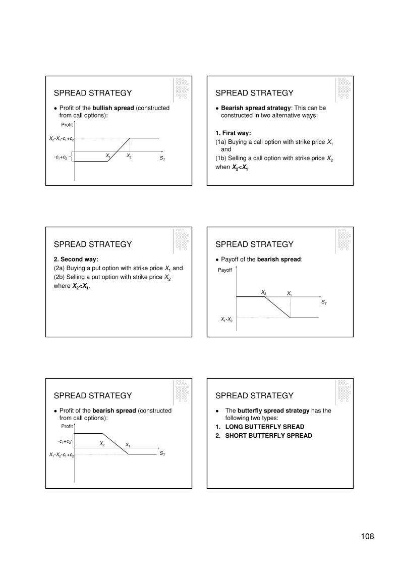
108
SPREAD STRATEGY
� Profit of the bullish spread (constructed from call options):
X1 X2
Profit
ST
X2-X1-c1+c2
-c1+c2
SPREAD STRATEGY
� Bearish spread strategy: This can be constructed in two alternative ways:
1. First way:
(1a) Buying a call option with strike price X1
and
(1b) Selling a call option with strike price X2
when X2<X1.
SPREAD STRATEGY
2. Second way:
(2a) Buying a put option with strike price X1 and
(2b) Selling a put option with strike price X2
where X2<X1.
SPREAD STRATEGY
� Payoff of the bearish spread:
ST
Payoff
X2 X1
X1-X2
SPREAD STRATEGY
� Profit of the bearish spread (constructed from call options):
ST
X2 X1
Profit
-c1+c2
X1-X2-c1+c2
SPREAD STRATEGY
� The butterfly spread strategy has the following two types:
1. LONG BUTTERFLY SREAD
2. SHORT BUTTERFLY SPREAD
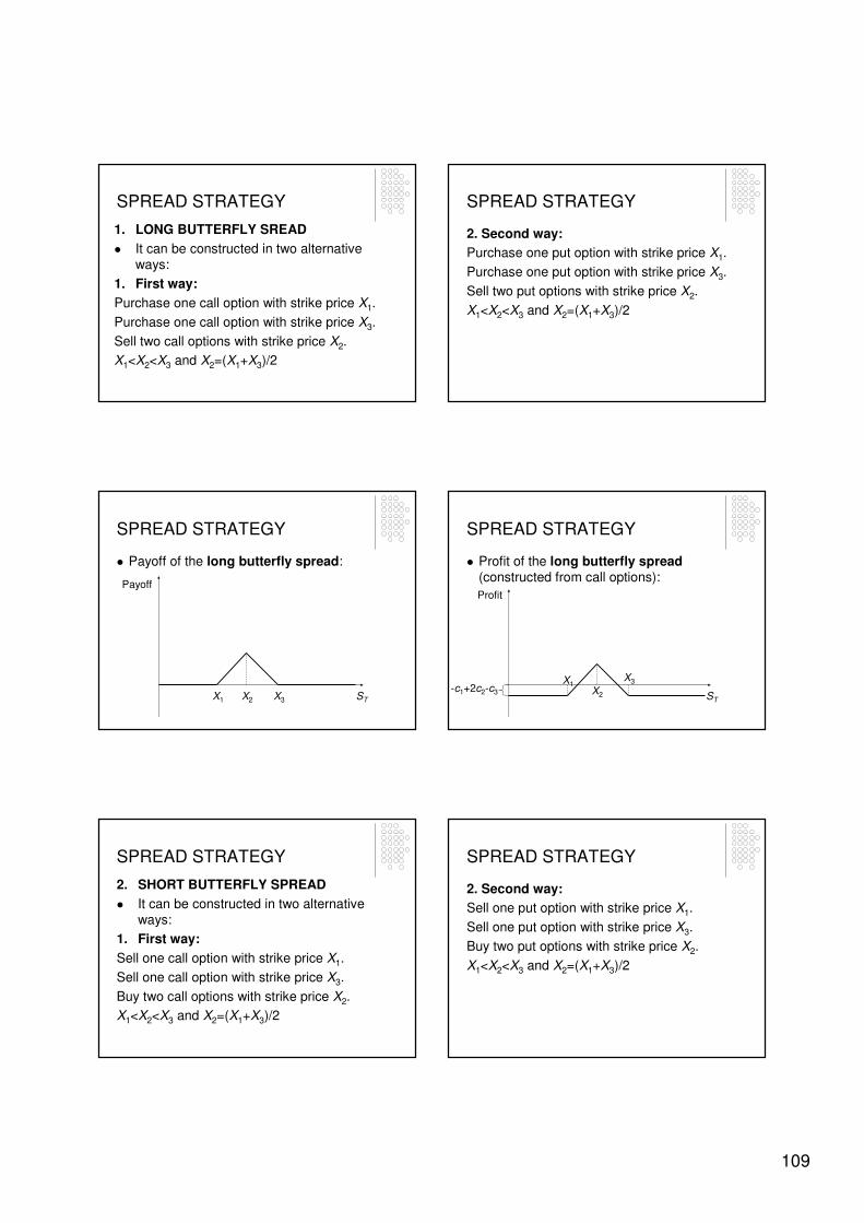
109
SPREAD STRATEGY
1. LONG BUTTERFLY SREAD
� It can be constructed in two alternative ways:
1. First way:
Purchase one call option with strike price X1.
Purchase one call option with strike price X3.
Sell two call options with strike price X2.
X1<X2<X3 and X2=(X1+X3)/2
SPREAD STRATEGY
2. Second way:
Purchase one put option with strike price X1.
Purchase one put option with strike price X3.
Sell two put options with strike price X2.
X1<X2<X3 and X2=(X1+X3)/2
SPREAD STRATEGY
� Payoff of the long butterfly spread:
X1 X2 X3 ST
Payoff
SPREAD STRATEGY
� Profit of the long butterfly spread (constructed from call options):
X1X2
X3
ST
Profit
-c1+2c2-c3
SPREAD STRATEGY
2. SHORT BUTTERFLY SPREAD
� It can be constructed in two alternative ways:
1. First way:
Sell one call option with strike price X1.
Sell one call option with strike price X3.
Buy two call options with strike price X2.
X1<X2<X3 and X2=(X1+X3)/2
SPREAD STRATEGY
2. Second way:
Sell one put option with strike price X1.
Sell one put option with strike price X3.
Buy two put options with strike price X2.
X1<X2<X3 and X2=(X1+X3)/2
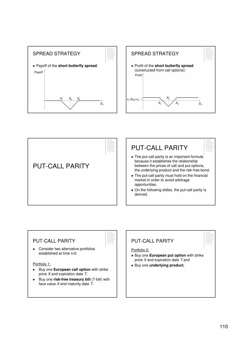
110
SPREAD STRATEGY
� Payoff of the short butterfly spread:
X1 X2 X3
ST
Payoff
SPREAD STRATEGY
� Profit of the short butterfly spread (constructed from call options):
X1
X2
X3 ST
Profit
c1-2c2+c3
PUT-CALL PARITY
PUT-CALL PARITY
� The put-call parity is an important formula because it establishes the relationship
between the prices of call and put options, the underlying product and the risk-free bond.
� The put-call parity must hold on the financial market in order to avoid arbitrage
opportunities.
� On the following slides, the put-call parity is derived.
PUT-CALL PARITY
� Consider two alternative portfolios established at time t=0:
Portfolio 1:
� Buy one European call option with strike price X and expiration date T.
� Buy one risk-free treasury bill (T-bill) with
face value X and maturity date T.
PUT-CALL PARITY
Portfolio 2:
� Buy one European put option with strike
price X and expiration date T and
� Buy one underlying product.
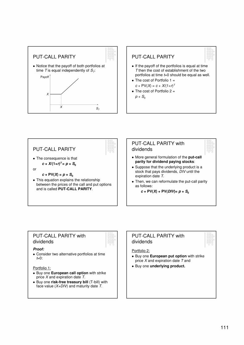
111
PUT-CALL PARITY
� Notice that the payoff of both portfolios at time T is equal independently of ST:
X
X
Payoff
ST
PUT-CALL PARITY
� If the payoff of the portfolios is equal at time T then the cost of establishment of the two
portfolios at time t=0 should be equal as well.
� The cost of Portfolio 1 =
c + PV(X) = c + X/(1+r)T
� The cost of Portfolio 2 =
p + S0
PUT-CALL PARITY
� The consequence is that
c + X/(1+r)T = p + S0
or
c + PV(X) = p + S0
� This equation explains the relationship
between the prices of the call and put options and is called PUT-CALL PARITY.
PUT-CALL PARITY withdividends
� More general formulation of the put-call parity for dividend paying stocks:
� Suppose that the underlying product is a
stock that pays dividends, DIV until the expiration date T.
� Then, we can reformulate the put-call parity as follows:
c + PV(X) + PV(DIV)= p + S0
PUT-CALL PARITY withdividends
Proof:
� Consider two alternative portfolios at time t=0:
Portfolio 1:
� Buy one European call option with strike price X and expiration date T.
� Buy one risk-free treasury bill (T-bill) with face value (X+DIV) and maturity date T.
PUT-CALL PARITY withdividends
Portfolio 2:
� Buy one European put option with strike
price X and expiration date T and
� Buy one underlying product.
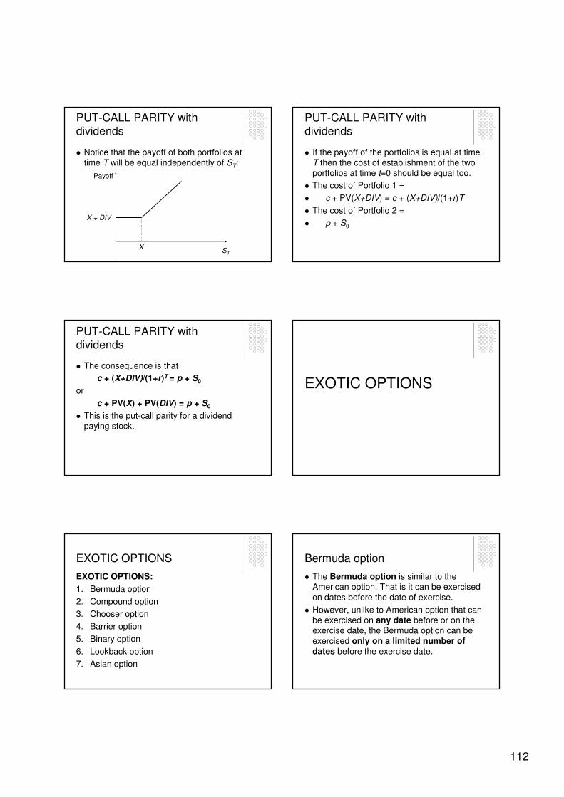
112
PUT-CALL PARITY with
dividends
� Notice that the payoff of both portfolios at time T will be equal independently of ST:
X
X + DIV
Payoff
ST
PUT-CALL PARITY with
dividends
� If the payoff of the portfolios is equal at time T then the cost of establishment of the two
portfolios at time t=0 should be equal too.
� The cost of Portfolio 1 =
� c + PV(X+DIV) = c + (X+DIV)/(1+r)T
� The cost of Portfolio 2 =
� p + S0
PUT-CALL PARITY withdividends
� The consequence is that
c + (X+DIV)/(1+r)T = p + S0
or
c + PV(X) + PV(DIV) = p + S0
� This is the put-call parity for a dividend
paying stock.
EXOTIC OPTIONS
EXOTIC OPTIONS
EXOTIC OPTIONS:
1. Bermuda option
2. Compound option
3. Chooser option
4. Barrier option
5. Binary option
6. Lookback option
7. Asian option
Bermuda option
� The Bermuda option is similar to the American option. That is it can be exercised
on dates before the date of exercise.
� However, unlike to American option that can be exercised on any date before or on the exercise date, the Bermuda option can be
exercised only on a limited number of dates before the exercise date.
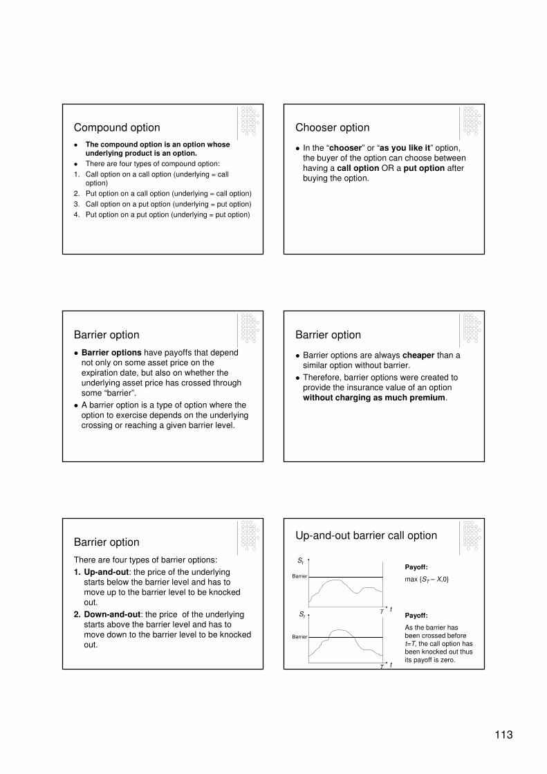
113
Compound option
� The compound option is an option whose underlying product is an option.
� There are four types of compound option:
1. Call option on a call option (underlying = call option)
2. Put option on a call option (underlying = call option)
3. Call option on a put option (underlying = put option)
4. Put option on a put option (underlying = put option)
Chooser option
� In the “chooser” or “as you like it” option, the buyer of the option can choose between
having a call option OR a put option after buying the option.
Barrier option
� Barrier options have payoffs that depend not only on some asset price on the
expiration date, but also on whether the underlying asset price has crossed through
some “barrier”.
� A barrier option is a type of option where the
option to exercise depends on the underlying crossing or reaching a given barrier level.
Barrier option
� Barrier options are always cheaper than a similar option without barrier.
� Therefore, barrier options were created to provide the insurance value of an option
without charging as much premium.
Barrier option
There are four types of barrier options:
1. Up-and-out: the price of the underlying starts below the barrier level and has to
move up to the barrier level to be knocked out.
2. Down-and-out: the price of the underlying starts above the barrier level and has to
move down to the barrier level to be knocked out.
Up-and-out barrier call option
St
t
tSt
Payoff:
max {ST – X,0}
Payoff:
As the barrier has been crossed before t=T, the call option has been knocked out thus
its payoff is zero.
Barrier
Barrier
T
T
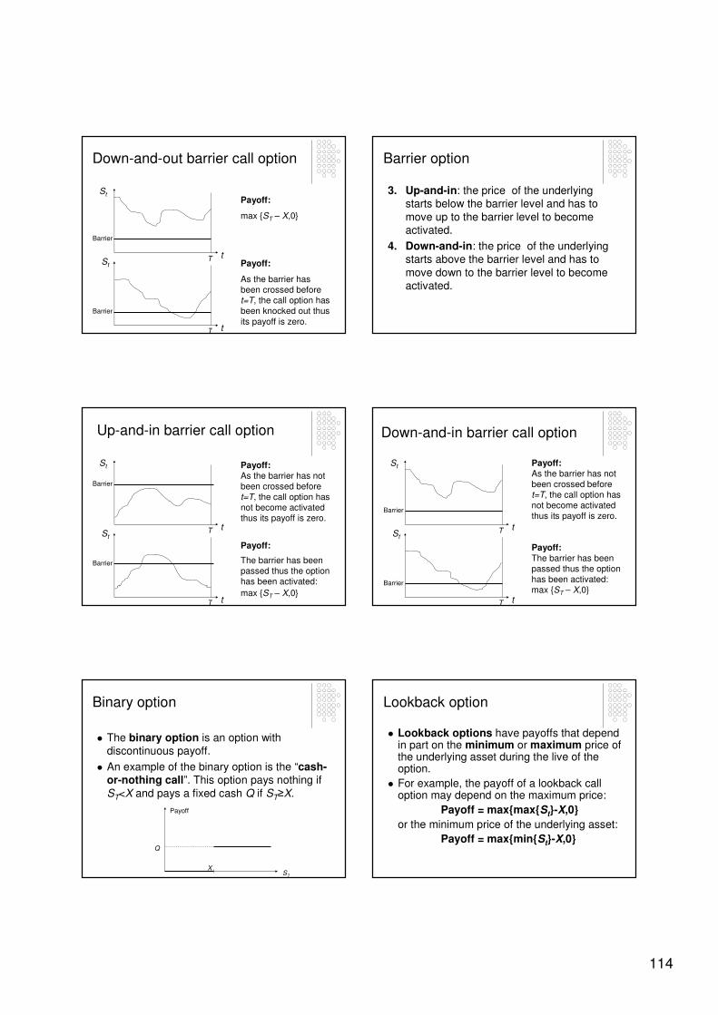
114
Down-and-out barrier call option
St
t
tSt
Payoff:
max {ST – X,0}
Payoff:
As the barrier has been crossed before t=T, the call option has been knocked out thus
its payoff is zero.
Barrier
Barrier
T
T
Barrier option
3. Up-and-in: the price of the underlying starts below the barrier level and has to
move up to the barrier level to become activated.
4. Down-and-in: the price of the underlying starts above the barrier level and has to
move down to the barrier level to become activated.
Up-and-in barrier call option
St
t
tSt
Payoff:As the barrier has not been crossed before t=T, the call option has not become activated thus its payoff is zero.
Payoff:
The barrier has been passed thus the option has been activated:
max {ST – X,0}
Barrier
Barrier
T
T
Down-and-in barrier call option
St
t
tSt
Payoff:As the barrier has not been crossed before t=T, the call option has not become activated thus its payoff is zero.
Payoff:The barrier has been passed thus the option has been activated:max {ST – X,0}
Barrier
Barrier
T
T
Binary option
� The binary option is an option with discontinuous payoff.
� An example of the binary option is the “cash-or-nothing call”. This option pays nothing if
ST<X and pays a fixed cash Q if ST≥X.
ST
X
Q
Payoff
Lookback option
� Lookback options have payoffs that depend in part on the minimum or maximum price of the underlying asset during the live of the option.
� For example, the payoff of a lookback call option may depend on the maximum price:
Payoff = max{max{St}-X,0}
or the minimum price of the underlying asset:
Payoff = max{min{St}-X,0}
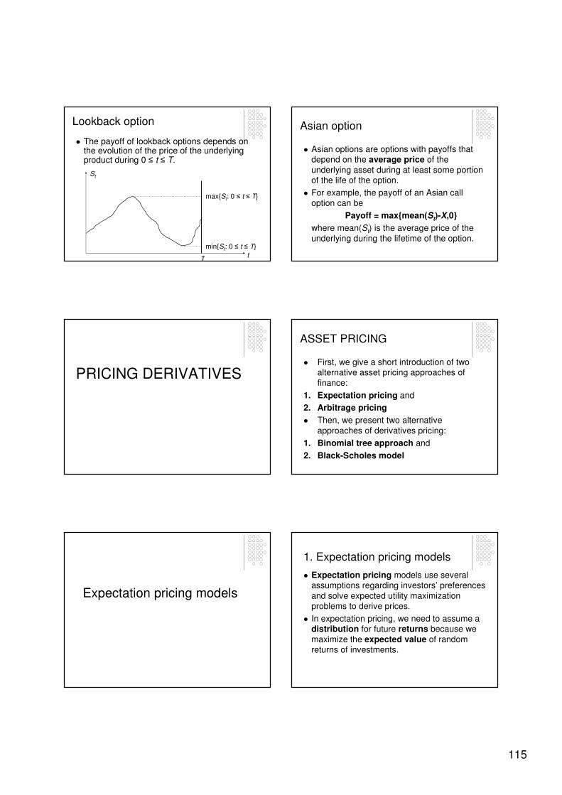
115
Lookback option
� The payoff of lookback options depends on the evolution of the price of the underlying product during 0 ≤ t ≤ T.
Tt
max{St: 0 ≤ t ≤ T}
min{St: 0 ≤ t ≤ T}
St
Asian option
� Asian options are options with payoffs that depend on the average price of the
underlying asset during at least some portion of the life of the option.
� For example, the payoff of an Asian call option can be
Payoff = max{mean(St)-X,0}
where mean(St) is the average price of the
underlying during the lifetime of the option.
PRICING DERIVATIVES
ASSET PRICING
� First, we give a short introduction of two alternative asset pricing approaches of
finance:
1. Expectation pricing and
2. Arbitrage pricing
� Then, we present two alternative
approaches of derivatives pricing:
1. Binomial tree approach and
2. Black-Scholes model
Expectation pricing models
1. Expectation pricing models
� Expectation pricing models use several assumptions regarding investors’ preferences
and solve expected utility maximization problems to derive prices.
� In expectation pricing, we need to assume a distribution for future returns because we
maximize the expected value of random returns of investments.
116
1. Expectation pricing models
� This assumption may fail easily and thus the prices obtained by expectation pricing are not
robust in general.
� Expectation pricing does not enforce market prices, it only gives a suggestion for market prices.
� A famous equilibrium pricing model is the
capital asset pricing model (CAPM).
Arbitrage pricing models
2. Arbitrage pricing models
� An alternative approach is arbitrage pricing, where we do not assume anything about the
‘real world’ probability distribution of future returns.
� Arbitrage pricing is more frequently used in practice then expectation pricing.
� Arbitrage pricing enforces market prices
therefore it is a more robust pricing result.
Arbitrage
� Definition (arbitrage opportunity): An arbitrage opportunity arises when the investor
can construct a zero investment portfolio that will yield a sure profit.
� In other words, the exploitation of security mispricing in such a way that risk-free
economic profits may be earned is called arbitrage.
Arbitrage
� It involves the simultaneous purchase and sale of equivalent securities in order to profit
from discrepancies in their price relationship, and so it is an extension of the law of one price.
� The concept of arbitrage is central to the
theory of financial markets.
Arbitrage
� Assumption: In order to be able to construct a zero investment portfolio, one has to be
able to sell short at least one asset and use the proceeds to purchase (to go long on) one
or more assets.
� Borrowing may be considered as a short
position in the risk-free asset.
� Even a small investor using short positions can take a large dollar / euro position in such
a portfolio.
117
Arbitrage
� A critical property of a risk-free arbitrage portfolio is that any investor, regardless of risk aversion or wealth, will want to take an infinite position in it so that profits will be driven to an infinite level.
� Because those large positions will force prices up or down until the opportunity vanishes, we can derive restrictions on security prices that satisfy the condition that no arbitrage opportunities are left in the marketplace.
Difference between arbitrage and expectation arguments
� Expectation pricing builds on investors’opinion about future returns, while arbitrage
pricing uses the price discrepancies among different assets.
� Therefore, we may say that expectation pricing leads to “absolute prices” and
arbitrage pricing derives “relative prices”.
Difference between arbitrage and
expectation arguments
� There is another important difference between arbitrage and expectation
arguments in support of equilibrium price relationships.
� When an expectation argument holds on the
market and the equilibrium price relationship is violated, many investors will make portfolio
changes.
Difference between arbitrage and expectation arguments
� In an expectation pricing model, each individual investor will make a limited change, though, depending on his or her degree of risk aversion.
� Aggregation of these limited portfolio changes over many investors is required to create a large volume of buying or selling, which in turn restores equilibrium prices.
Difference between arbitrage and expectation arguments
� However, when arbitrage opportunities exist, each investor wants to take as large position
as possible.
� Therefore, it will not take many investors to bring about price pressures necessary to restore equilibrium.
� For this reason, implications for prices
derived from no-arbitrage arguments are stronger than implications derived from a risk-
versus-return dominance argument.
DERIVATIVES PRICING
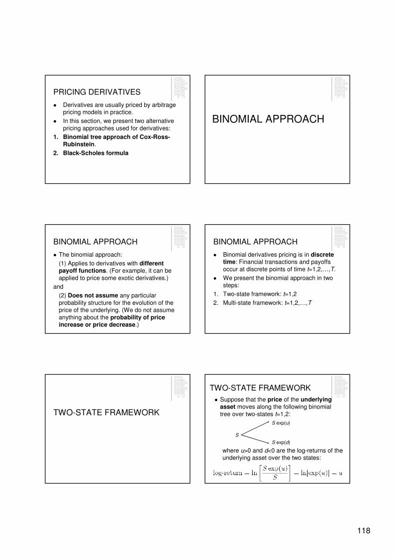
118
PRICING DERIVATIVES
� Derivatives are usually priced by arbitrage pricing models in practice.
� In this section, we present two alternative
pricing approaches used for derivatives:
1. Binomial tree approach of Cox-Ross-Rubinstein.
2. Black-Scholes formula
BINOMIAL APPROACH
BINOMIAL APPROACH
� The binomial approach:
(1) Applies to derivatives with different payoff functions. (For example, it can be
applied to price some exotic derivatives.)
and
(2) Does not assume any particular
probability structure for the evolution of the price of the underlying. (We do not assume
anything about the probability of price increase or price decrease.)
BINOMIAL APPROACH
� Binomial derivatives pricing is in discrete time: Financial transactions and payoffs
occur at discrete points of time t=1,2,…,T.
� We present the binomial approach in two steps:
1. Two-state framework: t=1,2
2. Multi-state framework: t=1,2,…,T
TWO-STATE FRAMEWORK
TWO-STATE FRAMEWORK
� Suppose that the price of the underlying asset moves along the following binomial
tree over two-states t=1,2:
S
S exp(d)
S exp(u)
where u>0 and d<0 are the log-returns of the underlying asset over the two states:

119
A REMARK ABOUT DISCOUNTING
� There are two alternative definitions of the discount factor that we use in this course:
(1) DF that uses “traditional returns”:
(2) DF that uses “log-returns”:
� In the derivatives pricing section, we use (2) to discount future cash flows.
TWO-STATE FRAMEWORK
� In the binomial tree approach, we do not need to assume anything about the
probability of price increase or price decrease.
� The only assumption we make about the evolution of S is that it goes along a binomial
tree. (That is in every period it goes up or down with certain log-return u or d.)
TWO-STATE FRAMEWORK
� We are interested in determining the price, fof a derivative whose payoff is a function of
the price of the underlying asset:
where f is the price of the derivative at t=1
and fu and fd are the payoffs of the derivative at t=2.
fu
fd
f
TWO-STATE FRAMEWORK
� In order to price the derivative, consider the following portfolio:
1. Buy ∆ units of the underlying asset
2. Sell 1 unit of the derivative
� If the price of the underlying goes up then the value of this portfolio at t=2 is
∆ S exp(u) – fuotherwise the value of this portfolio at t=2 is
∆ S exp(d) – fd
TWO-STATE FRAMEWORK
� First, we determine the value of ∆ that makes the portfolio risk-free.
� The portfolio is risk-free when its value is the
same either S goes up or down:
∆ S exp(u) – fu = ∆ S exp(d) – fd� From this equation, we get the number of
underlying assets that we need to buy to have a risk-free portfolio:
∆ = [fu-fd]/[S exp(u)–S exp(d)] (1)
TWO-STATE FRAMEWORK
� As the portfolio is risk-free, the price of the portfolio at t=1 is equal to the present value
of its payoff at t=2 computed using the risk-free rate, r:
∆ S – f = exp(-r) [∆ S exp(u) – fu]
� From this equation, we get the price of the derivative, f:
f = ∆ S - exp(-r) [∆ S exp(u) – fu] (2)

120
TWO-STATE FRAMEWORK
� We can get an alternative formula for the price of the derivative, f in the following
way:
� Substitute (1) into (2). Then, we get:
f = exp(-r) [p fu + (1-p) fd] (3)
where p is defined as
(4)
TWO-STATE FRAMEWORK
� Suppose that d ≤ r ≤ u. (This is a reasonable assumption because d is
negative, r is the risk-free rate and u is the rate of the risky underlying asset.)
� Then, it follows from equation (4) that 0 ≤p ≤ 1.
� Therefore, p can be interpreted as a
probability.
TWO-STATE FRAMEWORK
� If we interpret p in equation (4) as the probability that the price of S goes up then
equation (3) has a clear meaning:
� The price of the derivative is the present value, discounted by the risk-free rate, of the expected payoff of the derivative, where the expected value is computed using the probabilities p and (1-p).
TWO-STATE FRAMEWORK
� This pricing approach is very important in derivatives pricing.
� It is called risk-neutral pricing and the
probability p is called risk-neutral probability.
TWO-STATE FRAMEWORK
� Remark: Risk neutral pricing has nothing to do with expectation pricing because in risk
neutral pricing we use risk neutral probabilities to compute the expected payoff of the derivative whereas in expectation
pricing we use the real world probabilitiesfor the same computation.
TWO-STATE FRAMEWORK
� It is important to understand that the price of the derivative we have already obtained in
equation (2) before introducing the concept of the risk-neutral probability.
� Then, why did we introduce risk-neutral probability?
� Because equation (3) has a more clear and
intuitive meaning than (2): The price of the derivative is the present value of its expected payoff.
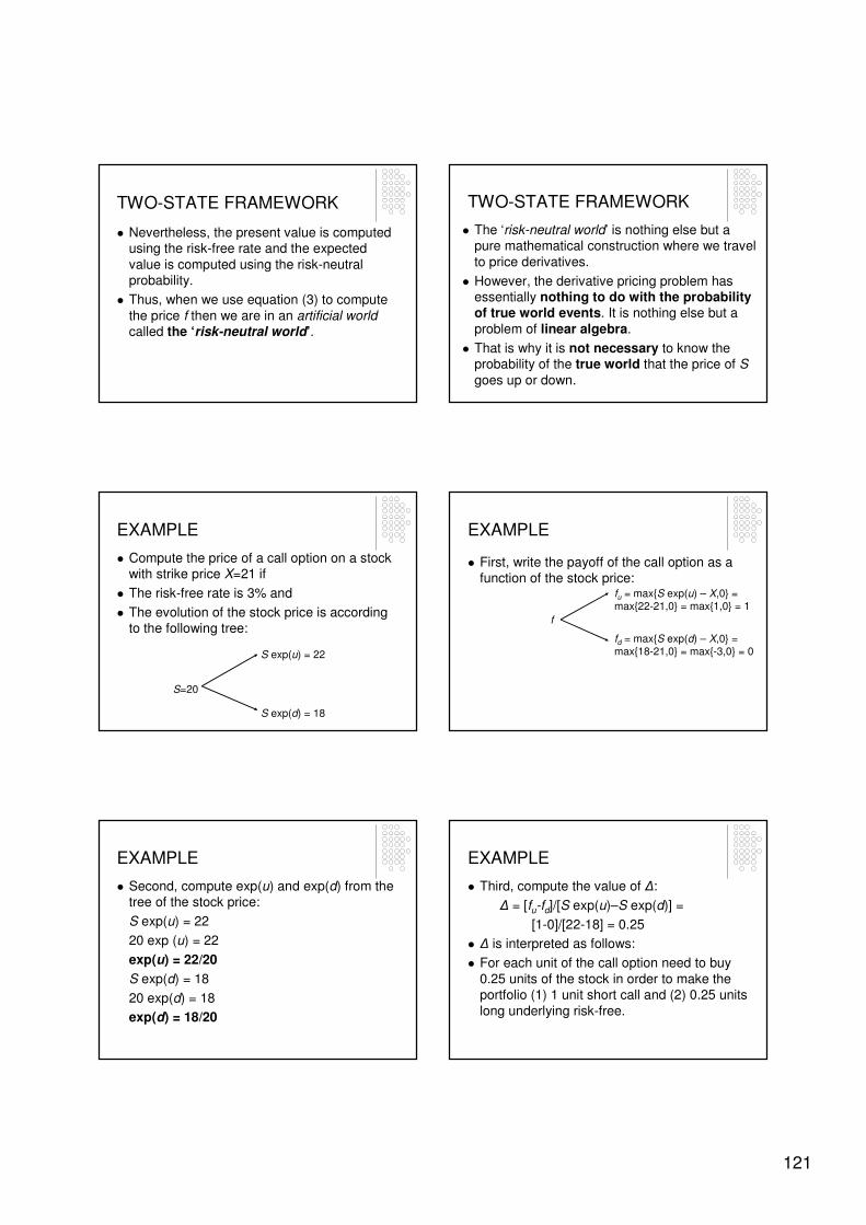
121
TWO-STATE FRAMEWORK
� Nevertheless, the present value is computed using the risk-free rate and the expected
value is computed using the risk-neutral probability.
� Thus, when we use equation (3) to compute
the price f then we are in an artificial worldcalled the ‘risk-neutral world’.
TWO-STATE FRAMEWORK
� The ‘risk-neutral world’ is nothing else but a pure mathematical construction where we travel
to price derivatives.
� However, the derivative pricing problem has essentially nothing to do with the probability of true world events. It is nothing else but a
problem of linear algebra.
� That is why it is not necessary to know the probability of the true world that the price of S
goes up or down.
EXAMPLE
� Compute the price of a call option on a stock with strike price X=21 if
� The risk-free rate is 3% and
� The evolution of the stock price is according to the following tree:
S=20
S exp(u) = 22
S exp(d) = 18
EXAMPLE
� First, write the payoff of the call option as a function of the stock price:
f
fu = max{S exp(u) – X,0} = max{22-21,0} = max{1,0} = 1
fd = max{S exp(d) – X,0} = max{18-21,0} = max{-3,0} = 0
EXAMPLE
� Second, compute exp(u) and exp(d) from the tree of the stock price:
S exp(u) = 22
20 exp (u) = 22
exp(u) = 22/20
S exp(d) = 18
20 exp(d) = 18
exp(d) = 18/20
EXAMPLE
� Third, compute the value of ∆:
∆ = [fu-fd]/[S exp(u)–S exp(d)] =
[1-0]/[22-18] = 0.25
� ∆ is interpreted as follows:
� For each unit of the call option need to buy
0.25 units of the stock in order to make the portfolio (1) 1 unit short call and (2) 0.25 units
long underlying risk-free.

122
EXAMPLE
� Next, we compute the value of the call option using formula (2):
f = ∆ S - exp(-r) [∆ S exp(u) – fu] =
0.25 x 20 – exp(3%) x [0.25 x 22 – 1] =
5 – 4.367 = 0.6330
� So the price of the call option is 0.6330.
EXAMPLE
� Alternatively, we can compute the price of the call option using the risk-neutral pricing of
equation (3):
f = exp(-r) [p fu + (1-p) fd]
� To do this this, first, we need to compute p:
p = [exp(r)-exp(d)]/[exp(u)-exp(d)] =
[exp(3%)-18/20]/[22/20-18/20] =
0.1304/0.2 = 0.652
EXAMPLE
� Now, we can compute equation (3):
f = exp(-r) [p fu + (1-p) fd] =
exp(-3%) x [0.652 x 1 + (1-0.652) x 0] =
0.6330
� So we get the same price for the call option as before: 0.6330.
MULTI-STATE FRAMEWORK
MULTI-STATE FRAMEWORK
� In the two-state methodology presented before we assumed that:
� There are only two-states t=1,2 and that
� There are only two possible outcomes of the price of the underlying asset (up or down).
� However, it would be more realistic if we
would have T-states t=1,2,…,T and more outcomes for the price of the underlying.
MULTI-STATE FRAMEWORK
� Therefore, we generalize the previous two-step framework to a multi-step setup.
� We may decide to model the price process
of the underlying asset according to the following two trees:
1. Recombining tree
2. Non-recombining tree

123
MULTI-STATE FRAMEWORKRECOMBINING TREE
Notice that on this figure t=1,…,4 and the
number of possible outcomes is 4.
MULTI-STATE FRAMEWORKNON-RECOMBINING TREE
Notice that on this figure t=1,…,4 and the
number of possible outcomes is 8.
MULTI-STATE FRAMEWORK
� We can see that the non-recombining tree allows more outcomes, i.e. it is more general.
� The pricing approach to be discussed applies
to both types of trees.
� However, it is computationally easier to work
with the recombining tree.
� In the followings, we focus on the recombining tree to compute prices.
MULTI-STATE FRAMEWORK
Notice that the multi-state tree is simply the
sum of two-state trees.
MULTI-STATE FRAMEWORK
� If we think of the multi-state tree as the sum of several two-state trees then we can easily
apply the approach introduced in the two-state slides for the multi-state tree.
� To show how to do it in practice we consider three states:
MULTI-STATE FRAMEWORK
� This is the tree of prices of the underlying
asset.
S exp(2u)
S exp(u+d)
S exp(2d)
S exp(u)
S exp(d)
S
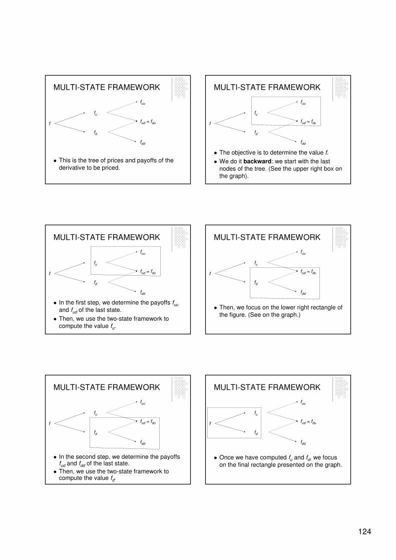
124
MULTI-STATE FRAMEWORK
� This is the tree of prices and payoffs of the
derivative to be priced.
fuu
fud = fdu
fdd
fu
fd
f
MULTI-STATE FRAMEWORK
� The objective is to determine the value f.
� We do it backward: we start with the last
nodes of the tree. (See the upper right box on the graph).
fuu
fud = fdu
fdd
fu
fd
f
MULTI-STATE FRAMEWORK
� In the first step, we determine the payoffs fuu
and fud of the last state.
� Then, we use the two-state framework to compute the value fu.
fuu
fud = fdu
fdd
fu
fd
f
MULTI-STATE FRAMEWORK
� Then, we focus on the lower right rectangle of
the figure. (See on the graph.)
fuu
fud = fdu
fdd
fu
fd
f
MULTI-STATE FRAMEWORK
� In the second step, we determine the payoffs fud and fdd of the last state.
� Then, we use the two-state framework to compute the value fd.
fuu
fud = fdu
fdd
fu
fd
f
MULTI-STATE FRAMEWORK
� Once we have computed fu and fd, we focus
on the final rectangle presented on the graph.
fuu
fud = fdu
fdd
fu
fd
f
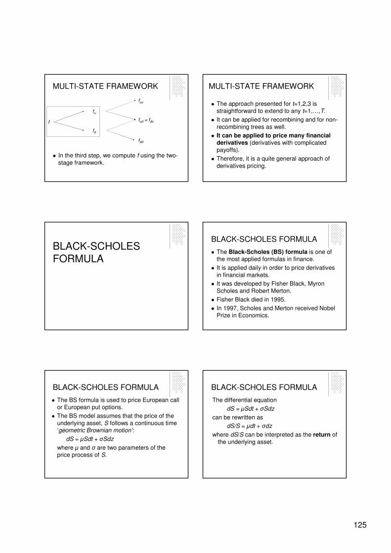
125
MULTI-STATE FRAMEWORK
� In the third step, we compute f using the two-
stage framework.
fuu
fud = fdu
fdd
fu
fd
f
� The approach presented for t=1,2,3 is straightforward to extend to any t=1,…,T.
� It can be applied for recombining and for non-
recombining trees as well.
� It can be applied to price many financial derivatives (derivatives with complicated payoffs).
� Therefore, it is a quite general approach of
derivatives pricing.
MULTI-STATE FRAMEWORK
BLACK-SCHOLES
FORMULA
BLACK-SCHOLES FORMULA
� The Black-Scholes (BS) formula is one of the most applied formulas in finance.
� It is applied daily in order to price derivatives
in financial markets.
� It was developed by Fisher Black, Myron
Scholes and Robert Merton.
� Fisher Black died in 1995.
� In 1997, Scholes and Merton received Nobel Prize in Economics.
BLACK-SCHOLES FORMULA
� The BS formula is used to price European call or European put options.
� The BS model assumes that the price of the
underlying asset, S follows a continuous time ‘geometric Brownian motion’:
dS = µSdt + σSdz
where µ and σ are two parameters of the price process of S.
BLACK-SCHOLES FORMULA
The differential equation
dS = µSdt + σSdz
can be rewritten as
dS/S = µdt + σdz
where dS/S can be interpreted as the return of
the underlying asset.
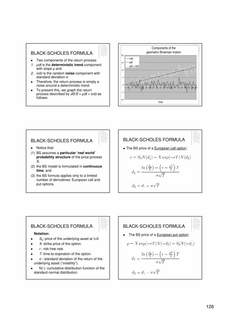
126
BLACK-SCHOLES FORMULA
� Two components of the return process:
1. µdt is the deterministic trend component with slope µ and
2. σdz is the random noise component with standard deviation σ.
� Therefore, the return process is simply a noise around a deterministic trend.
� To present this, we graph the return process described by dS/S = µdt + σdz as follows:
Components of the
geometric Brownian motion
-10
-5
0
5
10
15
20
1 6 11 16 21 26 31 36 41 46 51 56 61 66 71 76 81 86 91 96 101
time
σdz
µdt
µdt + σdz
BLACK-SCHOLES FORMULA
� Notice that:
(1) BS assumes a particular ‘real world’probability structure of the price process
S,
(2) the BS model is formulated in continuous time, and
(3) the BS formula applies only to a limited number of derivatives: European call and
put options.
BLACK-SCHOLES FORMULA
� The BS price of a European call option:
BLACK-SCHOLES FORMULA
Notation:
� S0: price of the underlying asset at t=0.
� X: strike price of the option.
� r : risk-free rate.
� T: time-to-expiration of the option.
� σ : standard deviation of the return of the
underlying asset (“volatility”).
� N(·): cumulative distribution function of the
standard normal distribution.
BLACK-SCHOLES FORMULA
� The BS price of a European put option:
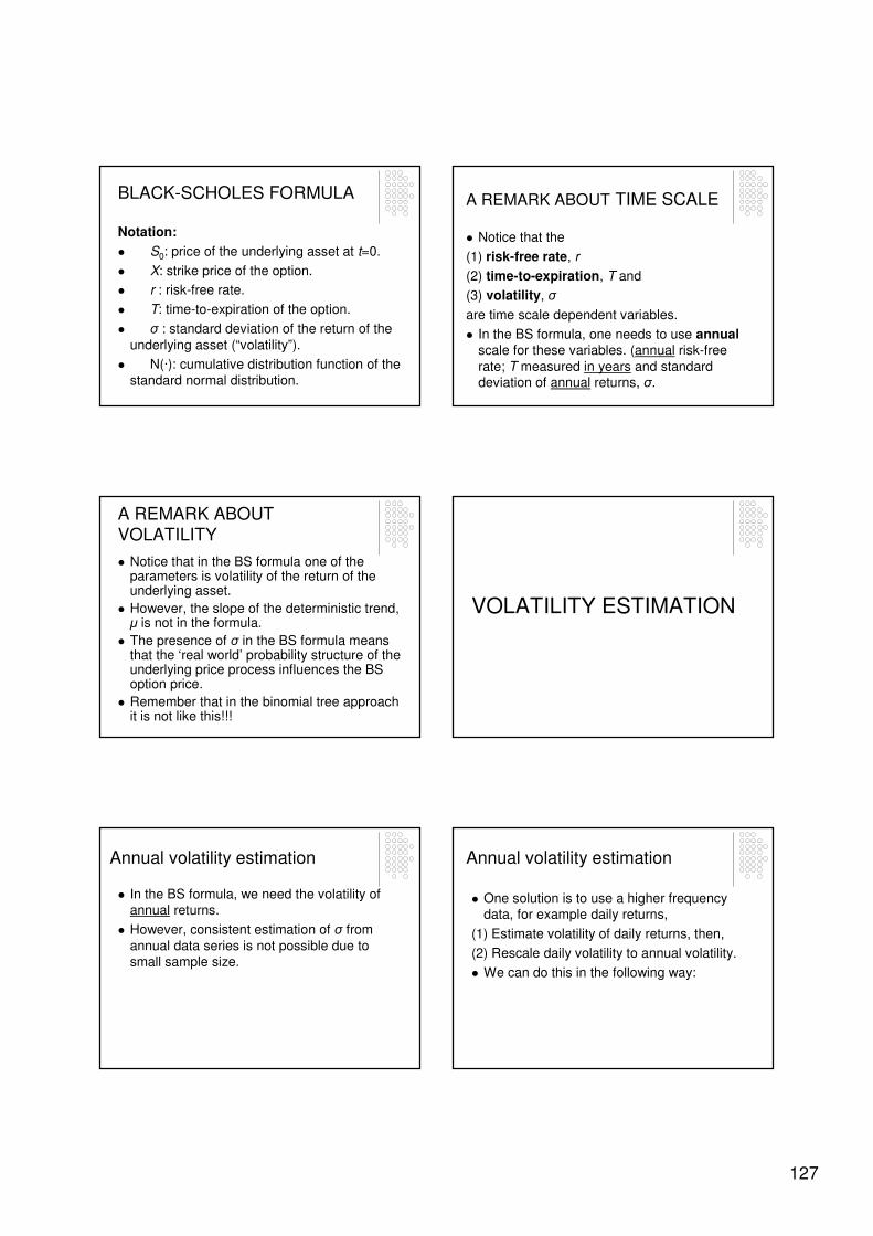
127
BLACK-SCHOLES FORMULA
Notation:
� S0: price of the underlying asset at t=0.
� X: strike price of the option.
� r : risk-free rate.
� T: time-to-expiration of the option.
� σ : standard deviation of the return of the
underlying asset (“volatility”).
� N(·): cumulative distribution function of the
standard normal distribution.
A REMARK ABOUT TIME SCALE
� Notice that the
(1) risk-free rate, r
(2) time-to-expiration, T and
(3) volatility, σ
are time scale dependent variables.
� In the BS formula, one needs to use annualscale for these variables. (annual risk-free
rate; T measured in years and standard deviation of annual returns, σ.
A REMARK ABOUT VOLATILITY
� Notice that in the BS formula one of the parameters is volatility of the return of the underlying asset.
� However, the slope of the deterministic trend, µ is not in the formula.
� The presence of σ in the BS formula means that the ‘real world’ probability structure of the underlying price process influences the BS option price.
� Remember that in the binomial tree approach it is not like this!!!
VOLATILITY ESTIMATION
Annual volatility estimation
� In the BS formula, we need the volatility of annual returns.
� However, consistent estimation of σ from
annual data series is not possible due to small sample size.
Annual volatility estimation
� One solution is to use a higher frequency data, for example daily returns,
(1) Estimate volatility of daily returns, then,
(2) Rescale daily volatility to annual volatility.
� We can do this in the following way:
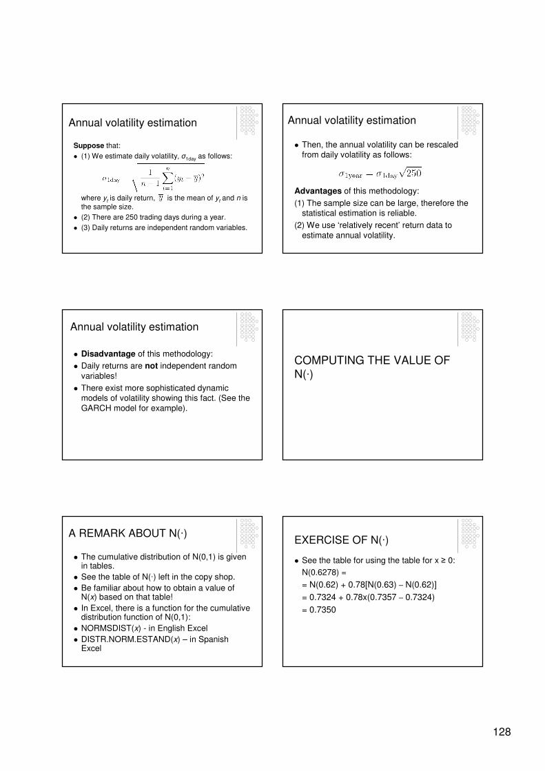
128
Annual volatility estimation
Suppose that:
� (1) We estimate daily volatility, σ1day as follows:
where yt is daily return, is the mean of yt and n is
the sample size.
� (2) There are 250 trading days during a year.
� (3) Daily returns are independent random variables.
Annual volatility estimation
� Then, the annual volatility can be rescaled from daily volatility as follows:
Advantages of this methodology:
(1) The sample size can be large, therefore the statistical estimation is reliable.
(2) We use ‘relatively recent’ return data to
estimate annual volatility.
Annual volatility estimation
� Disadvantage of this methodology:
� Daily returns are not independent random
variables!
� There exist more sophisticated dynamic models of volatility showing this fact. (See the
GARCH model for example).
COMPUTING THE VALUE OF
N(·)
A REMARK ABOUT N(·)
� The cumulative distribution of N(0,1) is given in tables.
� See the table of N(·) left in the copy shop.
� Be familiar about how to obtain a value of N(x) based on that table!
� In Excel, there is a function for the cumulative distribution function of N(0,1):
� NORMSDIST(x) - in English Excel
� DISTR.NORM.ESTAND(x) – in Spanish Excel
EXERCISE OF N(·)
� See the table for using the table for x ≥ 0:
N(0.6278) =
= N(0.62) + 0.78[N(0.63) – N(0.62)]
= 0.7324 + 0.78x(0.7357 – 0.7324)
= 0.7350
129
EXERCISE OF N(·)
� See the table for using the table for x ≤ 0:
N(-0.1234)=
= N(-0.12) – 0.34[N(-0.12) – N(-0.13)]
= 0.4522 – 0.34x(0.4522 – 0.4483)
= 0.4509
EXERCISE OF N(·)
� Use the table of the N(0,1) distribution to compute N(x) for the next values of x:
(a) x = 0.0521
(b) x = 0.1367
(c) x = 2.4701
(d) x = -0.0012
(e) x = -1.5419
(f) x = -2.3177
(a) x = 0.0521
� N(0.0521) =
N(0.05) + 0.21[N(0.06) - N(0.05)] =
0.5199 + 0.21[0.5239 – 0.5199] =
0.5207
(b) x = 0.1367
� N(0.1367) =
N(0.13) + 0.67[N(0.14) – N(0.13)] =
0.5517 + 0.67[0.5557 – 0.5517] =
0.5544
(c) x = 2.4701
� N(2.4701)=
N(2.47) + 0.01[N(2.48)-N(2.47)] =
0.9932 + 0.01[0.9934 – 0.9932] =
0.9932
(d) x = -0.0012
� N(-0.0012)=
N(-0.00) – 0.12[N(-0.00) – N(-0.01)] =
0.5 – 0.12[0.5 – 0.4960] =
0.4995
130
(e) x = -1.5419
� N(-1.5419) =
N(-1.54) - 0.19[N(-1.54) – N(-1.55)] =
0.0618 – 0.19[0.0618 – 0.0606] =
0.0616
(f) x = -2.3177
� N(-2.3177) =
N(-2.31) – 0.77[N(-2.31) – N(-2.32)] =
0.0104 – 0.77[0.0104 – 0.0102] =
0.0102
RISK MANAGEMENT OF
OPTIONS CONTRACTS
RISK MANAGEMENT OF OPTIONS
� In the previous section, we priced options in a static setup:
� We computed the price of derivatives at time
t = 0.
� However, in the reality we are in a dynamic
setup: t = 0,...,T.
� This means that investors are interested in the evolution of the prices in their portfolios
over time.
RISK MANAGEMENT OF OPTIONS
� In this section, we are going to analyze to risks associated to European optioncontracts in the BS framework.
� Remember from the BS formulas that the
price of an option is determined by the next five elements:
RISK MANAGEMENT OF OPTIONS
1. Strike price, X
2. Time to expiration, T
3. Risk-free interest rate, r
4. Spot price of the underlying asset, S0
5. Volatility of the underlying asset return, σ

131
RISK MANAGEMENT OF OPTIONS
� Notice that in a dynamic setup X and T are fixed in the option contract at time t = 0. Thus, they do not change over time.
� However, also notice that r, S0 and σ change over time. These are the risk factors of option prices.
� (Remark: The S0 notation may be misleading. It denotes that actual price of the underlying asset. Thus, as time is passing in a dynamic setup, the price of the underlying asset also changes.)
RISK MANAGEMENT OF OPTIONS
� In the remaining part of this section, for simplicity, we are going to assume that r and
σ are constant over time.
� We will focus only on the impact of changing S0 on the option price.
RISK MANAGEMENT OF OPTIONS
� For a portfolio manager, it is important to know the sensitivity of option prices to the
price of the underlying asset in order to
� (1) measure the risk of option and
� (2) construct risk-free portfolios of options
and underlying assets.
SENSITIVITY OF OPTION PRICE
� We have seen in the BS formulas that the price of an option depends on the price of the
underlying asset, S0.
� The sensitivity of c and p to S0 can be approximated by the partial derivatives of the c(S0) and p(S0) functions with respect to
S0.
SENSITIVITY OF OPTION PRICE
� Notice that the option price in the BS formulas in a non-linear function of S0.
� Therefore, if one considers only the first
derivative of c(S0) and p(S0) to measure the sensitivity of the option price (i.e., we do a linear approximation), we shall not be
precise.
� This fact is presented on the following figure:
APPROXIMATION OF PRICE CHANGE FOR A CALL OPTION
S0
c
S’S
Total change of c = (3) = (1) + (2) =
delta approximation + error
(3)
(1)
(2)
c(S)
c(S’)
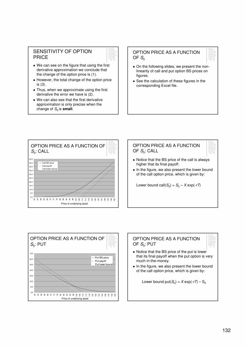
132
SENSITIVITY OF OPTION PRICE
� We can see on the figure that using the first derivative approximation we conclude that
the change of the option price is (1).
� However, the total change of the option price is (3).
� Thus, when we approximate using the first derivative the error we have is (2).
� We can also see that the first derivative
approximation is only precise when the change of S0 is small.
OPTION PRICE AS A FUNCTION OF S0
� On the following slides, we present the non-linearity of call and put option BS prices on
figures.
� See the calculation of these figures in the
corresponding Excel file.
0.0
5.0
10.0
15.0
20.0
25.0
30.0
35.0
40.0
45.0
50.0
50
54
58
62
66
70
74
78
82
86
90
94
98
102
106
110
114
118
122
126
130
134
138
142
146
150
Price of underlying asset
Call BS price
Call payoff
Call lower bound
OPTION PRICE AS A FUNCTION OF
S0: CALL
OPTION PRICE AS A FUNCTION OF S0: CALL
� Notice that the BS price of the call is always higher that its final payoff.
� In the figure, we also present the lower bound of the call option price, which is given by:
Lower bound call(S0) = S0 – X exp(-rT)
0.0
10.0
20.0
30.0
40.0
50.0
60.0
70.0
50
54
58
62
66
70
74
78
82
86
90
94
98
102
106
110
114
118
122
126
130
134
138
142
146
150
Price of underlying asset
Put BS price
Put payoff
Put lower bound
OPTION PRICE AS A FUNCTION OF
S0: PUT
OPTION PRICE AS A FUNCTION OF S0: PUT
� Notice that the BS price of the put is lower that its final payoff when the put option is very
much in-the-money.
� In the figure, we also present the lower bound of the call option price, which is given by:
Lower bound put(S0) = X exp(-rT) – S0
133
SENSITIVITY OF OPTION PRICE
� In the followings, we shall proceed in two steps:
� First, we shall use the first derivative to
measure option price sensitivity.
DELTA of the option
� Second, we will employ both the first and
second derivatives to approximate the sensitivity of option prices.
DELTA and GAMMA of the option
1. DELTA OF THE OPTION:
DELTA HEDGE
1. DELTA
� The first derivative of the option price with
respect to the price of the underlying asset is called delta and is denoted by ∆.
1. DELTA
� The delta of the call and put options can be approximated as follows in the BS model:
∆c = ∂c/∂S0 ≈ N(d1) > 0
∆p = ∂p/∂S0 ≈ -N(-d1) = N(d1)-1 < 0
where d1 is computed as before:
and N(·) is the cumulative distribution function of N(0,1).
1. DELTA
� Notice that on the previous slide we only show an approximate result for the deltas.
� This is because to exact derivative of the
c(S0) and p(S0) functions are not the reported ones.
� In fact, reviewing the BS formulas, we see that both d1 and d2 also depend on S0, which
should be differentiated too to get the exact formula.
1. DELTA
� However, the presented approximations of delta are precise enough to be used in
practice.
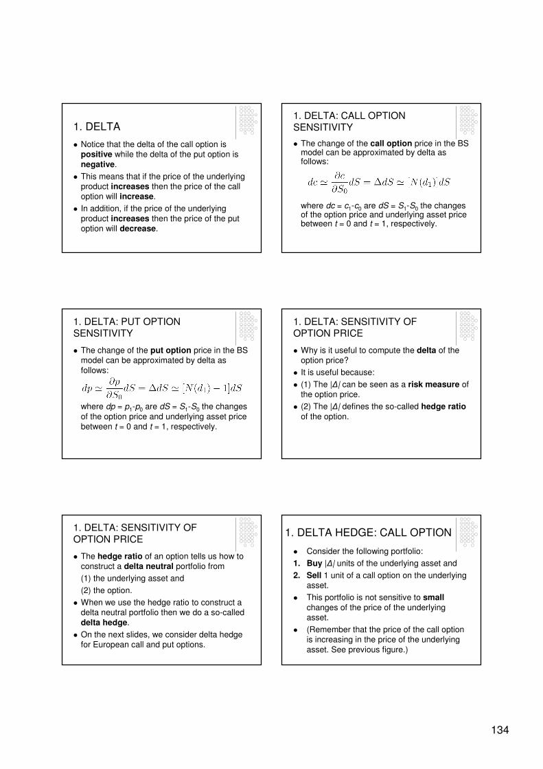
134
1. DELTA
� Notice that the delta of the call option is positive while the delta of the put option is
negative.
� This means that if the price of the underlying product increases then the price of the call option will increase.
� In addition, if the price of the underlying
product increases then the price of the put option will decrease.
1. DELTA: CALL OPTION SENSITIVITY
� The change of the call option price in the BS model can be approximated by delta as follows:
where dc = c1-c0 are dS = S1-S0 the changes of the option price and underlying asset price between t = 0 and t = 1, respectively.
1. DELTA: PUT OPTION SENSITIVITY
� The change of the put option price in the BS model can be approximated by delta as
follows:
where dp = p1-p0 are dS = S1-S0 the changes
of the option price and underlying asset price between t = 0 and t = 1, respectively.
1. DELTA: SENSITIVITY OF OPTION PRICE
� Why is it useful to compute the delta of the option price?
� It is useful because:
� (1) The |∆| can be seen as a risk measure of the option price.
� (2) The |∆| defines the so-called hedge ratioof the option.
1. DELTA: SENSITIVITY OF OPTION PRICE
� The hedge ratio of an option tells us how to construct a delta neutral portfolio from
(1) the underlying asset and
(2) the option.
� When we use the hedge ratio to construct a delta neutral portfolio then we do a so-called
delta hedge.
� On the next slides, we consider delta hedge for European call and put options.
1. DELTA HEDGE: CALL OPTION
� Consider the following portfolio:
1. Buy |∆| units of the underlying asset and
2. Sell 1 unit of a call option on the underlying asset.
� This portfolio is not sensitive to smallchanges of the price of the underlying asset.
� (Remember that the price of the call option is increasing in the price of the underlying
asset. See previous figure.)

135
1. DELTA HEDGE: PUT OPTION
� Consider the following portfolio:
1. Buy |∆| units of the underlying asset and
2. Buy 1 unit of a put option on the underlying asset.
� This portfolio is not sensitive to smallchanges of the price of the underlying asset.
� (Remember that the price of the put option
is decreasing in the price of the underlying asset. See previous figure.)
1. THE DELTA HEDGE RATIO FORMULA
Disadvantage:
� One can hedge only small changes of the underlying asset price.
Advantage:
� The formula includes terms known at time t = 0.
� In other words, the risk manager can compute
this hedge ratio using information observed at time t = 0.
1. DELTA HEDGE
� We shall see an example later for the computation of delta and delta hedge.
2. GAMMA OF THE OPTION:
DELTA-GAMMA HEDGE
2. GAMMA: MOTIVATION
� As we have seen before, the price of an option is non-linear function of S0 in the BS
formulas.
� This means that the first derivative is only a linear approximation of the total change of option price for the change of S0 and works
only if the change of S0 is small.
2. GAMMA: MOTIVATION
� A more reliable, non-linear approximation of the sensitivity of option price to S0 is obtained when we take into account the second partial derivative of the option price as well.
� First, we will present how to compute to second derivative, called gamma, of an option in the BS framework.
� Then, we shall approximate the sensitivity of option price using both delta and gamma.
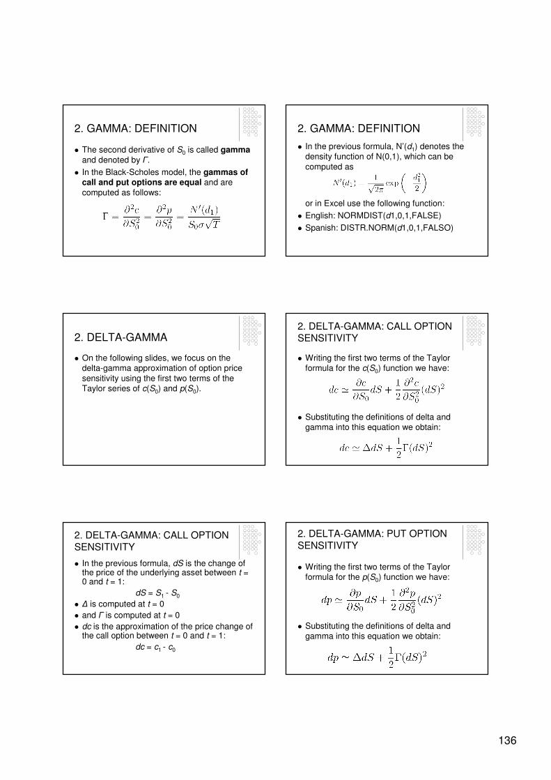
136
2. GAMMA: DEFINITION
� The second derivative of S0 is called gammaand denoted by Γ.
� In the Black-Scholes model, the gammas of call and put options are equal and are
computed as follows:
2. GAMMA: DEFINITION
� In the previous formula, N’(d1) denotes the density function of N(0,1), which can be
computed as
or in Excel use the following function:
� English: NORMDIST(d1,0,1,FALSE)
� Spanish: DISTR.NORM(d1,0,1,FALSO)
2. DELTA-GAMMA
� On the following slides, we focus on the delta-gamma approximation of option price
sensitivity using the first two terms of the Taylor series of c(S0) and p(S0).
2. DELTA-GAMMA: CALL OPTION SENSITIVITY
� Writing the first two terms of the Taylor formula for the c(S0) function we have:
� Substituting the definitions of delta and gamma into this equation we obtain:
2. DELTA-GAMMA: CALL OPTION SENSITIVITY
� In the previous formula, dS is the change of the price of the underlying asset between t = 0 and t = 1:
dS = S1 - S0
� ∆ is computed at t = 0
� and Γ is computed at t = 0
� dc is the approximation of the price change of the call option between t = 0 and t = 1:
dc = c1 - c0
2. DELTA-GAMMA: PUT OPTION
SENSITIVITY
� Writing the first two terms of the Taylor formula for the p(S0) function we have:
� Substituting the definitions of delta and gamma into this equation we obtain:
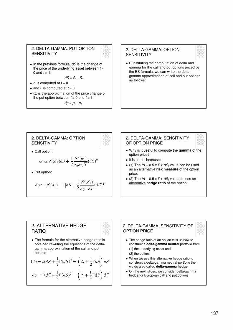
137
2. DELTA-GAMMA: PUT OPTION
SENSITIVITY
� In the previous formula, dS is the change of the price of the underlying asset between t = 0 and t = 1:
dS = S1 - S0
� ∆ is computed at t = 0
� and Γ is computed at t = 0
� dp is the approximation of the price change of the put option between t = 0 and t = 1:
dp = p1 - p0
2. DELTA-GAMMA: OPTION SENSITIVITY
� Substituting the computation of delta and gamma for the call and put options priced by
the BS formula, we can write the delta-gamma approximation of call and put options as follows:
2. DELTA-GAMMA: OPTION SENSITIVITY
� Call option:
� Put option:
2. DELTA-GAMMA: SENSITIVITY OF OPTION PRICE
� Why is it useful to compute the gamma of the option price?
� It is useful because:
� (1) The |∆ + 0.5 x Γ x dS| value can be used as an alternative risk measure of the option
price.
� (2) The |∆ + 0.5 x Γ x dS| value defines an alternative hedge ratio of the option.
2. ALTERNATIVE HEDGE RATIO
� The formula for the alternative hedge ratio is obtained rewriting the equations of the delta-
gamma approximation of the call and put options:
2. DELTA-GAMMA: SENSITIVITY OF
OPTION PRICE
� The hedge ratio of an option tells us how to
construct a delta-gamma neutral portfolio from
(1) the underlying asset and
(2) the option.
� When we use this alternative hedge ratio to
construct a delta-gamma neutral portfolio then we do a so-called delta-gamma hedge.
� On the next slides, we consider delta-gamma hedge for European call and put options.

138
2. DELTA-GAMMA HEDGE: CALL
OPTION� Consider the following portfolio:
1. Buy |∆ + 0.5 x Γ x dS| units of the underlying asset and
2. Sell 1 unit of a call option on the underlying asset.
� This portfolio is not sensitive to largechanges of the price of the underlying asset.
� (Remember that the price of the call option is increasing in the price of the underlying asset.)
2. DELTA-GAMMA HEDGE: PUT
OPTION
� Consider the following portfolio:
1. Buy |∆ + 0.5 x Γ x dS| units of the underlying asset and
2. Buy 1 unit of a put option on the underlying asset.
� This portfolio is not sensitive to largechanges of the price of the underlying asset.
� (Remember that the price of the put option is decreasing in the price of the underlying asset.)
2. THE DELTA-GAMMA HEDGE
RATIO FORMULA
Advantage:
� One can hedge large changes of the
underlying asset price.
Disadvantage:
� The formula includes the dS=S1-S0 term and
S1 is not known at time t = 0.
� Thus, the risk manager needs to suppose a future price for the underlying asset.
OPTION RISK MANAGEMENT: TWO EXAMPLES
� You are a financial risk manager of BBVA.
� You have to
(Ex.1) Compute the delta and gamma of a European call and a European put option and approximate the future change of the
option prices using these values.
(Ex.2) Form a delta neutral and a delta-gamma neutral portfolio from the options and their
underlying asset.
OPTION RISK MANAGEMENT: TWO EXAMPLES
� On the next slides, we solve these two tasks in examples 1 and 2.
EXAMPLE 1:
DELTA-GAMMA APPROXIMATION
(1) Compute the delta and gamma of a European call and a European put option
and approximate the future change of the option prices using these values.
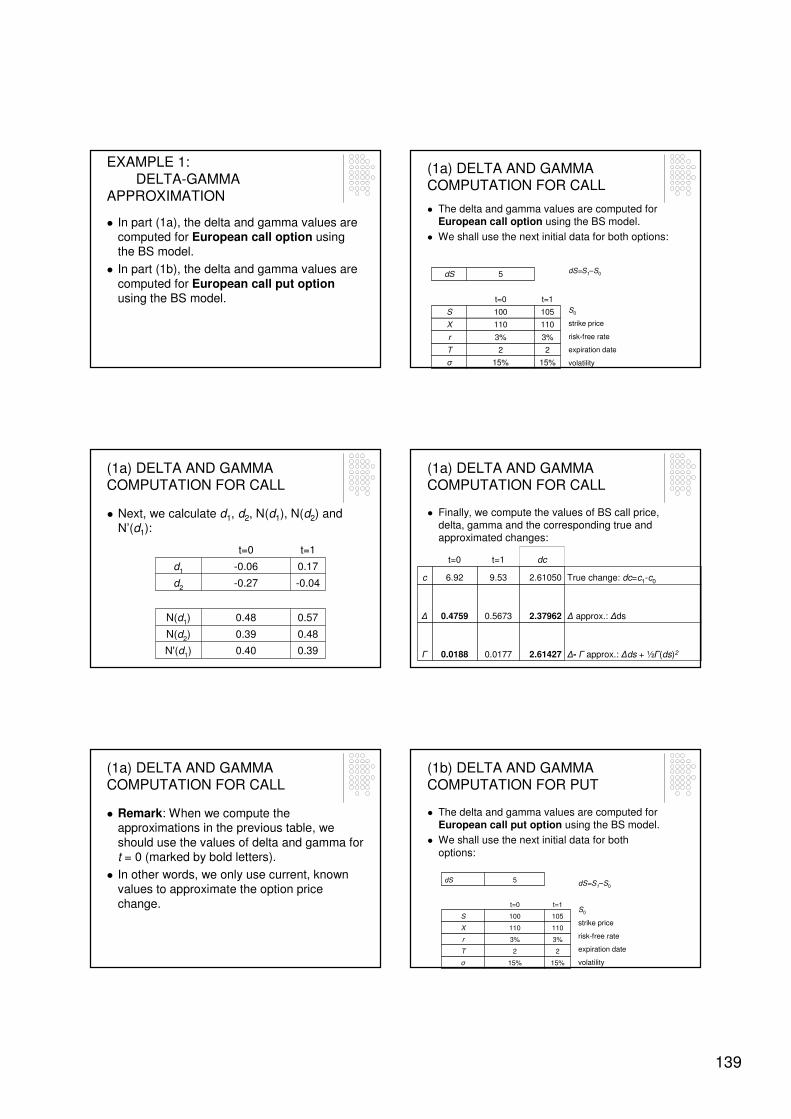
139
EXAMPLE 1:
DELTA-GAMMA APPROXIMATION
� In part (1a), the delta and gamma values are computed for European call option using the BS model.
� In part (1b), the delta and gamma values are
computed for European call put optionusing the BS model.
(1a) DELTA AND GAMMA COMPUTATION FOR CALL
� The delta and gamma values are computed for European call option using the BS model.
� We shall use the next initial data for both options:
15%15%σ
22T
3%3%r
110110X
105100S
t=1t=0
5dS dS=S1–S0
S0
strike price
risk-free rate
expiration date
volatility
(1a) DELTA AND GAMMA COMPUTATION FOR CALL
� Next, we calculate d1, d2, N(d1), N(d2) and N’(d1):
0.390.40N'(d1)
0.480.39N(d2)
0.570.48N(d1)
-0.04-0.27d2
0.17-0.06d1
t=1t=0
(1a) DELTA AND GAMMA COMPUTATION FOR CALL
� Finally, we compute the values of BS call price, delta, gamma and the corresponding true and approximated changes:
∆- Γ approx.: ∆ds + ½Γ(ds)22.614270.01770.0188Γ
∆ approx.: ∆ds2.379620.56730.4759∆
True change: dc=c1-c02.610509.536.92c
dct=1t=0
(1a) DELTA AND GAMMA COMPUTATION FOR CALL
� Remark: When we compute the approximations in the previous table, we
should use the values of delta and gamma for t = 0 (marked by bold letters).
� In other words, we only use current, known values to approximate the option price
change.
(1b) DELTA AND GAMMA COMPUTATION FOR PUT
� The delta and gamma values are computed for European call put option using the BS model.
� We shall use the next initial data for both
options:
dS=S1–S0
S0
strike price
risk-free rate
expiration date
volatility15%15%σ
22T
3%3%r
110110X
105100S
t=1t=0
5dS
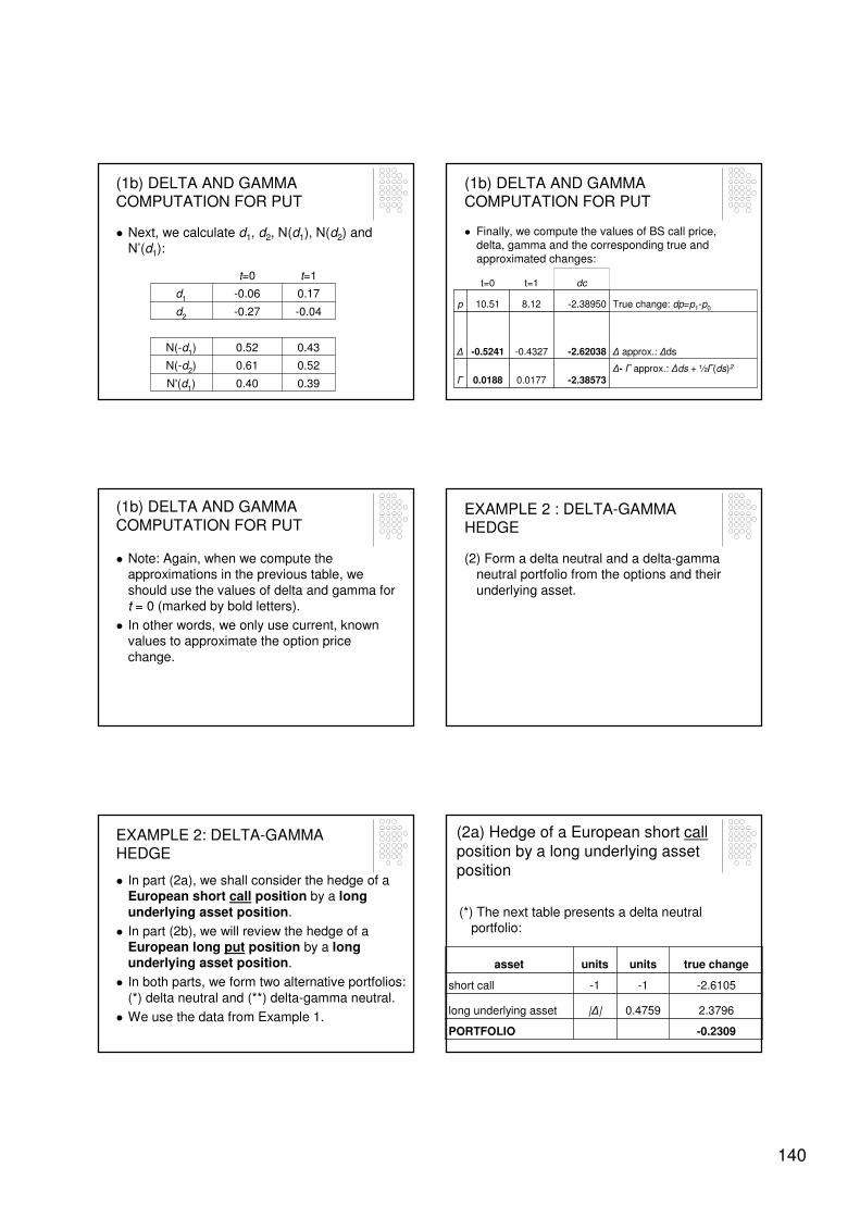
140
(1b) DELTA AND GAMMA COMPUTATION FOR PUT
� Next, we calculate d1, d2, N(d1), N(d2) and N’(d1):
0.390.40N'(d1)
0.520.61N(-d2)
0.430.52N(-d1)
-0.04-0.27d2
0.17-0.06d1
t=1t=0
(1b) DELTA AND GAMMA COMPUTATION FOR PUT
� Finally, we compute the values of BS call price, delta, gamma and the corresponding true and approximated changes:
∆- Γ approx.: ∆ds + ½Γ(ds)2
-2.385730.01770.0188Γ
∆ approx.: ∆ds-2.62038-0.4327-0.5241∆
True change: dp=p1-p0-2.389508.1210.51p
dct=1t=0
(1b) DELTA AND GAMMA
COMPUTATION FOR PUT
� Note: Again, when we compute the approximations in the previous table, we
should use the values of delta and gamma for t = 0 (marked by bold letters).
� In other words, we only use current, known values to approximate the option price
change.
EXAMPLE 2 : DELTA-GAMMA HEDGE
(2) Form a delta neutral and a delta-gamma neutral portfolio from the options and their
underlying asset.
EXAMPLE 2: DELTA-GAMMA HEDGE
� In part (2a), we shall consider the hedge of a European short call position by a long underlying asset position.
� In part (2b), we will review the hedge of a European long put position by a long underlying asset position.
� In both parts, we form two alternative portfolios:
(*) delta neutral and (**) delta-gamma neutral.
� We use the data from Example 1.
(2a) Hedge of a European short call
position by a long underlying asset
position
(*) The next table presents a delta neutral portfolio:
-0.2309PORTFOLIO
2.37960.4759|∆|long underlying asset
-2.6105-1-1short call
true changeunitsunitsasset
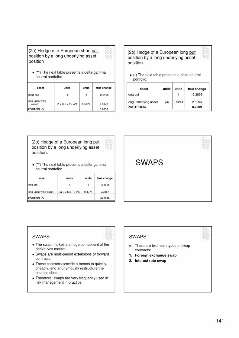
141
� (**) The next table presents a delta-gamma neutral portfolio:
0.0038PORTFOLIO
2.61430.5229|∆ + 0.5 x Γ x dS|long underlying
asset
-2.6105-1-1short call
true changeunitsunitsasset
(2a) Hedge of a European short call
position by a long underlying asset
position
(2b) Hedge of a European long put
position by a long underlying asset
position.
� (*) The next table presents a delta neutral
portfolio:
0.2309PORTFOLIO
2.62040.5241|∆|long underlying asset
-2.389511long put
true changeunitsunitsasset
� (**) The next table presents a delta-gamma neutral portfolio:
-0.0038PORTFOLIO
2.38570.4771|∆ + 0.5 x Γ x dS|long underlying asset
-2.389511long put
true changeunitsunitsasset
(2b) Hedge of a European long put
position by a long underlying asset
position.
SWAPS
SWAPS
� The swap market is a huge component of the derivatives market.
� Swaps are multi-period extensions of forward
contracts.
� These contracts provide a means to quickly,
cheaply, and anonymously restructure the balance sheet.
� Therefore, swaps are very frequently used in
risk management in practice.
SWAPS
� There are two main types of swap contracts:
1. Foreign exchange swap
2. Interest rate swap
142
FOREIGN EXCHANGE SWAP
SWAPS - Foreign exchange swap
� Rather than agreeing to exchange two currencies at forward price at one single future date, a foreign exchange swap (FES)is an exchange of two currencies at a fixed exchange rate on several future dates.
� This fixed exchange rate is called swap rate.
� Thus, FES is a sequence of currency futures contracts.
SWAPS - Foreign exchange swap
Example:
� Two parties might exchange USD 2 million for GBP 1 million in each of the next 5 years.
� In this swap, the USD/GBP exchange rate is fixed for 5 years at 1 GBP = 2 USD that is
USD/GBP = 0.5.
� Let F* = 0.5 USD/GBP denote this constant exchange rate called swap rate.
SWAPS - Foreign exchange swap
� The investor receiving GBP is going to receive GBP 1 million in each of the next 5
years.
� Similarly, the investor receiving USD is going to receive USD 2 million in each of the next 5 years.
SWAPS - Foreign exchange swap
� We shall investigate whether the F* = 0.5 USD/GBP swap rate in this example is a
correct value or not.
� In order to find the fair swap rate, F* we
exploit the analogy between a swap agreement and a sequence of futures
contracts.
SWAPS - Foreign exchange
swap
� The fair value of F* in a T-period swap is given by the next formula:
where Ft denotes the futures exchange rate for date t and yt denotes the risk-free rate for
date t.
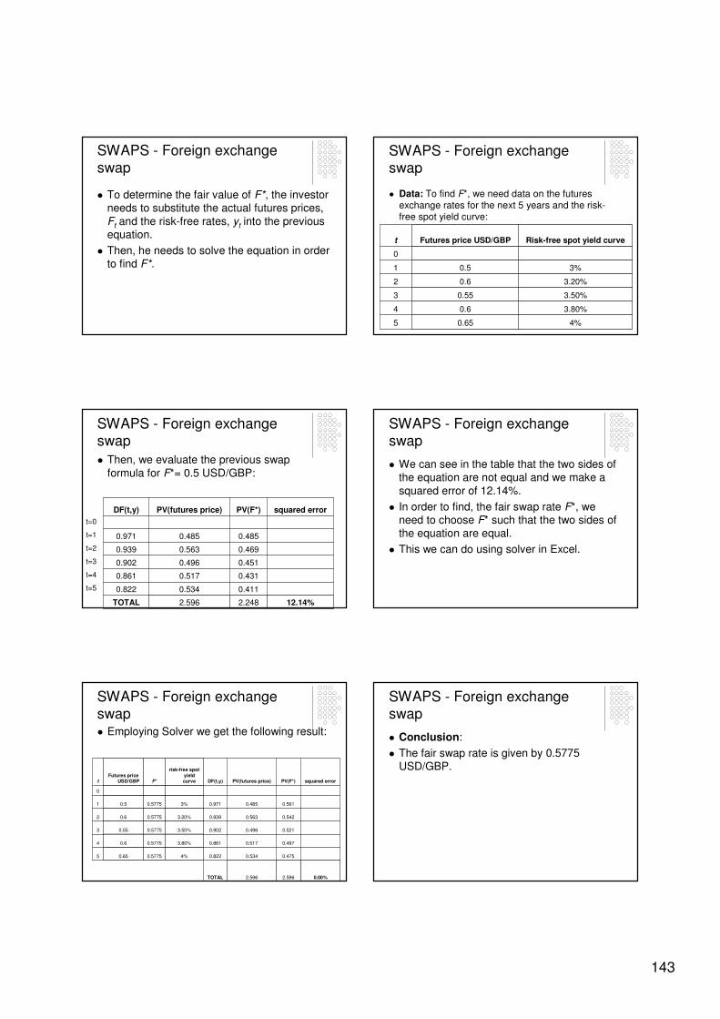
143
SWAPS - Foreign exchange
swap
� To determine the fair value of F*, the investor needs to substitute the actual futures prices,
Ft and the risk-free rates, yt into the previous equation.
� Then, he needs to solve the equation in order to find F*.
SWAPS - Foreign exchange swap
� Data: To find F*, we need data on the futures exchange rates for the next 5 years and the risk-free spot yield curve:
4%0.655
3.80%0.64
3.50%0.553
3.20%0.62
3%0.51
0
Risk-free spot yield curveFutures price USD/GBPt
SWAPS - Foreign exchange swap
� Then, we evaluate the previous swap
formula for F*= 0.5 USD/GBP:
12.14%2.2482.596TOTAL
0.4110.5340.822
0.4310.5170.861
0.4510.4960.902
0.4690.5630.939
0.4850.4850.971
squared errorPV(F*)PV(futures price)DF(t,y)
t=0
t=1
t=2
t=3
t=4
t=5
SWAPS - Foreign exchange swap
� We can see in the table that the two sides of the equation are not equal and we make a
squared error of 12.14%.
� In order to find, the fair swap rate F*, we need to choose F* such that the two sides of the equation are equal.
� This we can do using solver in Excel.
SWAPS - Foreign exchange swap� Employing Solver we get the following result:
0.00%2.5962.596TOTAL
0.4750.5340.8224%0.57750.655
0.4970.5170.8613.80%0.57750.64
0.5210.4960.9023.50%0.57750.553
0.5420.5630.9393.20%0.57750.62
0.5610.4850.9713%0.57750.51
0
squared errorPV(F*)PV(futures price)DF(t,y)
risk-free spot yield curveF*
Futures price USD/GBPt
SWAPS - Foreign exchange swap
� Conclusion:
� The fair swap rate is given by 0.5775 USD/GBP.
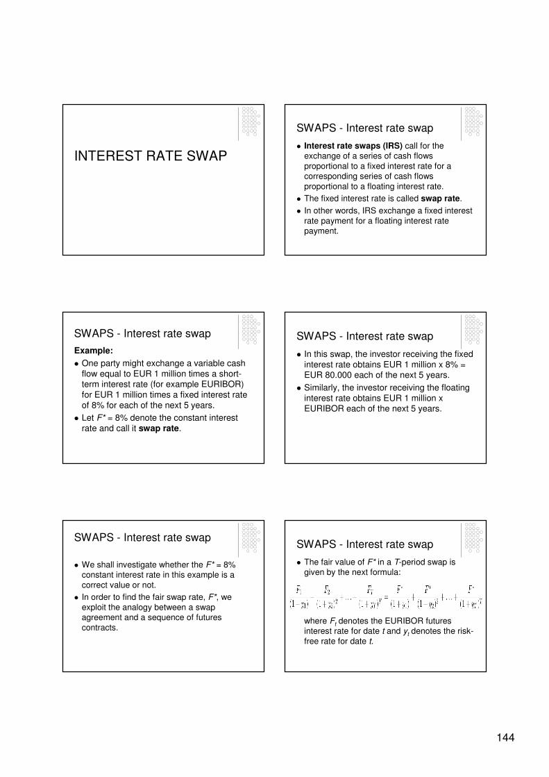
144
INTEREST RATE SWAP
SWAPS - Interest rate swap
� Interest rate swaps (IRS) call for the exchange of a series of cash flows
proportional to a fixed interest rate for a corresponding series of cash flows
proportional to a floating interest rate.
� The fixed interest rate is called swap rate.
� In other words, IRS exchange a fixed interest
rate payment for a floating interest rate payment.
SWAPS - Interest rate swap
Example:
� One party might exchange a variable cash
flow equal to EUR 1 million times a short-term interest rate (for example EURIBOR)
for EUR 1 million times a fixed interest rate
of 8% for each of the next 5 years.
� Let F* = 8% denote the constant interest
rate and call it swap rate.
SWAPS - Interest rate swap
� In this swap, the investor receiving the fixed
interest rate obtains EUR 1 million x 8% = EUR 80.000 each of the next 5 years.
� Similarly, the investor receiving the floating
interest rate obtains EUR 1 million x EURIBOR each of the next 5 years.
SWAPS - Interest rate swap
� We shall investigate whether the F* = 8% constant interest rate in this example is a
correct value or not.
� In order to find the fair swap rate, F*, we
exploit the analogy between a swap agreement and a sequence of futures
contracts.
SWAPS - Interest rate swap
� The fair value of F* in a T-period swap is given by the next formula:
where Ft denotes the EURIBOR futures interest rate for date t and yt denotes the risk-
free rate for date t.
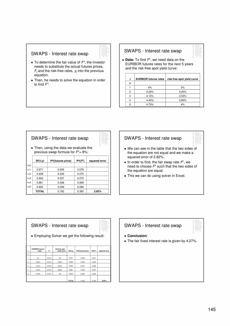
145
SWAPS - Interest rate swap
� To determine the fair value of F*, the investor needs to substitute the actual futures prices,
Ft and the risk-free rates, yt into the previous equation.
� Then, he needs to solve the equation in order to find F*.
SWAPS - Interest rate swap
� Data: To find F*, we need data on the
EURIBOR futures rates for the next 5 years and the risk-free spot yield curve:
4%4.70%5
3.80%4.40%4
3.50%4.10%3
3.20%4.20%2
3%4%1
0
risk-free spot yield curveEURIBOR futures ratest
SWAPS - Interest rate swap
� Then, using the data we evaluate the previous swap formula for F*= 8%:
2.82%0.3600.192TOTAL
0.0660.0390.822
0.0690.0380.861
0.0720.0370.902
0.0750.0390.939
0.0780.0390.971
squared errorPV(F*)PV(futures price)DF(t,y)
t=0
t=1
t=2
t=3
t=4
t=5
SWAPS - Interest rate swap
� We can see in the table that the two sides of the equation are not equal and we make a
squared error of 2.82%.
� In order to find, the fair swap rate F*, we need to choose F* such that the two sides of the equation are equal.
� This we can do using solver in Excel.
SWAPS - Interest rate swap
� Employing Solver we get the following result:
0.00%0.1920.192TOTAL
0.0350.0390.8224%4.27%4.70%5
0.0370.0380.8613.80%4.27%4.40%4
0.0380.0370.9023.50%4.27%4.10%3
0.0400.0390.9393.20%4.27%4.20%2
0.0410.0390.9713%4.27%4%1
0
squared errorPV(F*)PV(futures price)DF(t,y)risk-free spot
yield curveF*EURIBOR futures
ratest
SWAPS - Interest rate swap
� Conclusion:
� The fair fixed interest rate is given by 4.27%.