Embed Size (px)
Citation preview
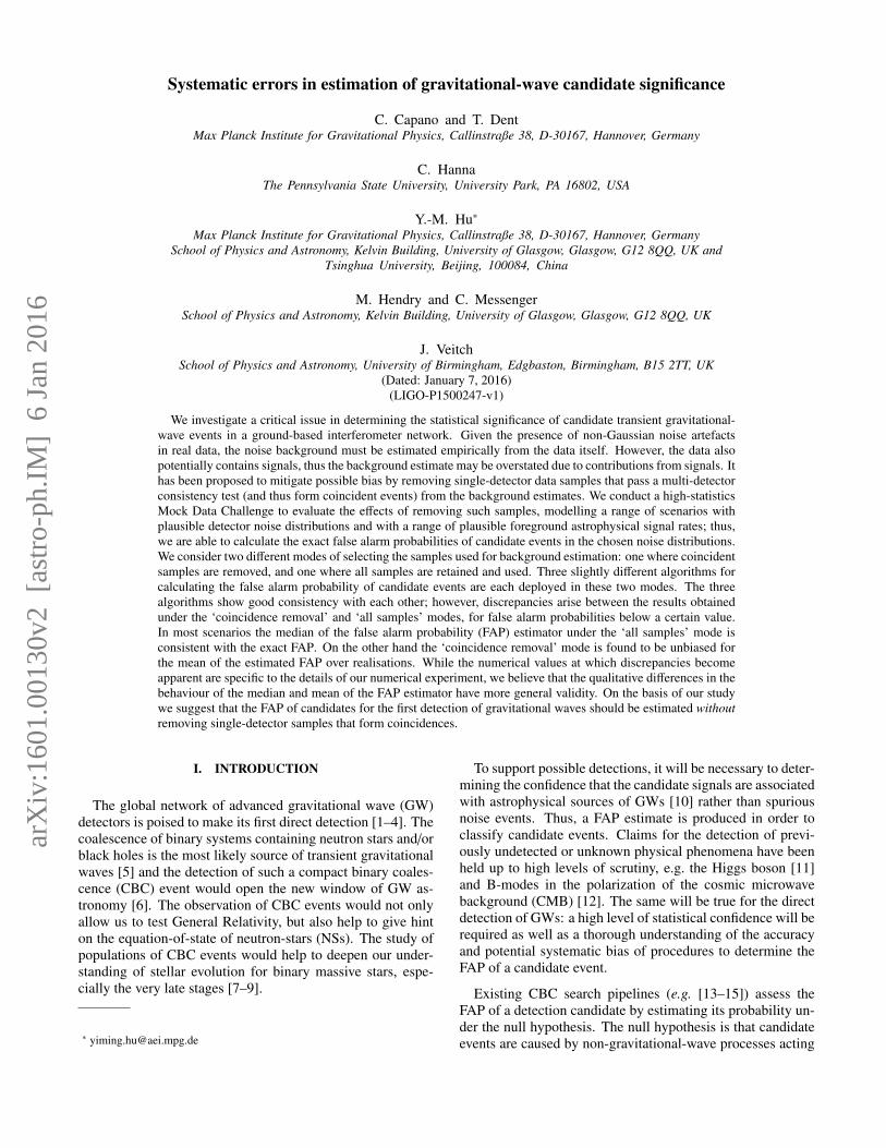
Systematic errors in estimation of gravitational-wave candidate significance
C. Capano and T. DentMax Planck Institute for Gravitational Physics, Callinstraße 38, D-30167, Hannover, Germany
C. HannaThe Pennsylvania State University, University Park, PA 16802, USA
Y.-M. Hu∗Max Planck Institute for Gravitational Physics, Callinstraße 38, D-30167, Hannover, Germany
School of Physics and Astronomy, Kelvin Building, University of Glasgow, Glasgow, G12 8QQ, UK andTsinghua University, Beijing, 100084, China
M. Hendry and C. MessengerSchool of Physics and Astronomy, Kelvin Building, University of Glasgow, Glasgow, G12 8QQ, UK
J. VeitchSchool of Physics and Astronomy, University of Birmingham, Edgbaston, Birmingham, B15 2TT, UK
(Dated: January 7, 2016)(LIGO-P1500247-v1)
We investigate a critical issue in determining the statistical significance of candidate transient gravitational-wave events in a ground-based interferometer network. Given the presence of non-Gaussian noise artefactsin real data, the noise background must be estimated empirically from the data itself. However, the data alsopotentially contains signals, thus the background estimate may be overstated due to contributions from signals. Ithas been proposed to mitigate possible bias by removing single-detector data samples that pass a multi-detectorconsistency test (and thus form coincident events) from the background estimates. We conduct a high-statisticsMock Data Challenge to evaluate the effects of removing such samples, modelling a range of scenarios withplausible detector noise distributions and with a range of plausible foreground astrophysical signal rates; thus,we are able to calculate the exact false alarm probabilities of candidate events in the chosen noise distributions.We consider two different modes of selecting the samples used for background estimation: one where coincidentsamples are removed, and one where all samples are retained and used. Three slightly different algorithms forcalculating the false alarm probability of candidate events are each deployed in these two modes. The threealgorithms show good consistency with each other; however, discrepancies arise between the results obtainedunder the ‘coincidence removal’ and ‘all samples’ modes, for false alarm probabilities below a certain value.In most scenarios the median of the false alarm probability (FAP) estimator under the ‘all samples’ mode isconsistent with the exact FAP. On the other hand the ‘coincidence removal’ mode is found to be unbiased forthe mean of the estimated FAP over realisations. While the numerical values at which discrepancies becomeapparent are specific to the details of our numerical experiment, we believe that the qualitative differences in thebehaviour of the median and mean of the FAP estimator have more general validity. On the basis of our studywe suggest that the FAP of candidates for the first detection of gravitational waves should be estimated withoutremoving single-detector samples that form coincidences.
I. INTRODUCTION
The global network of advanced gravitational wave (GW)detectors is poised to make its first direct detection [1–4]. Thecoalescence of binary systems containing neutron stars and/orblack holes is the most likely source of transient gravitationalwaves [5] and the detection of such a compact binary coales-cence (CBC) event would open the new window of GW as-tronomy [6]. The observation of CBC events would not onlyallow us to test General Relativity, but also help to give hinton the equation-of-state of neutron-stars (NSs). The study ofpopulations of CBC events would help to deepen our under-standing of stellar evolution for binary massive stars, espe-cially the very late stages [7–9].
To support possible detections, it will be necessary to deter-mining the confidence that the candidate signals are associatedwith astrophysical sources of GWs [10] rather than spuriousnoise events. Thus, a FAP estimate is produced in order toclassify candidate events. Claims for the detection of previ-ously undetected or unknown physical phenomena have beenheld up to high levels of scrutiny, e.g. the Higgs boson [11]and B-modes in the polarization of the cosmic microwavebackground (CMB) [12]. The same will be true for the directdetection of GWs: a high level of statistical confidence will berequired as well as a thorough understanding of the accuracyand potential systematic bias of procedures to determine theFAP of a candidate event.
Existing CBC search pipelines (e.g. [13–15]) assess theFAP of a detection candidate by estimating its probability un-der the null hypothesis. The null hypothesis is that candidateevents are caused by non-gravitational-wave processes acting
arX
iv:1
601.
0013
0v2
[as
tro-
ph.I
M]
6 J
an 2
016
2
on and within the interferometers. In order to determine thisprobability, we assign a test statistic value to every possibleresult of a given observation or experiment performed on thedata: larger values indicate a higher deviation from expecta-tions under the null hypothesis. We compute the FAP as theprobability of obtaining a value of the test statistic equal to, orlarger than, the one actually obtained in the experiment. Thesmaller this probability, the more significant is the candidate.
In general the detector output data streams are the sumof terms due to non-astrophysical processes, known as back-ground noise, and of astrophysical GW signals, labelled fore-ground. If we were able to account for all contributions tonoise using predictive and reliable physical models, we wouldthen obtain an accurate calculation of the FAP of any ob-servation. However, for real GW detectors, in addition toterms from known and well-modelled noise processes, thedata contains large numbers of non-Gaussian noise transients(“glitches”, see for example [16, 17]) whose sources are ei-ther unknown or not accurately modelled, and which have po-tentially large effects on searches for transient GWs. Evengiven all the information available from environmental andauxiliary monitor channels at the detectors, many such noisetransients cannot be predicted with sufficient accuracy to ac-count for their effects on search algorithms. Thus, for transientsearches in real detector noise it is necessary to determine thebackground noise distributions empirically, i.e. directly fromthe strain data.
Using the data to empirically estimate the background hasnotable potential drawbacks. It is not possible to operate GWdetectors so as to ‘turn off’ the astrophysical foreground andsimply measure the background; if the detector is operationalthen it is always subject to both background and foregroundsources. In addition, our knowledge of the background noisedistribution is limited by the finite amount of data available.This limitation applies especially in the interesting region oflow event probability under the noise hypothesis, correspond-ing to especially rare noise events.
CBC signals are expected to be well modelled by the pre-dictions of Einstein’s general relativity [18]. The detector dataare cross-correlated (or matched filtered) [19] against a bankof template CBC waveforms, resulting in an signal-to-noiseratio (SNR) time series for each template [20]. If this timeseries crosses a predetermined threshold, the peak value andthe time of the peak are recorded as a trigger. Since GWspropagate at the speed of light (see e.g. [6]), the arrival timesof signals will differ between detectors by '40 ms or less, i.e.Earth’s light crossing time. Differences in arrival times aregoverned by the direction of the source on the sky in relationto the geographical detector locations. We are thus able to im-mediately eliminate the great majority of background noise byrejecting any triggers which are not coincident in two or moredetectors within a predefined coincidence time window givenby the maximum light travel time plus trigger timing errorsdue to noise. Only triggers coincident in multiple detectorswith consistent physical parameters such as binary compo-nent masses are considered as candidate detections. In orderto make a confident detection claim one needs to estimate therarity, i.e., the FAP of an event, and claim detection only when
the probability of an equally loud event being caused by noiseis below a chosen threshold.
The standard approach used in GW data analysis for esti-mating the statistical properties of the background is via anal-ysis of time-shifted data, known as “time slides” [21, 22]. Thismethod exploits the coincidence requirement of foregroundevents by time-shifting the data from one detector relativeto another. Such a shift, if larger than the coincidence win-dow, would prevent a zero-lag signal remaining untouched ina time-shifted analysis. Therefore, from a single time-shiftedanalysis (“time slide”) the output coincident events shouldrepresent one realisation of the background distribution of co-incident events, given the sets of single-detector triggers, as-suming that the background distributions are not correlatedbetween detectors. By performing many time slide analy-ses with different relative time shifts we may accumulate in-stances of background coincidences and thus estimate theirrate and distribution.
The time-slides approach has been an invaluable tool in theanalysis and classification of candidate GW events in the ini-tial detector era. Initial LIGO made no detections, howevernote that in 2010, the LSC (LIGO Scientific Collaboration)and Virgo collaborations (LVC) performed a blind injectionchallenge [10] to check the robustness and confidence of thepipeline. A signal was injected in “hardware” (by actuatingthe test masses) in the global network of interferometers andanalysed by the collaboration knowing only that there was thepossibility of such an artificial event. The blind injection wasrecovered by the templated binary inspiral search with a highsignificance [26]; however, the blind injection exercise high-lighted potential issues with the use of time-shifted analysisto estimate backgrounds in the presence of astrophysical (orsimulated) signals.
Simply time-shifting detector outputs with respect to eachother does not eliminate the possibility of coincident eventsresulting from foreground (signal) triggers from one detectorpassing the coincidence test with random noise triggers in an-other detector. Thus, the ensemble of samples generated bytime-shifted analysis may be “contaminated” by the presenceof foreground events in single-detector data, compared to theensemble that would result from the noise background alone.The distribution of events caused by astrophysical signals isgenerally quite different from that of noise: it is expectedto have a longer tail towards high values of SNR (or otherevent ranking test-statistic used in search algorithms). Thus,depending on the rate of signals and on the realisation of thesignal process obtained in any given experiment, such contam-ination could considerably bias the estimated background. Ifthe estimated background rate is raised by the presence of sig-nals, the FAP of coincident search events (in non-time-shiftedor “zero-lag” data) may be overestimated, implying a conser-vative bias in the estimated FAP. The expected number offalse detection claims will not increase due to the presence ofsignals in time-slide analyses, however some signals may failto be detected due to an elevated background estimate. 1
1 The reader may ask what a “false detection claim” means if signals are
3
Besides the standard time-shift approach, other backgroundestimation techniques have been developed [15, 23, 24]. Allare variants on one key concept: events that are not coincidentwithin the physically allowed time window cannot be fromthe same foreground source. All therefore use non-coincidenttriggers as proxies for the distribution of background eventsdue to detector noise. Differences between methods occurin implementation, and fall into two categories. In the stan-dard scheme, many time slides are applied to a set of trig-gers from a multi-detector observation and all resultant coin-cidences are retained. We label this the ‘all samples’ modeof operation. Concern about the potential conservative bias ofincluding foreground GW events of astrophysical original inthe time-shifted distribution motivates a modification to thisprocedure: one can instead choose to first identify all coin-cidences between different detectors in zero-lag and excludethem from the subsequent time-slide analysis. We label thisthe ‘coincidence removal’ mode of operation.
In this paper we describe the results of an mock data chal-lenge (MDC) in which participants applied three differentbackground estimation algorithms, each applied to the MDCdata in the two modes of operation described above: the ‘co-incidence removal’ and ‘all samples’ modes. Since some as-pects of the MDC data generation were not fully realistic, thealgorithms were simplified compared to their use on real data;two were based on methods currently in use in the LVC, whilethe third introduces a new approach. The MDC consisted ofsimulated realisations of single-detector triggers – maxima ofmatched filter SNR ρ above a fixed threshold value chosen asρ0 = 5.5. The trigger SNR values were generated accordingto analytically modelled background and foreground distribu-tions unknown to the MDC participants. The background dis-tributions spanned a range of complexity including a realisticInitial detector distribution [25]. The foreground triggers werechosen to model one of the most likely first sources, binaryneutron stars, with an expected detection rate from zero tothe maximum expected for the first Advanced detector scienceruns [5]. Participants were asked to apply their algorithms tothese datasets and report, in both modes, the estimated FAPof the loudest event found in each realisation. The MDC usedanalytic formulae to generate the background distributions; al-though we will not, in reality, have access to such formulae,they allow us to compute an “exact” FAP semi-analytically.We use these exact values, alongside other figures of merit, asa benchmark for comparing the results obtained in the ‘coin-cidence removal’ and ‘all samples’ modes, both within eachbackground estimation algorithm and between the different al-gorithms.
In the following section of this paper we provide details ofthe MDC, describing the background and foreground distri-butions, the data generating procedure, and the “exact” FAPcalculation. In Sec. III we then describe the different methods
present. This refers to cases where the search result contains both fore-ground events, and background events with comparable or higher rankingstatistic values. In particular, if the loudest event in the search is due tobackground a detection claim would be misleading.
of background estimation used in this MDC. We report theresults of the challenge in Sec. IV, comparing and contrast-ing the results obtained from each of the algorithms in eachof their 2 modes of operation. Finally in Sec. V we provide asummary and present our conclusions.
II. THE MOCK DATA CHALLENGE
Our MDC is designed to resolve the question of whether toremove (‘coincidence removal’) or not to remove (‘all sam-ples’) coincident zero-lag events from the data used to esti-mate FAP. Simulated single detector triggers are generatedfrom known background and foreground distributions: chal-lenge participants are then given lists of trigger arrival timesand single detector SNRs. The ranking statistic used for eachcoincident trigger is the combined multi-detector SNR. Thecalculation of FAP could be carried out with any appropriateranking statistic. When applied to real data, different pipelinesmay define their ranking statistics in slightly different ways;in order to make a fair comparison in the challenge we usethe multi-detector SNRs as a simplified ranking statistic. Thecumulative distribution functions (CDFs) of the SNR in eachdetector are described analytically and hidden from the chal-lenge participants. With this analytic form, the challenge de-signers are able to compute the exact FAP at the ranking statis-tic value of the loudest coincident event in each realisation.
The challenge consisted of 14 independent experiments,each with a different foreground and background distributionfor which 105 observational realisations are generated (seesection A). This number is large enough to reach the inter-esting statistics region while computationally feasible. Eachrealisation contained, on average, ∼104 single-detector trig-gers in each of two detectors. A realisation should be con-sidered analogous to a single GW observing run. Participantswere asked to estimate the FAP of the loudest coincident eventin each of the 105 realisations for each experiment. The 14experiments cover a variety of background distributions; theforegrounds differ in that the astrophysical rate ranges be-tween zero, i.e., no events, and a relatively high value cor-responding to ∼3 detections per realisation. Analysis of thedifferences between the estimated and exact FAP values en-able us to quantify the effect of removing coincident zero-lagtriggers in the background estimate, as opposed to retainingall samples. It also allows us to directly compare implementa-tions between different algorithms in each mode of operation.Finally, it allows us to quantify the accuracy and limiting pre-cision of our FAP estimates and thus their uncertainties.
We divide our simulations into three groups according toastrophysical rate, and independently into three groups ac-cording to background distribution complexity (“simple”, “re-alistic” and “extreme”). To this nine combinations we haveappended an additional four simulations, three of which haveexactly the same background distributions as three of the orig-inal nine but contain no signals. The final simulation con-tains a background distribution with a deliberately extendedtail such that the generation of particularly loud backgroundtriggers is possible. The primary properties of each experi-
4
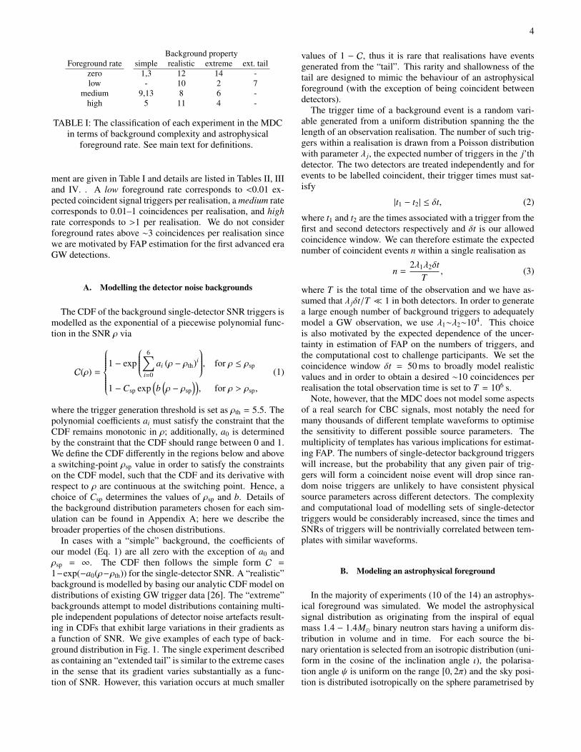
Background propertyForeground rate simple realistic extreme ext. tail
zero 1,3 12 14 -low - 10 2 7
medium 9,13 8 6 -high 5 11 4 -
TABLE I: The classification of each experiment in the MDCin terms of background complexity and astrophysical
foreground rate. See main text for definitions.
ment are given in Table I and details are listed in Tables II, IIIand IV. . A low foreground rate corresponds to <0.01 ex-pected coincident signal triggers per realisation, a medium ratecorresponds to 0.01–1 coincidences per realisation, and highrate corresponds to >1 per realisation. We do not considerforeground rates above ∼3 coincidences per realisation sincewe are motivated by FAP estimation for the first advanced eraGW detections.
A. Modelling the detector noise backgrounds
The CDF of the background single-detector SNR triggers ismodelled as the exponential of a piecewise polynomial func-tion in the SNR ρ via
C(ρ) =
1 − exp
6∑i=0
ai (ρ − ρth)i
, for ρ ≤ ρsp
1 −Csp exp(b(ρ − ρsp
)), for ρ > ρsp,
(1)
where the trigger generation threshold is set as ρth = 5.5. Thepolynomial coefficients ai must satisfy the constraint that theCDF remains monotonic in ρ; additionally, a0 is determinedby the constraint that the CDF should range between 0 and 1.We define the CDF differently in the regions below and abovea switching-point ρsp value in order to satisfy the constraintson the CDF model, such that the CDF and its derivative withrespect to ρ are continuous at the switching point. Hence, achoice of Csp determines the values of ρsp and b. Details ofthe background distribution parameters chosen for each sim-ulation can be found in Appendix A; here we describe thebroader properties of the chosen distributions.
In cases with a “simple” background, the coefficients ofour model (Eq. 1) are all zero with the exception of a0 andρsp = ∞. The CDF then follows the simple form C =
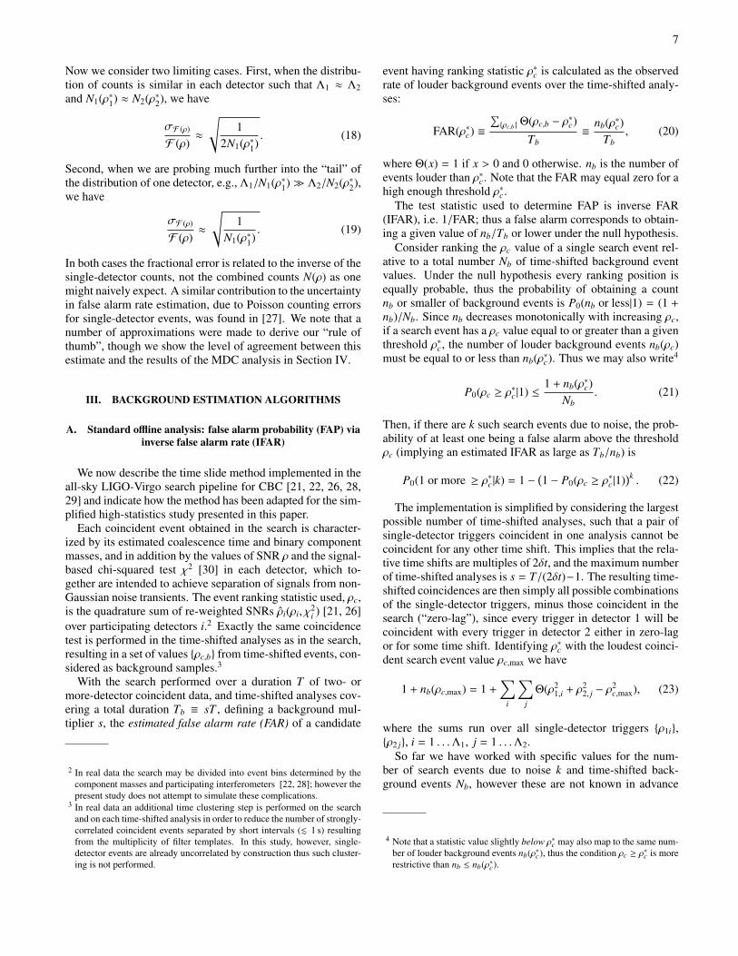
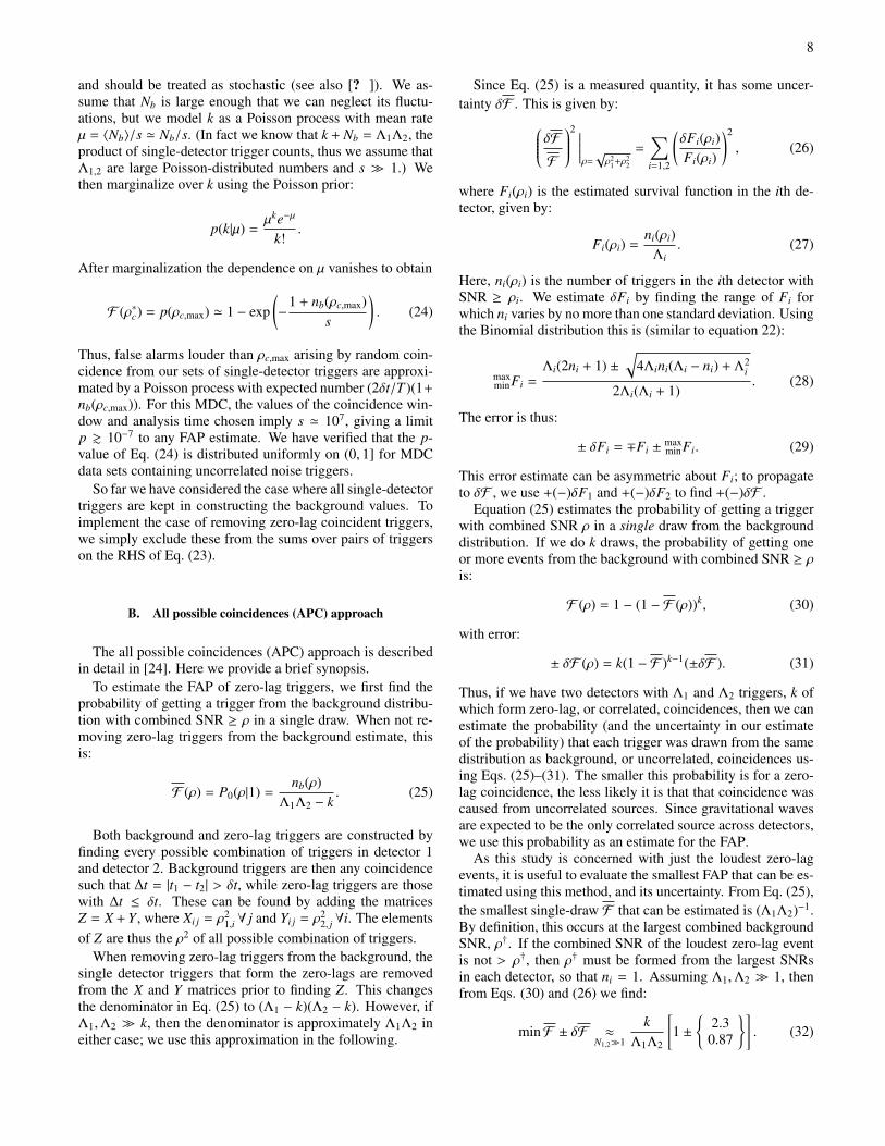
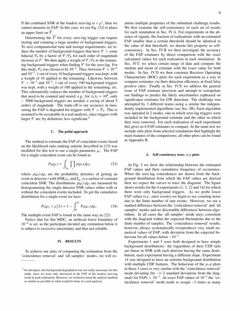
1−exp(−a0(ρ−ρth)) for the single-detector SNR. A “realistic”background is modelled by basing our analytic CDF model ondistributions of existing GW trigger data [26]. The “extreme”backgrounds attempt to model distributions containing multi-ple independent populations of detector noise artefacts result-ing in CDFs that exhibit large variations in their gradients asa function of SNR. We give examples of each type of back-ground distribution in Fig. 1. The single experiment describedas containing an “extended tail” is similar to the extreme casesin the sense that its gradient varies substantially as a func-tion of SNR. However, this variation occurs at much smaller
values of 1 − C, thus it is rare that realisations have eventsgenerated from the “tail”. This rarity and shallowness of thetail are designed to mimic the behaviour of an astrophysicalforeground (with the exception of being coincident betweendetectors).
The trigger time of a background event is a random vari-able generated from a uniform distribution spanning the thelength of an observation realisation. The number of such trig-gers within a realisation is drawn from a Poisson distributionwith parameter λ j, the expected number of triggers in the j’thdetector. The two detectors are treated independently and forevents to be labelled coincident, their trigger times must sat-isfy
|t1 − t2| ≤ δt, (2)
where t1 and t2 are the times associated with a trigger from thefirst and second detectors respectively and δt is our allowedcoincidence window. We can therefore estimate the expectednumber of coincident events n within a single realisation as
n =2λ1λ2δt
T, (3)
where T is the total time of the observation and we have as-sumed that λ jδt/T � 1 in both detectors. In order to generatea large enough number of background triggers to adequatelymodel a GW observation, we use λ1∼λ2∼104. This choiceis also motivated by the expected dependence of the uncer-tainty in estimation of FAP on the numbers of triggers, andthe computational cost to challenge participants. We set thecoincidence window δt = 50 ms to broadly model realisticvalues and in order to obtain a desired ∼10 coincidences perrealisation the total observation time is set to T = 106 s.
Note, however, that the MDC does not model some aspectsof a real search for CBC signals, most notably the need formany thousands of different template waveforms to optimisethe sensitivity to different possible source parameters. Themultiplicity of templates has various implications for estimat-ing FAP. The numbers of single-detector background triggerswill increase, but the probability that any given pair of trig-gers will form a coincident noise event will drop since ran-dom noise triggers are unlikely to have consistent physicalsource parameters across different detectors. The complexityand computational load of modelling sets of single-detectortriggers would be considerably increased, since the times andSNRs of triggers will be nontrivially correlated between tem-plates with similar waveforms.
B. Modeling an astrophysical foreground
In the majority of experiments (10 of the 14) an astrophys-ical foreground was simulated. We model the astrophysicalsignal distribution as originating from the inspiral of equalmass 1.4 − 1.4M� binary neutron stars having a uniform dis-tribution in volume and in time. For each source the bi-nary orientation is selected from an isotropic distribution (uni-form in the cosine of the inclination angle ι), the polarisa-tion angle ψ is uniform on the range [0, 2π) and the sky posi-tion is distributed isotropically on the sphere parametrised by

5
(a) A “simple” example background(experiment 3).
(b) A “realistic” example background(experiment 12).
(c) An “extreme” example background(experiment 14).
FIG. 1: Examples of different background distributions used in the MDC. In each of the three examples we show thecomplementary CDF (1 − C) versus the single-detector SNR for each detector. There were no foreground distributions present
in these experiments.
right ascension α (with range [0, 2π)) and declination δ (range[−π/2, π/2)). Given a set of these parameters we can computethe optimal single-detector SNR ρopt as
ρ2opt = 4
fISCO∫fmin
|h( f )|2
S n( f )d f (4)
where the lower and upper integration limits are selected as10 Hz and as the innermost stable circular orbit frequency= 1570 Hz for our choice of total system mass. The detec-tor noise spectral density S n( f ) corresponds to the advancedLIGO design [2], and the frequency domain signal in the sta-tionary phase approximation is given by
h( f ) =Q({θ})M5/6
d
√524π−2/3 f −7/6eiΨ( f ). (5)
Here the function Q({θ}), where {θ} = (α, δ, ψ, cos ι), describesthe antenna response of the detector; d is the distance to thesource, and M is the “chirp mass” of the system given byM = (m1m2)3/5/(m1+m2)1/5. Since we consider that such sig-nals, if present in the data, are recovered with exactly match-ing templates, the phase term Ψ( f ) does not influence the op-timal SNR of Eq. 4. Hence the square of the observed (ormatched filter) SNR ρ is drawn from a non-central χ2 distri-bution with 2 degrees of freedom and non-centrality parameterequal to ρ2
opt.We generate foreground events within a sphere of radius
1350 Mpc such that an optimally oriented event at the bound-ary has <0.3% probability of producing a trigger with SNR>ρth = 5.5. Each event is given a random location (uniformin volume) and orientation from which we calculate the corre-sponding optimal SNR and relative detector arrival times. Thematched filter SNR is modelled as a draw from the non-centralchi-squared distribution. For each detector, if the matched fil-ter SNR is larger than ρth, independently of the other detector,it is recorded as a single detector trigger. The arrival timein the first detector (chosen as the LIGO Hanford interferom-eter) is randomly selected uniformly within the observation
time and the corresponding time in the second detector (theLIGO Livingston interferometer) is set by the arrival time dif-ference defined by the source sky position. We do not modelstatistical uncertainty in the arrival time measurements, hencewhen a foreground event produces a trigger in both detectorsthe trigger times will necessarily lie within the time windowand will generate a coincident event.
C. The definition of false alarm probability (FAP) for theMDC
In order to define the FAP for any given realisation of anexperiment we require a ranking statistic which is a functionof the coincident triggers within a realisation. In this MDC thechosen ranking statistic was the combined SNR of coincidentevents, defined as
ρ2 = ρ21 + ρ2
2, (6)
where ρ1,2 are the SNRs of the single-detector triggers form-ing the coincident event. Challenge participants were requiredto estimate the FAP of the “loudest” coincident event withineach realisation, i.e. the event having the highest ρ value, in-dependent of its unknown origin (background or foreground).The FAP of an outcome defined by a loudest event ρ∗ is theprobability of obtaining at least one background event hav-ing ρ ≥ ρ∗ within a single realisation. Given that single-detector background distributions fall off with increasing ρ1,2,the louder a coincident event is, the less likely it is for a com-parable or larger ρ value to be generated by noise, and thesmaller the FAP.
With access to the analytical description of the backgroundsfrom both detectors we may compute the single trial FAP F1
6
as
1 − F1(ρ) =
√ρ2−ρ2
th∫ρth
dρ1
√ρ2−ρ2
1∫ρth
dρ2 p1(ρ1)p2(ρ2),
=
√ρ2−ρ2
th∫ρth
dρ1 p1(ρ1)C2
(√ρ2 − ρ2
1
), (7)
where p1(ρ1) and p2(ρ2) are the probability distribution func-tions (PDFs) of the background distributions (obtained by dif-ferentiating the corresponding CDFs with respect to ρ j), andC2(ρ2) is the CDF for the second detector.
To account for the fact that we are interested in the “loud-est” coincident event within each realisation we must performan additional marginalisation over the unknown number ofsuch coincident events. To do this we model the actual num-ber of coincidences as drawn from a Poisson distribution withknown mean n (values for the different MDC experiments aregiven in Table IV). The FAP of the “loudest” event is mod-elled as the probability of obtaining one or more coincidentevents with a combined SNR ≥ ρ and is given by
F (ρ) =
∞∑j=0
(1 − (1 − F1(ρ)) j
) n je−n
j!. (8)
Challenge participants only had access to the trigger ρ1,2 val-ues and trigger times in each realisation and were not given thedistributions from which they were drawn. Estimates of theloudest coincident event FAP F from all participants will becompared to the “exact” values computed according to Eq. 8.
D. The expected error on estimated false alarm probability(FAP)
Inferring the FAP, as defined above, from a finite sample ofdata will have associated uncertainty, i.e., the computed valueswill be approximate. Methods to estimate the FAP at a givencombined SNR value F (ρ) involve counting the number ofnoise events N(ρ) above that value:
N(ρ) =x
ρ≥ρth
n1(ρ1) n2(ρ2) dρ1dρ2
= Λ1Λ2 −
x
ρ<ρth
n1(ρ1) n2(ρ2) dρ1dρ2, (9)
where ni(ρi) is the number density of background triggersfrom detector i and Λi is the total number of background trig-gers from detector i. The region of integration is boundedby a threshold on the coincident SNR statistic of Eq. 6,though in general one may choose other functional forms forρ(ρ1, ρ2, . . . ).
It is possible to compute (either analytically or numerically)the error on N(ρ) given any functional form for ρ. However,we seek a simple “rule of thumb” as a general approximation.We replace the region ρ< ρth with an equivalent hyper-cuboid
with lengths ρ∗i , such that for an event to be counted towardsthe FAP it must have a SNR greater than ρ∗i in either detectors.In this case, the number of louder triggers as a function of ρcan be approximated by
N(ρ) ≈ Λ1Λ2 −
∫ ρ∗1
0dρ1
∫ ρ∗2
0dρ2 n1(ρ1)n2(ρ2)
≈ Λ1Λ2 − N′1(ρ∗1)N′2(ρ∗2), (10)
where
N′i (ρ∗i ) ≡
∫ ρ∗i
0ni(ρi) dρi, (11)
is the cumulative number of triggers from detector i. We thendefine the inferred FAP as
F (ρ) ≈N(ρ)Λ1Λ2
≈ 1 −N′1(ρ∗1)N′2(ρ∗2)
Λ1Λ2(12)
We wish to characterise the error in F (ρ) given the errorin the number of triggers counted above ρi in each detector.We expect that this error will increase when fewer triggers areavailable to estimate the single detector counts. TransformingEq. 12 to use the counts above a threshold ρ∗i in each detectorvia Ni(ρi) ≡ Λi − N′i (ρi), we have
F (ρ) ≈ 1 −(Λ1 − N1(ρ∗1)
)(Λ2 − N2(ρ∗2)
)Λ1Λ2
. (13)
Assuming a negligible error on the total count of triggers ineach detector Λi, we can then write
σ2F (ρ) ≈
∑i
(∂F (ρ)∂Ni(ρ∗i )
)2
σ2Ni(ρ∗i ). (14)
Taking the distribution of counts Ni(ρ) to be Poisson, we havestandard errors σ2
Ni(ρ∗i ) = Ni(ρ∗i ); for the two-detector case wethen find
σ2F (ρ) ≈
(Λ2 − N2(ρ∗2)
)2N1(ρ∗1) +(Λ1 − N1(ρ∗1)
)2N2(ρ∗2)
Λ21Λ2
2
,
(15)
hence the fractional error is
σF (ρ)
F (ρ)≈
√(Λ2−N2(ρ∗2))2
N1(ρ∗1)N22(ρ∗2)
+(Λ1−N1(ρ∗1))2
N2(ρ∗2)N12(ρ∗1)
Λ2N2(ρ∗2) + Λ1
N1(ρ∗1) − 1. (16)
In the limit of low FAPs, N′1(ρ∗1) � Λ1 and N′2(ρ∗1) � Λ2, ourexpression simplifies to
σF (ρ)
F (ρ)≈
√(Λ2
N2(ρ∗2)
)21
N1(ρ∗1) +
(Λ1
N1(ρ∗1)
)21
N2(ρ∗2)
Λ2N2(ρ∗2) + Λ1
N1(ρ∗1)
. (17)
7
Now we consider two limiting cases. First, when the distribu-tion of counts is similar in each detector such that Λ1 ≈ Λ2and N1(ρ∗1) ≈ N2(ρ∗2), we have
σF (ρ)
F (ρ)≈
√1
2N1(ρ∗1). (18)
Second, when we are probing much further into the “tail” ofthe distribution of one detector, e.g., Λ1/N1(ρ∗1) � Λ2/N2(ρ∗2),we have
σF (ρ)
F (ρ)≈
√1
N1(ρ∗1). (19)
In both cases the fractional error is related to the inverse of thesingle-detector counts, not the combined counts N(ρ) as onemight naively expect. A similar contribution to the uncertaintyin false alarm rate estimation, due to Poisson counting errorsfor single-detector events, was found in [27]. We note that anumber of approximations were made to derive our “rule ofthumb”, though we show the level of agreement between thisestimate and the results of the MDC analysis in Section IV.
III. BACKGROUND ESTIMATION ALGORITHMS
A. Standard offline analysis: false alarm probability (FAP) viainverse false alarm rate (IFAR)
We now describe the time slide method implemented in theall-sky LIGO-Virgo search pipeline for CBC [21, 22, 26, 28,29] and indicate how the method has been adapted for the sim-plified high-statistics study presented in this paper.
Each coincident event obtained in the search is character-ized by its estimated coalescence time and binary componentmasses, and in addition by the values of SNR ρ and the signal-based chi-squared test χ2 [30] in each detector, which to-gether are intended to achieve separation of signals from non-Gaussian noise transients. The event ranking statistic used, ρc,is the quadrature sum of re-weighted SNRs ρi(ρi, χ
2i ) [21, 26]
over participating detectors i.2 Exactly the same coincidencetest is performed in the time-shifted analyses as in the search,resulting in a set of values {ρc,b} from time-shifted events, con-sidered as background samples.3
With the search performed over a duration T of two- ormore-detector coincident data, and time-shifted analyses cov-ering a total duration Tb ≡ sT , defining a background mul-tiplier s, the estimated false alarm rate (FAR) of a candidate
2 In real data the search may be divided into event bins determined by thecomponent masses and participating interferometers [22, 28]; however thepresent study does not attempt to simulate these complications.
3 In real data an additional time clustering step is performed on the searchand on each time-shifted analysis in order to reduce the number of strongly-correlated coincident events separated by short intervals (. 1 s) resultingfrom the multiplicity of filter templates. In this study, however, single-detector events are already uncorrelated by construction thus such cluster-ing is not performed.
event having ranking statistic ρ∗c is calculated as the observedrate of louder background events over the time-shifted analy-ses:
FAR(ρ∗c) ≡
∑{ρc,b}
Θ(ρc,b − ρ∗c)
Tb≡
nb(ρ∗c)Tb
, (20)
where Θ(x) = 1 if x > 0 and 0 otherwise. nb is the number ofevents louder than ρ∗c. Note that the FAR may equal zero for ahigh enough threshold ρ∗c.
The test statistic used to determine FAP is inverse FAR(IFAR), i.e. 1/FAR; thus a false alarm corresponds to obtain-ing a given value of nb/Tb or lower under the null hypothesis.
Consider ranking the ρc value of a single search event rel-ative to a total number Nb of time-shifted background eventvalues. Under the null hypothesis every ranking position isequally probable, thus the probability of obtaining a countnb or smaller of background events is P0(nb or less|1) = (1 +
nb)/Nb. Since nb decreases monotonically with increasing ρc,if a search event has a ρc value equal to or greater than a giventhreshold ρ∗c, the number of louder background events nb(ρc)must be equal to or less than nb(ρ∗c). Thus we may also write4
P0(ρc ≥ ρ∗c |1) ≤
1 + nb(ρ∗c)Nb
. (21)
Then, if there are k such search events due to noise, the prob-ability of at least one being a false alarm above the thresholdρc (implying an estimated IFAR as large as Tb/nb) is
P0(1 or more ≥ ρ∗c |k) = 1 −(1 − P0(ρc ≥ ρ
∗c |1)
)k . (22)
The implementation is simplified by considering the largestpossible number of time-shifted analyses, such that a pair ofsingle-detector triggers coincident in one analysis cannot becoincident for any other time shift. This implies that the rela-tive time shifts are multiples of 2δt, and the maximum numberof time-shifted analyses is s = T/(2δt)−1. The resulting time-shifted coincidences are then simply all possible combinationsof the single-detector triggers, minus those coincident in thesearch (“zero-lag”), since every trigger in detector 1 will becoincident with every trigger in detector 2 either in zero-lagor for some time shift. Identifying ρ∗c with the loudest coinci-dent search event value ρc,max we have
1 + nb(ρc,max) = 1 +∑
i
∑j
Θ(ρ21,i + ρ2
2, j − ρ2c,max), (23)
where the sums run over all single-detector triggers {ρ1i},{ρ2 j}, i = 1 . . .Λ1, j = 1 . . .Λ2.
So far we have worked with specific values for the num-ber of search events due to noise k and time-shifted back-ground events Nb, however these are not known in advance
4 Note that a statistic value slightly below ρ∗c may also map to the same num-ber of louder background events nb(ρ∗c), thus the condition ρc ≥ ρ
∗c is more
restrictive than nb ≤ nb(ρ∗c).
8
and should be treated as stochastic (see also [? ]). We as-sume that Nb is large enough that we can neglect its fluctu-ations, but we model k as a Poisson process with mean rateµ = 〈Nb〉/s ' Nb/s. (In fact we know that k + Nb = Λ1Λ2, theproduct of single-detector trigger counts, thus we assume thatΛ1,2 are large Poisson-distributed numbers and s � 1.) Wethen marginalize over k using the Poisson prior:
p(k|µ) =µke−µ
k!.
After marginalization the dependence on µ vanishes to obtain
F (ρ∗c) = p(ρc,max) ' 1 − exp(−
1 + nb(ρc,max)s
). (24)
Thus, false alarms louder than ρc,max arising by random coin-cidence from our sets of single-detector triggers are approxi-mated by a Poisson process with expected number (2δt/T )(1+
nb(ρc,max)). For this MDC, the values of the coincidence win-dow and analysis time chosen imply s ' 107, giving a limitp & 10−7 to any FAP estimate. We have verified that the p-value of Eq. (24) is distributed uniformly on (0, 1] for MDCdata sets containing uncorrelated noise triggers.
So far we have considered the case where all single-detectortriggers are kept in constructing the background values. Toimplement the case of removing zero-lag coincident triggers,we simply exclude these from the sums over pairs of triggerson the RHS of Eq. (23).
B. All possible coincidences (APC) approach
The all possible coincidences (APC) approach is describedin detail in [24]. Here we provide a brief synopsis.
To estimate the FAP of zero-lag triggers, we first find theprobability of getting a trigger from the background distribu-tion with combined SNR ≥ ρ in a single draw. When not re-moving zero-lag triggers from the background estimate, thisis:
F (ρ) = P0(ρ|1) =nb(ρ)
Λ1Λ2 − k. (25)
Both background and zero-lag triggers are constructed byfinding every possible combination of triggers in detector 1and detector 2. Background triggers are then any coincidencesuch that ∆t = |t1 − t2| > δt, while zero-lag triggers are thosewith ∆t ≤ δt. These can be found by adding the matricesZ = X + Y , where Xi j = ρ2
1,i ∀ j and Yi j = ρ22, j ∀i. The elements
of Z are thus the ρ2 of all possible combination of triggers.When removing zero-lag triggers from the background, the
single detector triggers that form the zero-lags are removedfrom the X and Y matrices prior to finding Z. This changesthe denominator in Eq. (25) to (Λ1 − k)(Λ2 − k). However, ifΛ1,Λ2 � k, then the denominator is approximately Λ1Λ2 ineither case; we use this approximation in the following.
Since Eq. (25) is a measured quantity, it has some uncer-tainty δF . This is given by:δF
F
2 ∣∣∣∣∣ρ=√ρ2
1+ρ22
=∑i=1,2
(δFi(ρi)Fi(ρi)
)2
, (26)
where Fi(ρi) is the estimated survival function in the ith de-tector, given by:
Fi(ρi) =ni(ρi)
Λi. (27)
Here, ni(ρi) is the number of triggers in the ith detector withSNR ≥ ρi. We estimate δFi by finding the range of Fi forwhich ni varies by no more than one standard deviation. Usingthe Binomial distribution this is (similar to equation 22):
maxminFi =
Λi(2ni + 1) ±√
4Λini(Λi − ni) + Λ2i
2Λi(Λi + 1). (28)
The error is thus:
± δFi = ∓Fi ±maxminFi. (29)
This error estimate can be asymmetric about Fi; to propagateto δF , we use +(−)δF1 and +(−)δF2 to find +(−)δF .
Equation (25) estimates the probability of getting a triggerwith combined SNR ρ in a single draw from the backgrounddistribution. If we do k draws, the probability of getting oneor more events from the background with combined SNR ≥ ρis:
F (ρ) = 1 − (1 − F (ρ))k, (30)
with error:
± δF (ρ) = k(1 − F )k−1(±δF ). (31)
Thus, if we have two detectors with Λ1 and Λ2 triggers, k ofwhich form zero-lag, or correlated, coincidences, then we canestimate the probability (and the uncertainty in our estimateof the probability) that each trigger was drawn from the samedistribution as background, or uncorrelated, coincidences us-ing Eqs. (25)–(31). The smaller this probability is for a zero-lag coincidence, the less likely it is that that coincidence wascaused from uncorrelated sources. Since gravitational wavesare expected to be the only correlated source across detectors,we use this probability as an estimate for the FAP.
As this study is concerned with just the loudest zero-lagevents, it is useful to evaluate the smallest FAP that can be es-timated using this method, and its uncertainty. From Eq. (25),the smallest single-draw F that can be estimated is (Λ1Λ2)−1.By definition, this occurs at the largest combined backgroundSNR, ρ†. If the combined SNR of the loudest zero-lag eventis not > ρ†, then ρ† must be formed from the largest SNRsin each detector, so that ni = 1. Assuming Λ1,Λ2 � 1, thenfrom Eqs. (30) and (26) we find:
minF ± δF ≈N1,2�1
kΛ1Λ2
[1 ±
{2.30.87
}]. (32)
9
If the combined SNR of the loudest zero-lag is > ρ†, then wecannot measure its FAP. In this case, we use Eq. (32) to placean upper limit on F .
Determining the F for every zero-lag trigger can requirestoring and counting a large number of background triggers.To save computational time and storage requirements, we re-duce the number of background triggers that have F > somefiducial F0 by a factor of F /F0 for each order of magnitudeincrease in F . We then apply a weight of F /F0 to the remain-ing background triggers when finding F for the zero-lag. Forthis study, F0 was chosen to be 10−5. Thus, between F = 10−4
and 10−5, 1 out of every 10 background triggers was kept, witha weight of 10 applied to the remaining. Likewise, betweenF = 10−3 and 10−2, 1 out of every 100 background triggerswas kept, with a weight of 100 applied to the remaining; etc.This substantially reduces the number of background triggersthat need to be counted and stored; e.g., for λ1λ2 = 108, only∼ 5000 background triggers are needed, a saving of about 5orders of magnitude. The trade-off is our accuracy in mea-suring the FAP is degraded for triggers with F > F0. This isassumed to be acceptable in a real analysis, since triggers withlarger F are, by definition, less significant.5
C. The gstlal approach
The method to estimate the FAP of coincident events basedon the likelihood ratio ranking statistic described in [15] wasmodified for this test to use a single parameter, ρc. The FAPfor a single coincident event can be found as
P0(ρc) =
∫Σρc
∏i
p(ρi) dρi, (33)
where p(ρi) dρi are the probability densities of getting anevent in detector i with SNR ρi, and Σρc is a surface of constantcoincident SNR. The distributions p(ρi) dρi are measured byhistogramming the single detector SNR values either with orwithout the coincident events included. To get the cumulativedistribution for a single event we have
P0(ρc > ρ∗c |1) = 1 −
∫ ρ∗c
0P0(ρc) dρc. (34)
The multiple event FAP is found in the same way as (22).Notice that for this MDC, an artificial lower boundary of
10−6 is set, as the participant decided any estimation below itis subject to excessive uncertainty and thus not reliable.
IV. RESULTS
To achieve our aims of comparing the estimation from the‘coincidence removal’ and ‘all samples’ modes, we will ex-
5 In retrospect, this background degradation was not really necessary for thisstudy, since we were only interested in the FAP of the loudest zero-lagevent in each realisation. However, we wished to keep the analysis methodas similar as possible to what would be done in a real analysis.
amine multiple properties of the submitted challenge results.We first examine the self-consistency of each set of resultsfor each simulation in Sec. IV A. For experiments in the ab-sence of signals, the fraction of realisations with an estimatedFAP smaller than a certain threshold should be identical tothe value of that threshold; we denote this property as self-consistency. In Sec. IV B we then investigate the accuracyof the FAP estimates by direct comparison with the exactcalculated values for each realisation in each simulation. InSec. IV C we select certain range of data and compare themedian and mean of estimate with the exact value for bothmodes. In Sec. IV D we then construct Receiver OperatingCharacteristic (ROC) plots for each experiment as a way tocompare estimates via their detection efficiency at fixed falsepositive rates. Finally in Sec. IV E we address the generalissue of FAP estimate precision and attempt to extrapolateour findings to predict the likely uncertainties rephrased onsignificance estimates for GW detection. The challenge wasattempted by 3 different teams using a similar but indepen-dently implemented algorithms (see Sec. III). Each algorithmwas operated in 2 modes, one in which zero-lag triggers wereincluded in the background estimate and the other in whichthey were removed. For each realisation of each experimentthis gives us 6 FAP estimates to compare. In the main text weinclude only plots from selected simulations that highlight themain features of the comparisons; all other plots can be foundin Appendix B.
A. Self consistency tests: p-p plots
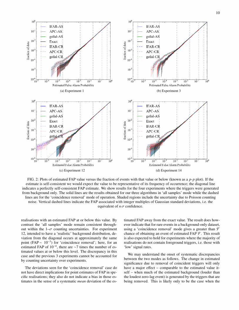
In Fig. 2 we show the relationship between the estimatedFAP values and their cumulative frequency of occurrence.When the zero-lag coincidences are drawn from the back-ground distribution from which the FAP values are derivedthen we expect the curves to trace the diagonal. The figureshows results for the 4 experiments (1, 3, 12 and 14) for whichthere were only background triggers. As we probe lowerFAP values (i.e., rarer events) we begin to see counting noisedue to the finite number of rare events. However, we see amarked difference between the ‘coincidence removal’ and ‘allsamples’ modes and no discernible differences between algo-rithms. In all cases the ‘all samples’ mode stays consistentwith the diagonal within the expected fluctuations due to thefinite number of samples. The ‘coincidence removal’ results,however, always systematically overproduces very small nu-merical values of FAP, with deviation from the expected be-haviour for all values below ∼10−3.
Experiments 1 and 3 were both designed to have simplebackground distributions: the logarithms of their CDF tailsare linear in SNR with each detector having the same distri-bution, each experiment having a different slope. Experiment14 was designed to have an extreme background distributionwith multiple CDF features. The behaviour of the p–p plotsin these 3 cases is very similar with the ‘coincidence removal’mode deviating (by ∼1–2 standard deviations from the diag-onal) for FAPs < 10−3. At exact FAP values of 10−4 the ‘co-incidence removal’ mode tends to assign ∼3 times as many
10
(a) Experiment 1 (b) Experiment 3
(c) Experiment 12 (d) Experiment 14
FIG. 2: Plots of estimated FAP value versus the fraction of events with that value or below (known as a p-p plot). If theestimate is self-consistent we would expect the value to be representative of its frequency of occurrence; the diagonal line
indicates a perfectly self-consistent FAP estimate. We show results for the four experiments where the triggers were generatedfrom background only. The solid lines are the results obtained for our three algorithms in ‘all samples’ mode while the dashed
lines are for the ‘coincidence removal’ mode of operation. Shaded regions include the uncertainty due to Poisson countingnoise. Vertical dashed lines indicate the FAP associated with integer multiples of Gaussian standard deviations, i.e. the
equivalent of nσ confidence.
realisations with an estimated FAP at or below this value. Bycontrast the ‘all samples’ mode remain consistent through-out within the 1–σ counting uncertainties. For experiment12, intended to have a ‘realistic’ background distribution, de-viation from the diagonal occurs at approximately the samepoint (FAP∼ 10−3) for ‘coincidence removal’; here, for anestimated FAP of 10−4, there are ∼7 times the number of es-timated values at or below this level. The discrepancy in thiscase and the previous 3 experiments cannot be accounted forby counting uncertainty over experiments.
The deviations seen for the ‘coincidence removal’ case donot have direct implications for point estimates of FAP in spe-cific realisations; they also do not indicate a bias in those es-timates in the sense of a systematic mean deviation of the es-
timated FAP away from the exact value. The result does how-ever indicate that for rare events in a background-only dataset,using a ‘coincidence removal’ mode gives a greater than Fchance of obtaining an event of estimated FAP F . This resultis also expected to hold for experiments where the majority ofrealisations do not contain foreground triggers, i.e. those with‘low’ signal rates.
We may understand the onset of systematic discrepanciesbetween the two modes as follows. The change in estimatedsignificance due to removal of coincident triggers will onlyhave a major effect – comparable to the estimated value it-self – when much of the estimated background (louder thanthe loudest zero-lag event) is generated by the triggers that arebeing removed. This is likely only to be the case when the
11
loudest event itself contains one of the loudest single-detectortriggers. Thus, the probability of a substantial shift in the esti-mate due to removal is approximately that of the loudest trig-ger in a single detector forming a random coincidence; for theparameters of this MDC this probability is 2λ1λ2δt/T ' 10−3.
B. Direct comparison with exact false alarm probability (FAP)
In this section, we show the direct comparison of estimatedFAP values with the exact FAP. In a parameter estimationproblem we may consider both the accuracy and precision ofthe estimates as figures of merit: ideally the spread of esti-mated values compared to the exact value should be smalland the estimated values should concentrate around the exactvalue. The estimated values could be influenced by a num-ber of factors including random fluctuations in the statistics oftriggers, structures like hidden tails could bias the estimates,and there may be contamination from a population of fore-ground triggers. Where possible we attempt to understand theperformance of the algorithms in terms of these factors, andto quantify their influences.
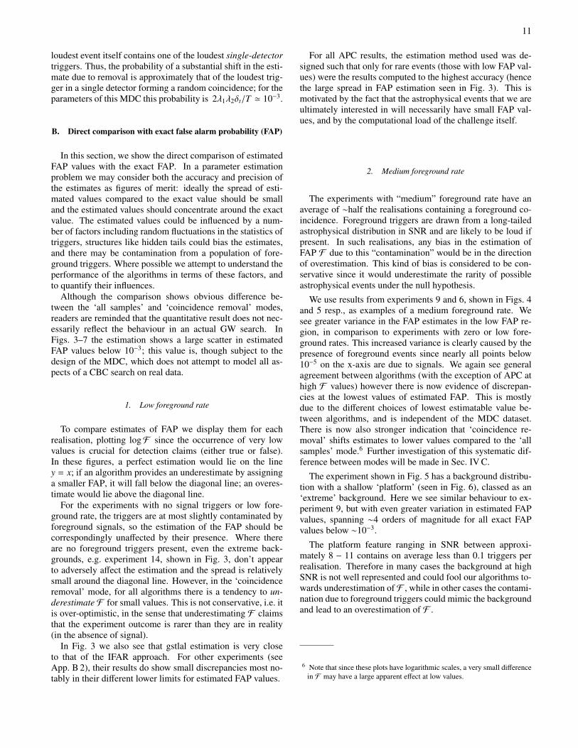
Although the comparison shows obvious difference be-tween the ‘all samples’ and ‘coincidence removal’ modes,readers are reminded that the quantitative result does not nec-essarily reflect the behaviour in an actual GW search. InFigs. 3–7 the estimation shows a large scatter in estimatedFAP values below 10−3; this value is, though subject to thedesign of the MDC, which does not attempt to model all as-pects of a CBC search on real data.
1. Low foreground rate
To compare estimates of FAP we display them for eachrealisation, plotting logF since the occurrence of very lowvalues is crucial for detection claims (either true or false).In these figures, a perfect estimation would lie on the liney = x; if an algorithm provides an underestimate by assigninga smaller FAP, it will fall below the diagonal line; an overes-timate would lie above the diagonal line.
For the experiments with no signal triggers or low fore-ground rate, the triggers are at most slightly contaminated byforeground signals, so the estimation of the FAP should becorrespondingly unaffected by their presence. Where thereare no foreground triggers present, even the extreme back-grounds, e.g. experiment 14, shown in Fig. 3, don’t appearto adversely affect the estimation and the spread is relativelysmall around the diagonal line. However, in the ‘coincidenceremoval’ mode, for all algorithms there is a tendency to un-derestimate F for small values. This is not conservative, i.e. itis over-optimistic, in the sense that underestimating F claimsthat the experiment outcome is rarer than they are in reality(in the absence of signal).
In Fig. 3 we also see that gstlal estimation is very closeto that of the IFAR approach. For other experiments (seeApp. B 2), their results do show small discrepancies most no-tably in their different lower limits for estimated FAP values.
For all APC results, the estimation method used was de-signed such that only for rare events (those with low FAP val-ues) were the results computed to the highest accuracy (hencethe large spread in FAP estimation seen in Fig. 3). This ismotivated by the fact that the astrophysical events that we areultimately interested in will necessarily have small FAP val-ues, and by the computational load of the challenge itself.
2. Medium foreground rate
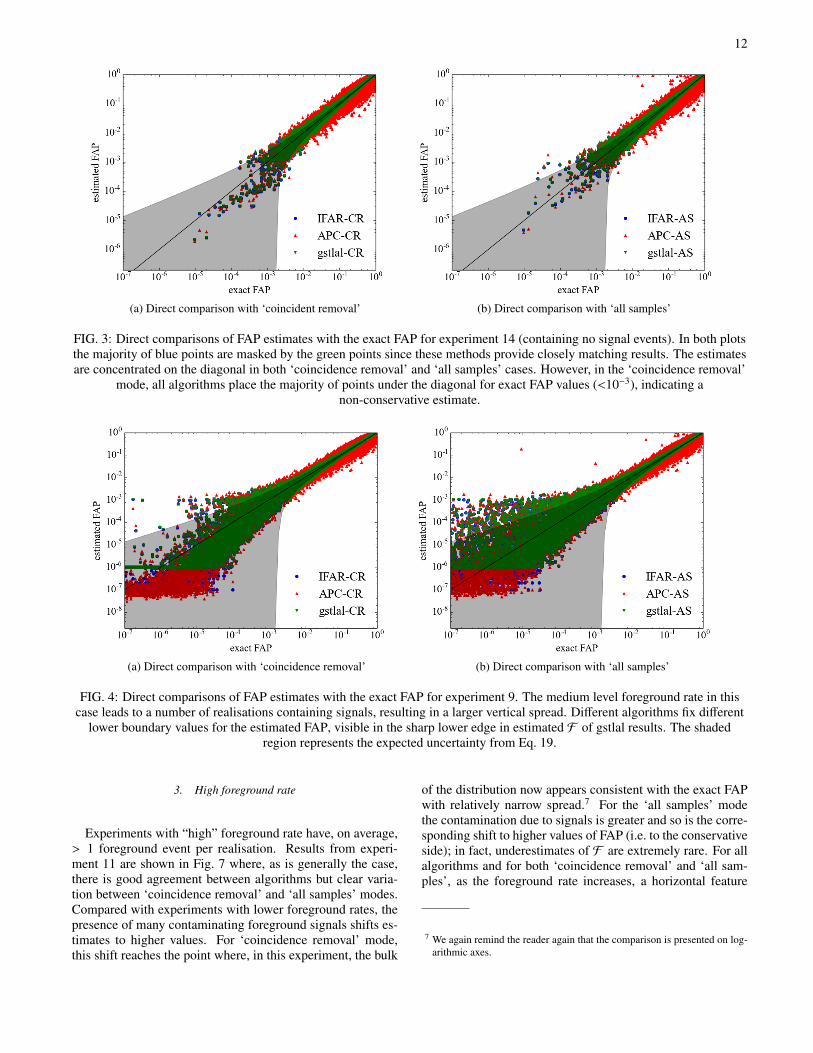
The experiments with “medium” foreground rate have anaverage of ∼half the realisations containing a foreground co-incidence. Foreground triggers are drawn from a long-tailedastrophysical distribution in SNR and are likely to be loud ifpresent. In such realisations, any bias in the estimation ofFAP F due to this “contamination” would be in the directionof overestimation. This kind of bias is considered to be con-servative since it would underestimate the rarity of possibleastrophysical events under the null hypothesis.
We use results from experiments 9 and 6, shown in Figs. 4and 5 resp., as examples of a medium foreground rate. Wesee greater variance in the FAP estimates in the low FAP re-gion, in comparison to experiments with zero or low fore-ground rates. This increased variance is clearly caused by thepresence of foreground events since nearly all points below10−5 on the x-axis are due to signals. We again see generalagreement between algorithms (with the exception of APC athigh F values) however there is now evidence of discrepan-cies at the lowest values of estimated FAP. This is mostlydue to the different choices of lowest estimatable value be-tween algorithms, and is independent of the MDC dataset.There is now also stronger indication that ‘coincidence re-moval’ shifts estimates to lower values compared to the ‘allsamples’ mode.6 Further investigation of this systematic dif-ference between modes will be made in Sec. IV C.
The experiment shown in Fig. 5 has a background distribu-tion with a shallow ‘platform’ (seen in Fig. 6), classed as an‘extreme’ background. Here we see similar behaviour to ex-periment 9, but with even greater variation in estimated FAPvalues, spanning ∼4 orders of magnitude for all exact FAPvalues below ∼10−3.
The platform feature ranging in SNR between approxi-mately 8 − 11 contains on average less than 0.1 triggers perrealisation. Therefore in many cases the background at highSNR is not well represented and could fool our algorithms to-wards underestimation of F , while in other cases the contami-nation due to foreground triggers could mimic the backgroundand lead to an overestimation of F .
6 Note that since these plots have logarithmic scales, a very small differencein F may have a large apparent effect at low values.
12
(a) Direct comparison with ‘coincident removal’ (b) Direct comparison with ‘all samples’
FIG. 3: Direct comparisons of FAP estimates with the exact FAP for experiment 14 (containing no signal events). In both plotsthe majority of blue points are masked by the green points since these methods provide closely matching results. The estimatesare concentrated on the diagonal in both ‘coincidence removal’ and ‘all samples’ cases. However, in the ‘coincidence removal’
mode, all algorithms place the majority of points under the diagonal for exact FAP values (<10−3), indicating anon-conservative estimate.
(a) Direct comparison with ‘coincidence removal’ (b) Direct comparison with ‘all samples’
FIG. 4: Direct comparisons of FAP estimates with the exact FAP for experiment 9. The medium level foreground rate in thiscase leads to a number of realisations containing signals, resulting in a larger vertical spread. Different algorithms fix different
lower boundary values for the estimated FAP, visible in the sharp lower edge in estimated F of gstlal results. The shadedregion represents the expected uncertainty from Eq. 19.
3. High foreground rate
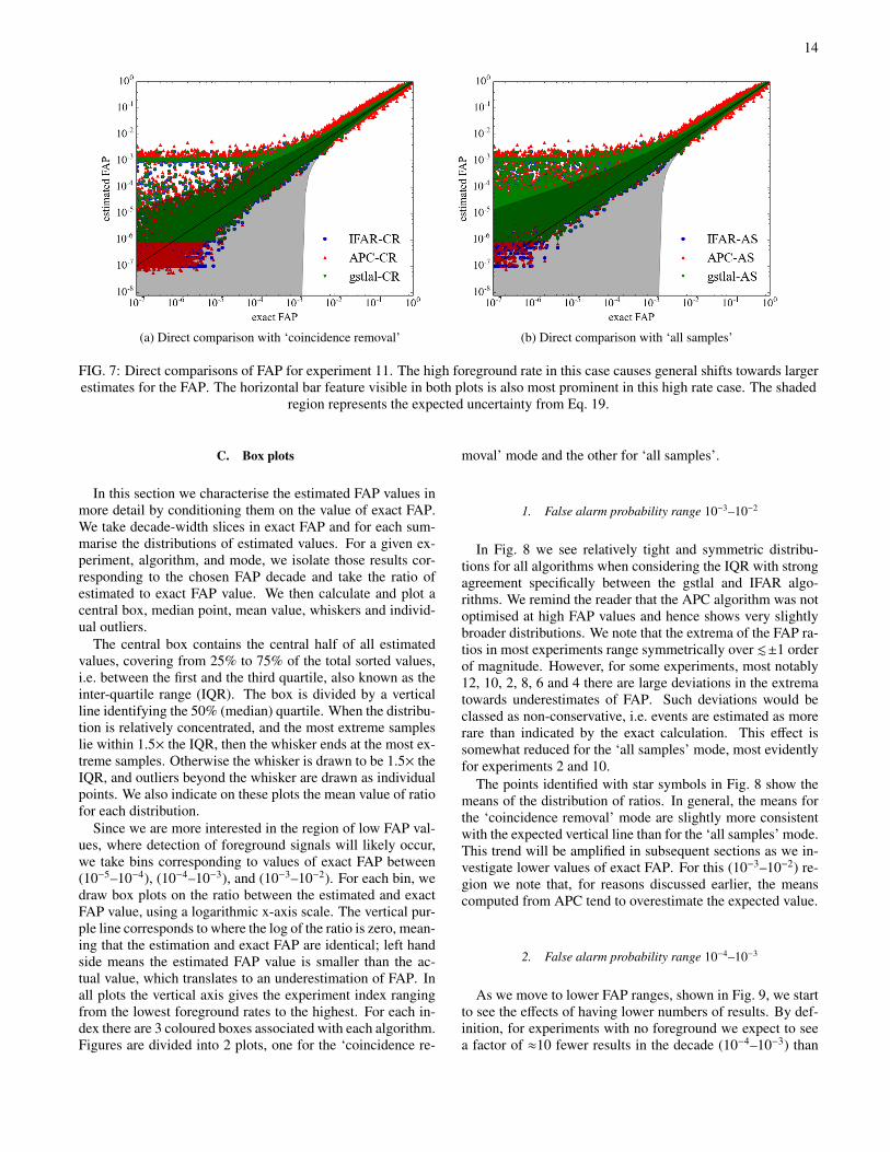
Experiments with “high” foreground rate have, on average,> 1 foreground event per realisation. Results from experi-ment 11 are shown in Fig. 7 where, as is generally the case,there is good agreement between algorithms but clear varia-tion between ‘coincidence removal’ and ‘all samples’ modes.Compared with experiments with lower foreground rates, thepresence of many contaminating foreground signals shifts es-timates to higher values. For ‘coincidence removal’ mode,this shift reaches the point where, in this experiment, the bulk
of the distribution now appears consistent with the exact FAPwith relatively narrow spread.7 For the ‘all samples’ modethe contamination due to signals is greater and so is the corre-sponding shift to higher values of FAP (i.e. to the conservativeside); in fact, underestimates of F are extremely rare. For allalgorithms and for both ‘coincidence removal’ and ‘all sam-ples’, as the foreground rate increases, a horizontal feature
7 We again remind the reader again that the comparison is presented on log-arithmic axes.

13
(a) Direct comparison with ‘coincidence removal’ (b) Direct comparison with ‘all samples’
FIG. 5: Direct comparisons of FAP for experiment 6. The presence of a platform feature in the tail of the distribution causes thespread in estimates values to be wider than for experiment 9. The shaded region represents the expected uncertainty from
Eq. 19.
FIG. 6: Reverse CDF of trigger SNRs for experiment 6. Thered and green curves represent the two individual detectors,
while the blue curve represents the astronomical signals. Theblack lines represent the combined distribution of both
background and foreground triggers.
appears in these comparison plots, which we discuss in thefollowing section.
4. Horizontal bar feature
In all high foreground rate scenarios, horizontal features ap-pear at ∼10−3 in estimated FAP, which are also marginallyvisible in medium rate experiments. The process of FAP esti-mation for the loudest coincident event is based on collectingthe fraction of all possible unphysical coincidences which arelouder. The estimation will be strongly biased when there ex-ists a foreground trigger in one detector that is extremely loudand either not found in coincidence in zero-lag, or coincidentwith a trigger with very low SNR. In such cases it is highly
likely that when performing background estimation it wouldresult in background coincidences which are louder than theloudest zero-lag event (the details of this process are specificto each algorithm). Assuming a method that makes use of allpossible unphysical trigger combinations between detectors,this corresponds to ∼104 louder background coincidences outof a possible ∼108 in total. Considering an expected ∼10 zero-lag coincidences this gives an estimated FAP of these asym-metric events as ∼10−3.
In experiment 11 (Fig. 7), there are ∼ 650 such realisations.For ∼ 500 of them, the cause is a single astrophysical signalappearing as an extremely loud trigger in one detector, whilefor the other detector the combination of antenna pattern andnon-central χ2 random fluctuations results in a sub-thresholdSNR and is hence not recorded as a trigger. The remaining∼ 150 events also have very loud SNRs in one detector, but inthese cases the counterpart in the second detector appears onlyas a relatively weak trigger. When foreground events appearwith asymmetrical SNRs between the two detectors, remov-ing coincident triggers from the background estimate couldmitigate overestimation occurring in such cases; while for the∼500 realisations that contain a single loud foreground triggerwhich does not form a coincidence, overestimation will occurregardless of the method used.
5. Uncertainty estimate
Throughout figure 3 - 7, a shaded region was plotted whichrepresents the uncertainty predicted from Eq. 19. In thederivation of Eq. 19 several simplifying assumptions wereused, thus some discrepancy between the theoretical expec-tation and the actual spread is not surprising. However, thisexpression does capture the order of magnitude of the uncer-tainty, so as a “rule of thumb” it serves as a guide in the esti-mation of uncertainty for the FAP.
14
(a) Direct comparison with ‘coincidence removal’ (b) Direct comparison with ‘all samples’
FIG. 7: Direct comparisons of FAP for experiment 11. The high foreground rate in this case causes general shifts towards largerestimates for the FAP. The horizontal bar feature visible in both plots is also most prominent in this high rate case. The shaded
region represents the expected uncertainty from Eq. 19.
C. Box plots
In this section we characterise the estimated FAP values inmore detail by conditioning them on the value of exact FAP.We take decade-width slices in exact FAP and for each sum-marise the distributions of estimated values. For a given ex-periment, algorithm, and mode, we isolate those results cor-responding to the chosen FAP decade and take the ratio ofestimated to exact FAP value. We then calculate and plot acentral box, median point, mean value, whiskers and individ-ual outliers.
The central box contains the central half of all estimatedvalues, covering from 25% to 75% of the total sorted values,i.e. between the first and the third quartile, also known as theinter-quartile range (IQR). The box is divided by a verticalline identifying the 50% (median) quartile. When the distribu-tion is relatively concentrated, and the most extreme sampleslie within 1.5× the IQR, then the whisker ends at the most ex-treme samples. Otherwise the whisker is drawn to be 1.5× theIQR, and outliers beyond the whisker are drawn as individualpoints. We also indicate on these plots the mean value of ratiofor each distribution.
Since we are more interested in the region of low FAP val-ues, where detection of foreground signals will likely occur,we take bins corresponding to values of exact FAP between(10−5–10−4), (10−4–10−3), and (10−3–10−2). For each bin, wedraw box plots on the ratio between the estimated and exactFAP value, using a logarithmic x-axis scale. The vertical pur-ple line corresponds to where the log of the ratio is zero, mean-ing that the estimation and exact FAP are identical; left handside means the estimated FAP value is smaller than the ac-tual value, which translates to an underestimation of FAP. Inall plots the vertical axis gives the experiment index rangingfrom the lowest foreground rates to the highest. For each in-dex there are 3 coloured boxes associated with each algorithm.Figures are divided into 2 plots, one for the ‘coincidence re-
moval’ mode and the other for ‘all samples’.
1. False alarm probability range 10−3–10−2
In Fig. 8 we see relatively tight and symmetric distribu-tions for all algorithms when considering the IQR with strongagreement specifically between the gstlal and IFAR algo-rithms. We remind the reader that the APC algorithm was notoptimised at high FAP values and hence shows very slightlybroader distributions. We note that the extrema of the FAP ra-tios in most experiments range symmetrically over .±1 orderof magnitude. However, for some experiments, most notably12, 10, 2, 8, 6 and 4 there are large deviations in the extrematowards underestimates of FAP. Such deviations would beclassed as non-conservative, i.e. events are estimated as morerare than indicated by the exact calculation. This effect issomewhat reduced for the ‘all samples’ mode, most evidentlyfor experiments 2 and 10.
The points identified with star symbols in Fig. 8 show themeans of the distribution of ratios. In general, the means forthe ‘coincidence removal’ mode are slightly more consistentwith the expected vertical line than for the ‘all samples’ mode.This trend will be amplified in subsequent sections as we in-vestigate lower values of exact FAP. For this (10−3–10−2) re-gion we note that, for reasons discussed earlier, the meanscomputed from APC tend to overestimate the expected value.
2. False alarm probability range 10−4–10−3
As we move to lower FAP ranges, shown in Fig. 9, we startto see the effects of having lower numbers of results. By def-inition, for experiments with no foreground we expect to seea factor of ≈10 fewer results in the decade (10−4–10−3) than

15
(a) Box plots based on ‘coincidence removal’.
(b) Box plots based on ‘all samples’
FIG. 8: Box plots of the ratio of estimated to exact FAPvalue, for exact FAPs between 10−3 and 10−2. The shaded
region represents the expected uncertainty from Eq. 19.
in the decade (10−3–10−2), implying larger statistical fluctu-ations due to the reduced number of samples. We also seeintrinsically broader distributions, as the estimation methodsthemselves are constrained by the infrequency of loud, low-FAP events. As seen in previous figures of merit, results differonly slightly between algorithms with the largest differencescoming from the issue of inclusion or removal of coincidenttriggers.
Overall, we see ranges in the extrema spanning ±1 order ofmagnitude for both ‘coincidence removal’ and ‘all samples’modes. However, for experiments 10, 2, 6, and 8 the lowerextrema extend to ∼ 4 order of magnitude below the expectedratio for the ‘coincidence removal’ mode. This behaviour ismitigated for the ‘all samples’ mode: note that for experiment10 the extrema are reduced to be consistent with the major-ity of other experiments. In general it is clear that the IQRsfor the ‘coincidence removal’ mode are broader in logarithmicspace than for ‘all samples’. This increase in width is always
(a) Box plots based on ‘coincidence removal’
(b) Box plots based on ‘all samples’
FIG. 9: Box plots of the ratio of estimated to exact FAPvalue, for exact FAPs between 10−4 and 10−3. The shaded
region represents the expected uncertainty from Eq. 19.
to lower values of the ratio, implying underestimation of theFAP. This trend is also exemplified by the locations of themedian values: for the ‘coincidence removal’ mode, low fore-ground rates yield medians skewed to lower values by factorsof ∼2–200. For the 3 high foreground rate experiments theIQRs and corresponding medians appear consistent with theexact FAP. For the ‘all samples’ mode the IQRs and mediansare relatively symmetric about the exact FAP and the IQRs arein all cases narrower than for the ‘coincidence removal’ mode.
In this FAP range the difference in distribution means be-tween the ‘coincidence removal’ and ‘all samples’ modes be-comes more obvious. The removal mode results consistentlyreturn mean estimates well within factors of 2 for all no, lowand medium foreground rates. For high foreground rates theyconsistently overestimate the means by up to a factor of ∼ 3.For the ‘all samples’ mode there is a clear overestimate of theratio (implying a conservative overestimate of the FAP) forall experiments irrespective of foreground rate or background
16
complexity. This overestimate is in general a factor of ∼2.Note though that the estimates from both modes for the threehigh foreground rate experiments are very similar in their dis-tributions and means.
3. False alarm probability range 10−5–10−4
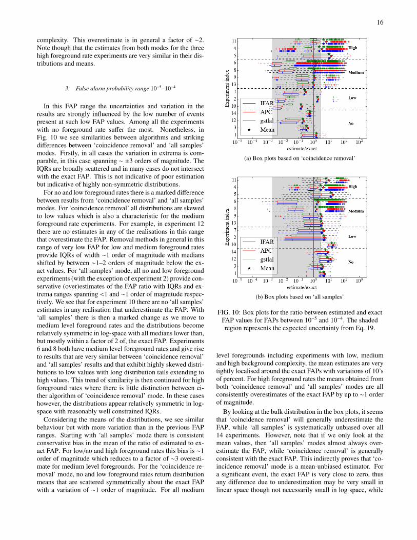
In this FAP range the uncertainties and variation in theresults are strongly influenced by the low number of eventspresent at such low FAP values. Among all the experimentswith no foreground rate suffer the most. Nonetheless, inFig. 10 we see similarities between algorithms and strikingdifferences between ‘coincidence removal’ and ‘all samples’modes. Firstly, in all cases the variation in extrema is com-parable, in this case spanning ∼ ±3 orders of magnitude. TheIQRs are broadly scattered and in many cases do not intersectwith the exact FAP. This is not indicative of poor estimationbut indicative of highly non-symmetric distributions.
For no and low foreground rates there is a marked differencebetween results from ‘coincidence removal’ and ‘all samples’modes. For ‘coincidence removal’ all distributions are skewedto low values which is also a characteristic for the mediumforeground rate experiments. For example, in experiment 12there are no estimates in any of the realisations in this rangethat overestimate the FAP. Removal methods in general in thisrange of very low FAP for low and medium foreground ratesprovide IQRs of width ∼1 order of magnitude with mediansshifted by between ∼1–2 orders of magnitude below the ex-act values. For ‘all samples’ mode, all no and low foregroundexperiments (with the exception of experiment 2) provide con-servative (over)estimates of the FAP ratio with IQRs and ex-trema ranges spanning <1 and ∼1 order of magnitude respec-tively. We see that for experiment 10 there are no ‘all samples’estimates in any realisation that underestimate the FAP. With‘all samples’ there is then a marked change as we move tomedium level foreground rates and the distributions becomerelatively symmetric in log-space with all medians lower than,but mostly within a factor of 2 of, the exact FAP. Experiments6 and 8 both have medium level foreground rates and give riseto results that are very similar between ‘coincidence removal’and ‘all samples’ results and that exhibit highly skewed distri-butions to low values with long distribution tails extending tohigh values. This trend of similarity is then continued for highforeground rates where there is little distinction between ei-ther algorithm of ‘coincidence removal’ mode. In these caseshowever, the distributions appear relatively symmetric in log-space with reasonably well constrained IQRs.
Considering the means of the distributions, we see similarbehaviour but with more variation than in the previous FAPranges. Starting with ‘all samples’ mode there is consistentconservative bias in the mean of the ratio of estimated to ex-act FAP. For low/no and high foreground rates this bias is ∼1order of magnitude which reduces to a factor of ∼3 overesti-mate for medium level foregrounds. For the ‘coincidence re-moval’ mode, no and low foreground rates return distributionmeans that are scattered symmetrically about the exact FAPwith a variation of ∼1 order of magnitude. For all medium
(a) Box plots based on ‘coincidence removal’
(b) Box plots based on ‘all samples’
FIG. 10: Box plots for the ratio between estimated and exactFAP values for FAPs between 10−5 and 10−4. The shadedregion represents the expected uncertainty from Eq. 19.
level foregrounds including experiments with low, mediumand high background complexity, the mean estimates are verytightly localised around the exact FAPs with variations of 10’sof percent. For high foreground rates the means obtained fromboth ‘coincidence removal’ and ‘all samples’ modes are allconsistently overestimates of the exact FAP by up to ∼1 orderof magnitude.
By looking at the bulk distribution in the box plots, it seemsthat ‘coincidence removal’ will generally underestimate theFAP, while ‘all samples’ is systematically unbiased over all14 experiments. However, note that if we only look at themean values, then ‘all samples’ modes almost always over-estimate the FAP, while ‘coincidence removal’ is generallyconsistent with the exact FAP. This indirectly proves that ‘co-incidence removal’ mode is a mean-unbiased estimator. Fora significant event, the exact FAP is very close to zero, thusany difference due to underestimation may be very small inlinear space though not necessarily small in log space, while

17
FIG. 11: ROC plot for experiment 2. The error bars in bothhorizontal and vertical directions are calculated with a
binomial likelihood under a 68% credible interval. Solidlines correspond to ‘all samples’, while dashed lines
corresponds to ‘coincidence removal’. The dotted linerepresents the expected performance of random guess, no
rational analysis would perform worse than it.
overestimation could bias the value with a large relative devi-ation. When the FAP is very small, the estimation uncertainty(variance) is large relative to the exact value; then, since esti-mated values are bounded below by zero, in order to achievea mean-unbiased estimate a large majority of estimated valuesare necessarily below the exact value, i.e. underestimates. Inother words, the distribution is highly skewed.
D. ROC analyses
The FAP value is a measure of the rarity of observed events,but in this section we treat the estimated FAP as a test statis-tic. This allows us to use ROC plots to compare the ability todistinguish signal from noise for each method. In practice thisinvolves taking one of our experiments containing 105 reali-sations and, as a function of a variable threshold on our teststatistic (the FAP), computing the following. The false posi-tive rate (FPR) is the fraction of loudest events due to back-ground that had estimated FAP values below the threshold.The true positive rate (TPR) is computed as the fraction ofloudest events due to the foreground that had estimated FAPsbelow the threshold. For each choice of threshold a point canbe placed in the FPR-TPR plane creating an ROC curve for agiven test-statistic. Better performing statistics have a higherTPR at a given FPR. A perfect method would recover 100% ofthe signals while incurring no false alarms, corresponding toa ROC curve that passes through the upper left corner. A ran-dom classifier assigning uniformly distributed random num-bers to the FAP would lead to identical FPR and TPR, yieldinga diagonal ROC curve.
Error regions for the FPR and TPR are computed using abinomial likelihood function. In general, as can be seen in our
ROC plots, as the foreground rate goes up, the more events areavailable to compute the TPR, reducing the vertical uncertain-ties. Conversely, the more background events are available,the smaller the horizontal uncertainties.
In the following subsections we focus on the experimentswhere there are clear discrepancies, leaving cases where thereis agreement between methods to Appendix B 3. We stressthat ROC curves allow us to assess the ability of a test-statisticto distinguish between realisations where the loudest eventis foreground vs. background; however they make no directstatement on the accuracy or precision of FAP estimation.
1. Low foreground rate
There are 3 experiments, 2, 7 and 10, that have low fore-ground rates. The ROC curve for experiment 2 in Fig. 11 ex-hibits a number of interesting features. Firstly, there is generalagreement between algorithms; deviations are only visible be-tween ‘coincidence removal’ and ‘all samples’ modes of op-eration. At a FPR of ∼10−3 and below, the ‘all samples’ modeappear to achieve higher TPRs, when accounting for their re-spective uncertainties, by ∼ 10%. This indicates that in thislow-rate case, where ≈ 1 in 1000 loudest events were actualforeground signals, the ‘all samples’ mode is more efficient atdetecting signals at low FPRs. We can identify all experimentsthat show such deviations, and all have tail features or obviousasymmetry between the two detectors’ background distribu-tions, combined with a low to medium foreground rate.
2. Medium foreground rate
Experiments 6, 8, 9 and 13 contain medium foregroundrates and collectively show two types of behaviour. Ex-periments 9 and 13 show general agreement between algo-rithms and ‘coincidence removal’ and ‘all samples’ modes(see Figs. 37 and 40). Experiments 6 and 8 show similar de-viations to those seen in the p–p plots in Section IV A. Thissimilarity is not surprising since the vertical axes of the p-pplots are identical to horizontal axes of the ROC plots, withthe distinction that they are computed on background-onlyand background-foreground experiments respectively.
Here we focus on Experiment 8 shown in Fig. 12 whichcontained realistic but slightly different background distribu-tions in each detector. As seen in the low-foreground examplethere is good agreement between algorithms but differencesbetween ‘coincidence removal’ and ‘all samples’ modes. Inthis case, due to the increased number of foreground events,this difference is more clearly visible and the disscrepan-cies are inconsistent with the estimated uncertainties. Sofor medium foreground rates we conclude that as a detectionstatistic, the ‘all samples’ mode obtains higher TPRs at fixedFPR for low values of FAP. We remind the reader that de-tection claims will be made at low FAP values, although theabsolute values appearing in our MDC may not be represen-tative of those obtained by algorithms in a realistic analysis.
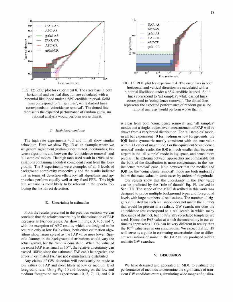
18
FIG. 12: ROC plot for experiment 8. The error bars in bothhorizontal and vertical direction are calculated with a
binomial likelihood under a 68% credible interval. Solidlines correspond to ‘all samples’, while dashed lines
corresponds to ‘coincidence removal’. The dotted linerepresents the expected performance of random guess, no
rational analysis would perform worse than it.
3. High foreground rate
The high rate experiments 4, 5 and 11 all show similarbehaviour. Here we show Fig. 13 as an example where wesee general agreement (within our estimated uncertainties) be-tween algorithms and between the ‘coincidence removal’ and‘all samples’ modes. The high rates used result in >90% of re-alisations containing a loudest coincident event from the fore-ground. The 3 experiments were examples of all 3 levels ofbackground complexity respectively and the results indicatethat in terms of detection efficiency, all algorithms and ap-proaches perform equally well at any fixed FPR. This highrate scenario is most likely to be relevant in the epochs fol-lowing the first direct detection.
E. Uncertainty in estimation
From the results presented in the previous sections we canconclude that the relative uncertainty in the estimation of FAPincreases as FAP decreases. As shown in Figs. 3, 4, 5, and 7,with the exception of APC results, which are designed to beaccurate only at low FAP values, both other estimation algo-rithms show larger spread as the FAP value goes lower. Spe-cific features in the background distributions would vary theactual spread, but the trend is consistent. When the value ofthe exact FAP is as small as 10−4, the relative uncertainty canexceed 100%; since the estimated FAP can’t be negative, theerrors in estimated FAP are not symmetrically distributed.
Any claims of GW detection will necessarily be made atlow values of FAP and most likely at low or medium levelforeground rate. Using Fig. 10 and focusing on the low andmedium foreground rate experiments 10, 2, 7, 13, and 9 it
FIG. 13: ROC plot for experiment 4. The error bars in bothhorizontal and vertical direction are calculated with a
binomial likelihood under a 68% credible interval. Solidlines correspond to ‘all samples’, while dashed linescorrespond to ‘coincidence removal’. The dotted line
represents the expected performance of random guess, norational analysis would perform worse than it.
is clear from both ‘coincidence removal’ and ‘all samples’modes that a single loudest event measurement of FAP will bedrawn from a very broad distribution. For ‘all samples’ mode,in all but experiment 10 for medium or low foregrounds, theIQR looks symmetric mostly consistent with the true valuewithin ±1 order of magnitude. For the equivalent ‘coincidenceremoval’ mode results, the IQR is much smaller than its coun-terpart in the ‘all sample’ mode in log-space, and hence moreprecise. The extrema between approaches are comparable butthe bulk of the distribution is more concentrated in the ‘co-incidence removal’ case. Note however that the median andIQR for the ‘coincidence removal’ mode are both uniformlybelow the exact value, in some cases by orders of magnitude.
Our results show that the uncertainty in the FAP valuecan be predicted by the “rule of thumb” Eq. 19, derived inSec. II D. The scope of the MDC described in this work wasdesigned to probe multiple background types and foregroundlevels with large numbers of realisations. The number of trig-gers simulated for each realisation does not match the numberthat would be present in a realistic GW search; nor does thecoincidence test correspond to a real search in which manythousands of distinct, but nontrivially correlated templates areused. Hence, the FAP value at which the uncertainty in our es-timates approaches 100% can be very different in reality thanthe 10−3 value seen in our simulations. We expect that Eq. 19will serve as a guide in estimating uncertainties due to differ-ent realisations of noise in the FAP values produced withinrealistic GW searches.
V. DISCUSSION
We have designed and generated an MDC to evaluate theperformance of methods to determine the significance of tran-sient GW candidate events, simulating wide ranges of qualita-
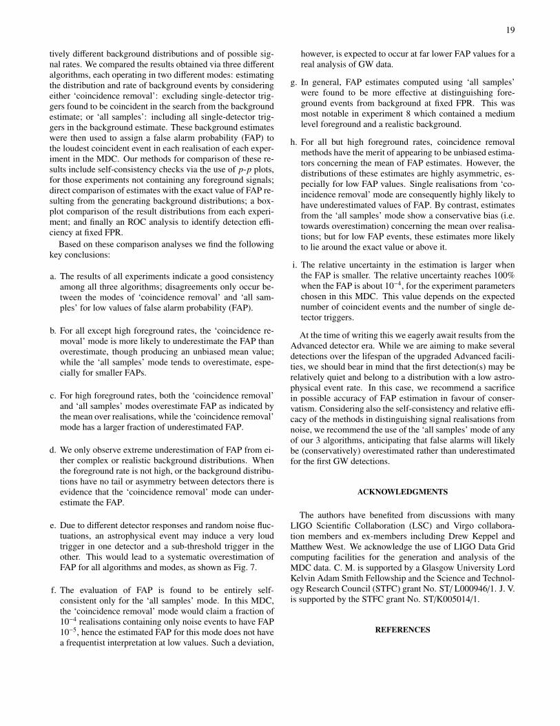
19
tively different background distributions and of possible sig-nal rates. We compared the results obtained via three differentalgorithms, each operating in two different modes: estimatingthe distribution and rate of background events by consideringeither ‘coincidence removal’: excluding single-detector trig-gers found to be coincident in the search from the backgroundestimate; or ‘all samples’: including all single-detector trig-gers in the background estimate. These background estimateswere then used to assign a false alarm probability (FAP) tothe loudest coincident event in each realisation of each exper-iment in the MDC. Our methods for comparison of these re-sults include self-consistency checks via the use of p-p plots,for those experiments not containing any foreground signals;direct comparison of estimates with the exact value of FAP re-sulting from the generating background distributions; a box-plot comparison of the result distributions from each experi-ment; and finally an ROC analysis to identify detection effi-ciency at fixed FPR.
Based on these comparison analyses we find the followingkey conclusions:
a. The results of all experiments indicate a good consistencyamong all three algorithms; disagreements only occur be-tween the modes of ‘coincidence removal’ and ‘all sam-ples’ for low values of false alarm probability (FAP).
b. For all except high foreground rates, the ‘coincidence re-moval’ mode is more likely to underestimate the FAP thanoverestimate, though producing an unbiased mean value;while the ‘all samples’ mode tends to overestimate, espe-cially for smaller FAPs.
c. For high foreground rates, both the ‘coincidence removal’and ‘all samples’ modes overestimate FAP as indicated bythe mean over realisations, while the ‘coincidence removal’mode has a larger fraction of underestimated FAP.
d. We only observe extreme underestimation of FAP from ei-ther complex or realistic background distributions. Whenthe foreground rate is not high, or the background distribu-tions have no tail or asymmetry between detectors there isevidence that the ‘coincidence removal’ mode can under-estimate the FAP.
e. Due to different detector responses and random noise fluc-tuations, an astrophysical event may induce a very loudtrigger in one detector and a sub-threshold trigger in theother. This would lead to a systematic overestimation ofFAP for all algorithms and modes, as shown as Fig. 7.
f. The evaluation of FAP is found to be entirely self-consistent only for the ‘all samples’ mode. In this MDC,the ‘coincidence removal’ mode would claim a fraction of10−4 realisations containing only noise events to have FAP10−5, hence the estimated FAP for this mode does not havea frequentist interpretation at low values. Such a deviation,
however, is expected to occur at far lower FAP values for areal analysis of GW data.
g. In general, FAP estimates computed using ‘all samples’were found to be more effective at distinguishing fore-ground events from background at fixed FPR. This wasmost notable in experiment 8 which contained a mediumlevel foreground and a realistic background.
h. For all but high foreground rates, coincidence removalmethods have the merit of appearing to be unbiased estima-tors concerning the mean of FAP estimates. However, thedistributions of these estimates are highly asymmetric, es-pecially for low FAP values. Single realisations from ‘co-incidence removal’ mode are consequently highly likely tohave underestimated values of FAP. By contrast, estimatesfrom the ‘all samples’ mode show a conservative bias (i.e.towards overestimation) concerning the mean over realisa-tions; but for low FAP events, these estimates more likelyto lie around the exact value or above it.
i. The relative uncertainty in the estimation is larger whenthe FAP is smaller. The relative uncertainty reaches 100%when the FAP is about 10−4, for the experiment parameterschosen in this MDC. This value depends on the expectednumber of coincident events and the number of single de-tector triggers.
At the time of writing this we eagerly await results from theAdvanced detector era. While we are aiming to make severaldetections over the lifespan of the upgraded Advanced facili-ties, we should bear in mind that the first detection(s) may berelatively quiet and belong to a distribution with a low astro-physical event rate. In this case, we recommend a sacrificein possible accuracy of FAP estimation in favour of conser-vatism. Considering also the self-consistency and relative effi-cacy of the methods in distinguishing signal realisations fromnoise, we recommend the use of the ‘all samples’ mode of anyof our 3 algorithms, anticipating that false alarms will likelybe (conservatively) overestimated rather than underestimatedfor the first GW detections.
ACKNOWLEDGMENTS
The authors have benefited from discussions with manyLIGO Scientific Collaboration (LSC) and Virgo collabora-tion members and ex-members including Drew Keppel andMatthew West. We acknowledge the use of LIGO Data Gridcomputing facilities for the generation and analysis of theMDC data. C. M. is supported by a Glasgow University LordKelvin Adam Smith Fellowship and the Science and Technol-ogy Research Council (STFC) grant No. ST/ L000946/1. J. V.is supported by the STFC grant No. ST/K005014/1.
REFERENCES
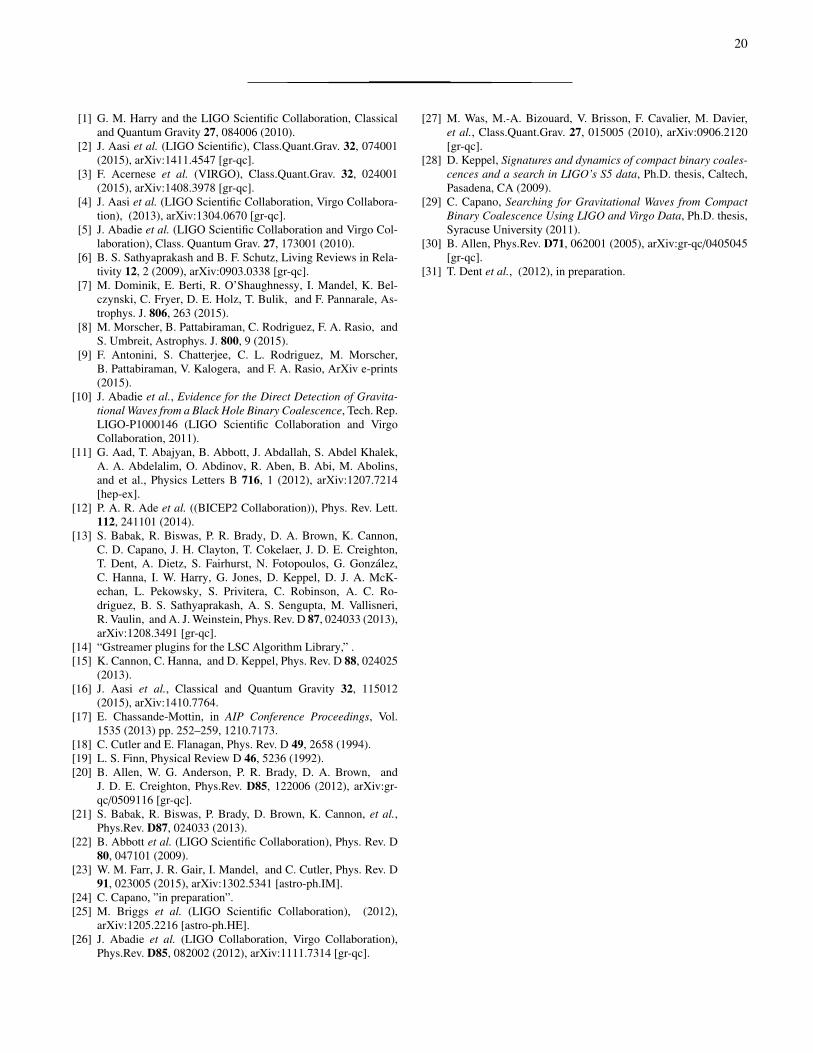
20
[1] G. M. Harry and the LIGO Scientific Collaboration, Classicaland Quantum Gravity 27, 084006 (2010).
[2] J. Aasi et al. (LIGO Scientific), Class.Quant.Grav. 32, 074001(2015), arXiv:1411.4547 [gr-qc].
[3] F. Acernese et al. (VIRGO), Class.Quant.Grav. 32, 024001(2015), arXiv:1408.3978 [gr-qc].
[4] J. Aasi et al. (LIGO Scientific Collaboration, Virgo Collabora-tion), (2013), arXiv:1304.0670 [gr-qc].
[5] J. Abadie et al. (LIGO Scientific Collaboration and Virgo Col-laboration), Class. Quantum Grav. 27, 173001 (2010).
[6] B. S. Sathyaprakash and B. F. Schutz, Living Reviews in Rela-tivity 12, 2 (2009), arXiv:0903.0338 [gr-qc].
[7] M. Dominik, E. Berti, R. O’Shaughnessy, I. Mandel, K. Bel-czynski, C. Fryer, D. E. Holz, T. Bulik, and F. Pannarale, As-trophys. J. 806, 263 (2015).
[8] M. Morscher, B. Pattabiraman, C. Rodriguez, F. A. Rasio, andS. Umbreit, Astrophys. J. 800, 9 (2015).
[9] F. Antonini, S. Chatterjee, C. L. Rodriguez, M. Morscher,B. Pattabiraman, V. Kalogera, and F. A. Rasio, ArXiv e-prints(2015).
[10] J. Abadie et al., Evidence for the Direct Detection of Gravita-tional Waves from a Black Hole Binary Coalescence, Tech. Rep.LIGO-P1000146 (LIGO Scientific Collaboration and VirgoCollaboration, 2011).
[11] G. Aad, T. Abajyan, B. Abbott, J. Abdallah, S. Abdel Khalek,A. A. Abdelalim, O. Abdinov, R. Aben, B. Abi, M. Abolins,and et al., Physics Letters B 716, 1 (2012), arXiv:1207.7214[hep-ex].
[12] P. A. R. Ade et al. ((BICEP2 Collaboration)), Phys. Rev. Lett.112, 241101 (2014).
[13] S. Babak, R. Biswas, P. R. Brady, D. A. Brown, K. Cannon,C. D. Capano, J. H. Clayton, T. Cokelaer, J. D. E. Creighton,T. Dent, A. Dietz, S. Fairhurst, N. Fotopoulos, G. Gonzalez,C. Hanna, I. W. Harry, G. Jones, D. Keppel, D. J. A. McK-echan, L. Pekowsky, S. Privitera, C. Robinson, A. C. Ro-driguez, B. S. Sathyaprakash, A. S. Sengupta, M. Vallisneri,R. Vaulin, and A. J. Weinstein, Phys. Rev. D 87, 024033 (2013),arXiv:1208.3491 [gr-qc].
[14] “Gstreamer plugins for the LSC Algorithm Library,” .[15] K. Cannon, C. Hanna, and D. Keppel, Phys. Rev. D 88, 024025
(2013).[16] J. Aasi et al., Classical and Quantum Gravity 32, 115012
(2015), arXiv:1410.7764.[17] E. Chassande-Mottin, in AIP Conference Proceedings, Vol.
1535 (2013) pp. 252–259, 1210.7173.[18] C. Cutler and E. Flanagan, Phys. Rev. D 49, 2658 (1994).[19] L. S. Finn, Physical Review D 46, 5236 (1992).[20] B. Allen, W. G. Anderson, P. R. Brady, D. A. Brown, and
J. D. E. Creighton, Phys.Rev. D85, 122006 (2012), arXiv:gr-qc/0509116 [gr-qc].
[21] S. Babak, R. Biswas, P. Brady, D. Brown, K. Cannon, et al.,Phys.Rev. D87, 024033 (2013).
[22] B. Abbott et al. (LIGO Scientific Collaboration), Phys. Rev. D80, 047101 (2009).
[23] W. M. Farr, J. R. Gair, I. Mandel, and C. Cutler, Phys. Rev. D91, 023005 (2015), arXiv:1302.5341 [astro-ph.IM].
[24] C. Capano, ”in preparation”.[25] M. Briggs et al. (LIGO Scientific Collaboration), (2012),
arXiv:1205.2216 [astro-ph.HE].[26] J. Abadie et al. (LIGO Collaboration, Virgo Collaboration),
Phys.Rev. D85, 082002 (2012), arXiv:1111.7314 [gr-qc].
[27] M. Was, M.-A. Bizouard, V. Brisson, F. Cavalier, M. Davier,et al., Class.Quant.Grav. 27, 015005 (2010), arXiv:0906.2120[gr-qc].
[28] D. Keppel, Signatures and dynamics of compact binary coales-cences and a search in LIGO’s S5 data, Ph.D. thesis, Caltech,Pasadena, CA (2009).
[29] C. Capano, Searching for Gravitational Waves from CompactBinary Coalescence Using LIGO and Virgo Data, Ph.D. thesis,Syracuse University (2011).
[30] B. Allen, Phys.Rev. D71, 062001 (2005), arXiv:gr-qc/0405045[gr-qc].
[31] T. Dent et al., (2012), in preparation.
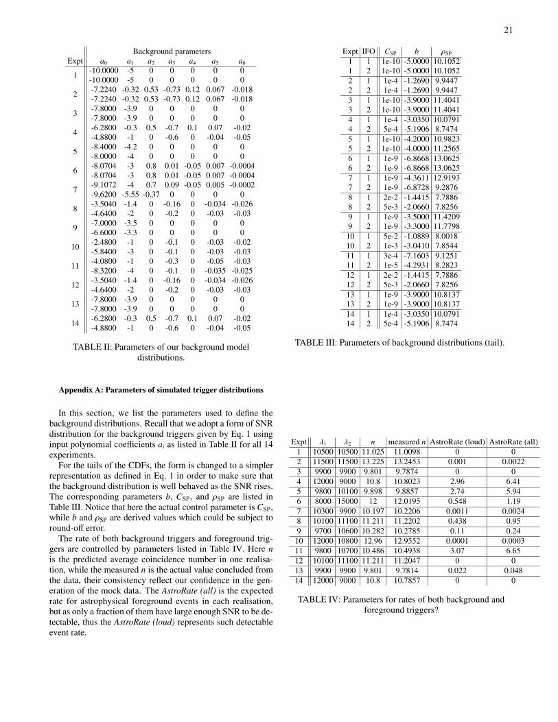
21
Background parametersExpt a0 a1 a2 a3 a4 a5 a6
1 -10.0000 -5 0 0 0 0 0-10.0000 -5 0 0 0 0 0
2 -7.2240 -0.32 0.53 -0.73 0.12 0.067 -0.018-7.2240 -0.32 0.53 -0.73 0.12 0.067 -0.018
3 -7.8000 -3.9 0 0 0 0 0-7.8000 -3.9 0 0 0 0 0
4 -6.2800 -0.3 0.5 -0.7 0.1 0.07 -0.02-4.8800 -1 0 -0.6 0 -0.04 -0.05
5 -8.4000 -4.2 0 0 0 0 0-8.0000 -4 0 0 0 0 0
6 -8.0704 -3 0.8 0.01 -0.05 0.007 -0.0004-8.0704 -3 0.8 0.01 -0.05 0.007 -0.0004
7 -9.1072 -4 0.7 0.09 -0.05 0.005 -0.0002-9.6200 -5.55 -0.37 0 0 0 0
8 -3.5040 -1.4 0 -0.16 0 -0.034 -0.026-4.6400 -2 0 -0.2 0 -0.03 -0.03
9 -7.0000 -3.5 0 0 0 0 0-6.6000 -3.3 0 0 0 0 0
10 -2.4800 -1 0 -0.1 0 -0.03 -0.02-5.8400 -3 0 -0.1 0 -0.03 -0.03
11 -4.0800 -1 0 -0.3 0 -0.05 -0.03-8.3200 -4 0 -0.1 0 -0.035 -0.025
12 -3.5040 -1.4 0 -0.16 0 -0.034 -0.026-4.6400 -2 0 -0.2 0 -0.03 -0.03
13 -7.8000 -3.9 0 0 0 0 0-7.8000 -3.9 0 0 0 0 0
14 -6.2800 -0.3 0.5 -0.7 0.1 0.07 -0.02-4.8800 -1 0 -0.6 0 -0.04 -0.05
TABLE II: Parameters of our background modeldistributions.
Appendix A: Parameters of simulated trigger distributions
In this section, we list the parameters used to define thebackground distributions. Recall that we adopt a form of SNRdistribution for the background triggers given by Eq. 1 usinginput polynomial coefficients ai as listed in Table II for all 14experiments.
For the tails of the CDFs, the form is changed to a simplerrepresentation as defined in Eq. 1 in order to make sure thatthe background distribution is well behaved as the SNR rises.The corresponding parameters b, CSP, and ρSP are listed inTable III. Notice that here the actual control parameter is CSP,while b and ρSP are derived values which could be subject toround-off error.
The rate of both background triggers and foreground trig-gers are controlled by parameters listed in Table IV. Here nis the predicted average coincidence number in one realisa-tion, while the measured n is the actual value concluded fromthe data, their consistency reflect our confidence in the gen-eration of the mock data. The AstroRate (all) is the expectedrate for astrophysical foreground events in each realisation,but as only a fraction of them have large enough SNR to be de-tectable, thus the AstroRate (loud) represents such detectableevent rate.
Expt IFO CSP b ρSP
1 1 1e-10 -5.0000 10.10521 2 1e-10 -5.0000 10.10522 1 1e-4 -1.2690 9.94472 2 1e-4 -1.2690 9.94473 1 1e-10 -3.9000 11.40413 2 1e-10 -3.9000 11.40414 1 1e-4 -3.0350 10.07914 2 5e-4 -5.1906 8.74745 1 1e-10 -4.2000 10.98235 2 1e-10 -4.0000 11.25656 1 1e-9 -6.8668 13.06256 2 1e-9 -6.8668 13.06257 1 1e-9 -4.3611 12.91937 2 1e-9 -6.8728 9.28768 1 2e-2 -1.4415 7.78868 2 5e-3 -2.0660 7.82569 1 1e-9 -3.5000 11.42099 2 1e-9 -3.3000 11.779810 1 5e-2 -1.0889 8.001810 2 1e-3 -3.0410 7.854411 1 3e-4 -7.1603 9.125111 2 1e-5 -4.2931 8.282312 1 2e-2 -1.4415 7.788612 2 5e-3 -2.0660 7.825613 1 1e-9 -3.9000 10.813713 2 1e-9 -3.9000 10.813714 1 1e-4 -3.0350 10.079114 2 5e-4 -5.1906 8.7474
TABLE III: Parameters of background distributions (tail).
Expt λ1 λ2 n measured n AstroRate (loud) AstroRate (all)1 10500 10500 11.025 11.0098 0 02 11500 11500 13.225 13.2453 0.001 0.00223 9900 9900 9.801 9.7874 0 04 12000 9000 10.8 10.8023 2.96 6.415 9800 10100 9.898 9.8857 2.74 5.946 8000 15000 12 12.0195 0.548 1.197 10300 9900 10.197 10.2206 0.0011 0.00248 10100 11100 11.211 11.2202 0.438 0.959 9700 10600 10.282 10.2785 0.11 0.2410 12000 10800 12.96 12.9552 0.0001 0.000311 9800 10700 10.486 10.4938 3.07 6.6512 10100 11100 11.211 11.2047 0 013 9900 9900 9.801 9.7814 0.022 0.04814 12000 9000 10.8 10.7857 0 0
TABLE IV: Parameters for rates of both background andforeground triggers?

22
Appendix B: Additional results
1. CDF distribution of SNR
In this section, we show the reverse CDF distribution of thetriggers’ SNR. For one experiment, two detectors could havedifferent background distributions, but they share the same as-tronomical foreground distribution. In figure 14 to 23, two de-tectors’ background SNR distribution is demonstrated. Back-ground for two detectors are represented by red and green line,while the foreground distribution is shown as the blue line,and combined distribution is the black line.
FIG. 14: Reverse CDF distribution of the triggers’ SNR forexperiment 1. The red and green curves represent the twoindividual detectors, while the blue curve represents the
astronomical signals. The black lines represent the combineddistribution of both background and foreground triggers.
FIG. 15: Reverse CDF of the triggers’ SNR for experiment 2:colours assigned as in Fig. 14.
FIG. 16: Reverse CDF of the triggers’ SNR for experiment 4:colours assigned as in Fig. 14.
FIG. 17: Reverse CDF of the triggers’ SNR for experiment 5:colours assigned as in Fig. 14.
FIG. 18: Reverse CDF of the triggers’ SNR for experiment 7:colours assigned as in Fig. 14.
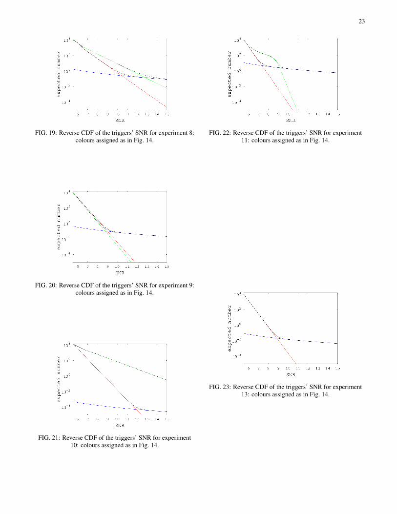
23
FIG. 19: Reverse CDF of the triggers’ SNR for experiment 8:colours assigned as in Fig. 14.
FIG. 20: Reverse CDF of the triggers’ SNR for experiment 9:colours assigned as in Fig. 14.
FIG. 21: Reverse CDF of the triggers’ SNR for experiment10: colours assigned as in Fig. 14.
FIG. 22: Reverse CDF of the triggers’ SNR for experiment11: colours assigned as in Fig. 14.
FIG. 23: Reverse CDF of the triggers’ SNR for experiment13: colours assigned as in Fig. 14.
24
2. Direct comparison
In Figs. 24, 25, 26, 27, 28, 29, 30, 31, 32, and 33 we presentplots of the direct comparison between actual FAP and theFAP estimations from all methods.
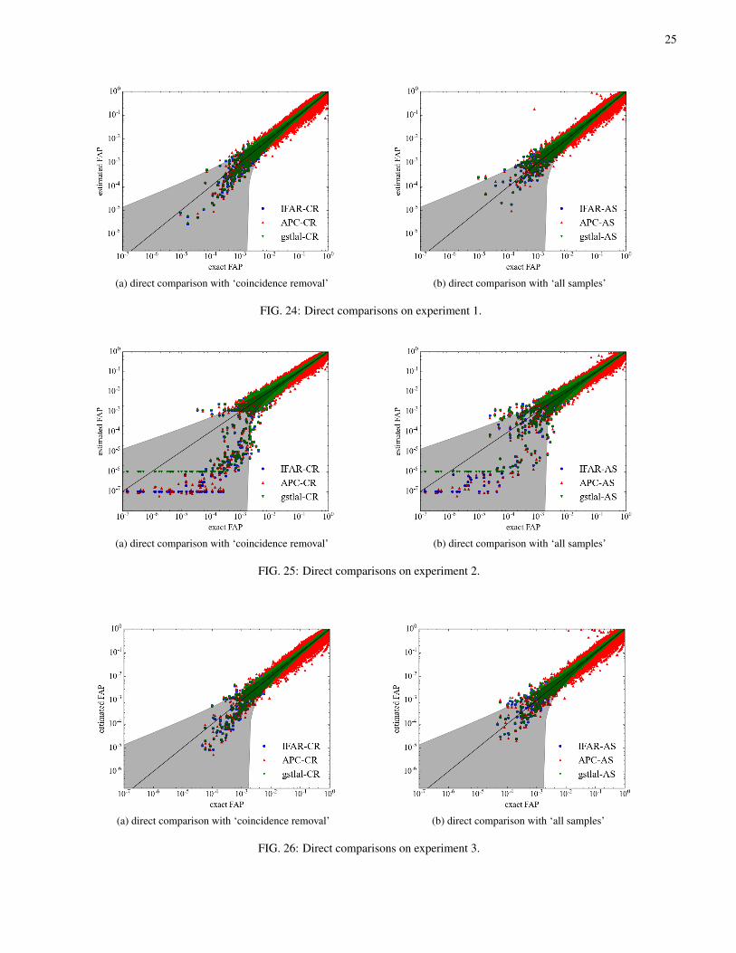
25
(a) direct comparison with ‘coincidence removal’ (b) direct comparison with ‘all samples’
FIG. 24: Direct comparisons on experiment 1.
(a) direct comparison with ‘coincidence removal’ (b) direct comparison with ‘all samples’
FIG. 25: Direct comparisons on experiment 2.
(a) direct comparison with ‘coincidence removal’ (b) direct comparison with ‘all samples’
FIG. 26: Direct comparisons on experiment 3.
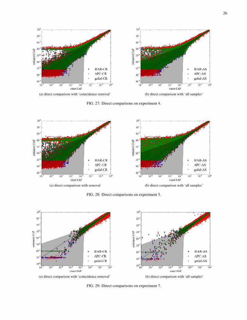
26
(a) direct comparison with ‘coincidence removal’ (b) direct comparison with ‘all samples’
FIG. 27: Direct comparisons on experiment 4.
(a) direct comparison with removal (b) direct comparison with ‘all samples’
FIG. 28: Direct comparisons on experiment 5.
(a) direct comparison with ‘coincidence removal’ (b) direct comparison with ‘all samples’
FIG. 29: Direct comparisons on experiment 7.

27
(a) direct comparison with ‘coincidence removal’ (b) direct comparison with ‘all samples’
FIG. 30: Direct comparisons on experiment 8.
(a) direct comparison with ‘coincidence removal’ (b) direct comparison with ‘all samples’
FIG. 31: Direct comparisons on experiment 10.
(a) direct comparison with ‘coincidence removal’ (b) direct comparison with ‘all samples’
FIG. 32: Direct comparisons on experiment 12.
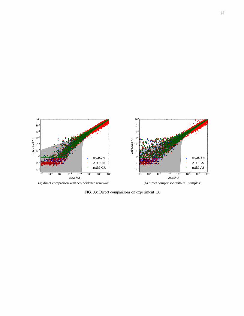
28
(a) direct comparison with ‘coincidence removal’ (b) direct comparison with ‘all samples’
FIG. 33: Direct comparisons on experiment 13.
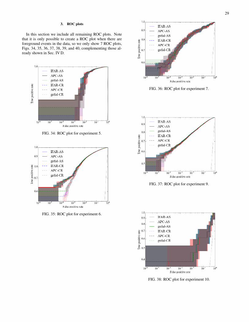
29
3. ROC plots
In this section we include all remaining ROC plots. Notethat it is only possible to create a ROC plot when there areforeground events in the data, so we only show 7 ROC plots,Figs. 34, 35, 36, 37, 38, 39, and 40, complementing those al-ready shown in Sec. IV D.
FIG. 34: ROC plot for experiment 5.
FIG. 35: ROC plot for experiment 6.
FIG. 36: ROC plot for experiment 7.
FIG. 37: ROC plot for experiment 9.
FIG. 38: ROC plot for experiment 10.
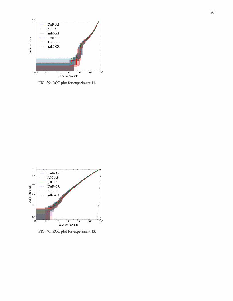
30
FIG. 39: ROC plot for experiment 11.
FIG. 40: ROC plot for experiment 13.