System - DiVA portal

A System Identi�cation Software Tool for General

MISO ARX�type of Model Structures

P� Lindskog

Department of Electrical Engineering

Link�oping University

S�� Link�oping

SWEDEN

Email lindskog�isy�liu�se

December ��

Abstract� The typical system identi�cation procedure requires powerful and versatile softwaremeans� In this paper we describe and exemplify the use of a prototype identi�cation softwaretool� applicable for the rather broad class of multi input single output model structures withregressors that are formed by delayed in� and outputs� Interesting special instances of this modelstructure category include� e�g�� linear ARX and many semi�physical structures� feed�forward neuralnetworks� radial basis function networks� hinging hyperplanes� certain fuzzy structures� etc�� as wellas any hybrid obtained by combining an arbitrary number of such approaches�

Keywords� System identi�cation software tools� matlab� MISO systems� linear and nonlinearARX structures� parameter estimation� simulation�

� Introduction

System identi�cation concerns the problem of designing mathematical models of dynamical systemsbased on observed data �� After experiment design and data pre�processing �detrending�removing outliers� etc� � the problem can be split into two parts� model structure selection followedby parameter estimation�To facilitate these steps in practice� general and powerful software tools of various kinds are

needed� In this paper we present and illustrate the use of a prototype matlab �� software pack�age� customized for unconstrained or constrained parameter estimation within the general multiinput single output ARX model structure class� This class involves all �linear as well as nonlin�ear structures that generate an output �a prediction based on input�output measurements thatare known at time t� The only technical restriction imposed on the model structure is that itmust be possible to compute the derivatives of the predictor with respect to all its parameters� atleast numerically� This is usually the case for linear ARX structures �� most semi�physicalstructures �� standard feed�forward neural networks �� feed�forward radial basisfunction networks �� hinging hyperplanes �� Takagi�Sugeno type of fuzzy model struc�tures �� etc�� as well as for any conceivable combination of these approaches�It is true that some of these structures are handled by commercial matlab toolboxes� like the

system identi�cation toolbox �� the neural network toolbox �� or the fuzzy logic toolbox ��although none of these packages cover the general ARX case� The system identi�cation toolboxis� e�g�� designed for linear model structures� whereas the fuzzy toolbox is tailored for certainfuzzy descriptions� Another important restriction is that these tools do not support constrained

estimation� which means that a priori known parameter restrictions cannot be guaranteed in theestimated models� However� such knowledge can be incorporated and dealt with using the opti�mization toolbox �� but there the principal problem is that neither simulation nor any othervalidation procedures are included� Altogether� these limitations have triggered the developmentof the software tool discussed below�The paper is organized as follows� In Section � we brie�y discuss the system identi�cation

problem� focusing mainly on structural issues as well as algorithms that are implemented� Basedon this material� Section addresses the use of the developed software tool� Then� Section �goes through a rather simple application example showing the possibilities of this package� Someconclusions and possible extensions are �nally provided in Section ��

� System identi�cation basics

This section reviews some basic identi�cation issues� starting next with main ingredients andnotation� In Section �� we concentrate on the choice of model structure� and in Section �� somesuitable parameter estimation algorithms are presented�

�� Main components and notation

The identi�cation procedure is in practice highly iterative and made up of three main ingredients�the data� the model structure and the selection criterion� all of which to some degree involvedecisions of subjective nature�

The data ZN� The natural starting point of any identi�cation session is the data� which willdepend both on the true system and on the experimental conditions� By the row vector

z�t� ��y�t� u��t� � � � um�t�

� � R��m �

we denote one speci�c data sample at time t collected from a system having one output andm inputsignals� i�e�� we consider a multi input single output �MISO system� This restriction is mainly forease of notation and the extension to multi output �MIMO systems is fairly straightforward� see�e�g�� Stacking N consecutive samples on top of each other gives the data matrix

ZN ��z��T z��T � � � z�N�T

�T � RN��m� � ��

where z�j�T is the transpose of the vector z�j��It is of course crucial that the data re�ect the important features of the underlying system�

In reality� and especially for complex systems� this requires carefully designed experiments� Herewe will not consider such design issues� but assume that the data have been collected in thebest possible way� The usual next step of pre�treating data in di�erent manners� like detrending�removing outliers� special �ltering� and so forth� is not covered either� for such procedures we referto the system identi�cation toolbox ��

The model structure g��t�� A general MISO model structure can be written

�y�tj�� g��t�� R� �

where �y�tj�� accentuates that the function g�� is a predictor� i�e�� it is based on signals that areknown at time t� The predictor structure is ensured by the regressor ��t�� which maps outputsignals up to index t � � and input signals up to index t to an r dimensional regression vector�This vector is often of the form

��t� ��y�t� �� y�t � k� u��t� � � � u��t� k��

um�t� � � � um�t� km��T� ��

although in general its entries can be any at time t computable combinations of input�output

�

Experimentdesign

Pre�treatdata

UN

ZN g��t�� VN�ZN��

Model

OK � accept model�

Choosemodel

structure

Chooseperformancecriterion

Priorsystemknowledge�physics�linguistics�etc�

DParameter estimation

Validatemodel Not OK � revise�

Not OK � revise prior�

Figure �� The system identi�cation loop� Grey boxes mark issues handled by the developed software� atleast partly� Grey arrows mark the use of prior knowledge�

signals� measured as well as predicted or simulated ones� The mapping g�� from Rr to R is

parameterized by � � D � Rd � with the set D denoting the set of values over which � is allowed to

range due to parameter restrictions� With this formulation� the work on �nding a suitable modelstructure splits naturally into two subtasks� both possibly being nonlinear in nature�

� the choice of dynamics� i�e�� the choice of regression vector ��t�� followed by

�� the choice of static mapping g�� The performance criterion VN�ZN�� Measured and model outputs never match perfectlyin practice� but di�er as

��tj�� y�t� � �y�tj��

where ��tj�� is an error term re�ecting unmodeled dynamics on one hand and noise on the otherhand� An obvious modeling goal must be that this discrepancy is �small� in some sense� This isachieved by the selection criterion� which ranks di�erent models according to some pre�determinedcost function� The selection criterion can come in several shapes� but pre�dominant in this businessis to use a quadratic measure of the �t between measured and predicted values�

VN�ZN��

N

NXt��

�

��y�t� � �y�tj��

��

�

N

NXt��

�

��tj��

Once these three issues are settled we have implicitly de�ned the searched for model� It then�only� remains to estimate the parameters � and to decide whether the model is good enough ornot� If the model cannot be accepted some or even all of the entities above have to be reconsidered�in the worst possible case one must start from the very beginning and collect new data� Thisworking procedure � the system identi�cation loop �� is reproduced in Figure �

�� General ARX model structures

The class of general �linear as well as nonlinear ARX model structures is speci�ed by the type

of regressors ��t� being used in the predictor � � see �� The requirement is that all regressorsshould be formed by measured signals only� i�e�� in the MISO system case the regressors shouldbe solely composed of signals of the kind involved in �� Notice that the general FIR modelstructure� which uses old inputs u�t � k� as regressors� is just a specialization of this category�However� structures with regressors based on previous outputs from the model itself� predictedor simulated ones� do not �t into this framework� More to the point� the current version of thesoftware is not able to handle general output error �OE structures� which use simulated insteadof measured outputs� general ARMAX structures� which besides measured in� and outputs usepredicted outputs� nor can it deal with general Box�Jenkins �BJ structures� which use measuredinputs as well as measured� predicted and simulated outputs�Despite these restrictions� there is still a large �ora of model structure possibilities� Some of

these are presented next�

Linear ARX structures� The linear MISO ARX model structure is simply

�y�tj�� g��t��

nXj��

�j�j�t� � �T��t��

where ��t� is given by ��

Linear structures with orthonormal basis functions� In a linear ARX structure we alwaysrun the risk of arriving at an unstable model� This can be avoided by using �ltered inputs asregressors

�y�tj�� g��t��

nXj��

�jBj�u�t��

where all the Bj��s are linear stable �lters� For a number of reasons� see� e�g�� these pre��ltersare often chosen to form an orthonormal set of basis functions in H�� This is the casefor the choice Bj�u�t�� u�t � j�� which results in the linear FIR model structure� To reduce thenumber of basis functions needed to arrive at useful models it is here appealing to try other choicesof Bj�� This is the main idea behind orthonormal Laguerre and Kautz �lters �� which� toreduce the number of parameters to estimate� utilize prior knowledge about the dominating timeconstants of the underlying system�

Semi�physical structures� Another approach bene�tting from partial prior system knowledgeis so called semi�physical modeling� There the basic idea is to use physical insight about thesystem so as to come up with certain nonlinear �and physically motivated combinations of theraw measurements ZN� These combinations � the new inputs and outputs � are then subjected tostandard model structures�More precisely� from an estimation viewpoint �see the next section it is often desired to have

a predictor of the form �� with all nonlinearities appearing in the regressor ��t� �here composedof measured signals only � The regressors to include in the structure are of course determined ona case by case basis� For example� to model the power delivered by a heater element �a resistor �an obvious physically motivated regressor to employ would be the squared voltage applied tothe resistor� In other and more complicated modeling situations the prior is given as a set ofunstructured di�erential�algebraic equations� To then arrive at a model of the form �� requiresboth symbolic and numeric software tools as is demonstrated in ��

Feed�forward neural networks� When the system shows a nonlinear behavior� a rather com�mon modeling approach is to try nonlinear predictor structures resembling a function expansion

�y�tj�� g��t��

nXj��

jgj��t��j��j��

�T �

��T �

T�T��

�

where gj�� is called a basis function� and j� �j and �j are weight �or coordinate � scale �ordirection � and position �or translation parameters �� With basis functions of the form

gj��t��j� �j� � ��Tj ��t� � �j��

where �� is an activation function in one variable having parameters �j � Rr and �j � R� we geta ridge construction �� Notice that the ridge nature has nothing to do with the choice of ��It is attributed to the fact that �� is constant for all regression vectors in the subspace where�Tj ��t� is constant� thus forming a ridge along that direction� A standard choice of activationfunction is the sigmoid function

��x� � �x� ��

� � e�x� ��

which� with regressors �� yields a sigmoid one hidden layer feed�forward neural network �� Many di�erent generalizations of this basic structure are possible� For example� step� piecewise lin�ear and hyperbolic tangent functions �� are other activation functions sometimes being advocatedin the literature� A network with several hidden layers is also readily obtained if the �� blocksare again weighted� thresholded and fed through a new layer of �� blocks� However� recurrent�as opposed to feed�forward neural networks do not belong to the considered model class� owingto that network internal signals are there fed back to the regression vector�

Hinging hyperplanes� Breiman �� has recently suggested a hinging hyperplane model struc�ture� having V�shaped basis functions rather than� e�g�� sigmoidal ones� In �� it is shown thatthe original hinging hyperplane description is equivalent to

�y�tj�� g��t��

nXj��

�Tj ��t�ISj��t�� T��t��

where the indicator function ISj��t�� is if ��t� � Sj� and zero otherwise� thus splitting theregression space into smaller regions� The overall parameter vector is here composed of n � �

sub�vector elements� each containing r parameters� It is not hard to verify that this is also a seriesexpansion of ridge type� see ��

Feed�forward radial basis function networks� Another frequently used class of basis func�tions is of radial type �� which do not show the ridge directional property but have truelocal support� The series expansion �� with regressors �� is then composed of elements

gj��t��j��j� � ��jj��t� � �jjj��j

��

where the weighted norm �j specify the scaling of �� Even if a few di�erent radial functionshave been suggested in the literature� see� e�g�� it is often chosen to be a Gaussian

��jjxjjj��j

� � e��xTj �

��jxj � ��

where xj � ��t��j� �j � Rr � and ��j � ��Tj �j� �j � Rr � with �j and �j representing the meanand the covariance of the Gaussian� respectively�

Fuzzy model structures� A composition �tensor product in �� is obtained whenever ridgeand radial constructions are combined when forming the basis functions of �� The most extreme�yet often used� composition

gj��t��j��j� �

rYk��

gj�k��k�t��j�k��j�k� ��

is the construction often employed in fuzzy identi�cation �� where a set of linguisticrules� like �If temperature�t � �� is high and �ow�t � �� is low then temperature�t� is high�� is

�

translated into a mathematical representation � a model structure� A very common translationresults in the Mamdani fuzzy model structure �consult� e�g�� for the derivation

�y�tj��

n�Xj��

� � �

nrXjr��

j�� jr �rY

k��

�Ajk�k��k�t��jk�k��jk�k�

n�Xj��

� � �

nrXjr��

rYk��

�Ajk�k��k�t��jk�k� �jk�k�

� ��

which di�ers from the other series expansions in that the parameters here can be linguisticallyinterpreted� Another di�erence is the denominator part� which merely performs a normalization�Notice also that the labeling in �� is just a convenient grid�oriented relabeling of the basis func�tions gj�k�� or� as they are called in a fuzzy context� membership functions �Ajk�k

�� Thesecan in principle be any functions returning values in the interval �� e�g�� sigmoids� Gaussians�piecewise linear functions� etc�A natural extension of structure �� is to allow slightly more complex local models than just

constants j�� jr � One straightforward idea is to replace the constants by local ARX predictors��Tj�� jr��t� � �j�� jr � This gives the Takagi�Sugeno fuzzy model family ��

�y�tj��

n�Xj��

� � �

nrXjr��

��Tj�� jr��t� � �j�� jr

� � rYk��

�Ajk�k��k�t��jk�k��jk�k�

n�Xj��

� � �

nrXjr��

rYk��

�Ajk�k��k�t��jk�k� �jk�k�

� ��

which indeed has much in common with gain scheduling techniques�

Other structures� The story of nonlinear series expansions of the form �� does not end here�Model regression trees �� a composition � wavelet networks �� radial type � kernel esti�mators �� radial type � as well as some other structures �� also belong to this versatile category�Observe that these methods are local in the sense that they involve basis functions having localsupport� i�e�� each gj�� is in principle only active in certain parts of the total regression space�Global nonlinear basis functions� like Hammerstein structures �� but also Wiener �� and

Volterra �� functional series realizations� fall within the general ARX framework� In fact� so doesany hybrid structure obtained by combining any of the above structures� see Section ��

�� General parameter estimation techniques

After having determined the model structure to apply� the next step is to use input�output data toestimate what is still unknown� It is here useful to divide the estimation needs into three categories�

Structure estimation� This is the case when the type of model structure approach to use hasbeen decided� but where the size� i�e�� the number of basis functions n to employ� is estimated�This typically leads to a combinatorial optimization problem� which in complexity grows rapidlywith the problem size� The present software version does not consider structure estimation� it isassumed that n is determined by the user in one way or another�

Nonlinear�in�the�parameters estimation� Having decided the size of the model structure itremains to �nd reasonable parameter values �� With the scalar loss function �� as the performance

criterion the parameter estimate ��N is given by

��N � argmin��D

VN�ZN��

where �argmin� is the operator that returns the argument that minimizes the loss function� Thisis a very important and well�known problem formulation leading to prediction error minimization

�

�PEM methods� The type of PEM algorithm to apply depends on whether the parameters �enter the model structure in a linear or a nonlinear way� The latter situation leads to a nonlinearleast�squares problem� and appears� e�g�� in series expansions �� that are equipped with unknowndirection � or translation � parameters�

Linear�in�the�parameters estimation� When all parameters enter the structure in a linearfashion one usually talks about a linear least�squares problem� This is the case for structures �� and �� but also for series expansions �� if only coordinate parameters � are to be estimated�

It should be emphasized that the complexity of the estimation problem decreases in the listedorder� yet at the price of that the amount of prior needed to arrive at a useful model typicallyincreases� With these preliminary observations� we next present some di�erent minimization algo�rithms� unconstrained as well as constrained ones�

�� Unconstrained linear least�squares estimation

The parameters of an unconstrained linear least�squares structure �a linear regression can beestimated e�ciently and analytically by solving the normal equations

��t��t�T��N � ��t�y�t� ��

for t � �� N� The optimal parameter estimate is simply

��N �

�NXt��

��t��t�T

��NXt��

��t�y�t� � R��N fN� ��

provided that the inverse of the d � d regression matrix RN exists� For numerical reasons thisinverse is rarely formed� but instead the estimate is computed via so called QR� or singular valuedecomposition �SVD �� which both are able to handle rank de�cient regression matrices� Theformer approach is� e�g�� applied in the matlab �n��operator �� utilized in our implementation�

�� Unconstrained nonlinear least�squares estimation

When the parameters appear in a nonlinear fashion the typical situation is that the minimum ofthe loss function cannot be computed analytically� Instead we have to resort to certain iterativesearch routines� most of which can be seen as special cases of Newton�s algorithm �see among manyothers ��

��i��

N � ��i�

N �hV��N�ZN�

��i�

N �i��

V�N�ZN� ��

�i�

N � � ��i�

N � ��i�

N �ZN� ��i�

N ��

where ��i�

N � Rd is the parameter estimate at the i�th iteration� V�N�� Rd is the gradient of

the loss function and V��N�� Rd�d the Hessian of it� both computed with respect to the current

parameter vector� More speci�cally� the gradient is given by

V�N�ZN� ��

�i�

N � � ��

N

NXt��

J�tj��i�

N ��tj��i�

N ��

with J�tj��i�

N � � Rd being the Jacobian vector

J�tj��i�

N � �

��y�tj��

�i�

N �

��i�

�

� � ��y�tj��

�i�

N �

��i�

d

�T� ��

and di�erentiating the gradient with respect to the parameters yields the Hessian

�

V ��N�ZN�

��i�

N � ��

N

NXt��

��J�tj��i�N �J�tj��

�i�

N �T ��J�tj��

�i�

N �

��i�

N

��tj��i�

N �

A � ��

Simply put� Newton�s algorithm searches for the new parameter vector along a Hessian modi�edgradient of the current loss function�The availability of derivatives of the loss function with respect to the parameters is of course of

paramount importance in all Newton�based estimation schemes� In case arbitrary �though di�er�entiable predictor structures are considered these may very well be too hard to obtain analyticallyor too expensive to compute� One way around this di�culty is to numerically approximate thederivatives by �nite di�erences� The simplest such a method is just to replace each of the delements of the Jacobian by the forward di�erence

Jj�tj��i�

N � ��y�tj��

�i�

N �

��i�

j

� �y�tj��i�

N � hjej� � �y�tj��i�

N �

hj� ��

with ej being a column vector with a one in the j�th position and zeros elsewhere� and with hjbeing a small positive scalar perturbation� Because the parameters may di�er substantially inmagnitude it is here expedient to individually choose these perturbations� A typical choice is

hj �p�max�hmin�

��i�j �� where � is the relative machine precision and hmin � � is the smallestperturbation allowed� consult �� for further details on this� If a more accurate approximationis deemed necessary one can employ the central di�erence

Jj�t� ��i�

N � ��y�tj��

�i�

N �

��i�

j

� �y�tj��i�

N � hjej� � �y�tj��i�

N � hjej�

�hj� ��

at the cost of d additional function evaluations�It now turns out that the Newton update �� has some severe drawbacks� most of which are

associated with the computation of the Hessian �� First of all� it is in general expensive tocompute the derivative of the Jacobian� It may also happen that the inverse of the Hessian doesnot exist� so if further progress towards a minimum is to be made the update vector must beconstructed in a di�erent way� Also� even if the inverse exists it is not guaranteed to be positivede�nite� It may therefore happen that the parameter update vector is such that the loss functionactually becomes larger� Finally� although the parameter update vector is a descent one it can bemuch too large� locating the new parameters at a point with higher loss than what is currently thecase� The following �implemented three variants of �� are all safeguarded against these pitfalls�

Damped gradient method� Simply replace the Hessian by an identity matrix of appropriatesize� However� this does not prevent the update from being so large that also VN�� becomeslarger� To avoid such a behavior the updating is often complemented with a line search technique

��i�

N �ZN� ��i�

N � � ��i�V �N�ZN�

��i�

N ��

where � � ��i� � �� thereby giving a damped gradient algorithm� The choice of step length ��i� isnot critical� and the procedure often used is to start with ��i� � � and then repeatedly halve ituntil a lower value of the loss function is obtained�

Damped Gauss�Newton method� By skipping the second derivative term of the Hessian �� and including line search as above we get a damped Gauss�Newton algorithm with update vector

��i�

N �ZN� ��i�

N � � ��i�

�NXt��

J�tj��i�

N �J�tj��i�

N �T

��NXt��

J�tj��i�


N ��

which is of the same form as the linear least�squares formula �� The only trouble that can arisehere is that the �rst sum produces a matrix that is singular or so close to singular that the inversecannot be computed accurately�

�

Such a situation can be handled e�ciently via numerically reliable SVD computations �� asfollows� An equivalent matrix formulation of �� is

��i�

N �ZN� ��i�

N � � ��i�hJTNJN

i��JTNN� ��

where the matrix JN � RN�d and the column vector N � RN are constructed in the obvious way�If we make the reasonable assumption that N � d� i�e�� the number of measurements is larger thanthe number of parameters� then the Jacobian can be factored as ��

JN � U�VT� �

where U � RN�d and V � R

d�d are orthogonal matrices� and where � � Rd�d is a diagonal

matrix diag� �� d� �all elements lying outside the main diagonal are zero such that � � � � � � � � d � �� The k�s are called singular values and the construction as such isknown as singular value decomposition� As UT

U is an identity matrix it immediately follows that

JTNJN �

�U�V

T�T

U�VT � V�U

TU�V

T � V��VT� ��

If this matrix is singular� then it holds that one or more of the last �k�s are zero� and if it is closeto singular some of the �k�s will be small� Since the computation of the inverse becomes harderthe larger the quote ��

�d becomes it is reasonable to consider the s singular values for which

�� s is larger than� e�g�� the machine precision �� while zeroing the rest d� s entries� This gives

the approximation

JTNJN � V diag� ��

��

�s � ��

�VT �

from which the pseudo�inverse �or Moore�Penrose inverse is computed ashJTNJN

iy� Vdiag

�

��

��

�

�s� ��

�VT� ��

Now� replacing the inverse in the update �� by the pseudo�inverse has the e�ect that the sparameters in�uencing the criterion �t most are updated� whereas the rest d � s parameters areunchanged� This means that so called regularization is built into the method �see Section �� The damped Gauss�Newton algorithm is usually much more e�cient than the gradient method�

especially near the minimum where it typically shows similar convergence properties as the fullNewton algorithm ��

The Levenberg�Marquardt method� The Levenberg�Marquardt algorithm handles simulta�neously the update step size and the singularity problems through the update

��i�

N �ZN� ��i�

N � �

��NXt��

J�tj��i�

N �J�tj��i�

N �T

�� i�I

��NXt��

J�tj��i�


N ��

where the Hessian is guaranteed to be positive de�nite since ��i� � �� As is the case for the aboveprocedures� it can be shown that this update is in a descent direction� However� ��i� must becarefully chosen so that the loss function also decreases� Avoiding to repeatedly solve �� in thesearch for such a ��i�� we can again use the SVD �� which expanded with the ��i�I term becomes

JTNJN � ��i�I � V diag

� �� i�� i�� d � ��i�

�VT� ��

At this stage� the inverse is readily formed as before�hJTNJN � ��i�I

i�� V diag

�

�� i��

�

�� i��

�

�d � ��i�

�VT� ��

hence meaning that each line search iteration involves matrix multiplications only� Equation �� also provides useful insights in how the algorithm operates� A zero ��i� gives a Gauss�Newton step�

�

which close to the minimum is desired because of its tractable rate of convergence� By increasing��i� the inner diagonal matrix becomes more and more like a scaled identity matrix� and sinceVVT � I the update is essentially turned into a small gradient step�Various strategies for choosing ��i� have been suggested in the literature� two of which are

available in the developed software tool�

� The Marquardt method �� starts o� with a ��i� � � and attempts to reduce it �typically afactor � at the beginning of each iteration� but if this results in an increased loss� then the

step ��i� is repeatedly increased �typically a factor � until VN�ZN� ��i��

N � � VN�ZN� ��i�

N ��

�� Fletcher� see �� for the algorithmic details� has devised another rather �exible and moree�cient step length strategy that is based upon a comparison of the actual performance withwhat should be expected with a truly quadratic criterion� Even if this approach is morecomplex than the former one it often gives faster convergence� see ��

For ill�conditioned problems� �� recommends the Levenberg�Marquardt modi�cation� However�this choice is far less obvious when the pseudo�inverse is used in the Gauss�Newton update�

Stopping criteria� A last algorithmic issue to consider here is when to terminate the search� Intheory� V�

N�� is zero at a minimum� so an obvious practical test is to terminate once jV �N�� j is

su�ciently small� Another useful test is to investigate the relative change in parameters from oneiteration to another and terminate if this quantity falls below some tolerance level� The algorithmswill also terminate when a certain number of maximum iterations has been carried out� or if theline search algorithm fails to decrease the loss function in a predetermined number of iterations�It is worth stressing that the three schemes above all return estimates that are at least as

good as the starting point� Nonetheless� should the algorithm converge to a minimum� then it isimportant to remember that convergence needs not be to a global minimum but can very well beto a local one�

�� Constrained minimization

In quite a few modeling situations some or even all of the parameters have physical or linguisticsigni�cance� and hence D � R

d � To really maintain such a property it is necessary to take thecorresponding parameter restrictions into account in the estimation procedure� i�e�� constrainedoptimization methods are needed�Therefore assume that there are l parameter constraints collected in a vector

c�� c�� c�� cl��

�T � Rl � ��

where each cj�� is a well�de�ned function such that cj�� for j � �� l� thereby specifyinga feasible parameter region D� There exist quite a few schemes that handles such constraints� see�e�g�� An old but simple and versatile idea is to rephrase the original problem into a sequenceof unconstrained minimization problems for which a Newton type of method �here the gradientone can be applied without too much extra coding e�ort�This is the basic idea behind the barrier function estimation procedure� Algorithmically speak�

ing� the method starts with a feasible parameter vector ��

N � whereupon the parameter estimate isiteratively obtained by solving �each iteration is started with the estimate of the previous iteration

��k��

N � argmin��D

WN�ZN�� argmin��D

��VN�ZN�� k�

lXj��

��cj��

A � ��

where� typically� ��k� � ��k with k starting from � and then increasing by for each iterationuntil convergence is obtained� In order to maintain a feasible estimate the barrier function ��

�

is chosen so that an increasingly larger value is added to the objective function WN�� as theboundary of the feasibility region D is approached from the interior� at the boundary itself thisquantity should be in�nite� The barrier function is sometimes chosen to be the inverse barrier

function

��ck�� c��k ��

although more often the log barrier function

��ck�� log�ck��

is used� as it usually do a better job ��At this stage one may wonder why it is not su�cient to set ��k� to a much smaller value in the

beginning� One reason is that if the true minimum is near the boundary� then it could be di�cultto minimize the overall cost function because of its rapidly changing curvature near this minimum�thus giving rise to an ill�conditioned problem� One could also argue that the method is too complexas an outer iteration is added� This is only partially true as the inner estimate �especially at the�rst few outer iterations needs not be that accurate� A rule of thumb is to only perform some�ve iterations in the inner loop� Finally� the outer loop is terminated once the parameter updateis su�ciently small or when a number of maximum outer iterations has been carried out�

�� The bias�variance trade�o

In a black box identi�cation setting the basic idea is to employ a parameterization that covers anas broad system class as possible� In practice� and especially for nonlinear series expansions �� the typical situation is that merely a fraction of the available �exibility is really needed� i�e�� theapplied model structures are often over�parameterized� This fact� possibly in combination with aninsu�ciently informative data set ZN� leads to ill�conditioning of the Jacobian and the Hessian�This observation also suggests that the parameters should be divided into two sets� the set ofspurious parameters� which do not in�uence the criterion �t that much� and the set of e�cient

parameters� which do a�ect the �t� Having such a decomposition it is intuitively reasonable totreat the spurious or redundant parameters as constants that are not estimated� The problem withthis is that it is in general hard to make such a decomposition beforehand�However� using data one can overcome the ill�conditioning problem and automatically un�

veil an e�cient parameterization by incorporating regularization techniques �or trust region tech�niques �� When such an e�ect is built into the estimation procedure� as in the Levenberg�Marquardt algorithm� we get so called implicit regularization� as opposed to explicit regularization�which is obtained by adding another penalty term to the criterion function� e�g�� as

WN�ZN�� VN�ZN�� k�lX

j��

��cj��

�

��

where � � � is a small user�tunable parameter ensuring a positive de�nite Hessian and �� Rdis some a priori determined parameter vector representing prior parameter knowledge� Here theimportant point is that a parameter not a�ecting the �rst term that much will be kept close to ��

by the last term� This means that the regularization parameter � can be viewed as a thresholdthat labels the parameters to be either e�cient or spurious �� A large � simply means that thenumber of e�cient parameters d� becomes small�From a system identi�cation viewpoint regularization is a very important means for addressing

the ever present bias�variance trade�o�� as is emphasized in �� There it is shown� under fairlygeneral assumptions� that the asymptotic criterion mis�t essentially depends on two factors thatcan be a�ected by the choice of model structure� First we have the bias error� which re�ects themis�t between the true system and the best possible approximation of it� given a certain model

structure� Typically� this error decreases when the number of parameters d increases� The otherterm is the parameter variance error� which usually grows with d but decreases with N� There isthus a clear trade�o� between the bias and the variance contributions�At this point� suppose that a �exible enough model structure has been decided upon� Decreasing

the number of parameters that are actually updated �d� by increasing � is bene�cial for the totalmis�t as long as the decrease in variance error is larger than the increase in bias error� In otherwords� the purpose of regularization is to decrease the variance error contribution to a level whereit balances the bias mis�t�

� Software

We are now in a position to discuss the developed matlab software and its functionality� Ulti�mately� we would like to have an easy to use� easy to extend� versatile and interactive softwaretool� preferably of the kind shown in Figure ��

Numerics

Data pre�processing

Structure estimation

Validation procedures

Parameter estimation

� � �

Low level services

Computational

services

Symbolics

Identi�ability�

� � �

Model structureselection

Data base systems

Bookkeeping

� � �

Other services

Documentation

� � �

Modeling aid�� bond graphs� object orientedtools

User inter�

action level

Supervisor

Graphical userinterface GUI� � � �

Help systems

Knowledge�basedsystems KBS� � � �

High leveluser services

Interfacing language

Nonparametric alg� Documentation

Figure �� Suitable structure of a general system identi�cation software tool� The present software versionis limited to numeric computations� Further details on and discussions about the other blocks can be foundin� e�g��

The prototype package developed so far addresses only a portion of the numeric needs� However�integrating further tools from Figure � is rather straightforward� �rstly due to that matlab includesmeans for creating graphical user interfaces �GUI � and� secondly� due to that it enables symboliccomputations via the symbolic toolbox �� Even if matlab does not yet include data base orknowledge�based systems� it is likely that such integrations can be made rather painlessly�After this short introduction� we next focus on what can be done with the current software�

Sections �� discuss how to describe the data� general ARX predictors� parameter constraints�etc�� whereas Sections �� and �� concentrate on parameter estimation and validation� respectively�

�� Describing the data

The output�input data� Z � ZN� is assumed to be given as a matrix of the form �� To relive theuser from the burden of having to work with Z�matrix indexes when specifying the model structure�

�

the individual data columns are named using a string Zd�

Zd � ��y�t��u��t��um�t��

The independent variable t as well as the measured variables can in principle be given arbitrarynames� preferably tailored to the application�

Example � �solar heated house�� In the solar heated house example of �� there are threemeasured signals� T�t� � temperature in a heat storing magazine at time t the output� I�t� � thesun radiation a non�controllable input� and u�t� � the voltage fed to a pump generating a heat ow to the magazine a controllable input� The data of this system is described by

Zd � ��T�t��I�t��u�t��

�� Specifying model structure

The model structure is also described by a string Ms that� when evaluated� returns a one step aheadprediction � � The string Ms is allowed to involve parameters� which are always speci�ed via thereserved parameter name P � a column vector with d entries� and measurements �� correspondingto Zd� These entities can be combined using simple operators and�or more complex functions �e�g��own�de�ned m��les � thus enabling general MISO ARX predictor descriptions� The used operatorsand functions should be well�de�ned and chosen so that the Jacobian �� can be computed�Another important requirement is that the operators and functions should be able to operate onand return vectors� This is readily obtained through matlab�s �dotted� array operators� �� and � �� The following example clari�es these points�

Example � �solar heated house� continued�� After some modeling and symbolic computa�tions� see �� it turns out that a suitable model structure for describing the solar heated house�or actually the temperature in the magazine� is

�T�tj�� T��t� � ��T�t� �� I�t� ��u�t � �� T�t� ��u�t � ��

� ��T�t� ��u�t � �� T�t� ��u�t � ��

u�t � ��

T�t� ��u�t � ��

u�t � ��

where � � P � R � This model structure is here entered as

Ms � ��P��T�t�� P��I�t��u�t�� P��T�t��u�t��

�P��T�t��u�t�� P��T�t��u�t��u�t��

�P��T�t��u�t��u�t��

Notice how the �dotted� operators are used for vector multiplication and division� To get a well�de�ned predictor it must also be required that u�t� �� for t � �� N� Using regressor screeningtechniques� a simpli�ed and �better� model structure is

�T�tj�� T��t� � ��T�t� �� I�t� ��u�t � ��

which simply can be entered as

Ms � �P��T�t�� P��I�t��u�t��

�� Specifying parameter constraints

The parameter constraints Con � c�� are assumed to be of inequality type� cj�� forj � �� l� thereby specifying the feasible parameter space D� Each cj�� is assumed to be well�de�ned� and entered as a string� The l inequalities are subsequently put together in a string matrixusing the matlab command mat�str�c�� c�� Observe that mat�str at most can becalled with � string arguments� However� each such argument can itself be a string matrix� whichmeans that arbitrary large string matrices can be created� and hence D can be realized�

Example � �parameter constraints�� Suppose that � � P � R� are such that

��

The following �ve lines of matlab code bring about these restrictions�

c� � �P��

c� � �� P��

c� � �P�� P��

c� � �P�� P�� P��

Con � mat�str�c��c��c��c��

�� Specifying explicit regularization

Explicit regularization as described and discussed in Section �� can be speci�ed through a stringEreg� Although Ereg is not restricted to a penalty term of the form added in �� it must stillbe an expression in parameters P only� It must also be constructed so that it always produces apositive scalar value�

Example �explicit regularization�� Assume that � � P � R� � Regularization towards

�� and �� can be speci�ed through

Ereg � ��P�� P�� P��

with a belief factor � � �� It should be pointed out that the choice of � is in general not an easyone� The situation becomes even more intrinsic if the terms are individually weighted� e�g�� as

Ereg � ��P�� P�� P��

This particular choice of weights means in principle that the relative belief in that �� is close to �is high� whereas the belief in that �� is close to �� is relatively low�

�� Fuzzy speci�c facilities

Although the developed software handles general MISO ARX predictors� the aim of the codingactivities was in the beginning to enable and promote fuzzy identi�cation �� Central objects insuch and other type of fuzzy logic applications are fuzzy sets and membership functions �MF � orbasis functions� Mathematically speaking� the de�nition is as follows ��

Denition � �fuzzy set�� If u is an element in the universe of discourse U � R� then a fuzzyset A in U is the set of ordered pairs

A � f�u� �A�u�� u � Ug� ��

where �A�u� is a membership function carrying an element from U into a membership valuebetween � no degree of membership and � full degree of membership�

The purpose of a fuzzy set A is to connect a vague linguistic value� like low� medium� or high� toa precise mathematical characterization via the MF� As noted earlier� the membership functioncan be any function producing a value between � and � Besides a singleton MF �see below � thecurrent implementation includes three common classes of MFs� all being convex in nature ��i�e�� the MFs are of the form �increasing�� decreasing�� or �bell�shaped�� These classes are heretermed Zadeh�formed MFs� network�classic MFs� and piecewise linear MFs� computed as follows�

Singleton MF�

�A � mfsing��

�� u � � u � U�� otherwise�

�

Zadeh�formed MFs�

Z�function� �A � mfz�u� ��

��

� u � ��

� � �

u� ��

��

�� u � ��

��

�

u � ��

��

��

�� u � ��

� u � ��

S�function� �A � mfs�u� �� mfz�u� ��

�function� �A � mfpi�u� ��

��mfs�u� �� u � ��

� �� u � ��

mfz�u� �� u � ��

Network�classic MFs�

Sigmoid� �A � mfsig�u� ��

� � e��u��

Gaussian� �A � mfgauss�u� �� e��

u��

�

�

General bell� �A � mfbell�u� �� a� ��

� �u��

�

�a �Prod� of � sigmoids� �A � mfpsig�u� ��

�

�� e��u��

�

�� e��u��

Piecewise linear MFs�

Open left function� �A � mfl�u� �� max

min

�� u

��

��

��

Open right function� �A � mfr�u� �� max

min

u � ��

��

��

��

Triangular function� �A � mftri�u� �� max

min

u � ��

�� u

��

��

��

Trapezoidal function� �A � mftrap�u� �� max

min

u� ��

��

�� u

��

��

��

Figure shows typical appearances of these MFs� If desired the user can design other MFs viaown�de�ned m��les� These functions should always be constructed to operate on vectors� i�e�� ifthe input argument u is a column vector� then the result should also be a column vector havingthe same number of entries as u�Another key concept in fuzzy modeling and control is so called linguistic variables� which can

be assigned certain linguistic values� each being described by an appropriate MF� In a generalizedform �cf� �� such a variable is here speci�ed by a string

Lv � ��Name�Type�Universe�Unit�Vlist�D��

where

� Name is the name of the linguistic variable� e�g�� temperature�t�� speed�t�� etc�

�� Type is either P if Lv is used in the rule premise �see below � or C if it is used in a ruleconsequent part� This information is only used when plotting MFs�

� Universe �U speci�es the domain where Lv is de�ned� Entered as minmax� e�g��

�� Unit is the physical measurement unit of Lv� e�g�� m�s�

�� Vlist is a complete list of linguistic values that can be assigned to the linguistic variable Lv�Each such value is coupled to a suitable MF using the syntax

�

a� Singleton MF� b� Zadeh�formed MFs�

�

�

U

mfsing��

�

�

�

U

��

mfz�u� ��

��

��

��

�

�

U

��

mfs�u� ��

��

��

��

�

�

U

��

mfpi�u� ��

��

��

��

��

��

��

c� Network�classic MFs�

�

�

U

�

mfsig�u� ��

� �

� � �

�

�

�

U

�

mfgauss�u� ��

� �

� � �

�

�

�

U

�

mfbell�u� ��a� ��

a � �

� � �

��

a

�

�

U

��

mfpsig�u� ��

��

��

��

��

��

��

��

d� Piecewise linear MFs�

�

�

U

��

mfl�u� ��

��

��

��

�

�

U

��

mfr�u� ��

��

��

��

�

�

U

��

mftri�u� ��

��

��

��

��

��

�

�

U

��

mftrap�u� ��

��

��

��

��

��

��

Figure �� Typical results of available MFs when U � ��

Vlist � �V��MF��V��MF��Vn�MFn��

For example� if Lv � �speed�t�� then a possible list of linguistic values are

Vlist � �low�mfsig�u��medium�mfgauss�u��high�mfsig�u��

�� D de�nes the physical measurement equivalent of Lv� If Lv � �speed�t�� then� e�g�� D �

�v�t�� where v�t� is assumed to be a measured signal speci�ed in Zd� It can also be amore complex expression involving several measured signals�

The r�� linguistic variables �r ones appear in the rule antecedents and one appears in the ruleconsequences used in a fuzzy application are �nally collected in one single string of the form

Lvlist � �Lv��Lv��Lvr��

where each LVj is given by �� See Section �� for a more continuous example of this�Four functions operating on linguistic variables or list of such variables are implemented�

� islv�Lv� returns if Lv is a linguistic variable� Otherwise � is returned�

�� islvlist�Lvlist� returns if Lvlist is a list of linguistic variables� Otherwise � isreturned�

�

� getlv�Lv�D��D�� returns Lv speci�c information� like its name� universe� etc� What infor�mation to retrieve is speci�ed by D� and D�� Lv can also be a list of linguistic variables�

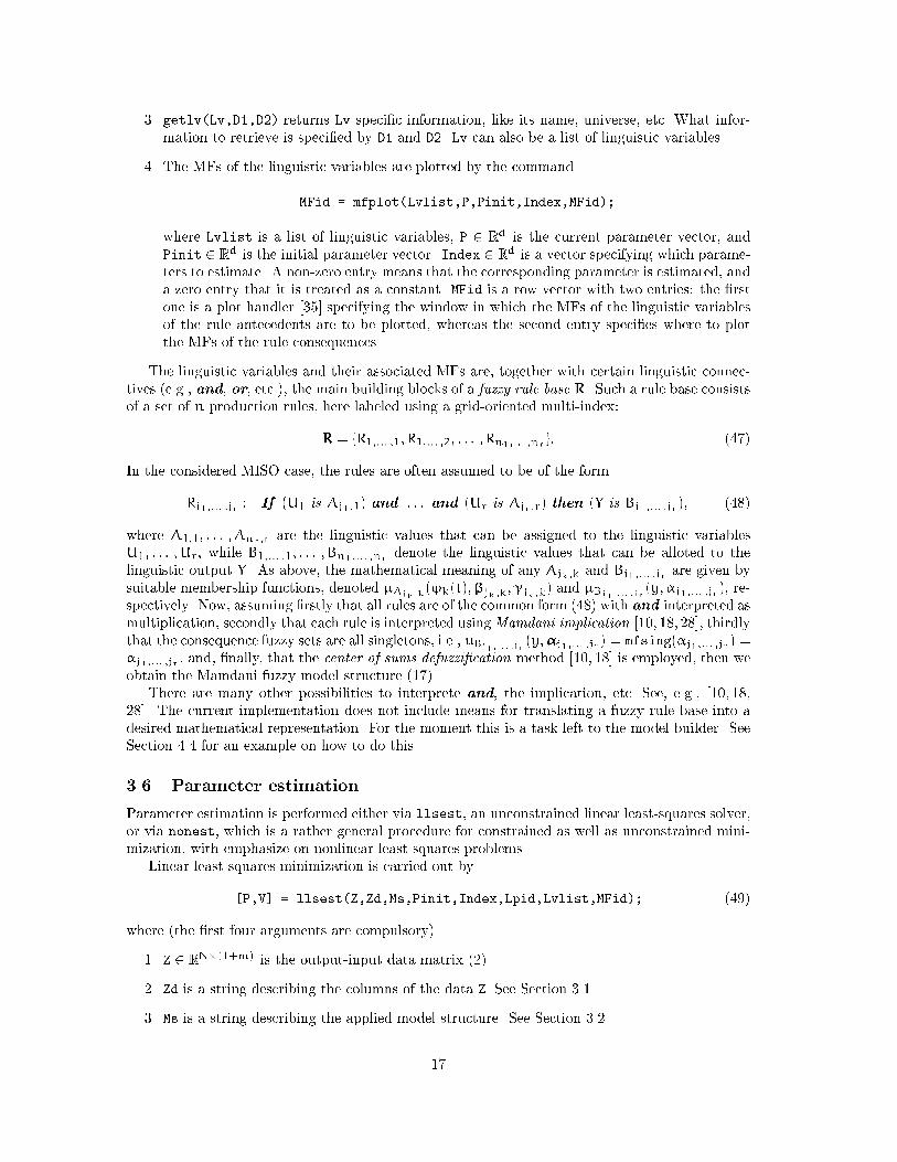
�� The MFs of the linguistic variables are plotted by the command

MFid � mfplot�Lvlist�P�Pinit�Index�MFid��

where Lvlist is a list of linguistic variables� P � Rd is the current parameter vector� and

Pinit � Rd is the initial parameter vector� Index � Rd is a vector specifying which parame�ters to estimate� A non�zero entry means that the corresponding parameter is estimated� anda zero entry that it is treated as a constant� MFid is a row vector with two entries� the �rstone is a plot handler �� specifying the window in which the MFs of the linguistic variablesof the rule antecedents are to be plotted� whereas the second entry speci�es where to plotthe MFs of the rule consequences�

The linguistic variables and their associated MFs are� together with certain linguistic connec�tives �e�g�� and� or� etc� � the main building blocks of a fuzzy rule base R� Such a rule base consistsof a set of n production rules� here labeled using a grid�oriented multi�index�

R � fR�� R�� Rn�� nrg� ��

In the considered MISO case� the rules are often assumed to be of the form

Rj�� jr � If �U� is Aj�� and � � � and �Ur is Ajr�r� then �Y is Bj�� jr��

where A�� Anr�r are the linguistic values that can be assigned to the linguistic variablesU�� Ur� while B�� Bn�� nr denote the linguistic values that can be alloted to thelinguistic output Y� As above� the mathematical meaning of any Ajk�k and Bj�� jr are given bysuitable membership functions� denoted �Ajk�k

��k�t��jk�k��jk�k� and �Bj�� jr �y� j�� jr�� re�spectively� Now� assuming �rstly that all rules are of the common form �� with and interpreted asmultiplication� secondly that each rule is interpreted usingMamdani implication �� thirdlythat the consequence fuzzy sets are all singletons� i�e�� Bj�� jr �y��j�� jr� � mfsing�j�� jr� �

j�� jr � and� �nally� that the center of sums defuzzi�cation method �� is employed� then weobtain the Mamdani fuzzy model structure �� There are many other possibilities to interprete and� the implication� etc� See� e�g��

�� The current implementation does not include means for translating a fuzzy rule base into adesired mathematical representation� For the moment this is a task left to the model builder� SeeSection �� for an example on how to do this�

�� Parameter estimation

Parameter estimation is performed either via llsest� an unconstrained linear least�squares solver�or via nonest� which is a rather general procedure for constrained as well as unconstrained mini�mization� with emphasize on nonlinear least�squares problems�Linear least�squares minimization is carried out by

�P�V � llsest�Z�Zd�Ms�Pinit�Index�Lpid�Lvlist�MFid��

where �the �rst four arguments are compulsory

� Z � RN��m� is the output�input data matrix ��

�� Zd is a string describing the columns of the data Z� See Section ��

� Ms is a string describing the applied model structure� See Section ��

�

�� Pinit � Rd is the initial parameter vector�� Index � Rd is a vector specifying what parameters to estimate� A non�zero value means thatthe corresponding parameter is estimated� and a zero value that it is left unchanged� Here itis important that only linear parameters are marked for estimation� Default� Index � �� isto estimate all the d parameters�

�� Lpid is a matlab �gure handler� The purpose of the �gure is to display how the loss �� changes throughout the estimation procedure� Default� Lpid � �� means that no plottingis performed�

�� Lvlist is a list of linguistic variables� used solely for fuzzy identi�cation purposes� SeeSection ��

�� MFid is a row vector specifying two matlab �gure handlers� one for displaying rule premiseMFs and one for displaying rule consequence MFs� Used only in conjunction with fuzzyidenti�cation� See Section ��

P � Rd is the estimated parameter vector� V is a row vector with � entries� V�� is the loss �� obtained with Pinit� and V�� theloss �� obtained with P�

Various methods for unconstrained and constrained estimation are available through

�P�V�L�Pos � nonest�Z�Zd�Ms�Pinit�Index�Con�

Ereg�Opt�Lpid�Lvlist�MFid��

where� as above� the �rst four input arguments are mandatory� while the remaining seven argumentsare optional� Of these arguments� the ones also appearing in the linear least�squares case have thesame meaning as there� The meaning and the use of the other arguments are as follows�

�� Con is a string matrix describing the constraints c�� See Section �� Constrained estima�tion using the gradient method takes place whenever Con is non�empty�

�� Ereg is a string specifying the amount of explicit regularization to impose� See Section ��The gradient method is currently the only method being able to handle this case�

�� Opt is a column vector in R�� with parameters used in the di�erent optimization routines�An empty Opt gives the default values �see below � and an Opt with fewer than elementsleads to that the remaining elements assume their default values� The elements of the Optvector are as follows�

No� Default Description

� Main optimization routine� �� Levenberg�Marquardt method �� damped Gauss�Newton method �� damped gradient method ��

� � Line search method to determine a suitable �� Halving strategy for thegradient and the Gauss�Newton methods� In the Levenberg�Marquardtcase it yields the Fletcher strategy� see page �� Marquardt�s method�applicable for the Levenberg�Marquardt procedure� see page ��

�� Maximum number of iterations performed �in the outer loop �� Maximum number of iterations performed in the inner loop� Only used

for constrained minimization�� e�� Termination criterion� Stop when jV �

N�� j is less than this value�� e�� Termination criterion� Stop when j�

�i��

N � ��i�

N j is less than this value�� Controls the amount of information sent to the screen during the opti�

mization cycle� �� display messages� �� suppress messages�� e�� Minimum allowed value of �� See Section �� e�� Maximum allowed value of �� See Section ��

�

No� Default Description

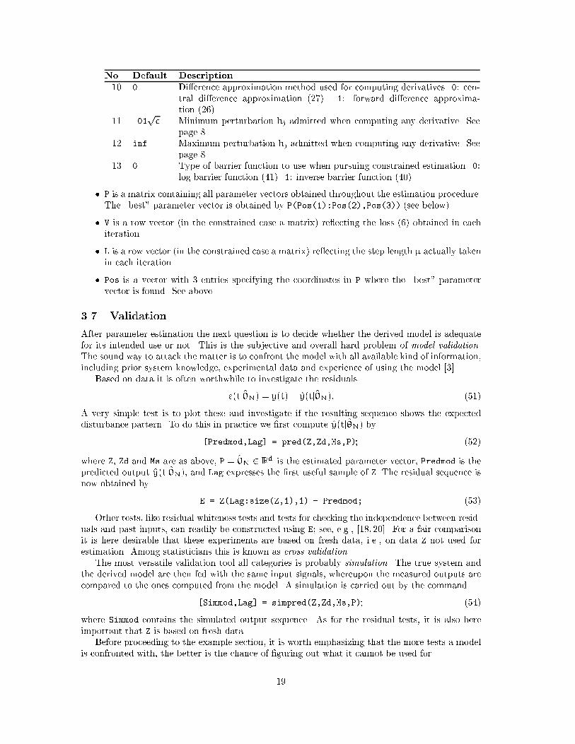
� � Di�erence approximation method used for computing derivatives� �� cen�tral di�erence approximation �� forward di�erence approxima�tion ��

��p� Minimum perturbation hj admitted when computing any derivative� See

page �� inf Maximum perturbation hj admitted when computing any derivative� See

page �� Type of barrier function to use when pursuing constrained estimation� ��

log barrier function �� inverse barrier function ��

P is a matrix containing all parameter vectors obtained throughout the estimation procedure�The �best� parameter vector is obtained by P�Pos��Pos��Pos�� see below �

V is a row vector �in the constrained case a matrix re�ecting the loss �� obtained in eachiteration�

L is a row vector �in the constrained case a matrix re�ecting the step length � actually takenin each iteration�

Pos is a vector with entries specifying the coordinates in P where the �best� parametervector is found� See above�

�� Validation

After parameter estimation the next question is to decide whether the derived model is adequatefor its intended use or not� This is the subjective and overall hard problem of model validation�The sound way to attack the matter is to confront the model with all available kind of information�including prior system knowledge� experimental data and experience of using the model ��Based on data it is often worthwhile to investigate the residuals

��tj��N� � y�t� � �y�tj��N��

A very simple test is to plot these and investigate if the resulting sequence shows the expecteddisturbance pattern� To do this in practice we �rst compute �y�tj��N� by

�Predmod�Lag � pred�Z�Zd�Ms�P� ��

where Z� Zd and Ms are as above� P � ��N � Rd is the estimated parameter vector� Predmod is thepredicted output �y�tj��N�� and Lag expresses the �rst useful sample of Z� The residual sequence isnow obtained by

E � Z�Lag�size�Z�� Predmod� ��

Other tests� like residual whiteness tests and tests for checking the independence between resid�uals and past inputs� can readily be constructed using E� see� e�g�� For a fair comparisonit is here desirable that these experiments are based on fresh data� i�e�� on data Z not used forestimation� Among statisticians this is known as cross validation�The most versatile validation tool all categories is probably simulation� The true system and

the derived model are then fed with the same input signals� whereupon the measured outputs arecompared to the ones computed from the model� A simulation is carried out by the command

�Simmod�Lag � simpred�Z�Zd�Ms�P� ��

where Simmod contains the simulated output sequence� As for the residual tests� it is also hereimportant that Z is based on fresh data�Before proceeding to the example section� it is worth emphasizing that the more tests a model

is confronted with� the better is the chance of �guring out what it cannot be used for�

�

� Application example � tank level modeling

This section illustrates the use of the software presented above� The considered system is therather simple laboratory�scale tank process shown to the left in Figure �� The identi�cation goalis to explain how the voltage u�t� �the input a�ects the water level h�t� �the output of the tank�

H � �� cm

u�t�

h�t�

�

��

� � � � � �

�

Time �min�

h�t��cm��

��

�

� � � � � �

�

Time �min�

u�t��V�

�

��

�

Figure �� Schematic picture of the laboratory�scale tank system �left�� Experimental data used forestimation �right��

Two data records each with �� output�input data pairs� one for modeling and one for vali�dation purposes� were �rst collected and then loaded into matlab by

load tankdata� �� Data file

Ze � �ye ue� �� Create estimation data See Figure �

Zv � �yv uv� �� Create validation

Zd � ��h�t��u�t�� Output�input data description

From the right plot of Figure � we notice that the measured estimation data Ze rather well coverthe interesting modeling domain�In the following sections we try four di�erent modeling approaches� simple ARX modeling�

semi�physical modeling� combined semi�physical and neural network modeling� and� �nally� fuzzymodeling� The onward discussion focuses mainly on software issues� More theoretical and furthermodeling aspects based on this application are detailed in ��

�� Simple ARX modeling

Following the �try simple things �rst� principle� a plausible �rst identi�cation attempt is to try asimple linear regression model� Experiments reveal that one of the best model structures withinthis category involves three parameters only�

�h�tj�� h�t� �� u�t � ��

which would have been a linear ARX structure if only �� was removed� This model structure isspeci�ed� the parameters are estimated using the linear least�squares scheme� and a simulation iscarried out by the commands

MsARX � �P��h�t�� P��u�t�� P�� Model structure

�PARX�VARX � llsest�Ze�Zd�MsARX�zeros�� Parameter estimation

�SimARX�Lag � simpred�Zv�Zd�MsARX�PARX�� Validation See Figure �

As can be seen to the left in Figure �� the �t between the simulated �SimARX and the measuredoutputs is quite good with the model output tracking the true output most of the time� However�

��

�

�

�

Tanklevelh�t��cm�

Measured outputsSimulated outputs

Norm of prediction errors

� � � � � �Time �min�

��

�

��

�

RMS error�Max error�

��

�

�

�




� � � � � �Time �min�

��

�

��

�


��

Figure �� Simulation behavior �based on validation data� of simple ARX �� left� and semi�physical ��right� models describing the level of the tank depicted in Figure �

the model output sequence is physically impossible since it comprises negative values� This is ofcourse a nontrivial complication if we are going to study the behavior of the real system� It shouldbe stressed that all tested simple models of the form �� show this defect� which thus motivatesother modeling approaches�

�� Semiphysical modeling

Striving to overcome the di�culty from above we next turn to some semi�physical modeling� Itis actually possible to say quite a lot about how h�t� changes as a function of the in�ow usingphysical reasoning� Let A denote the cross�sectional area of the tank� let a be the area of theoutlet hole� and� as usual� let g denote the gravitational constant� When a is small� Bernoulli�slaw states that the out�ow can be approximated by

qout�t� � ap�gph�t��

The rate of change of the amount of water in the tank at time t is equal to the in�ow qin�t�

�assumed to be proportional to u�t� minus the out�ow� i�e��

d

dt�Ah�t�� qin�t� � qout�t� � ku�t� � a

p�gph�t��

Discretizing this equation using a simple Euler approximation gives

h�t� �� h�t� �Tap�g

A

ph�t� �

Tk

Au�t��

where T is the sampling period� After reparameterization� this structure can be expressed as

�h�tj�� h�t� �� ph�t� �� u�t � ��

which is a linear regression� where the linear�least squares algorithm is applicable for parameterestimation� In terms of matlab code this situation is handled by the command sequence

Mssemi � �P��h�t�� P��sqrt�h�t�� P��u�t�� P��

�Psemi�Vsemi � llsest�Ze�Zd�Mssemi�zeros�� Parameter estimation

�Simsemi�Lag � simpred�Zv�Zd�Mssemi�Psemi�� Validation See Figure �

A simulation �Simsemi of the estimated semi�physical model is shown to the right in Figure ��The root mean square �RMS error �� of this model is as low as �� and� more importantly� nosimulated output is negative� which indicates that the model is physically sound�

�

�� Combining semiphysical and neural network modeling

Although the low�complexity semi�physical model shows such a good �t it is actually possible todo even better by combining the semi�physical model with a �small� feed�forward neural network�NN � The setup for such a blended structure� proposed in �� is depicted to the left in Figure ��Here the idea is to start o� with a semi�physical model� in this case the one obtained in

Section �� the parameter vector of this model is now denoted ��sp � The residuals

�sp�tj��sp� � h�t� � �hsp�tj��sp� ��

are then formed and used for the tuning of the neural network parameters �nn� Observe that boththe semi�physical and the neural network sub�models operate on the same regressors ��t�� This inparticular means that the purpose of the neural network is to pick up any additional dependenciesbetween the regressors and the output that could not be explained by the semi�physical model�e�g�� e�ects of whirlpools� which were clearly visible during data collection�The neural network structure �nally decided upon includes four sigmoidal activation functions�

�hnn�tj�nn� �

�Xj��

j ��Tj ��t� � �j��

��t� ��h�t� ��

ph�t� �� u�t � ��

�T� ��

where �nn � R�� so that �� parameters are estimated altogether� thereby giving the overall

predictor

�h�tj�� h�t� �� ph�t� �� u�t� ��

�Xj��

j ��Tj ��t� � �j��

Starting with the semi�physical model from Section �� the following code sequence de�nes andsolves the remaining identi�cation problem�

Znne � �Ze�� pred�Ze�Zd�Mssemi�Psemi� Ze� �� Augment the data matrix

Znnd � ��e�t��h�t��u�t�� Data used for the NN training

MsNN � ��P�� exp��P��h�t�� P��sqrt�h�t��

�P��u�t�� P��

�P�� exp��P��h�t�� P��sqrt�h�t��

�P��u�t�� P��


�P��u�t�� P��


�P��u�t�� P�� The NN model structure

PNN� � �Psemi� ��rand�� Initial parameter vector

Index � �zeros�� ones�� Estimate NN parameters only

Opt � �� Use the Levenberg�Marquardt scheme

�PNN�VNN�LNN�PosNN � nonest�Znne�Znnd�MsNN�PNN��

��Opt�� Perform parameter estimation

Mscom � �Mssemi �� MsNN� �� Define overall model structure

Pcom � PNN�PosNN��PosNN��PosNN�� Total parameter vector

�Simcom�Lag � simpred�Zv�Zd�Mscom�Pcom�� Validation See Figure �

The right plot of Figure � shows that the simulated outputs �Simcom of the combined model arevirtually impossible to distinguish from the measured ones� Furthermore� the RMS error obtainedis as low as �� which is almost half of that obtained with the semi�physical model alone�Because neural networks stand alone are good and versatile function approximators ��

an alternative to the combined approach would here be to try one single� though larger� neural

��

��t�

P�h�tj��N�h�t�

Semi�physical

modelstructure

Neuralnetworkstructure

�sp�tj��sp�

�

�

P�

�hsp�tj��sp�

�hnn�tj��nn�

�

�

�

�




� � � � � �Time �min�

��

�

��

�


��

Figure �� Right� combined two�stage semi�physical and neural network estimation procedure� Left�simulation behavior �based on validation data� of the estimated combined model of the form �� describingthe level of the tank of Figure �

network� However� we have not yet been able to obtain a physically sound model this way� Theproblems are �rstly how to �nd a reasonable size n of the model structure� and secondly how toinitialize the parameter vector to avoid getting stuck in an undesired local minimum�

�� Fuzzy modeling

A �rst problem with the above approaches is that there is no real guarantee that the modeloutputs are always physically sound for other input sequences� Secondly� even if the estimationdata set is of rather high quality it still shows some gaps� The tank is� e�g�� never emptied nor isit completely �lled up� A model structure being able to ensure such extrapolation capabilities isof course desirable� Thirdly� from simple physics we know that a certain constant input u�t� � u�

eventually leads to a �constant� liquid level h�t� � h�� Starting from such a steady�state conditionwe also know that an increase in u�t� causes h�t� to increase �in a non�oscillatory manner andsettle at a higher value� More to the point� the steady�state gain curve of a sound tank model shouldbe monotonically increasing in the input u�t� � u�� This is a non�structural system property thatwhen known is extremely important to retain in certain applications� e�g�� when the model is goingto be used in a predictive control arrangement� see �� and further references therein�It now turns out that all these features can be handled within the fuzzy framework as is shown

in �� The three linguistic variables

level�t� � fzero� very low � low � rather low � high �max g� D � �h�tj�� Y � �� cm�

level �t� �� fzero� low � highg� D � ��t� � h�t� �� U� � �� cm�

voltage�t � �� flow � highg� D � ��t� � u�t � �� U� � �� V� ��

are there used in the complete fuzzy rule base

R�� If level �t� �� is zero and voltage�t � �� is low then level�t� is zero�

R�� If level �t� �� is zero and voltage�t � �� is high then level�t� is very low �

R�� If level �t� �� is low and voltage�t� �� is low then level �t� is low �

R�� If level �t� �� is low and voltage�t� �� is high then level �t� is rather low �

R�� If level �t� �� is high and voltage�t� �� is low then level �t� is high �

R�� If level �t� �� is high and voltage�t� �� is high then level�t� is max �

��

�

The listed system properties can be guaranteed �� if the MFs

�zero��h�tj��

�very low ��h�tj��

�low ��h�tj��

�rather low ��h�tj��

�high ��h�tj��

�max ��h�tj��

and

�zero��t�� A��t�� mfl��t��

�low ��t�� A��t�� mftri��t��

�high ��t�� A��t�� mfr��t��

�low ��t�� A��t�� mfl��t��

�high ��t�� A��t�� mfr��t��

��

are used in the fuzzy predictor �the normalization factor is always for this MFs con�guration

�h�tj��

�Xj��

�Xj��

j��j�

�Yk��

�Aj��j��k�t��

which contains � free parameters

� ��

�T� ��

chosen so that

� � ��

� � ��

��

��

This modeling situation is speci�ed by the following code segment�

�� A Define linguistic variables

Lv� � ��level�t��C��cm�� Consequence ling variable

�zero � mfsing��

�very�low � mfsing�P��

�low � mfsing�P��

�rather�low � mfsing�P��

�high � mfsing�P��

�max � mfsing��

�h�t��

Lv� � ��level�t��P��cm�� Premise ling variable

�zero � mfl�u��P��

�low � mftri�u��P��

�high � mfr�u�P��

�h�t��

Lv� � ��voltage�t��P��V�� Premise ling variable

�low � mfl�u�P��P��

�high � mfr�u�P��P��

�u�t��

Lvlist � sscanf��Lv� �� Lv� �� Lv��s�� List of ling variables

�� B Specify the rules and the predictor structure

R�� mfl�h�t��P��mfl�u�t��P��P��

��

R�� P��mfl�h�t��P��mfr�u�t��P��P��

R�� P��mftri�h�t��P��mfl�u�t��P��P��

R�� P��mftri�h�t��P��mfr�u�t��P��P��

R�� P��mfr�h�t��P��mfl�u�t��P��P��

R�� mfr�h�t��P��mfr�u�t��P��P��

Msfuz � �R�� R�� R�� R�� R�� R�� Fuzzy predictor

�� C Specify intital parameters vector

Pfuz� � ��

�� D Specify parameter constraints

C� � �P�� Constraints for level�t� MFs

C� � �P�� P��

C� � �P�� P��

C� � �P�� P��

C� � � �� P��

C� � �P�� Constraints for level�t�� MFs

C� � � �� P��

C� � �P�� Constraints for voltage�t�� MFs

C� � �P�� P��

C�� P��

Con � str�mat�C��C��C��C��C��C��C��C��C��C��

It is now a straightforward matter to estimate the fuzzy parameters and evaluate the corre�sponding models�

Index � �ones�� zeros�� Estimate linear parameters only

�Pfuzl�Vfuzl � llsest�Ze�Zd�Msfuz�Pfuz��Index��

�Simfuzl�Lag � simpred�Zv�Zd�Msfuz�Pfuzl�� Validation See Figure �

Opt � �� Constrained gradient estimation

�Pfuzc�Vfuzc�Lfuzc�Posfuzc � nonest�Ze�Zd�Msfuz�Pfuzl��

Index�Con��Opt�� Perform parameter estimation

Pfuzc � Pfuzc�Posfuzc��Posfuzc��Posfuzc��

MFid � mfplot�Lvlist�Pfuzc�Pfuzl�� Plot MFs See Figure �

�Simfuzc�Lag � simpred�Zv�Zd�Msfuz�Pfuzc�� Validation See Figure �

Here� with � �xed according to the left plot of Figure � �dotted curves � the �rst unconstrainedlinear least�squares estimation of the four free centers � yields a feasible parameter estimate�see the upper right plot of Figure �� The simulation �Simfuzl detailed to the left in Figure �indicates also that this preliminary model is rather good� Starting from this point� it is now truethat unconstrained estimation �not shown of all the seven parameters �� renders a model witha lower RMS error �� compared to �� for the �rst model � but then it becomes di�cult tolinguistically interprete the obtained model� This dilemma is resolved in the code sequence aboveby constrained estimation subject to the constraints �� hence giving linguistically sound MFsas is shown in Figure � �solid curves �The simulation performance �Simfuzc of the �nal fuzzy model is shown to the right in Figure ��

The RMS error of this model �� is quite low� yet not as low as is obtained with the combinedmodel of Section �� However� contrary to that case� it is here possible to guarantee certainextrapolation and steady�state gain monotonicity features� which for some applications are moreimportant than just applying the model with lowest RMS error�

��

U� �V�

�

zero

�

��

��

��

�

� � �

U� �cm��

low

high

low

high

voltage�t��

level�t��

� �

Y �V�

�

zero

�

Y �V��

max

zero

max

level�t�

level�t�

� �

��

� ��

verylow

low

ratherlow

high

��

verylow

low

ratherlow

high

Figure � Premise �left� and consequence �right� MFs for describing the liquid level of the tank system�Dotted curves show the situation when only the centers � are estimated� Solid curves show the situationafter constrained estimation subject to the constraints ��

�

�

�




� � � � � �Time �min�

��

�

��

�


��

�

�

�




� � � � � �Time �min�

��

�

��

�


��

Figure � Simulation �based on validation data� of unconstrained linear least�squares �left� and con�strained �right� estimated fuzzy models of the form �� re�ecting the liquid level of the tank of Figure �

� Conclusions and extensions

In this paper we have discussed a number of system identi�cation algorithms and how to imple�ment them� Based on these algorithms� we then described the use of a prototype identi�cationsoftware tool� applicable for the class of MISO model structures with regressors that are formedby delayed in� and outputs only� The usefulness and the versatility of the developed softwarewere demonstrated on experimental data from a simple tank system� which was modeled by fourdi�erent approaches� simple ARX modeling� semi�physical modeling� combined semi�physical andneural network modeling� and� �nally� fuzzy modeling�The software employed for these experiments consists of a number of matlab m��les� which

can be downloaded from the library

ftp��ftpcontrolisyliuse�pub�Software�Fuzzy�

To this end� let us �nally point to some possible and nice�to�have extensions of this package�

� Concerning numeric algorithms further e�orts should be put into data pre�processing andvalidation methods�

Another activity already being initiated is the implementation of some more estimation pro�cedures� We are here planning to include a conjugate gradient method �� to directly arrive

��

at a Newton search direction without having to explicitly form and invert the Hessian �� We are also planning to incorporate a constrained linear least�squares procedure �� as wellas a more e�cient algorithm for the constrained nonlinear least�squares case ��

A third numeric issue is to handle MIMO systems and to allow model structures that involvepredicted and�or simulated outputs�

�� Of the other services shown in Figure � the most urgent need is perhaps a graphical userinterface relieving the user from the burdensome and error prone task of textually enteringmodel structures� constraints� etc� Even if matlab supports GUI means the design andimplementation of such an identi�cation supervisor is likely to be quite time�consuming�

Acknowledgments

This work was supported by the Swedish Research Council for Engineering Sciences �TFR � whichis gratefully acknowledged�

References

�� S� A� Billings� Identi�cation of nonlinear systems a survey� IEE Proceedings� ��

�� !A� Bj"ork� Numerical Methods for Least Squares Problems� SIAM� ��

�� T� Bohlin� Grey�box identi�cation� a case study� Technical Report TRITA�REG�� De�partment of Automatic Control� Royal Institute of Technology� Stockholm� Sweden� ��

�� L� Breiman� Hinging hyperplanes for regression� classi�cation� and function approximation�IEEE Transactions on Information Theory� �� May ��

�� L� Breiman� J� H� Friedman� R� A� Olshen� and C� J� Stone� Classi�cation and Regression

Trees� The Wadsworth Statistics�Probability Series� Wadsworth # Brooks� ��

�� D� Chen and C� Moler� Symbolic Math Toolbox� The MathWorks� Inc�� Cochituate Place�Natick� MA� USA� ��

�� S� Chen and S� A� Billings� Neural networks for nonlinear dynamic system modelling andidenti�cation� International Journal of Control� ��

�� H� Demuth and M� Beale� Neural Network Toolbox� The MathWorks� Inc�� Cochituate Place�Natick� MA� USA� ��

�� J� E� Dennis and R� B� Schnabel� Numerical Methods for Unconstrained Optimization and

Nonlinear Equations� Prentice Hall� ��

�� D� Driankov� H� Hellendoorn� and M� Reinfrank� An Introduction to Fuzzy Control� Springer�Verlag� ��

�� R� Fletcher� Practical Methods of Optimization� John Wiley # Sons� ��

�� U� Forssell and P� Lindskog� Combining semi�physical and neural network modeling� an exam�ple of its usefulness� �� Submitted to the th IFAC Symposium on System Identi�cation�SYSID�� to be held in Fukuoka� Japan� July ��

�� G� H� Golub and C� F� Van Loan� Matrix Computations� Johns Hopkins University Press��nd edition� ��

��

�� A� Grace� Optimization Toolbox� The MathWorks� Inc�� Cochituate Place� Natick� MA� USA��

�� S� Haykin� Neural Networks� A Comprehensive Foundation� Macmillan� ��

�� S� Y� Kung� Digital Neural Networks� Prentice Hall� ��

�� C��T� Lin and C� S� G� Lee� Neural Fuzzy Systems� A Neuro�Fuzzy Synergism to Intelligent

Systems� Prentice Hall� ��

�� P� Lindskog� Methods� Algorithms and Tools for System Identi�cation Based on Prior Knowl�

edge� Phd thesis �� Department of Electrical Engineering� Link"oping University� Link"oping�Sweden� May ��

�� P� Lindskog and L� Ljung� Tools for semiphysical modelling� International Journal of Adap�tive Control and Signal Processing� �� November�December �� Identi�cation�nonlinear systems�

�� L� Ljung� System Identi�cation� Theory for the User� Prentice Hall� ��

�� L� Ljung� System Identi�cation Toolbox� The MathWorks� Inc�� Cochituate Place� Natick�MA� USA� ��

�� L� Ljung� J� Sj"oberg� and H� Hjalmarsson� On neural network model structures in systemidenti�cation� In S� Bittanti and G� Picci� editors� Identi�cation� Adaptation� Learning� TheScience of Learning Models from Data� volume � of Series F� Computer and Systems Sci�

ences� pages �� Springer�Verlag� ��

�� P� Nagy� Tools for Knowledge�Based Signal Processing with Applications to System Identi�ca�

tion� Phd thesis �� Department of Electrical Engineering� Link"oping University� Link"oping�Sweden� June ��

�� T� Poggio and F� Girosi� Networks for approximation and learning� Proceedings of the IEEE��

�� P� Pucar and J� Sj"oberg� On the hinge �nding algorithm for hinging hyperplanes � revisedversion� Technical Report LiTH�ISY�R�� Department of Electrical Engineering� Link"opingUniversity� Link"oping� Sweden� �� Available by anonymous ftp ��

�� P� Pucar and J� Sj"oberg� Parameterization and conditioning of hinging hyperplane models�Technical Report LiTH�ISY�R�� Department of Electrical Engineering� Link"oping Uni�versity� Link"oping� Sweden� �� Available by anonymous ftp ��

�� J��S� Roger Jang and N� Gulley� Fuzzy Logic Toolbox� The MathWorks� Inc�� CochituatePlace� Natick� MA� USA� ��

�� J��S� Roger Jang and C��T� Sun� Neuro�fuzzy modeling and control� Proceedings of the IEEE�� March ��

�� L� E� Scales� Introduction to Non�linear Optimization� Computer Science Series� Macmillan��

�� J� Sj"oberg� Q� Zhang� L� Ljung� A� Benveniste� B� Delyon� P��Y� Glorennec� H� Hjalmarsson�and A� Juditsky� Nonlinear black�box modeling in system identi�cation� a uni�ed overview�Automatica� �� December ��

�� T� S"oderstr"om and P� Stoica� System Identi�cation� Prentice Hall International� ��

��

�� J� A� S$rlie� On Grey Box Model De�nition and Symbolic Derivation of Extended Kalman

Filters� Phd thesis TRITA�REG�� Department of Signals� Sensors and Systems� RoyalInstitute of Technology� Stockholm� Sweden� June ��

�� J��E� Str"omberg� F� Gustafsson� and L� Ljung� Trees as black�box model structures for dy�namical systems� Technical Report LiTH�ISY�I�� Department of Electrical Engineering�Link"oping University� Link"oping� Sweden� ��

�� T� Takagi and M� Sugeno� Fuzzy identi�cation of systems and its applications to modelingand control� IEEE Transactions on Systems� Man� and Cybernetics� SMC�� January�February ��

�� The MathWorks� Inc�� Cochituate Place� Natick� MA� USA� MATLAB� High�Performance

Numeric Computation and Visualization Software� ��

�� B� Wahlberg� System identi�cation using Laguerre models� IEEE Transactions on Automatic

Control� AC�� May ��

�� B� Wahlberg� System identi�cation using Kautz models� IEEE Transactions on Automatic

Control� AC�� June ��

�� G� Watson� Smooth regression analysis� Sankhya� Series� A��

�� Q� Zhang and A� Benveniste� Wavelet networks� IEEE Transactions on Neural Networks��

��

Documents

System - DiVA portal