SYSTEM DESIGN AND PERFORMANCE COMPARISON OF BLENDED

GASOLINE/ETHANOL FUELS IN SEMI-DIRECT AND DIRECT INJECTED

TWO-STROKE ENGINES

A Thesis

Presented in Partial Fulfillment of the Requirements for the

Degree of Master of Science

with a

Major in Mechanical Engineering

in the

College of Graduate Studies

University of Idaho

by

Nicholas J. Harker

May 2009

Major Professor: Karen DenBraven, Ph.D.

ii

AUTHORIZATION TO SUBMIT THESIS

This thesis of Nicholas J. Harker, submitted for the degree of Master of Science with a

major in Mechanical Engineering and titled “System Design and Performance

Comparison of Blended Gasoline/Ethanol Fuels in Semi-Direct and Direct Injected Two-

Stroke Engines,” has been reviewed in final form. Permission, as indicated by the

signatures and dates given below, is now granted to submit final copies to the College of

Graduate Studies for approval.

Major Professor ________________________________ Date ________

Karen DenBraven, Ph.D.

Committee

Member ________________________________ Date ________

Steven Beyerlein, Ph.D.

Committee

Member ________________________________ Date ________

David Egolf, Ph.D.

Department

Administrator ________________________________ Date ________

Karen DenBraven, Ph.D.

Discipline’s

College Dean ________________________________ Date ________

Donald Blackketter, Ph.D.

Final Approval and Acceptance by the College of Graduate Studies

________________________________ Date _______

Margrit von Braun

iii

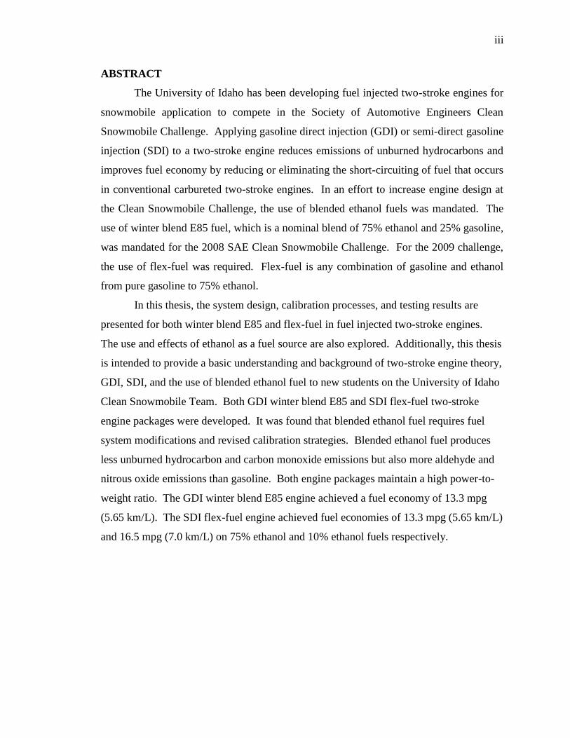
ABSTRACT

The University of Idaho has been developing fuel injected two-stroke engines for

snowmobile application to compete in the Society of Automotive Engineers Clean

Snowmobile Challenge. Applying gasoline direct injection (GDI) or semi-direct gasoline

injection (SDI) to a two-stroke engine reduces emissions of unburned hydrocarbons and

improves fuel economy by reducing or eliminating the short-circuiting of fuel that occurs

in conventional carbureted two-stroke engines. In an effort to increase engine design at

the Clean Snowmobile Challenge, the use of blended ethanol fuels was mandated. The

use of winter blend E85 fuel, which is a nominal blend of 75% ethanol and 25% gasoline,

was mandated for the 2008 SAE Clean Snowmobile Challenge. For the 2009 challenge,

the use of flex-fuel was required. Flex-fuel is any combination of gasoline and ethanol

from pure gasoline to 75% ethanol.

In this thesis, the system design, calibration processes, and testing results are

presented for both winter blend E85 and flex-fuel in fuel injected two-stroke engines.

The use and effects of ethanol as a fuel source are also explored. Additionally, this thesis

is intended to provide a basic understanding and background of two-stroke engine theory,

GDI, SDI, and the use of blended ethanol fuel to new students on the University of Idaho

Clean Snowmobile Team. Both GDI winter blend E85 and SDI flex-fuel two-stroke

engine packages were developed. It was found that blended ethanol fuel requires fuel

system modifications and revised calibration strategies. Blended ethanol fuel produces

less unburned hydrocarbon and carbon monoxide emissions but also more aldehyde and

nitrous oxide emissions than gasoline. Both engine packages maintain a high power-to-

weight ratio. The GDI winter blend E85 engine achieved a fuel economy of 13.3 mpg

(5.65 km/L). The SDI flex-fuel engine achieved fuel economies of 13.3 mpg (5.65 km/L)

and 16.5 mpg (7.0 km/L) on 75% ethanol and 10% ethanol fuels respectively.

iv

ACKNOWLEDGEMENTS

This work was made possible through funding and support from the National

Institute for Advanced Transportation Technology (NIATT). My major professor, Dr.

Karen DenBraven, deserves thanks for her guidance on this thesis and for her time and

devotion to the University of Idaho Clean Snowmobile Team. My committee members,

Dr. Steven Beyerlein and Dr. David Egolf, also deserve thanks for their help in reviewing

this thesis. Dylan Dixon, Alex Fuhrman, Peter Britanyak, Justin Johnson, the 2008 and

2009 University of Idaho Clean Snowmobile Teams, Andrew Findlay, Dan Nehmer, Dan

Cordon, Russ Porter, and the E-lab deserve a big thanks for their support and numerous

hours of bench-racing. I would also like to thank Chris Harker, Dena Harker, and Caitlin

Flynn for their support and understanding during my time at the University of Idaho.

v

TABLE OF CONTENTS

AUTHORIZATION TO SUBMIT THESIS ................................................................... ii

ABSTRACT ...................................................................................................................... iii

ACKNOWLEDGEMENTS ............................................................................................ iv

LIST OF FIGURES ........................................................................................................ vii

LIST OF TABLES ......................................................................................................... viii

DEFINITION OF TERMS.............................................................................................. ix

1.0 INTRODUCTION.................................................................................................. 1

1.1 THESIS GOALS .................................................................................................. 2

1.2 SAE CLEAN SNOWMOBILE CHALLENGE ................................................... 2

1.3 UNIVERSITY OF IDAHO’S CSC HISTORY ................................................... 4

2.0 THE TWO-STROKE ENGINE ........................................................................... 6

2.1 ENGINE SELECTION ........................................................................................ 6

2.2 TWO-STROKE ENGINE FUEL INJECTION.................................................... 7

2.2.1 Semi-Direct Fuel Injection ....................................................................................... 8

2.2.2 Gasoline Direct Injection ......................................................................................... 9

2.2.3 University of Idaho GDI System Design ................................................................ 11

2.2.4 University of Idaho GDI Cylinder Head Design .................................................... 12

3.0 BLENDED ETHANOL FUELS ......................................................................... 16

3.1 ENVIRONMENTAL IMPACTS OF BLENDED ETHANOL FUELS ............ 16

3.2 PROPERTIES OF BLENDED ETHANOL FUELS ......................................... 18

3.3 ENGINE SYSTEM DESIGN FOR BLENDED ETHANOL FUELS ............... 21

4.0 UNIVERSTIY OF IDAHO ENGINE SYSTEM DESIGN ............................... 23

4.1 FUEL INJECTION SELECTION ...................................................................... 23

4.2 FUEL SYSTEM ................................................................................................. 24

4.3 FLEX-FUEL SYSTEM ...................................................................................... 24

vi

4.4 CALIBRATION STRATEGIES ........................................................................ 25

4.4.1 Winter Blend E85 GDI Two-Stroke Engine ........................................................... 26

4.4.2 Flex-Fuel SDI Two-Stroke Engine ......................................................................... 27

5.0 TESTING .............................................................................................................. 29

5.1 METHODOLOGY ............................................................................................. 29

5.1.1 Brake Specific Fuel Consumption .......................................................................... 29

5.1.2 Lambda .................................................................................................................. 30

5.1.3 Fuel Economy ........................................................................................................ 31

5.2 TESTING EQUIPMENT ................................................................................... 32

5.2.1 Water-Brake Dynamometer ................................................................................... 32

5.2.2 Eddy Current Dynamometer .................................................................................. 34

5.2.3 Wideband Lambda Meter ....................................................................................... 38

5.2.4 Fuel Measurement ................................................................................................. 39

6.0 RESULTS AND CONCLUSIONS ..................................................................... 40

6.1 E85 GASOLINE DIRECT INJECTION............................................................ 40

6.2 FLEX-FUEL SEMI-DIRECT INJECTION ....................................................... 44

6.3 FUEL INJECTION ............................................................................................ 46

6.4 CONCLUSIONS ................................................................................................ 47

7.0 RECOMMENDATIONS AND FUTURE WORK ........................................... 49

7.1 INCREASED/VARIABLE COMPRESSION ................................................... 49

7.2 HIGH-PRESSURE DIRECT INJECTION ........................................................ 49

7.3 CHARGE TRAPPING ....................................................................................... 50

7.4 TESTING EQUIPMENT ................................................................................... 51

BIBLIOGRAPHY ........................................................................................................... 52

APPENDIX A – BRAKE SPECIFIC FUEL CONSUMPTION OPTIMIZATION . 56

vii

LIST OF FIGURES

Figure 1: Possible SDI cylinder geometry ........................................................................ 8

Figure 2: The Lambda and Charge Stratification for Stratified and Homogeneous

Combustion ....................................................................................................................... 10

Figure 3: Cross-Section of the E-TEC injector ............................................................... 12

Figure 4: Loop-Scavenged GDI Engine Fuel-Spray Targeting Strategies ..................... 13

Figure 5: Cross Section of the University of Idaho GDI Combustion Chamber ............. 14

Figure 6: The University of Idaho GDI Cylinder Head .................................................. 15

Figure 7: Reid Vapor Pressure of Blended Ethanol Fuel................................................ 17

Figure 8: Flex-Fuel Sensor ............................................................................................. 22

Figure 9: Flex-Fuel Sensor Output Calibration .............................................................. 25

Figure 10: Flex-Fuel LED Ethanol Content Display ...................................................... 25

Figure 11: Land and Sea DYNOmite™ Dynamometer Head ....................................... 32

Figure 12: Torque and Power Ratings of the Dynamometer Head................................. 33

Figure 13: Power and Torque Ratings of the FE-260-S Dynamometer .......................... 34

Figure 14: Eddy Current Dynamometer Strain Gauge ................................................... 35

Figure 15: Eddy Current Dynamometer and Test Engine .............................................. 36

Figure 16: Dynamometer Wireless Handheld Controller ............................................... 37

Figure 17: Dynamometer Control System/Sensor Interface ........................................... 37

Figure 18: Eddy Current Dynamometer Testing Diagram ............................................. 38

Figure 19: Wideband Lambda Meter and Oxygen Sensor ............................................. 38

Figure 20: Fuel Conditioning/Metering and Display Units ............................................ 39

Figure 21: Rated Power Output Comparison between E10 and E75 .............................. 42

Figure 22: Average Modal BSFC Comparison between E10 and E75........................... 42

Figure 23: Flex-Fuel Injection Quantity Compensation Map ......................................... 45

Figure 24: Average Modal Flex-Fuel BSFC Comparison .............................................. 46

Figure 25: GDI and SDI Fuel System BSFC Comparison ............................................. 47

Figure 26: Charge Trapping Stages: Blow-Down, Intake, and Trapping/Compression . 50

viii

LIST OF TABLES

Table 1: Weighted Five-Mode Testing Points for a Snowmobile Engine ........................ 3

Table 2: Maximum Emission Levels for EPA and NPS Standards .................................. 4

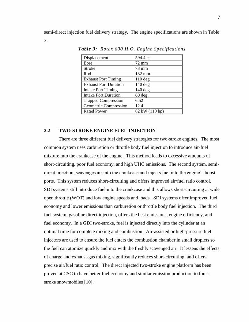
Table 3: Rotax 600 H.O. Engine Specifications ............................................................... 7

Table 4: Five-Mode Emissions and Fuel Economy of Two and Four-Stroke CSC

Control Snowmobiles.......................................................................................................... 9

Table 5: Properties of Gasoline and Ethanol .................................................................. 16

Table 6: Ethanol Sensitive and Non-Compatible Materials............................................ 20

Table 7: Typical 25-45 mph (40-73 km/hr) Cruise Points of the Rotax 600cc Engine .. 30

Table 8: E10 Injection Quantity (mm3)........................................................................... 40

Table 9: Winter Blend E85 Injection Quantity (mm3) .................................................... 41

ix

DEFINITION OF TERMS

AFR: Air-Fuel Ratio

AFRS: Stoichiometric Air-Fuel Ratio

AKI: Anti-Knock Index

BSFC: Brake Specific Fuel Consumption

BTDC: Before Top Dead Center

CO: Carbon Monoxide

CFD: Computational Fluid Dynamics

CSC: Clean Snowmobile Challenge

CVT: Continuously Variable Transmission

E: EPA Emission Number

E0: 100% Gasoline/0% Ethanol Fuel Blend

E10: 90% Gasoline/10% Ethanol Fuel Blend

E75: 25% Gasoline/75% Ethanol Fuel Blend

E85: 15% Gasoline/85% Ethanol Fuel Blend

ECU: Engine Control Unit

EFI: Electronic Fuel Injection

EPA: Environmental Protection Agency

GDI: Gasoline Direct Injection

HPDI: High-Pressure Direct Injection

LHV: Lower Heating Value

MON: Motor Octane Number

NOx: Nitrogen Oxides

NPS: National Park Service

O3: Ozone

PAN: Peroxylacetate Nitrate

ppm: Parts Per Million

RON: Research Octane Number

RSS: Root Sum Square

RVP: Reid Vapor Pressure

SAE: Society of Automotive Engineers

x

SDI: Semi-Direct Gasoline Injection

SwRI: Southwest Research Institute

TDC: Top Dead Center

UHC: Unburned Hydrocarbons

WOT: Wide Open Throttle

1

1.0 INTRODUCTION

Increased environmental concern and reduced oil supplies have led to the

exploration of new engine technologies and the use of renewable fuels. In the United

States, corn ethanol blended with gasoline is becoming prevalent. This is because

blended ethanol fuels are agriculturally renewable and reduce dependency on foreign oil

[1]. Currently, blended ethanol fuels are primarily used in on-road transportation

vehicles, but increasing use and availability has lead to the investigation of its use in

recreational vehicles.

To address environmental concerns, there have been extensive improvements in

engine technology used in recreational vehicles. Semi-direct gasoline injection (SDI) and

gasoline direct injection (GDI) are developments that have seen much activity in the past

few years. SDI systems inject fuel into the boost port of the engine, thereby improving

fuel economy and reducing emissions. Typical GDI systems inject fuel directly in to the

combustion chamber, offering precise fuel control, reduced short-circuiting, and allowing

for different modes of combustion. When applied to the two-stroke engine, GDI can

offer large reductions in unburned hydrocarbon emissions and greatly improved fuel

efficiency.

Since 2003, the University of Idaho has been developing GDI for use in a two-

stroke snowmobile engine. This work is part of an ongoing student design project for the

Society of Automotive Engineers (SAE) Clean Snowmobile Challenge (CSC). In an

effort to increase engine design at the competition, the use of blended ethanol fuels has

recently been mandated by the competition. The use of winter blend E85 fuel, which is a

nominal blend of 75% ethanol and 25% gasoline, was mandated by the 2008 SAE Clean

Snowmobile Challenge. Prior to the 2008 CSC, the use of E10 (10% ethanol /90%

gasoline) was allowed for fueled engines with the option of using winter blend E85. For

the 2009 challenge, the use of flex-fuel was required. Flex-fuel is any combination of

gasoline and ethanol from pure gasoline to 75% ethanol. The research presented in this

thesis deals with the engine conversions and calibration necessary to efficiently run a fuel

injected two-stroke engine on both winter blend E85 and flex-fuel.

The characteristics and combustion properties of blended ethanol fuels are

significantly different than those of pure gasoline fuels. This leads to necessary engine

2

modifications and different calibration strategies. These modifications are discussed with

respect to both SDI and GDI two-stroke engines. Due to the way fuel is introduced into

the cylinders of GDI and SDI engines, modifications for ethanol are different than those

required for traditional fuel injected engines.

1.1 THESIS GOALS

The necessary engine modifications and calibration strategies to efficiently

combust blended ethanol fuels in fuel injected two-stroke engines is the primary focus of

this work. To provide background for the University of Idaho CSC team and set a

baseline for comparison, the engine setup, calibration, and results will be explored for

fuel injected two-stroke engines running on gasoline, winter blend E85, and flex-fuel.

Engine characteristics such as power output and engine efficiency will be compared for

the different fuels. A secondary goal is to explore the use and effects of ethanol as a fuel

source.

1.2 SAE CLEAN SNOWMOBILE CHALLENGE

The Clean Snowmobile Challenge was started in 2000 in an attempt to promote

the development of clean and quiet snowmobiles [2]. The goal of the competition is to

reduce unburned hydrocarbon (UHC) and carbon monoxide (CO) emissions without

increasing nitrogen oxides (NOX) emissions and reduce noise output while maintaining or

improving factory power output and handling characteristics. The CSC event targets the

problem of operating snowmobiles in environmentally sensitive areas such as

Yellowstone National Park [2].

Currently, there are two emissions standards for snowmobiles: the 2012

Environmental Protection Agency (EPA) standards and the National Park Service (NPS)

standards. The 2012 EPA standards must be met as a corporate average by all

snowmobile manufacturers by 2012. The NPS standards are stricter than the EPA

standards and are required for a snowmobile to operate in Yellowstone National Park,

Grand Teton National Park, or Rockefeller Memorial Park [3]. To determine whether a

snowmobile meets the EPA or NPS standards, a weighted five mode test developed by

the Southwest Research Institute (SwRI) is performed on the engine, which represents the

duty cycle for snowmobile engines while in operation [4]. During the test, emissions

3

measurements are taken at five combinations of engine speed and power outputs, with

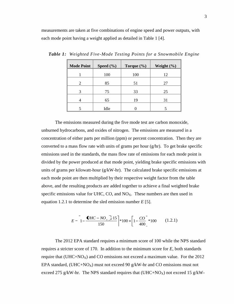
each mode point having a weight applied as detailed in Table 1 [4].

Table 1: Weighted Five-Mode Testing Points for a Snowmobile Engine

Mode Point Speed (%) Torque (%) Weight (%)

1 100 100 12

2 85 51 27

3 75 33 25

4 65 19 31

5 Idle 0 5

The emissions measured during the five mode test are carbon monoxide,

unburned hydrocarbons, and oxides of nitrogen. The emissions are measured in a

concentration of either parts per million (ppm) or percent concentration. Then they are

converted to a mass flow rate with units of grams per hour (g/hr). To get brake specific

emissions used in the standards, the mass flow rate of emissions for each mode point is

divided by the power produced at that mode point, yielding brake specific emissions with

units of grams per kilowatt-hour (g/kW-hr). The calculated brake specific emissions at

each mode point are then multiplied by their respective weight factor from the table

above, and the resulting products are added together to achieve a final weighted brake

specific emissions value for UHC, CO, and NOX. These numbers are then used in

equation 1.2.1 to determine the sled emission number E [5].

100*400

1100*150

151

CONOUHCE x (1.2.1)

The 2012 EPA standard requires a minimum score of 100 while the NPS standard

requires a stricter score of 170. In addition to the minimum score for E, both standards

require that (UHC+NOX) and CO emissions not exceed a maximum value. For the 2012

EPA standard, (UHC+NOX) must not exceed 90 g/kW-hr and CO emissions must not

exceed 275 g/kW-hr. The NPS standard requires that (UHC+NOX) not exceed 15 g/kW-

4

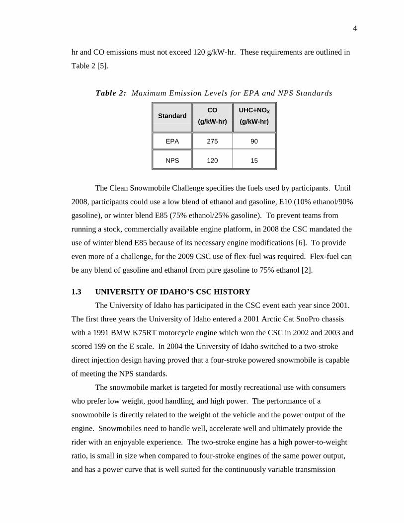
hr and CO emissions must not exceed 120 g/kW-hr. These requirements are outlined in

Table 2 [5].

Table 2: Maximum Emission Levels for EPA and NPS Standards

Standard CO

(g/kW-hr)

UHC+NOX

(g/kW-hr)

EPA 275 90

NPS 120 15

The Clean Snowmobile Challenge specifies the fuels used by participants. Until

2008, participants could use a low blend of ethanol and gasoline, E10 (10% ethanol/90%

gasoline), or winter blend E85 (75% ethanol/25% gasoline). To prevent teams from

running a stock, commercially available engine platform, in 2008 the CSC mandated the

use of winter blend E85 because of its necessary engine modifications [6]. To provide

even more of a challenge, for the 2009 CSC use of flex-fuel was required. Flex-fuel can

be any blend of gasoline and ethanol from pure gasoline to 75% ethanol [2].

1.3 UNIVERSITY OF IDAHO’S CSC HISTORY

The University of Idaho has participated in the CSC event each year since 2001.

The first three years the University of Idaho entered a 2001 Arctic Cat SnoPro chassis

with a 1991 BMW K75RT motorcycle engine which won the CSC in 2002 and 2003 and

scored 199 on the E scale. In 2004 the University of Idaho switched to a two-stroke

direct injection design having proved that a four-stroke powered snowmobile is capable

of meeting the NPS standards.

The snowmobile market is targeted for mostly recreational use with consumers

who prefer low weight, good handling, and high power. The performance of a

snowmobile is directly related to the weight of the vehicle and the power output of the

engine. Snowmobiles need to handle well, accelerate well and ultimately provide the

rider with an enjoyable experience. The two-stroke engine has a high power-to-weight

ratio, is small in size when compared to four-stroke engines of the same power output,

and has a power curve that is well suited for the continuously variable transmission

5

(CVT) type drive train found in snowmobiles. However, the two-stroke engine has

historically suffered from poor fuel economy and high levels of UHC emissions. Due to

increasing environmental concerns, stricter emissions regulations are affecting the

recreational vehicle market, forcing manufacturers to develop cleaner engine

technologies. This often means using a four-stroke engine in place of a two-stroke for the

benefit of decreased emissions and improved fuel economy. This solution path has been

proven time and again through the SAE CSC. From 2000-2006 all CSC winners were

powered by four-stroke engines with catalytic converter aftertreatment. The University

of Idaho won two of these years by retrofitting a four-stroke motorcycle engine into a

snowmobile chassis. However, these modifications sacrificed power and increased

weight over a similar two-stroke design.

With the recent improvements to fuel delivery systems, specifically direct

injection, the potential for improved emissions and fuel economy in two-stroke engines

are greatly enhanced. Evinrude outboard engines have reliably and repeatedly proven

that GDI two-stroke engine technology is capable of emissions levels equivalent to those

of four-stroke engines [7]. With these data, the University of Idaho decided to take on

the challenge of implementing direct injection to a two-stroke snowmobile engine for the

CSC in an attempt to meet the 2012 EPA standard and to eventually the NPS standard

without sacrificing the high power output and low weight that are preferred by the

majority of snowmobile riders [8,9]. In 2007, the University of Idaho placed first at the

CSC using a GDI two-stroke engine platform. Along with first place, the University of

Idaho was also awarded best handling, best ride, best performance, best fuel economy at

19.6 mpg, lightest snowmobile, and passed the 2012 EPA emission standard [10].

6

2.0 THE TWO-STROKE ENGINE

The two-stroke engine is a low maintenance, high power-to-weight ratio internal

combustion engine. The high power density of the two-stroke engine lends itself well to

recreational applications such as snowmobiles and motorcycles. Snowmobile

applications also benefit from the two-stroke engine’s ability to reliably cold start down

to -40°C (-40°F) [11]. Two-stroke engines are much simpler than four-stroke engines, as

the only moving components are the piston, connecting rod, and crankshaft. There is no

valve train in a two-stroke engine; air-flow is controlled by ports in the cylinder wall and

the piston location. Four-stroke engines must power the valve train to regulate intake and

exhaust flows. Utilizing cylinder ports, the two-stroke engine has a combustion event

every other stroke or every crankshaft revolution. In one crankshaft revolution the two-

stroke engine intakes fresh charge, compresses the mixture, burns the compressed

mixture, and exhausts the combustion products. Four-stroke engines require two

revolutions of the crankshaft to complete the same process. For a more complete

discussion of the two-stroke engine cycle see Justin Johnson’s thesis [12].

While the design of a two-stroke engine allows for a higher power density than a

four-stroke, it also traditionally produces more hazardous emissions. The four-stroke

engine mechanically separates the intake, combustion, and exhaust processes, while the

two-stroke relies on fluid flows and acoustics. This traditionally meant poor fuel

economy and elevated hazardous emission levels. Recently, technology has allowed for

two-stroke engines to retain their high power-to-weight ratio, meet current emission

standards, and obtain similar if not better fuel efficiency than four-stroke engines. This

advanced two-stroke technology will be discussed in later sections.

2.1 ENGINE SELECTION

The University of Idaho CSC team selected a Rotax 600 H.O. two-stroke engine

for modification. This engine is widely used in the snowmobile industry as it is found in

many Ski-Doo snowmobile models. It also meets the CSC competition maximum

displacement limit of 600cc for two-stroke engines [2]. The Rotax engine is best

classified as a reed valved, crankcase charged, and Schnürle loop scavenged two-stroke

with variable exhaust and a tuned exhaust pipe. Typically, it is uses either a carbureted or

7

semi-direct injection fuel delivery strategy. The engine specifications are shown in Table

3.

Table 3: Rotax 600 H.O. Engine Specifications

Displacement 594.4 cc

Bore 72 mm

Stroke 73 mm

Rod 132 mm

Exhaust Port Timing 110 deg

Exhaust Port Duration 140 deg

Intake Port Timing 140 deg

Intake Port Duration 80 deg

Trapped Compression 6.52

Geometric Compression 12.4

Rated Power 82 kW (110 hp)

2.2 TWO-STROKE ENGINE FUEL INJECTION

There are three different fuel delivery strategies for two-stroke engines. The most

common system uses carburetion or throttle body fuel injection to introduce air-fuel

mixture into the crankcase of the engine. This method leads to excessive amounts of

short-circuiting, poor fuel economy, and high UHC emissions. The second system, semi-

direct injection, scavenges air into the crankcase and injects fuel into the engine’s boost

ports. This system reduces short-circuiting and offers improved air/fuel ratio control.

SDI systems still introduce fuel into the crankcase and this allows short-circuiting at wide

open throttle (WOT) and low engine speeds and loads. SDI systems offer improved fuel

economy and lower emissions than carburetion or throttle body fuel injection. The third

fuel system, gasoline direct injection, offers the best emissions, engine efficiency, and

fuel economy. In a GDI two-stroke, fuel is injected directly into the cylinder at an

optimal time for complete mixing and combustion. Air-assisted or high-pressure fuel

injectors are used to ensure the fuel enters the combustion chamber in small droplets so

the fuel can atomize quickly and mix with the freshly scavenged air. It lessens the effects

of charge and exhaust-gas mixing, significantly reduces short-circuiting, and offers

precise air/fuel ratio control. The direct injected two-stroke engine platform has been

proven at CSC to have better fuel economy and similar emission production to four-

stroke snowmobiles [10].

8

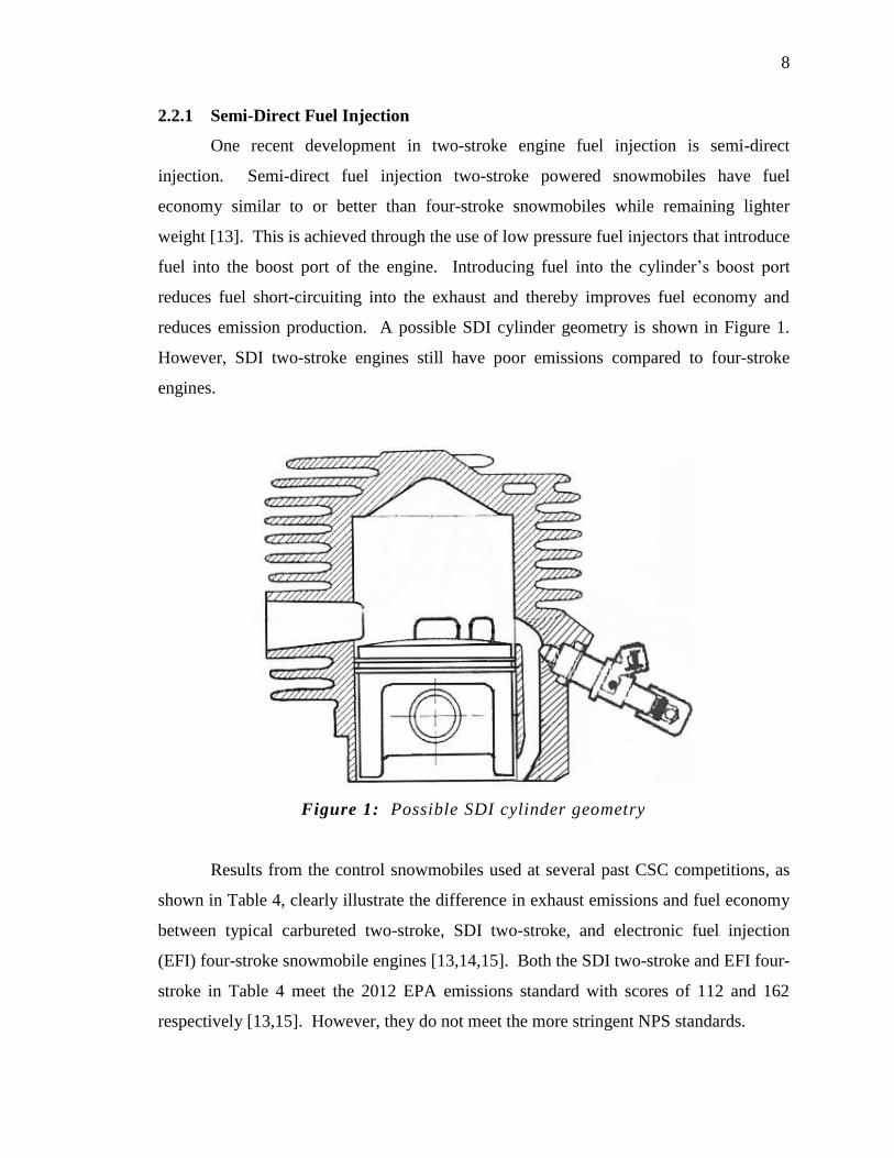
2.2.1 Semi-Direct Fuel Injection

One recent development in two-stroke engine fuel injection is semi-direct

injection. Semi-direct fuel injection two-stroke powered snowmobiles have fuel

economy similar to or better than four-stroke snowmobiles while remaining lighter

weight [13]. This is achieved through the use of low pressure fuel injectors that introduce

fuel into the boost port of the engine. Introducing fuel into the cylinder’s boost port

reduces fuel short-circuiting into the exhaust and thereby improves fuel economy and

reduces emission production. A possible SDI cylinder geometry is shown in Figure 1.

However, SDI two-stroke engines still have poor emissions compared to four-stroke

engines.

Figure 1: Possible SDI cylinder geometry

Results from the control snowmobiles used at several past CSC competitions, as

shown in Table 4, clearly illustrate the difference in exhaust emissions and fuel economy

between typical carbureted two-stroke, SDI two-stroke, and electronic fuel injection

(EFI) four-stroke snowmobile engines [13,14,15]. Both the SDI two-stroke and EFI four-

stroke in Table 4 meet the 2012 EPA emissions standard with scores of 112 and 162

respectively [13,15]. However, they do not meet the more stringent NPS standards.

9

Table 4: Five-Mode Emissions and Fuel Economy of Two and

Four-Stroke CSC Control Snowmobiles

Engine Type CO

[g/kW-hr]

UHC

[g/kW-hr]

NOx

[g/kW-hr]

Fuel Econ.

[MPG]

Two-Stroke Carbureted 319.94 125.50 0.73 8.7

Four-Stroke EFI 99.84 11.48 23.33 15.3

Two-Stroke SDI 215.38 63.53 2.39 19.1

2.2.2 Gasoline Direct Injection

In a GDI two-stroke, fuel is injected directly into the cylinder at an optimal time

for complete mixing and combustion. Air-assisted or high-pressure fuel injectors are

used to ensure the fuel enters the combustion chamber in small droplets so the fuel can

atomize quickly and mix with the freshly scavenged air. It lessens the effects of charge

and exhaust-gas mixing, significantly reduces short-circuiting, and offers precise air/fuel

ratio control. GDI is also known to improve cold start reliability [16]. Additionally, two

different modes of combustion can be used for GDI engines: stratified and homogeneous.

Stratified combustion in a two-stroke GDI is achieved when fuel injection occurs

late in the cycle and ignition is delayed from the start of injection until there is a fuel rich

mixture surrounding the spark plug. The rich condition occurring at the start of ignition

provides a reaction rate high enough to initiate combustion [16]. The flame front occurs

at the interface between the fuel and oxidant, moving out from the spark plug gap burning

the ever-leaner mixture until combustion can no longer be sustained [17]. Stratified

combustion eliminates poor idle quality and poor low load operation [16]. Strauss [7]

suggests using stratified charge combustion during idle and light load operation.

A GDI system can also create a homogeneously charged combustion chamber.

For the GDI engine, homogeneous operation is accomplished when fuel is injected early

in the cycle so there is time for the fuel to completely atomize and mix with the freshly

scavenged air. Homogeneous combustion is used for medium to high loads and is

accomplished two ways. The first is during medium loads. The fuel is injected early and

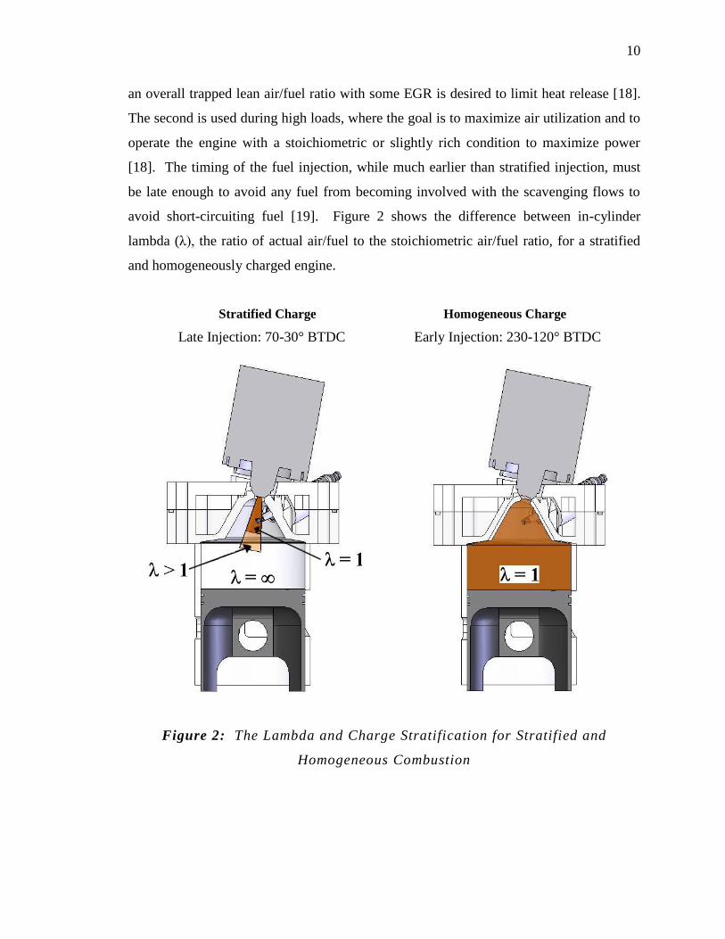
10

an overall trapped lean air/fuel ratio with some EGR is desired to limit heat release [18].

The second is used during high loads, where the goal is to maximize air utilization and to

operate the engine with a stoichiometric or slightly rich condition to maximize power

[18]. The timing of the fuel injection, while much earlier than stratified injection, must

be late enough to avoid any fuel from becoming involved with the scavenging flows to

avoid short-circuiting fuel [19]. Figure 2 shows the difference between in-cylinder

lambda (λ), the ratio of actual air/fuel to the stoichiometric air/fuel ratio, for a stratified

and homogeneously charged engine.

Stratified Charge Homogeneous Charge

Late Injection: 70-30° BTDC Early Injection: 230-120° BTDC

Figure 2: The Lambda and Charge Stratification for Stratified and

Homogeneous Combustion

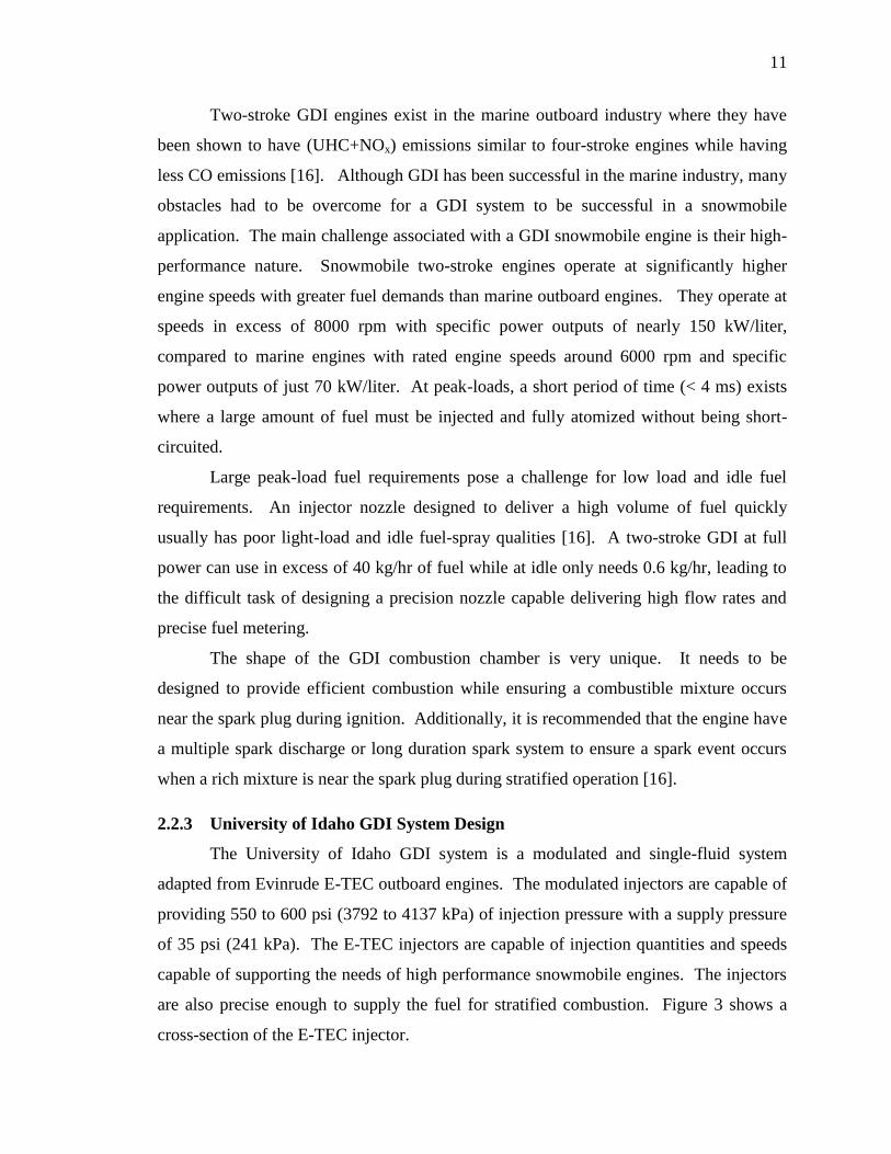
11

Two-stroke GDI engines exist in the marine outboard industry where they have

been shown to have (UHC+NOx) emissions similar to four-stroke engines while having

less CO emissions [16]. Although GDI has been successful in the marine industry, many

obstacles had to be overcome for a GDI system to be successful in a snowmobile

application. The main challenge associated with a GDI snowmobile engine is their high-

performance nature. Snowmobile two-stroke engines operate at significantly higher

engine speeds with greater fuel demands than marine outboard engines. They operate at

speeds in excess of 8000 rpm with specific power outputs of nearly 150 kW/liter,

compared to marine engines with rated engine speeds around 6000 rpm and specific

power outputs of just 70 kW/liter. At peak-loads, a short period of time (< 4 ms) exists

where a large amount of fuel must be injected and fully atomized without being short-

circuited.

Large peak-load fuel requirements pose a challenge for low load and idle fuel

requirements. An injector nozzle designed to deliver a high volume of fuel quickly

usually has poor light-load and idle fuel-spray qualities [16]. A two-stroke GDI at full

power can use in excess of 40 kg/hr of fuel while at idle only needs 0.6 kg/hr, leading to

the difficult task of designing a precision nozzle capable delivering high flow rates and

precise fuel metering.

The shape of the GDI combustion chamber is very unique. It needs to be

designed to provide efficient combustion while ensuring a combustible mixture occurs

near the spark plug during ignition. Additionally, it is recommended that the engine have

a multiple spark discharge or long duration spark system to ensure a spark event occurs

when a rich mixture is near the spark plug during stratified operation [16].

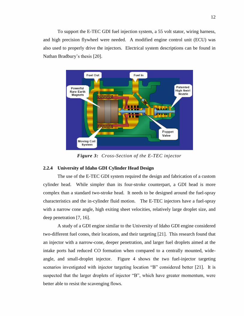
2.2.3 University of Idaho GDI System Design

The University of Idaho GDI system is a modulated and single-fluid system

adapted from Evinrude E-TEC outboard engines. The modulated injectors are capable of

providing 550 to 600 psi (3792 to 4137 kPa) of injection pressure with a supply pressure

of 35 psi (241 kPa). The E-TEC injectors are capable of injection quantities and speeds

capable of supporting the needs of high performance snowmobile engines. The injectors

are also precise enough to supply the fuel for stratified combustion. Figure 3 shows a

cross-section of the E-TEC injector.

12

To support the E-TEC GDI fuel injection system, a 55 volt stator, wiring harness,

and high precision flywheel were needed. A modified engine control unit (ECU) was

also used to properly drive the injectors. Electrical system descriptions can be found in

Nathan Bradbury’s thesis [20].

Figure 3: Cross-Section of the E-TEC injector

2.2.4 University of Idaho GDI Cylinder Head Design

The use of the E-TEC GDI system required the design and fabrication of a custom

cylinder head. While simpler than its four-stroke counterpart, a GDI head is more

complex than a standard two-stroke head. It needs to be designed around the fuel-spray

characteristics and the in-cylinder fluid motion. The E-TEC injectors have a fuel-spray

with a narrow cone angle, high exiting sheet velocities, relatively large droplet size, and

deep penetration [7, 16].

A study of a GDI engine similar to the University of Idaho GDI engine considered

two-different fuel cones, their locations, and their targeting [21]. This research found that

an injector with a narrow-cone, deeper penetration, and larger fuel droplets aimed at the

intake ports had reduced CO formation when compared to a centrally mounted, wide-

angle, and small-droplet injector. Figure 4 shows the two fuel-injector targeting

scenarios investigated with injector targeting location “B” considered better [21]. It is

suspected that the larger droplets of injector “B”, which have greater momentum, were

better able to resist the scavenging flows.

13

Figure 4: Loop-Scavenged GDI Engine Fuel-Spray Targeting Strategies

Another study, based on the E-TEC injectors, offered more insight into injector

targeting, droplet size, and UHC emissions [22]. This study showed that in-cylinder

mixture distribution is largely driven by the momentum exchange between the fuel-spray

and the scavenging flows. The study showed that larger droplets are less affected by

airflows than smaller droplets. A snowmobile two-stroke engine has very aggressive port

geometry that causes intense scavenging flows during high loads. For this reason, an

injector with larger droplets targeted deep into the cylinder can provide good mixture

preparation without excessive UHC emissions during homogeneous combustion.

Strauss [7] shows that wall impingement of the fuel-spray is a major source of

UHC emissions. He also shows that near-nozzle geometry and especially the distance of

the fuel cone from the cylinder wall are critical for optimal fuel-spray development and

mixture preparation. During homogeneous combustion, the geometry of the combustion

chamber, piston, and ports need to work together to aid in complete mixing of the fuel

and air while keeping short-circuited fuel to a minimum. During stratified operation, a

fuel rich condition needs to exist near the spark plug for combustion to occur.

With these factors in mind, the GDI head was modeled using the bolt pattern and

coolant passage patterns from the baseline head. The combustion chamber geometry was

designed to promote stratified operation and even fuel mixing. Near injector nozzle

geometry was improved by using a larger dome radius and chamfer at the injector nozzle

location. In-cylinder flow characteristics were improved by the increasing the dome and

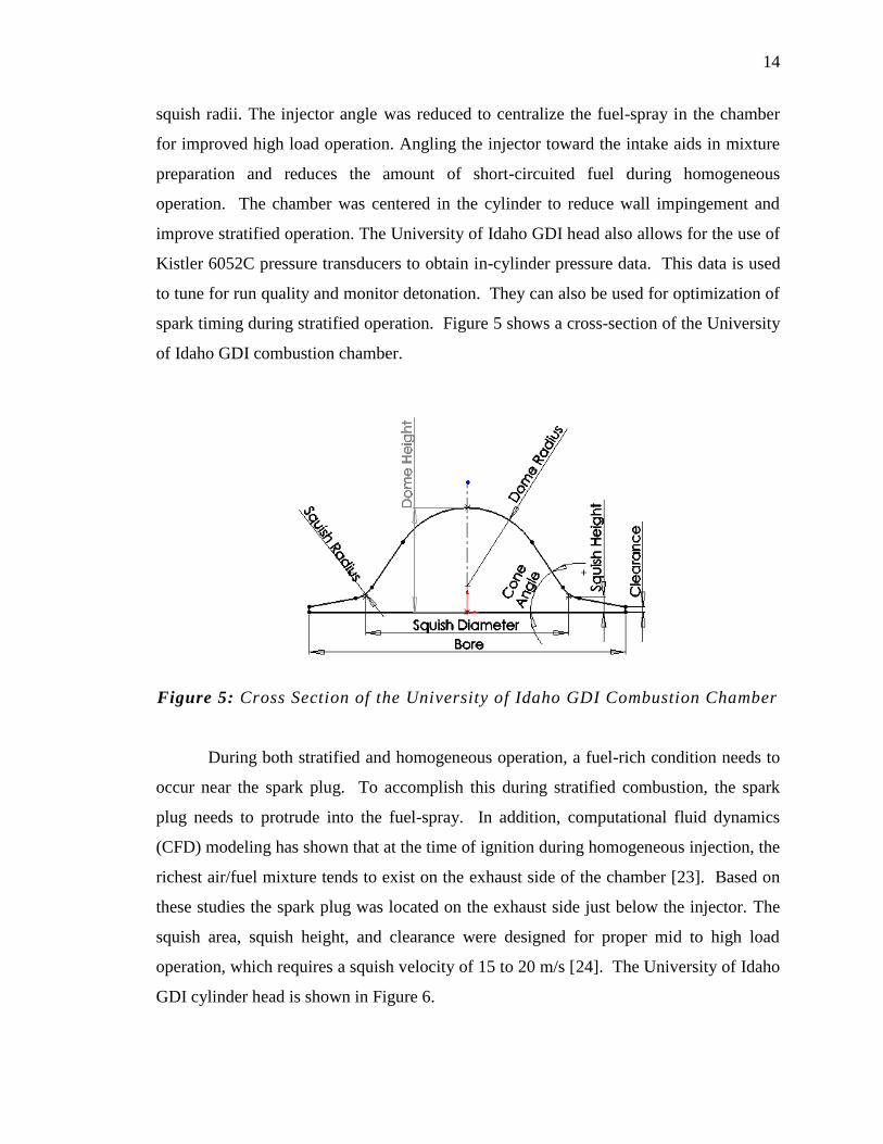
14

squish radii. The injector angle was reduced to centralize the fuel-spray in the chamber

for improved high load operation. Angling the injector toward the intake aids in mixture

preparation and reduces the amount of short-circuited fuel during homogeneous

operation. The chamber was centered in the cylinder to reduce wall impingement and

improve stratified operation. The University of Idaho GDI head also allows for the use of

Kistler 6052C pressure transducers to obtain in-cylinder pressure data. This data is used

to tune for run quality and monitor detonation. They can also be used for optimization of

spark timing during stratified operation. Figure 5 shows a cross-section of the University

of Idaho GDI combustion chamber.

Figure 5: Cross Section of the University of Idaho GDI Combustion Chamber

During both stratified and homogeneous operation, a fuel-rich condition needs to

occur near the spark plug. To accomplish this during stratified combustion, the spark

plug needs to protrude into the fuel-spray. In addition, computational fluid dynamics

(CFD) modeling has shown that at the time of ignition during homogeneous injection, the

richest air/fuel mixture tends to exist on the exhaust side of the chamber [23]. Based on

these studies the spark plug was located on the exhaust side just below the injector. The

squish area, squish height, and clearance were designed for proper mid to high load

operation, which requires a squish velocity of 15 to 20 m/s [24]. The University of Idaho

GDI cylinder head is shown in Figure 6.

15

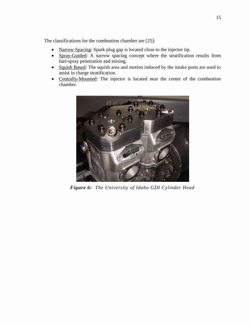
The classifications for the combustion chamber are [25]:

Narrow Spacing: Spark plug gap is located close to the injector tip.

Spray-Guided: A narrow spacing concept where the stratification results from

fuel-spray penetration and mixing.

Squish Based: The squish area and motion induced by the intake ports are used to

assist in charge stratification.

Centrally-Mounted: The injector is located near the center of the combustion

chamber.

Figure 6: The University of Idaho GDI Cylinder Head

16

3.0 BLENDED ETHANOL FUELS

Ethanol has been added to gasoline as an “oxygenate” for decades. Since the

introduction of blended ethanol fuels, their relative performance and environmental

impact has been debated. Ethanol, also known as ethyl alcohol, has very different

physical and combustion characteristics than gasoline. Some properties of both ethanol

and gasoline are outlined in Table 5 [26]. These characteristics cause ethanol fuel’s

physical properties, combustion properties, and hazardous emissions to vary from those

of gasoline. Typically, it is said that blended ethanol fuels introduce more oxygen into

the fuel mixture and therefore the efficiency of combustion is improved. Realistically,

the combustion and emission formation is much more complex [27]. This variation

causes blended ethanol fuels to produce different emissions from gasoline. The

properties of ethanol vary significantly from gasoline and affect energy content, octane,

cold start ability, etc. In this chapter, the environmental impact and properties of blended

ethanol fuels are discussed. These aspects will be compared to that of pure gasoline (E0).

Overall, ethanol has both drawbacks and benefits when compared to gasoline.

Table 5: Properties of Gasoline and Ethanol

Property Gasoline Ethanol

Chemical formula C4-C12 C2H3OH

Molecular weight 100-105 46

Oxygen (mass %) 0-4 34.7

Net lower heating value (MJ/kg) 43.5 27

Latent heat (kJ/L) 223.2 725.4

Stoichiometric air/fuel ratio 14.6 9

Vapor pressure at 23.5 °C (kPa) 60-90 17

MON 82-92 92

RON 91-100 111

3.1 ENVIRONMENTAL IMPACTS OF BLENDED ETHANOL FUELS

Both evaporative and combustion emissions are detrimental to the environment.

When evaporative emissions of raw fuel enter the atmosphere, it causes the formation of

ozone (O3) and possibly photochemical smog [27]. Evaporative emissions come from

anywhere raw fuel is stored such as lines, pumps, tanks, etc. Tailpipe emissions come

from the combustion of fuel in an engine. Depending on the design, type of fuel burned,

17

and emissions control equipment, engines produce different levels of hazardous

emissions. Both evaporative and tailpipe emissions will be discussed with respect to

blended ethanol fuels.

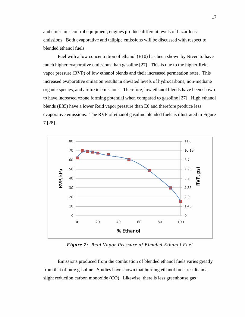
Fuel with a low concentration of ethanol (E10) has been shown by Niven to have

much higher evaporative emissions than gasoline [27]. This is due to the higher Reid

vapor pressure (RVP) of low ethanol blends and their increased permeation rates. This

increased evaporative emission results in elevated levels of hydrocarbons, non-methane

organic species, and air toxic emissions. Therefore, low ethanol blends have been shown

to have increased ozone forming potential when compared to gasoline [27]. High ethanol

blends (E85) have a lower Reid vapor pressure than E0 and therefore produce less

evaporative emissions. The RVP of ethanol gasoline blended fuels is illustrated in Figure

7 [28].

Figure 7: Reid Vapor Pressure of Blended Ethanol Fuel

Emissions produced from the combustion of blended ethanol fuels varies greatly

from that of pure gasoline. Studies have shown that burning ethanol fuels results in a

slight reduction carbon monoxide (CO). Likewise, there is less greenhouse gas

18

production due to CO [27]. There is also a reduction in unburned hydrocarbon (UHC)

emissions from burning ethanol fuels [26]. While there is a reduction in CO and UHC

production, it has been shown that burning blended ethanol fuels increases the production

of oxides of nitrogen (NOx) and other harmful emissions such as acetaldehydes,

formaldehydes, and ethanol. This increase in NOx emissions results in increased

photochemical smog and ground-level ozone [27].

Blended ethanol fuels produce greatly increased levels of toxic emissions such as

acetaldehydes and formaldehydes. Compared to E0, acetaldehyde production was

increased one to seven times with E10 and up to 27 times with E85. Acetaldehyde is

known as very hazardous and a probable carcinogen. It is also a precursor to

peroxylacetate nitrate (PAN) which is a respiratory irritant and known plant toxin [27].

Tests of a two-stroke chainsaw engine running on a low ethanol blend (E15) resulted in a

substantial increase in formaldehyde emissions [27]. Formaldehyde production is also

significantly increased with E85 fuel [27]. In both E10 and E85 the emission of ethanol

was also greatly increased over E0 [27]. In typical automotive applications, a catalytic

converter is used to break down emissions produced from combustion. Catalytic

converters are typically designed to reduce CO, UHC, and NOx emissions. The added

emissions of blended ethanol fuels, such as formaldehyde, ethanol, and acetaldehyde,

resist breakdown in catalytic converters [27].

Emission production can also be studied over the total lifecycle of the fuel.

Carbon dioxide formation and particulate emissions of blended ethanol fuels are

significantly higher than E0 when totaled over the entire fuel lifecycle. This increase is

mostly due to agricultural activities such as burning fields [27].

3.2 PROPERTIES OF BLENDED ETHANOL FUELS

The properties of blended ethanol vary from that of gasoline. These variations

effect how an engine must be designed to properly burn blended ethanol fuels. The main

differences that will be discussed in this section are energy content, flame development,

octane rating, cold start properties, oxygen content, shelf life, and corrosive properties.

The energy content of ethanol fuel will be the first property discussed. Ethanol

and gasoline have lower heating values (LHV) of 27 MJ/kg and 43.5 MJ/kg respectively.

When a mixture of 85% ethanol/15% gasoline is blended, a LHV of approximately 29.5

19

MJ/kg is created. From these LHVs it can be seen that E85 has approximately 68% of

the energy of gasoline. If an engine is converted from gasoline to E85 fuel it will either

produce ~30% less power or it will burn ~30% more fuel to produce an equal amount of

power. Typically, the amount of fuel is increased to achieve the proper air-fuel ratio and

produce an equivalent power output.

In addition to quantity modifications, spark timing may also have to be modified

for blended ethanol fuels. High ethanol content fuels have shown to take longer to

develop a stable flame, but once developed, the combustion duration was similar to that

of gasoline [29]. Due to this, spark timing may need to be advanced for peak cylinder

pressure to occur at the correct time for efficient conversion to mechanical work.

The octane rating of ethanol fuel will be the next item discussed. There are two

different octane ratings: Research Octane Number (RON) and Motor Octane Number

(MON). In the United States fuel octane is usually reported as an Anti-Knock Index

(AKI) or the average of the RON and MON. Unleaded pump gasoline in the United

States usually has an AKI of 84 to 91, while E85 has an AKI of 101 to 105 [30]. This

higher octane rating is related to the higher activation energy of ethanol fuels. Ethanol

fuels require more energy to start a chemical reaction, and are therefore less prone to

auto-ignition and detonation. The compression ratio can be safely increased when

combusting high ethanol content fuels. It has been shown by Blair that in a two-stroke

engine increasing compression ratio will increase power output and decrease fuel

consumption because of increased combustion efficiency [24]. Increasing the

compression ratio will increase efficiency and partially mitigate the lower energy content

of high ethanol fuel blends.

In snowmobile applications, a main concern of using blended ethanol fuel is its

poor cold start characteristics. At 725.4 kg/L, ethanol has a much higher latent heat than

gasoline, which is 223.2 kg/L [26]. Latent heat is the amount of energy that is required or

produced during a phase change, in this case from a liquid to a gas. Fuels with a higher

latent heat pull more energy out of the incoming air charge during vaporization. This

cools the incoming air charge and leads to higher intake charge density and lower

combustion temperatures. This effect is beneficial in high performance engines at steady

state, but is detrimental during cold start. When the engine and incoming charge are at

20

low temperatures there is often not enough energy present to vaporize and combust

blended ethanol fuels. This causes poor cold start characteristics.

Another major concern when using blended ethanol fuels in any application is that

it is much more corrosive than pure gasoline. Much of the fuel system in a typical

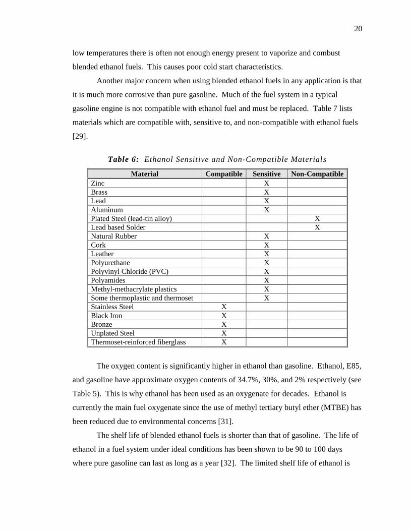
gasoline engine is not compatible with ethanol fuel and must be replaced. Table 7 lists

materials which are compatible with, sensitive to, and non-compatible with ethanol fuels

[29].

Table 6: Ethanol Sensitive and Non-Compatible Materials

Material Compatible Sensitive Non-Compatible

Zinc X

Brass X

Lead X

Aluminum X

Plated Steel (lead-tin alloy) X

Lead based Solder X

Natural Rubber X

Cork X

Leather X

Polyurethane X

Polyvinyl Chloride (PVC) X

Polyamides X

Methyl-methacrylate plastics X

Some thermoplastic and thermoset X

Stainless Steel X

Black Iron X

Bronze X

Unplated Steel X

Thermoset-reinforced fiberglass X

The oxygen content is significantly higher in ethanol than gasoline. Ethanol, E85,

and gasoline have approximate oxygen contents of 34.7%, 30%, and 2% respectively (see

Table 5). This is why ethanol has been used as an oxygenate for decades. Ethanol is

currently the main fuel oxygenate since the use of methyl tertiary butyl ether (MTBE) has

been reduced due to environmental concerns [31].

The shelf life of blended ethanol fuels is shorter than that of gasoline. The life of

ethanol in a fuel system under ideal conditions has been shown to be 90 to 100 days

where pure gasoline can last as long as a year [32]. The limited shelf life of ethanol is

21

due to its affinity for water. When a vehicle is subjected to conditions of rain and snow

the life of ethanol is significantly reduced.

3.3 ENGINE SYSTEM DESIGN FOR BLENDED ETHANOL FUELS

Internal combustion engines that are designed to burn pure gasoline (E0) are not

properly equipped to run high blends of ethanol. Fuels with low percentages of ethanol

(E10) can be burned in standard production gasoline engines without detrimental effects.

To efficiently and effectively burn fuels with large percentages of ethanol, typical

production gasoline engines must be modified. These modifications include material

changes to prevent corrosion and engine modifications to properly combust blended

ethanol fuels. In flex-fuel systems the addition of an ethanol content sensor is also

necessary.

As discussed in the previous section, fuels with large percentages of ethanol, such

as E85, are very corrosive to fuel systems, so many modifications are required. Stainless

steel must be used to replace most fuel fittings and plain carbon steel components [33].

The fuel lines must be changed to those compatible with alcohol fuels, because traditional

rubber lines are insufficient. Fuel lines that are rated SAE J30R9 are approved for

ethanol inside of the line, while SAE J30R10 fuel lines are rated for ethanol contact on

the inside and outside of the line [34].

The fuel pump must also be changed when converting to the use of high ethanol

blends since high ethanol fuel blends corrode and destroy traditional pumps. Ethanol fuel

pumps often use precious metals such as silver to resist corrosion. In many applications

the fuel pump size must be increased to support the higher volume of fuel required by the

engine.

In addition to fuel system modifications, gasoline engines should be modified to

more efficiently burn fuels with high ethanol content. As discussed previously, ethanol

has a lower energy value than that of pure gasoline, so larger volumes of ethanol must be

burned to produce the same amount of power as pure gasoline. This often requires the

use of larger injectors with higher flow rates. Even though larger amounts must be

injected, the spray properties of ethanol fuels have been shown to be very similar to that

of gasoline. Using swirl-type nozzles, the penetration and cone angle are very similar

[35]. In direct injected engines, spray characteristics have a large impact on fuel

22

efficiency, power output, and hazardous emission formation. By having similar spray

properties, fuel injector nozzles and combustion chamber shapes designed to produce

favorable spray characteristics in gasoline engines will also work for blended ethanol

injection.

Blended ethanol fuels require larger volumes to be injected than does gasoline.

This translates to a reduction in fuel efficiency per volume. To partially counteract this

reduction in efficiency, compression ratios can be increased, since ethanol has a higher

knock resistance [38]. Overall engine efficiency increases with increased compression

ratios because of improved combustion efficiency. High compression ratios can be used

with blended ethanol fuels that would cause pure gasoline to detonate and cause severe

engine damage [26, 36].

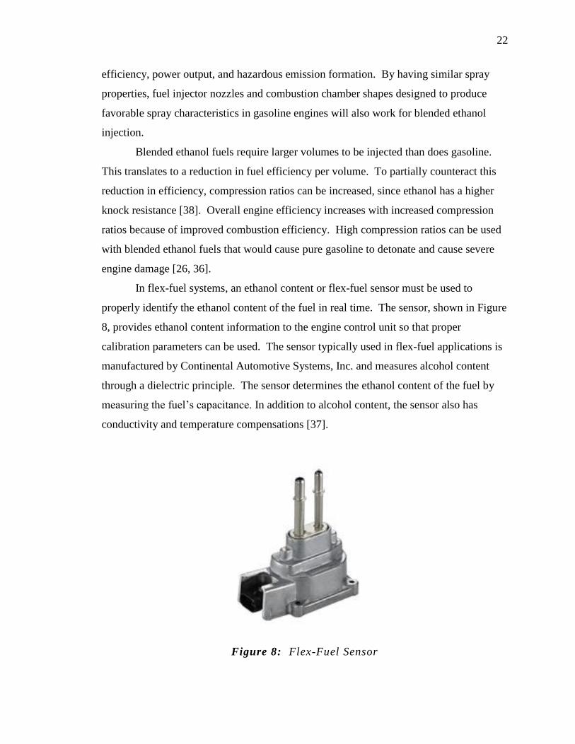
In flex-fuel systems, an ethanol content or flex-fuel sensor must be used to

properly identify the ethanol content of the fuel in real time. The sensor, shown in Figure

8, provides ethanol content information to the engine control unit so that proper

calibration parameters can be used. The sensor typically used in flex-fuel applications is

manufactured by Continental Automotive Systems, Inc. and measures alcohol content

through a dielectric principle. The sensor determines the ethanol content of the fuel by

measuring the fuel’s capacitance. In addition to alcohol content, the sensor also has

conductivity and temperature compensations [37].

Figure 8: Flex-Fuel Sensor

23

4.0 UNIVERSTIY OF IDAHO ENGINE SYSTEM DESIGN

The University of Idaho engine system design is based on the properties and

requirements of blended ethanol fuel. Ideally the engine hardware would be modified to

properly combust blended ethanol. The trapped compression ratio should be increased

for high ethanol blends. The University of Idaho engine system needed to be designed

for the use of flex-fuel and therefore the trapped compression ratio was not increased so

that the engine package could safely run on both E0 and E85. To take advantage of the

high knock resistance of high ethanol blends, a flex-fuel system would need to have

variable compression. Due to the complexity, cost, and development time required for a

variable compression engine it was determined that it was not feasible. The University of

Idaho GDI cylinder head was also not modified for blended ethanol fuel. This was due to

the similarity in fuel-spray properties of gasoline and ethanol.

The main engine system changes for blended ethanol involved the fuel injection

system, fuel system, and calibration strategies. The proper fuel injection system was

chosen to best suit the fuel consumed. The fuel system was modified to resist the

corrosive properties of ethanol and properly deliver the fuel to the engine. The

calibration strategies were based on the flame development, energy content, and cold start

properties of blended ethanol fuel. The fuel injection selection, fuel system modifications

and calibration strategies are discussed in this chapter.

4.1 FUEL INJECTION SELECTION

The ethanol blends examined in this work are winter blend E85 and flex-fuel.

The conversion to winter blend E85 for the 2008 CSC competition required engine

modifications and calibration changes. Gasoline direct injection easily supported this

change because no engine controller software or hardware modification was necessary.

To support flex-fuel, a continuous ethanol content feedback loop is required.

The 2009 CSC rules mandated the use of flex-fuel, which requires continuous

ethanol content feedback to the engine controller. This feedback alters the engine’s

calibration strategy to efficiently combust the blend of ethanol fuel in the system. While

gasoline direct injection is very clean and efficient, it also requires a complex electronic

control system for proper operation. UICSC’s 2008 GDI control unit would not

accommodate in-service fuel changes. Due to time and resource constraints, it was

24

determined that a GDI system with ethanol content feedback was not feasible for flex-

fuel operation. Instead, the UICSC team decided to use an SDI platform, which uses a

standard fuel injection controller. An SDI two-stroke maintains a high power-to-weight

ratio and offers improved emissions and fuel economy over carbureted and throttle body

injected two-stroke engines.

4.2 FUEL SYSTEM

The fuel system was modified to resist the corrosive properties of ethanol fuels.

The fuel lines and fuel pump were changed and an in-line fuel filter was added. The fuel

pickup line inside of the fuel tank was changed to a SAE J30R10 rated fuel line so that

the ethanol did not corrode the inside or outside of the fuel line. The remaining fuel lines

were replaced with a SAE J30R9 fuel line that is rated for ethanol on the inside of the

fuel line [34]. The fuel pump selected for the ethanol fuel system was a Bosch in-line

flex-fuel pump. An in-line fuel filter was added to the system due to the particulate

matter that was found in the blended ethanol fuel. Due to the corrosive properties of

ethanol, the fuel breaks down many materials that it contacts during transport and

storage. Many of these materials then flake and become particulate in the fuel. If

particulate is not filtered, it can lead to clogged fuel injectors.

4.3 FLEX-FUEL SYSTEM

The University of Idaho flex-fuel system uses a Continental Automotive Systems,

Inc. flex-fuel sensor as shown in Figure 8. The flex-fuel sensor uses dielectrics to

determine the ethanol content of the fuel and then outputs the ethanol content as a

frequency. The frequency output varies from 50 to 150 Hz corresponding to the ethanol

content of the fuel. This curve is shown in Figure 9. To input the ethanol content

information into the engine controller, the frequency output had to be conditioned into a 0

to 5 volt signal. This was accomplished through the use of an analog frequency to

voltage converter chip and a custom designed circuit that was designed and built by

members of the 2009 University of Idaho CSC team. The frequency to voltage circuit

also displayed the ethanol content on a LED display on the dash of the snowmobile. The

LED ethanol content display is shown in Figure 10.

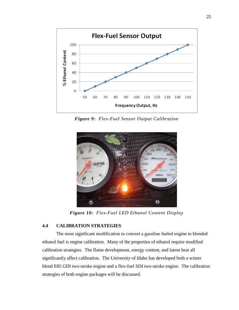
25

Figure 9: Flex-Fuel Sensor Output Calibration

Figure 10: Flex-Fuel LED Ethanol Content Display

4.4 CALIBRATION STRATEGIES

The most significant modification to convert a gasoline fueled engine to blended

ethanol fuel is engine calibration. Many of the properties of ethanol require modified

calibration strategies. The flame development, energy content, and latent heat all

significantly affect calibration. The University of Idaho has developed both a winter

blend E85 GDI two-stroke engine and a flex-fuel SDI two-stroke engine. The calibration

strategies of both engine packages will be discussed.

26

4.4.1 Winter Blend E85 GDI Two-Stroke Engine

The University of Idaho GDI two-stroke engine was calibrated for a low blend

ethanol fuel (E10) prior to this work. This engine calibration produced sufficient power

output, good fuel economy, and low emissions. This meant that all calibration work

could focus on converting to winter blend E85. As discussed before, the GDI system is

capable of two different modes of combustion: homogeneous and stratified. The GDI

two-stroke engine runs stratified at idle and below clutch engagement. Homogeneous

combustion is utilized at all the other operating points. The main calibration parameters

for a GDI two-stroke engine are fuel quantity, fuel timing, and ignition timing. All of

these parameters were calibrated for blended ethanol fuels during both stratified and

homogeneous modes of combustion. The calibration parameters were optimized based

on engine efficiency, fuel economy, and performance. Emission production was not

studied due to the lack of sufficient equipment.

The first parameter adjusted was the fuel quantity. Fuel quantity was increased

to compensate for the low energy content of blended ethanol fuels. The lower heating

value (LHV) of ethanol is 27 MJ/kg, while the LHV of gasoline is 43.5 MJ/kg. A

mixture of 75% ethanol/25% gasoline creates a LHV of approximately 31.12 MJ/kg.

Therefore, winter blend E85 has approximately 72% of the energy of gasoline and the

quantity of fuel had to be adjusted appropriately. The entire fuel quantity map was

increased by approximately 30% and then the individual calibration points were fine

tuned for the high ethanol blend. Fuel quantity was calibrated based on exhaust lambda

measurements. Lambda measurement with respect to blended ethanol fuels will be

discussed in section 5.1.2.

In a GDI two-stroke engine, injection timing is very important for fuel economy,

performance, power delivery, and emission production. When the injected fuel quantity

is increased, the duration of injection is also increased and therefore the injection timing

is affected. In a GDI system, injection timing is a very precise balance between injecting

soon enough to obtain proper mixing while trying to inject late enough to minimize short-

circuiting. The later fuel is injected, the less quantity is required and therefore emission

production and fuel consumption will be reduced. The proper fuel injection timing was

27

determined through the use of lambda measurement and brake specific fuel consumption

(BSFC) sweeps, which will be discussed in section 5.1.1.

Blended ethanol fuels take longer to develop a stable flame then gasoline, so

ignition timing was examined during calibration [28]. It was found that high blends of

ethanol allowed the ignition timing to be advanced significantly before the onset of

detonation. This is partially due to the flame development time and the knock resistance

of the blended ethanol fuel. It was found that advancing ignition timing significantly

increased BSFC and performance at part load cruise and high loads/speeds.

The increased latent heat of ethanol fuels was examined with respect to stratified

operation in the GDI two-stroke engine. It was found that the increased latent heat of

ethanol did not substantially reduce the cold start ability of the GDI engine. This is due

to the already improved cold start ability inherent in stratified combustion [16].

4.4.2 Flex-Fuel SDI Two-Stroke Engine

The Rotax SDI two-stroke engine platform was selected for conversion to blended

ethanol flex-fuel. This platform was selected because it uses automotive style fuel

injectors that can be controlled with a standard engine control unit. To incorporate the

flex-fuel feedback system described before, a custom ECU was used. This ECU allowed

for injection quantity and ignition timing ethanol content compensation maps. Before

any flex-fuel calibration could be performed, the base engine control maps had to be

created. The main calibration parameters of an SDI two-stroke engine are injection

quantity, injection timing, and ignition timing. The calibration strategies associated with

creating the base maps and the flex-fuel correction will be discussed in this section.

The calibration parameters were measured from the original equipment

manufacturer (OEM) SDI engine to create the base maps. The engine was run through all

of its operating points on a dynamometer while a oscilloscope and timing light were used

to measure ignition timing, injection quantity, and injection timing. The spark timing

was measured with the timing light. The injection quantity is controlled by the pulse

width of the driving signal. This pulse width was measured with the oscilloscope. The

injection signal and ignition signal timing were also analyzed with the oscilloscope.

Knowing the ignition timing allowed the injection timing to be calculated from the

oscilloscope data. With these base values, the flex-fuel SDI engine was then fine tuned

28

for performance, BSFC, and overall smooth power delivery on a low blend of ethanol

fuel (E10).

Once the base E10 maps were calibrated, a flex-fuel compensation map was

created. The flex-fuel compensation map multiplies the E10 injection quantity based on

the ethanol content of the fuel. Initial compensation values were calculated based on the

energy content of the ethanol blend. The flex-fuel compensation map was then calibrated

for performance and BSFC using various blends of ethanol and gasoline.

The ignition timing and injection timing were both analyzed with respect to

different blends of ethanol and gasoline. In an SDI two-stroke engine fuel is injected into

the boost ports. When large quantities are desired, injection starts when the piston is near

top dead center (TDC) and fuel is injected into the crankcase. Due to the nature of the

SDI system, injection timing is not as critical to performance and BSFC as it is to the

GDI system. Injection timing has a large impact on emission production, but due to

facility constraints, emissions were not analyzed. Ignition timing was analyzed with the

SDI, but there was not a significant improvement associated with advancing the spark

timing. A significant change was not seen because of the aggressive base E10 ignition

calibration.

The increased latent heat of ethanol required specific cold start calibration of the

SDI two-stroke engine. To achieve reliable cold start characteristics, the base engine

injection quantity, injection timing, and ignition timing calibration parameters were

adjusted through numerous tuning sessions.

29

5.0 TESTING

The winter blend E85 and the flex-fuel SDI engine packages were rigorously

tested to verify performance, fuel economy, and smooth power delivery. The engines

were calibrated on dynamometer systems to create engine control maps that focused on

power output and brake specific fuel consumption (BSFC). The engine packages were

then dynamically calibrated in-service. Finally, fuel economy, cold start, and power

delivery were verified in-chassis on snowmobile trails.

5.1 METHODOLOGY

During calibration many different tools and measurements were used. The main

tools used were brake specific fuel consumption (BSFC), lambda, and fuel economy.

These tools and measurements are discussed with respect to blended ethanol fuels in this

section.

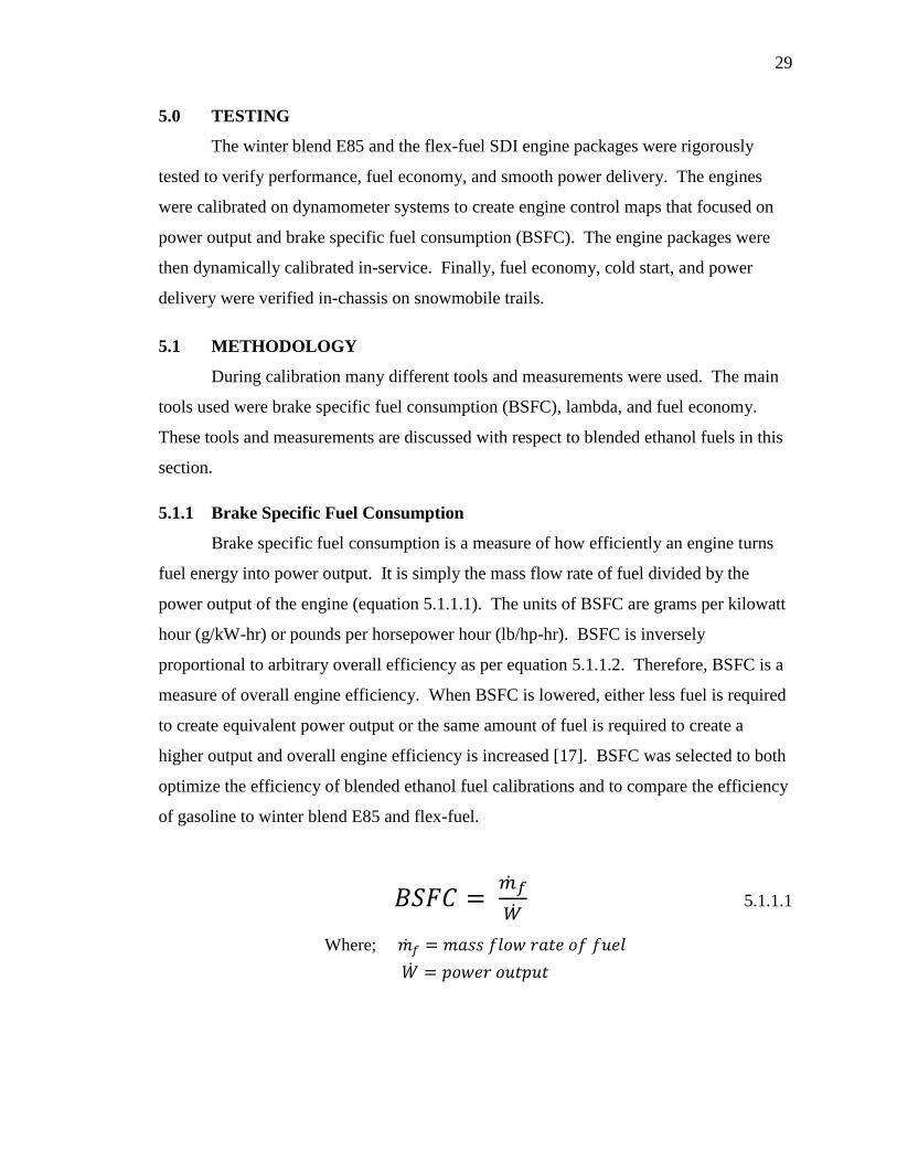
5.1.1 Brake Specific Fuel Consumption

Brake specific fuel consumption is a measure of how efficiently an engine turns

fuel energy into power output. It is simply the mass flow rate of fuel divided by the

power output of the engine (equation 5.1.1.1). The units of BSFC are grams per kilowatt

hour (g/kW-hr) or pounds per horsepower hour (lb/hp-hr). BSFC is inversely

proportional to arbitrary overall efficiency as per equation 5.1.1.2. Therefore, BSFC is a

measure of overall engine efficiency. When BSFC is lowered, either less fuel is required

to create equivalent power output or the same amount of fuel is required to create a

higher output and overall engine efficiency is increased [17]. BSFC was selected to both

optimize the efficiency of blended ethanol fuel calibrations and to compare the efficiency

of gasoline to winter blend E85 and flex-fuel.

5.1.1.1

Where;

30

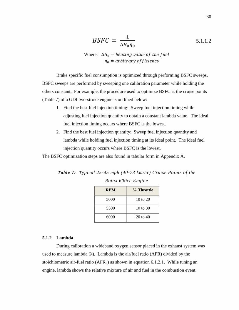
5.1.1.2

Where;

Brake specific fuel consumption is optimized through performing BSFC sweeps.

BSFC sweeps are performed by sweeping one calibration parameter while holding the

others constant. For example, the procedure used to optimize BSFC at the cruise points

(Table 7) of a GDI two-stroke engine is outlined below:

1. Find the best fuel injection timing: Sweep fuel injection timing while

adjusting fuel injection quantity to obtain a constant lambda value. The ideal

fuel injection timing occurs where BSFC is the lowest.

2. Find the best fuel injection quantity: Sweep fuel injection quantity and

lambda while holding fuel injection timing at its ideal point. The ideal fuel

injection quantity occurs where BSFC is the lowest.

The BSFC optimization steps are also found in tabular form in Appendix A.

Table 7: Typical 25-45 mph (40-73 km/hr) Cruise Points of the

Rotax 600cc Engine

RPM % Throttle

5000 10 to 20

5500 10 to 30

6000 20 to 40

5.1.2 Lambda

During calibration a wideband oxygen sensor placed in the exhaust system was

used to measure lambda (λ). Lambda is the air/fuel ratio (AFR) divided by the

stoichiometric air-fuel ratio (AFRS) as shown in equation 6.1.2.1. While tuning an

engine, lambda shows the relative mixture of air and fuel in the combustion event.

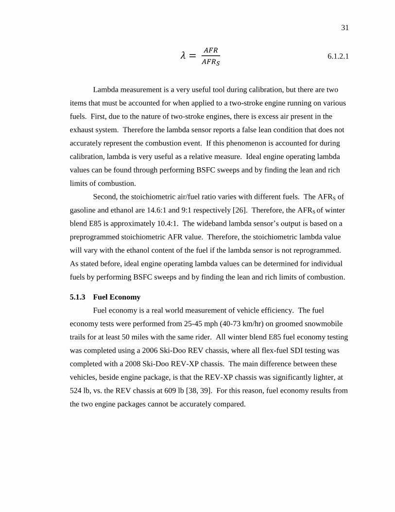
31

6.1.2.1

Lambda measurement is a very useful tool during calibration, but there are two

items that must be accounted for when applied to a two-stroke engine running on various

fuels. First, due to the nature of two-stroke engines, there is excess air present in the

exhaust system. Therefore the lambda sensor reports a false lean condition that does not

accurately represent the combustion event. If this phenomenon is accounted for during

calibration, lambda is very useful as a relative measure. Ideal engine operating lambda

values can be found through performing BSFC sweeps and by finding the lean and rich

limits of combustion.

Second, the stoichiometric air/fuel ratio varies with different fuels. The AFRS of

gasoline and ethanol are 14.6:1 and 9:1 respectively [26]. Therefore, the AFRS of winter

blend E85 is approximately 10.4:1. The wideband lambda sensor’s output is based on a

preprogrammed stoichiometric AFR value. Therefore, the stoichiometric lambda value

will vary with the ethanol content of the fuel if the lambda sensor is not reprogrammed.

As stated before, ideal engine operating lambda values can be determined for individual

fuels by performing BSFC sweeps and by finding the lean and rich limits of combustion.

5.1.3 Fuel Economy

Fuel economy is a real world measurement of vehicle efficiency. The fuel

economy tests were performed from 25-45 mph (40-73 km/hr) on groomed snowmobile

trails for at least 50 miles with the same rider. All winter blend E85 fuel economy testing

was completed using a 2006 Ski-Doo REV chassis, where all flex-fuel SDI testing was

completed with a 2008 Ski-Doo REV-XP chassis. The main difference between these

vehicles, beside engine package, is that the REV-XP chassis was significantly lighter, at

524 lb, vs. the REV chassis at 609 lb [38, 39]. For this reason, fuel economy results from

the two engine packages cannot be accurately compared.

32

5.2 TESTING EQUIPMENT

5.2.1 Water-Brake Dynamometer

A DYNOmite™ toroid flow nine-inch water brake dynamometer, manufactured

by Land and Sea, was used for all GDI calibration work. The dynamometer was used to

apply load and hold the engine at various operating points while measuring torque and

engine speed. The dynamometer system consists of a dynamometer head, load valve,

servo driven throttle control, water pump, water tower, and data acquisition/control

software. The dynamometer head consists of an inner rotor, housing, and torque arm (see

Figure 11). The inner rotor of the dynamometer head attaches directly to the crankshaft

of the engine and the outer housing is fixed through the torque arm. A temperature

compensated full-bridge strain gauge is attached to the torque arm and measures torque to

an accuracy of 0.5% of the full load range. The torque and power ratings of the nine-inch

dynamometer head are shown in Figure 12 [40].

Figure 11: Land and Sea DYNOmite™ Dynamometer Head

The dynamometer head is supplied pressurized water near the center of the

housing. As the engine rotates, the water is accelerated by the rotor to the periphery of

the housing. The water causes viscous friction between the rotor and the housing, which

causes a torque about the crankshaft. This torque is then measured with the strain gauge.

The load on the engine is varied by changing the pressure to the dynamometer head. This

33

pressure is varied by the load valve which can be controlled either manually or through

the dynamometer control software.

The data acquisition/control software has the capability to log various parameters

such as pressures, temperatures, engine speed, torque, power, fuel flow, and many others.

The software also controls the load valve and the servo driven throttle control. For

calibration purposes, the position of the throttle and the engine rpm were specified to the

software. The dynamometer then holds the engine at that speed and load. Due to the

inherent slow response time of the water brake system, the software could not effectively

hold the two-stroke engine at one rpm. Two-stroke engines have low inertia and steep

power curves, which causes the dynamometer to go into a cyclic oscillation. The engine

rpm oscillations were typically 100 rpm but could be as large as 1000 rpm. This proved

to make engine calibration using the water-brake dynamometer nearly impossible. For

this reason, the University of Idaho upgraded to an eddy current dynamometer system.

Figure 12: Torque and Power Ratings of the Dynamometer Head

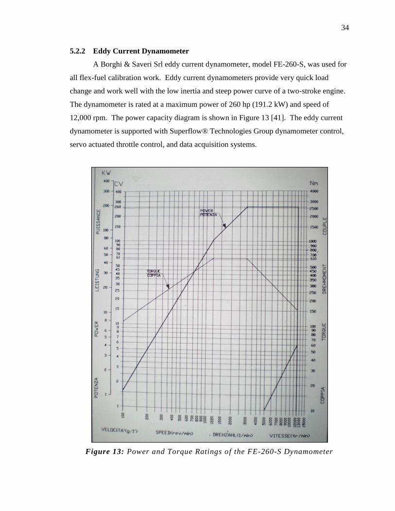
34

5.2.2 Eddy Current Dynamometer

A Borghi & Saveri Srl eddy current dynamometer, model FE-260-S, was used for

all flex-fuel calibration work. Eddy current dynamometers provide very quick load

change and work well with the low inertia and steep power curve of a two-stroke engine.

The dynamometer is rated at a maximum power of 260 hp (191.2 kW) and speed of

12,000 rpm. The power capacity diagram is shown in Figure 13 [41]. The eddy current

dynamometer is supported with Superflow® Technologies Group dynamometer control,

servo actuated throttle control, and data acquisition systems.

Figure 13: Power and Torque Ratings of the FE-260-S Dynamometer

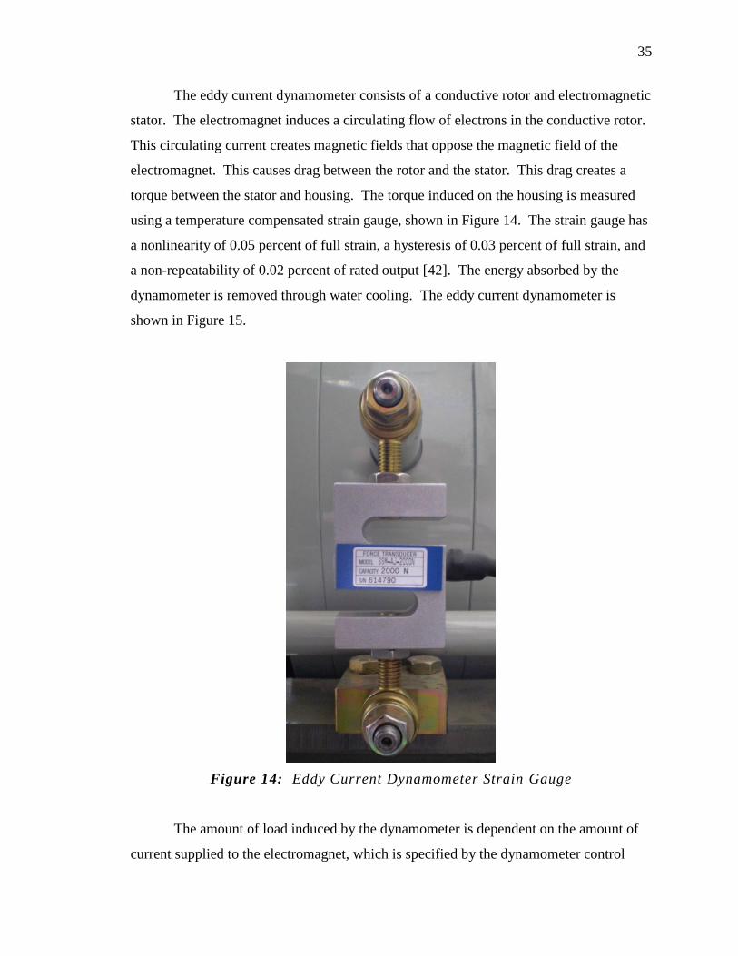
35

The eddy current dynamometer consists of a conductive rotor and electromagnetic

stator. The electromagnet induces a circulating flow of electrons in the conductive rotor.

This circulating current creates magnetic fields that oppose the magnetic field of the

electromagnet. This causes drag between the rotor and the stator. This drag creates a

torque between the stator and housing. The torque induced on the housing is measured

using a temperature compensated strain gauge, shown in Figure 14. The strain gauge has

a nonlinearity of 0.05 percent of full strain, a hysteresis of 0.03 percent of full strain, and

a non-repeatability of 0.02 percent of rated output [42]. The energy absorbed by the

dynamometer is removed through water cooling. The eddy current dynamometer is

shown in Figure 15.

Figure 14: Eddy Current Dynamometer Strain Gauge

The amount of load induced by the dynamometer is dependent on the amount of

current supplied to the electromagnet, which is specified by the dynamometer control

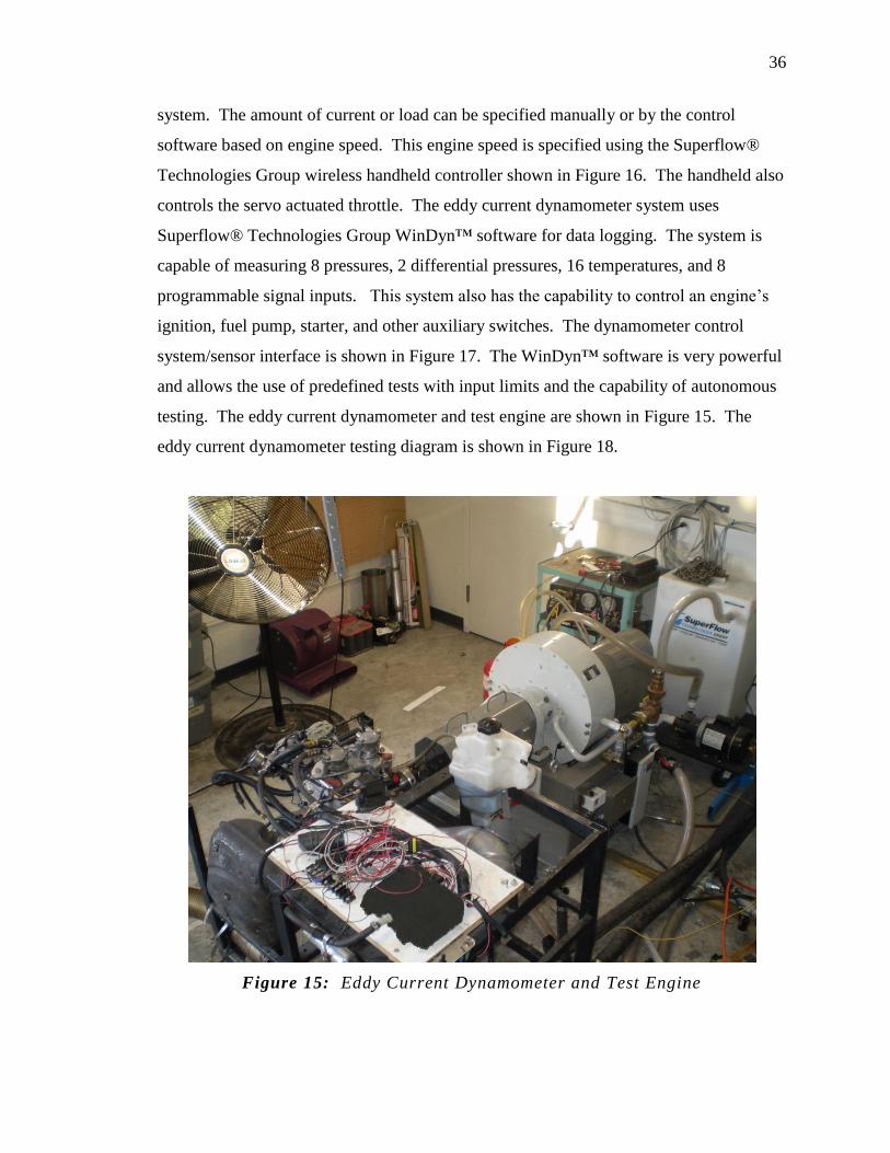
36

system. The amount of current or load can be specified manually or by the control

software based on engine speed. This engine speed is specified using the Superflow®

Technologies Group wireless handheld controller shown in Figure 16. The handheld also

controls the servo actuated throttle. The eddy current dynamometer system uses

Superflow® Technologies Group WinDyn™ software for data logging. The system is

capable of measuring 8 pressures, 2 differential pressures, 16 temperatures, and 8

programmable signal inputs. This system also has the capability to control an engine’s

ignition, fuel pump, starter, and other auxiliary switches. The dynamometer control

system/sensor interface is shown in Figure 17. The WinDyn™ software is very powerful

and allows the use of predefined tests with input limits and the capability of autonomous

testing. The eddy current dynamometer and test engine are shown in Figure 15. The

eddy current dynamometer testing diagram is shown in Figure 18.

Figure 15: Eddy Current Dynamometer and Test Engine

37

Figure 16: Dynamometer Wireless Handheld Controller

Figure 17: Dynamometer Control System/Sensor Interface

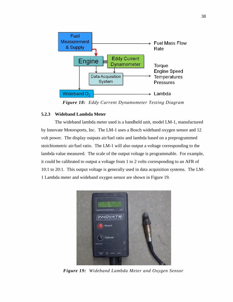
38

Figure 18: Eddy Current Dynamometer Testing Diagram

5.2.3 Wideband Lambda Meter

The wideband lambda meter used is a handheld unit, model LM-1, manufactured

by Innovate Motorsports, Inc. The LM-1 uses a Bosch wideband oxygen sensor and 12

volt power. The display outputs air/fuel ratio and lambda based on a preprogrammed

stoichiometric air/fuel ratio. The LM-1 will also output a voltage corresponding to the

lambda value measured. The scale of the output voltage is programmable. For example,

it could be calibrated to output a voltage from 1 to 2 volts corresponding to an AFR of

10:1 to 20:1. This output voltage is generally used in data acquisition systems. The LM-

1 Lambda meter and wideband oxygen sensor are shown in Figure 19.

Figure 19: Wideband Lambda Meter and Oxygen Sensor

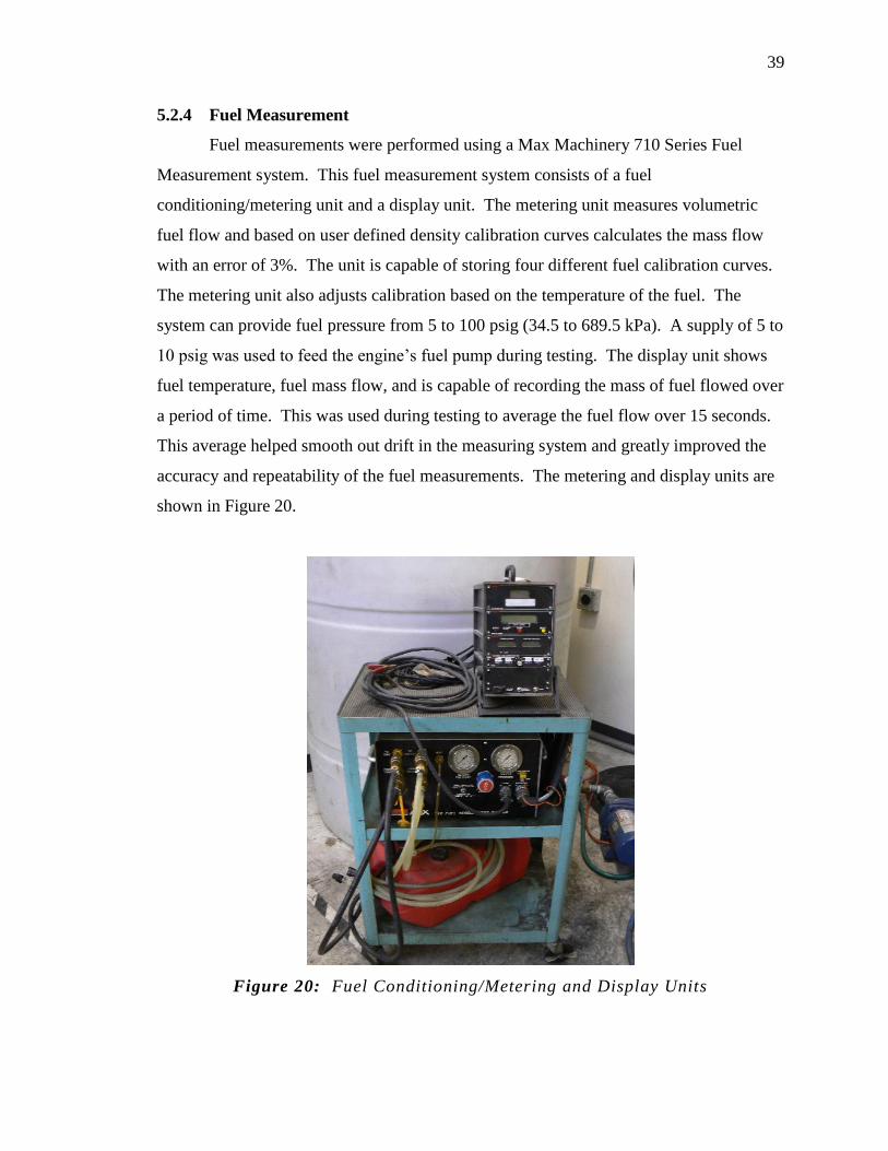
39

5.2.4 Fuel Measurement

Fuel measurements were performed using a Max Machinery 710 Series Fuel

Measurement system. This fuel measurement system consists of a fuel

conditioning/metering unit and a display unit. The metering unit measures volumetric

fuel flow and based on user defined density calibration curves calculates the mass flow

with an error of 3%. The unit is capable of storing four different fuel calibration curves.

The metering unit also adjusts calibration based on the temperature of the fuel. The

system can provide fuel pressure from 5 to 100 psig (34.5 to 689.5 kPa). A supply of 5 to

10 psig was used to feed the engine’s fuel pump during testing. The display unit shows

fuel temperature, fuel mass flow, and is capable of recording the mass of fuel flowed over

a period of time. This was used during testing to average the fuel flow over 15 seconds.

This average helped smooth out drift in the measuring system and greatly improved the

accuracy and repeatability of the fuel measurements. The metering and display units are

shown in Figure 20.

Figure 20: Fuel Conditioning/Metering and Display Units

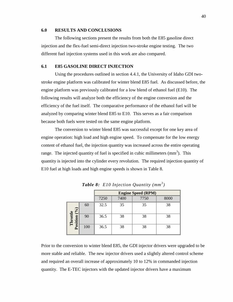
40

6.0 RESULTS AND CONCLUSIONS

The following sections present the results from both the E85 gasoline direct

injection and the flex-fuel semi-direct injection two-stroke engine testing. The two

different fuel injection systems used in this work are also compared.

6.1 E85 GASOLINE DIRECT INJECTION

Using the procedures outlined in section 4.4.1, the University of Idaho GDI two-

stroke engine platform was calibrated for winter blend E85 fuel. As discussed before, the

engine platform was previously calibrated for a low blend of ethanol fuel (E10). The

following results will analyze both the efficiency of the engine conversion and the

efficiency of the fuel itself. The comparative performance of the ethanol fuel will be

analyzed by comparing winter blend E85 to E10. This serves as a fair comparison

because both fuels were tested on the same engine platform.

The conversion to winter blend E85 was successful except for one key area of

engine operation: high load and high engine speed. To compensate for the low energy

content of ethanol fuel, the injection quantity was increased across the entire operating

range. The injected quantity of fuel is specified in cubic millimeters (mm3). This

quantity is injected into the cylinder every revolution. The required injection quantity of

E10 fuel at high loads and high engine speeds is shown in Table 8.

Table 8: E10 Injection Quantity (mm3)

Engine Speed (RPM)

7250 7400 7750 8000

Th

rott

le

Po

siti

on

(%

)

60 32.5 35 35 38

90 36.5 38 38 38

100 36.5 38 38 38

Prior to the conversion to winter blend E85, the GDI injector drivers were upgraded to be

more stable and reliable. The new injector drivers used a slightly altered control scheme

and required an overall increase of approximately 10 to 12% in commanded injection

quantity. The E-TEC injectors with the updated injector drivers have a maximum

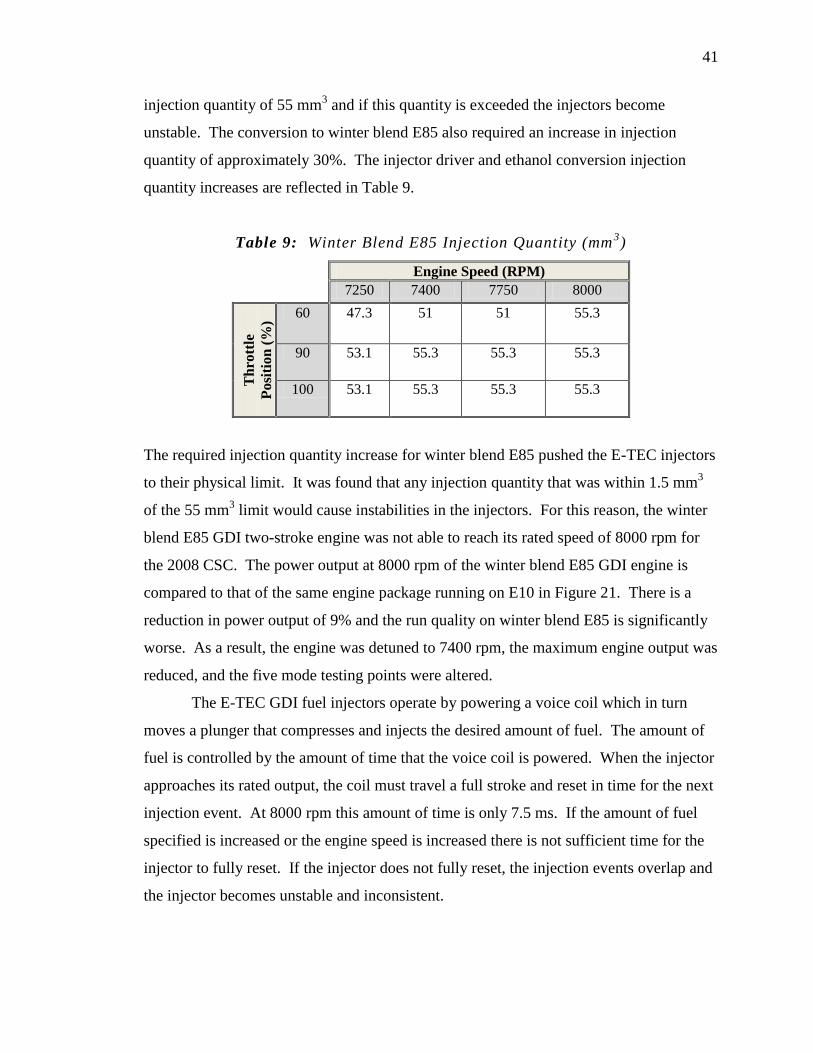
41

injection quantity of 55 mm3 and if this quantity is exceeded the injectors become

unstable. The conversion to winter blend E85 also required an increase in injection

quantity of approximately 30%. The injector driver and ethanol conversion injection

quantity increases are reflected in Table 9.

Table 9: Winter Blend E85 Injection Quantity (mm3)

Engine Speed (RPM)

7250 7400 7750 8000

Th

rott

le

Posi

tio

n (

%)

60 47.3 51 51 55.3

90 53.1 55.3 55.3 55.3

100 53.1 55.3 55.3 55.3

The required injection quantity increase for winter blend E85 pushed the E-TEC injectors

to their physical limit. It was found that any injection quantity that was within 1.5 mm3

of the 55 mm3 limit would cause instabilities in the injectors. For this reason, the winter

blend E85 GDI two-stroke engine was not able to reach its rated speed of 8000 rpm for

the 2008 CSC. The power output at 8000 rpm of the winter blend E85 GDI engine is

compared to that of the same engine package running on E10 in Figure 21. There is a

reduction in power output of 9% and the run quality on winter blend E85 is significantly

worse. As a result, the engine was detuned to 7400 rpm, the maximum engine output was

reduced, and the five mode testing points were altered.

The E-TEC GDI fuel injectors operate by powering a voice coil which in turn

moves a plunger that compresses and injects the desired amount of fuel. The amount of

fuel is controlled by the amount of time that the voice coil is powered. When the injector

approaches its rated output, the coil must travel a full stroke and reset in time for the next

injection event. At 8000 rpm this amount of time is only 7.5 ms. If the amount of fuel

specified is increased or the engine speed is increased there is not sufficient time for the

injector to fully reset. If the injector does not fully reset, the injection events overlap and

the injector becomes unstable and inconsistent.

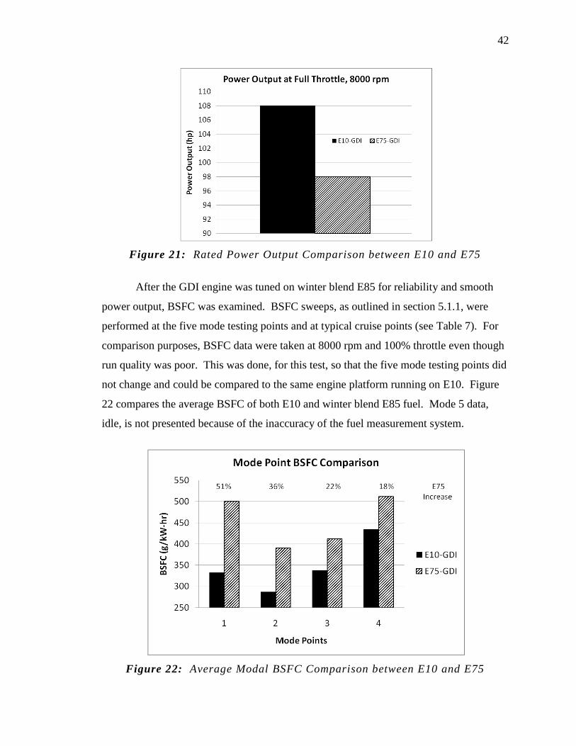
42

Figure 21: Rated Power Output Comparison between E10 and E75

After the GDI engine was tuned on winter blend E85 for reliability and smooth

power output, BSFC was examined. BSFC sweeps, as outlined in section 5.1.1, were

performed at the five mode testing points and at typical cruise points (see Table 7). For

comparison purposes, BSFC data were taken at 8000 rpm and 100% throttle even though

run quality was poor. This was done, for this test, so that the five mode testing points did

not change and could be compared to the same engine platform running on E10. Figure

22 compares the average BSFC of both E10 and winter blend E85 fuel. Mode 5 data,

idle, is not presented because of the inaccuracy of the fuel measurement system.

Figure 22: Average Modal BSFC Comparison between E10 and E75

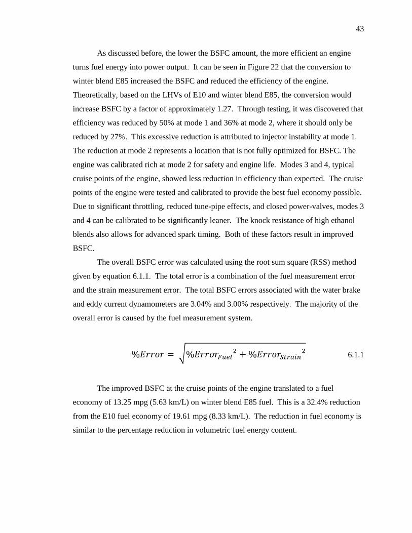
43

As discussed before, the lower the BSFC amount, the more efficient an engine

turns fuel energy into power output. It can be seen in Figure 22 that the conversion to

winter blend E85 increased the BSFC and reduced the efficiency of the engine.

Theoretically, based on the LHVs of E10 and winter blend E85, the conversion would

increase BSFC by a factor of approximately 1.27. Through testing, it was discovered that

efficiency was reduced by 50% at mode 1 and 36% at mode 2, where it should only be

reduced by 27%. This excessive reduction is attributed to injector instability at mode 1.

The reduction at mode 2 represents a location that is not fully optimized for BSFC. The

engine was calibrated rich at mode 2 for safety and engine life. Modes 3 and 4, typical

cruise points of the engine, showed less reduction in efficiency than expected. The cruise

points of the engine were tested and calibrated to provide the best fuel economy possible.

Due to significant throttling, reduced tune-pipe effects, and closed power-valves, modes 3

and 4 can be calibrated to be significantly leaner. The knock resistance of high ethanol

blends also allows for advanced spark timing. Both of these factors result in improved

BSFC.

The overall BSFC error was calculated using the root sum square (RSS) method

given by equation 6.1.1. The total error is a combination of the fuel measurement error

and the strain measurement error. The total BSFC errors associated with the water brake

and eddy current dynamometers are 3.04% and 3.00% respectively. The majority of the

overall error is caused by the fuel measurement system.

6.1.1

The improved BSFC at the cruise points of the engine translated to a fuel

economy of 13.25 mpg (5.63 km/L) on winter blend E85 fuel. This is a 32.4% reduction

from the E10 fuel economy of 19.61 mpg (8.33 km/L). The reduction in fuel economy is

similar to the percentage reduction in volumetric fuel energy content.

44

6.2 FLEX-FUEL SEMI-DIRECT INJECTION

The techniques described in section 4.4.2 were used to first perform a base E10

fuel calibration on the SDI two-stroke engine with the automotive engine control unit.

The engine package was then tested to determine the effect of fuel injection timing on the

engine. Sweeping the fuel injection timing at various calibration points did not

significantly affect the BSFC or power output of the engine. Sweeping injection timing

from 260° to 320° before top dead center (BTDC), the maximum variation in BSFC was

0.2% which is much less than the 3% error in the fuel measurement system (see section

5.2.4). BSFC was optimized on E10 fuel through adjustment of fuel quantity and ignition

timing.

Once the E10 base map was created, the flex-fuel compensation map was created

using the techniques described in section 4.4.2. The calibrated and calculated injection

quantity multipliers are shown in Figure 23. The calculated injection quantity multiplier

is based on the LHV of gasoline and ethanol. It can be seen in Figure 22 that the

calibrated injection quantity multiplier closely follows the calculated values from E10 to

E50. The higher blends of ethanol, above E50, were calibrated to be richer than the

calculated values. This was because the calculated injection multiplier value caused

severe after-burn in the tuned pipe. After-burn occurs when there is sufficient mixture

and energy to sustain combustion in the exhaust system of a two-stroke engine. To a

certain degree, after-burn can be used to reduce the hazardous emission production of an

engine. If it is too severe, it can lead to component failure and safety issues. The onset

of after-burn associated with high ethanol blends suggests poor injection timing and

reduced charge trapping. The larger fuel quantities require more injection time and

ideally the start of injection should be optimized. The SDI ECU did not allow for an

ethanol content compensation of injection timing, so a rich calibration strategy was used

to reduce combustion temperatures and reduce energy in the exhaust system to control

after-burn. The rich after-burn control strategy increases BSFC and reduces engine

efficiency.

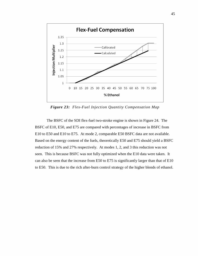
45

Figure 23: Flex-Fuel Injection Quantity Compensation Map

The BSFC of the SDI flex-fuel two-stroke engine is shown in Figure 24. The

BSFC of E10, E50, and E75 are compared with percentages of increase in BSFC from

E10 to E50 and E10 to E75. At mode 2, comparable E50 BSFC data are not available.

Based on the energy content of the fuels, theoretically E50 and E75 should yield a BSFC

reduction of 15% and 27% respectively. At modes 1, 2, and 3 this reduction was not

seen. This is because BSFC was not fully optimized when the E10 data were taken. It

can also be seen that the increase from E50 to E75 is significantly larger than that of E10

to E50. This is due to the rich after-burn control strategy of the higher blends of ethanol.

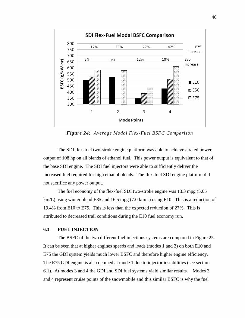
46

Figure 24: Average Modal Flex-Fuel BSFC Comparison

The SDI flex-fuel two-stroke engine platform was able to achieve a rated power

output of 108 hp on all blends of ethanol fuel. This power output is equivalent to that of

the base SDI engine. The SDI fuel injectors were able to sufficiently deliver the

increased fuel required for high ethanol blends. The flex-fuel SDI engine platform did

not sacrifice any power output.

The fuel economy of the flex-fuel SDI two-stroke engine was 13.3 mpg (5.65

km/L) using winter blend E85 and 16.5 mpg (7.0 km/L) using E10. This is a reduction of

19.4% from E10 to E75. This is less than the expected reduction of 27%. This is

attributed to decreased trail conditions during the E10 fuel economy run.

6.3 FUEL INJECTION

The BSFC of the two different fuel injections systems are compared in Figure 25.

It can be seen that at higher engines speeds and loads (modes 1 and 2) on both E10 and

E75 the GDI system yields much lower BSFC and therefore higher engine efficiency.

The E75 GDI engine is also detuned at mode 1 due to injector instabilities (see section

6.1). At modes 3 and 4 the GDI and SDI fuel systems yield similar results. Modes 3

and 4 represent cruise points of the snowmobile and this similar BSFC is why the fuel

47

economy of the SDI is close to that of the GDI. At all mode points the GDI proves to be

more efficient than the SDI on E75. This is partially because the GDI system was

optimized for one particular fuel at a time where the SDI system was designed to work

with any ethanol blend. Overall, the GDI fuel injection system offers more precise fuel

control, reduced short-circuiting, and improved combustion efficiency.

Figure 25: GDI and SDI Fuel System BSFC Comparison

6.4 CONCLUSIONS

The main goal of the research presented in this thesis was to explore the necessary

engine modifications and calibration strategies to efficiently combust blended ethanol

fuels in fuel injected two-stroke engines. The second goal was to explore the use and

effects of ethanol as a fuel source. Both the winter blend E85 and flex-fuel systems

proved to be successful.

The GDI winter blend E85 ethanol system yielded BSFC performance that was

close to that expected from the lower energy content of ethanol. A fuel economy of 13.3

mpg (5.65 km/L) was achieved with winter blend E85. Maximum power output and

mode 1 BSFC values could be improved with injectors that could handle the necessary

48

increase in fuel quantity associated with winter blend E85 fuel. The cold start

characteristics of the GDI engine were very satisfactory. Overall, the GDI system proved

to have decent performance, good fuel economy, and high fuel efficiency. At the 2008

CSC, the University of Idaho placed second overall and was awarded best acceleration

and quietest snowmobile running the GDI winter blend E85 engine platform [38].

The flex-fuel SDI system functioned properly and yielded good performance on

all ethanol blends. The BSFC of the engine package was close to that calculated based

on the low energy content of ethanol. Fuel economies of 13.3 (5.65 km/L) and 16.5 mpg

(7.0 km/L) were achieved using E75 and E10 fuel respectively. Satisfactory cold start

characteristics were obtained. The flex-fuel system provided ethanol content feedback

that controlled compensation maps for injection quantity and ignition timing. It was

found that fuel injection timing needed to be adjusted based on ethanol content. If this

parameter were incorporated, engine efficiency while on high ethanol blends could be

improved. At the 2009 CSC, the University of Idaho flex-fuel SDI snowmobile placed

third overall and was also awarded best fuel economy and best acceleration [39].

Blended ethanol fuels have different physical properties and environmental

impacts than gasoline. Blended ethanol fuels have a lower energy content, more

corrosive nature, higher latent heat, limited shelf life, higher knock resistance, and

dissimilar emissions. If the higher knock resistance is not utilized, the lower energy

content results in reduced engine efficiency and fuel economy. The corrosive nature of

ethanol fuels requires modifications to the entire fuel system. The increased latent heat

of ethanol fuels reduces an engine’s cold start ability. Blended ethanol fuels produce less

CO and UHC emissions but also produce more NOx, ethanol, acetaldehyde, and

formaldehyde emissions.

This research proves that fuel injected two-stroke engines can be converted for the

use of blended ethanol fuels. Both engine platforms showed a reduction in efficiency

similar to that inherent of blended ethanol fuels. Both engine platforms achieved good

performance and high power-to-weight ratios. As predicted, the GDI fuel injection

system proved to be more efficient than the SDI system. Without proper emission testing

equipment the emission production of the fuel injection systems and the fuel can only be

theorized. As a fuel, ethanol offers both drawbacks and advantages.

49

7.0 RECOMMENDATIONS AND FUTURE WORK

The following are recommendations for future engine research and design at the

University of Idaho. The following topics are deserving of further investigation.

7.1 INCREASED/VARIABLE COMPRESSION

Future blended ethanol fueled engines should be designed to take advantage of the

high knock resistance of ethanol. There are two different ways of taking advantage of the

high octane rating of ethanol. The first is increasing geometric compression ratio through

reducing the clearance volume. The second is increasing the density of trapped air

through forced induction. Both methods increase combustion efficiency, which then

improves performance and fuel economy. Fully taking advantage of ethanol’s high

knock resistance partially mitigates its low energy content.

It is relatively simple to increase the compression ratio for an engine that is

designed for one blend of ethanol fuel. The addition of a turbocharger with a set amount

of boost is also possible (see Nathan Bradbury’s thesis [20]). The application of these

methods to a flex-fuel engine is more complex. The variation in ethanol blends requires

either variable compression or variable boost. Variable compression ratio requires a

cylinder head with the ability to change its trapped volume. Variable boost requires an

electronic waste-gate that is controlled by the ECU to adjust the amount of boost

according to the blend of ethanol fuel.

7.2 HIGH-PRESSURE DIRECT INJECTION

High-Pressure Direct Injection (HPDI) injects fuel directly into the combustion

chamber at pressures exceeding 1000 psi. Typical HPDI systems utilize a mechanical

high-pressure fuel pump, a common fuel rail, and automotive high-pressure injectors.

The E-TEC GDI system is only capable of injection pressures of 550-600 psi. This

increase in pressure would substantially increase the stratified combustion efficiency,

improve vaporization, and reduce the time required for injection. With HPDI there is the

possibility of utilizing stratified combustion during cruise for substantially better fuel

economy. For more information on stratified cruise see Justin Johnson’s thesis [12]. The

reduction in required injection time results in more precise fuel control and improved

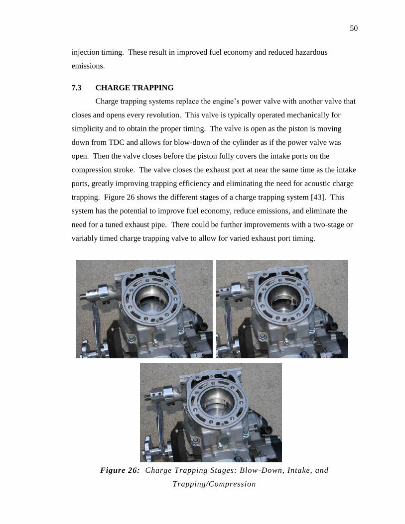
50

injection timing. These result in improved fuel economy and reduced hazardous

emissions.

7.3 CHARGE TRAPPING

Charge trapping systems replace the engine’s power valve with another valve that

closes and opens every revolution. This valve is typically operated mechanically for

simplicity and to obtain the proper timing. The valve is open as the piston is moving

down from TDC and allows for blow-down of the cylinder as if the power valve was

open. Then the valve closes before the piston fully covers the intake ports on the

compression stroke. The valve closes the exhaust port at near the same time as the intake

ports, greatly improving trapping efficiency and eliminating the need for acoustic charge

trapping. Figure 26 shows the different stages of a charge trapping system [43]. This

system has the potential to improve fuel economy, reduce emissions, and eliminate the

need for a tuned exhaust pipe. There could be further improvements with a two-stage or

variably timed charge trapping valve to allow for varied exhaust port timing.

Figure 26: Charge Trapping Stages: Blow-Down, Intake, and

Trapping/Compression

51

7.4 TESTING EQUIPMENT

The research presented in this thesis provides a good baseline of blended ethanol

fuel data. The data and results of this research could be improved with higher quality

testing equipment. Before further engine research and development is conducted at the

University of Idaho, the engine testing equipment needs to be upgraded. A fuel

measuring system with an accuracy of +/- 2% of actual flow is necessary. An emission

analyzer capable of continuously reading emissions from an un-calibrated engine for up

to 10 minutes would increase engine calibration efficiency and provide more meaningful

results. In-cylinder pressure data with combustion analyzer would also reduce calibration

time and improve combustion analysis. Upgraded testing equipment would greatly

improve the quality of engine research and development at the University of Idaho.

52

BIBLIOGRAPHY

1. Walter, S.R., “Corn Ethanol as an Alternative Fuel: Technical and Economic

Issues,” SAE 2006-01-0179, 2006.

2. Society of Automotive Engineers, Inc., The SAE Clean Snowmobile Challenge

2009 Rules, SAE Inc., Warrendale, PA, 2008.

3. 69 Fed.Reg. 65,348 (Nov. 10, 2004).

4. Lela C.C., White J.J., “Laboratory Testing of Snowmobile Emissions,” Report

Number SwRI 08.05486, Southwest Research Institute, San Antonio, July 2002.

5. United States Department of the Interior National Park Service, Special

Regulations; Areas of the National Park System, Final Rule. 36 CFR Part 7,

November 10, 2004.

6. Society of Automotive Engineers, Inc., The SAE Clean Snowmobile Challenge

2008 Rules, SAE Inc., Warrendale, PA, 2007.

7. Strauss, S., Zeng, Y., Montgomery, D., “Optimization of the E-TEC™

Combustion System for Direct-Injection Two-Stroke Engines Toward 3-Star

Emissions,” SAE 2003-32-0007/20034307, 2003.

8. Bradbury, N., Schiermeier R., Harris, T., DenBraven, K., “University of Idaho’s

Clean Snowmobile Design Using a Direct-Injection Two-Stoke,” SAE 2005-01-

3680, 2005.

9. Bradbury, N., et al. “University of Idaho’s Clean Snowmobile Design Using a

Direct Injection Two-Stroke,” SAE 2006-32-0050, 2006.

10. Society of Automotive Engineers, Inc., The SAE Clean Snowmobile Challenge

Results, SAE Inc., Warrendale, PA, 2007.

11. Wright, C.W., White J.J., “Development and Validation of a Snowmobile Engine

Emission Test Procedure,” SAE 982017, Milwaukee, Wisconsin Sept. 1998.

12. Johnson, J., “Comparison of Stratified and Homogeneous Combustion in a Direct-

Injected Two-Stroke Engine for Snowmobile Applications,” M.S. Thesis,

University of Idaho, 2007.

13. Society of Automotive Engineers, Inc., The SAE Clean Snowmobile Challenge

Results, SAE Inc., Warrendale, PA, 2005.

14. Society of Automotive Engineers, Inc., The SAE Clean Snowmobile Challenge

Results, SAE Inc., Warrendale, PA, 2003.

53

15. Society of Automotive Engineers, Inc., The SAE Clean Snowmobile Challenge

Results, SAE Inc., Warrendale, PA, 2004.

16. Zhao F., Harrington H.L., Lai M., “Automotive Gasoline Direct-Injection

Engines,” Society of Automotive Engineers, Inc. Warrendale, PA. 2002.

17. Stone R. “Introduction to Internal Combustion Engines,” Antony Rowe Ltd.

Chippenham, Wiltshire, 1997.

18. Heywood J.B., “Internal Combustion Engine Fundamentals,” McGraw Hill, Inc.

1988.

19. Heywood, J., Sher, E., “The Two-Stroke Cycle Engine, Its Development,

Operation, and Design”, Taylor and Francis Inc., Braun-Braumfield, Ann Arbor,

MI. 1999.

20. Bradbury, N., “Retrofitting Direct-Injection and a Turbocharger to a Two-Stroke

Engine for Snowmobile Applications,” M.S. Thesis, University of Idaho, 2006.

21. Morikawa K., Takimoto H., Ogi T., “A Study of Direct Fuel Injection Two-Stroke

Engine for High Specific Power Output and High Engine Speed,” SAE Paper

1999-01-3288 / JSAE 9938043, 1999.

22. Strauss S., Zeng Y., “The Effect of Fuel Spray Momentum on Performance and

Emissions of Direct-Injected Two-Stroke Engines,” SAE Paper 2004-32-0013 /

JSAE 20044300, 2004.

23. Wasil J., Montgomery D., Strauss S., Bagley S.T., “Life Assessment of PM,

Gaseous Emissions, and Oil Usage in Modern Marine Outboard Engines,” SAE

Paper 2004-32-0092/20044379, 2004.

24. Blair G.P. “Design and Simulation of Two-Stroke Engines,” Society of

Automotive Engineers, Inc. Warrendale, Pa, 1996.

25. Zhao F., Harrington H.L., Lai M., “Automotive Gasoline Direct-Injection

Engines,” Society of Automotive Engineers, Inc. Warrendale, PA. 2002.

26. Yucesu, H.S., Topgul, T., Cinar, C., and Okur, M., “Effect of ethanol – gasoline

blends on engine performance and exhaust emissions in different compression

ratios,” Applied Thermal Engineering 26, Elsevier, pp. 2272-2278, 2006.

27. Niven, R.K., “Ethanol in gasoline: environmental impacts and sustainability

review article,” Renewable and Sustainable Energy Reviews 9, Elsevier, pp. 536-

555, 2005.

54

28. Furey, Robert L., “Volatility Characteristics of Gasoline-Alcohol and Gasoline-

Ether Fuel Blends,” SAE Paper 852116, 1985.

29. U.S. Department of Energy: Energy Efficiency and Renewable Energy,

Handbook for Handling, Storing, and Dispensing E85,

(http://afdc.energy.gov/afdc/pdfs/41853.pdf), April 3, 2009.

30. Varde, K., Jones, A., Knutsen, A., Mertz, D., and Yu, P., “Exhaust Emissions and

Energy Release Rates from a Controlled Spark Ignition Engine using Ethanol

Blends,” Automobile Engineering, IMechE, vol. 221, pp. 933-941, 2007.

31. U.S. Department of Energy Energy Efficiency and Renewable Energy,

Alternative Fuels and Advanced Vehicles Data Center,

(www.afdc.energy.gov/afdc/ethanol), April 3, 2009.

32. Chevron Corp., Longer Term Storage of Gasoline,

(www.chevron.com/products/ourfuels/

prodserv/fuels/technical_safety_bulletins/longterm_gasoline.aspx), April 3, 2009.

33. Miller, A., “Corn-fed Muscles,” Modern Metals, Trend Publishing, v 63, n 1, pp.

71-75, 2007.

34. Fuel and Oil Hoses. SAE standard J30, SAE Inc., Warrendale, PA.

35. Gao, J., Jiang, D., and Huang, Z., “Spray properties of alternative fuel: A

comparative analysis of ethanol – gasoline blends and gasoline,” Fuel 86,

Elsevier, pp. 1645-1650, 2007.

36. Celik, M.B., “Experimental determination of suitable ethanol – gasoline blend

rate at high compression ratio for gasoline engine,” Applied Thermal Engineering

2007.10.028, 2007.

37. Continental Corp., Flex Fuel Sensor,

(usa.vdo.com/products_solutions/cars/powertrain/ sensors/powertrain/flex-fuel-

sensor/flex-fuel-sensor.htm), April 3, 2009.

38. Society of Automotive Engineers, Inc., The SAE Clean Snowmobile Challenge

Results, SAE Inc., Warrendale, PA, 2008.

39. Society of Automotive Engineers, Inc., The SAE Clean Snowmobile Challenge

Results, SAE Inc., Warrendale, PA, 2009.

40. Land and Sea, Inc., DynoMiteTM

Snowmobile Dyno #075-200-1K Specs,

(www.land-and-sea.com/snowmobile-dyno/DYNOmite%20Snow%20075-200-

1K%20Quick Specs.pdf), April 3, 2009.

55

41. Borghi & Saveri SRL, “Eddy Current Dynamometers Instruction Manual,”

Bologna, Italy, 1998.

42. Interface Force Measurments Ltd., Model SSM Series,

(www.interface.uk.com/pdf/2000/ ssm.pdf), April 6, 2009.

43. Zeppelin, S., “Clean Two-Stroke Engines – Boyesen Reinvents the Two-Stroke,”

MaxSled, Sept. 2008.

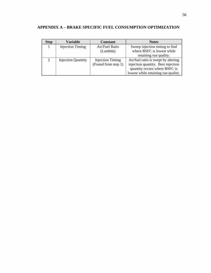
56

APPENDIX A – BRAKE SPECIFIC FUEL CONSUMPTION OPTIMIZATION

Step Variable Constant Notes

1 Injection Timing Air/Fuel Ratio

(Lambda)

Sweep injection timing to find

where BSFC is lowest while

retaining run quality.

2 Injection Quantity Injection Timing

(Found from step 1)

Air/fuel ratio is swept by altering

injection quantity. Best injection

quantity occurs where BSFC is

lowest while retaining run quality.