1

Example Application 19

Swelling of a Fully Wetted Slope

2

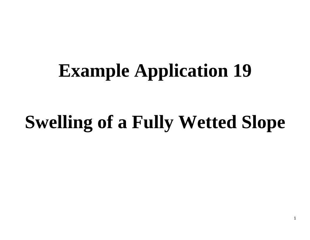
Soil Properties for Slope

Soil 3 4 5

mass density (kg/m3) 1728.3 1575.4 1978.5

bulk modulus (Pa) 1.54x107 3.27x107 2.93x107

shear modulus (Pa) 7.12x106 1.5x107 2.2x107

cohesion (Pa) 4,800 4,800 1,440

friction angle (degrees)

30 30 40

tension limit (Pa) 0.0 0.0 0.0

swelling properties

a1 1.533 0.694 0.0004

a3 0.436 0.468 0.00047

c1 -0.0187 -0.0211 0

c3 -0.0215 -0.023 0.001

angle 0 0 0

m1 0.023 0.028 0

m3 0.036 0.036 0

modnum 1 1 2

ninc 50,000 50,000 50,000

pressure 1.0133x105 1.0133x105 1.0133x105

3

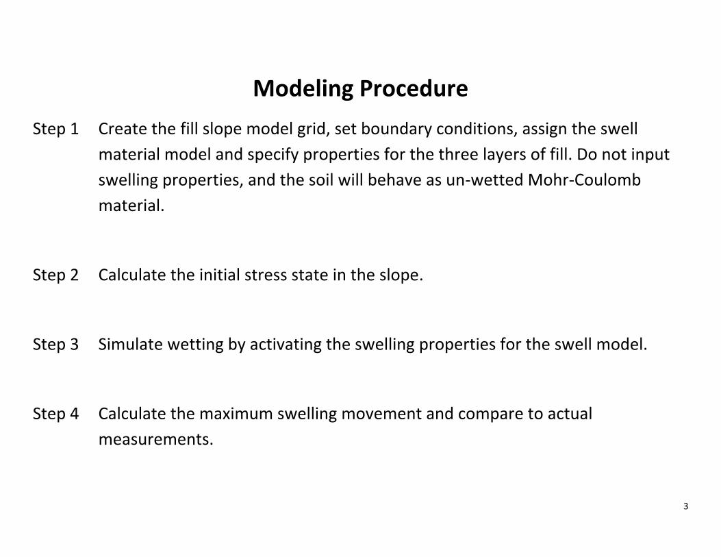
Modeling Procedure

Step 1 Create the fill slope model grid, set boundary conditions, assign the swell

material model and specify properties for the three layers of fill. Do not input

swelling properties, and the soil will behave as un-wetted Mohr-Coulomb

material.

Step 2 Calculate the initial stress state in the slope.

Step 3 Simulate wetting by activating the swelling properties for the swell model.

Step 4 Calculate the maximum swelling movement and compare to actual

measurements.

4

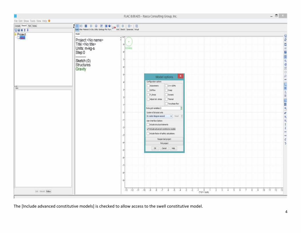
The [Include advanced constitutive models] is checked to allow access to the swell constitutive model.

5

A project title is assigned, and a project file wetslope.prj is created and stored in a working directory.

6

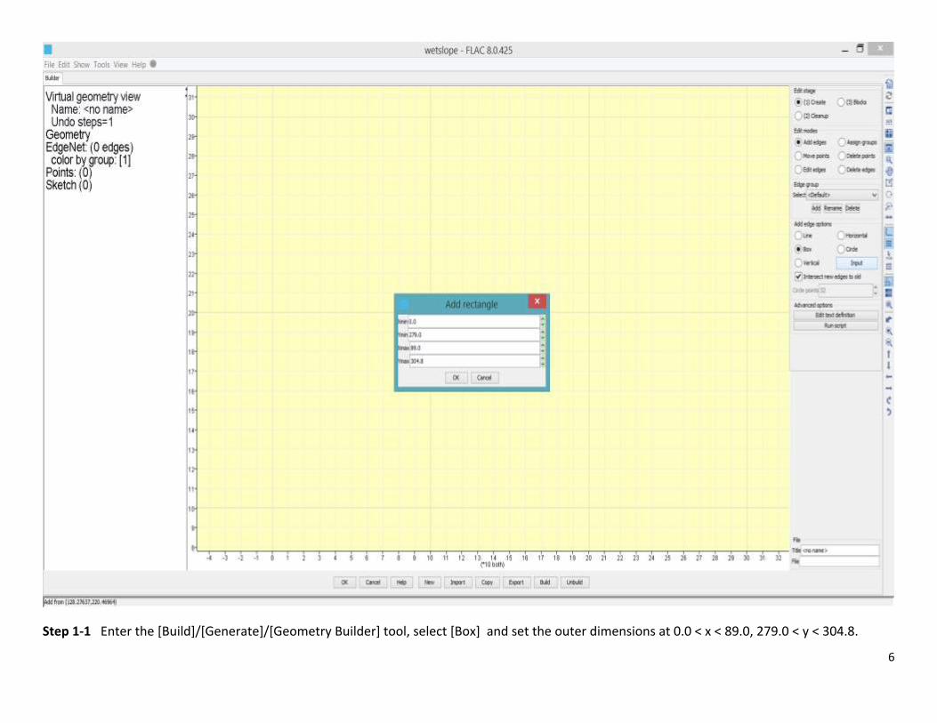
Step 1-1 Enter the [Build]/[Generate]/[Geometry Builder] tool, select [Box] and set the outer dimensions at 0.0 < x < 89.0, 279.0 < y < 304.8.

7

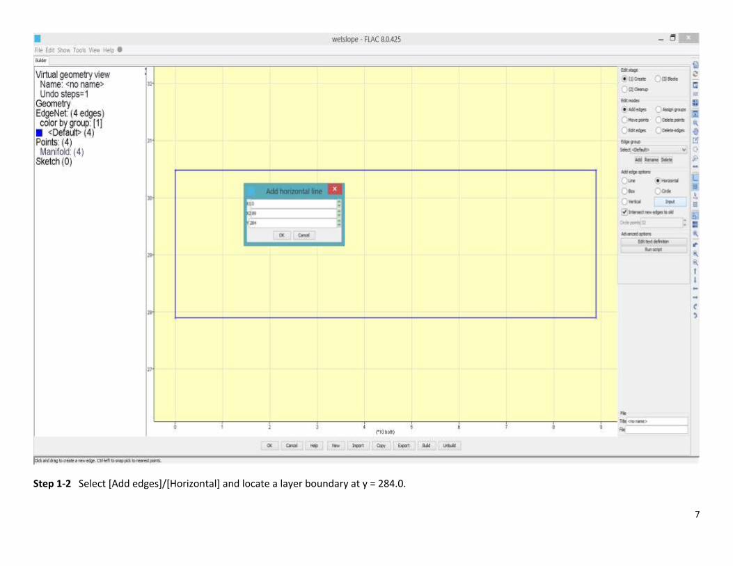
Step 1-2 Select [Add edges]/[Horizontal] and locate a layer boundary at y = 284.0.

8

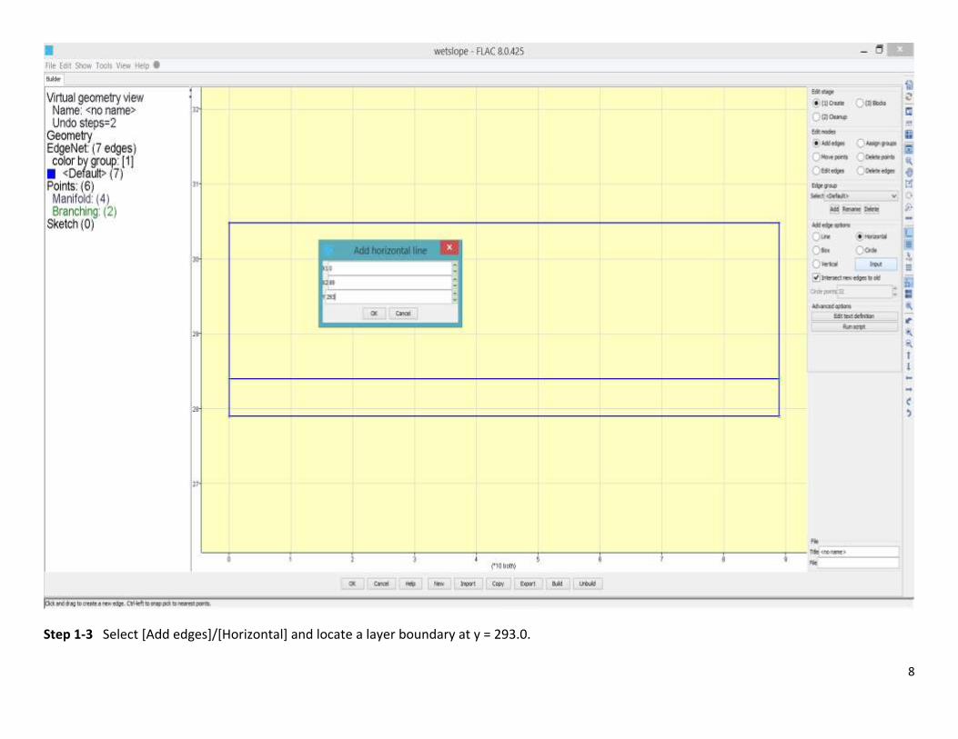
Step 1-3 Select [Add edges]/[Horizontal] and locate a layer boundary at y = 293.0.

9

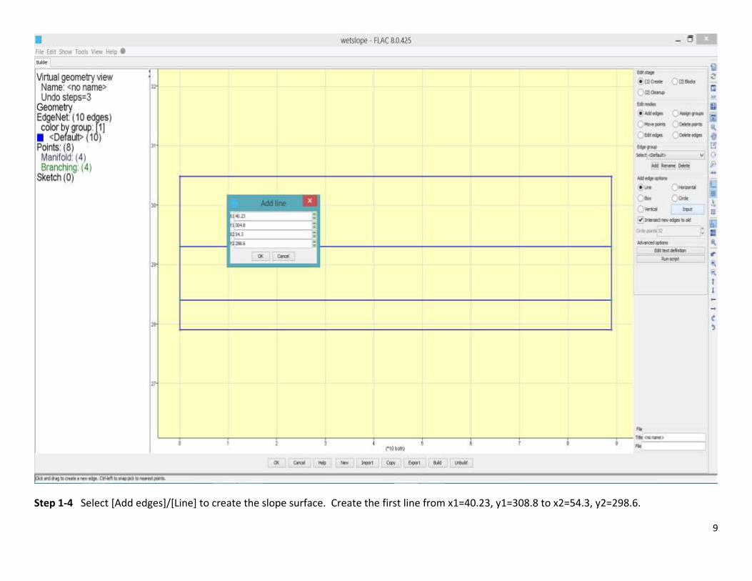
Step 1-4 Select [Add edges]/[Line] to create the slope surface. Create the first line from x1=40.23, y1=308.8 to x2=54.3, y2=298.6.

10

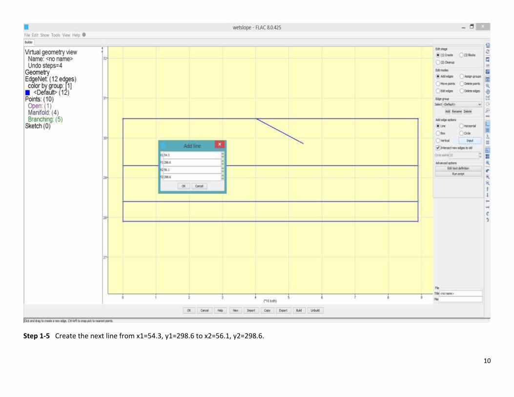
Step 1-5 Create the next line from x1=54.3, y1=298.6 to x2=56.1, y2=298.6.

11

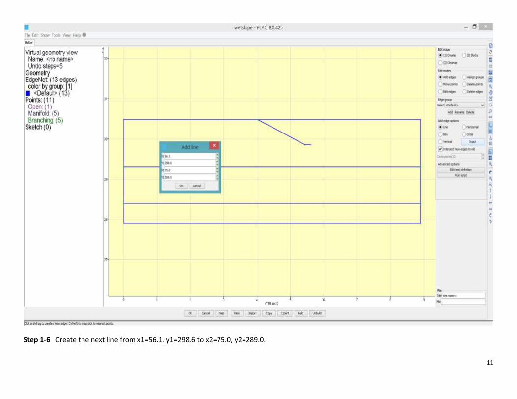
Step 1-6 Create the next line from x1=56.1, y1=298.6 to x2=75.0, y2=289.0.

12

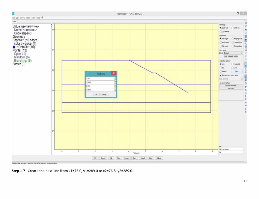
Step 1-7 Create the next line from x1=75.0, y1=289.0 to x2=76.8, y2=289.0.

13

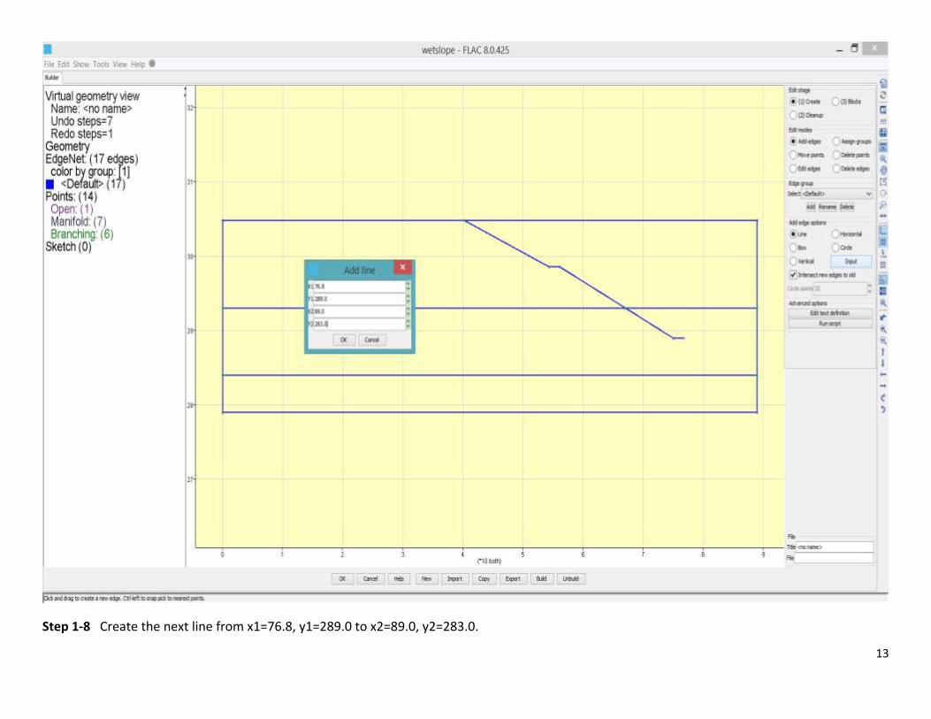
Step 1-8 Create the next line from x1=76.8, y1=289.0 to x2=89.0, y2=283.0.

14

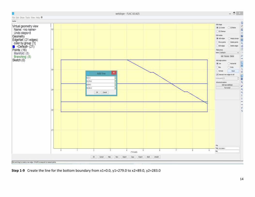
Step 1-9 Create the line for the bottom boundary from x1=0.0, y1=279.0 to x2=89.0, y2=283.0

15

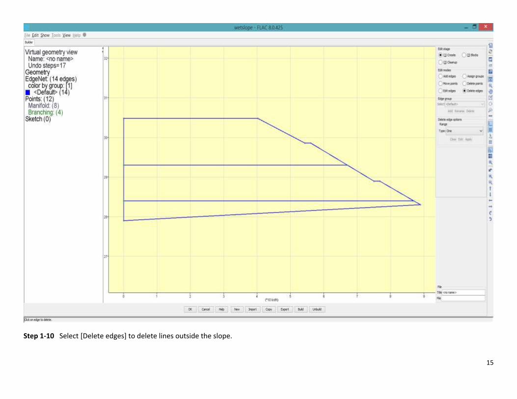
Step 1-10 Select [Delete edges] to delete lines outside the slope.

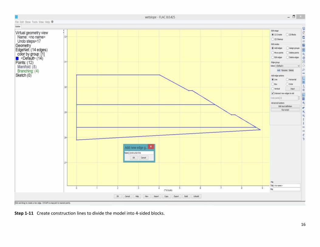
16

Step 1-11 Create construction lines to divide the model into 4-sided blocks.

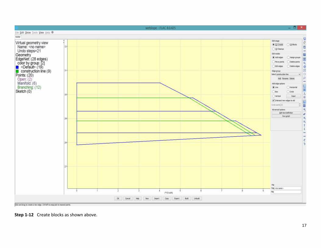
17

Step 1-12 Create blocks as shown above.

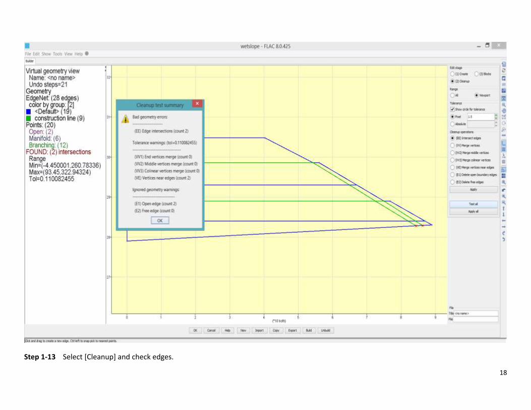
18

Step 1-13 Select [Cleanup] and check edges.

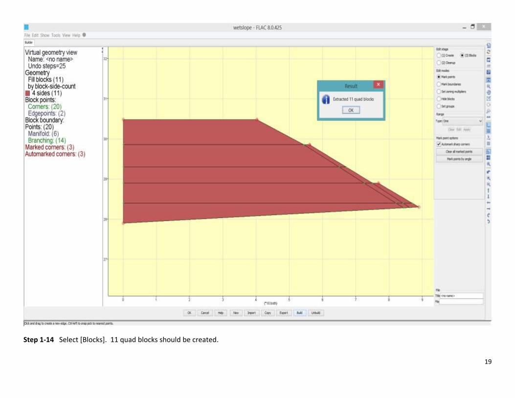
19

Step 1-14 Select [Blocks]. 11 quad blocks should be created.

20

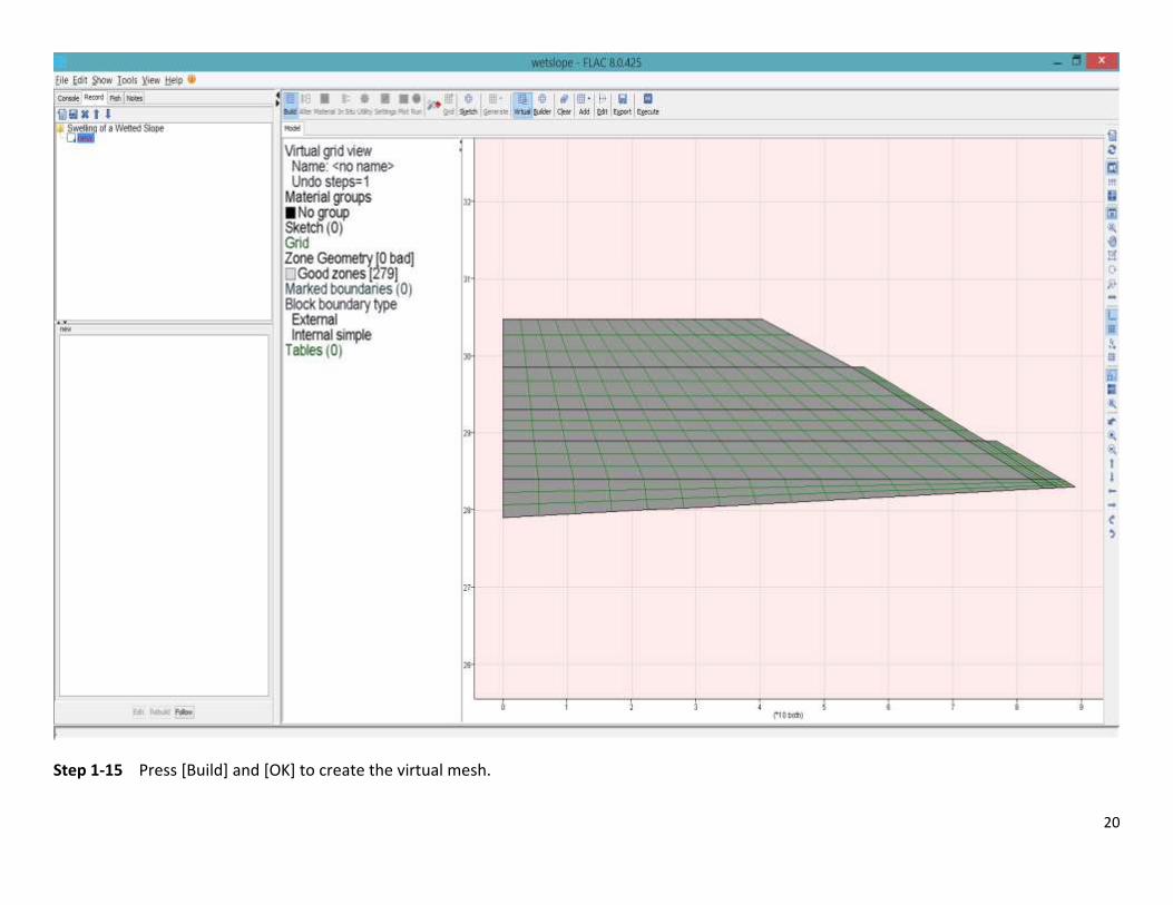
Step 1-15 Press [Build] and [OK] to create the virtual mesh.

21

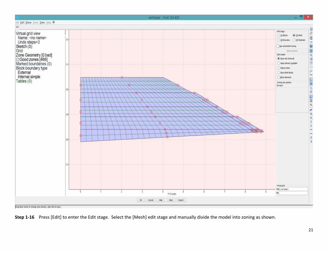
Step 1-16 Press [Edit] to enter the Edit stage. Select the [Mesh] edit stage and manually divide the model into zoning as shown.

22

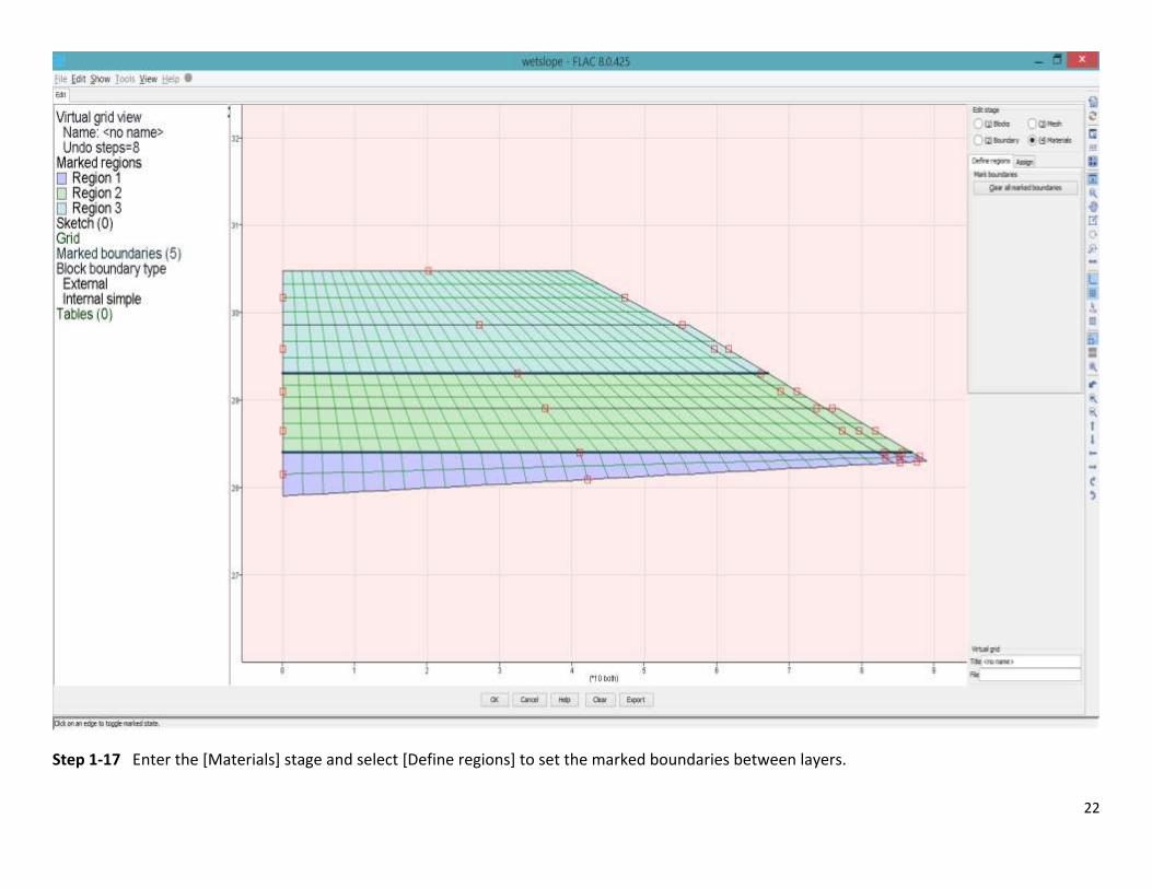
Step 1-17 Enter the [Materials] stage and select [Define regions] to set the marked boundaries between layers.

23

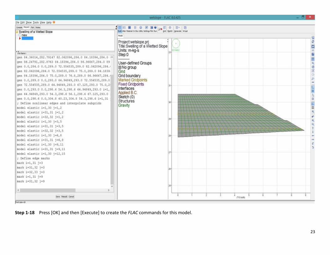
Step 1-18 Press [OK] and then [Execute] to create the FLAC commands for this model.

24

Step 1-19 Enter the [Material]/[Model], select [Region] range, specify the group name Soil3 and select the [swell] plastic model. Click the mouse

on a zone inside the Soil3 layer to open the Model swell properties dialog. Input the elastic and plastic properties. Leave the swelling properties

blank, and the initial behavior will be a Mohr-Coulomb material. Press [OK] to create the FLAC command.

25

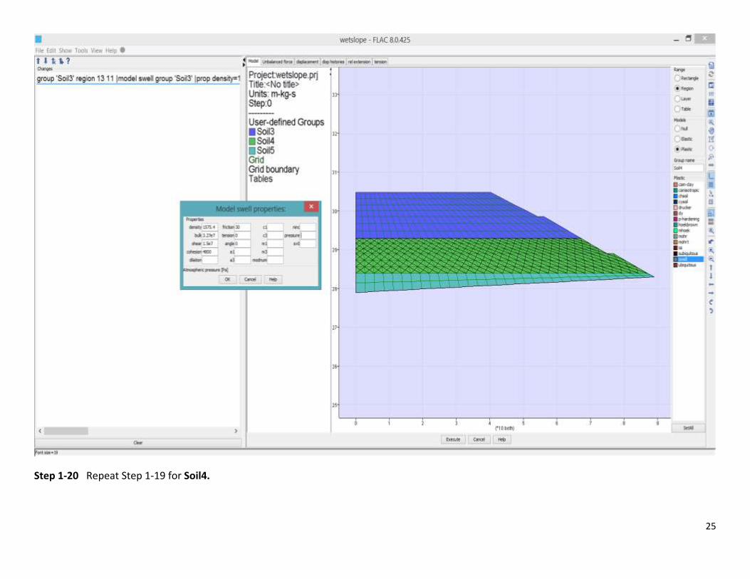
Step 1-20 Repeat Step 1-19 for Soil4.

26

Step 1-21 Repeat Step 1-19 for Soil5. Press [Execute] to send these commands to FLAC.

27

Step 1-22 Enter [In Situ]/[Fix], select [Fix]/[X] and drag the mounse along the left boundary to fix the boundary in the x-direction. Select

[Fix]/[X&Y] and drag the mouse along the bottom boundary to fix the boundary in both x- and y-directions.

28

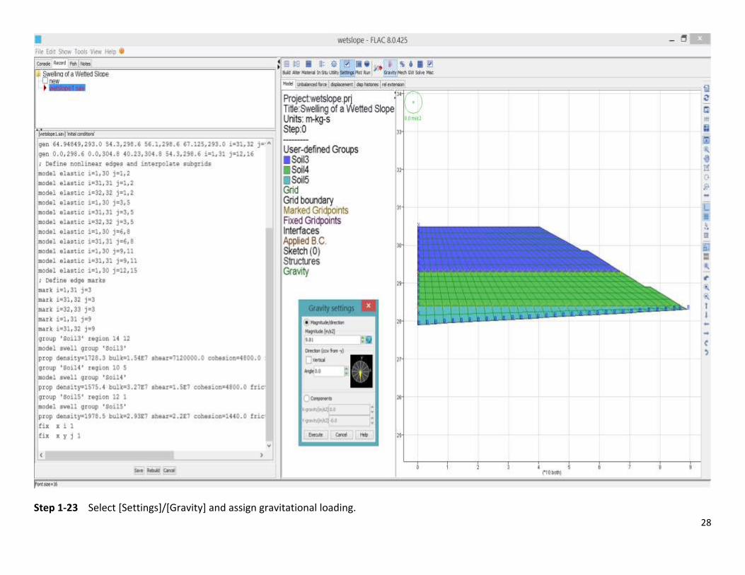
Step 1-23 Select [Settings]/[Gravity] and assign gravitational loading.

29

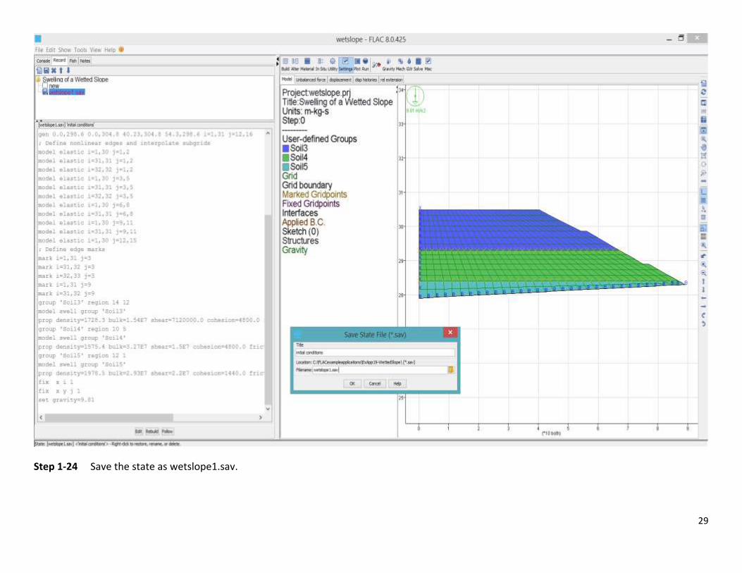
Step 1-24 Save the state as wetslope1.sav.

30

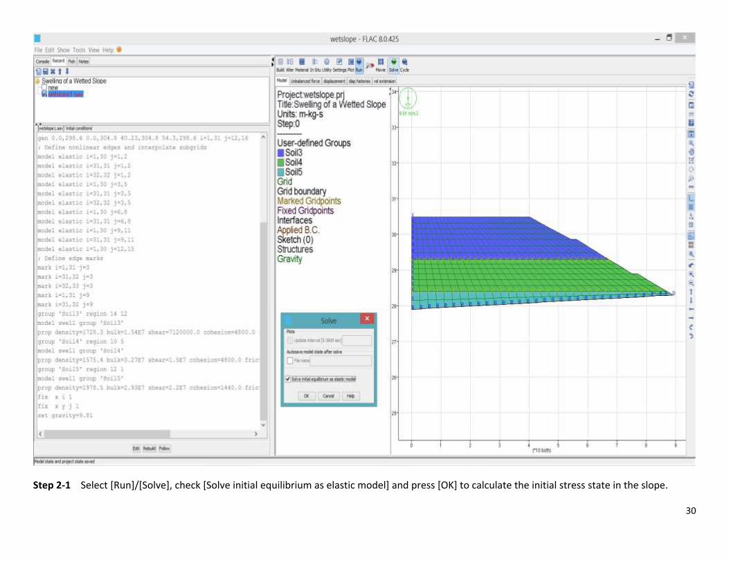
Step 2-1 Select [Run]/[Solve], check [Solve initial equilibrium as elastic model] and press [OK] to calculate the initial stress state in the slope.

31

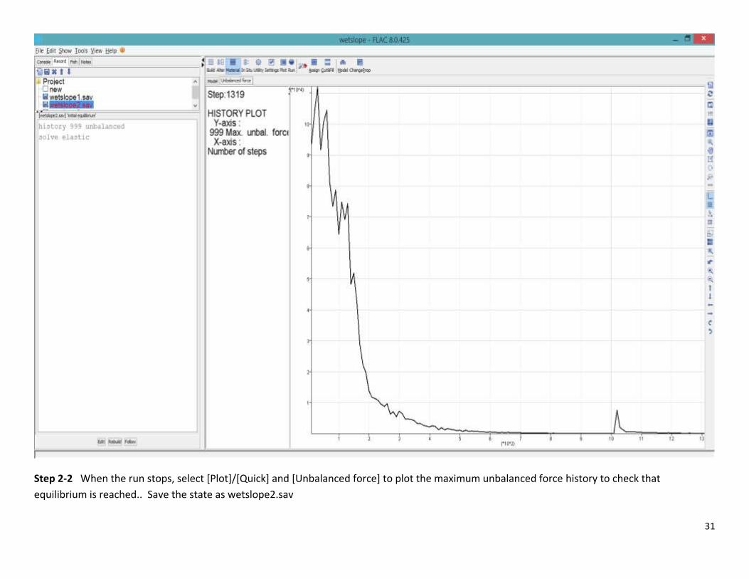
Step 2-2 When the run stops, select [Plot]/[Quick] and [Unbalanced force] to plot the maximum unbalanced force history to check that

equilibrium is reached.. Save the state as wetslope2.sav

32

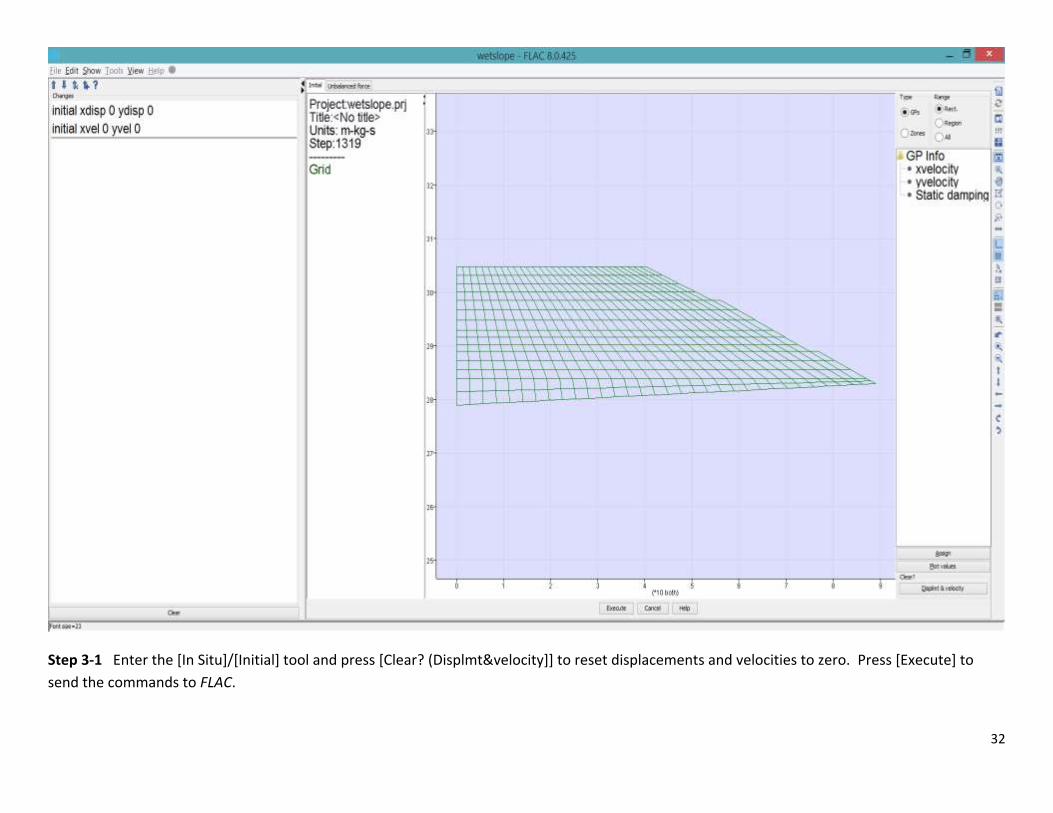
Step 3-1 Enter the [In Situ]/[Initial] tool and press [Clear? (Displmt&velocity]] to reset displacements and velocities to zero. Press [Execute] to

send the commands to FLAC.

33

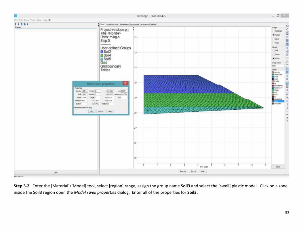
Step 3-2 Enter the [Material]/[Model] tool, select [region] range, assign the group name Soil3 and select the [swell] plastic model. Click on a zone

inside the Soil3 region open the Model swell properties dialog. Enter all of the properties for Soil3.

34

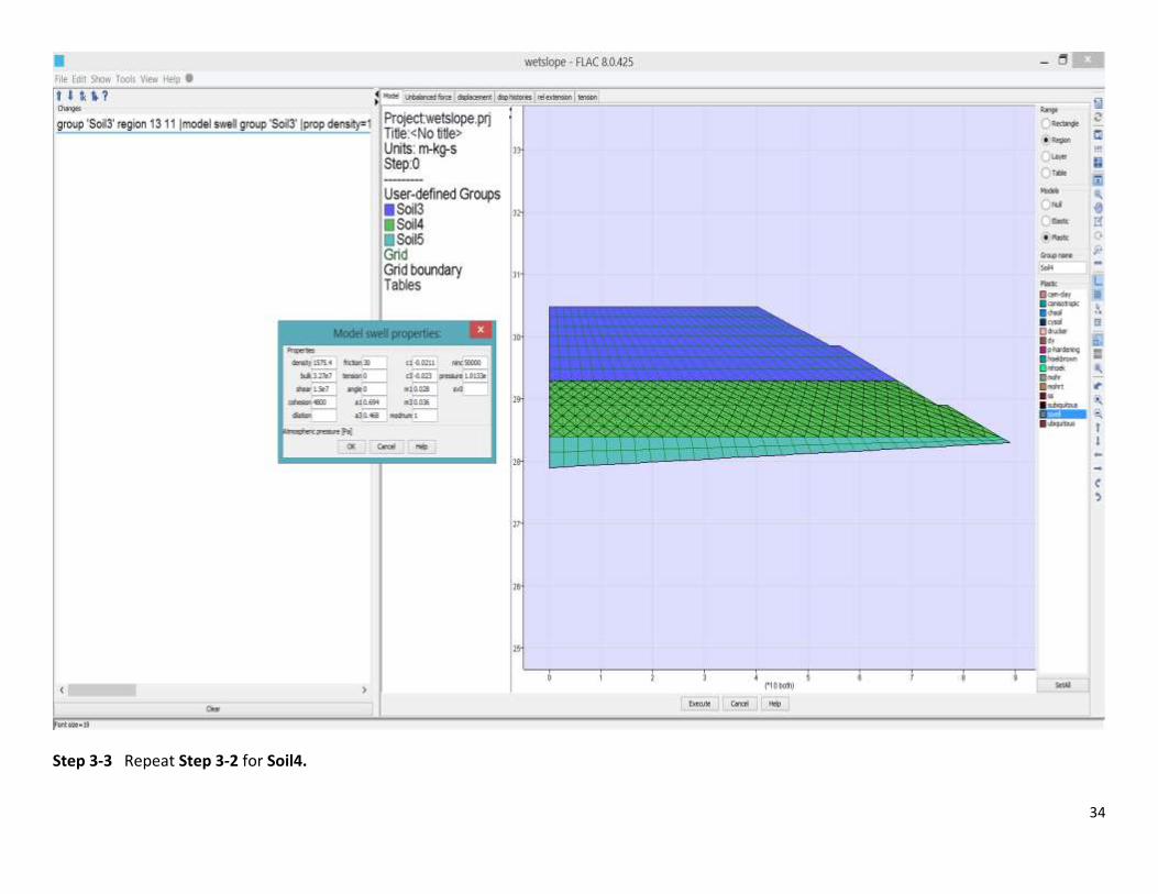
Step 3-3 Repeat Step 3-2 for Soil4.

35

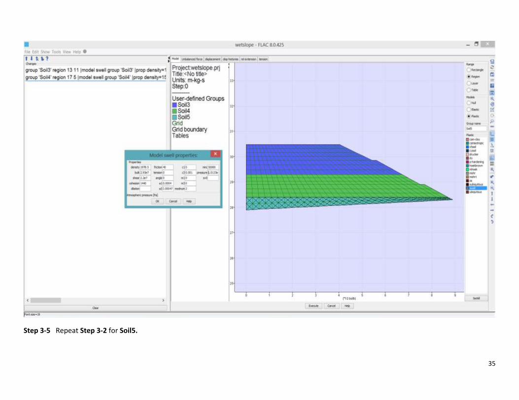
Step 3-5 Repeat Step 3-2 for Soil5.

36

Step 3-6 Monitor the x- and y-displacement at the slope crest in the [Utility]/[History] tool.

37

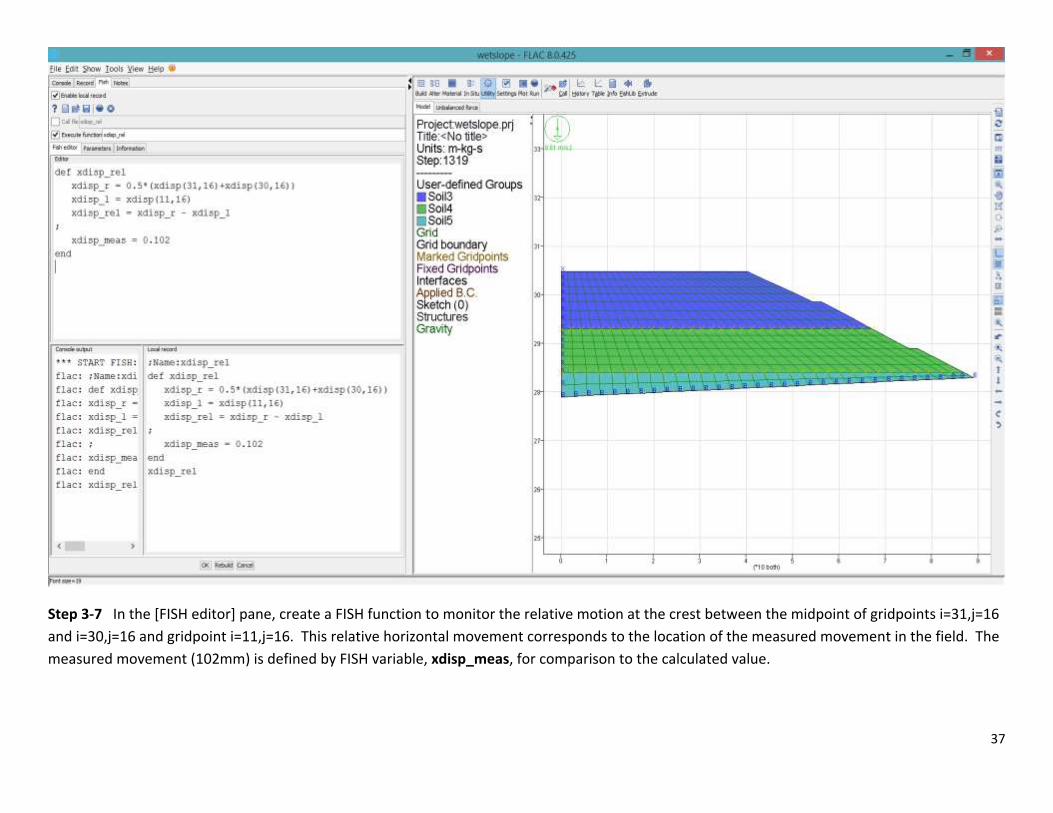
Step 3-7 In the [FISH editor] pane, create a FISH function to monitor the relative motion at the crest between the midpoint of gridpoints i=31,j=16

and i=30,j=16 and gridpoint i=11,j=16. This relative horizontal movement corresponds to the location of the measured movement in the field. The

measured movement (102mm) is defined by FISH variable, xdisp_meas, for comparison to the calculated value.

38

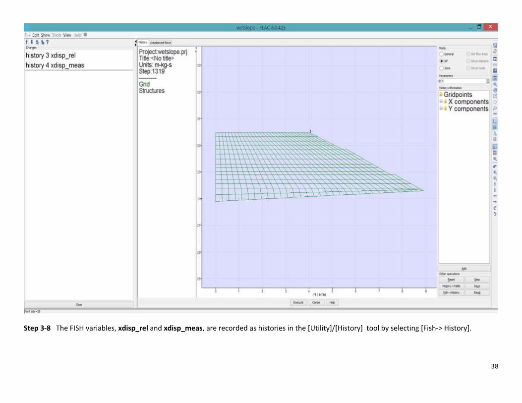
Step 3-8 The FISH variables, xdisp_rel and xdisp_meas, are recorded as histories in the [Utility]/[History] tool by selecting [Fish-> History].

39

Step 3-9 The model is run for 60,000 steps using the [Run]/[Cycle] tool.

40

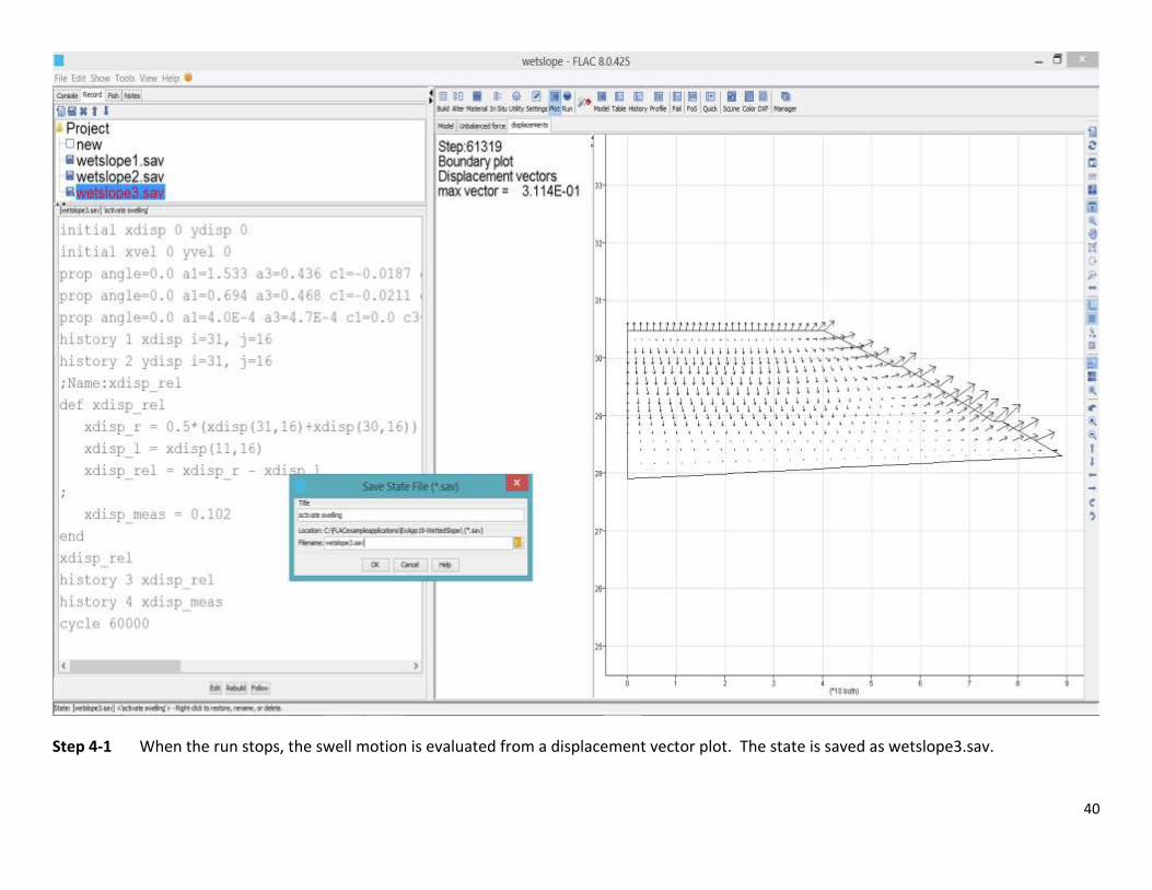
Step 4-1 When the run stops, the swell motion is evaluated from a displacement vector plot. The state is saved as wetslope3.sav.

41

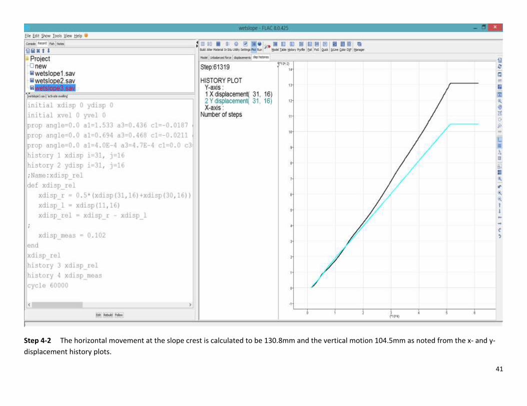
Step 4-2 The horizontal movement at the slope crest is calculated to be 130.8mm and the vertical motion 104.5mm as noted from the x- and y-

displacement history plots.

42

Step 4-3 The relative extension (swelling motion) along the slope crest is calculated to be 108mm, and is compared to the measured value of

102mm in the history plot above.