Embed Size (px)
Citation preview

• , '1.' , ,
~; . '-
.... ;- .. SVERIGES LANTBRUKSUNIVERSITET
-: :--.: -:.:.:-:-:-:-:.:-:-:-:-'-:-:-:.:- ..... .
.. . . .. . .... ..
......... ••••••••••••• ••••••• • •• •• •••• • ••••••••• (V~r •• ~ .• j)· ••••••••• • ••• • ••••••••••••• ) •••••••••
irll~ilettl~~! · I I Input files IISwitches IIParameter~ IOutputs 11 Execute I I
Technical
Model apeclft
Henrik Eckersten Per-Erik Jansson Holger Johnsson
"
Institutionen for markvetenskap Avdelningen for lantbrukets hydroteknik
Avdelningsmeddelande 96:1 Communications
Swedish University of Agricultural Sciences Department of Soil Sciences Division of Agricultural Hydrotechnics
Uppsala 1996 ISSN 0282-6569
ISRN SLU-HY-AVDM· -9611- -SE

Denna serie meddelanden utges av Avdelningen for lantbrukets hydroteknik, Sveriges Lantbruksuniversitet, Uppsala. Serien innehaller sadana forsknings- och forsoksredogorelser samt andra uppsatser som bedoms vara av i forsta hand internt intresse. Uppsatser lampade for en mer all man spridning publiceras bl a i avdelningens rapportserie. Tidigare nummer i meddelandeserien kan i man av tillgang levereras fran avdelningen.
Distribution:
Sveriges Lantbruksuniversitet Institutionen for markvetenskap Avdelningen for lantbrukets hydroteknik Box 7014 75007 UPPSALA
Tel. 018-67 11 85,6711 86
This series of Communications is produced by the Division of Agricultural Hydrotechnics, Swedish University of Agricultural Sciences, Uppsala. The series consists of reports on research and field trials and of other articles considered to be of interest mainly within the department. Articles of more general interest are published in, for example, the department's Report series. Earlier issues in the Communications series can be obtained from the Division of Agricultural Hydrotechnics (subject to availability).
Swedish University of Agricultural Sciences Department of Soil Sciences Division of Agricultural Hydrotechnics P.O. Box 7014 S-750 07 UPPSALA, SWEDEN
Tel. +46-(18) 67 11 85, +46-(18) 67 11 86

11', . ,',.
SVERIGES lANTBRUKSUNiVEIRSrrET'
Modol
Henrik Ecken:;tell1 Per~Erik Jall1ssoll1 Holger Johnssoll1
", ;'" ~.' ., ','
institutionen for markvetenskap Alfdelningen fOr lantbrukets hydmteknik
Alfdelningsmeddeiande 96:'1 Communications
Swedish University of Agricultural Sciences DepcU'tment of Soil Sciences Division of J\gricultural. Hvdrotechnics
IJppsala 1996 !SSN 0282-G!iGB
ISHN :'~!~IJ·'HY··/\, \lDlv)·, ··DGn· "SE


Table of Contents
1 Background ................................................................................................. 5 1.1 Model description ................................................................................ 5 1.2 Model application ................................................................................ 6 1.3 Flow schemes ....................................................................................... 8
2 Getting started ........................................................................................... 11 2.1 Installation ......................................................................................... 11 2.2 Files ..................................................................................................... 11 2.3 Running the model .... .......................... .............. ............ ..... ................ 12 2.4 Evaluating your simulation ............................................................... 1.2
3 Program structure ..... ..................... ........................... ........... ...................... 12
4 Files ............................................................................................................. 1.3 4.1 Input ..... ..... ...... .................. .......................... ..................... ........ ........... 13 4.2 Output.................................................................. ................................ 16
f) SWlrrCI-IES.".,"«, ... , ..... ,., ..... ,." . .,. <.,." •• ,., no., .. , .. ,', ........ " < •••••• , •••• ,............... 17 5.1 Technical............................................................................................. 17 5.2 Model specific ..................................................................................... 19 5.3 Special ................................................................................................. 22
6 PARAMETERS ........................................................................................... 27 6.1 External inputs (M) ............................................................................ 27 6.2 Manure application (M) ..................................................................... 29 6.3 Soil and Plant management (M) ........................................................ 30 6.4 Soil Profile and Site Description (S) .................................................. 32 6.5 Mineralisation and immobilisation (M) ............................................ 33 6.6 Soil abiotic response (S) ..................................................................... 35 6.7 Denitrification (S) ............................................................................... 37 6.8 Stream water (S) ................................................................................ 38 6.9 N root uptake (S) ................................................................................ 39 6.10 Leaf' assimilation (£0) ........................................................................ 41 6.11 Biomass allocation (£0) ...................................................................... 42 6.12 N allocation (P) ................................................................................. 45 6.13 Respiration & Litter (P) ................................................................... 47 6.14 Growstage (P) ................................................................................... 49 6.15 Plotting on line ........................ ........... ................... ...... ................ ..... 50 6.16 Special ............................................................................................... 51
7 OUTPUTS ................................................................................................... 61 7.1 States .................................................................................................. 61 7.2 Flows ........................................................................ ........................... 63 '7.3 Auxiliaries .......................................................................................... 69 '7.4 Drivings .............................................................................................. 74
8 Run options ................................................................................................. 76 8.1 Run no.: ............................................................................................... '76 8.2 Start date: ........................................................................................... '75 8.3 End date: ............................................................................................. '7t') 8.4 Output interval: .................................................................................. '75 8.5 No of'iterations: .................................................................................. '75 8.6 Run id: ................................................................................................. 75 8.7 Comment: ............................................................................................ 76

9 Execute.......................................... .............................................................. 76 9.1 Exit ...................................................................................................... 76 9.2 Run...................................................................................................... '76 9.3 Write parameter file ........................................................................... '76
10 Warnings and Errors ................................................................................ '76
11 Commands ................................................................................................ 76
12 Additional information ............................................................................. '7'7 12.1 Help ................................................................. , ...... ""." .. " ... ""."".". 77 12.2 Acknowledgement "'"'''' ........................................ ........................... 77 12.3 References................ ........ ...................................... ....................... .... '78 12.4 News ......................... ............................................... ......... ................. 80
Appendix 1: Variable number list ................................................................. 82
Appendix 2: SIMVB; Run SOILN under the Windows program ................. 84 How to run SO ILN .................................................. " ............................ ,... 84 Alternative use of SIMVB ..... ,................................................................... 85 Adaptation of application to SIMVB ........ , ....... , ............ , .......................... 8'7 Calibration of SOIL·SOILN ..... " .. , ......................... , ......... ,........................ 89 File description of SIMVB """"""" .......... , ........ , ..... ,................................. 91

1 Background Version 9,1; Uppsala 96-08-20
This manual is adapted to the SOILN model version 9,1 and is a development from Eckersten et al (1994), The model presentation is divided into one part which describes a basic and/or
original part of the model and one part including special/new options which you can get access to by setting the SPECIAL switch ON, By this switch thc model can be used as a tool for testing
alternative theories selected by the user, and to get access to special options useful for application of the model. This rcport can not be used as a reference for the validity of those theories, The
model is developed in close collaboration with several research scientists, The contributiou of different persons is given in Acknowledgement.
1,1 Model description The SOILN model simulates major C and N-flows iu agricultural and forest soils and plants.
The model has a daily time step and simulates flow and state variables on a field leveL Inpnt
variables are daily data on air temperature and solar radiation, management data and variables on soil heat and water conditions which arc simulated by an associated model named SOIL
(Jansson & Halldin, 1979). The model can conceptually be divided into two submodels: the soil submodel and the plant submodeL The soil part is described in detail by Johnsson et a!.
(1987) (Figs. la and b) and the plant model description is divided into onc part for the current year dynamics (Figs, 2a and b; Eckersten & Jansson, 1991) and one forthe perennial part (Figs,
3a and b; Eckerstcn, 1994). Note that the flow schemes in Figs 1-3 describe possible flows whereas the flows used depend on the model application, i.e, the choice of switches and
parameter values, Papers dealing with applications of the model are found in the reference list.
The soil is divided into layers, In each layer mineral N is represented by one pool for ammonium N and one for nitrate N, Ammoninm is immobile whereas nitrate is transported with the water
fluxes (a special option can make ammonium mobile), The ammonium pool is increased by nitrogen supplied from, manure application, mineralisation of organic material and by
atmospheric deposition, and it is decreased by immobilization to organic material, nitrification to the nitrate pool, and plant uptake, The nitrate pool is increased through nitrification of the
ammonium pool, fertilization, atmospheric deposition and by capillary rise of water from subsoiL It is decreased by leaching, denitrification and plant uptake. Water flows bringing
nitrate between layers, is the process finally responsible for N leaching. The daily output of N from the mineral pools might in case of low mineral N contents be bigher than available N plus
input, especially as concerns nitrate. To reduce this problem the following priority of access to N was used. First immobilisation to microbes, then nitrification and root uptake.
The organic matter is normally represented by two pools, however, there arc options to alter
the number of pools used and to choose if microbe dynamics should be simulated or not. The rate of decomposition of organic matter depends on soil water ancI temperature conditions.
Nitrogen dynamics of the organic matter is governed by those C flows and mineralisation or immobilisation depend on the C/N ratio of the decomposed material and availability of mineral
N.
Background 5

'rhe plant biomass and N dynamics are based on a strong relationship between carbon and nitrogen as used by Eckcrsten & Slapokas (1990), Eckersten (1991a), Eckersten (1994) for willow and (Eckcrstcn & Jansson, 1991) for wheat. The model concept has its origin in two basic model concepts; first that carbon input is strongly related to the energy input (de Wit 1965) and second, the nitrogen input is governing growth (Ingestad et a1. 1981).
The plant is divided into onc pool for biomass and one for nitrogen for each type of function simulated by the model. Leaves take up carbon from the atmosphere and roots take up nitrogen from the soil. Stem is used for storage. During grain development the grain pool is an additional storage organ supplied with assimilates from the stem. The maximum photosynthesis is related to the radiation intercepted by the canopy leaf area. The actual photosynthesis is then reduced by low air temperature, low leaf nitrogen concentrations and water deficit. N uptake is either limited by the sum of the demands by different plant tissues or the availability ofN in soil. The demand depends on the plant growth and wanted N concentration of tissues. The available soil N is a fi'action of the total mineral N in the root zone.
The partitioning of daily growth to root, leaf and stem is governed by two functions. The fraction partitioned to roots decreases as the total plant biomass increases or in case of nitrogen or waleI' shortage. The partitioning between leaves and stems depends on the leaf area development which is determined by the leaf area to shoot biomass ratio. During grain development biomass and nitrogen are allocated from different plant tissues to grain. Litter formation occurs continuously and tissues may redraw some of their biomass and N before they die. There arc different functions for governing the mortality of plant tissues. Dates of emergence, start and stop of grain filling and maturity are calculated as functions of temperature, daylength and a maximum harvest index.
In case of perennial plant there are additional pools for old plant biomass and a pool of easily available assimilates. The latter is added to the daily photosynthesis and re--allocated within the plant, and increases in proportion to the total biomass and temperature. The old tisslles have ;: smaller influence on growth than the younger ones. They affect the C and N dynamics by consuming assimilates for the maintenance respiration, by increasing available assimilates for growth and by increasing root depth. They also affect the input to the litter pools by the contribution of material with relatively low nitrogen concentration. The biomass of the young pools arc transf'crred to the old biomass pools at a certain age (normally one year) given by the user.
A more precise model description is gi ven in the section on Parameters where the most essential equations for different processes are found. The pmameters are given with their names whereas other variables arc given by normal mathematic symbols, the explanation of which is founc! within the section on Outputs.
102 Model application To enable a robnst application procedure of the model, certain developments have been made. A special program SIMVB (sce Appendix 2) allows the user a good overview when checking that all variables simulated by the model are reasonable. It also allows a handy way ofcomparison between simulations and measurements. In addition a special option is introduced (see BOUNDARY-switch) that enables simulated values to be replaced by measurements or values
G SOILN user's mannal

calculated by another model. This option is meant to be used if only parts of the SOlLN model is wanted to be studied, for instance when making step-wise calibration. It could also be used as an indicator of model performance (minimum correction corresponds to best performance).
The SOILN model includes a lot of parameters and there is no unique way of how to set those for a certain application. However, by following four calibration rules the number of possible solutions will strongly be reduced, depending on how many measurements there are available for the test of model outputs.
- Before start of calibration: Set input data according to independent data (measurements, literature etc) as far as possible and as correct as possible. Four calibration rules: - Change as few parameters as possible - Change only to parameter values that arc reasonable - Make documentation: Which fit was improved by a certain change? - Check that all variables simulated by the model are reasonable
Concerning the second rule (change only to reasonable parameter values) you should keep iu mind that sometimes the interesting output of the model application is that ruodcl could fit measurements only if unreasonable parameter changes were made. In this case it reflects non validity of the model concept, if other input data are correct. Concerning the third rule (documentation) also document the interaction betweeu parameter settings.
Normally, the model should be calibrated step-wise. In Appendix 2 an example of a procedure of how to calibrate the SOILN model is shown.
Background '7

1.3 Flow schemes
SOIL Carbon
Plant _ J I Incalltc I~~_~ docal0ac
AccnESPC
Manum
LlTABOVEC - de~~ft';-- ~ -~-~~- - --~------ - - Soil surface ...........................
L,. r- ~~'':-==-cl,,: !-r:rl:::,",'j';;; '2,: AGCRESPC
Plant aleafn3n awloafn3n
SOIL Nitrogen
Manure
. _._-_.- -_ .. __ ._-_ ... _-- .. -----_ .. _-----_.------
, uleallt
! U;~~OVE I
i I [decaleall
dearof ---decant
-r dccallt ne~nl
""'ll1II nlroff
SoH surfaco
Soil layer below
pipel
Soil layer below
Doposition Fortilizer ACCDENI
(~/)
~~ IIIGrtn03
':~-::""-':-=-' nflow(i)
nflow(i+1)
doni
Isurrno3
dIO$S
stream! I-,-~,----------" "' __ "" ______ ' __ " __ ~_~ ________ ~~"')
ACCDLOSS
Figure la and b, A schematic description of carbon and nitrogen flows and states of the soil part of the SOILN model. Symbols are explained in the section of Output variables, Microbial biomass and extra litter pool are not included in the scheme,
8 SOILN user's manual

Atmosphere New biomass
'-~-I~--J PI·IOS
arootliw
New nitrogen
Atmosphere .- -,- '----- -_.----------_/
depoleaf
ACCHARV &
ACCRESPC '---~-,~ ----_./
chalv
rosplw
halvlw
respgw
harvgw ____ r_E!~!~~_~
-11alvs'w'"
INCALlTC
NEWCL
.............. """ resprvv
nl1arv
1,"U"::0"::""',,3"" ~==.= ... ' ",,:r'L~IE;'A;'F;'N:' ·······--1 j' .................... . ................ _ .. " ... '._e_".I.I.ir_' _._. __ ~ __ . ________ ~ harvln asoiHn
harvgn
!;mvs" ... il'>-'
I asoilsn
INCALlT
asoilrn NEWNL
arooilin
Figures 2a and h. A schematic description of the biomass and nitrogen flows and states of the PLANT-submodel of SOILN model. The part concerning the current year growth. Symbols are explained in the section of Output variables.
Background f)

Old biornass
XAVAIW
aleafaw awleafaw
I aleafww ....................................................... .., awleafliw
LEAFW WLEAFW
asternaw awstomaw
STEMW
arootaw awrootaw ................................•......•.....•.... [,' ..... . awrooWw
INCAUTC
F100TV\f 1i>'Jw~IWI~OOTVV NEweL
ACCHARVC &.
ACCRESPC
resplw
respsw
arootww ............................................................................................................. ~
TOTUPT
X/"Vf\IN
aleafan
I·············· LEJ.\FN
asterna.n
STE:MN
Id n
awloafan
arootan awrootan
I,{OOTN
arootwn
resprw
Atrn_ospherc
depowleaf
awleafn3n
awleaflin
awsternan ................... awslto
..•......................... 1 awrootlin
Figures 3a and h. A schematic description of the hiomass and nitrogen flows and states of the PLANT-suhmodel of SOILN model. The part concerning perennial growth. Symhols are explained in the section of Output variables.
10 SOILN user's manual

2 Getting started
2;,] InstaHation The model is normally distributed together with the SOIL model on a special floppy diskette for IBM/PC. Two different installation diskettes can be used depending on whether you are a previous user of the PGraph program or not.
Type the command: @NSTALLA: C: X~,~ _____ -~
This means that you have inserted the diskette into a floppy disk drive named A: and you waut to install the model on your hard disk C: iu the directory named XXx, Normally XXX is substituted by snV! or SIMVB, If you already have a directory with that name you should choose another name at the installation,
2.2 Files The installation procedure will create one main directory (C:\SIMVB\) below which the program files arc stored in different subdirectories, The excitable files arc placed in the subdircctory named EXE and sample files in the subdirectory named DEMO,
Table 1: Description of files in the different directories,
Files
Directory: C:\SIMVB\EXE SOILNEXE Execute file, SOILN model SOILNDEF Definition file, SOILN model SOILNJILP Help file, SOILN model PREPJlXE Execute file, PREP program PG,l~XE Execute file, Pgraph program PGJILP Help file, Pgraph program PLOTPF,EXE Execute file, PLOTPF program PLOTPFJ-ILP Help file, PLOTP!" program
Directory: C:\SIMVB\DEMO\N DEMO,BAT Demo file for running the SOlLN model and using the PG program
AIN_ONE.P AR
AIN_CLIM,BIN AIN_SOWDAT SOILNTRA SOlLNXXX,BIN SOlLNXXX,SUM
Getting started
for visualizing some results on the screen. Initial conditions for running the SOILN model Parameter file for simulating nitrogen dynamics of an arable land with an agricultural crop during a growing season.
PG-file with climatic driving variables for running the SOILN modeL File with soil hydraulic properties, Translation files for variable names, SOILN Files with output variables from the simulation examples,
11
2.3 Running the model Before running the model you must make sure that the model and utility programs arc correctly installed on your computer. There must be a path to files store in directory C:\SIMVB\EXE (most conveniently in the AUTOEXEC.BAT file).
The DEMO.BAT file will be a good test of the installation and it will also show a number of results without any other efforts than running the DEMO.BAT file.
For running the program interactively use commands as specified in the section on Commands.
I PREP SOIL~ AlN_ONE
Is an example of how you can make your own simulation based on information in the AIN_ONE.PAR file.
2.4 Evaluating your simulation A successful simulation will result iu two different output files numbered as nnn :
SOILNnnn.SUM Contains a summary of simulation results in ASCn.
SOILNnnn.BlN A binary file comprising output variables from the simulation. You start the Pgraph program by typing:
PG SOILNnnn
For details on how to use Pgraph sce the Pgraph manual or use the help utility in the program (Fl key).
Another file created by the PREP program the first time you run the model in a certain directory IS:
SOlLN.STA which inclndes information about your run number. 'rhe numbering of a run within this file can be modified by the PREP program (see section 8 Run options)
3 Program structure The preparation of the model prior to a run follows an interactive dialogue where the user has the possibility to design the l'Un according to the present purpose.
The different menus can be reached in any order after moving the cursor to the subject using arrow keys and pressing "return" at the chosen subject. "Return" takes the cursor down in the menus and "Esc" moves the cursor up onc level. Normally, a user will start with the subjects to the left in the main menu and move to the right. It is a good rule to modify the settings of switches and input files before moving to the other menus, since the content of the lower mellUS is influenced by the setting of those above.
12 SOILN usees manual

4 Files
4.1 Input
Driving variable file FILE( 1) XXXXXX.BIN: A driving variable file is always a PG-me. The variables in the PG-file can be organized in different ways depending on how different parameters are specified. The driving variables for the SOILN model is generated by the SOIL model. The variables are identified by SOILN according to the names given below (sce Driving variables to get the description). They can also be identified with the model description given by the SOIL model. Layers must be given in order, from the top to the bottom. In the output file SOILNxxx.SUM you can check that your driving variables were correctly identified.
Tablc 2: Variables in cll'ivingvariable file (FILE(l)) to SOILN.
Name in the SOIL model
WFLOW 1Nl' INl'BYPASS Dl'LOW SURR TEMP THETA ETR PERC TA RIS MEACONC
Number of variables '--
[N-lI [I] [1 ] [N] [1 ] [N] [N] III [1] [ 1] [ II [ I ]
No (mm/day) No (mm/day)
Yes (mm/day) Yes (mm/day) No (mm/day) No Cc) No (vol %) No (-)
Y cs (mm/day) No Cc) No (Jm2/day)
Yes (mg/l) '-'-~~--"'----"--'--'~--'---.~,---~~---.
N is the number of layers in your simulation and this number must correspond to the value of the NUMLA Y parameter (Sce soil profile).
Parameter file FILE(2) XXXXXX.PAR: The parameter file is an ordinary DOS··file with ASCII- characters. All parameters with actnal numerical values should be included in the file. Parameters missing in the file receives the default value found in SOILN.DEF. New parameter files may be created prior the execution of the model Llsing the WRITE command (sce EXECUTION WRITE). Several parameter files conld be used. The information from the last incorporated file gets the highest priority, it "overwrites information from earlier parameter files and the SOILN.DEl' file.
Translation file FILE(3) SOILN.TRA: A translation file (ASCII) has to exist in order that the variables in the output PG-file should get their correct identifications. Only when the OUTl'ORN switch is ON, this file is not necessary.
Files 13

Initial states file FILE(4) XXXXXX.lNI: An ASCII file containing the initial values of all state variables that should start !i'om a value> O. The state variables denoted ACC. .. should normally be zero. Note that GROWINI-switch regulates if plant states should be read from this file.
Rules to write the file: I. The most simple and safe way is to write only one variable name at each row followed by a space and the value, for instance: LITABOVE 1.2 2. Up to 3 variables could be put on each row with the following format: variable 1-3 should be in columns 2 to 27, 29 to 54 and 56 to 81, respectively. 3. Layers is denoted within brackets, for instance: N03(3) 1.35 4. If different layers have the same value you could write for instance: N03(l-3) 1.35 5. The name of the state variable file must be defined in the xxx. PAR-file or be given in PREP under Input files.
If INISTATE-switch = 0: All initial states are zero.
Output file FILE(6) SOILNnnn.BIN: Only used if ADDSIM-switch "CO 1. The results of the current simulation are added to this file which contains output data from a previous simulation.
Validation file FILE(7) XXXXXX.BIN: A file with variables (measured) that should be compared with simulated variables. The result of the comparison will be found in the SOILNnnn.SUM file. The first variable in the validation file will be compared with the first variable in the output PG· file, the second with the second and so on. If V ALIDPG-switch ,= 0: Not used.
Soil physical properties FILE(S) XXXXXX.DAT: An ASCII file containing soil physical properties ofthe soil profile which arc used for the soil water and heat simulation with the SOIL model. The file is created by the PLOTPF program and must exist on the working directory. Only the porosity (PORO) and the water content at wilting point (WILT) are used in the nitrogen simulation. A complete description of the file is found in the SOIL manual (Jansson, 199Ib).
In the SOIL model, the thickness given for each layer in the SOlLP.DAT file can 1)(0 adjusted in the simulation (Parameters in the SOIL model: UDEP and LDEP, in easc UTI-lICK = 0, otherwise see UTHICK). Check your actual layer thickness used in the sum file of your SOIL simulation. If necessary adjust the layer thickuess in the SOILP.DAT file llsed for the SOlLN simulation. The result of these adjustments can be seen in the SOILNnnn.SOM file.
External inputs - driving variable file FILE(9) XXXXXX.BlN: Depending on the value of the switch DRIVEXT different parameters concerning fertiliser application are expected to he find in this file (at time 12:00). Date of application is taken from the date record in the file. If the first variable (FERN) is missing for a date, no other variables are reac\. If it is -99 then the other variables are reac!. If a variable value is -99 then it is treated as missing in the calculations. All values are reset to zero for intermediate time points. Only used if DRIVEXT-switch>O.
lA SOILN user's In<lnual

Table 3: Variables in FILE(9) for different values on the DRIVEXT-switch.
DRIVEXT-switch Variable (#) Parameter name in Unit model
I 1 FERN gNm,2
2 2 MANNH gNm'2
2 3 MANLN gN m"
2 4 CNBED (-)
2 5 MANFN gN m'
2 6 CNFEC (-)
2 ') MAN DEPTH (m)
3 8 DEPWC (mgN 1'1) --~~-.
3 9 DEPDRY m'2day'l)
Crop - driving variable file FILE(lO) XXXXXX.BIN: Parameters related to plant N uptake. Same roles for reading values as for FILE(9) except that values are not reset for intermediate time points, The values afe kept constant until a new value is read. Only used if the GROWTH-switch",O, BOUNDARY -switch",O and DRIVCROP·,switch>O.
'fable 4: Variables in FILE(lO) for different values on the DRIVCROP-switch.
DRIVCROP-switch
1
2
Variable (#)
1
2
Boundary - driving variable file
Parameter name in model
ROOTDEP
UPA,UPB ...
Unit
(m)
(gN m'2day')
FILE(lO) XXXXXX.BIN: Measured values of states, flows and auxiliaries to which the model should be fixed during simulation. Maximum 20 variables with their errors could be given. Variable that should be fixed to the value in the file is defined by parameter BOUNVNUM(nn). The parameter defines the number in X, T or G array of the model (see Appendix 2). Total number of variables in the files (including the error variables) is given by parameter BOUNFTOT. If the BOUNDARY -switch",3 the el'1'or variables should he omitted. The roles for reading values are the same as for FILE(lO) in the previous section. Only used if BOUNDARY-switc!l>O.
Table 5: Variables in FILE(lO) for different values on the BOUNDARY-switch.
BOUNDARY-switch
I
1
Files
Variable (#)
I
2
3
4
Value
Mean value varl
Relative error varl
Mean value var2
Relative error var2
Unit
(differ)
(-)
(differ)
(-)
15
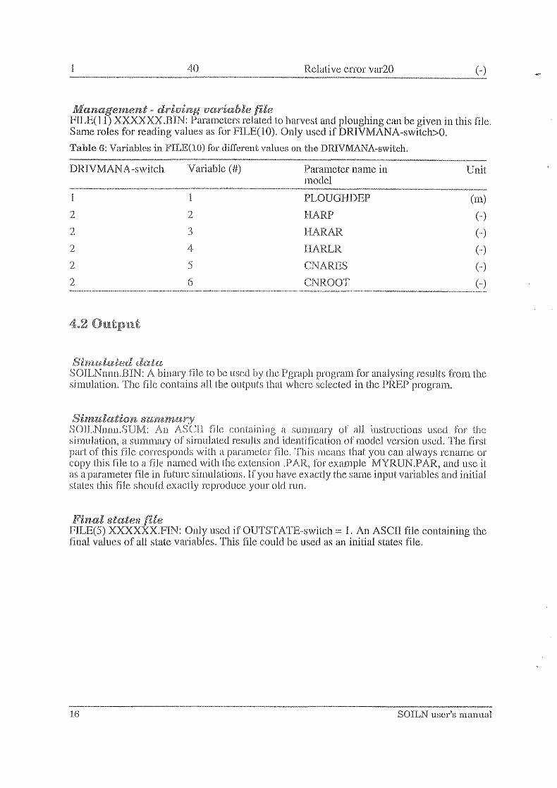
40 Relative error var20
Management" driviff&g variable file FILE(11) XXXXXX.BIN: Parameters related to harvest and ploughing can he given in this file. Same roles for reading values as for F1LE(lO). Only used if DRIVMANA-switch>O.
Table 6: Variables in FILE(lO) for different values ou the DRIVMANA-switch.
DRIVMANA-switch Variable (-it) Parameter name in Unit model
.-.~-----~~~,-~~~-----,
I PLOUGHDEP (m)
2 2 HARP (-)
2 3 HARAR (-)
2 4 HARLR (-)
2 5 CNARES c-)
2 6 CNROO'T' (-)
4.2 Output
Simulated data SOILNnnn.BIN: A binary file 10 be used by the Pgraph program for analysing results from the simulation. The file contains all the outputs that where selected in the PREP program.
Simulation SWnnrUJiFJ' SOTLNnnll.SUM: An ASCII file containing a ,;ummary of all in,;tructiol1s used for tbe simulation, a summary of simulated results and identification of model version used. The first part of this file corresponds with a parameter file;. This means that you can always rename or copy this file to a file named with the extension .PAR, for example MYRUN.PAR, and use it as a parameter file in future simulations. If you have exactly the same input variables and initial states this file should exactly reproduce your old run.
Final states file FILE(5) XXXXXX.FIN: Only used if OUTSTATE-switch '" I. An ASCII file containing the final values of all state variables. This file could be used as an initial states file.
SOILN user's manual

5 SWITCHES The purpose of switches is to choose the subroutines valid for you application. Switches can be OFF, ON or have a numerical value. You change value of a switch by putting the cursor at the switch and press the return key. Switches may be hidden if some other switches make them irrelevant. After you have modified a switch the modification is activated by escaping [ESC] the menu. By entering the menu again, immediately after the escape, you see whether some more switches have become visible because of the previous change. Note tbat also new parameter settings might appear. (Group names given within brackets (S, P, M or 0) refer to Soil, Plant, Management and Others)
5),1 Technical
ADDSIM
OFF The simulation results will be stored in a separate result filc with a uumc Def~~~ ____ ~a~c~c~ol~'d~i~ng~~to~tl~le~r~u~n~n~u~m~b~el~·._~~~~02) ____ ~ .• ______ ._. ___ • __ . _______ .. ~ ON 'fhe simulation results are automatically added to the result file of a previous
simulation, l'lm for an earlier time period. Note that the selected output variables must be exactly the same for the current and the previous simulation. The name of the former result file is given by the user as the "output file" name (see FILE(6)). By default the start elate of the present simulation is put identical to the terminate date of the previous simulation. The final valucs of statc variables from the previous simulatiou must be selected as the initial values of state variables for the present run (see INSTATE and OUTSTATE switches). Note that the OUTSTATE switch must be ON for any simulation to which results of a later simulation will be added. No new result file ".BIN" will be created, but a separate summary file ".SUM" will be created just like for an ordinary simulatioll.
~-----~~--.-,,--~-.~---
AVERAGED
OFF
ON Default
All requested driving (=D) variables will be the current values at the end of each output interval. See also A VERAGEX~switch. (Group 0)
"---'----~----I
All requested driving (=D) variables will be mean values representing the whole output interval (see section on Output interval). The output interval is represented with the date in the middle of each period.
AVERAGEG
OFF All requested auxiliary (=G) variables will be the current simulated values at the end of each output interval. See also A VERAGEX~switch. (Group 0)
-ON All requested auxiliary (=G) variables will be mean values representing the J)(!/rlUit whole output interval (see section on Output interval). The output interval is
represented with the date in the middle of each period. -
SWITCHES 17

AVERAGET
OFF All requested flow (=T) variables will be the current simulated values at the end of each output interval. See also AVERAGEX-switch. (Group 0)
ON All requested flow (=T) variables will be mean values representing the whole Default output interval (see section on Output interval). The output interval is
represented with the date in the middle of each period.
AVERAGEX
OFF All requested state (=X) variables will be the Clll'rent simulated values at the end of each output interval. If all switches A VERAGE._ are OFF the date giveu in the PG-output file is also the date of the end of the interval. Otherwise the date is the middle of each output intervals. (Group 0)
ON D~fault
All requested state (=X) variables will be mean values representing the whole output interval (see section on Output interval). The output interval is represented with the date in the middle of each period.
----------~~----------------------------~-------------------~
CHAPAR
OFF De/tlUit
1-- . ON
DR.lVff:'o,
Parameter values are constants for the whole simulation period. (Group M)
Parameter values may be changed at different dates during the simulation period. If you edit the parameter file then all parameter values given after a definition of a new time point will be activated when the simulation has rcach that point in time. A maximnm of 20 dates can be specified.
~) No function (Group M)
J Driving variables will be read from a Pgraph file. The name of the file is D~fault specified by the user. See Driving Variable File for details. ~----~----~----------~-------------. --------~
INSTATE
OFF All initial state values are zero (Group S)
ON initial values of state variables will be read from a file. The name of the file is Default specified by the user, the format should be exactly the same as in the file for
final values of state variables, created hy the model when the OUTST ATE switch is ON.
LlSALLV
OFF only the subset of output variables selected by the user will be found in the summary file. (Group S)
ON all output variables will be found in the summary file after the simulation. Default
18 SOILN uscr~s manual

OUTFORN
OFF D~t(lUlt
ON
OUTSTATE
OFF Default
ON
the variables will be named according to the information stored in the file SOILN.TRA. (Group 0)
all variables in the output Pgraph-file will be named according to their FORTRAN names.
no action. (Group 0)
final values of state variables will be written on a file at the end of a simulation. The name of the file is specified by the user and the format is the same as used in the file for initial state variables (see the INSTATE switch). _.. .-~~ .. ~ .. ~~-.. -~-~--~.~-~
VALIDPG
No validation. (Group 0)
Validation variables will be read fronl a Pgraph file. The name of the file is specified by the user. The values in the validation file will be compared with variables from the ontput file.
502 Model specific Switches denoted GROW .... are only nsed if GROWTH··switch = 1.
DENDIST ... ~ ..... 0 Denitrification rate distrihution from parameter values, separate fractions arc Defilult given for each soil layer (sce DFRAC) (Group S).
I A linear decrease of denitrification rate from soil surface to the depth specified by the parameter DENDEPTH.
2 A constant denitrification rate from soil surface to the depth specified by the parameter DENDEPTH.
3 An exponential decrease of denitrification rate from soil surface to the depth specified by the parameter DENDEPTH.
DRIVCROP --0 Plant development is simulated (i.e. the GROWTH-switch> 0) or specified Default by parameter values in parameter file. (Group S)
I The root depth is read from a driving variable file (FILE( 10)). Only used if BOUNDARY -switch=O.
2 As for 1 but also the potential N-uptakc rate is read from the same file.
SWITCHES 19

DRIVEX'1'
0 Parameter values for external input s of nitrogen to the model arc specified in DejllUit r--; parameter files. (Group M)
I N fertilization rate is taken from a - driving variable file (FILE(9)). -------~~~~-4
2 As for 1 but also parameters for app lication of manure are taken from the same file.
3 As for 2 but also parameters for wet and dry deposition are taken from the same file.
DRIVMANA
0 D~fault
1 -2
OFF De/lwit
ON
Parameters of management operations are taken from parameter file. (Group M)
Ploughing depth is read from a driving variable file (FILE(I 1)).
Also harvest and re··circulation of crop rcsiducs arc taken from the same file.
CUrfeut year old leaves are transferred (at the end oflhe year, normally) to old leaves according to leaf j~tll functions given by the user. Only used if GROWPREN·switch""l. (Group P)
All remaining leaves are falling to the ground at the cnd of the year. -~--~--~~--~,.~~-~,.~-~~~~-~~~,,-
GROWGRA1N
0 Def(wll
I
mWWINI
OFF
ON D~fclUlt
20
• No grain development. (Group P)
Grain development may occur (sec related parameters GRAINI, AGRAIN, AGRAINN). Only used if GROWPHEI\)-switch > Cl.
Plant initial values (annual biomass pools only) are calculated from parameter (TOTW(l)). N plant values are set assuming maximum N concentrations. (Group P)
Plant initial values for the first growing period are taken from initial file (FILE(4)). TOTW(l) is not used. For the second growing period TOTW(2) should be used.
SOILN user's manual
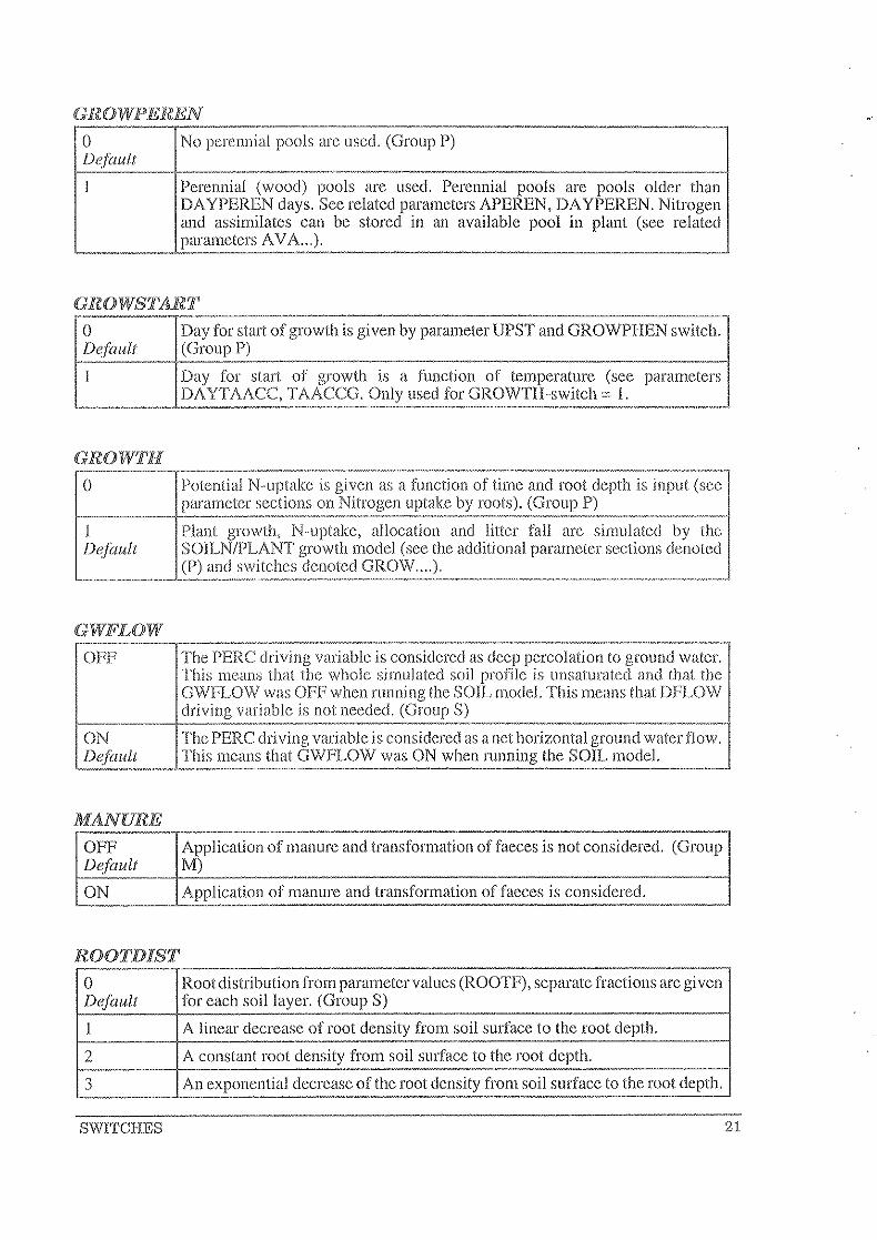
GROWPERE1V
o Default
No perennial pools arc used. (Group P)
Perennial (wood) pools are used. Perennial pools are pools older than DA YPEREN days. See related parameters APEREN, DA YPEREN. Nitrogen and assimilates can be stored in an available pool III plant (see related parameters A V A ... ).
GlWWSTART r-" o Day for start of growth is given by parameter UPST and GROWPHEN switch. Default (Group P) r-~~'---+~--~----~- .. -.-----.------------------------.------.-
Day for start of growth is a function of temperature (see parameters DA YTAACC, TAACCG. Only used for GROWTH-switch = 1.
,--------~-------
GROWTH
o Potential N-uptake is given as a function of time and root depth is input (sce parameter sections on Nitrogen uptake by roots). (Group P) - ... --~-.-+-----.~----.---~-~~-~-~--"------'~.--------I
I De/cwlt
Plant growth, N-uptakc, allocation and litter faJ! are simulated by the SOILN/PLANT growth model (see the additional parameter sections dbuv,cou
(P) and switches denoted GROW .... ). _. ____ ._ .. __ .L~.:~ .... ___ ._ ... __ . __ .... _____ . ___ . __ .... _ .. c_ ... _ .... ___ ...... _ ... _."' ........ """" ......... " ... ...J
The PERC driving variahle is considered as deep percolation to ground water. This means that the whole s.inmlated soil profile is unsaturated and that the GWFLOW was OFF when running the SOIL model. This means that DFLOW driving variable is not needed. (Group S)
.~----~~~~~--~----~-
ON The PERC driving variable is considered as a net horizontal ground water flow. Default This means that GWFLOW was ON when running the SOIL model.
,-,;:.......~~--"--
MANURE
OFF Application of mauure and transformation of faeces is not considered. (Group DefCLUlt M) ON Application of manure aud transformation of faeces is considered.
ROOTDIST --0 Root distribution from parameter values (ROOTF), separate fractions are given Default for each soil layer. (Group S)
I A linear decrease of root density from soil surface to the root depth.
2 A constant root density from soil surface to the root depth.
3 An exponential decrease of the root density from soil surface to the root depth.
SWITCHES 21

SPECIAL
OFF No special functions arc active. (Group M) Defilult
ON Special functions are available. Gives access to the switches and parameters in the groups named SPECIAL Note, that now the control of the special functions are made with these switches and parameters.
5,3 Special These switches activates special options of the model and are only available if the SPECIAL-switch is ON (= 1).
BOUNDAIlY
0 D~f(lult -~-.
I
_. 2
3
4
o Default
2
22
No corrections of simulated values during simulation. (Group M)
---Values in a driving variable file (see FILE(lO») are used for correction, during simulation, of simulated states, nows or auxiliaries (sce parameter BOUNVNUM(nn) and Appendix I). For each time point given in the file, correction is made to the given value, in case the simulated value is outside the error limits. States are corrected prior each timestep, nows immediately prior integration and other variables immediately after being set in the model. Errors given in the file arc relative errors. Total number of variables in the file is set by parameter BOUNFTOT. Only used if DRIVCROp··switch=O.
The same as for 1 but errors given in the file arc absolute values.
The same as for I but no error variahles are given in the file. Relative error is given hy parameter BOUNRERR. -The same as for 3 but no external file is used (i.c. FILE( J 0). Instead the values to which variables should be corrected should be given 111 parameters BOUNVALU(l-20). The correction is made every timestep (day).
-~
No action. (Group M)
Fertilisation is calculated by the model as the difference between the potential uptake and the actual uptake of the previous day. To this amount could be added a fraction given by the parameter A VAILN. The amount simulated by the model (FERNSIM) is added as ammonium and IS incorporated 111
FERTNH4.
Fertilisation is calculated by the model as the difference between the wanted soil N mineral amount (given by parameter A V AILN) and the sum of the mineral pools, the deposition and fertilisation and a preliminary estimation of mineralisation from organic matter. The amount simulated (FERNSIM) is added as solid fertilisers and is incorporated in FERTN03.
SOILN user's manual

GROWAEQ
13250 D~fClUlt
A combined switch selecting which type of allocation equations that will be used. (Note should be >10000) The first figure is the way different root allocation sub functions (b,w, 10"" b,J should be combined. 1: b,. = max(b,w, b"" b,el 2: b, = b,w*b,,,*b,., and 3: b, = (b,w +b,.,,+b,·c)/3. The second figure is leaf-stem allocation (b;; parameter ALEAF). The third is the root allocation as function of total plant biomass (b,w; parameter AROOTW). The forth is root allocation as function of leaf nitrogen (b,.,,; parameter AROOTNI). The fifth is root allocation as function of trauspiratiou ratio (b,e; parameters AROOTE and AROOTETR). The figures can range from 0 to 5 and means that different equations are used to estimate the function. 0: function is not active (not allowed for b;), I: yoca, 2: y'=a+b*x, 3: y=a+b*ln(c*x), 4: y=a+b*exp(c*x), 5 y=other equation. Coefficients a, band c arc the indices 1, 2 and 3 of the parameter. Example: GROW AEQ"d25 means b;=ALEAF( 1)+ALEAF(2)*ln(ALEAF(3)*WT,,);
b,w=AROOTW(1)+AROOTW(2)*W,; b,,,= special (scc AROOTNI). As regards x and other equations (5), see the parameter name concerned. NOTE! When changing GROW AEQ, the meaning of tbe parameters cbanges (ALEAF, AROOTW, AROOTNI). (Group P)
.~~--L_
Default
During grain development, reallocation of assimilates occur from leaf to grain (flows ALEAFGW and ALEAFGN), root to grain and stem to grain (flows AROOTGW and AROOTGN). (see parameters AGRAIN and AGRAINN). Flows AROOTSW and AROOTSN = () (Group P)
During grain development, reallocation of assimilates occur from leaf to stem, root to stem and stem to grain (see parameters AGRAIN, AGRAINI\I, ADRAWLW, ADRAWLN). __ --L ___ ~, _____ .
GlWWGEQ Determining the calculation of the growth response function (fro')' If GROWPHOS = 1 then fr is not included in the functions. (Group P)
() fro, = Min(fT, fN> fw)
1 fro, = 1'1' "' fN * fw Default
2 fro, = (fT + fN + fw)/3
SWITCHES 23

GROWPHEN
0
I Dej(lUlt
2
o D~f{lUlt
No phenologic functions arc active. Day of emergency is given by parameter UPST and day of harvest is given by parameter UPET. (Group P)
Start of grain development is an accumulated function of air temperature and day length. Otherwise as for GROWPHEN '" O.
Day of emergency is a function of accumulated temperature since sowing. Day of sowing is given by the UPST parameter. Day of start of grain filling is calcnlated as for GROWPHEN '" 1 except that accumulation of the index starts at day of emergency and not UPST. Day of end of grain filling is a function of accumulated temperature since start of grain filling. Day of harvest is a function of accumulated temperature since day for end of grain filling. The routine is taken from AFRCWHEAT model (Porter, 1984).
~-
Leaf assimilation is calculated using the radiation use efficiency concept. (Group P)
~---------------Leaf assimilation is calculated using a light response curve for photosynthesis taking account of growth respiration (France and Thornley, 1984) using the
1'~·ld~d~it~io~n~a~1~~~~~~P~P~M~iA~·~X~2~0~,I~)'10'R~j~\N~S~M~,~a~n(~J£P~G:~R~E~·S~P·~. __ ~ ___ ~ _______ j .~-----~------+ 2 The same as for (0) hut the nitrogen response for photosynthesis is a linear
function of total (annual) plant N concentration. This means that parameters NLEAFXG and NLEAFN arc used to represent the total N concentration at which photosynthesis is at maximum and minimum.
LlTTKCN
Cl i The specific decomposition rate of litter (UTK) and faeces (FECK) arc Defiwlt A. 11 of C/N ratio. (Group S)
1 The specific decomposition rale of litter (UTK) can be sct a linear function of the C/N ratio. IfMICROB-switch>O then MICK(l-3) is function of C/N ratio.
--.~~- --~-~-~-~-
2 As for 1 but for faeces (FECK).
3 I Both I and 2 above.
24 SOILN llscr~s manual
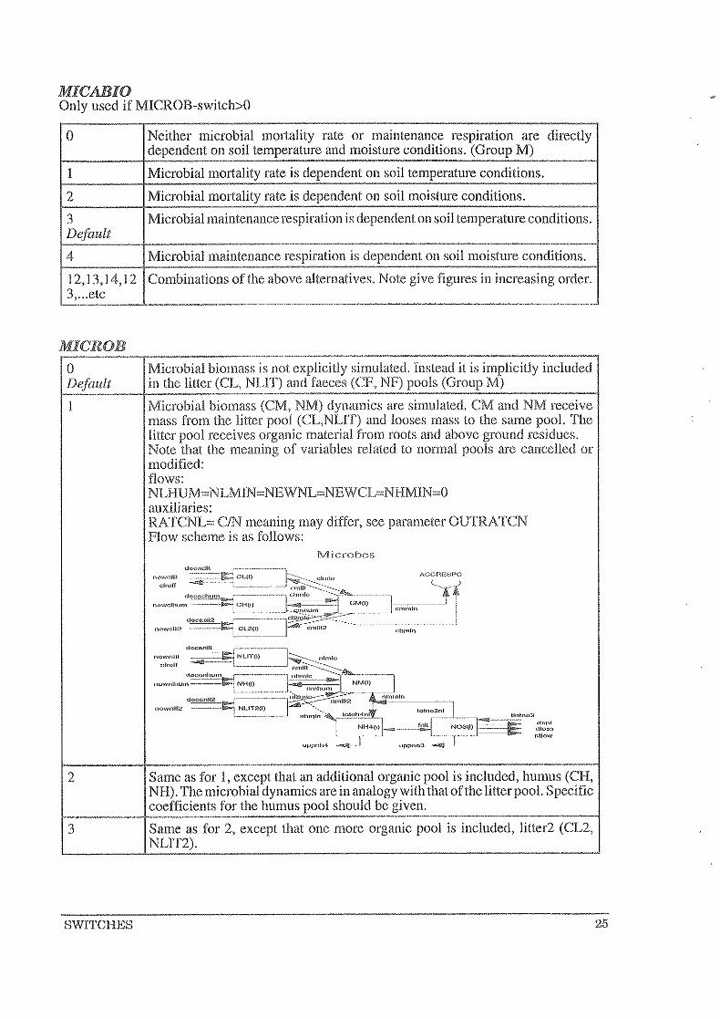
MICABIO Only used if MICROB-switch>O
0
1
2
3 Default
4
12,13,14,12 3, ... etc
I
Neither microbial mortality rate or maintenance respiration are directly dependent on soil temperature and moisture conditions. (Gronp M)
Microbial mortality rate is dependent on soil temperature conditions.
Microbial mortality rate is dependent on soil moisture conditions.
Microbial maintenance respiration is dependent on soil temperature conditions.
Microbial maintenance respiration is dependent on soil moisture conditions.
Combinations of the above alternatives. Note give figures in increasing order.
Microbial biomass is not explicitly simulated. Instead it is implicitly inclnded in the litter (CL, NUT) and faeces (CF, NF) pools (Group M)
Microbial biomass (CM, NM) dynamics are simulated. CM and NM receive mass from the litter pool (CL, NUT) and looses mass to the same pool. The litter pool receives organic material from roots and above ground residues. Note that the meaning of variables related to normal pools are cancelled or modified: flows: NLHUM=NLMIN=NEWNL=NEWCL=NHMIN=O auxiliaries: RATCNL= C/N meaning may differ, see parameter OUTRATCN Flow scheme is as follows:
Microbes
ACGFtESPC
( ) JA
2 Same as for 1, except that an additional organic pool is included, humus (CH, NB). The microbial dynamics are in analogy with that of the litter pool. Specific coefficients for the humus pool should bc given.
3 Same as for 2, except that one more organic pool is included, litter2 (CL2, NUT2).
SWITCHES 25

- . ---.-.-. - - ---4 Same as for 2, except that the humus pool is iucIuded in the way it is used in
the original model, i.e. mineralisation occurs directly from humus, proportional to the humus N and independent ofthe simulated microbial activity. In addition to the original model, respiration from humus (CH) is calculated. (The flows CHMIC=NHMIC=O, NHMIN>O, CHMIN>O)
91,92,93,94 Same as for 1-4, except that microbial gross consumption rate is proportional to substrate amount instead of microbial biomass.
-
NH4MOBIL
° Ammonium in soil profile is immobile. (Group M) D(~fault
I A fraction of ammonium is adsorhcd to solid particles and the soil water and is mobile betwecnlayers, in analogy with nitrate flow.
OPTWATER
10 Walerresponse functions for soil biological activity and plant growth are ,wtivp I Defau if (Group M)
I Soil NB4 mineralisation or immobilisation is not limited by soil water conditions.
2 Plant growth IS not limited by plant \vater condi tion s. Only for GROWTH-· switch = 1.
3 Optimum water conditions arc assumed for the allocatioll of assimilates ) root function. Only used for GROWTH-switch", I.
13,123,2 Combinations of the above alternatives. 3
TEMPREQ ---_._--- ._---------------_.- "-() The temperature response function for soil biological processes is calculated Default from the Q,o expression in the whole range. (Gronp S)
I The temperature response function is calculated from the Q,oexpression when the temperature is above TEMLIN. Below that a linear decrease is assumed towards ° °C where the response diminish.
2 The temperature response function is calculated from a quadratic response function (Ratkowsky fuuction). Note that the TEMBAS parameter change meaning.
3 The temperature response function IS calculated from a second order polynomial. _.- .. _---
4 Separate parameters l1lay be used for mineralisation, nitrification and denitrification.
14,24 Combinations of the above alternatives. ----
2G SOILN user)s ID.anual

6 P ARAlVIET:ERS Paramctcrs arc grouped in accordance to the processes they belongs to. The most important equations arc given in the top of each section. The basic ideas behind the equations arc given as concerns soil by Johnsson et al. (1987) and as concerns plant Eckersten & Slapokas (1990) and Eckersten & Jansson (1991).
All parameter values may be modified in the PREP-program by pressiug the return key when the cursor is located at a certaiu parameter. A new numerical value may then be specified and is loaded wben you go back to the top menu again [Esc].
Beneath the unit in the parameter description a value is sometimes givcn. This is a default value given by SOILN.DEF file. In the head of each parameter group is given (S), (P) or (M) denoting Soil, Plant and Management, respectively.
m
6.1 External inputs (M) ,m: $:_ - 0/
Dry and wet deposition to the soil surface is determined by a dry deposition rate (DEPDRY) and the water supply rate (the driving variables infiltration and surface run off) multiplied by the concentratioll of total nitrogen in precipitation (DEPWC). The ammonium N fraction (DEPFNH4) enters the ammonium pool of the uppermost soil layer whereas the nitrate is separated between surface runoff and infiltration. Commercial fertilizer N (FERN) is applied at a certain clay (FERDA Y). The fertiliser is dissolved at a constant rate (FERK) and a ccrtain fraction (FERNFNH4) cnters the ammonium pool whereas the rest enters the nitrate pool. Under conditions of a water source flow to the soil, this flow can also he a source of nitrogen (scc GWCONC). Dry deposition can also be directly taken up hy leaves (DEPDRY A).
NIl,,,.,.,NH4 '" DEPDRY*DEPFNH4D + DEPWC*(q,,,,H]Smc)*DEPFNH4W NIl,,,,',,'+Sm, = DEPDRY*( I-DEPFNH4D) + DEPWC*(q,,,r+qs,,,J*( I-DEPFNH4W)
N",,,_,, '" DEPDRYA*A,
NF",_,N'" ,= FERNFNI-14*FERK*NF,,, NF",.",,,,+,,,,,. ,= (1-FERNFNH4)*FERK*NF",
NI_,lnf:::: see N allocation N1w.,.-)!nf::: see N allocation
N 1nf->N03 ::::: X*qln!(qlnf+qSurr)
NS\lrr->Strclllll ::::::: x*qSur/(qlnC+qSun.) where: x:::: NDep--)!nf+surr + NFcrt-_.)!nf+Surr + Nl-->lnf + N1w->Jnf
DEPDRY Dry deposition of mineral N to soil nitrate and/or ammonium. A value of 0.001 correspond to 3.65 kg N/ha/year. Normal range for an open field in southern Sweden 0.0005 - 0.002 gN m'2 d". If DRIVEXT-switch '" 3: Then DEPDRY is read from FILE(9)
PARAMETERS
(gN m 2 cl") OJJOl
27

DEPDRYA Dry deposition of mineral N on canopy per unit of leaf area and which is taken up by leaves. Only used if GROWTH-switch = 1
DEPFNH4D Fraction of ammonium N in DEPDRY. The rest is nitrate N
DEPliWH4W Fraction of ammonium N in wct deposition given by DEPWC. The rest is nitrate N
DEPWC Concentration of mineral N in infiltration and surface runoff. During a year with 800 mm infiltration a value of 0.8 corresponds to a wet deposition of 6.4 kg N/ha/year. Normal range for southern Sweden 0.8 - 1.8 mg/l and for central Sweden 0.4·, 1.0. IfDRIVEXT,switch = 3: Then DEPWC is read from FILE(9)
FERDAY Fertilization date (commercia! fertilizer).
FERl( Specific dissolution rate of commercial fertilizer (not the ammonium N, if any). A value ofO.15 corresponds to half time 0[5 days and that 90% of the fertilizer is dissolved within 15 days. A higher valne results in faster dissolution. Dependent on fertilizer type and moisture conditions. Normal range 0.05 -0.5.
FERN N·,fertilization (commercial fertilizer) I gN m,2 = 10 kgN/ha. Normal range 0 - 30 gN m". IfDRIVEXT-switch >= 1: Then FERN is read from FILE(9)
FERNFNH4 Fraction of dissolved solid N fertiliser that is ammonium. The rest is nitrate N
GWCONC Concentration of nitrate in deeper groundwater. Input of N to profile from below is visible by DFLOW (driving variable) at the lower boundary being < O. The negative value is added to the flow DLOSS. Depends on the local conditions. Normal range 0.1 - 5.
(-) o
H o
(clay number) 140.
(lrl) 0.15
(-) o
(mgN rl) 0.3
28 SOILN user's manual

·m
Manure can be applied during three different periods according to day numbers assigned to MANST and MANET. The manure-N is split up between inorganic forms as ammonia (MANNH), organic forms as faeces-N (MANFN) and Iitter-N (MANLN). The organic forms of manure arc described by carbon-nitrogen ratios CNBED and CNFEC for litter and faeces respectively. Applied manure is mixed into the soil down to a depth given by the MANDEPTH parameter.
CNBED C-N ratio of bedding in manure (index= application period 1,2 or 3) Only used when the MANURE switch is ON ane! DRIVEXT < 2 Normal range from 20 to 80. Default value 30.
CNFEC C-N ratio of faeces iu manure (index= application period 1,2 or 3) Only used when the MANURE switch is ON and DRIVEXT < 2 Depend on type of animals. Normal range 10 - 30. Default value 20.
MANDEPTll Depth to which the applied manure is uniformly mixed into the soil (Index= application period 1,2 or 3). Only used when the MANURE switch is ON and DRIVEXT < 2 Maximum depth'" depth of layer 1 +2. Normal range O.S - 0.25 m. Default value O.lO m.
MANE'J.' Last date of manure application (index= application period I, 2 or 3) Only used when the MANURE switch is ON anci DRIVEXT < 2 lfMANET is given the same value as MANST the application of manure is made during one day.
MANFN Nitrogen in faeces in manure (index= application period 1,2 or 3). Only used when the MANURE switch is ON and DRIVEXT < 2 Normal range 0 - 30 gN m-2
•
MANLN Nitrogen in bedding in manure (index= application period 1,2 or 3). Only used when the MANURE switch is ON and DRIVEXT < 2 Normal range 0 - 5 gN m-2
•
PARAMETERS
(-) 30.
C·) 20.
(m) 0.1
(day !lumber) 100.
(gN nf')
29

lVlAlVNll Nitrogen in ammonium in manure (index= application period 1,2 or 3), Only used wheu the MANURE switch is ON and DRIVEXT < 2 Normal range ° -30 gN m-2
,
lVlAlVST First date of manure application (Index= application period 1,2 or 3) Only used when the MANURE switch is ON and DRIVEXT < 2
~t3 SOlH and Plant management (M) , rc'
(day number) 100,
71"
At start of growth or simulation a certain amount of plant biomass exists on the field crOTW(i); 1,3 depending on which cultivation of the year is conccrned),
Harvest of plant can take place at three different dates (UPET), At these dates a fraction of leaves (I-lARL) and a fraction of stems (HARS) are harvested, Another fraction remains alive: HARLL for leaves and HARLS for stems, The rest is included in the pool for above ground residuals (sce output variables INCA LIT and INCALlTC), Concerning the roots a fraction remain alive (HARLR) and the rest is included in the litter pools in the horizon in accordance to the root depth distribution (sce output variables NEWNL and NEWCL), At the day of ploughing (PLODA Y) all remaining living leaves and stems, and roots down to a depth given by PLOOGHDEP, all above ground residues are evenly included in the litter pools down to a depth of PLOUGHDEP, Tbe living roots below PLOUGHDEP arc incorporated in the corresponding litter pools, Note, it is not possible to barvest at the same day as plougbing is made,
If GROWTH-switch =, 0 then plant N is in focus, The plant is split into a harvested fraction (HARS), a fraction of plant residues above ground (HARLR) and a fraction of remaining living biornass··N (HART.) The residual (IHARS--HARLR-I-IARL) is considered as dead root N, The dead root N is included into the litter--N pool and split between different soil horizons according to the depth distribution of roots (see parameter ROOT), Tbe dead root C content is sct according to a carbon-nitrogen ratio of roots (CNROOT),
CNAlIlES C-N ratio of above ground residues Normal range 20-100, Default value represents a grain crop, If GROWrll-switch > 0: Not used, If DRIVMANA-switch = 2: Not used,
CN1W01' C-N ratio of roots Normal range 20-30, If GROWTH-switch> 0: Not used, If DRIVMANA-switch = 2: Not used,
I1IA1I?AR Above ground residue fraction of plant N at harvest (index", growth period 1,2 or 3) If GROWTH-switch> 0: Not used, If DRIVMANA-switch = 2: Not llsed,
Cl 50,
(-) 25,
( -) o
SOILN uscr)s manual

HARG The fraction of grains that is harvested. If GROWTH-switch ~ 0: Not used. If DRIVMANA·switch = 2: Not used.
HARL The fraction of leaves that is harvested. (index= growth period 1,2 or 3) If GROWTH-switch = 0: Not used. If DRIVMANA·switch =, 2: Not used.
HARLL Fraction of leaves alive after harvest. (index= growth period I ,2 or 3) If GROWTH-switch = 0: Not used
HARLR Fraction of roots alive after harvest (index= growth period!, 2 or 3) If GROWTH-switch = 0: The fractiou refers to plant N (PLANT) IfGROWTfl··switch = I: The fraction refers to root (ROOTN and ROOTW) IfDRIVMANAswitch = 2.: Not used.
HARLS Fraction of stems alive after harves!. (index= growth period I, 2. or 3) If GROWTH-switch = 0: Not used.
HARP Harvested fraction of plant N (index = growth period) .. ]) If GROWTH-switch> 0: Not used. If DRIVMANA·switch ,= 2.: Not used.
Tl'ARS Fraction of stems that is harvested. (index = growth period 1-3) If GROWTH-switch = 0: Not used. If DRIVMANA·switch = 2: Not used.
PLOUGHDAY Date of ploughing or soil cultivation. Note, mLlst differ from harvest day UPET.
PLOUGHDEP Depth of ploLlghing or soil cultivation Normal range 0.05 - 0.30 m.
P ARAMETgl{S
(-) O.
(-) O.
H o
( .. ) O.
H o
C) 0.5
(-) 0.5
(day number)
(m) 0.25
31

TOTW (W,(to)) Total plant biomass at start of growth. (index= growtb pcriod 1,2 or 3). Maximum N-concentrations are assumed at the start. GROWINI-switch=l implies TOTW(l) is not used.
UPET (U End of plant nptake period and harvest date (indcx= growth period I, 2, or 3)
(CROP): If the GROWTH-switch is 1,3, or 4: UPET(i)=367 implies the current growth period is not ended until the simulation is ended. UPET(i»367 implies that the growing period (i) is stopped at day UPET(i)-365. Should be: UPSTCi)<UPETCi)<UPST(i+ 1) If UPET is given a negative value then: tc=-UPET and the root biomass remains unchanged.
UPS'!' (to) Start of plant uptake period (index= growth period 1, 2 or 3) (CROP): If the GROWTH-·switch is t, :1 or 4: The parameter equals the earliest day for start of plant development. The temperature may delay the start of growth from this date. Should be UPST( 1 )<UPST(2)<UPST(3)<366. UPST(i)=O implies the period (i) is cancelled (OBS! This parameter is related to UPET (this parameter group) and 'I'OTW (Crop Biomass group)).
(day number) 240.
(day number) 120
'~~"~~~~~~~~_'~'~'~~'~'~ ______ ~~~~~~ __ -='~A@
6.4 SoH Profile and Site Description (13) ~ . m y
The soil profile is divided into a number of layers (NUM LA Y) with different thickness (THICK). The division of layers is strictly linked to which layers the driving variables represent. The driving variables are usually taken from the SOIL model. Then the borders of layers should coincide with those used in the SOIL simulations. However, number of layers may differ. For instance two layers in SOIL could be represented by one layer in SOILN. Then weighted means of outputs from SOIL should then be used as input to SOILN.
LATID Latitude of the field.
NUMLAY Number of layers (maximum 22) in the soil profile used in the simulation
THICK Thickness of soil layers Note that those should correspond to those used in the soil water and heat simulation.
Cl
(m)
32 SOILN user's manual

UNUM Replicate number of soil parameters in SOILP. DA T. The replicate number is also llsed in the PLOTPF program.
UPROF Profile number as specified in SOILP.DAT. The profile number is also used in the PLOTPF program
601i>> Mineralisation and immobilisation (M) g ______________ ~ ____ ,~_._"_7 __ The microbial activity determines the decomposition rate of litter. The microbial biomass is not explicitly represented but instead lumped into the litter pool. In this way it is assumed that the microbial biomass is constant. Rate coefficient for litter C decomposition is given by the parameter UTK. Efficiency constant (UTEFF) determines the fraction of organic C that after respiration remains as organic C. An assumed constant carbon-nitrogen ratio of microbes (CNORG) and a humification fraction (UTHF) determines the corresponding synthesis of N in litter and humus pools. Depending on the efficiency constants and the actual carbon-nitrogen ratios, litter may either demand nitrogen as ammonium or nitrate (~immobilization) or release nitrogen as ammonium (= mineralisation). The critical carbon-nitrogen ratio of litter for the shift from immobilization to mineralisation is determined by the ratio between CNORG and UI'EFF.
The turnover of faeces and litter is treated in a similar way. What differs is the C/N ratio of the decomposing material. For faeces FECK corresponds to UTK, FECEFF to LITEFF and FECHF to LlTHF.
Humus N mineralisation is given by the specific rate constant HUMK. Humus C is not represented.
Transformation of ammonium to nitrate (=nitrification) will occur ifthe ratio nitrate-ammonium is lower than NUR. The rate is controlled by NITK and response functions to temperature, soil water and pH.
Jf the MICROB-switch = I then dynamics of microbial biomass is simulated and C humus is represented explicitly. See section on Special parameters.
PARAMETlms
CNORG C-N ratio of microorganisms and humified products Increasing the valuc rcsults in larger litter N mineralisatioll rates and increased C-N ratio of litter at which the shift between mineralisation and immobilization occur. Normal range from 5 to 15. If MICROB-switch= 1: C/N ratio of microhes.
CPLANT C content of biomass when lost as litter.
FECEFF Efficiency of the internal synthesis of microbial biomass and metabolites in faeces Only used when the MANURE switch is on. Normal range the same as for L1TEFF (0.2 - 0.7).
FECIiF Faeces carbon humification fraction Only used when the MANURE switch is on. Sce LlTHF for nonnal range.
JFECl( Faeces specific decomposition rale Only llsed when the MANURE switch is on. Of the same order of magnitude as L1TK. Dependent on the type of manure.
IiUlVIK Humus specific m.ineralisation rate A value of 5.0E--5 corresponds to a half lime of 38 years under optimum water and temperature conditions. Thus, the effective half time is much longer. Values between 1.0E-5 and 20E-5 have beeu used. This parameter is also dependent on the definition of the I.Un1ovcr of litter and humus pools according to the assumed humification fraction (sec UTI-IF). If a major part of the residues incorporated into the litter pool is assumed to be re-mineralised ("fast" litter N mineralisation), it is reasonable to assllme a lower value than if the reverse ("slow" litter N mineralisation) is assumed (sce UTHF). Only used if MICROB-switch=O.
LITEFF Efficiency of the internal synthesis of microbial biomass and metabolites in litter. Normal range 0.2 - 0.7 based on literature values of microbial growth yield. Increasing the value results in increased litter N mineralisation rates and a decreased C-N ratio at which the shift between litter mineralisation and immobilization occur. Only used if MICROB·-switch=O.
Cl 10.
(gC gDW') 0.4
(-) 0 . .5
Cl 0.2
(d') 0'(J35
(cr') 5'(JE·5
( -) 0.5
SOILN user's 11lHnUal

LITHF Litter carbon humificatiou fraction. Low values, 0.1 - 0.3 (Defining litter turnover as "fast"), results in that a major part of the residues incorporated into the litter-N pool is re··mineralised while a minor part is humified. High values 0.6 - 0.9 ("slow" litter tu mover), results in the reverse. High values give the humus pool a more active role for the total mineralisation of nitrogen. A fast litter turnover has been assumed in most applications. Only used if MICROB-switch=O.
LITK Litter specific decomposition rate. A value of 0.035 corresponds to a halftimc of20 days under optimum water and temperature conditions. Thus, the effective half time is much longer. Increasing the value results in an increased litter decomposition rate.
NI'l'K Specific nitrification rate.
NITR Nitrate-ammonium ratio in nitrification function. Normal rangc for agricultural soils 1 - 15.
6,6 Soil abiotic response (S)
(-) 0.2
(-) 8.
,
A common soil temperature response function is used for miueralisation, immobilization and nitrification. The activity increases exponentially with temperature having the QIO-value as a base. Different values of parameters in the response function for mineralisation, immobilization and nitrification, respectively, could be givcn, see the Special paramctcr group.
A common soil moisturc response function is used for mineralisation, immobilization and nitrification. The activity is zero below the wilting point (defined in the SOILP.DAT file or by parameter WILT) and increases to unity in a soil moisture interval given by MOS(l). Near saturation, the activity decreases down to a saturation activity (MOSSA) in an interval given by MOS(2). Soil porosity (saturation water content) is defined in the SOILP.DAT file or by parameter PORO. The shape of the response curve in the intervals MOS(l) anc! MOS(2) can be varied according to the MOSM parameter.
The acidity of the soil (PH) affects the nitrifiers. A multiplicative response ranging between 0 at PHMIN and 1 at PHMAX affects nitrification.
Denitrification increases with increasing water content in an interval MOSDEN below saturation water content (PORO). The shape of the response curve may be varied according to DEND.
PARAMETERS 35

Cl = TEMQlO**((T,-TEMBAS)/lO) em = MOSSA + (l-MOSSA)*x**MOSM; when 8,-MOS(1)<0<8, where x'" (8," 8)/MOS(l) Cm = ((8 - 8w)/MOS(2))**MOSM; when 8w<8<8w+MOS(2) , 0<= em <= I
ep = (PH (I) .. PHMIN)/(PHMAX-PHMIN) , 0<= cl' <oo 1
em" = ((8 - (8, - MOSDEN))/MOSDEN)**DEND, 0<= Cm" <= 1
DEND Coefficient in function for soil moisture/aeration effect OIl denitrification. A linear response correspond to a value of I whereas higher values results in a concave non-linear response.
MOS Water content intervals in the soil moisture response function defiuing ranges for increasing and decreasing biological activity.
MOS(l): Water content interval defining increasing activity from 0 (no activity) at wilting point to unity (optimum activity) at MOS(l) + wilting point. Normal range 8 - 15 vol %, depending on soil type.
MOS(2): Water content interval defining decreasing activity from 1 (optimum activity) at porosity·" MOS(2) to the activity given by parameter MOSSA at porosity. Normal range I - 10 vol %, depending on soil type.
MOSDEN Water content range in function for soil moisture/aeration effect on denitrification Water content interval defining increasing activity from () (no activity) at saturation water content - MOSDEN, to I (optimum activity) at saturatioIl water content.
MOSM Coefficient in soil moisture function. A linear response correspond to the value 1.0. Values between 0 and I results in a convex response and values larger than 1 in a concave response.
lVlOSSA Saturation activity in soil moisture response function. A value of I corresponds to optimum activity at saturation and 0 no activity. Normal range 0 - 1.
OUTLAY Ci) Layer. Only for presentation of outputs. For different soil response functions which are calculated for each layer but only have one output variable for presentation. OOTLA Y is the soil layer for wbich the response function will be stored. A value outside 1-10 will give you the average response function for all layers.
(-) 2
C%)
13
8
Cvol %) 17.
(-) 1
(-) 0.6
C-) I
36 SOILN user's mBDuaJ

PH Acidity in terms of pH in each layer index"" soil layers (1- lO) If PH(l) = 0 then the pH variable is not considered in any calculations of the layer concerned.
PHMAX pH above which nitrification is not affected by acidity
PHMIN pH below which nitrification is zero
Tl£MBAS For the mineralisation-immobilisation process; Base temperature at which temperature effect ,= I.
TEMQJO For the mineralisation··immobilisation process. Response to a lO "C soil temperature change. A value of 2 results in a doubled activity with a lO "C increase in temperature. Normal range between 1.5 and 4.
(-) o
C) o
(-) o
CC) 20
(-) 3
Denitrification (""loss of nitrate from soil to the atmosphere) is calculated according to a potential rate (DENPOT), the nitrate concentration in soil solution and response functions for temperature and moisture. The temperature response is the !iame as for the other biological processes. The distribution of the potential rate of denitrification in the soil profile can be given separately for each layer (DFRAC) or according to distribution functions (sce switch DENDIST). Denitrification is reduced when the nitrate concentration decreases in soil water solution according to a Micahelis-Menten type function (DENHS).
NN03-,a,m "" f,*DENPOT*e,emdx/(x + DENHS) where: x 0= NN03/6/.6.z 1',. = fraction q( total denitrification activity occurring in the layer concerned
--~----- -------------~ IfDENDISI~switch=O: f,.(i) '" DFRAC I(DENDlST-switch=3: f,.(i) 0= Cl - cxp(-k"z(i)/DENDEPTH))/(l - DFRACLOW) where: k" = -In(DFRACLOW)
DENDEPTI-J. The depth where the clenitrification capacity ceases. Only used when the DENDIST switch is set to 1,2 or 3.
PARAMETERS
(m)
37

DENHS Half saturation constant in function for nitrate concentration effect on denitrification. Nitrate concentration at which the activity is half of the activity at optimum nitrate concentrations. Normal range 5 - 15.
DENPOT Potential rate of denitrification. Dependent on type of cropping system and soil. Typical value for a barley crop on a loam soil 0.04 and for a grass ley 0.2.
DFRAC Fraction of potential denitrification in layers (Index= layer. 1 to minimum of 10 and NOMLA Y) Only used when the DENDIST switch is set to 0 A first assumption may be to assume similar distribution as the root distribution or the distribution of soil organic matter since the activity of denitrifiers is known to depend on carbon availability.
DFRACLOW Fraction of the exponential function remaining below the depth where the denitrification activity ceases (DENDEPTH). The remaining fraction DFRACLOW is eqnally distributed among layers above the denitrification depth. Normal range of k" 2.5 - 4.5 corresponds to values from 0.08 to 0.01 of DFRACLOW. Only used if DENDIST-switch = 3
6.8 Stream water (S) , , 0
(mgN r') 10
(gN m 2 dO') 0.04
(-)
(-) 0.05
Litter in uppermost layer and above ground residues is lost to stream by surface runoff.
Nitrate N is lost by consumption of nitrogcn in a stream.
NSUrJ ..... )SlfC<ITI1 :::;: see External inputs
NS"",m.0Con,om = CONPOT*e,N",,,,m/(Ns".,,,m+CONCRI) ; ifT,>CONTEM
ABOVROFF Fraction of above ground rcsidue lost per unit (mm) runoff.
CONCRI Half saturation constant in calculation of nitrate consumption in stream water (-)
38 SOILN user's Inanual

CONPOT Potential rate of nitrate consumption in stream water. Note that the area correspond to the total watershed area simulated. Value dependeut on the total stream length in the watershed as well as on the biological factors in the stream.
CONTEM Lower temperature limit for nitrate consumption in stream water
LIT'J'ROFF Fraction of litter in uppermost layer lost per unit (mm) runoff.
T ;or W
cC)
Root depth: If GROWTH-switch = 1 then ROOTDlNC and ROOTDMIN determine the root depth development. If GROWTH-switch = 0 then the devc!opment of the root depth is given by parameters ROOTT and ROOTDEP.
Distribution of plant N uptake capacity: Root biomass/area distribution in the soil profile can be given separately for each layer (ROOTF) or according to distribution functions (see switch ROOTDIST).
Plant N dernand: If Growth-switch = I: Plant demand for inorganic nitrogen from the soil (both nitrate and ammonium) is controlled by the growth of the plant (sce the plant growth model: If the GROWTH-switch", 0 the plant demand is determined by a logistic uptake fuuctioH defining the potential demand (UP A, UPB and UPC).
Soil N availability: The maximum amouut of mineral N available for uptake from a soil layer is controlled by the UPMA parameter. In cases when actual uptake from one layer is below the potential uptake, re-allocation of the uptake demand to other layers occurs to a degree given byUPMOV.
N"Soil .. ->Plan/i) :::; NSoil -,No3(i) + NSoil ._>NH4(i) NSo;I.->N03(i) '" min (UPMA*NN03(i), Xr"Nl'otu,(i» NSo;I .... 'N03(i) '" miu (UPMA*NNH4(i), (l - xr,,.)Nl'otu,,(i» where: Npotup(i) :::: arCi)NDcmand + NDcfjcil NDdkrt "" L UPMOV*(Nl'oit,,,(i) .. NSorJ .. .,l'h",,(i)) x,,,, '" NN03(i)/(NN03(i)+NN"!4(i»
If GROWTH-switch=l: NDI..'IllHlH.I ::.:: NIDclIlalld + NsDcmand + NrDcmand ; see N allocation
If GROWPEREN-switch=l: NDclllllnd :::: N])cmand - Na->upt
IfROOTDISI~switch=3: Thefraction otroots (ar) that arefound above a depth z: a/i) = (l - exp( -k,z(i)/z,»/(l - RFRACLOW) where: k, = -!n(RFRACLOW) It GROWTH-switch=l: z, = ROOTDMIN*W,J(W,.+ROOTDMIN/ROOTDlNC) ; z,? ROOTDMIN
P ARAME'l'ERS 39

RFRACLOW Fraction of the exponential function remaining below the root depth. This fraction is distributed equally among layers above the root dcpth. Normal range ofk, 2.5 - 4.5 corresponds to values from 0.08 to 0.01 ofRFRACLOW. Only Used when the ROOTDIST-switch=3.
ROOTDEP (z,.) Root depth at days given of ROOTT(I) (Index", 1 to 5) Only used when the DRIVCROP-switch = 0 and GROWTH-switch", O.
ROO'J'DJNC Parameter determining root depth as function of root biomass; (OBS! <0).
ROO'J'DMJN Lowest level for roots (OBS! <0) (-largest root depth).
lWOTl? (a,,) Fraction of roots in layers (when fully developed) (Index= layer 1 to min(lO, NUMLA Y)) Only used when the ROOTDIST switch is set to O.
lWO'ltT Day nUlllber for deepest root depth given of ROOTDEPCI) (Index", I to 5) Day number for deepest root depth givcn of ROOTDEP(I) (Index=6) Only used when the DRIVCROP-switch ,= 0 and GROWTH-switch", O.
UP/\.. Potential nitrogen uptake (ucl (index= growth period I, 2 or 3) Typical valucs may be around 20 gN m" yrl for a grain crop and 40 gN m" yr" for a grass Icy in south and central Sweden. If GROWTH-switch> 0: Not used.
UPB Coefficient in plant uptake function (ub)
In case of an annual crop, UPB is the initial plant N content (gN m-2 y(l) at tbe start of the plant uptake period, i.e., the N-content of seed. A normal variation of UPB is 0.1 - 1.5. n.b! In older vcrsions of the SOlLN modcl the UPB parameter was defined slightly different, corrcsponding to (UPA-ut,)/u". Thus, a value of UPB of 0.95 and UPA of 20 in the present version of the model corresponds to a value of 20 in older simulations. If GROWTH-switch> 0: Not used.
H 0.05
(m)
(m)
(m)
C)
(day numbcr)
( N ,21) g III - yr 20.
H 1.
10 SOILN user's manual

UPC Coefficient in plant uptake function (u,,) Determines the plant development rate, lnereasing UPC results in that the peek uptake occurs faster and at a higher rate, Typical values for rapid developing grain crops is around 0,12 and for slower developing crops like sugar-beets 0,04, Normal values 0,02 " 0,14, If GROWTH-switch> 0: Not used,
UPMA Fraction of mineral N available for immobilization and plant uptake, For the lowest soil layer with roots, UPMA for roots is decreased in proportion to how large fraction of the layer that is not penetrated by roots, A value ofO, 1 is equivalent to that 10% of the total mineral-N pool is available at one time-step, Normal range 0,05 - (), 12,
UPMOV' Compensatory N uptake from layers with access of N, A value of I results in the most efficient compensation (i,e" all differences between potential and actual uptake occmring in layers with mineral N deficiency is added to the uptake demand in layers with no deficiency), A value of ° represents a case where the uptake demand is strictly partitioned between different soil layers according to the soil root distribution,
(-) J
The potential total assimilation rate is basically proportional (PHOEFF) to the amount of solar radiation intercepted by the canopy (EXTCOEFF), The radiation use efficiency is decreased in case of grain development (PHOREDUC), The actual radiation use is finally determined by the reduction factors for low (or too high) temperature (PHOTEMP), low Jeaf nitrogen concentration (NLEAFN and NLEAFXG) or plant water stress,
IfGROWPEREN-switch= I then 1lSsimilates (i'om the available pool in plant is added to the daily assimilation pool.
W At""->!' = a I, f.,. fN fw where: a = PHOEFF-PHOREDUC*Wg I, = 1(1 - exp(-EXTCOEFF*A,)) f.,. = er" -PHOTEMP(1)/(PHOTEMP(2)-PHOTEMP(l»); 0<=£:1<=1 ; T<PHOTEMP(3) fr = 1 - (T,,-PHOTEMP(3))/(PHOTEMP(4)-PHOTEMP(3)); O<=f,-<=1 ; T>PHOTEMP(3) fN = (n, - NLEAFN)/(NLEAFXG - NLEAFN) fw '" E/Et!' (input variable; see also ,Ipecial parameters)
IfGROWPEREN-switch=J: W At!ll->p == W Atm.-.)p + Wa'-)[l
EXTCOEF Radiation extinction coefficient for the canopy, (-)
PARAMETERS 41

NLEAFN Leaf nitrogen concentration in leaf at which minimum growth occurs, If GROWPHOS-switch=2: Total plant N concentration at which minimum photosynthesis occurs,
NLEAFXG Leaf nitrogen concentration in leaf at which maximum photosynthesis, If GROWPI-IOS-switch=2: Total plant N concentration at which maximum photosynthesis occurs,
PHOEFF Radiation use efficiency at optimum temperature, water and nitrogen conditions,
PHOREDUC Radiation use efficiency decreased due to grain development. Only used if GROWGRAIN-switch= 1
PHOTEMP Coefficients for the response of the growth (photosynthesis) to tClnperature,
PHOTEMP( 1): Minimum daily mean air temperature for growth,
PlIOTEMP(2): Minimum daily mean air temperature for optimum growth,
PHOTEMP(3): Maximum daily meau air temperatme for optimum growth,
PHOTEMP(4): Maximum daily mean air temperature for growth,
(-)
(-)
(gDWMfl)
(Mf')
cC) Cc) Cc) Cc)
The plant biomass is divided into four compartments: root (WJ, stem (WJ, leaf (W1) and grain (W
f). The daily new assimilates are partitioned between root, stem and leaf whereas grain receives
aSSimilates from the other tissues, The root development is stimulated by low plant nitrogen (AROOTNI) 01' water status (AROOTE) but decreases with plant size (AROOTW), When grain development occurs allocation to roots is at a minimum (AROOTN), The allocation between stem and leaf depends on specific leaf area (WLAI) and the leaf area expansion, The latter in turn depends on above ground growth and biomass, The leaf area expansion increases with growth but decreases as the shoots become larger (ALEAF), When the above ground biomass has reached a high level no further development occurs, In this way the plant size strongly influences the partitioning between different organs, The grain development starts when a function of air temperature and day-length exceeds over a certain limit. Then a fraction of the assimilates in the stem tissues are translocated to grain (AGRAIN(2)), The stem receives assimilates from leaves (ADRAWLW) and roots (AGRAIN(3)), The vegetative growth goes on also after this time, although considerably reduced by the grain development. A certain fraction of the leafbiomass is withdrawn to stem (ADRAWLW) before abscission and a certain fraction of root litter is withdrawn to living roots (ADRA WRW),
In case of perennial plant accumulated current year growth is allocated to old biomass at a certain day (age) DA YPEREN, Assimilates can be released from biomass to an available pool both from young (A V ACUR) and old (A V A WOOD) tissues, The available pool is then added 10 the daily total photosynthesis and allocated between leaf, stem and root.
42 SOILN user's manual

W/ :::: WP-'-tl" ... WI".~)L.i - VVr. >g - W r---)Alm .- Wr_')H where: Wp_,r;:::; brW Atll1--)p
Wr--->Li :::::: see Litter WHg = AGRAIN(3)*W, ; = 0 if ig< I or GROWALLO-switch=1 W, .... " = AGRAIN(3)*W,. ; = 0 if ig< 1 or GROWALLO-switch=O Wr-)A!m ;::;.: see Re.\piration W r . .-7a :::: see helow where: b, = max(b,.,,, bew , bm' AROOTN) ; b,.= AROOTN if if,> 1 ; b,= 1 if Ir<=O b,w = AROOTW(l) + AROOTW(2)*W, (Note can difj'er, see Special parameters) b", = AROOTNI(l) + AROOTNI(2)*(n,' - NLEAFN)/(NLEAFXG· NLEAFN) (Note can
differ, see Special parameters) bm = AROOTE(l) + AROOTE(2)*(1· AROOTETR*E,IE,p) (Note can differ, see Special
parameters) 111' ::::: NSoil ,jWp . .-)j
A,'On) = W,,,'(ALEAF(l)· ALEAF(2)*(1 + In(W,,,))) ; A,'On)::: () ; A,'On):s; WLAI*WT,,'
(Note call diff(~r)
where: WT" = W, + W, + \Vg
W j) ;:;::. V\fP ___ >l - Wj_-->Ab'- VVj .... ,g - VVj.w)AtUl ". Wj .. _);]
where: Wp ,' = A,'(in)/WLAI Wj~.)Ab ~ see Litter W",g'" AGRAIN(l)*W, ; = 0 if ig< 1 or GROWALLO·,\'Witch,=1 Wl.--~Alll1 ;::::: see Respiration Wj .... >a ::::: ,j'ee below
Ws ' :::: Wp ... ,->s + Wj ... )s + Wr---->s·. Ws-->Ab'- WS,"--)f!, - Ws-)Atlll - WS"">!l
where: W_p __ >!; :.:::: W A(Ill'--:'~_~'"y V:'J\::r(" VV p __ »
W, .. ,,'~ ADRAwLw·,·W, .... ,AI, Ws. __ >Ab ::.:.:; see Litter W,.,g = AGRAIN(2)*W, ; = () if ig< I Ws .. ,->AIIll ::::: see Respiration Ws __ .->a ::.:.:; s:_e_b_e_lr_)}~v ___________________ . ______________ _
PARAMgTgRS 4,3

W g' ::::;; Ws ... )g + W1_,g + Wr ... o}g - Wg.--)A10l
where: W g-)Alm = see Respir~:!!!!~_~~
l/GROWPEREN-switch=l: l/t'" DAYPEREN: WC-'>" '" fr,,/A V ACUR*W,. W,w .. ,,, '" fT,,/A VA WOOD*W,w W,_,,, = fr",,*AVACUR*W, W,w_", = fr"" *A V A WOOD "'VV,w D:%r leaf WI_w ! Wfw-.. w where: fT,,, = er, -AVATEM(1»/(AVATEM(2)·AVATEM(l»; 0<=f1'",<=1; T,=max(TJz» 1'1'"" = (T" - AVATEM(l)/(AVATEM(2)-AVATEM(l»); 0<=fr",,<=1
Wrwj::::::: '0!r ... )!w·' \'"N rw .. _):!·· WJw .... )]j"· ,A(!"\'I .... rAllll
Wsw ' ;:::; Ws ... )SW - Wsw ",,><!'" W~w .. _)lj·- 'VI,'sw ... }Alm
W1w ' :::::: WI .... Hw " VV1w .. .-):! - VV1w .. Aj .- W·lw .... )Alm '\lVlw .... }]
where: W,:"L; = (At"!T"~Et(R(I)ADRA'~RW)':V~,p,,(t,) + ALl'n:ERR(2)*W,w t, ._. t-AROOIAbL ,ill tiu,\ ca,le ALllILRR(2) /.,\ nol /Aud 111 W, .. ,/J
Vv',w .. ,u" AIJTTERS*\J\l,w ; then WHU " 0 W'w.,r= ADRAWLW*ALITTEIZL*W,w ;= 0 IlGROWDECIDswi!ch '" I W'w .. ,u'" (1··ADRAWLW)*ALlT'I'ERL*W,w; = 0 flGIWWDIXID-switch = I W\W ... -)Allll ;::;: dito Wr.~)Allll but Hlr replaced by W'll' ; VVr,,"")Atm ::::::: 0 ; see Respiration Wsw->Atlll::::;; dUo Ws .... ,AIIll but WI' replaced by '4':1'11'; Ws ... )Alm::::: 0; see Respiration Wlw .... )Atlll :;::: dito W j.-)AIIll bu..t Wr replaced by WIll' ; Wl-->Alm :::::: 0 ; see Respiration
~. __ ~H _~~ _____ "_~. " ____ _
ADRAW'LW Fractional withdrawal of dry weight in leaf litter to stem before abscission, If GROWPEREN = 1 withdrawal is frorn old leaves to new leaves,
ADRAWRW Fractional withdrawal of dry weight in current year old root litter fall to the same pool before ahscission,
AGRAlN Fraction of biomass in tissnes re .. allocated to other tissues during gram development.
AGRAIN(I): If GROW ALLO .. switch=O: From leaves to grain, If GROWALLO-switch=l: Not used (see ADRAWLW)
AGRAIN(2): From stem to grain,
AGRAIN(3): If GROW ALLO-switch = Cl: From roots to grain, If GROW ALLO-switch = I: From roots to stem,
(-)
(d')
(cl")
44 SOILN user's xnanual

ALEAF Coefficients for leaf area development as function of shoot biomass. NOTE! Dcpend on GROW AEQ-switch. For explanation of coefficients sec GROW AEQ. Independent variable is above ground biomass (x=WT,,). No "other equation" is available.
ALEAF(l): Coefficient a
ALEAF(2): Coefficient b
ALEAF(3): Coefficient c
AROOTN Minimum fractioll of daily total growth allocated to roots.
APERIlN o Fraction of allnual growth allocated to woody pools.
AVACUR (w,,) Fraction of accumulated current year growth allocated to the available pool, daily.
AVA.'J'EM Coeflicients for the response of the release of assimilates from biomass, to temperature.
AV A TEM( 1): Minimum daily mean soil temperature for release of assimilates.
A V A'fEM(2): Minimum daily mean soil temperature for maximum release of assimilates.
AVAWOOD (w",,) Fraction of old biomass aliocated to the available pool, daily,
WLAJ Specific leaf area,
ft12 N allocation (P)
(m2 gDW'!)
(differ)
(differ)
(-)
cC) cC)
Allocation of the daily total nitrogen uptake to root, stern and leaf is based on the idea that the roots receive nitrogen first, until they reach their maximum concentrations (NROOTX). Then the stem (NSTEMX) and finally the leaf (NLEAFXD). Leaves can take up nitrogen from deposition (see parameter DEPDRY A),
The allocation of plant nitrogen as well as allocation to litter basically follows the allocation of biomass in accordance with the N concentrations. However parameters allow you to change those proportions.
The amount N leached from canopy is a fractiou (ALEACHLN) of the amount N in leaves times the throughfall rate up to a certain value PRECLEAC.
P ARAME'l'EllS 45

N dynamics of perennial pools follows the dynamics of the corresponding biomass pools (see Biomass allocation parameters). Concerning the available assimilates N is released from structural biomass in proportion to the biomass flows, and delivered to the uptake flow of nitrogen, thereby allocated in relation to demand by different organs.
NSOil-_)f:':::: n1in(Ns()il.~>Planlj NrDcmand) ; ~ 0 NSoil.~ .. >s ::::: rnin(Nsoil._>Plaut-NSoil .... )p NsDcmand) ; .:?: 0 NSoi1--->1 ;:;:;:; nlin(Ns(lil-.. )PJant-NSojl-'H .. Ns()il~)s~ NJDemand) ;20 where: NrDcmand;:::: NROOTX*Wp' __ H
NsDcllland::::: NSTEMX*Wp .... ';s NJI)"",,,,,d "" NLEAFXD*Wp,1
N/ :.:::: NSoil--.>r - Nr ... 1U .. XI .. x2
N; = NSoil" + XI + x J - N',Ab - n,W, .... ,g*AGRAINN(2)/AGRAIN(2) NI' ::.:: Nsoil . __ ->! + NDCj1"'';!'' Nj ... )Ab - Xl" X<t - + Nj ••• )N03
Ng ' = nYV,_,g*AG "<AINN(2)/AGRAIN(2) + X2 + X, where: XI = n,W,.,,*AGRAINN(3)/AGRAIN(3) ifGROWALLO-switch=] X,'"" n,W"',g*AGRAINN(3)/AGRAIN(3) ij'GROWALLO-swi!ch=() XJ = Il1W1_,/AGRAINN(l )/AGRAIN(l) ifGROWALLO-switch=] X, = nIW1,/'AGRAINN(1)/AGRAIN(l) ij'GROWALLO-.lwitch=() N, .. ,Li '" n,W, ... ,I.;,I'ADRAWRN/ADRAWRW NS.--->Ab ;::;:::; ns W s.-->Ab
NI.,Ab = llIW1 .. ,Ah*ADRAWLN/ADRAWLW N!)~p.".), ~-= see External inputs NI'I""S""'~ N1*A.I£ACHLN*(CJ,,,,HIs,,,·,.)IPRECLEAC "'-~-.----.-~~.--<--,-",-~----,~,--,~,~.---.~~~-.~~-,-~--~~~-.~---~~~ .. -.
AJ)RAWLN Fractional withdrawal of nitrogen in leaves before abscission. From leaf litter to stern.
AflJRAWRN Fractional withdrawal of nitrogen in roots before abscission. From root litter to roots.
AGRAINN Fraction of N in tissues re-allocated to other tissues during gram development.
AGRAINN(J): If GROW ALLO-switch "" 0: From leaves to grain. If GROW ALLO-switch = I: Not used (see ADRA WLN)
AGRAINN(2): From stem to grain.
AGRAINN(3): If GROW ALLO-switch = 0: From roots to grain. If GROW ALLO-switch = I: From roots to stem.
ALEACllLN Fraction of N in leaves and old leaves that are leacbed to soil nitrate each day in case of water throughfall more or equal to PRECLEAC mm.
16
C)

NLEAFXD Leaf nitrogen concentration corresponding to maximum demand.
NROOTX Maximum nitrogen concentration of root biomass.
NS'I'EMX Maximum nitrogeu concentration of stem biomass.
PRECLEAC Throughfalllimit above which no further increasing ofleaching from canopy occurs.
" "
6.13 Respiration & Litter (P) m 0 'ITm; ~
C-)
C-)
(- )
(mm)
Maintenance respiration is a function of biomass content CWRESP) and temperature. The temperature response follows a QJ() function in a similar way as decomposition of organic matter, however with its own parameters (TEMQIOP and TEMBASP). Above ground respiration depends on air temperature whereas root respiration depends soil temperature.
Leaflitter fall is a fraction ofleafbiomass CALlTTERL) and depcnds on leaf age (ALEAFAGE). Stem littcr fall is a fraction of stem hiomass CALITTERS). Root litter fall is a fraction of root biomass (ALlTTERRC2)) and depends on age of roots (AROOTAGE). All plantlitteris assumed to have the same C/biomass ratio (CPLANT).ln case of perennial plant maintenance respiration occurs only from old biomass.
Leaves and stems fall to a pool for above ground residues CLITABOVE and LlTABOVEC). This pool is assumed to be inactive as regards microbial activity. The pool lose Nand C either through leaching CABOVELN and ABOVELC) or transfer of residues to thc uppermost litter pool determined by a rate cocfficient (ABOVEK) or to faeces (ABOVEFEC).
----------------_. __ ._----_. PARAMETERS 47
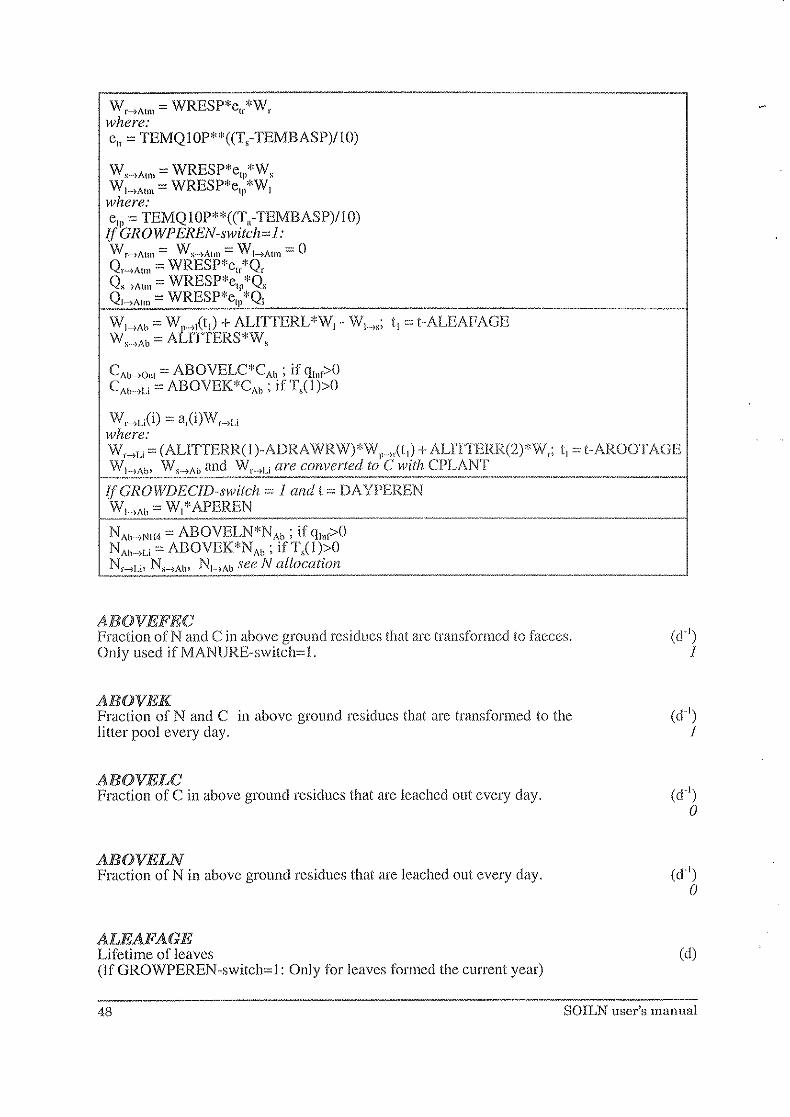
WHAt'" = WRESP*ct/W,. where: c" = TEMQIOP**((T,-TEMBASP)llO)
WHAt'" = WRESP*eq,*W, W I. tAI", = WRESP*ct/,WI where: etp = TEMQlOP**((T,,-TEMBASP)110) If GROWPEREN-switch= 1 : Wr->Atm::::: WS-}A!1l\:::: W1-tAtm:':;:;; 0 Q .- WRESP*e *Q r-)Atm - If r
Q - WRE"SP*e *Q _s---.7Atm - Ip s
QI->Atm = WRESP*eq,*QI
CAIHO"1 '" ABOVELC*CAb ; if qb,r>O CAb.,U '" ABOVEK*CAb ; ifTJI»O
W""'Li(i) = a,(i)W,·._,Ll where: W'_7Li = (ALlTTERR(l)-ADRA WRW)*Wp .. _,,(t l ) + ALlTTERR(2)*W,.; tl "" [·AROOTAGE Wl .. ,Ab, W,_.,Ab and W,· .... 'l; are converted to C with CPLANT
. . ----Kf GROWDEClD-switch = 1 and t = DA YPEREN Wl,Ab = Wl*APEREN
1--'-'-''''------'----·------ --.---.. -.- ------------.. ---NAb .. ,NH4 = ABOVELN*NAb ; if qh,r>O NAb-,Ll = ABOVEK*NAb ; ifTJI»O
~~,Ll' NHAb, Nl .. 'Ab_s_ee_,_N_(_ll_lt_H_.'a_t_io_n __ . ____ ., _______________ , _______ _
AB(JVEFEC Fraction of Nand C in above ground l'csiducs that are transformed to faeces, Only used if MANURE-switch= 1.
(d l)
1
AB(JVEK Fraction of Nand C in above ground rcsidues that arc transformed to the litter pool every day,
AB(JVELC Fraction of C in above ground residues that are leached out cvery day. (d l)
o
AB(JVELN Fraction of N in above ground residues that are leached out every day, (d· l
)
o
ALEAFAGE Lifetime of leaves (d) (If GROWPEREN-switch=l: Only for leaves formed the current year)
48 SOILN user's manual

ALITTERL Fraction of leaf biomass (old biomass if GROWPEREN", 1) lost to litter.
ALITTERR Parameters for root mortality.
ALlTTERR(l): Fraction of daily root growth lost as litter.
ALITTERR(2): Fraction of root biomass (woody biomass if GROWPEREN= 1) lost as litter.
ALI'TTERS Fraction of stem biomass (woody biomass ifGROWPEREN-switeh=l) lost through litter.
AROOTAGE Lifetime of roots formed the current year.
TEMBASP For plant respiration; Base temperature at which temperature effect", 1.
1'EMQ10P For plant respiration. Response to a 10 °C soil temperature change
WRESP Coefficient to multiply the maintenance respiration of root, stem biomass and leaf biomass which is a Q,o function of temperature. The product ofWRESP and the temperature is the fraction of biomass that is lost through respiration. If GROWPEREN-switch = 0: respiration acts on current year biomass. If GROWPEREN-switch = 1: respiration acts on old biomass.
(d')
(-)
(d')
(lr')
(d)
CC) 20
(-) i
(d')
If GROWSTART-switch=l then photosynthesis starts at a certain temperature slim (DA YTAACC, TAACC). Otherwise growth starts at day UPST (see Soil and plant management parameter group).
lfGROWPHEN-switch>O then the date for start of grain development is calculated as a function of temperature and daylength (GRAINI). Grain development starts when an index (i,) becomes Ulllty.
P ARAME'l'ERS 49

= 11 if: t = UPST I, = 2 if: UPST <= t <,= UPET
If GROWSTART-switch= I: i, = ]() if: t>=DA YTAACC t f = t if: l:(,(,-PHOTEMP(I); >0) = TAACC i, = 12 if: t=l f
i, = 2 if: t>lr i, = 13 if: t=DA YPEREN i,. = 0 if: W,=O & t>l72
I~------~------------------'----------------------------------(f' GROWPHEN-switchA): If i, = 2 or i, = 11: ig '" LA" GRAINI(l)*(1 - exp(-x))(l, exp(-y» where: x = GRAINI(4)*(T(t), GRAINI(5»
_Y,--=._G_R_A_IN.--:;I(..c2)""*;:..,(D""(c.:.t),_-_G_R_A_I_N,,,,I(:..;3)c;..) ___ ,----------,---------'
DAYTAACC Day number at which the calculation of T"A", starts
DifYPEREN Day number at which the transformation of assimilates ti'om young pools (current year) to old pools (wood) occur
GRAIN1 Coefficients for the index (i,) which acts as a switch that starls the grain developmcnt.
GRAINI( 1): ThG asymptote ofthe development rate curve. The invcrse value gives the shortest possible duration of the phase in days and is therefore related to the basal vegetative period.
GRAINI(2): Regulates the shape of the development-photoperiod (day length) function.
GRAINI(3): The critical photoperiod (threshold) for the development.
GRAINI(4): Regulates the shape of the development - temperature function
GRAINf(5): Threshold temperature
TAACC Minimum value of the temperature sum (T"A,,) at which growth starts.
6.15 Plotting on Hne
These parameters activates a display of outputs on the screen during the simulation.
PMAX
(d)
(d)
(d')
(h)
CC')
CC)
(nc)
The expected maximum value among the variables selected by XTGD. (--)
50 SOILN user's InHnual

X1'GD Numbers of output variables to be presented on the screen during the simulation. For instance, 4200 means 4 X-, 2 T-, zero G- and zero D variables. X,,, state, T= flow, G= auxiliary and D= driving variables. It is the first variables (of those selected as output) in each array that are plotted.
These parameters are available only if the SPECIAL-switch is ON. They activates special routines not used, or kept fixed, in the original model.
Some of the parameters are used for sensitivity tests. The value for no test is the default value, given in italics. In case both the relative and the absolute value are possible to change a constant value of the variable concerned can be chosen by setting the relative cbange to 0,
TEMPREQ-switch: Alternative temperature response functions for microbial activity may bc used. Also separate temperature response functions could be used for mineralisation-immobilization, denitrification and nitrification. The function is based on a Q,o relation (TEMQ I 0, TEMQ 1 OD, TEMQ ION), with a temperature base (TEMBAS, TEMBASD, TEMBASN) at which the value of the function is one, Below a certain temperature (TEMLIN, '},EMLIND, TEMLINN) the response is linear. This linear function equals the other function at temperature equal to TEMUN, and is zero at Onc.
UTTKCN-switch: CNLITN, CNUTX, CNFECN and CNFECX: 'The specific decomposition rate of litter (UTK) and faeces (PECK) can be set a linear function of the C-N ratio. If the M [CROB-switch is on this option acts on the microbial gross consumption mte (MICK),
MICROB-switch: A special option of SOILN allows you to simulate microbe dynamics. In that case the microbes decompose dead organic material in proportion (MICK) to the amount of microbial biomass. The microbial gross consumption rate is decreased in case of substrate deficiency. At a certain amount of substrate (MICSUB) MICK is half of its maximum value. The microbes daily decomposition can not be more than a certain rnaximum fraction of the substrate (MICMAX). Some of the decomposed material is lost by growth respiration (l-MICEFF) whereas the remaining material increases the microbial biomass. The microbes die off in proportion (MICMORT) to their biomass. This is lost to the litter pool and mixed with dead plant material. The microbes also lose carbon due to maintenance respiration (MICMRESP). Both the mortality and the maintenance respiration rates can be set functions of abiotic conditions. The nitrogen dynamics follows the carbon dynamics. Nitrogen consumed by microbes is the N/C ratio of litter multiplied by the C amounts consumed. Then the C/N ratio of this material decreases due to respiration. The microbes lose N in proportion to their C/N ratio when they die. Depending on if the C/N ratio of microhes is lower or higher than MICCN, the microbes will mineralise N to soil Of immobilise N !i'om soil. In case mineral N is low in soil the microbes N uptake might be smaller than their demand and the microbes can get an increased C/N ratio. You can choose up to three different litter pools on which the microbes acts, litter, humus and an extra littcr pool. The principals are the same for all pools. What differs are the microbial consumption rates (MICK(l-3) from the different pools, the respiration (l-MICEFF(l-3)) and the fraction of dead microbial biomass delivered to different pools (MICMORT(l-3)). The litter fall is separated into the different pools by parameters LITFRACA(l-3) (leaves and stems) and LlTFRACR(l-3) (roots).
A certain fraction ofN deposited and mineral N fertiliser could be directly allocated to the second layer (FERN LA Y2).
The impact of water stress on growth can be modified by parameter PHOETR. CO2 concentration of the air can be given as input affecting radiation use efficiency (C02START, PHOC02).
P AliA.Mg'l'ERS 51

If GROWPHEN-switch=2 then dates for emergency, end of grain filling and harvest are calculated as function of temperature sum (T APHENOL). If temperature sum is low, then date of harvest is determined by a maximum harvest index being achieved (HARINDEXX).
Special options for automatic fertilisation (FERNCALC-switch), an alternative function for calculating photosynthesis (GROWPHOS-switch), mobile ammonium (NH4MOBIL-switch) and automatic correction of certain simulated values (BOUNDARY-switch and parameters BOUN .... ) are activated by switches. For description of the options is referred to the description of switches.
IfFL1?NCALC-switch",1: NAppHF'" '" NApp,-.,Fcn + A VAILN*(Npolup - Nso" .. ,p,,,,,, - x)/UPMA where: x:::: NIllf->No3-N])cr->NH4-NFc11-.. )NH4 I----~~~~~~~~------------------------~----I/FERNCALC-switch=2: N App'-,F", '" N App' ... ,F", + AV AILN - x - y where: x :::: Nlnf.'-)N03"·NDCC.-~NH4-NFert-)NH4 y '" O.2*Nu + 7.yl'HUMK*N" + O.2*Nr+NNH4 + NN03
I/MICROB·switch>O: CA1HU = LITFRACA(l)*CA"._,I.'To, C, .. ,u '" LITFRACR(l)*C, .. "xl'>" D:off)r Nitrogen give: NAI>,u, N, .. ,u D:ofor flumu.\' give: CAh--)h) Cr ... "h) l'-IAh ... )h' Nr ... >,h
D:ofor Litter2 give: C/\/J--)U2 I Cr--->U2, NAb.--~Jj2) Nr--}U2
CI.' ... '''''~ MICK(l)*(,,,,,*e,e,,,C,,, ; <=MICMAX*Cu C", .. ,u '" x*MICMORT(l)*C", where: fs"" ,= C,j(CI.,+MICSUB(1)) x ,= abiotic facior, see below D:ofor Humus give: C""", C", ... ,,, /):0/01' Litter2 give: CU2 --->/I!) CIIHU2
[fM/CROB·switch >=1 >=1 >=1 =2 or 3 =3
>=1 >=1
=2 or 3 ,,=3
C"HA'", = (l -MICEFF(l ))Cu ""+(1-MICEFF(2))CI.i2.""+(1-MICEFF(3))C,,_,,,, + y*MICMRESP*C",
where: y '" abiotic factor, see below
52 SOILN llser's manllal

NLi .-m1 ::::: CI.i->mNljCLi >=1 Nm ... )Li ::::: Cm .... }]jNn/Cm >=1 D:o for llufnus give: N Il ._.)!/!, N/II._.>h '~2 or 3 D:ofor Litter2 give: Nri2-.. tlll' Nm .... ,U2 =3
N",(new) = C",(new)/MICCN implies: where: C",(ncw) '" C'" + LlC", LlCm ::::: CLi'-)1ll+CLi2_H\l+,Ch._.)m-(CIll __ )U+Cm .. _rLi2+Cm_,h)-Cm ... ->A!1ll
Nn/new) ;:;:;:; Nm + LlNmJ .. Nm.~.)NH4 LlNml == NLi-->11l+NLi2 __ ->m+Nh ... ->m-(Nm._.)Jj+Nm_0Li2+Nm .. _>h) Nm-)NH4 ::::::: -«C",+LlC",)/MICCN - (N",+LlN",,)) ; < UPMA *(NN03+NNH')
Nh.,N"4 = see Mineralisation and immobilisation =4 C'HA''''"' CNORG*Nh .,NH4 =4
-If MICABIO··switch>O: IfMICABIO-switch: mortality abioticjilcior x", c, =1 m.ortality abiotic factor x ,~C'" =2 maintenance respiration abioticfcu:tor y ,= c, =3 maintenance re,lpiration abiotic factor y = =4 combinations are multiplication"of'e, and e",::/J x = c,c", >=12
IfTEMPREQ-switch=J: c, = T/fEMUN*TEMQI0**«TEMUN·TEMBAS)/10) ; ijn<7EMLlN If'TEMPREQ-switch=c2: c, '" (T/rEMMIN)lcrEMBAS-TEMMIN)2 IfTEMPREQ-switch=J: c, = TEMPOL(1)+TEMPOL(2)*T,+TEMPOL(3)*T/+TEMPOL(4)*T,'+"",
IfGROWPHOS.switch=l: W A'",.,p = PGRESP*2:(LlA,(xPM"/(x+(I .. PTRANSl\1)*PM,,,) where: x = PHOEFF*EXTCOEF*l*cxp(-EX'fCOEF*2:L1/I.,) PM,,, = PMAX20( 1 )*( I-PMAX20(2)*( l-exp( -EXTCOEF*2~i\A,»*fl*Daylength ... ".'-~--.".---.-~----~~.""-------
IfLlnXCN-switch =,] or 3: UTK(new) = UTK*(1-(C,jN,j - CNLITN)/(CNLlTX ... CNLITN») and MICROB .. switch >0: MICK(ncw) '" MICK(1)*(1-(C,/NLi •· CNLITN)/(CNLITX ... CNUTN)) +D:ofor Humus and Litter2 (MICK(2) and MICK(J))
IfLl7TKCN·switch =2 or J: FECK(new) = FECK*(l-(C,IN, - CNFECN)/(CNFECX - CNFECN))
If' GROWPHEN-switch=2: i" = 1 if: 0 < ig < 1 , _ if =(2:('1'.:.- r APHENOL(l);>O»)/TAPHENOL(2) 1, - 1 If. I" - 1 i, = 2 if: 1 < ill < 2 i, '" 21 if: 2<= ig < 3 . ii =,(2:(T,,-TAPHENOL(3);>O»)lTAPHENOL(4)+2 1, = 2 If: 3<= I" < 4
ig =, (2:(T,,-TAPHENOL(5);>O))/TAPHENOL(6)+3 i, = 3 if: i" = 4 or W/(Wg+W,+WJ > HARINDEXX
If'ROOl1JENS-parameter>O: UPMA(ncw) = UPMA*(W,(i)/oz(i)/ROOTDENS)**ROOTDENSE
PARAMETERS 63

IfNH4MOBIL-switch=1: NNH'I(O--+(i+') '" Cjw(i)l1N1"'(i)/l 000 (i,.c!ayer) where: nNI14(i) '" NNH4so'(i/0ITHlCK(i) ; 0>=0" \vhere: NNH4So!(O ;::: NNH4(i),·NNI-14Ads(i)
where: NNH4Ad'(i) '" x + y*NN"'4(i) where: NNH4Ad,[gN/gSoil] '" NH4ADSA + NH4ADSB*nNI14[gN/m3Water] implies: x '" NH4ADSA(i)/(I/BULKDENS(i)ITHICK(i)+NH4ADSB(i)/0/THICK(i)) y = l/(0/BULKDENS(i)/NH4ADSB(i)+1)
fw'" PHOETR(1)+PHOETR(2)*E/EtP .~~L _____________________________ • ___ ___
if C02START> 0: C02Atm = C02START*(l+C02INCY*(Year since simulation start)) PHOEFF(new) = x*PHOEFF; where x '" I+PHOC02"'(C02Atm-C02REF)/C02REF
AlWOTE Coefficients for root development as function of transpiration ratio. NOTE! Depend on GROW AEQ-switch, For explanation of coefficients see GROW AEQ, Independent variable is: x" j·AROO,!'ETR*E/Etp.
AROOTE(l): Coefficient a
AROO'T'E(2): Coefficient b
AROOTE(3): Coefficient c
AlWO~l'E'l'R Relative change of the transpiration ratio in the root allocation function,
AlWO'l'NI Coefficients for root development as function of leaf N concentration. NOTE! Depend on GROWAEQ-switch. For explanation of cocfficients see GROW AEQ. Independent variable is rc1ative leaf N concentration (x=(n,-NLEAFN)/(NLEAFXG-NLEAFN)). "Other equation" is: 1+ AROOTN-( 1-( (NLEAFXG-n,)/(NLEAFXG-NLEAFN)2)05. where n, is N concentration of leaves (N,IW,). If GROWPEREN", 1 then n, is both current year and old leaves. If SPECIAL-switch=1 then: If AROOTNI(l)<O then n, is replaced by N concentration of newly formed leaves (n,'=N,'/W,'). If GROWPEREN=! then n, is now only the current year old leaves. (The absolute value of AROOTNI(l) is used)
AROOTNI(l): Coefficient a
AROOTNI(2): Coefficient b
AROOTNI(3): Coefficient c
(-)
(differ)
(differ)
( -) 1
(-)
( differ)
(differ)
54 SOILN u801')8 manual

AROO'1W Coefficients for root development as function of total plant biomass. NOTE! Depend on GROW AEQ-switch. For explanation of coefficients see GROW AEQ. Independent variable is total plant biomass (x=W,). No "other equation" is available.
AROOTW(I): Coefficient a
AROOTW(2): Coefficient b
AROOTW(3): Coefficient c
AVlULN When simulating N fertilisation: If FERNCALC-switch=l then A V AILN is the fraction to multiply to the estimated supply (unit is -). It' FERNCALC-switch=2 then A VAILN is the wanted soil mineral N (gN m·2
).
BOUNF'l'O'l' Total number of variables (including error variables) in the file nsed for correction. Only used if BOUNDARY.·switch '" 1,2 or 3
BOUNRERR Relative error of variables used for correction. If BOUNRERR<O then equal to the absolute error. Only used if BOUNDARY -switch=3
BOUNVALU Value that simulated variable should be corrected to in each time step. Value = ··99 is treated as missing. Index I-max20. Only used if BOUNDARY-switch=4
BOUNVNUM Variable number of simulated variable that should be corrected during simulation. Numbers are listed in Appendix 1. States variables (X-vm-): X(n) where n=BOUNVNUM Flow variables (T·var): T(n) where n=BOUNVNUM-IOOO Auxiliary variables (G-var): G(n) where n=BOUNVNUM-10000 Index I-BOUNFTOT/2 Only used if BOUNDARY -switch> 0
BULKDENS Bulkdensity of soil. Index 1-10: Soil layer. Below layer 10 the value of layer 10 is used. Only used if NH4MOBIL-switch = 1.
CNFECN Minimum CoN ratio of faeces at which no decomposition occurs. Only used i LlTTKCN switch=2 or 3.
PARAMETERS
(-)
(differ)
(differ)
(differs) J
(-) 2
(-) 2
(differ) ·99
(-) o
(g m") O.Je+6 1.0e+6
(-) ()
55

CNFEtL:K Maximum C-N ratio of faeces at which maximum decompositiou occurs. Only used i LlTTKCN switch=2 or 3.
CNLITN Minimum C-N ratio of litter at which no decomposition occurs. Only used i LlTTKCN switch=1 or 3.
CNLI'lX Maximum C-N ratio of litter at which max.imum decomposition occurs. Only used i LlTTKCN switch=l or 3.
C02INCY Annual relative incremcnt of atmospheric CO2 conccntration. Not used if C02START= 0
C02REl7 Atmospheric CO2 conccntration at which the radiation use efficiency equals the onc given by pararncl:cr PHOEFF.
C02START Conccntration of carbon dioxide in the atmosphere al start of simulation. =, o implies option is cancelled. Normal value is about 350
Ji'ERNLAY2 FERNLAY2( I): Fraction of dissolved ammonium N from solid fertiliser that is allocated direclly to the second layer (N"''''',NII4)
FERNLAY2(2): Fraction of amnl0niuDl N deposition and ifiltrated nitrate that is allocated directly to the second layer (N!),p.~'N'I4' N'''r .... ,No:I) .
I1ARJNJiJEXX Maximum harvest index ((grain biomass)/(tot above ground biomass». Only used if GROWPHEN-switch = 2.
LITFRACA Fractions of leaf and stem litter delivered to (index 1-3) Litter, Humus and Litter2, respectively. Only used if MICROB-switch>O
LI'l'FRACR Fractions of motlitter delivered to (index 1-3) Litter, Humus and Lilter2, respectively. Only used if MICROB-switch>O
,
(- ) o
(-) o
(-) o
(i') O.OJ
(ppm) 350
(pp m) o
(-) o
() o
(-) 0.6
(-) 1,0,0
(-) J,O,O
56 SOILN user's 111unual

lVlICCN C-N ratio of microbes. Only used i MIC ROB switch>O.
MICEFF Efficiency of the internal synthesis by microbial biomass of organic material from (index 1-3): Litter, Humus, Litter2 Only used if MICROB-switch>O
MICK Microbial gross consumption rate per unit of microbial biomass, at a reference temperature and optimal soil water condition. The value differ depending of type of substrate. Index 1-3 refers to substrate: Litter, Humus, Litter2. Only used if MICROB-switch>O
MICMAX Maximum fraction of substrate decomposed every clay. Only used if MICROB-switch>O.
MICMORT Microbial relative mortality rate. Index J -3: Litter, Humus, Littcr2. Only used if MICROB-switch>O.
MICMRESP Fraction, at a reference temperature, of microbial biomass lost by maintenance respiration. Only used if MICROB-switch>O.
MICSUB Substrate amount at which MICK is half of its maximum value. Index ] .. 3: Lilter, Humus, Littcr2. IfMICSUB(1 )<0: fs"" "" C,)(CLi-MICSUB( 1 yc",); the same for index 2 and 3. Only used if MICROB-switch>O.
NH4ADSA Coefficient (a) in the relation between ammonium in soil solution and amount adsorbed on soil particles: NNH4Ad, (gN/gSoil) "" a + b * NNH4so' (gN/m'Water). Index ]·-10: Soil layer. Below layer 10 the value of layer 10 is used. Only used ifNH4MOBIL-switch = 1.
NH4ADSB Coefficient (b) in the relation between ammonium in soil solution and amount adsorbcd on soil particles: NNH4Ad, (gN/gSoil) '" a + b '" NN"4S,,' (gN/m3Water). Index 1-10: Soil layer. Below layer 10 the value of layer 10 is used. Only llsed if NH4MOBIL-switch "" 1.
PARAMETERS
(-) .5
(-) 0,0,0
(cl") 0.1
(-) 0,0,0
(d') o
C)
(gN gSoir') O.5e-6
(m3Water gSoir') 2.0e-6 O . .5e-6
67

OUTLAY (i) Layer. The abiotic response function is calculated for each layer but is stored as output only for this layer. A value outside 1- JO will give you the average response function for all layers as output.
OUTLITCN Switch selecting for which pool the specific decomposition rate should be stored in the auxiliary variableLITKCN. 112/3: Litter, Humus, Litter2. Layer for which it should be stored is selected with parameter OUTLAY.
OUTRATCN Switch selecting for wbich pool the C/N ratio should be stored in the auxiliary variable RATCNL. 112/3/4: Litter, Humus, Litter2, Microbes.
OUTSW Switch selecting which internal model should be stored in the auxiliary variable SWITCHOUT. 112/3/4: Swflush, Swstart, Swplough, Swbarv.
PIWC02 Relative increase in radiation use efficiency due 10 doubled atmospheric CO2 concentration.
PIIOE'l'R Coefficients modifying the effect of transpiration ratio on plant growth.
PHOETR(l): a in eq. fw=a+b*E/E,p
PHOETR(2): bin eq. f~v=a+b*E/E,p
PPMAX20 Coefficients for maximum photosynthetic rate, Only used if GROWPHOS-switch = 1.
PPMAX20(l): Maximum leaf photosynthesis rate at optimal temperature, water and uitrogen conditions (note area refers to leaf area).
PPMAX20(2): Rate of decline of maximum leaf photosynthesis with increased leaf area index.
PTRANSM Leaf transmission coefficient. Only used if GROWPHOS-switch = I,
PGRESP Growth conversion efficiency (reductiou coefficient of canopy photosynthesis due to growth respiration). Only used if GROWPHOS-switch = 1,
(-) 1
(-) 1
(-) 1
H J
o
j
(kgC02 ha- 1 h- 1)
43.2
(-) 0.35
(-) 0,1
(-) 0.83
58 SOILN user's manual

ROOTDENS Parameter making root uptake (UPMA) equal a function of root dens ity. Only used if ROOTDENS > O.
ROOTDENSE Parameter making root uptake (UPMA) equal a function of root density, see parameter ROOTDENS.
SLEAFND Number of days before the current day of which the leafN deficit should be added to the leaf N demand.
SROOTND Fraction of the accumulated root N deficit during the current year that should be added to the root N demand.
SSTEIVlND Fraction of the accumulated stem N deficit during the current year that should be added to the stem N demand.
TAPI-lENOL Temperature limits for phenologic functions. (index= 6) TAPHENOL(I): Threshold temperature for calculating day of emergency. ("C) TAPHENOL(2): Accumulated temperature sum since day of sowing to day for emergency. (day"C) TAPHENOL(3): Threshold temperature for calculating day of cnd of grain filling. Cc) TAPHENOL( 4): Accumulatcd temperature sum siuce day for start of grain filling to day for stop of grain filling. (day"C) T APHENOL(5): Threshold temperature for calculating day of harvest. Cc) TAPHENOL(6): Accumulated temperature sum since day for end of grain filling to harvest. (day"C) Only used if GROWPHEN-switch = 2.
TEIVlBASD For the denitrification process; Base temperature at which temperature effect = 1. Only used ifTEMPREQ-switch=4, 14 or 24.
TEIVlBASN For the nitrification process; Base temperature at which temperature effect = 1. If TEMBASN = 0 then TEMBASN is set equal TEMBAS. Only used ifTEMPREQ-switch=4, 14 or 24.
P ARAME'l'ERS
(gDW nl') o
(-) 1
(d) o
(-) o
(-) ()
differs
(c) 20
(C) 20
59

TEMLIN For the mineralisation-immobilisation process, Threshold temperature below which the temperature response is a linear function of temperature, Only used if TEMPREQ-switch= I,
TEMLIND For the denitrification process, Threshold temperature below which the temperature response is a linear function of temperature, Only llsed if TEMPREQ-switch=4 or 14,
TEMLINN For the nitrification process, Threshold temperature below which the temperature response is a linear function of tenlperaturc, Only used if TEMPREQ-switch=4 or 14,
7l'EMMIN Minimum temperature for microbial processes in the Ratkowsky function, Only used if TEMPREQ"switch=2 or 24
TEMMIND '1'he same as for TEMMIN but for the denitrification process, Only used if TEMPREQ-switch=24
TEMMINN The same as for TEMMIN but for the nitrification process, Only used if TEMPREQ-switch=24
'PEMMlP'OL Cocfficients in a 6-degrcc polynornialicmperaiUl'C function, Index ]·7, Only used if TEMPREQ-switch=3
TEMQ10D For the denitrification process. Response to a 10 'C soil temperature change, Only used if TEMPREQ·switchooA or 14,
'l'EMQHflN For thc nitrification process, Response to a 10 'C soil temperature change, Only used if TEMPREQ-switch=4 or 14,
(0C) 5
("C) 5
(0C) 5
("C) ··8
(OC) ,,8
(differ)
(-) 3
(-) 3
GO SOILN 11801')s manual

7 OlJTPlJTS Output variables arc stored in a PG-structured file named SOILNnnn.BIN where nnn is the current nm number. Also, a list of output variables are found in the summary file named SOlLNnnn.SOM. The variables to be stored in the summary file can be selected by the switch LISALLV.
The output variables arc divided into four categories: states (coX), flows (=T), auxiliaries (=G) and drivings (=oD).
Symbols given in brackets refer to Eckersten (1991a) and Eckersten & Jansson (1991).
All variables denoted ACC .... arc used only to check output and not involved in the model calculations.
Vadahle
ACCBAL
ACCBALC
Nitrogen mass balance check of ACC ... -variablcs (Input-Ou tput-Store)
Carbon mass balance check of ACC ... C·variables (Input·Outpul-SWrc)
ACCJ)JENI Accumulated denitrificatio!l of N03-N
ACCJ)JEIP Accumulated N deposition
ACCJ)JLOSS Accumulated leaching ofN03-N
ACCFER'1' Accumulated N fertilisation, other than manure and deposition
ACCIIA.RV Accumulated N harvested
ACCIIARVC Accumulated C harvested
ACCMAN Accumulated N fertilisation through manure
ACCPIlOSC Accumnlatec! C uptake by net photosynthesis
ACCIP LAN'1' Accumul ated change in total plant N
ACCPLAN'1'C Accumulated change in total plant C
ACCRESPC Accumulated C lost by respiration from plant and litter
ACCSOIL Accumulated change in soil N
ACCSOILC Accumulated change in soil C
CF (Cr) Faeces C-pool (Index= layer] to 2; two uppermost layers)
OUTPUTS
(gN m')
(gC 1112)
(gN m 2)
(gN m 2)
(gN m·2)
(gN m 2)
(gC m·2)
(gN nf2)
(gC m·2)
(gN m 2)
(gC m 2)
(gC m 2)
(gN m·2)
(gC m·2)
(gC m·2)
61

CIl (C,,) Humus C-pool (Index=laycr I to min(NUMLAY,lO))
CL (Cu) Litter C-pool (Index=layer I to min(NUMLAY,IO))
CL2 (CU2) Intermediate litter C-pool (litter2) (Index=\aycr I to min(NUMLA Y,IO))
CM (Cm) Microbial C-pool (lndex=layer I to min(NUMLA Y, I 0)) (if SPECIAL=l)
FERT (N"",) Solid fertilizer N-pool (nndissolved)
GRAlNN (N,) Grain N-pool (PLANT)
Gl?A1NW (Wg) Grain dry weight (PLANT)
LEAFN (N,) Leaf Npool (PLANT)
LEA.FW (W,) Leaf dry weight (PLANT)
LI'J['AJB,OVl£ (NA,,) Plant residue N-pool, above ground
LlITA.BOVl£C (CA") Plant residue C-pool, above ground
.NF
NIl
NIl4
NUT
NLIT2
NM
N03
IWOTN
ROOTW
STEMN
STEMW
WLEAFN
62
(N,) Faeces N'pool (lndex= layer I to 2)
(N,,) Humus N·pool (llldex=layer I to mill(NUMLA Y,IO))
(NN'''') Ammonium NH4-N pool (Indcx= layer I to min(NUMLAY,lO))
(N,J Litter N·'pool (Index=layer I to min(NUMLA Y,IO))
(Nu,) Intermediate litter N-pool (litter2) (Index=layer I to min(NUMLA Y,IO))
(N",) Microbial N-pool (Index=layer 1 to min(NUMLA Y,IO)) (if SPECIAL=l)
(NN03) Nitrate N03-N pool (Index= layer I to NUMLA Y)
(N,.) Root,N (PLANT)
(W,) Root dry weight (PLANT)
(NJ Stem-N (PLANT)
(WJ Stem dry weight (PLANT)
(N"J N in old leaves (if GROWPEREN=I)
(gC nf')
(gN m")
(gN m')
(gDW m")
(gN rn')
(gDW m')
(gN rn'2)
(gC 111')
(gN m')
(gN m')
(gDW nf')
(gN m')
(gDW Ilf')
(gN m'2)
SOILN user's manual

WLEAFW
WIWOTN
WROOTW
WS'l'EMN
WS'l'EMW
XAVAlN
XAVAlW
Variahle
AAVAIIPW
AAVAlUN
ALEAFAN
ALEAPA.W
ALEAli'GN
ALEAFGW
ALEAFN3N
ALEAFLlN
ALEAFLlW
ALEAFSN
ALEAl?SW
ALEAFWN
AS'l'EMWN
ALEAFWW
APHOTLW
OUTPUTS
(W,,,) Biomass in old leaves (older than one year, normally) (if GROWPEREN= I)
(N,w) N in old roots (if GROWPEREN= 1)
(W,w) Biomass in old roots (if GROWPEREN=l)
(N",) N in old stems (ifGROWPEREN=])
(W",) Biomass in old stem (if GROWPEREN=d)
(N,,) N in plant available for re-translocation (if GROWPEREN= 1)
(W,,) Assimilates in plant available for growth (if GROWPEREN= 1)
(Symllol) Explmmtiml
(W"'j» Biomass flow: From available pool to growth (added to PliOS but not included) (PLANT)
(N,,_,uC') N flow: From available pool to growth (added to TOTUPT but not included) (PLANT)
(N,_,,,) N flow: From leaf to available pool (PLANT)
(W,_",) Biomass flow: From leaf to available pool (PLANT)
(N,. __ ",) N flow: From leaves to grains (PLANT)
(W,_,,) Biomass flow: From leaf to grain (PLANT)
(N"",]+"",.,.) N flow: Leaches from leaf to nitrate infiltration (PLANT)
(N'.'Ab) N flow: Leaf litter (PLANT)
(WI->Ab) Biomass flow: from leaves to above ground residues (PLANT)
(N,..,,) N flow: From leaf to stem (PLANT)
(W,_,,) Biomass flow: From leaf to stem (PLANT)
(NH,w) N flow: From leaf to olelleaves (PLANT)
(N,,,w) N flow: From stem to woody stems (PLANT)
(W'_,'w) Biomass flow hom leaf (0 old leaves (PLANT)
(Wp._,') Daily gross leaf growth (PLANT)
(gN m-2)
(gDW m-2)
(gN m-2)
(gDW m-2)
(gN m-2)
(gDW m 2)
(gDW m' er')
(gN Ill' tI')
(gDW m-' d-')
(gN nI' cl')
(gDW m-2 cri)
(gN m-2 cri)
(gN nf' el-')
(gDW nf' ell)
(gN m-2 cr')
(gDW m-2 cri)
(gN nf' cri)
(gN m-' cr')
(gDW m-' cr')
(gDW 111-2 d-')
63

API10TRW (Wp ... .,,) Daily gross root growth (PLANT) (gDW nf' cri)
APIlOTSW (Wp.,J Daily gross stern growth (PLANT) (gDW rn' cri)
AROOTAN (N, .. ,,,) N flow: From root to available pool (PLANT') (gN rn' cl')
AROOTAW (W,.,,,) Biomass flow: From root to available pool (PLANT) (gDW m,2 cl'l)
AROOTGN (N"",g) N now: from root to grain (PLANT) (gN m" cl")
AROOTGW (W"",g) Biomass flow: from root to grain (PLANT) (gDW m,2 cl")
AROOTLIN (N,'Li) N flow: Root litter (PLANT)
AROOTLIW (W,.,I.;) Biomass flow: from root to litter (PLANT)
(gN m' cl')
(gDW 111,2 cl")
AROOTSN (N, .. ,J N flow: ti'om root to stem (PLANT) (gN m" cl")
AROOTSW (W,.,J Biomass flow: from root to stem (PLANT) (gDW m 2 cl")
AROOTWN (N,·,»w) N flow: From root to woody roots (PLANT) (gN Ill" cl")
AR007rWW (W,.»,,) Biomass flow: From root to woody roots (PLAN'I') (gDW m' cri)
ABOILGN (Ns";],,J N flow: From soil to grain (PLANT) (gN rn" cl")
ASOIILLN (Ns,,;],,) N flow: From soil to leaves (PLANT) (gN m' r]')
ASOILRN (Ns"u.") N flow: From soil to root (PLANT) (gN m" cl")
ASOILSN (Ns"u,,) N flow: From soil to stem (PLANT) (gN m" ell)
ASTEMAN (N",,,) N flow: From stern to available pool (PLANT) (gN In' cl")
AS1'EIVlAW (WH ,,) Biomass now: From stem [0 available pool (PLANT) (gDW m' cl')
AS'l'EMGN (N, ... ,,,) Nitrogen flow: From stem to grain (PLANT) (gN m" d")
AS1'EIVlGW (W",.,,,) Biomass flow: From stem to grain (PLAN]') (gDW m' cl")
ASTEMLIN (NHAb) N flow: (N;(ut)) Stem litter (PLANT) (gN m" d')
ASTEMLlW (W>-;Ab) Biomass flow: from stem to above ground residue;; (gDW m' d') (PLANT)
AS't'lt:1VfWW (W,;;w) Biomass flow: From stem to woody stems (PLANT) (gDW m,2 cri)
AWLEAFLIN (N'w.,ij) N flow: From old leaf to litter (PLANT) (gN m,2 cl")
AWLEAFLN (N,w-c>') N flow: From old leaf to young !caf (PLANT) (gN Ill" d")
AWLEAFLlW (W'w,u) Biomass flow: From old leaf to litter (PLANT) (gDW nf' cl")
A.WLEAFLW (W'w.,') Biomass flow: From old leaf to young leaf (gDW nf' cl") (PLANT)
SOILN user's manual

AWLEAFN8N (N'w-''',f+s",..) N flow: Leaches from old leaf to soil nitrate infiltration (PLANT)
AWLEAFAN (N,w_,,,) Nitrogen flow: From old leaf to available pool (gN m-2 d- ') (PLANT) (Not amonng outputs yet)
AWLEAFAW (W'w-;,,) Biomass flow: From old leaf to available pool (gDW m-2 d- ') (PLANT)
AWSTEMAN (N"H") Nitrogen flow: From old stem to available pool (gN m-2 d- ') (PLANT)
AWS'l'EMAW (W,w_,") Biomass flow: From old stem to available pool (gDW m-2 d- ') (PLANT)
AWROOTAN (N,w,") Nitrogen flow: From old root to available pool (gN m' d ' ) (PLANT) (Not amoung outputs yet)
AWROOTAW (W,w_,,,) Biomass flow: From old root to available pool (gDW m-2 cri) (PLANT)
AWROOTLIN (N,w"J N flow: From woody root to litter (PLANT) (gN m' d- ')
AWROOTLlW (W,w_,'';) Biomass flow: From woody root to litter (gDW m-2 cl-') (PLANT)
AWSTEMLIN (N",_'AI.l N flow: From woody stem to litter (PLANT) (gN m' cl ')
AWS'I'EMLIW (W,,,_,Ab) Biomass flow: From woody stem to litter (gDW m-2 d ') (PLANT)
CFLOSS C flow: Faeces mineralisation + humification (gC m-' cr') (lndex= layer] to 2)
CHAl?,V (C"'''''I_,II",,) C flow: Harvest export of plant-C (PLANT) (gC m-' cri)
CLLOSS C flow: Litter mineralisation + humification (gC m-2 cl-') (CLMIN+CLHUM) (Inclex= layer 1 to min(NtJMLA Y, 1 0))
CLMIC (CI,;-;",) C flow: Microbial gross consumption of litter (gC m-' cl-') (Index=layer)
CL2MIC (Cw._,,,,) C flow: Microbial gross consumption of litter2 (gC m-2 cri) (Inclex=layer)
CHMIC (Ch_,,,,) C flow: Microbial gross consumption of humus (gC m-2 cl-') (Index=layer)
CHMIN (Cb-,AI"') C flow: Loss from humus by respiration (gC m-2 cl ') (Index=layer). Only used if MICROB-switch=4
CLROFF (CLi-,Sn'""n) C flow: Loss oflitterin uppermost layer to stream (gC m-2 cl-') due to surface runoff (however included in ACCRESPC).
CM LIT (C",_",;) C flow: Microbial loss to litter (Index=layer) (gC m-2 cl-')
OUTPUTS 65
CMLI1'2 (Cm~>W) C flow: Microbial loss to liltcr2 (Indcx=laycr)
CMHUM (Cm.>h) C flow: Microbial loss to humus (lndcx=layer)
CMMIN (Cm>A,m) C flow: Microbial loss due to growth and maintenance respiration (Index=layer)
DECACF (CAb>!) C flow: Above··ground residue to faeces pool CP(1) ifT,(l) > 0, Only used if MANUREswitch=1.
DECACLI1' (CAb>l.;) C flow: Above~ground residue to litter CL(l), Only used if MICROR·switch,=!
DECACLI2 (CAh>W) C flow: Above,·ground residue to litter2 CL2(l)
DECACHUM (CAb ->,,) C flow: Above~ground residue to humus CH(l)
DECALEAC (CAb.>O",) C flow: Losses of above·ground residue to boundary through leaching
DECALEAN (NAh->NH4) N flow: Leaching of above~ground residue to soil arnmonium N114( 1)
DECALIT (NAb.>'iT,,') N flow: Above··ground residue to litter NL( J), If MICROB·switch= 1 then DECALlT is split up into flows to different pools,
DECALI1'C (CAb,U'\>t) C flow: Above··ground residue to litter CL(1), If MICROB~switch=llhcn DECALITC is split up into flows to different pools,
DECAIVF (NAb>') N fiow: Above~ground residue to faeces pool NF(l) if T,(l»O. Only used if MANUREswilch=cl,
DECANLI't (NAh~>',;l N flow: Above~groutld residue to litter NLJT(l), Only used if lllrICROB-switch"d
DECANLI2 (NAh>W) N flow: Abovc~gr(]und residue to Jitter2 NUT2(l)
DECANHUM (NAb->b) N flow: Above~ground residne to humus NH(l)
DECAJU)FF (NAh.->SU''''''') N flow: Loss of above ground residue to stream due to surface runoff
DECAROlf?FC (CAb.;O",) C flow: Loss of above ground residue to stream due to surface runoff (however included in ACCRESPC),
DENI (NN03-,A,m) N flow: Denitrification of N03 (Index= layer 1 to min(NUMLA Y, 10))
DEPOLEAF (Nn,p~,,). N flow: Dry deposition absorbed by leaves, (PLANT)
DEPONIl4 (N ) N !'lc)w' DC'[)C)S'I'tl'C)n (wet alld dry) to soil n,p,NH4 ' ammonium NH4(l)
(gC rn' d·')
(gC m·2 d')
(gC m 2 cr')
(gC m-2 cr')
(gC m·2 d")
(gC m-2 cr')
(gN m-2 li')
( N ·2 I·') gIll· C.
(gC m 2 d')
(gN m 2 cr')
(gN m' cf')
(gN nf2 cr')
(gN m·2 d·')
(gN m 2 cr')
(gC m·2 cr')
66 SOILJ.'J uscr)s manual

lDEPONO:Ji (N"gp-,hMSm,) N flow: Deposition of nitrate to soil (wet and dry)
lDEPOWLEJiF (N",!",w) N flow: Dry deposition absorbed by old leaves. (PLANT)
lDLOSS
FER1'1N
FI!.NCB
FI!.NNA
FINNB
FI!.NNH
J?NI!.T
HARVGN
HARVGW
.HARVLN
JJlARVP~W
HJll~VSN
HARVSW
INCALl1'
JNCALJTC
NEWCL
NEWCLLJT
NEWCLLI2
(NN030S"",m) N flow: N03 leaching to tiles (Index= layer 1 to NUMLAY)
(NAPP""'!'''') N flow: Addition of solid fertilizer N
(CA!,P"') C now: Carbon in faeces in manure to faeces (Index= layer 1 to 2)
(NApP"'.;) N flow: Nitrogen in bedding in manure to litter (lndex= layer 1 to 2)
(NApP"'.) N flow: Nitrogen in faeces in manure to faeces·N (lndex= layer 1 to 2)
(NAI,p"N"") N flow: Nitrogen in NH4 in manure to NI-HO (Inc ex= layer I to 2)
(NN"4,N03) N flow: Nitrification of NH4 to N03 (Index= layer 1 to min(NUMLAY, 10))
(N" ... ,,,,,,,.) N flow: harvest of grain (PLANT)
(Wg .. ,'h,J Biomass flow: harvest of grain (PLANT)
(N"H""') N flow: harvest of leaves (PLANT)
(W, .. ",,,,J Biomass How: harvest of!caves (PLANT)
(N,.",,,,,) N flow: harvest of straw (PLANT)
(W",,,,,,.) Biomass flow: harvest of straw (PLANT)
(NI""'''';Ab) N flow: Plant to above-ground residue
(Cl""''' ,Ab) C flow: Plant to above-ground residue
(C, ... ,uro,) C flow: Incorporation of root carbon or above-ground residues to litter-C (lndex=layer). If MICROB-switch=l then NEWCL is split up into flows to different pools.
(C, ... ".;) C flow: Root to litter. (lndex=layer). Only used if MICROB-switch= 1.
(C, . .,uz) C flow: Root to litter. (Index=layer)
NEWCLHUM (C, .. )u) C flow: Root to litter. (lndex=layer).
OUTPUTS
(gN rn" cl")
(gN m-2 d")
(gC m-2 cl")
(gN nf' cl")
(gN rn' cr')
(gN ill" cr')
(gDW m' cr')
(gN m·l cl")
(gDW m" cl')
(gN m" cl')
(gDW m" cl")
(gN m-2 cr')
(gC nf' cr')
(gC m-' cr')
(gC m" cr')
67
NEWNL (N,",UTot) N flow: Root to litter (Index=layer). If MICROB-switch=1 then NEWNL is split up into flows to different pools.
NEWNLLIT (NH !.;) N flow: Root to litter (Index=layer). Only used if MICROB-switch= I.
NEWNLLI2 (N,_,w) N flow: Root to litter2 (Index=layer)
NEWNLI:IUM (N,"",,,) N flow: Root to humus (Index=layer)
NFERTNI:I4 (NFCtt ,NH4) N flow: Solid fertilizer N dissolved to soil ammonium NH4(l)
NFERTN03 (NF,",!t"+s,,,cJ N flow: Solid fertilizer N dissolved
NFI:IUM (N'"0") N flow: Humification of faeces-N to humus""N (Index= layer I to 2)
NFLOW (NN03OJ",N030+'») N flow: NOrN flow to the layer below (Index= layer 1 to NUMLA Y -I)
NFMIN (N"NH4) N flow: Mineralisation offaeees-N to NH,,-N (Index= layer I to 2)
NIl4DLOSS (NN'"I4,'''"",,) N flow: NH, leaching to tiles (Index= layer J to NUMLAY)
NIl41i'LOW (NNH'O)-",NH4(i+'») N flow: NH,-N flow to the layer below (Index= layer 1 to NUMLA Y -I)
NIlARV (Np"""""",,,,"J N flow: Harvest export of plant-N (PLANT)
NIHIMllC (N"",,) N flow: Microbial gain from humus
NIlMIN (N"-)NH4) N flow: Mineralisation of humus-N to NH4-N (Index= layer 1 to min(NUMLAY,IO))
NLIlUM (NLi_),) N flow: Humification of litter-N to humus-N (Index= layer I to min(NUMLA Y, 1 0))
NLMIC (Nu _)",) N flow: Microbial gain from litter
NL2MIC (N,.ih,,) N flow: Microbial gain from litter2
NLMIN (NU -)NH4) N flow: Mineralisation(immobilisation) of!itter-N to NH4 (Index= layer Ito min(NUMLA Y,IO))
NLROFF (Nu""""""",,,,) N flow: Loss of litter from uppermost layer to stream due to surface runoff
NMIlUM (N"H") N flow: Microbial-N to humus (Index=laycr)
NMLIT (N",)!.;) N flow: Microbial-N to litter (Indcx=layer)
(gN Ill"' d"')
(gN Ill"' cl"I)
(gN IIl' c\"')
(gN m"' cl")
(gN m' d')
(gN m"' cr')
(gN m"' cr')
(gN m"' d"')
(gN m' cr')
(gN m"' cr')
(gN Ill' cr')
(gN Ill"' d"')
(gN m"' cr')
(gN m"' cr')
(gN m"' cr')
(gN m"' d"')
68 SOILN user's manual

NMLJT2
NMMlN
PHOS
RESPGW
RESPLW
RESPRW
RESPSW
UPPNH4
UPPN03
(Nm-,w) N flow: Microbial-N to litter2 (lndex=laycr) (gN nf' cri)
(N,o-.NH4) N flow: Mineralisation(immobilisation) of (gN m"' d"') microbial-N to NH4 (Index=layer)
(W A'm-'l'hoJ Biomass flow: Assimilation rate (PLANT) (gDW m"' d-')
(Wg_,A,m) Biomass flow: Loss due to respiration of grains (gDW m-' d-') (PLANT)
(W'"-;A'm) Biomass flow: Loss due to respiration of old leaves, (gDWm'd"') (PLANT)
(W,'-.A'",) Biomass flow: Loss due to respiration of woody (gDW m' d-') root (PLANT)
(WHA,,,,) Biomass flow: Loss due to respiration of woody (gDWm"' d-') stem (PLANT)
(NNH4-,I""O') N flow: Plant uptake ofNH4-N (gN m-' cri) (Index= layer 1 to min(NUMLA Y, 10»
(N"01_'I''',,,') N flow: Plant uptake of 1'103,,·1'1 (gN m"' d-') (Index'~ layer 1 to min(NUMLAY,lO»
';;',3 Auxiliaries
AEFF
AEFJi?7fJ
AEFFN
ALl
ALlNEW
ALlOLD
ARESPP
ARESPR
ATEFF
OU'l'PU'l'S
(e","'e,) For the mineralisation process, Combined effect of soil water content and soil temperature (concerning laycr see OUTLAY parameter)
(c",*c",)For the denitrificatiol1 process, Combined effect of soil water content and soil temperature for a layer
(em*e,,,)For the nitrification process, Combined effect of soil water content and soil temperature for a layer
(A,) Total leaf area (index m2/m') (PLANT)
(A'Ncw) Leaf area (index m'/m') of leaves formed the current year (PLANT)
(A,w) Leaf area (index m'/m') of old leaves (if GROWPEREN=l) (PLANT)
(e'f) Respiration function for above ground plant parts (P"ANT)
(e,,.) Respiration function for roots, mean of all layers (PLANT)
(c.) For the mineralisation process, Effect of soil temperature (concerning layer see OUTLAY parameter)
(-)
C)
(-)
(-)
(-)
(-)
69

A7I'Elf?JF'D (e'd) For the denitrification process. Effect of soil temperature for a layer
ATEFFN (e",) For the nitrification process. Effect of soil temperature for a layer
AVTEMP (fr",,) Release of above ground available assimilates response function to temperature (PLANT)
A VTEMS (fr"J Release of below ground available assimilates response function to temperature (PLANT)
BI (b,) Leaf area to shoot biomass ratio (tissues fonned the current year) (PLANT)
BOUNCORR 0 Accumulated correction (absolute values) of simulated value (lndex=variable to be corrected). Only used if BOUNDARY -switch=l.
BOUNVARN 0 Variable used for correction of simulated value. Below this value correction is made. (lndex~variablc to be corrected). Only used if BOUNDARY -switch=l.
BOUNVARX 0 Variable used for correction of simulated value. Above this value correction is made (ludex==variable to be corrected). Only used if BOUNDARY.·switch=l.
BR (b,.) Root allocation fUllction (PLANT)
BRE (b,el Root allocation, sub function dependent on plant waler factor (PLANT)
BRN· (b,,,) Root allocation, sub function dependenl on plant nitrogen factor (PLANT)
BRW (b,w) Root allocation, sub function dependent on plant biomass (PLANT)
CLMIN (Clj_,A,,,,) C flow: C Mineralisation from litter (lndex=layer I to min(NUMLA Y, 10))
CLHUM (Cu_,,,) C flow: C flow fi·om litter to humus (lndex=layer I to min(NUMLA Y, 10))
CL.lN1' (CD""",,,_,I,;) C flow: Internal circulation of C within litter (lndex=laycr 1 to min(NUMLA Y, 10))
CLTPROF (LC).;) Litter-C in whole profile
C02CONC (CO'A'",) Atmospheric CO2 concentration
DAYSTA1?7I' (t f) Day number at which photosynthesis starts. (PLANT)
DEFICLN Deficit in daily N uptake to leaves (PLANT)
DEP()WC Total wet N deposition
(-)
(-)
(differ)
(differ)
( differ)
(-)
(-)
C)
(-)
(gC m')
(ppm)
(d)
(gN m·' d· l)
(gN n1"2 (j"')
70 SOILN user's manual

FECKCN
FERNSIM
GROWS,)[,AG
LEAFDN
(k,) Faeces specific decomposition rate (parameter FECK) , If SPECIAL,switch= I it can be a function faeces C/N ratio,
(NAJ'~">N"40'N<n) N cxtcrnal supply simulated by the model. As NH, if FERNCALC·switch '" I and as NO, if the switch =2
(iJ Index for stage of growth: sowing·emergence (i,=l), accumulating temp, sum before growth (l0), emergence (11), Hushing (12), vegetative growth (2), grain filling (21), cnd grain filling·mature (22), harvest (3), annual·perennial (13), no photosynthesis (14) (PLANT)
(NU)",,,,,,d)N flow: leaves N demand (PLANT)
LEAFDNEX N flow: extra leaf N demand (If SPECIAL·switch=l) (PLANT)
LITKCN (le,) Litter specific decomposition rate (parameter LlTK), If SPECIAL·switch'~ 1 it can be a function litter C/N ratio,
NAVAl (n,,) The ratio between N and assimilates of the available pool (PLANT)
NCONC (nW)3) Concentration ofNO",N in soil solution (Index= layer 1 to NUMLA Y)
NFTPROF (:LN,) Facccs·N in whole profile
NGlfUiIN (n,) Actual N concentration of grain (PLANT)
NIJ!.4CONC (nN!!,) Concentration ofNH4·N in soil solution (Index= layer 1 to NOMLAY)
NIJ!.47t (:LN,,!!,,) NH4·N in whole profile
NIlTTPROP (:EN,,) Humus·N in whole profile
NLEAlF (n,) Actual leaf N concentration (PLANT)
NLEAFNEW (n,') Actual N concentration of newly formed leaves (the ratio between daily uptake of nitrogen and growth ofleaves) (PLANT)
NLTPROF (:LN,,;) Litter·N in whole profile
N037t (:LNNml N03·N in whole profile
NROOT (n,) Actual root N concentration (PLANT)
NSl'EM (nJ Actual stem N concentration (PLANT)
NWLEAF (n,w) Actual old leaf N concentration (PLANT)
NWROOT (n,,,) Actual woody root N concentration (PLANT')
OUTPUTS
(er')
o
(gN m-2 d"
(gN m 2 d')
(er')
(mgN I')
(gN m")
(mgN 1")
(gN m 2)
(gN m 2)
H
H
(gN 111,2)
(gN m-2)
(.)
H
H
(.)
'71

NWSTEM (n,,,) Actual woody stem N concentration (PLANT) H
ODN03 "Partly measured" leaching of N03-N to tile drainage (gN m"e!"') system (from all layers) ,i.e., measured N03 concentration multiplied by simulated water flows from drainage tile system.
PHEFF (c,,) Effect of soil acidity on nitrification (-) (Index= layer 1 to min(NUMLAY,lO))
PHOEFFC (cx) Potential radiation use efficiency only affected by (gDW Mr') atmospheric CO, and reduction due to radiation absorption by grains. (PLANT)
PIPEL (2.:NN03 ,llra',,) Leaching of N03-N to tile drainagc systcm (gN m,2 d") (from all layers)
PIPEN03C (n ll,.",,,)Concentratioll of N03-N in tile drainage (mgN 1")
PIPEQ Water flow to drainage tiles (from total profile) (mmH,O cl")
PO'fUP'!, (Ns"" .. ,,,,,,u,') Potential plant uptake of N03-N +- NH4-N. If (gN m' cr') GROWPEREN-switch=l then POTUPT includes the dem.and of release of availahle assimilates.
(JN03Cl (u",."",,) Concentration of N03 in stream water. (mgN 1")
(JN03C2 (no",) Concentration of N03 in stream water after (mgN 1") N-consllmptiotl in stream.
RA.TCNF (c,) C-N ratio of faeces (-) (Index = layer I to min(NUMLA Y,2))
RA.TCNL (eLl) C-N ratio oflitter (lndex"'layer). (-) If MICROB,switch= I RATCNL can be CjN ratio of litter, litter2, humus or microbes depending on parameter OUTRATCN
IUSGROUN (1,,) Radiation reaching the soil surface. (PLANT)
ROO'l'DENSI Root biomass per soil volume (Index", layer I to min(NUMLA Y,7)) (PLANT)
ROOTDEPTH (zcl Root depth (PLANT)
ROOTDN (N,D",,,,,,d)N flow: roots nitrogen demand (PLANT)
ROOTDNEX N flow: extra root nitrogen demand (if SPECIAL",I) (PLANT)
ROOTPROF (W,.(i)) Root biomass per soil layer. (Only current year ole! roots) (Index", layer 1 to min(NUMLA Y,7)) (PLANT)
RPMOS (fw) Plant growth response function to plant water factor (PLANT)
(W m")
(gDW m")
(m)
(gN Ill' d")
(gN m,2 d")
(gDW m')
(-)
72 SOILN user's manual

R.PN
RP'l'EM
lRP~l'O'l'
RlWO'l'
RUSEN03
S1'EMDN
(fN) Plant growth response function to plant nitrogen factor (PLANT)
([1') Plant growth response function to temperature (PLANT)
(fro,) Plant growth response function, combined effect of plant water factor (ETR), plant nitrogen factor (RPN) and temperatnre (RPTEM). (PLANT)
(a,.): Root biomass in a layer as a fraction of total root biomass. (Index=layer 1 to min(NUMLAY,lO))
(NS"'"on.,C",,",on) N03-N consumption in stream water
(N,n,,,,,md) N flow: stem nitrogen demand (PLANT)
S'l'EMDNEX N flow: extra stem nitrogen demand (if SPECIAL=l) (PLANT)
S1'RE'AM1'
SUMN
Water flow in stream
CE(NNO:l"S"""n) Total leaching of N03-N to stream. flow (inclnding tile drainage, surface runoff and ground water percolation)
An estimated sum ofN available for plant uptake. Only used if FERI'lCALC-switch = 2.
SWITCJlOU']t Switch. Different internal model switches can be put into this variable, see parameter OUTSW.
'l'1NF1V03 (N',,',NOJ 1'1 flow: Infiltration of NO] to layer I (acts as a flow variable)
'l'O'l'OEN (L:NNOl,Aun) Actual clenitrification (from total profile)
'fO'l'l"I (Ns,cc,,,n-NS,n,,,,,,,,,co,,,,,,,,) Total leaching of N03-N to stream flow after N-consumption in stream
'I'O'fMA.E (L:NApp'''''') Flow of nitrogen in faeces in manure to faeces-N (in total profile)
'I'O'fMAL (L:N APP"""J Flow of nitrogen in bedding in manure to litter-N (in total profile)
'I'O'l'MAN (L:NAppHNI1') Flow of nitrogen in NH4 in manure to NH4-N (in total profile)
'I'O'fNFMIN (L:1'1' .. ,NH4) Mineralisation/immobilisation of facces-N to NH4-N (in total profile)
'J['O'l'NIIMIN (L:N" .. 'NI14) Mineralisation of humus-1'1 to NH4··N (in total profile)
OUTPUTS
(-)
(-)
(-)
(gN m" d")
(gN rn'2 cl")
(gN m' cri)
(mmH20 cr')
(gN m' cri)
(gN rn')
o
(gN m' cl')
(gN m" cl")
(gN m" el')
(gN m' cl")
(gN m,2 d')
(gN 111,2 cr')
73

'If'O'fNJ1' (ZNNH4~'N03) Nitrification of NH4-N to N03-N (in total profile)
'fOTNLIIllIN (ZN'.i,N"4) Mineralisation/immobilisation of liUer-N to NH4-N (in total profile). If MICROB-switch=! then: mineralisatioulimmobilisation from microbes.
'fO'I'NH4NF (ZNN"4"') N flow from NH4 to faeces (in total profile)
'fO'fNH4NL (ZNNH4 .. ,U) N flow from NH4 to litter (in total profile)
T0'1"N03NF (ZNN03,r) N flow from N03 to faeces (in total profile)
'fO'fN03NL (ZNNOHU) N flow from N03 to litter (in total profile)
TOTUP'I' (ZNs";,.,p",,,,) Actual plant uptake of N03-N + NH4-N, total profile.
'!l'SVIU?N03 (Nsm"s"""n) N now: Surface runoff of N03 to STREAMT (acts as a flow variable)
VDEV (i,) Index that determines the start of grain development (PLANT)
704 Drelving's
DFLOW
E'Jrll?-
INF
Driving variables: Water flow to drainage tiles, ground water flow and surface runoff because of limited hydraulic conductivity in the soil. (Itldex~ layer 1 to NUMLA Y). DFLOW in the SOIL model.
(E,IE,,,) Transpiration ratio (actual/potential)
(4,,,,) Infiltration of water into the soil surface (including infiltration from surface pool).
INFBYPASS (Cj'"f2) Infiltration of water directly to the second soil laycr (Not used)
(gN m" cr')
(gN nf' cl")
(gN m,2 d")
(gN m,2 cl")
(gN m' d")
(gN In'2 d")
(gN rn' cr')
C)
(mmHp cl")
( )
(mmH,O cr')
MEACONC Measured concentration of N03 in tile drainage. (mgN I")
PERC Driving variable: Ground water flow. (mmH,o cl") PERC in the SOIL model.
JUS (1) Solar radiation (300-3000 om) (MJm' cr')
SURR (Cjs",,)Driving variable: Runoff above surface becanse of (mrnH20 cl") limited infiltration capacity in the soil surface. SURR in the SOIL model.
TA er,,) Air temperature CC)
74 SOILN user)s manual

TEMP
THETA
WFLOW
(Ts) Driving variables: Soil tcmperatnre (Index= layer 1 to NUMLA Y) TEMP in the SOIL model.
(e) Driving variables: Volumetric water content (Iudex= layer 1 to NUMLA Y). THETA in the SOIL model.
Driving variables: Water flow between soil layers (Index= 1 to NUMLA Y -1). WFLOW in the SOIL model.
8 Run options
cC)
(%)
Are used to specify the timestep, the temporal representation of output variables and the period for the simulation.
801 Run no.:
1302 Start date:
8.3 End date:
804 Output interval: The output interval determines how frequent the output variables will be written to the output file. The actual representation of the requested output variables can either be a mcan value of the whole time interval or the actual value at time of output (sec the switches, A VERAGEX, '1' .. , G .. , D .. ). You eau specify the output interval as integers with units of days or minutes.
days:
minutes:
8.5 No of iterations: The time step of the model is one day. No other values arc allowed.
8.6 Run id: Any string of characters may be specified to facilitates the identification of yonr simulation in addition to the run number. The identification given will be written in the variable identification field used by the Pgraph-program. Be careful when using long strings of characters since the defanlt information for identification of a field may be overwritten in some cases.
Run options 7'" ,)

807 Comment:
9 Execute
!U Exit The exit command will terminate the interactive session and quit the program without starting a simulation. If a parameter file has been created the input will be saved otherwise all information entered will be lost.
9,2 Run The run command will terminate the interactive session and start a simulation using the instructions entered. All the instructions arc also written to the .SUM··file which may be used as a parameter file if you would like to reproduce thc simulation.
9,3 Write parameter fHe This will create a new parameter file which includes all the instructions which arc specified when the command is given. The new parameter file can be used as an input file if you would like to run the model using instructions from the new parameter file.
10 Warnings and Erro['s If you specify your input files or your parameter values in a strange way you may get informatiolls about this before you start executing the model. There are two level: Warnings and Errors.
Normally you will be informed about warning or errors after you have modify a parameter value and moved to the new submenu. Some errors are the results of combinations of different parameters values and they may not occur before you try to run the model. In this situation a final check of all input files and all relevant parameter values are made. lfthe final check results in any messages you can always return to the PREP program and continue to modify your instructions so they will be within valid ranges of accepted intervals. If you do so the list of messages are found in an window under the execute menu.
In case of errors, the most severe level, there are no chance to run the model but in case of only warnings you may try to ruu the model without correcting your instructions.
11 Commands You start the preparation of a simnlation by pressing
PREP SOILN
on the command line of the DOS system. This will be the starting point for adding any type of new instructions for your simulation. If a parameter file named SOILN.PAR is present at the current directory default values from that file will be used otherwise original model default values will be used.
76 SOILN user's Inanual

Y Oll can also start the interactive session with values taken ti'om parameter file by entering the name of the parameter file name on the command line:
PREP SOILN AlN .... ONE
will result in defanlt values from the parameter file AIN_ONE.PAR.
YOll run, the SOILN model in batch mode, which means that you will not make use of the interactive session at all. Instead you will run the model from default values.
] which will result in a simulation making use of information from the AIN_ONE.PAR file. If information is missing in the AIN .. ONE.P AR file values from the original model definition file will be used. A parameter file does not need to be complete. It may be restricted to only instructions that need to be changed compared to what is found in the original model definition file. There are also a possibility to specify a number of parameter files on the command line:
·b SOlLN AIN_ONE AIN .. TIME
This means that the PREP program will first read the instructions in the AIN .. ONE.PAR file and then the AIN_TIME.PAR file. If information for one parameter is read several times the onc read last will be used. Remember that the parameter files may not be complete. They can for instance be organized with only information about time periods as in the AIN_ TIME.P AR file. .
12 Additional information
12U.Help Just press the )'<'1 key and you are transferred to the help utility.
In some situations you will get simultaneous help as you move between different items in the ordinary menus. In sllch a case you are fully transferred to the help by using the 102 key which may be necessary if the information from the help library is not fully within the size of the current size of the help window.
12.2 Acknowledgement The SOILN model is the result of many years of work. A number of persons have contributed with ideas and suggestions. This could easily be seen from the reference list. Responsible for the present updating of the SOlLN model from version 8.0 to 9.1 is Henrik Eckersten. This updating is based on discussions mainly with Karin Blomb1ick, Annemieke Gtirdentis, Per·Erik Jansson, Thomas Katterer and Tryggve Perssoll, all at the Swedish University of t\gricultural Sciences (Uppsala), Tor Arvid Breland at the Agricultural University of Norway (As, Norway) and also other participants of the NORN project (Jansson & Persson, 1992), Henrik Eckersten made the programming and Hans Johansson, SLU, Uppsala, contributed with help in programming the SIMVB·program. This work was done within the NO RN project financed by Nordic authorities SNS/NKJ and national financial boards, mainly SJFR (Skogs· och jordbrukets forskningsrild, Sweden).
Additional information '77

Specific contributions were as follows: The special option where the assimilation rate is a function of a light response curve for the single leaf integrated over the cauopy (GROWPHOS-switch = I) was implemented by Liauhai Wu, Beijiug Agricultural Univcrsity, China, currently working at the Soil Department, SAC, Edinburgh, Scotland. Lianhai Wu also contributed with some technical model developments. An option for calculating phenologic stages (GROWPHEN-switch '" 2) was introduced from the AFRCWHEAT model (Porter, 1984). The software was delivered by Mikhail Semeuov at Long Ashton Research Station, University of Bristol, UK. A special option on estimating N supply to cover deficiency in natural N supply (FERNCALC-switch '" 2) was introduced by Peter Botterweg Jordforsk, As, Norway and Holger Johnsson SLU, Uppsala. The Ratkowsky temperature function and some other parts of the microbial activity was introduced after discussions with Tor Arvid Brcland. The balance between adsorbed and dissolved ammonium was developed with help of Claus Beier, Risii National Laboratory, Roskilde, Denmark and Per Gundersen, Danish Forest and Landscape Research Institute, Lyngby, Denmark. The calibration procedure was developed and written together with Thomas Kiitterer.
As concerns thc responsibility of SOILN versionS.O, see Eckersten et al. (1994). Basic works for previous versions of the model have been made by the three authors of this manual. The PREP-program was made by Per-Erik Jansson and Jan Clarcus. If you get problems, find bugs or just want to report an interesting phenomena please let us know about it (remember to send a copy of your input data files and summary-file when you get any problems). Write to:
Henrik Eckersten/Per-Erik Janssou/Holger Johnsson' Departmcnt of Soil Science Swedish University of Agricultural Sciences P.O. Box 7014 S-7.50 07 Uppsala Sweden
*) For Holger Johnsson present P.O. Box is 7072.
12L3 References Papers and reports published with relevance for the SOILN model and publications referred to in the text.
SOILN nitmgen model Alvenas, G. and Jansson, P.-E. 1987. Analyser av mellangrtidors inverkan pi\. kvaveutlakningen.
Sveriges lantbruksuniversitet, Fakta, mark -vaxter, nr 5, U ppsala Bergstrom,L.1987. Transport and transformations of nitrogen in an Arable soil. Ph.D thesis,
Sveriges Lantbruksuniversitet, Ecohydrologi 23. Bergstrom, L., Jansson, P.-E., Johnsson, H. and Paustian, K. 1987. A model for simnlation of
nitrogen dynamics in soil and nitrate leaching. Swedish University of Agricultural Sciences. Fakta, Mark-vaxter, no 4, Uppsala (Swedish version 1987, revised English version 1988).
Bergstrom, L. & Johnsson, H. 1988. Simulated nitrogen dynamics and nitrate leaching in a perennial grass ley. Plant Soil 105: 273- 281.
Bergstriim, L., Johnsson, H. and Torstensson, G. 1991. Simulation of nitrogen dynamics and losses using the SOILN model. Fert Res. 27
Bergstrom, L. and Jarvis, N. 1991. Prediction of nitrate leaching losses from arable land under different fertilization intensities using the SOIL-SOILN models. Soil use and management
Blomback K, Stahli M and Eckersten H, 1995. Simulation and water and nitrogen flows and plant growth for a winter wheat stand in central Germany. Ecological Modelling 81:157-16'7.
Borg, G. Ch., Jansson, P.-E. & Linden, B. 1990. Simulated and measured nitrogen conditions in a manured and fertilised soil. Plant Soil 121:251-267.
Eckersten, H., 1986a. Simulated willow growth and transpiration: the effect of high and low resolution weather data. Agricultural and Forest Meteorology 38:289- 306.
78 SOILN user's manual

Eckersten, H" 1986b, Willow growth as a function of climate, water and nitrogen, Dissertation, Department of Ecology & Environmental Researcb, Swedish University of Agricultural Sciences, Report 25, 38 pp,
Eckersten, H" 1991a, Growth and nitrogen simulation model for short rotation forest; WrGO . Model description, Division of Hydrotechnics, Report :l63, Dept, of Soil SeL, Swed, Univ, of Agric, SeL, Uppsala, ISRN SLU,I·IY,R,·163··SE, 34 pp,
Eckersten, H" 1994, Modelling daily growth and nitrogen turnover for a short·rotation forest over several years, Forest Ecology and Manag, 69:57·72
Eckersten, H, & Ericsson, T" 1989, Allocation ofbiomass during growth of willow, In: KL, Perttu & P ,J, Kowalik, (Eds,): Modelling of energy forestry . growth, water relations and economy, Centre for Agricultural publication and documentation (Pudoc), Wageningen, pp, 77·85,
Eckersten H, Gardenas A and Jansson P·E, 1995, Modelling seasonal nitrogen, carbon, water and heat dynamics of the Soiling spruce stand, Ecological Modelling 83:119·1.29
Eckersten, H. & Jansson, p,.E. 1991, Modelling water flow, nitrogen uptake and production for wheat, Fert Res, 27:313·329,
Eckersten, H" Jansson, p.E, & Johnsson, H. 1994, SOILN model, vel', 8, User's manual, 2:nd edition, Division of Hydrotechnics, Communications 94:4, Department of Soil Sciences, Swedish Agricultural University, Uppsala, ISRN SLU·HY·A VDM .. 94J4 .. SE. 58 pp.
Eckersten, H" Kowalik, p" Nilsson, L.O. & Perttu, K, 1983. Simulation oftotal willow production. Swedish University of Agricultural Sciences, Section of Energy Forestry, Uppsala. Report 32,45 pp,
Eckersten, H" Lindroth, A. & Nilsson, 1.,0" 1987, Willow production related to climatic variations in southern Sweden, Scandinavian Journal of Forest Research 2:99·11.0,
Eckersten, H., Lindroth, A. & Nilsson, 1.·0" 1989, Simulated growth of willow stands related to variations in weather and foliage nitrogen content. In: KL, Perttn & P.J. Kowalik (Eds): Modelling of energy forestry . Growth, Water Relatiolls and Economy, PUDOC, Wag-eningen, pp. 33·63,
Eckersten H & Slapokas T 1990, Modelling nitrogen tnrnover and production in. an irrigated short·rotation forest. Agr, and For, Meteor, 150:99 .. 123
Evans LG, Eckersten H, Semenov MA & Porter JR, 1995. Modelling the effects of climate change and climatic variability on crops at the site scale, Effects on willow. In: Harrison PA, Butter-field RE & Downing TE. Climate change and agriculture in Europe - assessrnent of impacts and adaptations. Research Report 9, EnvironnlOntal Change Unit1 University of Oxford, Oxford, UK pp 220,222.
Grinsvcn J,JM & Makaske GB 1993. A one dimensional·model for transport and accumulation of water and nitrogen, based on the Swedish model SOILN, National Institute of Public Health and Environmental Protection (RIVM). Report No, '714908001. 107 pp.
Gustafson, A. 1988, Simulation of nitrate leaching from arable land in southern Sweden. Acta Agriculturae Scandinavica, 38: 13·23.
Jansson, P·E. & Andersson, R. 1988, Simulation of runoff and nitrate leaching-from an agricultUl'al district in Sweden. Journal of Hydrology 99:33,4'7.
Janssol1) P-E., Borg G. Ch., Lundin, L-C. & Linden B. 198'7. Shnulation of soil nitrogen storage and leaching, Applications to different Swedish agricultural systems Swedish National Environment Protection Board Rep 3356, 63 pp,
Jansson, P.·E., Antil, R. & Borg, G. Ch. 1989, Simulation of nitrat" leaching from arable soils treated with manure, In: J, AA. Hansen & K Henriksen (eds,) Nitrogen in Organic Wastes Appli"d to Soils, International Solid Waste Professional library, Academic Press, 151·166,
Jansson, p.E., Eckersten, H. & Johnsson, H, 1991. SOILN model User's manual. Division of Hydrotechnics, Communications 91:6, Department of Soil Sciences, Swedish A[{ricultural University, Uppsala, ISRN SLU·HY·AVDM .. 91/6··SE. about 43 pp,
Johnsson, H" Bergstriim, I." Jansson, P·E. &Paustrian, K. 1987, Simulation of nitrogen dynamics and losses in a layered agricultural soil. Agriculture, Ecosystems & Environment 18:333,356,
Jansson, P·E, & Persson, T, 1992. NORN, Nordic project on nitrogen in arable and forest soils, SNSINKJ (Nordisk Kontaktorgan for Jordbrugsforskning)
Johnsson, H. 1990, Nitrogen and Water Dynamics in Arable Soil. A Modelling Approach Emphasizing' Nitrogen Losses. PhD Thesis, Swedish University of Ag'l'icultural Sciences, Dept of Soil Sciences, Reports and Dissertations: 6, 36 pp,
Johnsson, H, 1991. Simulation of nitrogen losses using the SOILN model. NPO·Research report A20. The national agency for environmental protection, Copenhagen, Denmark.
J'ohnsson, H., Nilsson, A., Klemedtssson, L, and Svensson, B. 1991.. Simulation of' field scale dentrification losses from soils with grass ley and barley. (submitted to Plant and soil).
Katterer T, 1995. Nitrogen dynamics in soil and winter wh"at subjected to daily fertilisation and irrigation ' measurements and simulations, Dissertation. Swedish University of Agricultural Sciences (Uppsala), Department of Ecology and Environmental Research, Report 81.
Additional information 79

KHtterer T and Andren 0, 1996. Measured and simulated nitrogen dynamics in winter wheat and a clay soil subjected to drought stress or daily irrig'ation and fertilisation. Fertiliser 11esearch 44:51·63.
K,iUerer T, Eckersten H, Andren 0 & Pettersson R, 199X. Winter wheat biomass and nitrogen dynamics under different fertilization and water regimes - apllication of a crop growth model. (Manuscript)
Nilsson, L.O. & Eckerston, H. 1983. Willow production as a function of radiation and temperature. Agdc. Meteorol. 30:49·57.
Paustian, K, Bergstriim, L., ,Tansson, P.·E., Johnsson, H. 1989. Ecosystem dynamic,". In: O. Andrcn, T. Lindberg, K Paustian and T. Rosswall (editors). geology of Arable Land .. Organisms, Carbon and Nitrogen Cycling. gool Bull. (Copenhagen) 40:153·180.
Pel'ttu, K, Eckersten, H., Kowalik, P. & Nilsson, L.O., 1984. Modelling potential energy forest production. In: Perttu, K. (Ed.). gcology and management of forest biomass production systems. Dept. Eco!. & Enviroll. Res., Rep. 15, Swe(!. Ulliv. Agric. ScL, Uppsala. 46 pp.
Wolf J, Semenov MA, Eckersten H, gvans LG, Iglesias A & Porter JR, 1995. Modelling' the effects of climate change and climatic variability on crops at: the site scale. Effects on winter wheat: A comparison of five models. In: Hardson PA, Butterfield RE: & Downing 'rE. Climate change and agriculture in Europe· assessment of impacts and adaptations. Research Report 9, Environmental Change Unit, University of Oxforcl, Oxford, UK .. pp 231·279.
Othev' references cited in this report Anclr6n 0, Linclberg T, Paustian K & Rosswall T (gds.), 1990. Ecology of arable land. Organisms,
Carbon and Nitrogen cycling. Ecological BulIentins 40:15·30. de Wit) C.T.) 1965. Photosynthesis of leaf canopies. Agricultural Research Report) P1JDOC,
Wageningen) 663:1~57 I!~du~rsten) H., 1995. Simulation of water flow in plant communities .. SPAC model description,
excerci.ses and user's manual, SPAC version 6.0. Division of Hydrotechnit.:~;) COlIllllunicatiollS 96:'7) Department of Soil Sciences) Swedish Agricultural University) Uppsala, ISRN SLU·HY·AVDM··96/7··SK 49 pp.
Poder ,] It, 1$384. A model of canopy development in winter wheat. tTournal ofAgricu.ltul"al Sei(meor.~) Cambridge, 102:Cl1l3·392.
Ingestad, T.) ArOllSSOl1) A.) Agren, G., 1981. Nutrient flux density model of mineral nutrition in conifer ecosystems. Studia Forestalia Suecia 160:61·71
,Jansson, P .. B. & UaIldin S., 1979. Model for annual water and energy flow in layered soil. In: Hallelin «(~el.) Comparison of forest water and energy exchange models. 1nL Soc. l~col. Modelling (copenhagen) pp.1.45·163
J;.U1SSOH) p .. g. 1991a, Sirnulation model f{}]~ soil water and heat conditions. Description of the SOIL lTIodel. Division ofI:Iydrotechnics, Report 16fi, DepL of Soil Bei.) Swc;d. {Jniv. ofAgric. Sci' 1
Upp,·mla. '72 pp Jansson, P .. E. 1991b. SOIL model, User1s manual. Division of Hydrotcchnics) Communications
9'1.:7, Department of Soil Sciences, Swedish Agricultural University, Uppsala, IS RN SLU·HY .. AVDM .. ·91/'7· .. SK about 50 pp.
12,4 News Important changes since SOlLN v8.0 will be mentioned here. The best overview of new developments is given by the Model specific and special switches description.
Felnruary 95 The ZLEAF(2) parameter has got the opposite sign. The harvest routine for the forest growth model has been rebuild, but no changes in inpnl has been made. The CROPPHEN·switch and TA PHENOL-parameters have been introduced.
Man; 95 Date of enc! of grain filling is also made a function of maximum possihle harvest-index given the new parameter HARINDEXX. Additional options have been inclnded for CROPALLO·switch = 2 (N demand by leaves).
ilO SOILN user's manual

August 95 Several changes have been made of which the following are most important: The FOREST submodel has been cancelled. Its options have been build into the CROP submodel which now is named PLANT submodel (the harvest routine remains to build in). Parameter, switch and variable names have been changed in many cases. Extensive error check has been made. The uppermost faeces pool can be used as an additional pool which litter has to path between LIT ABOVE and NLIT(l). Nitrate and ammonium are both immobilised by litter and faeces in proportion to its abundance. A microbial pool has been introduced in each layer. Deposition nitrogen can be taken up by leaves. Nitrogen can be leached from leaves in case of precipitation. Specific decomposition rate can be set a function of C/N ratio. A new option for calculating leaf assimilation with a photosynthesis response curve is activated with switch GROWPHOS.
July 96 Version 9.1 is ready. Thc main differences compare to August 95 are: The special option on microbial activity is further developed (MICROB-switch). The alternative use of the faeces pool, as mentioned for August 1995, is cancelled. Altemativc temperature functions influencing soil biological processes are added (TEMPREQ-switch). The ammonium is made mobile in the profile (NH4MOBIL-switch). The response of plant biomass allocation to water conditions is included (AROOTE). The response of plant growth to water is given more alternatives (PHOETR) and the response to changing atmospheric CO2 is included (PHOC02). The utilisation of available pool in plant is changed (A V A WOOD). A special option on defining boundary conditions for the simulation is included (BOUNDARY.~switch).
Additional information 81

Appendix 1: Variable number list
Date: 1996-01-31
States (X-variables) N03 22 maxindex == 22 **This means that N03(l-22)", variables 1-22 ACCPLANT 23 ACCDENI 24 ACCDLOSS 25 FERT 26 NUT 36 maxindex'" 10 NF 38 maxindex '" 2 NH 48 maxindex =- 10 CL 58 maxindex '" 10 CF 60 maxindex ,= 2 NH4 70 maxindex '" 10 LlTABOVE 71 GRAINW 72 LEAFW 73 STEMW 74 ROOTW 75 GRAINN 76 LEAFN T! STEMN 78 ROOTN 79 WROOTW 80 WSTEMW 81 WLEAFW 82 WROOTN 83 WSTEMN 84 WLEAFN 85 XAVAIN 90 XAVAIW 91 ACCFERT 98 ACCMAN 99 ACCDEP lOO ACCHARV 101 ACCSOIL 102 ACCBAL 103 ACCSOILC 104 ACCPHOSC 105 ACCHARVC 106 ACCRESPC 107 ACCPLANTC 108 ACCBALC 109 LITABOVEC 110 NM 120 maxindex == 10 CM 130 maxindex '" 1 0 CH 140 maxindex == 10 CL2 150 maxindex '" 10 NLIT2 160 maxindex '" 10
82
Flows ('1'-variables) UPPN03 10 maxindex == 10 (change TOTUPT also) DENI 20 maxindex '" 10 DLOSS 42 maxindex == 22 DEPON03 43 NFLOW 64 maxindex == 21 FERTIN 65 F1NNB 67 maxindex == 2 NHARV 68 NEWNL 78 maxindex == 10 NLMIN 88 maxindex =, 10 NU-lUM 98 maxindex == 10 FINNA lOO maxindex == 2 Nl-lMIN J 10 maxindex == 10 NFHUM 1 12 maxindex == 2 FINNH 114 maxindex == 2 FNIT J 24 maxindex == 10 CLLOSS 134 maxindex == 10 NEWCL 144 maxindex == 10 CFLOSS 146 maxindex =, 2 FINCH 148 maxindex == 2 NFMIN 150 maxindex == 2 UPPNH4 160 maxindex == 10 (change TOTUPT also) INCALlT 161 DECALlT 162 ASOILRN 163 ASOILSN 164 ASOILLN 165 PH OS 167 RESPLW 168 RESPSW 169 RESPRW 170 RESPGW 171 HARVGW 172 HARVLW 173 HARVSW 174 APHOTLW 175 ALEAFGW 176 ASTEMGW IT! APHOTSW 178 ALEAFSW 179 AROOTSW 180 ALEAFSN 181 AROOTSN 182 AROOTGN 183 APHOTRW 184 ASTEMGN ]85 ALEAFGN 186
SOILN user's manual
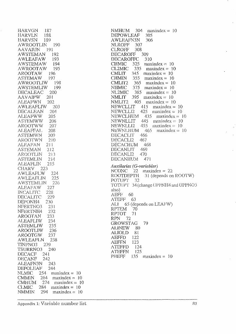
HARVGN 187 HARVLN 188 HARVSN 189 A WROOTLlN 190 AAVAIUN 191 AWSTEMAN 192 AWLEAFAW 193 AWSTEMAW 194 A WROOTA W 195 AROOTAW 196 ASTEMAW 197 AWROOTLlW 198 A WSTEMLlW [99 DECALEAC 200 AAVAIPW 201 ALEAFWN 202 A WLEAFLIW 203 DECALEAN 204 ALEAFWW 205 ASTEMWW 206 AROOTWW 207 ALEAFFAL 208 ASTEMWN 209 AROOTWN 210 ALEAFAN 211 ASTEMAN 2[2 AROOTLIN 213 ASTEMLlN 214 ALEAFLIN 215 CHARV 223 AWLEAFLW 224 A WLEAFLIN 225 A WSTEMLlN 226 ALEAFA \11/ 227 TNCALlTC 228 DECALlTC 229 DEPONH4 230 NFERTN03 23 [ NFERTNH4 232 AROOTAN 233 ALEAFUW 234 ASTEMUW 235 AROOTLlW 236 AROOTGW 237 A WLEAFLN 238 TlNFN03 239 TSURRN03 240 DECACF 241 DECANF 242 ALEAFN3N 243 DEPOLEAF 244 NLMIC 254 maxindex = 10 CMMIN 264 maxindex = 10 CMHOM 274 maxindex = [() CLMIC 284 maxindex = 10 NMMIN 294 maxindex = [()
Appendix 1: Variable number list
NMHOM 304 DEPOWLEAF AWLEAFN3N NLROFF 307 CLROFF 308
maxindex = 10 305 306
DECAROFF 309 DECAROFFC 3 [() CHMIC 325 maxindex = 10 CL2MIC 335 maxindex 0= 10 CMUT 345 maxindex 0= 10 CFIMIN 355 maxindex = 10 CMLIT2 365 maxindex 0= 10 NHMIC 375 maxindex = 10 NL2MIC 385 maxindex = 10 NMLIT 395 maxindex 0= 10 NMLIT2 405 maxindex '" 1 0 NEWCLLlT 415 maxindex = 10 NEWCLLl2 425 maxindcx'" 10 NEWCLHOM 435 maxindex cc 10 NEWNLLIT 445 maxindex = 10 NEWNLLl2 455 maxindex~' 10 NEWNLHUM 465 maxindex = ]() DECACLlT 466 DECACLl2 467 DECACHUM 468 DECANLlT 469 DECANU2 470 DECANHUM 471
Allxilaries (G·variabler) NCONC 22 maxindex·= 22 ROOTDEPTH 31 (depends on ROOTW) POTOPT 32 TUfUPT 34 (changc UPPNH4 and UPPN03 also) AEFF 60 ATEFF 63 ALl 65 (depends on LEAFW) RPTEM 70 RPTOT 71 RPN 72 GROWS TAG 79 ALlNEW 80 ALlOLD 81 AEFFD 122 AEFFN 123 ATEFFD 124 ATEFFN 125 PHEFF 135 maxindex = 10

Appendix 2: 811MVB; Run 80[[.1\1 under the Windows program
The description below rekrs to the program SIMVB.EXE version 1.2 (dated 1996··07··0 I) made by H. Eckcrsten, Sw(,dish University of Agricultural Sciences.
The objectivcs of the SIMVB program are to enable the user of the SOILN model to run the model technically in a simple way, to enable both a strict and flexible presentation of model output, and to enable a simple way of using the model as a tool for evalnation of possible changes in input, calibration, validation and to bring order to input and output files.
Normally, the SOILN model is used together with the SOIL model (Jansson 1991a), therefore the link to SOIL will mentioned below. The SIMVB program is also adapted to the SOIL model and the SPAC model (Eckersten, 1995).
How to run SOJ[LN
RuT!/. under DOS Firstly, we make a short summary of which programs and files that are involved when running SOILN program in an ordinary way under DOS.
The SOlLN model is executed by the program file SOILN.EXE. There arc some associated files to this program. A hclpfilc with variable descriptions etc (SOILN.HLP), a file with standard parameter valucs and othcr informations needed by the model (SOlLN .DEF) and a file including titles and units of the output variables (SOlLN.TRA).
The model is run by using a program file named PREP.EXE. This program helps you to prepare and execute the simulation, i.c. you can select parameter values, input files, simulation period etc. Tbe PI;:EP program describes the ill- and outputs of the model (type for instance, >prcp soiln). All information needed for PREP can be stored in a parameterfile (xxxx.PAR-file). You can give instructions to PREP to read the information directly from the PAR-file. PREP is the program that can activate SOILN.EXE, i.e. to start the simulation. Output from the simulation are stored in two files, SOILNOOl.BIN and SOILNOOl.SUM. The first file (.BIN) includes the values of the simul Hied variables. '1'he second file (.SUM) includes both a summary of all outputs (av(,rages, sums, etc.) alld the prerequisites for the simulation (i.e. the inputs). The file can be Llsed to repeat the simulation if it is renamed to xxxx.PAR.
You can look on the results and make further evaluations of the simulation outputs (SOILNOOl.B1N) witb help of a special program, PG.EXE.
Run. under WINDOWS (SIMVB) The principal iclea for this program (SIMVB.EXE) is to comfortably make use of already developed DOS programs and applications when running SOILN under WINDOWS. The program is restricted to the "administration" of the operative programs and routines. SIMVB.EXE is programmed in Windows-VisualBasic and usecl uncler WINDOWS. The VBRUN300.DLL file should be available.
You start SIMVB from the run option of WINDOWS, or by double clicking the icon (if installed) or by writing under DOS: >win simvb
In the program SIMVB you always start with the heading denoted "Start here". Note, that in the SIMVB program you should always use only single click. First you select model to be used and second the application, which should be stored on disk. Thereafter you normally continue with "Preparation (~lINput". (If you already have macle a complete preparation, and want to have fi'ce access to any part of the program, you select "Check off'. The Check option checks the order in which you select options in the program from preparation to presentation of output during onc run. If you leave the program the Check option is reseted.)
84 SOILN user)s manual

SIMVB enables a good overview of the principal way of using the modc!. If a complete run ("Preparation of INput, Simulation ", etc) has been made, the different options in the schedule can be chosen in any order at any time. However, for the first run, you have to choose them in the following order:
(i) PREPARATION of INPUT. Copies input files to the working directory. Note, that the routines under this option overwrites files at the working directory, without warnings.
(ii) PRESENTATION of INPUT. Variables in input files named AIN_CLIM.BIN, AIN._FERT.BIN etc are presented.
(iii) SIMULATION. The results are stored in files named SOILNCUR.bin and SOILNCUR.sum (CUR denotes the current simulation).
(iv) PRESENTATION of OUTPUT. Variables in SOILNCUR.bin are presented. Variables that are presented are grouped in accordance to subjects like litter N, plant N etc. You can also compare results with the previous run andJor simulations that have heen stored, see below . You can view the summary file of the simulation as well.
(v) STORE FILES. Here you can store the simulation results (SOILNCUR. *) under a different name. You can also recover a previous stored simulation to the name (SOILNCUR. *), thereby making it available for use in the presentation options etc.
(vi) SOIL-SOILN INTERACTION. You should use this option if you want the current SOILN simulation to be input to the SOIL model, or vice versa.
(vii) EXIT the program. You should exit the program by pressing the "EXIT" bottom on the main menu.
Ailternative use of SIMVB
Documentation You can read the SOILN-manual on screen by selecting "Switches etc, Documentation *, Select item, SOILN users manual". In a similar way you can read this SIMVB documentation and the Fortran code of the SOILN model (the model specific code).
'f'ype of User You can select three type of users (Student, Teacher, Research) under "Switches ete ". Different users will get access to different parts of the SIMVB program. Some of the options below is only possible to nse if "Research ON" is chosen.
Give comments By putting the mouse arrow on space between boxes and by making a click on the right bottom you can give comments, on whatever you want. The comments should be stored or cancelled (MAIN MENU) immediately after the option is closed.
Appendix 2: SIMVB; Run SOILN under the Windows program 85

Edit/Hel; You can change a single parameter value or initial state by selecting "Switches etc., Editfiles*" or "Preparation of INput, Changes"', Edit fUes*". Be aware of that you must spell the parameter/variable name correct. As concerns changes in parameter files: Note tbat changes of parameter values preferably are introduced in the AIN_MAN.PAR since values in this file have the highest priority (if you make a change in AIN_PLAN.PAR and the paramcter name also appears in AIN_MAN.PAR the latter is the one used).
Make the simulation under DOS The simulation made by SIMVB can be doue from the DOS prompt as well: demo_vb sim ain_man. In case the SIMVB-program do not start the simulation properly, you can use this command to make the simulation and then go back to SIMVB for presentation of output.
Use PREP·program manuaUy The PREP-program can be run in a standard (interactive) way within SIMVB. If you have made "Preparation !d'INput, Normal* .... " the prepared AIN._xxxx.PAR files arc read by PREP. The files are read in the following order: AIN_SOIL.PAR, AIN....PLAN.PAI<, AIN_.OUT.PAR, AIN_TIME.PAR, AIN_MAN.PAR. Simulation results are stored in SOILNcllLBlN as in the normal simulation.
If you do not want to load the parameters files you have chosen with preparation, then select "Switches etc, Check !d!" before entering PREP. Note that output file now is named SOILNxxx.BIN (where xxx is a number between 001 and 999) and if you want to make use of presentation of output options it has to be restored to SOILNcur.BIN (use "Storefiles*, xxx to Current").
Use PG"program mnnuaUy The PG program can be used in a standard (interactive) way within SIMVB. Select "Switches etc, PG ON".
Uge iExcel·progrnm. maffwudly The Excel-program can be used in a interactive way within SIMVB, in case Excel is loaded and there is a path to Excel. Select "Switches etc, Excel ON". SIMVB converts the PG·binary-file concerned to db!' or lotus 123 format and brings you automatically into Excel. With help of the presentation routines of SIMVB you can select variables to be exported to Excel.
Print files Graphs plotted on screen can also be stored on TEK-files. Select "Switches etc, Plot Tekfiles, Make Tek~files". The files can be printed on screen or paper, or converted to metafilcs (.CGM-file) that can be imported to documents and graphical programs ("Switchesetc, Print/tles*" .... ). Under this option also ASCII files can be printed.
UI;ing only one parameter file To run SIMVB with only one parameter file, there arc two possibilities:
(l) Really, using only one parameter file: In this case the simulation is completely governed with it single parameter. Store the file under name AIN_ ONE.P AR and select "Switches etc, onc par~tile".
86 SOILN user's rnanual

(2) Actually, using two parameter files: In this case you make use of the parameter file AIN_OUT.PAR selecting proper outputs for the SIMVB presentation routines. The content of the other four parameter files are put together into the AIN_MAN.PAR file. Note that you should take away (i) the declaration of file names except for FILE(9), which should be named AIN_FERT.BIN if it is used, and (ii) the OUTFORN switch. The three other parameter files have to exist but should be empty except for a";" (AIN_.OUT.PAR is delivered by SIMVB automatically).
Making the five parameter fUes Under the option "Preparation oj'INputs, normal"''' the five parameter files AIN_SOIL.PAR, AIN]LAN.PAR, AIN_OUT.PAR, AIN .. TlME.PAR and AIN_MAN.PAR can be created automatically from the last simulation (i.e. from SOILNcULSUM·file).
Multiple rum; Up to 6 multiple simulations can be done and plotted. (It is the presentation of output that limits the number of simulations.) ("Preparation of 'INput, Multiple simulation, Simulation, Others"', Multiple simulation, Presentaion ot'OUTput*, Multiple simulation")
Initial states ofplI"eviorus run. Make a simulation using outputs of the previous simulation as initial states in the new simulation. ("Simulation, Others*, Initial values ... ")
FUe list In the "Preparation of INput, Normal* ... " option of SIMVB files can be selected arbitrary by selecting ':file list*" in the list menus. This is a compliment to the other preparation options.
AUenrudilJe appUcaU«ms wuler directory", \XXXXL, Often several versions of the same main application is wanted to be run by STMVR For the "Standard" application one way of storing them separately and to be able to run them under SIMVB is to do as follows: 1) Store the main application with a full set up of input files under ... \XXXX\N\NA, as usual. 2) Stow the files chauged due the specific version under a separate directory named fi. VERSION I, i.e .... \NA \VERSION 1. Do not changc the name of the files and remember to store the INFO.US file in which you give an identification of the application stored in the directory. 3) Copy files from VERSIONI directory to working directOlY by selecting "Preparation (~t' INput, normal"', Prep. from SubDir, Directory, Preparation"
Change instruction files The instruction files used by the PG· program are stored under the directory C:\SIMVB\xxxxx\N\NA\PG. If you want the drawing to be made in another way or other variables to be selected you can edit these. The address to the file to be edit you get by selecting "Switches etc, File name" immediately after making a plot or any other operation (this option is not available for all files).
Adaptation of application to SIMVB The description below refers to a "Standard" application.
Appendix 2: SIMVB; Run SOILN under the Windows program 87

SOILN If you would like to run the SOILN model under the SIMVB program, there are principally two different starting points. Either you have an own application already working under DOS or you have not yet parameterised SOILN for your site. Below will be described one procedure to follow in the latter case. In the former case, see the bottom of this section.
I) Install the SIM_96 application used for the simulation course on SOIL-SOILN held at SLU in Mars 1996. The application refers to the Kjettslinge site north of Uppsala (Andren et a1. 1990) can be delivered by Henrik Eckersten or Thomas Katterer ([email protected]) at SLU.
2) Check that the application works in its original version, on your computer.
3) Replace the files denoted AIN_ .... under C:\SIMVB\N\NA\KJETTSL-direclory to those of your application. In INFO.LIS file you write the information that it is your directory now.
-a) Start by replacing AIN_.CLIM.BIN (the driving variable file taken from the SOIL model) to that of yours. -b) Change in AIN_SOIL.PAR the number of soil layers (NUMLA Y) and the thickness oflayers (THICK) -c) Change in AIR.TIME.PAR the time period to be simulated. -d) Ruu SIMVB and check tbat a simulation is done and that you receive results.
-e) Replace AIN_SOIP.DAT (soilp.dat-file) with yours. of) Change in AIN_SOIL.PAR the identification of your profile (UNUM, UPROF) -g) Run SIMVB and check that a simulation is done and that yon receive results.
-h) Change other parameters in the parameter files in accordance with your application -g) Run SIMVB and check that a simulation is done and that you receive results.
4) Rename your application to standard format: After the two first points above your application set is technically ready, however, named SIM_96\S\SA\KJETTSL. Your results will not be affected by this. If you, however, want to put your application under standard format with a proper name (for instance Mellby) you do it this way:
-a) Create a directory C:\SIMVB\MELLBY\N\NA b) Copy the content of C:\SIlV1VB\SIM_.96\N\NA\KJETTSL la that directory
-c) Create the following directories: C:\SIMVB\MELLB y\N\NA \PG C:\SIMVB\MELLBY\N\NA\START
-d) Copy the content of the corrcsponding directories for SIM_96 to those directories
5) Start SIMVB, choose SOILN model, Standard. Write MELLBY. Make preparation ("Preparation of INput, Initial, Normal*, Full preparation ") and simulation ("Simulation, Normal") and presentation of output "Presentation of OV7Jmt* ... ".
Additional information: The description above does not handle the conversion of AIN_BOUN.BIN and MEAS.BIN. Those files are not necessarily needed. AIN_BOUN.BIN is needed if you choose the BOUNDARY-switch> 0, see manual above. MEAS.BIN is used for comparison between simulated and measured data ("Presentation of OUTput*, Validation"). You can not convert these two files straight forward to your application since you probably have measured other variables at other time points. However, you can use the principal structure of the files. As concerns MEAS.BIN you have to change in the PG-instruction files making the comparison. If you choose "Switches etc, File name" you get the address of the file used for the presentation. Replace that file(s) with the one(s) you want to apply for the comparison.
There are 4 parameter files. However, you do not necessarily need to have more than one, see the section above on Alternative use of SIMVB, using one parameter file together with an output parameter file. In case you already have an application working under DOS, you should follow the same procedure as above, except that you, in this way, replace the Kjettslinge parameter files with yours.
88 SOILN user's mannal
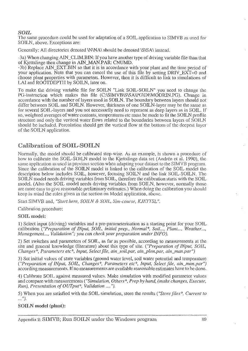
SOIL The same procedure could be used for adaptation of a SOIL application to SIMVB as nsed for SOILN, above. Exceptions are:
Generally: All directories denoted \N\NA\ should be denoted \S\SA\ instead.
-3a) When changing AIN_CLIM.BlN: If you have another type of driving variable file than that of Kjettslinge then change in AIN_MAN.PAR: CNUMD. -3b) Replace AIN_EXT.B1N so that it is in accordance with your plant and the time period of your application. Note that you can cancel the use of this file by setting DRlV _EXT=O and choose plant properties with pm·ameters. However, then it is difflcnlt to link to simulations of LAl and ROOTDEPTH by SOILN, later on.
To make the driving variable file for SOILN "Link SOIL-SOILN" you need to change the PG-instruction which makes this file (C:\SIMVB\S\SA\PG\DEMODRIN.PG). Change in accordance with the nnmher oflayers nscd in SOILN. The boundary between layers should not differ between SOIL and SOILN. However, thickness of one SOILN.-Iayer may be the same as for several SOIL-layers and you not necessarily need to represent as deep layers as in SOIL. If so, weighted averages of water contents, temperatures etc must be made to fit the SOILN profile structure and only the vertical water flows related to the boundaries between layers of SOILN should he included. Percolation should get the vertical flow at the bottom of the deepest layer of the SOILN application.
Calibration of SOIL-SOILN Normally, the model should be calibrated step-wise. As an example, is shown a procedure of how to calibrate the SOIL-SOlLN model to the Kjettslinge data set (Andren et al. 1990), the sallle application as used in previous section when adapting your dataset to the SIMVB program, Since the calibration of the SOILN model is linked to the calibration of the SOIL model the description below includes SOIL, however, focusing SOILN and the link SOlL-SOILN. The SOILN model needs driving variables from SOIL, therefore the calibration starts with the SOIL model. (Also the SOIL model needs driving vm-iables from SOILN, however, uormally those arc more easy to give reasonable preliminary estimates.) When doing the calibration you should keep in mind the rules given in the section on Model application, above.
Start SIMVB and, "Start here, SOlLN & SOIL, Sim-course, KJEI1~r:;L".
Calibratiou procedure:
SOIL model:
1) Select input (driving) variables and a pre-parameterisation as a starting point for your SOIL calibration ("Preparation of INput, SOIL, initial prep., Normal"', Soil ... , Plant ... , Weather ... , Management ... , Validation "; you can check your preparation under INFO).
2) Set switches and parameters of SOIL, as far as possible, according to measurements at the site and general knowledge (literature) about this type of site. ("Preparation of INput, SOIL, Changes"', Parameters etc*, Input, Selectfile, ainj·oil.par, ain .. plan.par, ain_man.par")
3) Set initial values of state variables (ground water level, soil water potential and temperature ("Preparation q/INput, SOIL, Changes"', Parameters etc"', Input, Select file, ain_man.par") according measurements. If no measurements are available reasonable estimates have to be done.
4) Calibrate SOIL against measured values. Make simulation with modified parameter values and compare with measurements ("Simulation, Others"', Prep by hand, (make changes, Execute, Run), Presentation of o UT put *, Validation .... ").
5) When you arc satisfied with the SOIL simulation, store the results ("Storefiles"', Current to ... 11),
SOILN model (plant):
Appendix 2: SIMVB; Run SOILN under the Windows program 89

6) Set switchcs and parameters of SOILN-vlant, as far as possihle, according to measurements at the site and general knowledge (literature) about this type of plant. ("Preparation of/Nput, SOILN, Changes"', Parameters etc*, Input, Seleclfile, ain-lJlan.par")
7) Select input (driving) variables and a prc-parameterisation as a starting point for your SOILN calibration ("Preparation of INput, SOILN, initial prep., Normal*, Soil ... , Plant ... , Weather ... , Management ... , Validation").
8) Extract the driviug variables of SOILN from your SOIL simulation ("Link SOIL-SOILN*, SOIL to .... ").
9) Set initial values of plant state variables ("PreparationofINput, SOILN, Changes*, Parameters elc*, Input, Seleetfile, ain_.inLini")
I 0) Calibrate the plant N uptake process. Since plant N uptake usually is the largest N flow in the system, an appropriate calibration of this process is especially important. You should be aware of not introducing errors due to problems in simulating N availability in soil. That problem you intend to solve later. So you should use the measured values of soil mineral N, instead of the simulated N, as the source for N uptake. You do this by choosing "Auto correction" of both N03 and NH4 values ("Preparation of INput, SOILN, Normal*, Management (Both NH4 and N03 correction),,) (see BOUNDARY-switch).
The N uptake process coule! be separated into three different processes that we suggest that you consider in the following order. a) The growth of plant is determining the potential demand for N. You calibrate this process against measurements on total above ground plant biomass. b) The actual N uptake is then calibrated against measurements on total above ground plant N. This is done by the maximum N levels of the different tissues, which determines the ultimate demand, and the possibility to extract N from the mineral N pool. e) 'rhc phenology or/and allocation to grain you calibrate against measurements on grain biornass and N. Note, that a), b) and c) arc inter dependent and that a correction under b) might lead to that you have to modify the calibration under a). 'fhe calibrations you do by making simulation with modified parameter values and compare with measurements ("Sinuliation, Others'", Prep by hand, (make changes, Execute, Run), Presentation !fOUTput*, Validation .... "}. Note that the "Prep by hand" statement do not store the modified parameter selling in your parameter files, i.e. next time you start from the original parameter setting.
11) When you arc satisfied with the SOILN plant simulation, store the results ("Store .tiles*, Current to ... ").
12) Introduce the new parameter setting into the parameter files. ("Preparation rfINput, SOlLN, Changes*, Parameters etc*, Input, Select .tUe, ain_.\·oil.par, ain-lJlan.par"). Note if you have made changes of parameters in ain_man. par you have to introduce these changes into ain_.man.par each time after you have made a management preparation.
SOKLN model (soil):
13) Set switches and parameters of SOILN-soil, as far as possible, according to measurements at the site and general knowledge (literature) about this type of site. ("Preparation (!f INput, SOILN, Changes*, Parameters etc*, Input, Select file, ain_.\·oil.par")
14) Calibrate the soil N processes against measured values on ammonium N anclnitrate N. We suggest the following order for calibration: a) First calibrate the nitrification and denitrification processes to fit the measured values of nitrate. You should use the measured values of ammonium instead of the simulated values ("Preparation of INput, SOILN, Normal'", Management (NH4 AutoCorrect),,). b) Calibrate the mineralisation process to fit the measured values of ammonium. You should use the measured values of ammonium instead of the simulated values ("Preparation «I' INput, SOILN, Normal*, Management (N03 AutoCorreet),,).
90 SOILN user's lTWl1ua]

The calibrations you do by making simulation with modified parameter values and compare with measurements ("Simulation, Other~\'*, Prep by hand, (make changes, EKecute, Run), Presentation (,/OUT/JUt*, Validation .... ").
15) When you are satisfied with the SOILN simulation, store the results ("Store.files*, Current to ... ").
16) Take away the auto corrections ("Preparation (,f INput, SOlLN, Normal*, Management (Fertilis (Rl20)),,).
17) Introduce the new parameter setting into the parameter files. ("Preparation oj'fNpUi, SOILN, Changes", Parameters etc*, Input, Select file, ain. __ soil.par, ail1-1Jlan.par")
18) Make a simulation, without auto corrections, and regressions hetween simulated and measured values, of all variables (plant biomass, plant N and so on ... ) ("Simulation, Normal, (make changes, Execute, Run), Presentation of OUTput", Validation .... ").
illteractiolls:
19) Note, there is an iuter dependency between 10) and 14) which might require changcs of the plant N uptake calibration. YOll might have to do 10 .. 12) and 1418) again.
20) When you are Batisfied with the SOILN simulation, store the results ("Storeflles*, Current to ... ").
21) Extract leaf area index and root depth to be used as inputs for a new SOIL simulation ("Link SOlL-SOlLN*, .... to SOIL").
22) Since the leaf area and root depth as simulated by SOILN probably differ from those used in the previous SOIL simulation you have to do the calibration procedure points 4 .. ,5),8), 10 .. 12) and 14-21) again.
File description of SIMVB The description below refers to a "Standard" application.
Dire<r:tmy strnuciuF'e The directory name given when choosing an application should be XXXX in: c:\sim\soilns\XXXX (c:\sim\soilns\ cau be another address, if you specify it under "Switches etc." just after selected "Start here").
Uncler the application directory we find the "WORKING .. directory" named ... \XXXX\N. In the "working-directory" all your preparations and simulation res nits arc stored. The meaning is that it is up to the user to delete files within the directOlY. Original files can always be recovered from directories below this one. First time you run the program the directory is empty. When you run the program and make preparation, files are stored on the "working-direetory". SIMVB writes files only on this directory (except for comment.txt under the application directory). (For the SOIL model the "working-directory" is named ... \XXXX\S.)
ln the STORE-directory ( ... \XXXX\N\NA) below the "working-directory" program and data files are stored. Files in this directory as well as below this directory should not be deleted by the user.
Firstly an "initial preparation" is made. Then files arc copied from ... \XXXX\N\NA\START. These are files related to programs and are common for all applications.
PG-instruction files used for presentations etc. are stored in ... \XXXX\N\N A \PG. Files are copied from this directory to the "working directory" as soon as PG is liBel!. Some files are stored at the "working directory" to allow the user to make changes in the presentations. They are not overwritten until a new initial preparation is made.
Appendix 2: SIMVB; Run SOILN uncler the Windows progrmn 9l

When selecting an option within the "Preparation" option files arc copied from the store directory ... \XXXX\N\NA. These are input files but also validation files for a certain application. Application information is given in the INFO.LIS file.
Other "sub-applications" can be stored below the store directory ( ... \XXXX\N\NAJ. Those applications can be stored on the "working directory" making use of the "preparation from sub-directories". Only the changes compare to the application stored under ... \XXXX\N\NA is needed to be given here.
Files Directory ... \XXXX; "Application directory" COMMENT LIS Comments given by the user while running SIMVB. Directory ... \XXXX\N; "Working directory" AIl\l_.CLIM BIN Driving variables ''AIN_CLIM BPR AIN._CLIM.BIN used in previous run "'AIN_FERT BIN N input variables 'AIN]ERT BPR "AIN_FERT DAT ""AIN_F'E:RT DDE AIN . .INI 1Nl AIN_MAN PAR
AIN .. _SOIL PAR
AIN_SOIP DAT AIN_TIME PAR DEMO_.COP BN],
DEMO.VBBAT "DEMOCOMX PG MDEMOPCAR PG
"'DEMOPCOM PG
"'DEMOPNIT PG
'DEMOZVAL BIN INFO LIS "'MEASBIN
"SOILN FIN 'SOILN STA SOILN THA 'SOILNCUR BIN 'SOILNCUR SUM 'SOILNPRE BIN
92
Version of AIN_FERT.BIN used in previous run N input variables as ASCII Variable description for AIN_.FERT.DAT Initial values of state variables Management parameters. Parameter Groups and Switches denoted (M) and file speciflcation for files related to management (FILE(9) form SOILN). (Read by PREP as nr 5) Output variables. Parameter Groups and Switches denoted (0) and file speeifieations not related to management. Note, that OUTFORN must be ON otherwise none of the PG-instruction filos will work, f.i. The "PRESENTATION" options. (Head by PREP as nr 3) Plant parameters. Parameter Groups and Switches denoted (P). (Read by PREP as nr 2) Soil parameters. All Parameter Groups and Switches denoted (S) or not found elsewhere. (Read by PREP as nr 1) Soil physical data (from PLO'l'PF'.l<;XE) Simulation period. (Read by PREP as Hr 4) Program flle that copies flles from different directories to the working directory. Program flle. Bat-file used to make simulations ete, PG-instruction me PG-instruction flle in which variables for plotting can be selected ("Presentation of OUTput, Carbon, Other'~ PG-instruction flle in which variables for comparison can be selected ("Presentation of OUTput, Comparison, .. " Other'~ PG-instruction flle in which variables for plotting can be selected ("Presentation of OUTput, Nitrogen, Other") Presentation data Information about the application loaded on the working directory Values to be compared with the simulation outputs ("Presentation of o UTI' ut, Validation'~ Output state variables in a form possible to be used as input A counter used by SOILN Data description for Output variables Output variables from the current simulation Data description for the bin··me Output variables from the previous simulation
SOILN URCeS 111anual
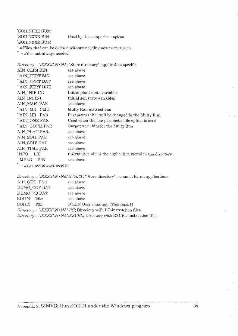
"SOILNPRE SUM "SOILNXXX BIN
'SOILNXXX SUM Used by the comparison option
" = Files that can be deleted without needing new prcparation " = Files not always needed
Directory ... IXXXXININA; "Store directory", application specific AIN_CLIM BIN sce above MAIN_FERT BIN see above "AIN._FER1' DAT sce above "AIN_FERT DDE
AIN . .INIP 1Nl AIN._INI INI AIN._MAN PAR "AIN_MR CM!)
"AIN_MR PAR "AIN_ONE PAR "AIN_OUTM PAR
AIR.PLAN PAR AIN._SOIL PAR AIN_SOII' DAT
AIN:rIME PAR INl'O LIS
see above Initial plant state variables Initial soil state variables see above Multy Run instructions Parameters that will be changed in the Multy Run Used when the ono-parameter file option is used Output variables f,)r the Multy Run see above see above BCG above soo above Information about the application stored in the directory
'<'MgAS BIN see above
." ::::: li'iles not always needed
Directory ... IXXXXININAISTART; "Store directory", common for all applications AINJHJT PAR see above
DEMO .... COP BAT DEMO.YBBAT SOILN 'l'RA
see above sco above see above
SOILN 'l'XT SOILN User's manual (This report)
DirectOl:Y ... IXXXXININA IPG; Directory with PG .. instruction Illes Di/'ecto/)' ... IXXXXININA 1 EXCEL; Directory with EXCEL-instruction files
Appendix 2: SIMVB; Run SOILN undor the Windows program

j
j
j
j
j
j
j
j
j
j
j
j
j
j
j
j
j
j
j
j
j
j
j
j
j
j
j
j
j
j
j
j
j
j
j

F6rteckning ovcr lltgivna hliftCll i pllblikalionsscricn
SVERIGES LANTBRUKSUNIVERSITET, UPPSALA. INSTITUTIONEN FOR MARKVEfENSKAP. AVDELNINGEN FOR LANTBRUKETS HYDROTEKNIK. A VDELNINGSMEDDELANDE. 1'1' 0 111 1993
93: 1 Jansson, C. Rckonslruktion av naturlig vallenWring i Ostcrdalalvcn oeh vkirdcring av rcglcringsnytta. 30 s + 5 bi!.
93:2 Linner, H., Pcrsson, R, Bcrglund, K. & Karlsson, S.~E. Resultat av 1992 ai'S rHltfCirs()k avsccnde detaljavvattning, markvard oeh markft)rbtiHring saml bevattning. 83 s.
93:3 Jod, A. & Wcsstri)m, 1. Vattcnilushfillning yid bcvaltning ~ en sludie av lilJHmpad bevattningstreknik i Sidi Bouzid~distriklct, Tunisien. 54 s.
93:4 Jansson, P~E. SOIL mOdel. User's Manual. Second edition. 65 s.
93:5 Danfors, B. & Linncr, H. Resursbevarande odling med markUickning oeh gnmd inbrukning av viixtma(erial. fl6 s.
93:6 Jansson, P~E. PLOTPF. User's manual. 33 s.
93:'7 Bath, A. Studier av rotlJtveckiing och markvattenhalt i Hirsiik mcd marklHckning. 71 s.
94.: J Tabcll, L. 'I:Hile i torvjord. 46 s
94:2 Halldorr, S. RUlloff water as a soil forming facto!' in arid zones. 62 s.
94:3 Jansson, P~E. SOIL model. User's Manual. Third edition. 66 s.
94:4 Eekc!'stcn, Hq Janssoll, P~E. & Johnssol), i-I. SOILN model. User's manual. Second edition. S8 I).
94:5 Pcrsson, R. (cd.). Proceedings, NJF~scl11inar no 247, Agrohydrology and nutrienl balances, Oclober J 8~20, 1994, UppsaJa, Sweden. J 11 s.
95: 1 Alnvi, G. Radial stem growlh IInd trampirlHion of Norway spruce in relation 10 soii waleI' availability. Granens tillvUxt oeh transpiration i relation till markvattnets (i!lg;inglighet (Licenciat(lvhandling). 13 + 11 + 14 s.
95:2 Johansso!1, W. & Fellin, O. Biogas fdlll vall. Tcknik (Jcll ekollorni vid o(\ling, skiird, transporter, ensilering samt rOlning 1l1ed tviistegslcknik. 38 s.
95:3 Svensson, E., Llnncr, l-I. & Carlsson, H. UtvHrdering av viixtanalys j blbrikspotatis, 53 s.
95:4 Andcrsson, A. VaHentillgangar fOr bcvaltning i Kalmar Hin.I. Lilteratur(iversikl.ll.lntcrvjuundersi.ikning ri)randc vattcnmagasin. 48 s.
95:5 Wesstrd))1, I. Bcstiimning av markens salthalt genom mlitning mcd konduktivitctssOlld. 18 s.
95:6 Eckerstcn, IL, Janssoll, P~E., Karlsson, S., Perssol1, B., PerUu, K. & Ancicrsson, 1. En inlroJuktion till biogc"ofysik. 72 s.
95:7 Eckersten, H. Simulation of water now in pJant communities. SPAC model description, exercises and user's manual. 49 s.
95:8 Nabician, F. Simulcring av vattenbalans f()r energiskog Pll en lorvmark. 25 s.
96:1 Eckerstcn, H., J,l!lsson, P-E., & Johnsson, 11 SOILN model, user's manual. Version 9.1. 93 s.

j
j
j
j
j
j
j
. j
j
j
j
j
j
j
j
j
j
j