Sustainable Development and Industrial Development ... · PDF file1 Sustainable Development and Industrial Development: Manufacturing Environmental Performance, Technology and Consumption/Production

by

Marianna Gilli, Giovanni Marin, Massimiliano Mazzanti, Francesco Nicolli

Sustainable Development and Industrial Development: Manufacturing Environmental Performance, Technology and Consumption/Production Perspectives

SEEDS is an interuniversity research centre. It develops research and higher education projects in the fields of ecological and environmental economics, with a special focus on the role of policy and innovation. Main fields of action are environmental policy, economics of innovation, energy economics and policy, economic evaluation by stated preference techniques, waste management and policy, climate change and development.

The SEEDS Working Paper Series are indexed in RePEc and Google Scholar. Papers can be downloaded free of charge from the following websites: http://www.sustainability-seeds.org/. Enquiries:[email protected]

SEEDS Working Paper 01/2016 March 2016 by Marianna Gilli, Giovanni Marin, Massimiliano Mazzanti, Francesco Nicolli

The opinions expressed in this working paper do not necessarily reflect the position of SEEDS as a whole.

http://www.sustainability-seeds.org/

mailto:[email protected]

1

Sustainable Development and Industrial Development:

Manufacturing Environmental Performance, Technology

and Consumption/Production Perspectives*

Marianna Gilli† Giovanni Marin

‡ Massimiliano Mazzanti

§ Francesco Nicolli

**

Abstract

Industrial development has always been seen as the main engine for economic

growth due to its large economic multiplier and technological opportunities.

However, manufacturing sectors are directly and indirectly responsible for a large

share of overall environmental pressures, raising concerns for the environmental

sustainability of manufacturing-based development. In this paper we evaluate the

drivers and decoupling trends of environmental pressures arising (directly or

indirectly) from manufacturing production and consumption for a large selection

of developed and developing countries.

As a first step we decompose changes in emission intensity of manufacturing

sectors into a series of components by means of a shift-share analysis to identify

the main drivers of change. A second step will compare direct environmental

pressures generated by manufacturing sectors (production perspective) with the

amount of emissions generated (domestically and abroad) by the domestic

consumption of manufacturing goods (production perspective). Finally, we

evaluate the possible emergence of an EKC dynamics for production and

consumption perspective emissions for the world as a whole and for different

continents.

Keywords: industrial development, environmental efficiency, shift share analysis,

production-consumption perspective, environmental Kuznets curve

JEL: Q55, Q56, O19

* Massimiliano Mazzanti acknowledge financial support from the UNIDO. We thank Nicola Cantore (UNIDO) for very

helpful comments. Usual disclaimer applies. † University of Ferrara & SEEDS (Italy), e-mail: [email protected]

‡ IRCrES-CNR & SEEDS (Italy), e-mail: [email protected]

§ University of Ferrara & SEEDS (Italy), e-mail: [email protected]

** IRCrES-CNR & SEEDS (Italy), e-mail: [email protected]

2

1 Introduction

This work aims at analysing the environmental performances of manufacturing sectors and their

main drivers, namely economic factors, technology and trade among others. In particular we focus

here on the dynamic development of environmental performances, both in absolute terms and in

‘productivity’ terms, through both decomposition and an econometric analyses. The analysis aims

to highlight differences over time, across geographical areas, income categories and by sectorial

technological classes. Strong emphasis is assigned to the comparison of consumption and

production perspectives1, while the main framework of reference is based on the Environmental

Kuznets curve (EKC) approach. This paradigm allows investigating how environmental

performances are (dynamically) affected by population (Martinez-Zarzoso et al. 2007), GDP,

technology (Vollebergh & Kemfert 2005), composition effects and trade (see in particular Levinson

2009, for a discussion of the role of trade, composition and technology as drivers of a country

environmental performance).

Before delving in more detailed discussions on sectoral performances, it may worth taking a step

back to the aggregate environmental-income relationship. Recent studies on the dynamics of CO2

by country outline that high income countries have slightly reduced their direct emissions in

manufacturing sectors overall (Musolesi et al. 2010), while both medium low and medium high

income groups have witnessed increases. The depicted situation clearly shows that there is still an

increasing production of carbon dioxide worldwide. It is worth noting that there could be a ‘link’

between the higher elasticity of carbon dioxide to income in medium low and medium high income

groups and the role of trade (e.g. moving production abroad, off-shoring and out-sourcing

production of heavy manufacturing as key examples), which explains part of the emission reduction

in high income countries. Worldwide emissions in manufacturing sectors are somewhat increased

due to the process of deindustrialization/demanufacturing of more advanced countries and to the

fact that goods are produced with higher CO2/value added intensity in emerging countries. Being

such demanufacturing a natural evolution of economic systems (Baumol 1967; Rodrik 2013),

environmental and innovation policies should favour technological transfers, in addition to the aim

of minimising the costs of complying with environmental regulations in the short run, when the two

aspects may be in conflict. Finally, technological change is another piece of this complex puzzle, as

high technological intensity and high value added specialization allow reducing emissions, then

1 Following EEA (2014) the production perspective approach considers only direct domestic emissions while final

demand consists of total final demand (domestic demand and export) of domestically produced goods. The consumption

perspective approach considers also foreign emissions by including in the matrix of inter-industry transactions both

domestically produced and imported intermediate inputs, while final demand includes overall demand by resident

agents, thus including domestic and imported final consumption but excluding exports.

3

trade development (e.g. increased net imports of polluting goods) may further contribute to this

reduction2, making necessary to explore both production and consumption perspectives (Marin et

al. 2012; EEA 2014a) along the evolution of economic systems. It is worth noting the joint role of

economic value and technology to generate emission reductions: those are two factors that are

characterised by dynamic co-causations, one being the driver of the other and vice versa (Costantini

& Mazzanti 2012; Costantini et al. 2013). Nevertheless, only a robust technological progress may

reverse the CO2 increasing trend. These empirical facts shortly but coherently narrate pieces of a

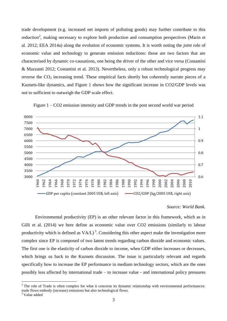
Kuznets-like dynamics, and Figure 1 shows how the significant increase in CO2/GDP levels was

not to sufficient to outweigh the GDP scale effect.

Figure 1 – CO2 emission intensity and GDP trends in the post second world war period

Source: World Bank.

Environmental productivity (EP) is an other relevant factor in this framework, which as in

Gilli et al. (2014) we here define as economic value over CO2 emissions (similarly to labour

productivity which is defined as VA/L) 3

. Considering this other aspect make the investigation more

complex since EP is composed of two latent trends regarding carbon dioxide and economic values.

The first one is the elasticity of carbon dioxide to income, when GDP either increases or decreases,

which brings us back to the Kuznets discussion. The issue is particularly relevant and regards

specifically how to increase the EP performance in medium technology sectors, which are the ones

possibly less affected by international trade – to increase value - and international policy pressures

2 The role of Trade is often complex for what it concerns its dynamic relationship with environmental performances:

trade flows embody (increase) emissions but also technological flows. 3 Value added

0.6

0.7

0.8

0.9

1

1.1

3000

3500

4000

4500

5000

5500

6000

6500

7000

7500

8000

19

60

19

62

19

64

19

66

19

68

19

70

19

72

19

74

19

76

19

78

19

80

19

82

19

84

19

86

19

88

19

90

19

92

19

94

19

96

19

98

20

00

20

02

20

04

20

06

20

08

20

10

GDP per capita (constant 2005 US$, left axis) CO2/GDP (kg/2005 US$, right axis)

4

to reduce emissions. The second aspect refer again to the role of technological progress, which can

be seen as the main element capable of influencing this elasticity, allowing in other terms to sustain

a certain level of living standard reducing the impact to the environment. On this point, Vollebergh

and Kemfert (2005) observe for instance that for Carbon dioxide emissions decoupling is not yet

apparent and that radical changes in energy technologies are essential. They conclude that: ‘directed

technological change conveys a positive message i.e., that shifting away from polluting

technologies towards non- or less polluting technologies seems both possible and manageable

through environmental policy (...). A widespread belief seems to exist that environmentally induced

technological change would yield a double dividend’ (p. 144). Technology and time-related effects

deserve careful attention.

Trade issues will be carefully scrutinised in our paper, namely by considering the role of trade

openness and ‘production vs consumption’ perspectives (e.g. increased net imports of polluting

goods) to explain dynamic environmental performances by countries and world areas. The core

hypothesis that regards trade and country emission performances revolves around a couple of

critical points. On the one hand the pollution haven hypothesis (Keller & Levinson 2002) suggests

that more stringent environmental regulations in high income countries move emission intense

production abroad; on the other hand we should be aware that environmental regulations costs are

only a fraction of total costs and, in addition, rich countries could still have price unrelated (non-

Ricardian) competitive advantages (motivated by the Heckscher Ohlin theorem), which relate to the

abundance of (emissions heavy) capital (Wagner & Timmins 2008). Empirical evidence should

provide guidance and shed light on the role of trade. Levinson (2009) concludes for the US: ‘For

the typical pollutant, increased international trade explains less than one-third of the pollution

reductions from composition changes in US manufacturing, and only one-tenth of the overall

pollution reductions from manufacturing. By far the most important contributor to reducing

manufacturing pollution has been technology’. We here focus on carbon dioxide emissions and not

pollutants as such. The evidence on the role of technology, income and trade is geographically and

time specific. In the following, we offer a macroeconomic glance with a focus on main world areas.

The following sections convey new evidence on the income, trade and technology drivers of carbon

dioxide emissions produced by industrial development. We will present insights based on

econometric and decomposition analyses, which touch both the production and consumption side of

environmental performances. Section two decomposes manufacturing CO2 emission performances

across countries through a shift-share analysis. Section three discusses the so called consumption

and production perspective, and introduces the main data used in the analysis. Section four presents

5

empirical exercises aimed at testing for the presence of a non-linear EKC path, accounting for the

role of technological change. Finally, Section five lists the main highlights and original outcomes.

2 Decomposition analysis of emissions in the manufacturing sector

In this section, we present a decomposition analysis which relies on the geographical dimension

only (shift share analysis), by comparing each country with the world-average and the geographical

and income-class average. In doing that we exploited two different data sets. The Real value added

in US dollars by manufacturing sectors (ISIC Rev 3.1) comes from the INDSTAT2 database

maintained by the UNIDO, while CO2 air emissions from the combustion of fossil fuels are

retrieved from the corresponding database maintained by the International Energy Agency (IEA)4.

Shift share analysis is a common tool in regional and urban economics (e.g., Esteban 2000): its aim

is to quantify the role played by different factors in driving growth or intensity differentials between

a single region (or a single country) and a benchmark (for instance the country in which the region

is contained or, in our case, the countries with respect to the world average). Concisely, the

technique decomposes the differential in the variable of interest between each regional and the

national average into its two main factors: the region performing generally better than average or a

regional specialisation in fast growing sectors. In the present paragraph, we adopt the shift-share

analysis to decompose the total emission efficiency (emissions per value added) differentials for the

manufacturing sector into three components, called structural (M), differential (P) and allocative

(A), which can be interpreted as follows5:

1. The differential factor (P), which reflects that part of the difference in emission intensity of a

country is due to differences in within-industry environmental efficiency. The index assumes

positive (negative) values when the country is less (more) efficient in term of emissions, under

the assumption that the country sectoral composition is the same.

2. The structural factor (M) reflects a country sectorial mix, and quantifies the contribution of

differences in the composition of the manufacturing sector to aggregate differences in emission

efficiency. This value assumes positive (negative) value if the region is specialised in more

(less) emission-intensive sectors (according to the chosen indicator).

3. Finally, the last factor, called allocative component (A) is calculated as the covariance between

the previous two components, and represents the contribution to the emission differential

between the country and the world average given by its specialisation in more environmental

4 See Appendix A for more details on data sources.

5 In doing so we follow Gilli et al. (2013) to which we refer for further details on this approach. Moreover, Appendix B

present a mathematical appendix with the derivations of the M, P and A terms.

6

efficient sectors. A positive (negative) value would mean that country is specialised in more

(less) polluting sectors, which are less (more) efficient with respect to the world average.

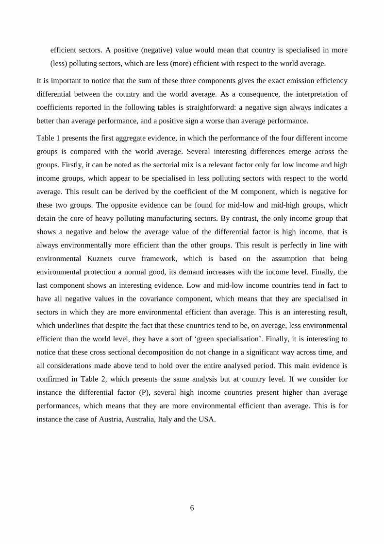
It is important to notice that the sum of these three components gives the exact emission efficiency

differential between the country and the world average. As a consequence, the interpretation of

coefficients reported in the following tables is straightforward: a negative sign always indicates a

better than average performance, and a positive sign a worse than average performance.

Table 1 presents the first aggregate evidence, in which the performance of the four different income

groups is compared with the world average. Several interesting differences emerge across the

groups. Firstly, it can be noted as the sectorial mix is a relevant factor only for low income and high

income groups, which appear to be specialised in less polluting sectors with respect to the world

average. This result can be derived by the coefficient of the M component, which is negative for

these two groups. The opposite evidence can be found for mid-low and mid-high groups, which

detain the core of heavy polluting manufacturing sectors. By contrast, the only income group that

shows a negative and below the average value of the differential factor is high income, that is

always environmentally more efficient than the other groups. This result is perfectly in line with

environmental Kuznets curve framework, which is based on the assumption that being

environmental protection a normal good, its demand increases with the income level. Finally, the

last component shows an interesting evidence. Low and mid-low income countries tend in fact to

have all negative values in the covariance component, which means that they are specialised in

sectors in which they are more environmental efficient than average. This is an interesting result,

which underlines that despite the fact that these countries tend to be, on average, less environmental

efficient than the world level, they have a sort of ‘green specialisation’. Finally, it is interesting to

notice that these cross sectional decomposition do not change in a significant way across time, and

all considerations made above tend to hold over the entire analysed period. This main evidence is

confirmed in Table 2, which presents the same analysis but at country level. If we consider for

instance the differential factor (P), several high income countries present higher than average

performances, which means that they are more environmental efficient than average. This is for

instance the case of Austria, Australia, Italy and the USA.

7

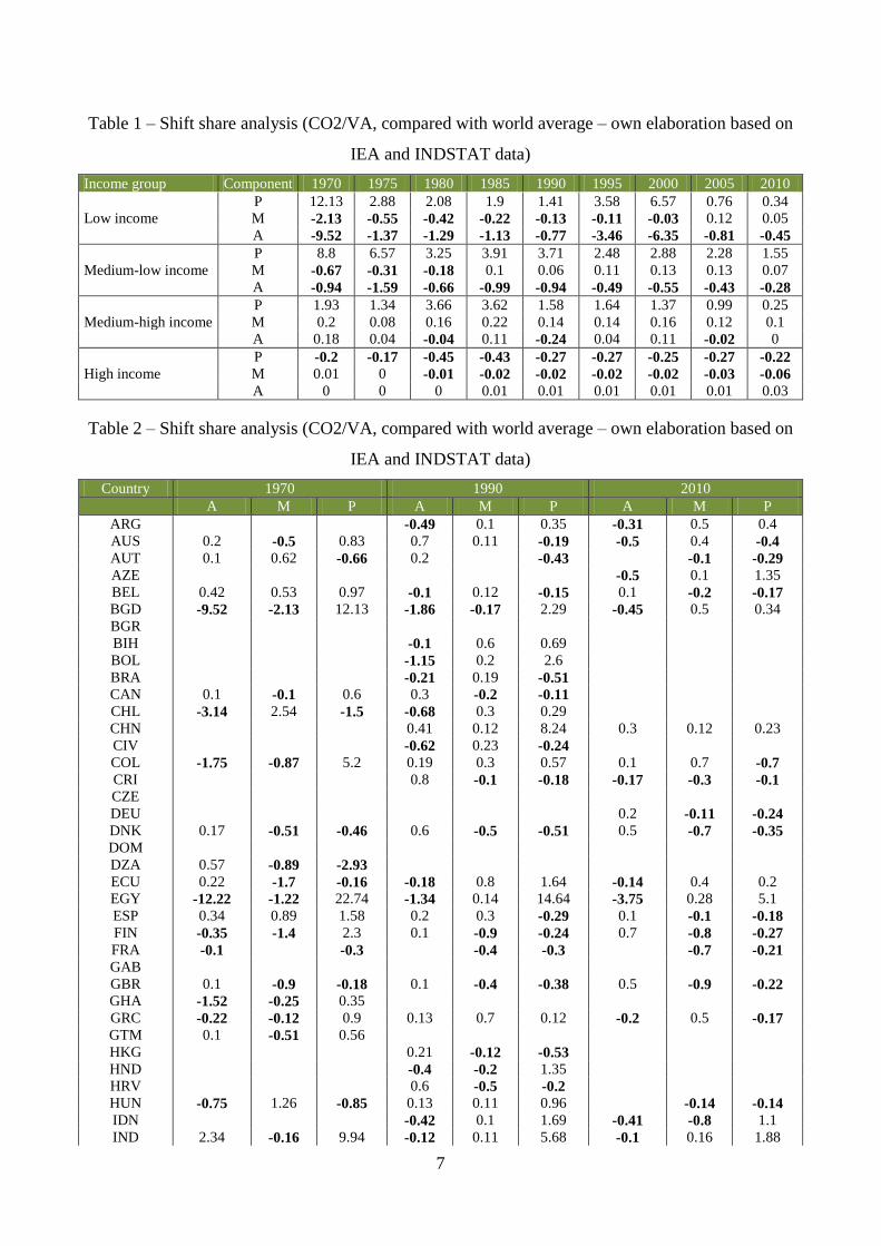
Table 1 – Shift share analysis (CO2/VA, compared with world average – own elaboration based on

IEA and INDSTAT data)

Income group Component 1970 1975 1980 1985 1990 1995 2000 2005 2010

P 12.13 2.88 2.08 1.9 1.41 3.58 6.57 0.76 0.34

Low income M -2.13 -0.55 -0.42 -0.22 -0.13 -0.11 -0.03 0.12 0.05

A -9.52 -1.37 -1.29 -1.13 -0.77 -3.46 -6.35 -0.81 -0.45

P 8.8 6.57 3.25 3.91 3.71 2.48 2.88 2.28 1.55

Medium-low income M -0.67 -0.31 -0.18 0.1 0.06 0.11 0.13 0.13 0.07

A -0.94 -1.59 -0.66 -0.99 -0.94 -0.49 -0.55 -0.43 -0.28

P 1.93 1.34 3.66 3.62 1.58 1.64 1.37 0.99 0.25

Medium-high income M 0.2 0.08 0.16 0.22 0.14 0.14 0.16 0.12 0.1

A 0.18 0.04 -0.04 0.11 -0.24 0.04 0.11 -0.02 0

P -0.2 -0.17 -0.45 -0.43 -0.27 -0.27 -0.25 -0.27 -0.22

High income M 0.01 0 -0.01 -0.02 -0.02 -0.02 -0.02 -0.03 -0.06

A 0 0 0 0.01 0.01 0.01 0.01 0.01 0.03

Table 2 – Shift share analysis (CO2/VA, compared with world average – own elaboration based on

IEA and INDSTAT data)

Country 1970 1990 2010

A M P A M P A M P

ARG

-0.49 0.1 0.35 -0.31 0.5 0.4

AUS 0.2 -0.5 0.83 0.7 0.11 -0.19 -0.5 0.4 -0.4

AUT 0.1 0.62 -0.66 0.2

-0.43

-0.1 -0.29

AZE

-0.5 0.1 1.35

BEL 0.42 0.53 0.97 -0.1 0.12 -0.15 0.1 -0.2 -0.17

BGD -9.52 -2.13 12.13 -1.86 -0.17 2.29 -0.45 0.5 0.34

BGR

BIH

-0.1 0.6 0.69

BOL

-1.15 0.2 2.6

BRA

-0.21 0.19 -0.51

CAN 0.1 -0.1 0.6 0.3 -0.2 -0.11

CHL -3.14 2.54 -1.5 -0.68 0.3 0.29

CHN

0.41 0.12 8.24 0.3 0.12 0.23

CIV

-0.62 0.23 -0.24

COL -1.75 -0.87 5.2 0.19 0.3 0.57 0.1 0.7 -0.7

CRI

0.8 -0.1 -0.18 -0.17 -0.3 -0.1

CZE

DEU

0.2 -0.11 -0.24

DNK 0.17 -0.51 -0.46 0.6 -0.5 -0.51 0.5 -0.7 -0.35

DOM

DZA 0.57 -0.89 -2.93

ECU 0.22 -1.7 -0.16 -0.18 0.8 1.64 -0.14 0.4 0.2

EGY -12.22 -1.22 22.74 -1.34 0.14 14.64 -3.75 0.28 5.1

ESP 0.34 0.89 1.58 0.2 0.3 -0.29 0.1 -0.1 -0.18

FIN -0.35 -1.4 2.3 0.1 -0.9 -0.24 0.7 -0.8 -0.27

FRA -0.1

-0.3

-0.4 -0.3

-0.7 -0.21

GAB

GBR 0.1 -0.9 -0.18 0.1 -0.4 -0.38 0.5 -0.9 -0.22

GHA -1.52 -0.25 0.35

GRC -0.22 -0.12 0.9 0.13 0.7 0.12 -0.2 0.5 -0.17

GTM 0.1 -0.51 0.56

HKG

0.21 -0.12 -0.53

HND

-0.4 -0.2 1.35

HRV

0.6 -0.5 -0.2

HUN -0.75 1.26 -0.85 0.13 0.11 0.96

-0.14 -0.14

IDN

-0.42 0.1 1.69 -0.41 -0.8 1.1

IND 2.34 -0.16 9.94 -0.12 0.11 5.68 -0.1 0.16 1.88

8

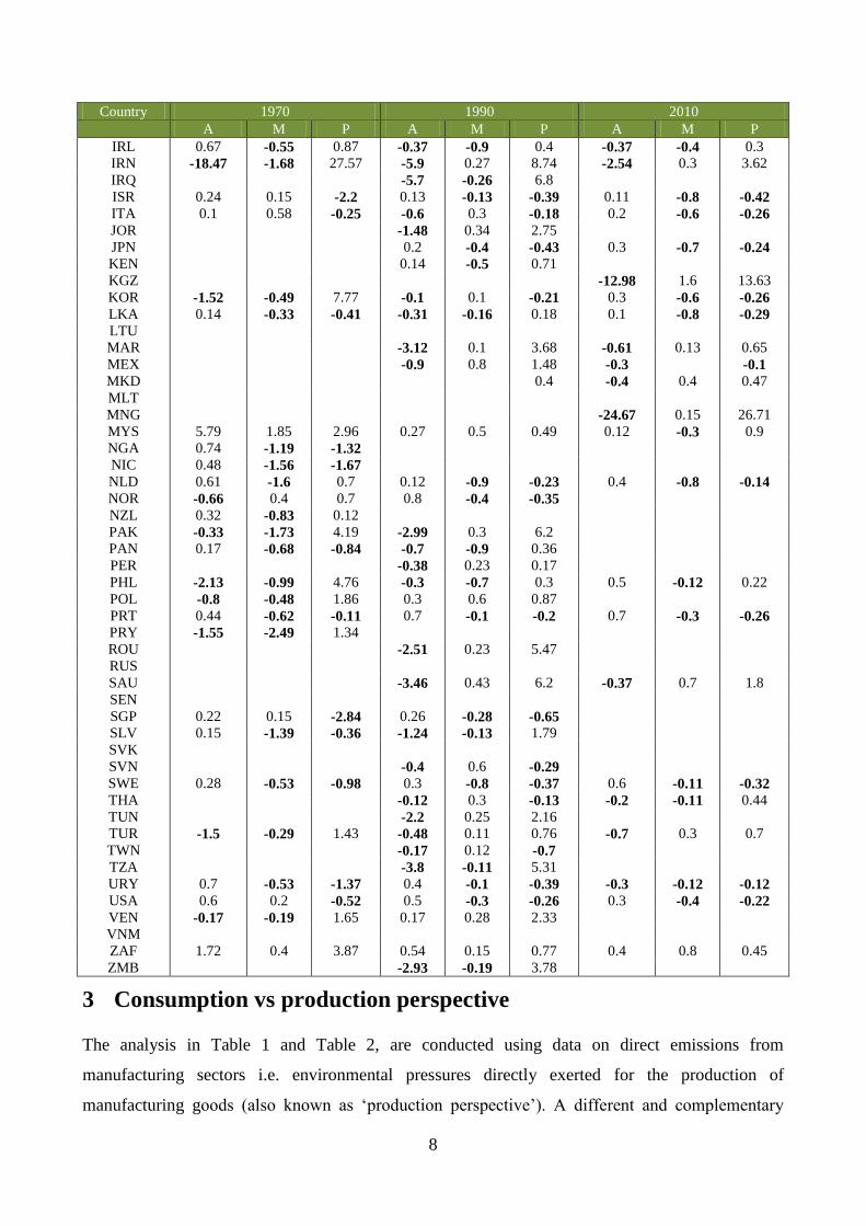
Country 1970 1990 2010

A M P A M P A M P

IRL 0.67 -0.55 0.87 -0.37 -0.9 0.4 -0.37 -0.4 0.3

IRN -18.47 -1.68 27.57 -5.9 0.27 8.74 -2.54 0.3 3.62

IRQ

-5.7 -0.26 6.8

ISR 0.24 0.15 -2.2 0.13 -0.13 -0.39 0.11 -0.8 -0.42

ITA 0.1 0.58 -0.25 -0.6 0.3 -0.18 0.2 -0.6 -0.26

JOR

-1.48 0.34 2.75

JPN

0.2 -0.4 -0.43 0.3 -0.7 -0.24

KEN

0.14 -0.5 0.71

KGZ

-12.98 1.6 13.63

KOR -1.52 -0.49 7.77 -0.1 0.1 -0.21 0.3 -0.6 -0.26

LKA 0.14 -0.33 -0.41 -0.31 -0.16 0.18 0.1 -0.8 -0.29

LTU

MAR

-3.12 0.1 3.68 -0.61 0.13 0.65

MEX

-0.9 0.8 1.48 -0.3

-0.1

MKD

0.4 -0.4 0.4 0.47

MLT

MNG

-24.67 0.15 26.71

MYS 5.79 1.85 2.96 0.27 0.5 0.49 0.12 -0.3 0.9

NGA 0.74 -1.19 -1.32

NIC 0.48 -1.56 -1.67

NLD 0.61 -1.6 0.7 0.12 -0.9 -0.23 0.4 -0.8 -0.14

NOR -0.66 0.4 0.7 0.8 -0.4 -0.35

NZL 0.32 -0.83 0.12

PAK -0.33 -1.73 4.19 -2.99 0.3 6.2

PAN 0.17 -0.68 -0.84 -0.7 -0.9 0.36

PER

-0.38 0.23 0.17

PHL -2.13 -0.99 4.76 -0.3 -0.7 0.3 0.5 -0.12 0.22

POL -0.8 -0.48 1.86 0.3 0.6 0.87

PRT 0.44 -0.62 -0.11 0.7 -0.1 -0.2 0.7 -0.3 -0.26

PRY -1.55 -2.49 1.34

ROU

-2.51 0.23 5.47

RUS

SAU

-3.46 0.43 6.2 -0.37 0.7 1.8

SEN

SGP 0.22 0.15 -2.84 0.26 -0.28 -0.65

SLV 0.15 -1.39 -0.36 -1.24 -0.13 1.79

SVK

SVN

-0.4 0.6 -0.29

SWE 0.28 -0.53 -0.98 0.3 -0.8 -0.37 0.6 -0.11 -0.32

THA

-0.12 0.3 -0.13 -0.2 -0.11 0.44

TUN

-2.2 0.25 2.16

TUR -1.5 -0.29 1.43 -0.48 0.11 0.76 -0.7 0.3 0.7

TWN

-0.17 0.12 -0.7

TZA

-3.8 -0.11 5.31

URY 0.7 -0.53 -1.37 0.4 -0.1 -0.39 -0.3 -0.12 -0.12

USA 0.6 0.2 -0.52 0.5 -0.3 -0.26 0.3 -0.4 -0.22

VEN -0.17 -0.19 1.65 0.17 0.28 2.33

VNM

ZAF 1.72 0.4 3.87 0.54 0.15 0.77 0.4 0.8 0.45

ZMB

-2.93 -0.19 3.78

3 Consumption vs production perspective

The analysis in Table 1 and Table 2, are conducted using data on direct emissions from

manufacturing sectors i.e. environmental pressures directly exerted for the production of

manufacturing goods (also known as ‘production perspective’). A different and complementary

9

approach can be derived considering, on the other side, the direct and indirect emissions occurring

along the supply chain, or the so called ‘consumption footprint’ or ‘consumption perspective’. This

second perspective is interesting because it calculates the total environmental pressure

corresponding to the final demand for selected consumption categories (here manufacturing goods

only) of a given country in a given year, tracking all emissions along the entire supply chain. In

other terms this means that it considers both direct and induced emissions, net of emission

associated to goods/service used as intermediate inputs in other sectors. Operatively, the main

complication when adopting this last approach is that consumption footprints data need to be

estimated. In our analysis, we rely on environmentally extended input-output (EEIO) modelling

starting from the EORA multi-regional input-output database (Lenzen et al., 2013)11

. We compare,

for the four income groups first and then for a selection of countries, the consumption and the

production perspective of manufacturing production/consumption. In particular, in Table 3, the first

five columns represent the ratio of emissions induced worldwide by domestic consumption of

manufacturing goods (‘consumption perspective’) that occurs in any sector (e.g. electricity

generation in the utilities sector purchased by the manufacturing sector) divided by the direct

emission of domestic production of manufacturing goods (‘production perspective’) either

consumed domestically or abroad as final goods or intermediates. In other terms, an higher level of

this indicator indicates that the analysed country releases more emissions to satisfy the final demand

of manufacturing goods as compared to direct emissions released by its manufacturing sector, or in

other terms that their consumption footprint of manufacturing goods is greater than their production

footprint.12

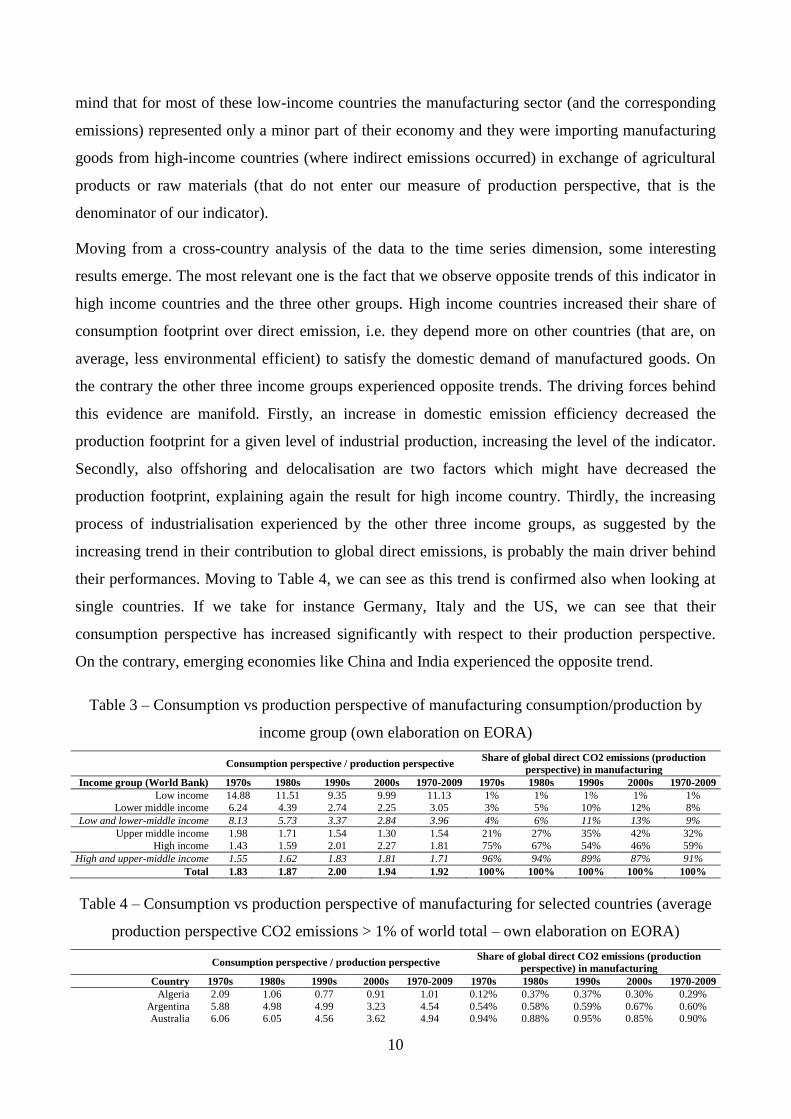
Looking at the results, several important considerations can be drawn. Firstly, in low and low-mid

income countries, the consumption footprint is much higher than the production footprint, which

means that they induce relatively more emissions worldwide with respect to the two other income

groups. This is obviously only a relative result, given by the comparison of the coefficients across

the groups. This evidence does not consider the size of emission of the two income groups. If we

look at the right five columns of table 3 in fact, we can easily note that despite their (relatively)

higher consumption footprint, low and mid low countries only account for a small share of total

CO2 direct emission, which increased from the 4% in 1970 to the 13% in the 2000. Even though this

result seems to contradict recent evidence about offshoring and carbon leakage, we should bear in

11

More details about data and methods for this section are reported in Appendix C. 12

The world-level weighted average of this indicator is not necessarily equal to one as the consumption perspective of

manufacturing goods on the one hand does not consider those manufacturing goods that serve to generate final products

and services in non-manufacturing industries and on the other hand it does account for emissions occurring to non-

manufacturing sectors that serve as suppliers of intermediate goods and services to the manufacturing sector.

10

mind that for most of these low-income countries the manufacturing sector (and the corresponding

emissions) represented only a minor part of their economy and they were importing manufacturing

goods from high-income countries (where indirect emissions occurred) in exchange of agricultural

products or raw materials (that do not enter our measure of production perspective, that is the

denominator of our indicator).

Moving from a cross-country analysis of the data to the time series dimension, some interesting

results emerge. The most relevant one is the fact that we observe opposite trends of this indicator in

high income countries and the three other groups. High income countries increased their share of

consumption footprint over direct emission, i.e. they depend more on other countries (that are, on

average, less environmental efficient) to satisfy the domestic demand of manufactured goods. On

the contrary the other three income groups experienced opposite trends. The driving forces behind

this evidence are manifold. Firstly, an increase in domestic emission efficiency decreased the

production footprint for a given level of industrial production, increasing the level of the indicator.

Secondly, also offshoring and delocalisation are two factors which might have decreased the

production footprint, explaining again the result for high income country. Thirdly, the increasing

process of industrialisation experienced by the other three income groups, as suggested by the

increasing trend in their contribution to global direct emissions, is probably the main driver behind

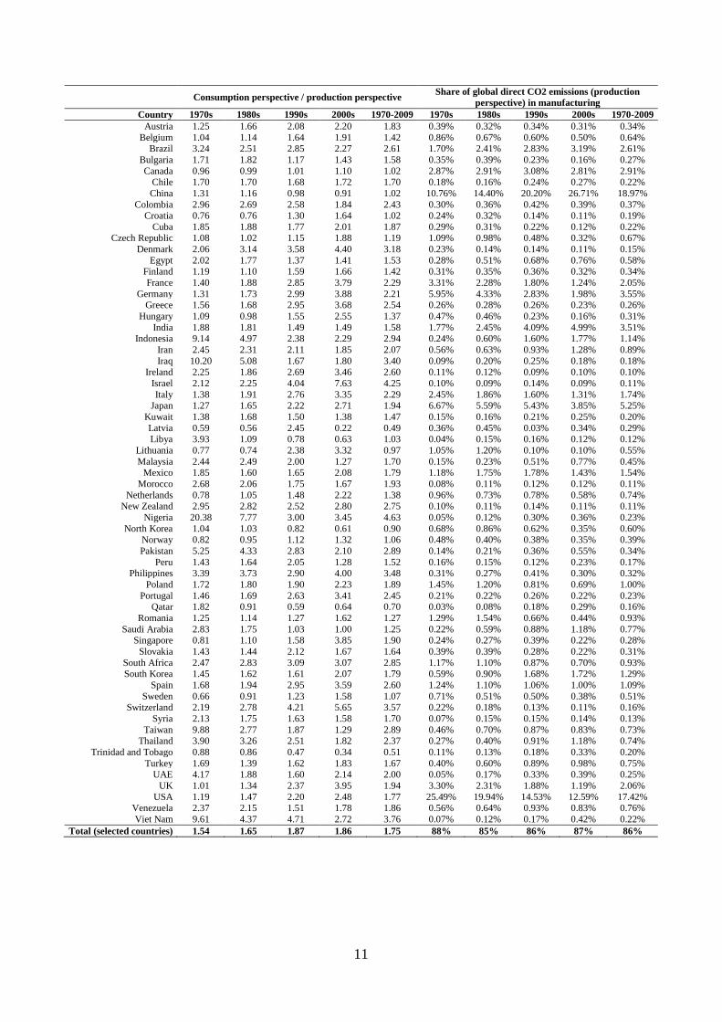
their performances. Moving to Table 4, we can see as this trend is confirmed also when looking at

single countries. If we take for instance Germany, Italy and the US, we can see that their

consumption perspective has increased significantly with respect to their production perspective.

On the contrary, emerging economies like China and India experienced the opposite trend.

Table 3 – Consumption vs production perspective of manufacturing consumption/production by

income group (own elaboration on EORA)

Consumption perspective / production perspective Share of global direct CO2 emissions (production

perspective) in manufacturing

Income group (World Bank) 1970s 1980s 1990s 2000s 1970-2009 1970s 1980s 1990s 2000s 1970-2009

Low income 14.88 11.51 9.35 9.99 11.13 1% 1% 1% 1% 1%

Lower middle income 6.24 4.39 2.74 2.25 3.05 3% 5% 10% 12% 8%

Low and lower-middle income 8.13 5.73 3.37 2.84 3.96 4% 6% 11% 13% 9%

Upper middle income 1.98 1.71 1.54 1.30 1.54 21% 27% 35% 42% 32%

High income 1.43 1.59 2.01 2.27 1.81 75% 67% 54% 46% 59%

High and upper-middle income 1.55 1.62 1.83 1.81 1.71 96% 94% 89% 87% 91%

Total 1.83 1.87 2.00 1.94 1.92 100% 100% 100% 100% 100%

Table 4 – Consumption vs production perspective of manufacturing for selected countries (average

production perspective CO2 emissions > 1% of world total – own elaboration on EORA)



Country 1970s 1980s 1990s 2000s 1970-2009 1970s 1980s 1990s 2000s 1970-2009

Algeria 2.09 1.06 0.77 0.91 1.01 0.12% 0.37% 0.37% 0.30% 0.29%

Argentina 5.88 4.98 4.99 3.23 4.54 0.54% 0.58% 0.59% 0.67% 0.60% Australia 6.06 6.05 4.56 3.62 4.94 0.94% 0.88% 0.95% 0.85% 0.90%

11



Country 1970s 1980s 1990s 2000s 1970-2009 1970s 1980s 1990s 2000s 1970-2009

Austria 1.25 1.66 2.08 2.20 1.83 0.39% 0.32% 0.34% 0.31% 0.34%

Belgium 1.04 1.14 1.64 1.91 1.42 0.86% 0.67% 0.60% 0.50% 0.64% Brazil 3.24 2.51 2.85 2.27 2.61 1.70% 2.41% 2.83% 3.19% 2.61%

Bulgaria 1.71 1.82 1.17 1.43 1.58 0.35% 0.39% 0.23% 0.16% 0.27%

Canada 0.96 0.99 1.01 1.10 1.02 2.87% 2.91% 3.08% 2.81% 2.91% Chile 1.70 1.70 1.68 1.72 1.70 0.18% 0.16% 0.24% 0.27% 0.22%

China 1.31 1.16 0.98 0.91 1.02 10.76% 14.40% 20.20% 26.71% 18.97%

Colombia 2.96 2.69 2.58 1.84 2.43 0.30% 0.36% 0.42% 0.39% 0.37% Croatia 0.76 0.76 1.30 1.64 1.02 0.24% 0.32% 0.14% 0.11% 0.19%

Cuba 1.85 1.88 1.77 2.01 1.87 0.29% 0.31% 0.22% 0.12% 0.22% Czech Republic 1.08 1.02 1.15 1.88 1.19 1.09% 0.98% 0.48% 0.32% 0.67%

Denmark 2.06 3.14 3.58 4.40 3.18 0.23% 0.14% 0.14% 0.11% 0.15%

Egypt 2.02 1.77 1.37 1.41 1.53 0.28% 0.51% 0.68% 0.76% 0.58% Finland 1.19 1.10 1.59 1.66 1.42 0.31% 0.35% 0.36% 0.32% 0.34%

France 1.40 1.88 2.85 3.79 2.29 3.31% 2.28% 1.80% 1.24% 2.05%

Germany 1.31 1.73 2.99 3.88 2.21 5.95% 4.33% 2.83% 1.98% 3.55% Greece 1.56 1.68 2.95 3.68 2.54 0.26% 0.28% 0.26% 0.23% 0.26%

Hungary 1.09 0.98 1.55 2.55 1.37 0.47% 0.46% 0.23% 0.16% 0.31%

India 1.88 1.81 1.49 1.49 1.58 1.77% 2.45% 4.09% 4.99% 3.51% Indonesia 9.14 4.97 2.38 2.29 2.94 0.24% 0.60% 1.60% 1.77% 1.14%

Iran 2.45 2.31 2.11 1.85 2.07 0.56% 0.63% 0.93% 1.28% 0.89%

Iraq 10.20 5.08 1.67 1.80 3.40 0.09% 0.20% 0.25% 0.18% 0.18% Ireland 2.25 1.86 2.69 3.46 2.60 0.11% 0.12% 0.09% 0.10% 0.10%

Israel 2.12 2.25 4.04 7.63 4.25 0.10% 0.09% 0.14% 0.09% 0.11%

Italy 1.38 1.91 2.76 3.35 2.29 2.45% 1.86% 1.60% 1.31% 1.74% Japan 1.27 1.65 2.22 2.71 1.94 6.67% 5.59% 5.43% 3.85% 5.25%

Kuwait 1.38 1.68 1.50 1.38 1.47 0.15% 0.16% 0.21% 0.25% 0.20%

Latvia 0.59 0.56 2.45 0.22 0.49 0.36% 0.45% 0.03% 0.34% 0.29% Libya 3.93 1.09 0.78 0.63 1.03 0.04% 0.15% 0.16% 0.12% 0.12%

Lithuania 0.77 0.74 2.38 3.32 0.97 1.05% 1.20% 0.10% 0.10% 0.55%

Malaysia 2.44 2.49 2.00 1.27 1.70 0.15% 0.23% 0.51% 0.77% 0.45% Mexico 1.85 1.60 1.65 2.08 1.79 1.18% 1.75% 1.78% 1.43% 1.54%

Morocco 2.68 2.06 1.75 1.67 1.93 0.08% 0.11% 0.12% 0.12% 0.11%

Netherlands 0.78 1.05 1.48 2.22 1.38 0.96% 0.73% 0.78% 0.58% 0.74% New Zealand 2.95 2.82 2.52 2.80 2.75 0.10% 0.11% 0.14% 0.11% 0.11%

Nigeria 20.38 7.77 3.00 3.45 4.63 0.05% 0.12% 0.30% 0.36% 0.23%

North Korea 1.04 1.03 0.82 0.61 0.90 0.68% 0.86% 0.62% 0.35% 0.60%

Norway 0.82 0.95 1.12 1.32 1.06 0.48% 0.40% 0.38% 0.35% 0.39%

Pakistan 5.25 4.33 2.83 2.10 2.89 0.14% 0.21% 0.36% 0.55% 0.34%

Peru 1.43 1.64 2.05 1.28 1.52 0.16% 0.15% 0.12% 0.23% 0.17% Philippines 3.39 3.73 2.90 4.00 3.48 0.31% 0.27% 0.41% 0.30% 0.32%

Poland 1.72 1.80 1.90 2.23 1.89 1.45% 1.20% 0.81% 0.69% 1.00%

Portugal 1.46 1.69 2.63 3.41 2.45 0.21% 0.22% 0.26% 0.22% 0.23% Qatar 1.82 0.91 0.59 0.64 0.70 0.03% 0.08% 0.18% 0.29% 0.16%

Romania 1.25 1.14 1.27 1.62 1.27 1.29% 1.54% 0.66% 0.44% 0.93%

Saudi Arabia 2.83 1.75 1.03 1.00 1.25 0.22% 0.59% 0.88% 1.18% 0.77% Singapore 0.81 1.10 1.58 3.85 1.90 0.24% 0.27% 0.39% 0.22% 0.28%

Slovakia 1.43 1.44 2.12 1.67 1.64 0.39% 0.39% 0.28% 0.22% 0.31%

South Africa 2.47 2.83 3.09 3.07 2.85 1.17% 1.10% 0.87% 0.70% 0.93% South Korea 1.45 1.62 1.61 2.07 1.79 0.59% 0.90% 1.68% 1.72% 1.29%

Spain 1.68 1.94 2.95 3.59 2.60 1.24% 1.10% 1.06% 1.00% 1.09%

Sweden 0.66 0.91 1.23 1.58 1.07 0.71% 0.51% 0.50% 0.38% 0.51% Switzerland 2.19 2.78 4.21 5.65 3.57 0.22% 0.18% 0.13% 0.11% 0.16%

Syria 2.13 1.75 1.63 1.58 1.70 0.07% 0.15% 0.15% 0.14% 0.13%

Taiwan 9.88 2.77 1.87 1.29 2.89 0.46% 0.70% 0.87% 0.83% 0.73% Thailand 3.90 3.26 2.51 1.82 2.37 0.27% 0.40% 0.91% 1.18% 0.74%

Trinidad and Tobago 0.88 0.86 0.47 0.34 0.51 0.11% 0.13% 0.18% 0.33% 0.20%

Turkey 1.69 1.39 1.62 1.83 1.67 0.40% 0.60% 0.89% 0.98% 0.75% UAE 4.17 1.88 1.60 2.14 2.00 0.05% 0.17% 0.33% 0.39% 0.25%

UK 1.01 1.34 2.37 3.95 1.94 3.30% 2.31% 1.88% 1.19% 2.06%

USA 1.19 1.47 2.20 2.48 1.77 25.49% 19.94% 14.53% 12.59% 17.42% Venezuela 2.37 2.15 1.51 1.78 1.86 0.56% 0.64% 0.93% 0.83% 0.76%

Viet Nam 9.61 4.37 4.71 2.72 3.76 0.07% 0.12% 0.17% 0.42% 0.22%

Total (selected countries) 1.54 1.65 1.87 1.86 1.75 88% 85% 86% 87% 86%

12

4 Environmental Kuznets Curves: achieving decoupling through

Industrial development and technology

The aim of the section is to analyse the impact of income and technological factors on the

environmental performance of developed and developing countries over time. We adopt as model

of reference the consolidated Environmental Kuznets curves framework (Marin & Mazzanti 2010).

We analyse EKC dynamics by using an unbalanced panel dataset which runs over 8 periods (5-

years length) from 1975 to 2010, thus covering the era of oil shocks, the 1992 Rio Convention, and

the post Kyoto Protocol period. We estimate EKC in a simple reduced form – by fixed effects panel

model - with the aim of testing non linearity with respect to GDP and the role of additional factors.

The estimated equation in a panel setting (i,t) is:

Where CO2 is the amount of CO2 emissions from manufacturing sectors (from the EORA database,

refer to Appendix C for further details). We will scrutinise both production, namely direct

emissions produced by economic activities, and consumption perspectives (refer to Appendix C for

further methodological details), namely direct and indirect emissions released to satisfy domestic

final demand for manufacturing goods, to shed light on ‘sustainable consumption and production’

issues (EEA 2014a). POP is population, GDP the income factor. Technological elements (TECH)

are proxied by the flow and stock of national patents (PATc, PATs) and spillovers (SPILL), built as

the average patenting intensity in neighbouring countries. Z hosts additional relevant factors such as

trade openness (TRADE) and inequality indexes (GINI). We use a parsimonious approach and

include in the regression the factors one by one in addition to the GDP-only baseline regression. We

finally include time dummies and comment on the role of temporal (fixed) effects; to verify whether

the significance of given factors (e.g. TRADE) is explained and absorbed by simple temporal

contents. Descriptive statistics are presented in the appendix (table C.1).

We present estimates for the whole sample of countries and – to offer more interesting and

eventually differentiated evidence - by world areas: Europe, Asia, Africa, America13

.

13

Since only eight countries from Oceania continent are included in the full sample, the restriction of the analysis to the

Oceania subsample would lead to biased and thus uninformative estimates. Therefore, it has not been possible to narrow

the EKC analysis to this area.

13

4.1 Whole sample14

The aggregate evidence for production perspective CO2 emissions of manufacturing sectors (Table

5) does not reject the hypothesis of a Kuznets like inverted U shape relationship, with a turning

point in terms of GDP per capita that lies in between the average and the maximum GDP per capita

observed in the sample15

.

While technological variables are not significant16

, both TRADE and Inequality appear to impact

negatively on emissions. The role of trade openness may reflect the fact that smaller open

economies tended to relocate heavier productions elsewhere. This gives relevance to the

consumption perspective. Inequality is more puzzling, since emissions per capita appear lower

when inequality is higher.

The evidence regarding the role played by technology deserves a comment. First, in the EKC

relevant literature, the inclusion of specific technological variables is not common. Technological

variables are often captured by fixed effects in different econometric contexts (Galeotti et al. 2006;

Vollebergh et al. 2009). Among EKC studies, we note Bouvier (2004), who find, for European and

North American countries for the period 1980-1986, that the scale effect outweighs the composition

and technology effects in the cases of carbon dioxide and volatile organic compounds, contrary to

sulphur dioxide. More recent evidence is provided by Auci & Becchetti (2006) and Auci & Trovato

(2011): the former ‘adjusts’ the EKC through the inclusion of variables that account for the energy

supply infrastructure and the industry mix. Though technology is explicitly considered, its empirical

inclusion finds proxies in the two mentioned factors. The latter paper, which analyses 25 EU

countries over 1997-2005, is instead one of the few that includes technological factors, namely

R&D. Authors state that: ‘As regards the influence of structural national or sectoral factors,

considering per capita GDP as an endogenous variable, the signs obtained are as we expect (…)

Technological progress induced by private R&D expenditure has a positive sign while the sign of

public R&D expenditure shows a puzzle result’.

Another issue is that we can only include total patents, not green ones. Total patents capture the

overall innovation capacity, both in brown and green economy. It would be nevertheless un-correct

14

The size of the panel considering all available countries, namely countries that present a reasonable coverage over

time (not all periods) and over the considered variables, is 1325. 15

We note that cubic effects are not significant here and for subsamples of countries. 16

In addition to patents, the share of R&D on GDP is also introduced as alternative covariate (results available on

request). R&D is similarly not significant across all specifications, and as expected it is positively correlated to patents.

There is some similarity with the methodological oriented evidence provided by Eberhardt et al. (2011), who highlight

the significance of factors which capture unobserved effects over R&D in the estimation of production functions.

Technological (and policy) factors are highly related to time events and dynamics. The inclusion of temporal effects

often brings about the irrelevance of those factors.

14

to include green patents even if they were available, since green patents are defined only for green

sectors and thus are more a proxy of the “greeness” of the sector than of the abating technology;

indeed, several emission reducing innovation are not patented in green sectors17

.

In addition, we note that overall worldwide evidence can hide heterogeneous conditions across

areas and countries. Policy implications are also more difficult to draw, without more specific

insights. On the role of unobserved heterogeneity factors see again Eberhardt et al. (2012), who

show that taking into account heterogeneity and cross section dependence shrinks and nullifies the

role of factors such as R&D.

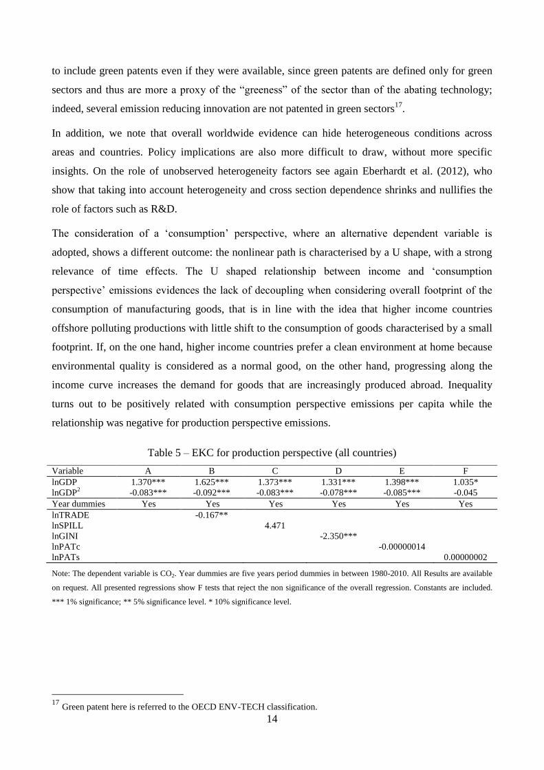
The consideration of a ‘consumption’ perspective, where an alternative dependent variable is

adopted, shows a different outcome: the nonlinear path is characterised by a U shape, with a strong

relevance of time effects. The U shaped relationship between income and ‘consumption

perspective’ emissions evidences the lack of decoupling when considering overall footprint of the

consumption of manufacturing goods, that is in line with the idea that higher income countries

offshore polluting productions with little shift to the consumption of goods characterised by a small

footprint. If, on the one hand, higher income countries prefer a clean environment at home because

environmental quality is considered as a normal good, on the other hand, progressing along the

income curve increases the demand for goods that are increasingly produced abroad. Inequality

turns out to be positively related with consumption perspective emissions per capita while the

relationship was negative for production perspective emissions.

Table 5 – EKC for production perspective (all countries)

Variable A B C D E F

lnGDP 1.370*** 1.625*** 1.373*** 1.331*** 1.398*** 1.035*

lnGDP2

-0.083*** -0.092*** -0.083*** -0.078*** -0.085*** -0.045

Year dummies Yes Yes Yes Yes Yes Yes lnTRADE -0.167**

lnSPILL 4.471

lnGINI -2.350***

lnPATc -0.00000014

lnPATs 0.00000002

Note: The dependent variable is CO2. Year dummies are five years period dummies in between 1980-2010. All Results are available

on request. All presented regressions show F tests that reject the non significance of the overall regression. Constants are included.

*** 1% significance; ** 5% significance level. * 10% significance level.

17

Green patent here is referred to the OECD ENV-TECH classification.

15

Table 6 – EKC for consumption perspective (all countries)


lnGDP -0.314** -0.024 -0.316** -0.471*** -0.313** 0.685

lnGDP2

0.030*** 0.038*** 0.031*** 0.043*** 0.037*** -0.019

Year dummies Yes Yes Yes Yes Yes Yes lnTRADE 0.068

lnSPILL -3.897

lnGINI 1.247***

lnPATc 0.0000001

lnPATs -0.0000002




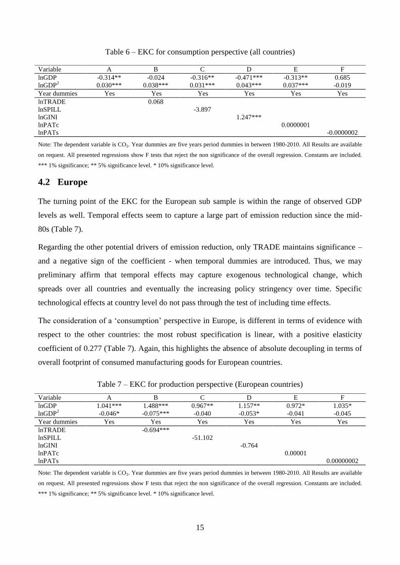
4.2 Europe

The turning point of the EKC for the European sub sample is within the range of observed GDP

levels as well. Temporal effects seem to capture a large part of emission reduction since the mid-

80s (Table 7).

Regarding the other potential drivers of emission reduction, only TRADE maintains significance –

and a negative sign of the coefficient - when temporal dummies are introduced. Thus, we may

preliminary affirm that temporal effects may capture exogenous technological change, which

spreads over all countries and eventually the increasing policy stringency over time. Specific

technological effects at country level do not pass through the test of including time effects.

The consideration of a ‘consumption’ perspective in Europe, is different in terms of evidence with

respect to the other countries: the most robust specification is linear, with a positive elasticity

coefficient of 0.277 (Table 7). Again, this highlights the absence of absolute decoupling in terms of

overall footprint of consumed manufacturing goods for European countries.

Table 7 – EKC for production perspective (European countries)


lnGDP 1.041*** 1.488*** 0.967** 1.157** 0.972* 1.035*

lnGDP2

-0.046* -0.075*** -0.040 -0.053* -0.041 -0.045

Year dummies Yes Yes Yes Yes Yes Yes lnTRADE -0.694***

lnSPILL -51.102

lnGINI -0.764

lnPATc 0.00001

lnPATs 0.00000002




16

Table 8 – EKC for consumption perspective (European countries)


lnGDP 0.272*** 0.273*** 0.277*** 0.288*** 0.342*** 0.329***

lnGDP2

Year dummies Yes Yes Yes Yes Yes Yes lnTRADE -0.209*

lnSPILL -10.772

lnGINI -0.348

lnPATc 0.00000002

lnPATs -0.0000002



*** 1% significance; ** 5% significance level. * 10% significance level. lnGDP2 is not significant.

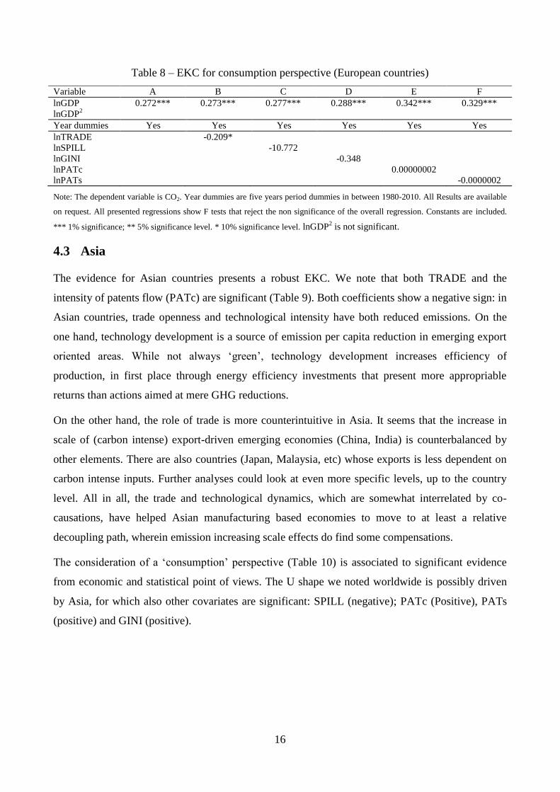
4.3 Asia

The evidence for Asian countries presents a robust EKC. We note that both TRADE and the

intensity of patents flow (PATc) are significant (Table 9). Both coefficients show a negative sign: in

Asian countries, trade openness and technological intensity have both reduced emissions. On the

one hand, technology development is a source of emission per capita reduction in emerging export

oriented areas. While not always ‘green’, technology development increases efficiency of

production, in first place through energy efficiency investments that present more appropriable

returns than actions aimed at mere GHG reductions.

On the other hand, the role of trade is more counterintuitive in Asia. It seems that the increase in

scale of (carbon intense) export-driven emerging economies (China, India) is counterbalanced by

other elements. There are also countries (Japan, Malaysia, etc) whose exports is less dependent on

carbon intense inputs. Further analyses could look at even more specific levels, up to the country

level. All in all, the trade and technological dynamics, which are somewhat interrelated by co-

causations, have helped Asian manufacturing based economies to move to at least a relative

decoupling path, wherein emission increasing scale effects do find some compensations.

The consideration of a ‘consumption’ perspective (Table 10) is associated to significant evidence

from economic and statistical point of views. The U shape we noted worldwide is possibly driven

by Asia, for which also other covariates are significant: SPILL (negative); PATc (Positive), PATs

(positive) and GINI (positive).

17

Table 9 – EKC for production perspective (Asian countries)


lnGDP 1.240*** 1.965*** 1.346*** 1.580*** 1.614*** 1.514***

lnGDP2

-0.067*** -0.097*** -0.071*** -0.088*** -0.077*** -0.071***

Year dummies Yes Yes Yes Yes Yes Yes lnTRADE -0.330**

lnSPILL 39.701

lnGINI -1.094*

lnPATc -0.0000009*

lnPATs -0.0000002*




Table 10 – EKC for consumption perspective (Asian countries)


lnGDP -0.709*** -0.253*** -0.840*** -1.085*** -0.699*** -0.588***

lnGDP2

0.0466*** 0.053*** 0.051*** 0.071*** 0.049** 0.042**

Year dummies Yes Yes Yes Yes Yes Yes lnTRADE 0.187**

lnSPILL -58.578**

lnGINI 1.805**

lnPATc 0.00001**

lnPATs 0.0000003*




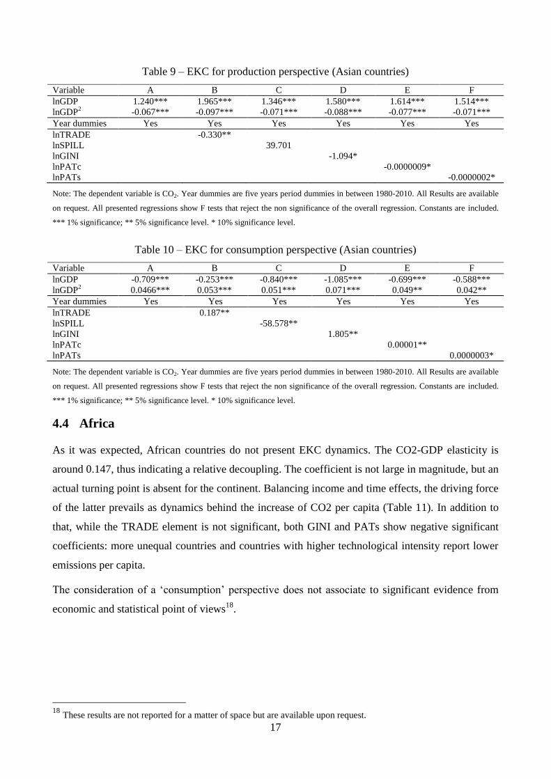
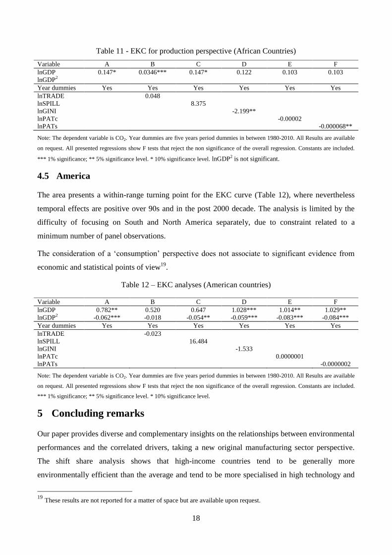
4.4 Africa

As it was expected, African countries do not present EKC dynamics. The CO2-GDP elasticity is

around 0.147, thus indicating a relative decoupling. The coefficient is not large in magnitude, but an

actual turning point is absent for the continent. Balancing income and time effects, the driving force

of the latter prevails as dynamics behind the increase of CO2 per capita (Table 11). In addition to

that, while the TRADE element is not significant, both GINI and PATs show negative significant

coefficients: more unequal countries and countries with higher technological intensity report lower

emissions per capita.

The consideration of a ‘consumption’ perspective does not associate to significant evidence from

economic and statistical point of views18

.

18

These results are not reported for a matter of space but are available upon request.

18

Table 11 - EKC for production perspective (African Countries)


lnGDP 0.147* 0.0346*** 0.147* 0.122 0.103 0.103

lnGDP2

Year dummies Yes Yes Yes Yes Yes Yes lnTRADE 0.048

lnSPILL 8.375

lnGINI -2.199**

lnPATc -0.00002

lnPATs -0.000068**



*** 1% significance; ** 5% significance level. * 10% significance level. lnGDP2 is not significant.

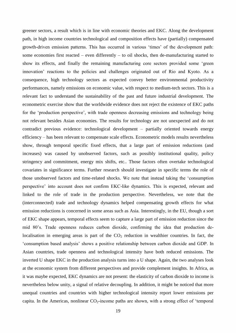
4.5 America

The area presents a within-range turning point for the EKC curve (Table 12), where nevertheless

temporal effects are positive over 90s and in the post 2000 decade. The analysis is limited by the

difficulty of focusing on South and North America separately, due to constraint related to a

minimum number of panel observations.

The consideration of a ‘consumption’ perspective does not associate to significant evidence from

economic and statistical points of view19

.

Table 12 – EKC analyses (American countries)


lnGDP 0.782** 0.520 0.647 1.028*** 1.014** 1.029**

lnGDP2

-0.062*** -0.018 -0.054** -0.059*** -0.083*** -0.084***

Year dummies Yes Yes Yes Yes Yes Yes lnTRADE -0.023

lnSPILL 16.484

lnGINI -1.533

lnPATc 0.0000001

lnPATs -0.0000002




5 Concluding remarks

Our paper provides diverse and complementary insights on the relationships between environmental

performances and the correlated drivers, taking a new original manufacturing sector perspective.

The shift share analysis shows that high-income countries tend to be generally more

environmentally efficient than the average and tend to be more specialised in high technology and

19

These results are not reported for a matter of space but are available upon request.

19

greener sectors, a result which is in line with economic theories and EKC. Along the development

path, in high income countries technological and composition effects have (partially) compensated

growth-driven emission patterns. This has occurred in various ‘times’ of the development path:

some economies first reacted – even differently – to oil shocks, then de-manufacturing started to

show its effects, and finally the remaining manufacturing core sectors provided some ‘green

innovation’ reactions to the policies and challenges originated out of Rio and Kyoto. As a

consequence, high technology sectors as expected convey better environmental productivity

performances, namely emissions on economic value, with respect to medium-tech sectors. This is a

relevant fact to understand the sustainability of the past and future industrial development. The

econometric exercise show that the worldwide evidence does not reject the existence of EKC paths

for the ‘production perspective’, with trade openness decreasing emissions and technology being

not relevant besides Asian economies. The results for technology are not unexpected and do not

contradict previous evidence: technological development – partially oriented towards energy

efficiency – has been relevant to compensate scale effects. Econometric models results nevertheless

show, through temporal specific fixed effects, that a large part of emission reductions (and

increases) was caused by unobserved factors, such as possibly institutional quality, policy

stringency and commitment, energy mix shifts, etc.. Those factors often overtake technological

covariates in significance terms. Further research should investigate in specific terms the role of

those unobserved factors and time-related shocks. We note that instead taking the ‘consumption

perspective’ into account does not confirm EKC-like dynamics. This is expected, relevant and

linked to the role of trade in the production perspective. Nevertheless, we note that the

(interconnected) trade and technology dynamics helped compensating growth effects for what

emission reductions is concerned in some areas such as Asia. Interestingly, in the EU, though a sort

of EKC shape appears, temporal effects seem to capture a large part of emission reduction since the

mid 80’s. Trade openness reduces carbon dioxide, confirming the idea that production de-

localisation in emerging areas is part of the CO2 reduction in wealthier countries. In fact, the

‘consumption based analysis’ shows a positive relationship between carbon dioxide and GDP. In

Asian countries, trade openness and technological intensity have both reduced emissions. The

inverted U shape EKC in the production analysis turns into a U shape. Again, the two analyses look

at the economic system from different perspectives and provide complement insights. In Africa, as

it was maybe expected, EKC dynamics are not present: the elasticity of carbon dioxide to income is

nevertheless below unity, a signal of relative decoupling. In addition, it might be noticed that more

unequal countries and countries with higher technological intensity report lower emissions per

capita. In the Americas, nonlinear CO2-income paths are shown, with a strong effect of ‘temporal

20

factors’ again, that seem to cause an increase in emissions in the last two decades, which is similar

to what temporal factors highlight for the EU. The hypothesis that technology drives down CO2 to

compensate scale effect is more relevant for developing and emerging economies, while in the EU

trade is a determinant factor. When technology matters, it is not due to spillover effects, though this

evidence needs further (spatially oriented) research. Temporal related factors often show greater

relevance. This opens the way to further analyses and introduction of additional carbon dioxide

drivers, e.g. policies. The nonlinear EKC path do not exists when we introduce a consumption

rather than a production perspective. In the most relevant cases, the EU presents a positive link

between emissions and economic value, while Asia presents a U shape opposite to the EKC

hypothesis. This shows that the EKC evidence we may find heavily rely on the ‘production oriented

approach’.

Finally, regarding the specific comparison between consumption and production perspective

through input output techniques, we further note that the ratio between the footprint of domestic

consumption of manufacturing goods and the domestic direct emissions of manufacturing sectors

(namely, consumption and production perspectives) is increasing when moving from high-income

countries to low-income countries, due to the greater development of the manufacturing sector in

high-income countries. However, when looking at the dynamics of this indicator we observe a

progressive convergence of low-income countries (due to increased importance of manufacturing in

these countries) towards high-income countries, in which a rather stable dynamics of consumption

of manufacturing goods has been accompanied by the offshoring of manufacturing activities

towards lower-income countries.

21

References

Auci, S. & Becchetti, L., 2006. The instability of the adjusted and unadjusted environmental

Kuznets curves. Ecological Economics, 60(1), pp.282–298.

Auci, S. & Trovato, G., 2011. The environmental Kuznets curve within European countries and

sectors: greenhouse emission, production function and technology, Munich.

Baumol, W.J., 1967. Macroeconomics of Unbalanced Growth: The Anatomy of Urban Crisis.

American Economic Review, 57, pp.415–426.

Bouvier, R. a, 2004. Air Pollution and Per Capita Income, Amherst.

Costantini, V. & Mazzanti, M., 2012. On the green and innovative side of trade competitiveness?

The impact of environmental policies and innovation on EU exports. Research Policy, 41(1),

pp.132–153.

Costantini, V., Mazzanti, M. & Montini, A., 2013. Environmental performance, innovation and

spillovers. Evidence from a regional NAMEA. Ecological Economics, 89, pp.101–114.

Costantini, V., Mazzanti, M. & Montini, A., 2011. Hybrid Economic Environmental Accounts,

London: Routledge.

Eberhardt, M., Helmers, C. & Strauss, H., 2012. Do Spillovers Matter When Estimating Private

Returns to R&D? Review of Economics and Statistics, 95(May), pp 436-448.

EEA, 2014a. Achieving a green economy transition in Europe, Copenhagen.

EEA, 2014b. Resource-efficient green economy and EU policies, Copenhagen.

EEA, 2013. Towards the green economy, Cophenhagen.

Esteban, J., 2000. Regional convergence in Europe and the industry mix: A shift-share analysis.

Regional Science and Urban Economics, 30, pp.353–364.

Galeotti, M., Lanza, A. & Pauli, F., 2006. Reassessing the environmental Kuznets curve for CO2

emissions: A robustness exercise. Ecological Economics, 57(1), pp.152–163.

Gilli, M., Mazzanti, M. & Nicolli, F., 2013. Sustainability and competitiveness in evolutionary

perspectives: Environmental innovations, structural change and economic dynamics in the EU.

The Journal of Socio-Economics, 45, pp.204–215.

Keller, W. & Levinson, A., 2002. Pollution Abatement Costs and Foreign Direct Investment

Inflows to U.S. States. Review of Economics and Statistics, 84(4), pp.691–703.

Lenzen, M. et al., 2013. Buildin EORA: a global multi-region input-output databaseat high country

and sector resolution. Economic System Research, 25(1).

Lenzen, M. et al., 2012. Mapping the structure of the world economy. Environmental Science and

Technology, 46, pp.8374–8381.

Levinson, A., 2009. Pollution and international trade in services, NBER, Working Paper no.14963.

Marin, G. & Mazzanti, M., 2010. The evolution of environmental and labor productivity dynamics.

Journal of Evolutionary Economics, 23(2), pp.357–399.

Marin, G., Mazzanti, M. & Montini, A., 2012. Linking NAMEA and Input output for “consumption

vs. production perspective” analyses. Evidence on emission efficiency and aggregation biases

using the Italian and Spanish environmental accounts. Ecological Economics, 74, pp.71–84.

Martinez-Zarzoso, I., Bengochea-Morancho, A. & Morales Lage, R., 2007. The Impact of

Population on CO2 Emissions: Evidence from European Countries. Environmental and

Resource Economics, 38, pp.497–512.

22

Mazzanti, M. & Montini, A., 2010. Embedding the drivers of emission efficiency at regional level

— Analyses of NAMEA data. Ecological Economics, 69(12), pp.2457–2467.

Mazzanti, M. & Musolesi, A., 2013. Non-linearity, heterogeneity and unobserved effects in the

CO2-income relation for advanced countries, FEEM, Working Paper no. 44.

Musolesi, A. & Mazzanti, M., 2014. Nonlinearity, heterogeneity and unobserved effects in the

carbon dioxide emissions-economic development relation for advanced countries. Studies in

Nonlinear Dynamics & Econometrics, 18(5), p.21.

Musolesi, A., Mazzanti, M. & Zoboli, R., 2010. A panel data heterogeneous Bayesian estimation of

environmental Kuznets curves for CO 2 emissions. Applied Economics, 42, pp.2275–2287.

Rodrik, D., 2013. Unconditional convergence in manufacturing. Quarterly Journal of Economics,

128(1), pp.165–204.

Serrano, M. & Dietzenbacher, E., 2010. Responsibility and trade emission balances: An evaluation

of approaches. Ecological Economics, 69(11), pp.2224–2232.

Vollebergh, H. & Kemfert, C., 2005. The role of technological change for a sustainable

development. Ecological Economics, 54, pp.133–147.

Vollebergh, H.R.J., Melenberg, B. & Dijkgraaf, E., 2009. Identifying reduced-form relations with

panel data: The case of pollution and income. Journal of Environmental Economics and

Management, 58(1), pp.27–42.

Wagner, U.J. & Timmins, C.D., 2008. Agglomeration Effects in Foreign Direct Investment and the

Pollution Haven Hypothesis. Environmental and Resource Economics, 43(2), pp.231–256.

23

Appendix A: IEA and INDSTAT databases – Online Supplementary

Material

The empirical analysis reported in shift share analysis of the current article is based on two different

databases. CO2 air emissions deriving from the combustion of fossil fuels are retrieved from the

corresponding database maintained by the International Energy Agency (IEA). Emissions are

reported in millions of tons. However, where emissions are smaller than 100,000 tons, they are

rounded to zero. For simplicity, with little influence on results, we set these values to 50,000 tons

given that for both the decomposition analysis and the shift share analysis values for emissions

should be strictly positive. In any case, being aggregate results weighted by the size of sectors and

countries, these assumptions have little influence on aggregate results. To increase the time and

country coverage, we linearly interpolated information on emissions given that decomposition

exercises require that information is available for all sectors in a countries for two different points

in time.

Real value added in US dollars by manufacturing sectors (ISIC Rev 3.1) come from the INDSTAT2

database maintained by the UNIDO. Value added in nominal terms by sector, for which we have

the greater coverage in INDSTAT2, is deflated to 2005 prices (US$) using the deflator for

manufacturing industries provided by the United Nations Statistics Division20

. Also for what

concerns value added, we perform linear interpolations to increase the coverage.

Finally, to increase coverage and reduce the potential issue of measurement errors, we do not use

yearly information but five years windows, in which the value of value added and emissions for the

specific year (e.g. 1980) is computed as the simple average of all available years between 1978 and

1982.

To combine the two datasets and to cover a sufficient number of countries and time period, we

aggregate sectors as follows:

20

http://unstats.un.org/unsd/snaama/dnllist.asp

http://unstats.un.org/unsd/snaama/dnllist.asp

24

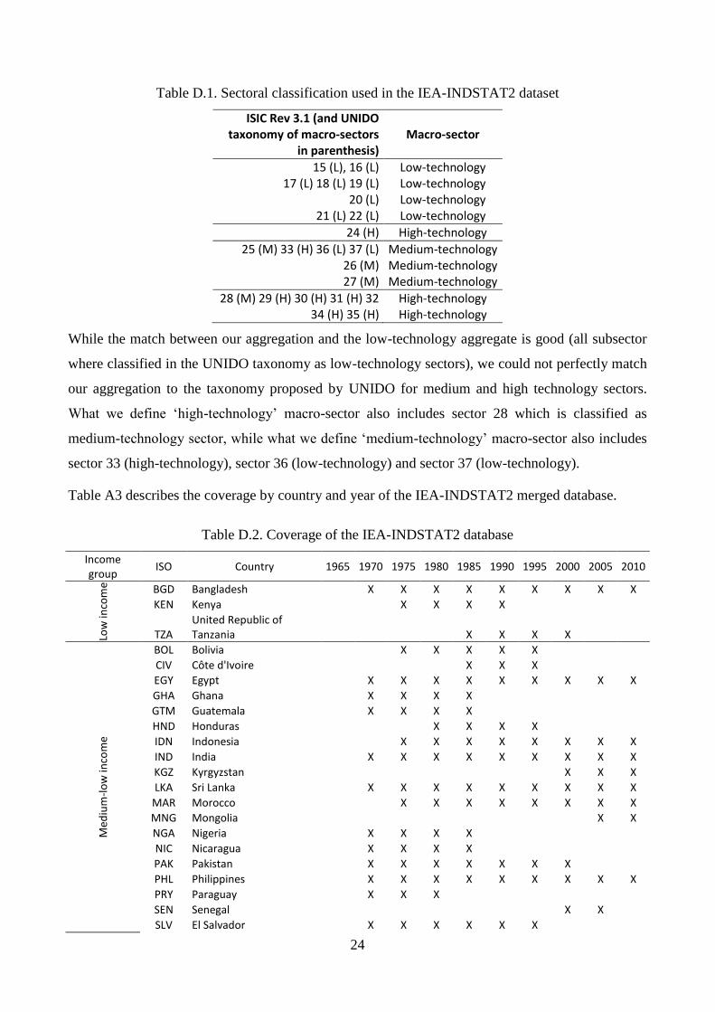
Table D.1. Sectoral classification used in the IEA-INDSTAT2 dataset

ISIC Rev 3.1 (and UNIDO taxonomy of macro-sectors

in parenthesis) Macro-sector

15 (L), 16 (L) Low-technology 17 (L) 18 (L) 19 (L) Low-technology

20 (L) Low-technology 21 (L) 22 (L) Low-technology

24 (H) High-technology

25 (M) 33 (H) 36 (L) 37 (L) Medium-technology 26 (M) Medium-technology 27 (M) Medium-technology

28 (M) 29 (H) 30 (H) 31 (H) 32 High-technology 34 (H) 35 (H) High-technology

While the match between our aggregation and the low-technology aggregate is good (all subsector

where classified in the UNIDO taxonomy as low-technology sectors), we could not perfectly match

our aggregation to the taxonomy proposed by UNIDO for medium and high technology sectors.

What we define ‘high-technology’ macro-sector also includes sector 28 which is classified as

medium-technology sector, while what we define ‘medium-technology’ macro-sector also includes

sector 33 (high-technology), sector 36 (low-technology) and sector 37 (low-technology).

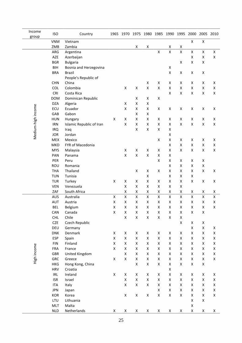
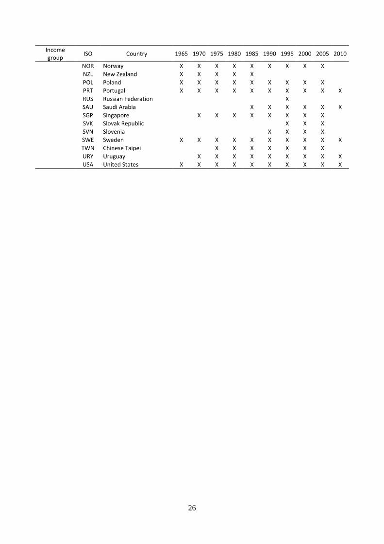
Table A3 describes the coverage by country and year of the IEA-INDSTAT2 merged database.

Table D.2. Coverage of the IEA-INDSTAT2 database

Income group

ISO Country 1965 1970 1975 1980 1985 1990 1995 2000 2005 2010

Low

inco

me

BGD Bangladesh

X X X X X X X X X

KEN Kenya

X X X X

TZA United Republic of Tanzania X X X X

Med

ium

-lo

w in

com

e

BOL Bolivia

X X X X X

CIV Côte d'Ivoire

X X X

EGY Egypt

X X X X X X X X X

GHA Ghana

X X X X

GTM Guatemala

X X X X

HND Honduras

X X X X

IDN Indonesia

X X X X X X X X

IND India

X X X X X X X X X

KGZ Kyrgyzstan

X X X

LKA Sri Lanka

X X X X X X X X X

MAR Morocco

X X X X X X X X

MNG Mongolia

X X

NGA Nigeria

X X X X

NIC Nicaragua

X X X X

PAK Pakistan

X X X X X X X

PHL Philippines

X X X X X X X X X

PRY Paraguay

X X X

SEN Senegal

X X

SLV El Salvador

X X X X X X

25

Income group

ISO Country 1965 1970 1975 1980 1985 1990 1995 2000 2005 2010

VNM Vietnam

X X

ZMB Zambia X X X X

Med

ium

-hig

h in

com

e

ARG Argentina

X X X X X X

AZE Azerbaijan

X X X

BGR Bulgaria

X X X

BIH Bosnia and Herzegovina

X

BRA Brazil

X X X X

CHN People's Republic of China

X X X X X X X

COL Colombia

X X X X X X X X X

CRI Costa Rica

X X X X X

DOM Dominican Republic

X X X

DZA Algeria

X X X

ECU Ecuador

X X X X X X X X X

GAB Gabon

X X

HUN Hungary X X X X X X X X X X

IRN Islamic Republic of Iran

X X X X X X X X X

IRQ Iraq

X X X X

JOR Jordan

X

MEX Mexico

X X X X X X

MKD FYR of Macedonia

X X X X X

MYS Malaysia

X X X X X X X X X

PAN Panama

X X X X X

PER Peru

X X X X X

ROU Romania

X X X X

THA Thailand

X X X X X X X X

TUN Tunisia

X

X X X

TUR Turkey X X X X X X X X X X

VEN Venezuela

X X X X X X

ZAF South Africa X X X X X X X X X

Hig

h in

com

e

AUS Australia X X X X X X X X X X

AUT Austria X X X X X X X X X X

BEL Belgium X X X X X X X X X X

CAN Canada X X X X X X X X X

CHL Chile

X X X X X X

CZE Czech Republic

X X X

DEU Germany

X X X

DNK Denmark X X X X X X X X X X

ESP Spain X X X X X X X X X X

FIN Finland X X X X X X X X X X

FRA France X X X X X X X X X X

GBR United Kingdom

X X X X X X X X X

GRC Greece X X X X X X X X X X

HKG Hong Kong, China

X X X X X X X

HRV Croatia

X

IRL Ireland X X X X X X X X X X

ISR Israel

X X X X X X X X X

ITA Italy

X X X X X X X X X

JPN Japan

X X X X X X

KOR Korea

X X X X X X X X X

LTU Lithuania

X X

MLT Malta

X

NLD Netherlands X X X X X X X X X X

26

Income group

ISO Country 1965 1970 1975 1980 1985 1990 1995 2000 2005 2010

NOR Norway X X X X X X X X X

NZL New Zealand X X X X X

POL Poland X X X X X X X X X

PRT Portugal X X X X X X X X X X

RUS Russian Federation

X

SAU Saudi Arabia

X X X X X X

SGP Singapore

X X X X X X X X

SVK Slovak Republic

X X X

SVN Slovenia

X X X X

SWE Sweden X X X X X X X X X X

TWN Chinese Taipei

X X X X X X X

URY Uruguay

X X X X X X X X X

USA United States X X X X X X X X X X

27

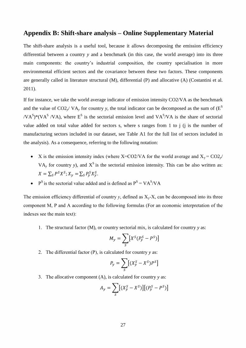
Appendix B: Shift-share analysis – Online Supplementary Material

The shift-share analysis is a useful tool, because it allows decomposing the emission efficiency

differential between a country y and a benchmark (in this case, the world average) into its three

main components: the country’s industrial composition, the country specialisation in more

environmental efficient sectors and the covariance between these two factors. These components

are generally called in literature structural (M), differential (P) and allocative (A) (Costantini et al.

2011).

If for instance, we take the world average indicator of emission intensity CO2/VA as the benchmark

and the value of CO2y/ VAy for country y, the total indicator can be decomposed as the sum of (ES

/VAS)*(VA

S /VA), where E

S is the sectorial emission level and VA

S/VA is the share of sectorial

value added on total value added for sectors s, where s ranges from 1 to j (j is the number of

manufacturing sectors included in our dataset, see Table A1 for the full list of sectors included in

the analysis). As a consequence, referring to the following notation:

X is the emission intensity index (where X=CO2/VA for the world average and Xy = CO2y/

VAy for country y), and XS

is the sectorial emission intensity. This can be also written as:

PS

is the sectorial value added and is defined as PS = VA

S/VA

The emission efficiency differential of country y, defined as Xy-X, can be decomposed into its three

component M, P and A according to the following formulas (For an economic interpretation of the

indexes see the main text):

1. The structural factor (M), or country sectorial mix, is calculated for country y as:

2. The differential factor (P), is calculated for country y as:

3. The allocative component (A), is calculated for country y as:

28

Appendix C: Consumption perspective and the EORA database –

Online Supplementary Material

Information on CO2 emissions used in analysis of section 3 and 4 is based on the EORA

(http://worldmrio.com/) database (Lenzen et al. 2012; Lenzen et al. 2013). The database provides

estimates of sectoral direct CO2 emissions together with year-specific world input output tables for

187 countries, 26 sectors (7 of which pertaining to manufacturing sectors) over the period 1970-

2011.

We build two different indicators of emissions based on this base of data. The first is labelled as

‘production perspective emissions’ and refer to direct emissions by manufacturing sectors due to

their production activity. This indicator reflects the pressures exerted by the manufacturing sector as

a whole no matter where the goods produced are then consumed and with no consideration of

indirect emissions (i.e. from other sectors and, eventually, other countries) occurred along the

supply chain to produce these goods.

The second indicator, labelled as ‘consumption perspective emissions’, measures the amount of

emissions needed (directly and indirectly, at home and abroad) to satisfy the domestic demand for

manufacturing goods. The indicator is built by exploiting the information from the world input

output tables of EORA that allow to account for emissions occurring along the whole world supply

chain of domestically-consumed manufacturing goods. We adopt the common approach described

by Serrano & Dietzenbacher (2010), based on the Leontief input output model, to compute

‘consumption perspective emissions’.

The world totals for the two indicators would not necessarily coincide. This is because while

‘production perspective emissions’ only consider direct emissions from manufacturing sectors,

‘consumption perspective emissions’ include indirect emissions that occur in other relevant sectors

(e.g. the power generation sector) and are embodied in manufacturing goods while it excludes

emissions corresponding to those manufacturing products that are used as intermediate inputs for

other non-manufacturing sectors.

29

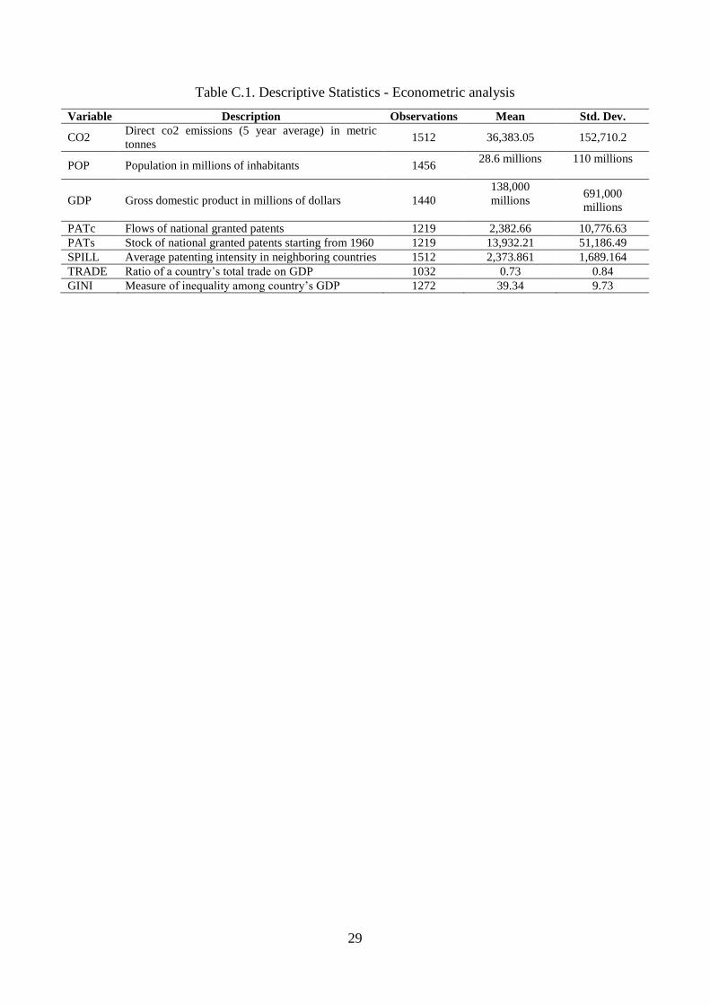
Table C.1. Descriptive Statistics - Econometric analysis

Variable Description Observations Mean Std. Dev.

CO2 Direct co2 emissions (5 year average) in metric

tonnes 1512 36,383.05 152,710.2

POP Population in millions of inhabitants 1456 28.6 millions

110 millions

GDP Gross domestic product in millions of dollars 1440

138,000

millions

691,000

millions

PATc Flows of national granted patents 1219 2,382.66 10,776.63

PATs Stock of national granted patents starting from 1960 1219 13,932.21 51,186.49

SPILL Average patenting intensity in neighboring countries 1512 2,373.861 1,689.164

TRADE Ratio of a country’s total trade on GDP 1032 0.73 0.84

GINI Measure of inequality among country’s GDP 1272 39.34 9.73

30

Appendix D: Definition of sector by technology group - Online

Supplementary Material

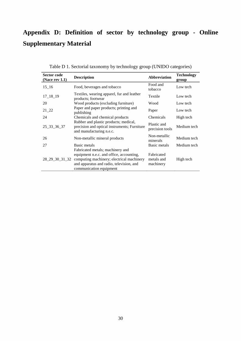
Table D 1. Sectorial taxonomy by technology group (UNIDO categories)

Sector code

(Nace rev 1.1) Description Abbreviation

Technology

group

15_16 Food, beverages and tobacco Food and

tobacco Low tech

17_18_19 Textiles, wearing apparel, fur and leather

products; footwear Textile Low tech

20 Wood products (excluding furniture) Wood Low tech

21_22 Paper and paper products; printing and

publishing Paper Low tech

24 Chemicals and chemical products Chemicals High tech

25_33_36_37

Rubber and plastic products; medical,

precision and optical instruments; Furniture

and manufacturing n.e.c.

Plastic and

precision tools Medium tech

26 Non-metallic mineral products Non-metallic

minerals Medium tech

27 Basic metals Basic metals Medium tech

28_29_30_31_32

Fabricated metals; machinery and

equipment n.e.c. and office, accounting,

computing machinery; electrical machinery

and apparatus and radio, television, and

communication equipment

Fabricated

metals and

machinery

High tech

Documents

Sustainable Development and Industrial Development ... · PDF file1 Sustainable Development and Industrial Development: Manufacturing Environmental Performance, Technology and Consumption/Production