Surface ozone in Yosemite National Park

ARTICLE IN PRESS

1352-2310/$ - se

doi:10.1016/j.at

�Correspondfax: +1925 376

E-mail add

John_D_Ray@

Atmospheric Environment 41 (2007) 6048–6062

www.elsevier.com/locate/atmosenv

Surface ozone in Yosemite National Park

Joel D. Burleya,�, John D. Rayb

aDepartment of Chemistry, Saint Mary’s College of California, Moraga, CA 94575-4527, USAbNational Park Service, Air Resources Division, P.O. Box 25287, Denver, CO 80225-0287, USA

Received 28 October 2006; received in revised form 10 February 2007; accepted 9 March 2007

Abstract

During the summers of 2003 and 2005, surface ozone concentrations were measured with portable ozone monitors at

multiple locations in and around Yosemite National Park. The goal of these measurements was to obtain a comprehensive

survey of ozone within Yosemite, which will help modelers predict and interpolate ozone concentrations in remote

locations and complex terrain. The data from the portable monitors were combined with concurrent and historical data

from two long-term monitoring stations located within the park (Turtleback Dome and Merced River) and previous

investigations with passive samplers. The results indicate that most sites in Yosemite experience roughly similar ozone

concentrations during well-mixed daytime periods, but dissimilar concentrations at night. Locations that are well exposed

to the free troposphere during evening hours tend to experience higher (and more variable) nocturnal ozone

concentrations, resulting in smaller diurnal variations and higher overall ozone exposures. Locations that are poorly

exposed to the free troposphere during nocturnal periods tend to experience very low evening ozone, yielding larger diurnal

variations and smaller overall exposures. Ozone concentrations are typically highest for the western and southern portions

of the park and lower for the eastern and northern regions, with substantial spatial and temporal variability. Back-

trajectory analyses suggest that air with high ozone concentrations at Yosemite often originates in the San Francisco Bay

Area and progresses through the Central California Valley before entering the park.

r 2007 Elsevier Ltd. All rights reserved.

Keywords: Ozone; Yosemite; Portable ozone monitor; HYSPLIT model

1. Introduction

First established as a national park in 1890,Yosemite is one of the most spectacular—andpopular—destinations within the national parksystem. Since 1987 the Air Resources Division ofthe National Park Service (NPS) has monitored

e front matter r 2007 Elsevier Ltd. All rights reserved

mosenv.2007.03.021

ing author. Tel.: +1 925 631 4839;

4027.

resses: [email protected] (J.D. Burley),

nps.gov (J.D. Ray).

surface ozone and other pollutants at a variety ofsampling locations within Yosemite in order tobetter understand how air pollution impacts parkresources (Air Quality in the National Parks, 2002).The deleterious effects of elevated ozone on SierraNevada forests have been thoroughly investigated;readers seeking a comprehensive review of this topicare directed to the excellent monograph edited byBytnerowicz et al. (2003). Most of the studies thathave been conducted so far have focused upon thewestern slope of the Sierra Nevada; relatively fewmeasurements of ozone have been made along the

.

www.elsevier.com/locate/atmosenv

dx.doi.org/10.1016/j.atmosenv.2007.03.021

mailto:[email protected]

mailto:[email protected]

ARTICLE IN PRESSJ.D. Burley, J.D. Ray / Atmospheric Environment 41 (2007) 6048–6062 6049

eastern slope, which lies along the eastern border ofYosemite. This lack of data has made it difficult formodelers to predict/interpolate ozone concentra-tions for these locations (Fraczek et al., 2003). Thegeneral problem of mapping/estimating ozonedistributions has also been complicated by the com-plex transport and mixing phenomena and variabletopography that are present throughout this region.Lee (2003) has specifically noted that more intensivesampling is needed in locations (e.g. Yosemite,Lassen Volcanic NP) where these conditions areprevalent.

Limited studies with low time resolution haveattempted to determine ozone concentrations withinYosemite based on simultaneous measurements atmultiple sites throughout the park (Bytnerowiczet al., 2003; Ray, 2001). In the study by Ray (2001),passive ozone samplers were deployed at 11 loca-tions spread across the park over 18-week summer-time periods to augment the concurrent measure-ments from the long-term monitoring station atTurtleback Dome. The results indicated that meanozone concentrations within the park increased withincreasing elevation at western sampling sites(approximate elevations of 1200–2000m above sealevel), but became variable at higher elevation sitesbetween 2000 and 3000m in the eastern part ofthe park.

The present report describes a series of surfaceozone measurements that were made in and aroundYosemite National Park during the summers of2003 and 2005. These measurements were combinedwith concurrent data from the Turtleback Domeand Merced River monitoring stations and pre-vious results from passive samplers to yield amore complete picture of surface ozone withinthe park.

2. Experimental methods and procedures

2.1. Portable ozone monitor, measurement protocols

Ambient ozone concentrations were measuredusing small, lightweight 2B Technologies Model 202ozone monitors. Two separate monitors wereutilized during the 2003 measurements, and a singlemonitor was used in 2005. In all cases, the samplinginlet consisted of a downward-facing 47mm dia-meter Teflon filter holder equipped with a 1–2 mmTeflon filter membrane. The filter holder wasconnected directly to the ozone monitor by a 2mlength of 6.35mm (0.25 in.) o.d. Teflon tubing. For

deployments at remote locations, the ozone monitorwas enclosed within a weatherproof plastic caseand the sampling inlet was covered by a plasticrain shield. Power for these remote deploy-ments was provided by a rechargeable 12-Vlead–acid battery with a capacity of 21Ah. Thisbattery was connected to a 20-W solar panelattached to the top of the plastic case. Ozoneconcentrations were measured at 10-s intervals, andthe data were recorded into internal monitormemory as 1-min averages. These 1-min valueswere later converted into hourly averages afterbeing downloaded from the ozone monitor. Thehourly data were then further averaged to obtainthe average diurnal cycle for each deploymentlocation.

2.2. Sampling locations

Measurements were conducted at a total of 12different locations in 2003, and five differentlocations in 2005. These sampling locations aresummarized in Table 1 and depicted in Fig. 1. Forsampling sites located near automobile traffic, themonitor was positioned at least 100m away fromthe closest road or parking lot in order to minimizeperturbations from vehicular exhaust. In all cases,the monitor was placed in an open clearing (i.e.away from nearby trees or bushes), with thesampling inlet positioned roughly 1.3m aboveground level.

2.3. Fixed-location monitoring stations

In addition to the data collected by the portableozone monitors, hourly ozone values were availablefrom two long-term monitoring stations locatedwithin the park. The Turtleback Dome stationwas fully operational in both 2003 and 2005, andthe Merced River station provided partial coveragein 2003 and full coverage in 2005. Both stationsfollowed Environmental Protection Agency (EPA)guidelines for sampling and analysis and utilizedthe Thermo Environmental Instruments Model49C photometric ozone analyzer to measure O3.The Turtleback Dome station also served as atest site where the performance of the portableozone monitors was verified under realistic samplingconditions. One of the co-located comparisonsconducted at the Turtleback Dome station in June2003 is discussed in detail below.

ARTICLE IN PRESS

Table 1

Sampling locations

Code Elevation

(m)

Latitude Longitude Start End Passive

sampler data

periods

2003 sites sampled by portable monitors

Turtleback Dome TD 1604 37.7133 �119.7060 18 June 25 June 2000–2003

Lee Vining Canyon LVC 2212 37.9371 �119.1382 27 June 2 July 2001

Tioga Pass #1 TP1 3037 37.9108 �119.2587 2 July 8 July 1998–2001

Crane Flat Lookout CFL 2022 37.7595 �119.8206 8 July 14 July 1999–2003

El Portal EP 603 37.6749 �119.8056 10 July 11 August

Tioga Road (T14) T14 2396 37.8397 �119.5904 14 July 21 July 1998–2001

Tuolumne Meadows #1 TM1 2623 37.8765 �119.3479 21 July 26 July 1998–2001

Siesta Lake SL 2446 37.8519 �119.6592 26 July 31 July 2000–2001

Merced River MR 1213 37.7431 �119.5940 1 August 5 August

Mirror Lake ML 1341 37.7518 �119.5522 7 August 11 August 2001

Tioga Pass #2 TP2 3021 37.9120 �119.2573 11 August 20 August

Tuolumne Meadows #2 TM2 2612 37.8757 �119.3763 11 August 20 August

2005 sites sampled by portable monitors

Turtleback Dome TD 1604 37.7133 �119.7060 17 July 20 July 2000–2003

Tuolumne Meadows #1 TM1 2623 37.8765 �119.3479 20 July 30 July 1998–2001

Dana Meadows DM 2869 37.8776 �119.2829 30 July 11 August

Lee Vining Canyon LVC 2212 37.9371 �119.1382 11 August 19 August 2001

Mono Lake MO 1957 37.9558 �119.0549 19 August 26 August

Sites sampled only by passive samplers

Camp Mather CM 1432 37.8886 �119.8411 1998 2003

Wawona Valley WV 1231 37.5402 �119.6524 1998 2003

Pohono (Valley A) PV 1210 37.7186 �119.6623 2000 2001

Taft Toe (Valley B) TT 1267 37.7208 �119.6235 2000 2001

Village (Valley C) YV 1224 37.7490 �119.5874 2000 2001

El Capitan Meadow ECM 1241 37.7259 �119.6383 2002 2003

Wood Yard WY 1272 37.7262 �119.6465 2002 2003

J.D. Burley, J.D. Ray / Atmospheric Environment 41 (2007) 6048–60626050

2.4. Sampling timelines

All of the portable ozone monitor data presentedin this report were collected between 18 June and 20August 2003 (day of year ¼ 169–232), or between17 July and 26 August 2005 (day of year ¼198–238). For most of the 2003 sampling period, itwas possible to obtain simultaneous ozone values atthree separate locations (Turtleback Dome stationplus one 2B monitor deployed to a remote site and asecond 2B monitor deployed to a site where ACpower was available). During those periods whenthe Merced River station was operational, thenumber of simultaneous ozone measurements in-creased to four. For the 2005 sampling period,simultaneous ozone values were available at threelocations: Turtleback Dome station, Merced Riverstation, and one 2B monitor deployed to a remotesite. In most cases, the sampling periods for theportable monitor deployments to remote locationsdo not overlap and are of different lengths.

2.5. Meteorological measurements at Tuolumne

Meadows and Tioga Pass

In order to better understand the transportmechanisms that can influence ozone concentrationsin alpine environments, the measurements per-formed in August 2003 at Tuolumne Meadowsand Tioga Pass were co-located with extensivemeteorological instrumentation (Clements et al.,2004; Clements, 2007). At Tuolumne Meadows(TM2), the ozone monitor was positioned near aDoppler sonic detection and ranging (SODAR)instrument and a portable meteorological tower.Concurrent measurements at Tioga Pass (TP2)employed an ozone monitor and a meteorologicaltower, but no SODAR. In both cases, the logisticalrequirements of the meteorological measurementsrequired that the sampling locations be moved fromtheir previous sites, so that while these newmeasurements correspond to the same approximateareas that had been sampled previously (TM1 and

ARTICLE IN PRESS

Fig. 1. Locations sampled by the portable ozone monitors. Sites sampled in 2003 are denoted by solid dots, while those sampled in 2005

are designated by larger open circles.

J.D. Burley, J.D. Ray / Atmospheric Environment 41 (2007) 6048–6062 6051

TP1), they do not correspond to the exact samepositions.

2.6. 2005 measurements at eastern sites

In the summer of 2005, measurements wereconducted along the easternmost portion of TiogaPass Road in order to obtain better coverage ofhigh-elevation sites extending eastward from Yose-mite into Inyo National Forest. Sampling sitesincluded two locations sampled in 2003 (TuolumneMeadows and Lee Vining Canyon) and two newlocations not previously sampled (Dana Meadowsand Mono Lake). The Dana Meadows site wasselected because of its location midway betweenTuolumne Meadows and Tioga Pass, and the MonoLake site was selected in order to determine if ozonetrends observed in the western portions of Yosemite

were being propagated eastward over Tioga Passand down into the Mono Lake basin.

2.7. Calibrations and comparisons involving the

portable ozone monitors

A variety of calibrations and comparisons wereperformed in order to verify the accuracy of theportable ozone monitors. Prior to field deployment,all of the 2B monitors used in this study werecalibrated in the laboratory against a transfer-standard Thermo Environmental Instruments Mod-el 49C photometric ozone analyzer. These initialtests typically spanned a concentration range of0–470 ppb and indicated that the portable monitorshad an overall precision of 74 ppb and an accuracyof 76%. Analogous post-deployment measure-ments after the completion of the summer sampling

ARTICLE IN PRESSJ.D. Burley, J.D. Ray / Atmospheric Environment 41 (2007) 6048–60626052

period indicated that the portable monitors hadretained a precision of 75 ppb and an accuracy of76%.

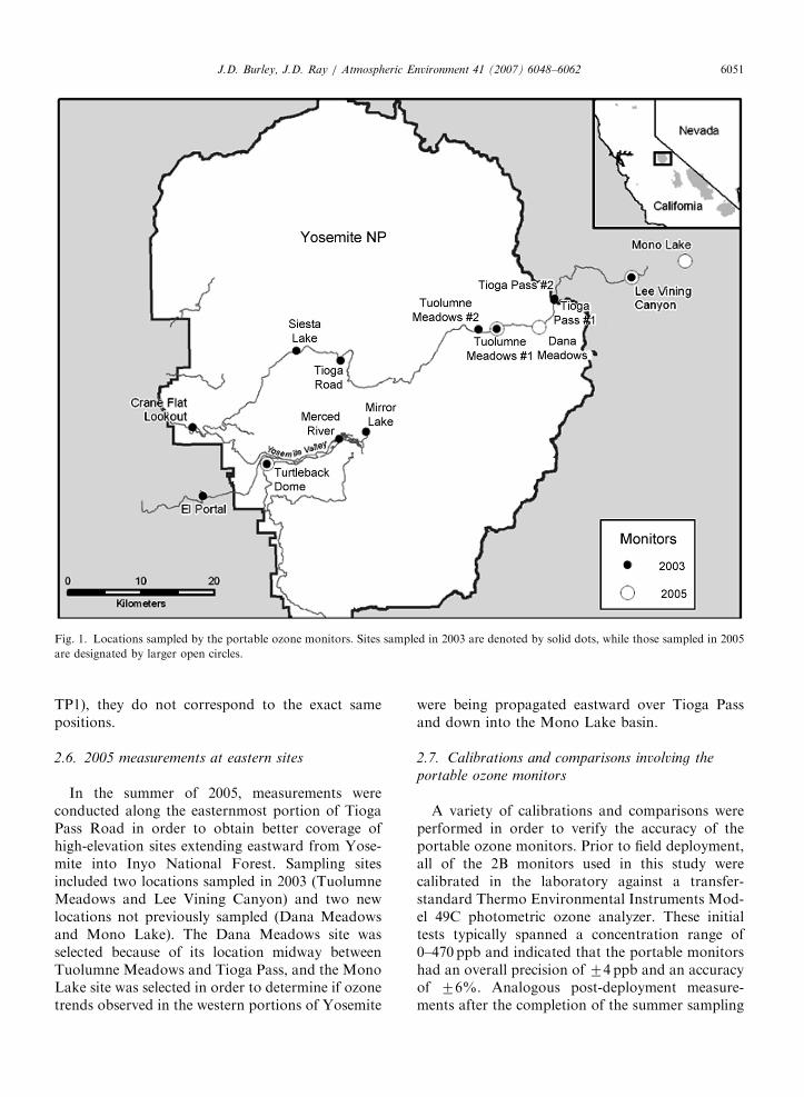
In addition to the laboratory calibrations, field testswere conducted at Turtleback Dome station. Thesetests demonstrated the reliability of the solar panel/rechargeable battery power source used for remotedeployments and allowed for direct comparisonsbetween the portable monitors and the station.Representative results from these tests are shown inFig. 2a. The hourly O3 values measured by the station

Fig. 2. (a) 2003 field test at Turtleback Dome station: time series com

measured by the portable ozone monitor and the thin line denotes the ho

station. (b) 2003 field test at Turtleback Dome station: scatter-plot anal

and nighttime data (18:00–8:00 PST) are designated by open triangle

daytime data; if the nighttime data are included in the linear regression

are, on average, 3.4ppb higher than those measured bythe portable monitor, and daytime deviations aretypically in the order of 0–3ppb. Significant deviationsare observed in the predawn hours for days 172–175,with the portable monitor yielding values that areconsistently low compared to the station. The probablecause for these predawn deviations is the different inletlocations employed by the two measurements. Asnoted above, the sampling inlet used by the portablemonitors was located approximately 1.3m aboveground level. In contrast, the inlet for the station was

parison. The thick line specifies the hourly ozone concentrations

urly concentrations recorded by the Turtleback Dome monitoring

ysis. Daytime data (9:00–17:00 PST) are indicated by solid circles

s. The linear regression shown on the graph corresponds to the

the R2 value decreases to 0.879.


mounted on a tower at a height of 10m. Localizedvariations in O3 concentration resulting from poormixing can typically become more pronounced duringevening hours (as opposed to the well-mixed daylighthours), so that the two different inlets can sampledifferent packets of air. A scatter-plot analysis of thetime series data from Fig. 2a, presented in Fig. 2b, isconsistent with this hypothesis. The scatter-plot in-dicates good agreement (R2

¼ 0.953, slope ¼ 0.948,y-intercept ¼ 0.357ppb) between the 2B monitor andthe station monitor for the well-mixed daylight hoursof 9:00–17:00 Pacific Standard Time (PST). If the datafor the evening and early morning hours (18:00–8:00PST) are added to the analysis so that the linearregression now includes all available data, a poorercorrelation (R2

¼ 0.879, slope ¼ 1.060, y-intercept ¼�6.88ppb) is obtained. Observations of inlet height-dependent sampling variations in predawn ozonevalues have also occurred during field-based compar-isons of the recently developed portable ozonemonitoring systems (POMS) to tower-based NPSmonitoring stations (Ray, 2006).

3. Results

3.1. 2003 measurements along Tioga Pass Road

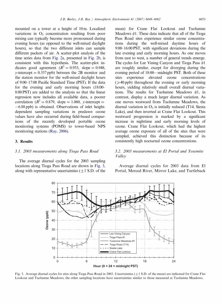
The average diurnal cycles for the 2003 samplinglocations along Tioga Pass Road are shown in Fig. 3,along with representative uncertainties (71 S.D. of the

0

10

20

30

40

50

60

70

80

0 6 1

Hour (0 = 24 =

Lee

Tiog

Tuol

Tiog

Sies

Cran

Ozo

ne (

pp

b)

Fig. 3. Average diurnal cycles for sites along Tioga Pass Road in 2003.

Lookout and Tuolumne Meadows; the other sampling locations have u

mean) for Crane Flat Lookout and TuolumneMeadows #1. These data indicate that all of the TiogaPass Road sites experience similar ozone concentra-tions during the well-mixed daytime hours of9:00–16:00PST, with significant deviations during thelate evening and early morning hours. As one movesfrom east to west, a number of general trends emerge.The cycles for Lee Vining Canyon and Tioga Pass #1are roughly similar, except for diverging during theevening period of 18:00—midnight PST. Both of thesesites experience elevated ozone concentrations(X40ppb) throughout the evening or early morninghours, yielding relatively small overall diurnal varia-tions. The results for Tuolumne Meadows #1, incontrast, display a much larger diurnal variation. Asone moves westward from Tuolumne Meadows, thediurnal variation in O3 is initially reduced (T14, SiestaLake), and then inverted at Crane Flat Lookout. Thiswestward progression is marked by a significantincrease in nighttime and early morning levels ofozone. Crane Flat Lookout, which had the highestaverage ozone exposure of all of the sites that weresampled, achieved this distinction because of itsconsistently high nocturnal ozone concentrations.

3.2. 2003 measurements at El Portal and Yosemite

Valley

Average diurnal cycles for 2003 data from ElPortal, Merced River, Mirror Lake, and Turtleback

2 18 24

midnight PST)

Vining Canyon

a Pass #1

umne Meadows #1

a Road (T14)

ta Lake

e Flat Lookout

Uncertainties (71 S.D. of the mean) are indicated for Crane Flat

ncertainties similar to those measured at Tuolumne Meadows.


Dome station are presented in Fig. 4, along with thecorresponding uncertainties. In contrast to Fig. 3,these sites show pronounced differences in themagnitudes of their afternoon maxima. El Portal,Merced River, Mirror Lake all display large diurnalvariations of 440 ppb, while at Turtleback Domethe diurnal variation is o30 ppb.

3.3. Additional 2003 measurements at Tuolumne

Meadows and Tioga Pass

The diurnal patterns resulting from the August2003 measurements with the co-located meteorologi-cal instrumentation (TM2 and TP2) are shown inFig. 5, along with the earlier data for TM1 and TP1.(The uncertainties for the TM2 and TP2 data—whichare slightly smaller than those observed for TM1 andTM2—have been omitted for purposes of legibility.)The reproducibility that is observed suggests that thediurnal cycles presented here are not significantlyperturbed by small changes in the sampling locations.

A preliminary analysis of the meteorological data(Clements et al., 2004) suggests that middle-of-the-night spikes in observed ozone concentrations resultfrom nocturnal mixing events in which air fromaloft (with elevated concentrations of O3) is mixeddownwards at higher elevations. This air is thenentrained into the surface layer, where it can betransported to lower elevations via nocturnal down-

0

10

20

30

40

50

60

70

80

0 6 1

Hour (0 = 24 =

El PMeMir

Tur

Ozo

ne (

pp

b)

Fig. 4. Average diurnal cycles for El Portal and Yosemite Valley sites

mean.

valley flows. A detailed analysis of the results isbeing prepared by Clements (2007).

3.4. 2005 measurements at eastern sites

The diurnal patterns for the 2005 measurementsare shown in Fig. 6. All of the eastern Tioga PassRoad sites display roughly similar behavior, with apronounced minimum near 6:00 followed by abroad maximum of approximately 45–50 ppb ex-tending between 10:00 and 16:00 PST. Comparisonof the data of Fig. 6 to analogous results from 2003indicates excellent reproducibility for TurtlebackDome station (Figs. 4 and 6) and good reproduci-bility for Tuolumne Meadows (Figs. 5 and 6).The 2005 measurements at Lee Vining Canyon,however, are dissimilar to those recorded in 2003(Fig. 3). The 2005 values are roughly 10–12 ppblower during daylight hours and up to 30 ppb lowerat night, primarily because the nighttime spikesfrequently observed at Lee Vining Canyon in the2003 hourly data are largely absent in 2005.

4. Analysis and discussion

4.1. Potential wildfire impacts

During the summers of 2003 and 2005, Yosemiteexperienced a number of wildfires (http://

2 18 24

midnight PST)

ortalrced Riverror Lake

tleback Dome Station

in 2003. The plotted uncertainties correspond to 71 S.D. of the

http://map.ngdc.noaa.gov/website/firedetects/viewer.htm

ARTICLE IN PRESS

0

10

20

30

40

50

60

70

0 6 12 18 24

Hour (0 = 24 = midnight PST)

Tuolumne Meadows #2

Tuolumne Meadows #1

Tioga Pass #2

Tioga Pass #1

Ozo

ne (

pp

b)

Fig. 5. Average diurnal cycles for deployments at Tuolumne Meadows and Tioga Pass in 2003. The TM1 and TP1 data are the same as

those presented in Fig. 3, and their plotted uncertainties correspond to 71 S.D. of the mean. The uncertainties for TM2 and TP2 (which

are not shown) are slightly smaller than those for TM1 and TP1.

0

10

20

30

40

50

60

70

80

0 6 12 18 24

Hour (0 = 24 = midnight PST)

Mono Lake

Lee Vining Canyon

Dana Meadows

Tuolumne Meadows #1

Turtleback Dome Station

Merced River Station

Ozo

ne (

pp

b)

Fig. 6. Average diurnal cycles for 2005 measurements. Representative uncertainties (71 S.D. of the mean) are indicated for Turtleback

Dome station and Tuolumne Meadows; the other sampling locations have uncertainties similar to those measured at Tuolumne Meadows.


map.ngdc.noaa.gov/website/firedetects/viewer.htm).The largest burn area was along the northwestboundary of the park and the burn areas alongTioga Road occurred in late August and Septemberafter the portable ozone measurements were com-pleted. While these wildfires could potentially haveperturbed the ozone results presented here (Hon-rath, 2004; McMeeking et al., 2005; APCD, 2003), a

preliminary analysis—based on fire records andparticulate matter data (PM 2.5 samplers andIMPROVE (Interagency Monitoring of ProtectedVisual Environments) monitors) collected inYosemite—does not suggest a strong influence.The fine particle data that would relate to wildfireswere not high during the ozone sampling periods.Likewise, the ozone record at Turtleback Dome was

http://map.ngdc.noaa.gov/website/firedetects/viewer.htm


consistent with values obtained over the last 10years. The agreement between the 2003 and 2005ozone data at three out of the four locationssampled in both years (Turtleback Dome, MercedRiver, Tuolumne Meadows) also supports thegeneral conclusion that the 2003 fires did notsignificantly perturb local ozone.

4.2. Diurnal patterns: general trends

The general features of the diurnal patternspresented in Figs. 3–6 most likely reflect thesurrounding topography and mixing dynamics,rather than local photochemical production of O3.According to this hypothesis, pronounced diurnalvariations with very low predawn ozone (such as isobserved at Tuolumne Meadows and Merced River)tend to be associated with flat topography thatpermits the recurring formation of a stable noctur-nal boundary layer near the surface. This boundarylayer typically prevents the downward mixing ofozone-rich air from the free troposphere duringevening hours, and allows for ozone near the surfaceto be removed by deposition and/or titration withNOx from nearby combustion sources. (Meteorolo-gical and NOx data from the Merced River stationsuggest that dry deposition, rather than titrationwith nitric oxide, is responsible for most of theozone loss that is observed at the Merced River site,but analogous data are not available for TuolumneMeadows.) Small diurnal variations are typicallyobserved when a sampling location lacks either (i)the flat topography and/or (ii) the local meteorolo-gical conditions needed to produce a stable noctur-nal boundary layer. Instead, these latter sitestypically experience turbulent mixing throughoutthe evening hours, and are well exposed to the freetroposphere.

4.3. Dual-peaked maxima in the diurnal plots

A number of sites sampled in 2003 and/or 2005display double-peaked maxima in their diurnalplots, with the observation of two distinct‘‘humps’’—one in the mid-morning and the otherin the early evening. Although most readilyobserved in the hourly data—which had to beomitted from the present report because of spaceconstraints—this phenomenon is clearly present inFig. 4 (Mirror Lake), Fig. 5 (Tuolumne Meadows#2 and Tioga Pass #2), and Fig. 6 (TuolumneMeadows #1). Similar behavior has been previously

studied in alpine environments by Loffler-Manget al. (1997), who attributed the first peak to themorning break-up of the nocturnal stable boundarylayer, with ozone-rich air mixing downwards fromabove. The second peak that arises a few hours latercorresponds to the horizontal transport of air viaup-valley winds.

The results from the two sites measured inYosemite Valley indicate that formation of dou-ble-peaked maxima may be highly dependent uponthe specific location of the sampling site. In thisinstance, the Mirror Lake data exhibit a pro-nounced double-humped appearance while thenearby Merced River data are consistently single-humped. The localized mixing dynamics at thesetwo valley sites may be very different (up-valley,base of cliffs for Mirror Lake versus down-valley,middle of meadow for Merced River), despite theirrelatively close proximity. The Mirror Lake site maybe seeing a wind rotator perpendicular to the up-valley flow that sets up as the sunlight warms thenearby canyon walls.

4.4. Small variation versus large variation sites

In general, the locations sampled in this reporttend to fall into two separate categories based uponthe magnitude of their diurnal variation. Smallvariation (or small delta) sites typically havepredawn ozone minima of �40 ppb or higher, withrelatively small diurnal variations of �25 ppb orless. These sites can experience frequent middle-of-the-night spikes in O3, which suggests that they arewell exposed to the free troposphere during eveninghours. Because these sites experience high levels ofnocturnal ozone, their average ozone exposuresover a 24-h period are typically 50 ppb or higher.The small variation sites include Turtleback Domestation, Tioga Pass, Crane Flat Lookout, T14, andSiesta Lake. Large variation (or large delta) sitestypically display predawn ozone minima of �25 ppbor lower, with diurnal variations of �40 ppb ormore. These sites usually experience diurnal pat-terns with relatively few nocturnal ozone spikes, andthey are not well exposed to the free troposphereduring the evening. Because these locations experi-ence very low levels of nocturnal ozone, theiraverage ozone exposures over a 24-h period aretypically below 50 ppb. The large variation sitesinclude El Portal, Tuolumne Meadows, DanaMeadows, Merced River station, Mirror Lake,and Mono Lake.


The Lee Vining Canyon site—which was mea-sured by the portable monitor in both 2003 and2005—may be unlike the other locations in that itdoes not consistently demonstrate ‘‘small-delta’’ or‘‘large-delta’’ behavior. The lack of reproducibilityin the 2003 versus 2005 results might indicate thatthis site is topographically ‘‘flat’’ enough toexperience stable nocturnal boundary layers whenallowed by local meteorological conditions (2005data) while at the same time exposed enough toexperience recurring downward mixing events dur-ing periods of greater nocturnal turbulence (2003data).

Similar variations in the magnitude of the diurnalvariability have been observed in previous studies ofSierra Nevada ozone. Van Ooy and Carroll (1994)observed significant differences in the strength ofthe diurnal pattern at six remote sites along thewestern slope of the Sierra Nevada. They hypothe-sized that local topographical characteristics andtheir effect on the local transport of polluted airwere the predominant factors in determining thestrength of the diurnal variation, rather than thelinear distance of the site from urban sources. Thepresent results support this hypothesis and suggestthat it can be extended to sites at higher elevationsthan those measured by Van Ooy and Carroll(1994).

4.5. Comparisons of scaled results to passive sampler

data

In order to quantitatively compare ozone trendsacross different sampling locations and removetemporal variability, the raw hourly data weremultiplied by scaling factors that are specific tothe day on which the data were collected

Daily scaling factor

¼½TDstation average for 1 June to 31August�

½TD station average for that day�.

ð1Þ

These scaling factors assume that TurtlebackDome station can serve as a reliable frame ofreference for the entire park and that regional trendsin ozone concentration will be seen more or lessuniformly throughout the park. No adjustments aremade for potential year-to-year variations betweenthe 2003 and the 2005 data, and the scaling factorsapplied to the 2003 results are therefore completelyindependent of those applied to the 2005 data. (The

2003 ozone concentrations are somewhat higherthan those collected in 2005, so that the numeratorof Eq. (1) decreases from 60.6 ppb in 2003 to56.7 ppb in 2005.)

On days when regional ozone concentrations arehigh, the daily scaling factor is o1, while on dayswhen regional ozone values are low the scalingfactor is 41. As a result, sites that were sampledduring periods of high regional ozone have theirozone values scaled downwards while those sampledduring cleaner periods have their ozone valuesadjusted upwards. After the scaling factors areapplied to the hourly data for a given site, the scaledhourly data are averaged to yield a single ozonevalue for that location. To prevent the results frombeing skewed by inconsistent sampling periods, onlycomplete, contiguous 24-h blocks of data areincluded in the calculation of the overall average.This scaling and averaging process makes it possibleto estimate a single average value for a 3-monthseasonal period (June–July–August) from a limited-duration time series of hourly data. It also facilitatesdirect comparisons to passive sampler data fromprevious years, which have been archived as weeklyvalues and can therefore be converted directly into3-month seasonal averages.

4.6. Spatial trends

The ozone concentrations resulting from thescaling and averaging process outlined above arepresented in Figs. 7–9, along with June–July–August seasonal average values for passive samplerdata from 1998 through 2003. Most locations haveresults from both the portable monitor measure-ments and the passive samplers, but seven sites haveonly passive sampler data (Table 1).

A number of general trends are apparent in thedata of Figs. 7–9. The portable ozone monitors andthe passive ozone samplers (Ray, 2001) yield similarresults, as indicated by the small range of ozonevalues at each site. Larger scatter is observed formeasurements within Yosemite Valley and at LeeVining Canyon. When the data for the smallvariation and large variation sites are examinedindependently, two distinct bands emerge, assuggested by the trend lines plotted in Fig. 7. Theselinear regressions are based only on the 2003 and2005 data from the continuous samplers andexclude the results from the Yosemite Valley (toomuch site-to-site variability within the valley) andLee Vining Canyon (inconsistent behavior between

ARTICLE IN PRESS

y = -0.0040x + 66.0371

R2 = 0.3982

y = -0.0048x + 47.4040

R2 = 0.7305

20

30

40

50

60

70

500 1000 1500 2000 2500 3000

Elevation (m)

small delta sites

large delta sites

Merced River, Mirror Lake

Lee Vining Canyon

passive samplers 1998






Linear (small delta sites)

Linear (large delta sites)

EP

TM

TP

TD

CFL

LVC

T14, SL

Valley Sites

and WV

CM

MO

DM

Avera

ge O

zo

ne (

pp

b)

Fig. 7. Elevation dependence of scaled average ozone values. Trend lines for the small variation and large variation sites are based upon

continuous measurements from 2003 and 2005 (excluding Yosemite Valley and Lee Vining Canyon) and do not include any passive

sampler data.

y = -14.46x - 1672.23

R2 = 0.65

y = -8.80x - 1013.72

R2 = 0.20

20

30

40

50

60

70

-120.0 -119.8 -119.6 -119.4 -119.2 -119.0

Longitude (degrees)

TDCFL

T14

TP

LVC

TM

EP

CM

Valley Sitesand WV

MO

SL

DM

Avera

ge O

zo

ne (

pp

b)

Fig. 8. Longitudinal dependence of scaled average ozone values. Trend lines for the small variation and large variation sites are based

upon continuous measurements from 2003 and 2005 (excluding Yosemite Valley and Lee Vining Canyon) and do not include any passive

sampler data. The data symbols are the same as those used in Fig. 7.


2003 and 2005). Both the small variation and thelarge variation sites experience average ozoneexposures that decrease with increasing elevation,and the observed slopes are roughly similar for thetwo different types of locations. (It should be noted,however, that the small-delta and large-delta slopesare not co-linear—the regressions shown inFigs. 7–9 have low R2 values.) A longitudinal

analysis (Fig. 8) also separates into distinct bandsfor the small variation and large variation sites, withaverage ozone decreasing as one moves from west toeast. A latitudinal analysis (Fig. 9) shows a similarpattern, with ozone concentrations decreasing asone moves from south to north. The overall picturethat emerges is that average ozone exposures withinthe park generally decrease as one moves from low

ARTICLE IN PRESS

y = -34.67x + 1368.34

R2 = 0.52

y = -30.35x + 1185.67

R2 = 0.36

20

30

40

50

60

70

37.5 37.6 37.6 37.7 37.7 37.8 37.8 37.9 37.9 38.0 38.0

Latitude (degrees)

WV

TD

CFL

T14, SL

TP

LVC

TM, DM

EP CM

Valley Sites

MO

Avera

ge O

zo

ne (

pp

b)

Fig. 9. Latitudinal dependence of scaled average ozone values. Trend lines for the small variation and large variation sites are based upon

continuous measurements from 2003 and 2005 (excluding Yosemite Valley and Lee Vining Canyon) and do not include any passive

sampler data. The data symbols are the same as those used in Fig. 7.


elevations in the south and west to higher elevationsin the north and east, but with substantial spatialand temporal variability.

4.7. Back-trajectory calculations

In order to understand the transport dynamicsthat bring polluted air into Yosemite, the HybridSingle-Particle Lagrangian Integrated Trajectory(HYSPLIT) model from the Air Resources Labora-tory of the National Oceanic and AtmosphericAdministration was used to perform a series ofback-trajectory calculations (Draxler and Rolph,2003; Rolph, 2003). Calculations were conductedfor days between 1 June and 31 August 2003, whenthe maximum 1-h ozone concentration measured atTurtleback Dome station exceeded 80 ppb. In allcases, the back-trajectories were configured with aninitial elevation of 100m above ground level, anarrival time at Turtleback Dome of 14:00 PST, andan overall length of 48 h. The Eta Data AssimilationSystem (EDAS) 80 km data set was used to providethe archived meteorological data required for modelinput (Draxler and Rolph, 2003).

The results from the back-trajectory calculationsindicate that most of the air that was transportedinto Yosemite originated in the San Francisco BayArea before passing through the Central Valley andthen into the park. In a typical trajectory, such asthe one shown in Fig. 10, an onshore flow occurs in

Marin County and then proceeds eastward throughthe Carquinez Strait and up into the Delta beforeturning to the south and entering the Central Valley.(In some cases, the onshore flow can originate southof San Francisco and travel inland over theAltamont Pass before turning southward.) Aftertraveling down the Central Valley, the air parcelthen turns to the east to ascend through the SierraNevada foothills and make a final approach intoYosemite. Typical transit times from the Bay Areato Yosemite are on the order of 24–36 h. Thegeneral pattern displayed in Fig. 10 is fullyconsistent with previous investigations of surface-level meteorology (California Air Resources Board,2001).

While the back-trajectory pictured in Fig. 10represents the most common scenario for pollutanttransport into Yosemite, approaches from otherdirections are also frequently observed. It is there-fore useful to calculate the relative probabilities forall possible approaches into the park. Fig. 11presents the weighted source contribution plot(Ashbaugh et al., 1985; Gebhart et al., 2006) forthe summer 2003 high ozone back-trajectories atTurtleback Dome station. In this representation, theshade of a given grid element indicates the relativesource contribution from back-trajectories thatpassed through that particular region before arriv-ing at Turtleback Dome station. In addition to aheavy source contribution from the San Francisco

ARTICLE IN PRESS

Fig. 10. Air mass back-trajectory (100m AGL) for 14 August 2003. Arrival time at Turtleback Dome station (latitude ¼ 37.7131;

longitude ¼ �119.7061) is 14:00 PST (22:00 UTC). Trajectory duration ¼ 48 h.

Fig. 11. Source contribution plot based on daily back-trajectory calculations for June–August 2003. Back-trajectories are restricted to

days with ozone of 80 ppb or greater. The arrival time at Turtleback Dome station is 14:00 PST (22:00 UTC), the trajectory height is 100m

AGL, and the trajectory duration is 48 h. Darker grid rectangles have a higher fraction of trajectories that traverse that area.



Bay Area, Fig. 11 indicates a secondary contribu-tion from eastern Nevada. A longer period was alsoinvestigated for hourly ozone maxima 480 ppb atTurtleback Dome during summers between 1999and 2004. The eastern Nevada/Reno region wasindicated as a source area even more strongly in thisanalysis.

4.8. Emission sources

Although the HYSPLIT back-trajectory calcula-tions indicate that air transported into Yosemite onhigh ozone days usually originates in the Bay Area,most of the pollution entering the park is believed toresult from emissions that occur downwind from theBay Area, as the trajectories pass through theCentral Valley and Sierra Nevada foothills. Dreyfuset al. (2002) and Dillon et al. (2002) examined thetransport and chemical evolution of pollutantsemitted in the Sacramento urban plume. Theirresults indicated that high ozone at the BlodgettForest Research Station (located northwest ofSacramento along the western slope of the SierraNevada) is caused by anthropogenic emissions inthe Central Valley and/or biogenic emissions in theSierra Nevada foothills, and that the latter can playa significant role (Dreyfus et al., 2002). Jacobsen(2001) used a global-through urban-scale nested airpollution/weather forecast model to estimate thesources of surface ozone measured at numerouslocations throughout northern and central Califor-nia, including Yosemite. His calculations indicatedthat for typical summertime maxima, roughly 54%of the ozone in Yosemite was from anthropogenicsources, 4% was biogenic-hydrocarbon in origin,and the rest was background. The present results donot address the relative magnitudes of the differentupwind emission sources that are expected to beimportant for Yosemite, but they do support thegeneral hypothesis that regional-scale transport ofpollutants into the park greatly exceeds local, park-based emissions.

5. Conclusion

Most sites in and around Yosemite experienceroughly similar ozone concentrations during well-mixed daytime periods, but dissimilar concentra-tions at night. Locations that are well exposed to thefree troposphere during evening hours tend toexperience higher (and more variable) nocturnalozone concentrations, resulting in smaller diurnal

variations and higher overall ozone exposures.Locations that are poorly exposed to the freetroposphere during nocturnal periods tend toexperience very low evening ozone, yielding largerdiurnal variations and smaller overall exposures.The present data suggest that modelers need toexplicitly include the local topography and trans-port dynamics when attempting interpolations/assessments for remote locations and complexterrain.

Acknowledgments

Financial support for this project was providedby the Faculty Alumni Fellowship Fund and theFaculty Development Fund at Saint Mary’s College(SMC), and by the Air Resources Division of theNational Park Service. SMC students ChristinaEstill and Jason McLean assisted with data collec-tion and analysis in 2003. Essential logisticalsupport at Yosemite National Park was providedby Katy Warner, Kyle Kline, and Lee Tarnay, whileLarry Ford provided support for measurements inInyo National Forest. Debbie Miller and DrewBingham at the NPS Air Resources Divisionassisted in the map and back-trajectory graphics.The authors gratefully acknowledge the NOAA AirResources Laboratory (ARL) for the provision ofthe HYSPLIT transport and dispersion model usedin this publication. Thanks are also due to CraigClements for sharing his SODAR and meteorologi-cal data.

References

Air Pollution Control Division (APCD), 2003. Colorado

Department of Public Health and Environment, Denver,

CO /http://apcd.state.co.us/psi/smkozone.htmlS.

Air Quality in the National Parks, 2002. Air Resources Division

Report, National Park Service, Denver, CO /http://

www2.nature.nps.gov/air/pubs/aqnps.htmS.

Ashbaugh, L.L., Malm, W.C., Sadeh, W.Z., 1985. A residence

time probability analysis of sulfur concentrations at Grand

Canyon National Park. Atmospheric Environment 19,

1263–1270.

Bytnerowicz, A., Arbaugh, M.J., Alonso, R. (Eds.), 2003. Ozone

Air Pollution in the Sierra Nevada: Distribution and Effects

on Forests. Elsevier, Amsterdam.

California Air Resources Board, 2001. Ozone Transport: 2001

Review. California Environmental Protection Agency, Sacra-

mento, CA.

Clements, C.B., 2007, in preparation.

Clements, C.B., Zhong, S., Kim, S.B., Kim, S., Burley, J.D.,

2004. High-altitude ozone concentrations in Yosemite

http://apcd.state.co.us/psi/smkozone.html

http://www2.nature.nps.gov/air/pubs/aqnps.htm

http://www2.nature.nps.gov/air/pubs/aqnps.htm


National Park, Sierra Nevada. In: Proceedings of the 16th

Conference on Air Pollution Meteorology, American Meteor-

ological Society. Vancouver, BC, 22–27 August 2004.

Dillon, M.B., Lamanna, M.S., Schade, G.W., Goldstein, A.H.,

Cohen, R.C., 2002. Chemical evolution of the Sacramento

urban plume: transport and oxidation. Journal of Geophysi-

cal Research 107 (D5), 4045–4059.

Draxler, R.R., Rolph, G.D., 2003. HYSPLIT (Hybrid Single-

Particle Lagrangian Integrated Trajectory) Model access via

NOAA ARL READY Website /http://www.arl.noaa.gov/

ready/hysplit4.htmlS. NOAA Air Resources Laboratory,

Silver Spring, MD.

Dreyfus, G.B., Schade, G.W., Goldstein, A.H., 2002. Observa-

tional constraints on the contribution of isoprene oxidation to

ozone production on the western slope of the Sierra Nevada,

California. Journal of Geophysical Research 107 (D19),

4365–4381.

Fraczek, W., Bytnerowicz, A., Arbaugh, M.J., 2003. Use of

geostatistics to estimate surface ozone patterns. In: Bytner-

owicz, A., Arbaugh, M.J., Alonso, R. (Eds.), Ozone Air

Pollution in the Sierra Nevada: Distribution and Effects on

Forests. Elsevier, Amsterdam, pp. 215–247.

Gebhart, K.A., Schichtel, B.A., Barna, M.G., Malm, W.C., 2006.

Quantitative back-trajectory apportionment of sources of

particulate sulfate at Big Bend National Park, TX. Atmo-

spheric Environment 40, 2823–2834.

Honrath, R.E., 2004. Regional and hemispheric impacts of

anthropogenic and biomass burning emissions on summer-

time CO and O3 in the North Atlantic lower free troposphere.

Journal of Geophysical Research 109 (D24).

Jacobsen, M.Z., 2001. GATOR-GCMM 2. A study of daytime

and nighttime ozone layers aloft, ozone in national parks, and

weather during the SARMAP field campaign. Journal of

Geophysical Research 106 (D6), 5403–5420.

Lee, E.H., 2003. Use of auxiliary data for spatial interpolation of

surface ozone patterns. In: Bytnerowicz, A., Arbaugh, M.J.,

Alonso, R. (Eds.), Ozone Air Pollution in the Sierra Nevada:

Distribution and Effects on Forests. Elsevier, Amsterdam,

pp. 165–194.

Loffler-Mang, M., Kossmann, M., Vogtlin, R., Fiedler, F., 1997.

Valley wind systems and their influence on nocturnal ozone

concentrations. Contributions to Atmospheric Physics 70, 1–14.

McMeeking, G.R., Kreidenweis, S.M., Carrico, C.M., Lee, T.,

Collet Jr., J.L., Malm, W.C., 2005. Observations of smoke

influenced aerosol during the Yosemite Aerosol Characteriza-

tion Study: size distributions and chemical composition.

Journal of Geophysical Research 110 (D18).

Ray, J.D., 2001. Spatial distribution of tropospheric ozone in

National Parks of California: interpretation of passive-

sampler data. The Scientific World 1, 483–497.

Ray, J.D., 2006. Portable Ozone Systems (POMS). Air Resources

Division, National Park Service /http://www2.nature.

nps.gov/air/studies/portO3.cfmS.

Rolph, G.D., 2003. Real-time Environmental Applications and

Display system (READY) Website /http://www.arl.noaa.

gov/ready/hysplit4.htmlS. NOAA Air Resources Laboratory,

Silver Spring, MD.

Van Ooy, D.J., Carroll, J.J., 1994. The spatial variation of ozone

climatology on the western slope of the Sierra Nevada.

Atmospheric Environment 29, 1319–1330.

http://www.arl.noaa.gov/ready/hysplit4.html


http://www2.nature.nps.gov/air/studies/portO3.cfm

http://www2.nature.nps.gov/air/studies/portO3.cfm



Documents

Surface ozone in Yosemite National Park