Supply Chain Resilience:

Should Policy Promote Diversification or Reshoring?∗

Gene M. Grossman

Princeton University

Elhanan Helpman

Harvard University

Hugo Lhuillier

Princeton University

September 27, 2021

Abstract

Supply chain disruptions, which have become commonplace, are often associated with glob-

alization and trade. Little is known about optimal policy in the face of insecure supply chains.

Should governments promote resilience by subsidizing backup sources of input supply? Should

they encourage firms to source from closer and presumably safer domestic suppliers? We ad-

dress these questions in a very simple model of production with a single critical input and

with exogenous risks of relationship-specific and country-wide supply disturbances. We follow

Matsuyama and Ushchev (2020) in positing a class of preferences that are homothetic with a

single aggregator and that obey Marshall’s Second Law of Demand. The familiar case of CES

preferences is a member of the class, but it imposes restrictions that are important for policy

conclusions.We find that, in the CES case, a subsidy for diversification achieves the constrained

social optimum and dominates a policy that promotes reshoring or offshoring. When the de-

mand elasticity rises with price, two policy instruments generally are needed to achieve efficient

supply chains, private investments in resilience may be socially excessive, and policy that alter

incentives to invest at home versus abroad may achieve greater welfare than ones that encourage

or discourage diversification.

Keywords: global supply chains, global value chains, input sourcing, resilience.

JEL Classification: F13, H21, F12

∗We are grateful to Maxim Alekseev and Alejandro Sabal for excellent research assistance.

1 Introduction

The United States needs resilient, diverse, and secure supply chains to ensure our economic

prosperity and national security. Pandemics and other biological threats, cyber-attacks, climate

shocks and extreme weather events, terrorist attacks, geopolitical and economic competition,

and other conditions can reduce critical manufacturing capacity and the availability and integrity

of critical goods, products, and services. Resilient American supply chains will revitalize and

rebuild domestic manufacturing capacity, maintain America’s competitive edge in research and

development, and create well-paying jobs.

Joseph R. Biden, Jr., Executive Order on America’s Supply Chains, February 24, 2021

Supply chain disruptions have become the new normal. The Great East Japan Earthquake

of 2011, and the massive tsunami that it triggered, brought such occurrences to the attention of

economists. Since then, hardly a month passes without news of a fresh disturbance. The pace of

disruptions has quickened with the advent of the COVID-19 pandemic, and now we hear regularly

of supply chain breakdowns in industries as disparate as automobiles, dishwashers, plastics, copper

wire, lumber, pork, and toilet paper.

Disruptions have a myriad of causes. They result from natural disasters, geopolitical disputes,

transportation failures, cyber-attacks, fires, power outages, labor shortages, human error and, of

course, pandemics. McKinsey Global Institute (2020), which recently conducted a series of inter-

views with supply chain experts, reports that disruptions lasting one to two weeks happen to a

given company on average every second year, while those lasting one to two months occur every

3.7 years. They find that an industry’s exposure to shocks reflects its geographic footprint and its

production technology, with greatest exposure in medical devices, wooden products, and fabricated

metal products and least exposure in communications equipment, apparel, and petroleum products

(see Exhibit E2 on p.6). The disruptions impose significant costs, presenting firms with expected

losses of between 24% of a year’s earnings before interest, taxes, depreciation and amortization

(EBITDA) in pharmaceuticals to 67% in aerospace, over a ten-year period. Across the thirteen

industries that McKinsey examined, the expected losses per decade amounted to about 42% of

annual EBITDA (see Exhibit E5 on p.12).

Carvalho et al. (2021) provide a more rigorous quantitative assessment of one major disruption,

namely the aforementioned Japanese earthquake of 2011. They focus on the role of input-output

linkages as a mechanism for propagation and amplification of shocks, exploiting the exogenous

nature of the event, its enormous impact on a subset of firms, and its localized incidence. Beyond

the direct effects, they find that firms whose suppliers were hit hard by the natural disaster suffered

substantial sale losses compared to others, as did firms whose downstream customers were hit. Using

a calibrated general-equilibrium model of production networks, they conclude that the disaster

imposed a 0.47 percentage point reduction in Japan’s aggregate real GDP growth.

Many commentators associate the increasing frequency and severity of supply chain disruptions

1

with the recent history of rapid globalization.1 This perceived connection, in turn, has sparked soul

searching amongst policy makers and a call to action in the broader public. If costly shocks reflect

concentration of input supplies in a few regions or countries, wouldn’t it be sensible for governments

to encourage firms to diversify their sourcing? And if distance from suppliers intensifies the risk of

disruption, wouldn’t it be better to bring some parts of the supply chains back home? The preamble

to President Biden’s February 24th 2021 Executive Order suggests that “diverse and secure supply

chains” are a prerequisite for economic prosperity and that “resilient American supply chains” will

rest on “rebuil[t] domestic manufacturing capacity [emphasis added].”

Little is known about the efficacy of policies aimed at supply chain management in an environ-

ment with recurring disturbances. Disruptions generate input shortages that can give rise to price

spikes or even outright unavailability of downstream products. Consumers suffer from their ham-

pered ability to purchase the products they covet. To the extent that households forfeit consumer

surplus in the face of supply chain disruptions, governments may have reason to enact policies that

curtail their occurrence.

But the policy calculus is not so simple. Production impediments impact not only consumers’

surplus, but also firms’ bottom lines. The question for governments is not whether shortages

adversely affect households, but whether firms’ private incentives to avoid such shortages fall short

of (or exceed) what is socially desirable. Firms may have inadequate incentives to invest in supply-

chain resilience, because they do not capture all of the surplus from offering their products to the

market. But they may also have an excessive taste for resilience arising from their desire to be in

a position to capitalize on extraordinary profit opportunities when their rivals are hit with supply

problems of their own.

In this paper, we propose a bare-bones framework that can aid with evaluating policy that

influences the organization of supply chains. Our framework puts supply shortages front and

center. We abstract from all complexity in the production process by assuming that each firm

manufactures a differentiated variety of some good using a single, critical input. If the supply chain

operates smoothly, the firm produces one unit of its variety from one unit of the customized input.

But exogenous shocks may disrupt supplier-buyer relationships. We allow for two types of shocks,

those that idiosyncratically sever a single chain and those that impede all supply from a particular

source country. Each firm may establish a relationship with a potential supplier in a low-cost but

riskier foreign country, in a higher-cost but safer home location, or in both. To form a relationship

with some supplier, the firm incurs a fixed cost. A firm can invest in resilience by avoiding the

riskier foreign supply or, even more so, by diversifying its supply base by establishing relationships

in both countries. In equilibrium, there are four possible states of the aggregate economy: supply

chains may be operative only with home suppliers, only with foreign suppliers, with neither, or with

both. The fixed mass of final producers chooses among four strategies: invest in a single supply

relationship domestically, invest in a single relationship abroad, diversify, or exit. Their collective

choices determine equilibrium prices, equilibrium variety, profits, surplus and (with fiscal policies

1See, for example, Shih (2020a, 2020b) and Iakovou and White III (2020).

2

in place) government revenues in each state of the world. Using these state-contingent aggregate

outcomes, we can calculate expected welfare under different policy regimes.

We consider three alternative policy options, separately and in combination. The government

might promote or discourage diversification, which we operationalize as a subsidy or tax on a firm’s

formation of a second supply relationship. Also, the government might promote or discourage

“reshoring” with a subsidy or tax for establishing a supply relationship specifically in the home

country. Finally, the government might promote or discourage offshoring with a subsidy or tax

for establishing a supply relationship abroad. These policies alter the availability of products in

the various states of the world. We examine which types of policies increase welfare and how the

optimal second and third-best policies compare in their efficacy. In order to elucidate the role

that policy plays in each environment, we sometimes allow for an optimal consumption subsidy

alongside the policies that directly affect the incentives for supply-chain organization. It is well-

known that markup pricing generates undersupply in settings of imperfect competition (see, for

example, Dhingra and Morrow, 2019, and Campolmi et al., 2021), so considering supply-chain policy

together with consumption subsidies clarifies whether the former just substitutes (imperfectly) for

the latter, or whether it can play some additional role in promoting continued availability in the

face of adverse supply shocks.

Inasmuch as the social cost of supply-chain disruptions stems from loss of consumer surplus, the

form of consumer preferences plays a crucial role in any policy analysis. It has become commonplace

to use CES preferences in trade models with endogenous availability of differentiated products, but

the very special properties of these preferences have been recognized since the seminal work by

Dixit and Stiglitz (1977). The market undersupplies variety, because firms do not capture all of the

surplus from their investments. But it oversupplies variety, because some of a firm’s profits come

at the expense of rival firms. In many contexts with CES preferences, these opposing forces happen

exactly to offset one another. These considerations apply as much to investments in “resilience” as

they do to investments in entry, so it is important for understanding the dictates of optimal policy

addressing the organization of supply chains to allow for more flexible forms of demand. To this

end, we follow Matsuyama and Ushchev (2020) in adopting a broader class of preferences that are

Homothetic with a Single Aggregator (HSA). With HSA preferences, the demand for any variety

per unit of income depends on the price of the variety relative to a (common) aggregator of all

prices. The CES utility function is a member of this class wherein the ideal price index plays a

dual role of inversely measuring welfare and capturing the competitive pressure from rival varieties.

More generally, HSA preferences allow the demand elasticity for a variety to vary along the demand

curve and the aggregator that enters demand to differ from the one that measures welfare.

Needless to say, there are many ways that our analysis could be enriched beyond allowing

for a broader class of demands than CES. For example, we could introduce a richer technology

with potential substitution between manufactured inputs and primary factors of production. We

could entertain more complex supply chains, with multiple inputs and with a sequencing of them

such that some inputs enter the production process upstream from others. We could allow for

3

dynamics, which would render inventories an additional tool for firms to invest in resilience and

give governments additional policy instruments such as stockpiling supplies or allowing accelerated

depreciation of inventory costs. We could introduce political-economy considerations that might

drive a wedge between the parameters that capture the risk aversion of managers versus that of

policy makers. We see all of these potential extensions as worthwhile and germane to the ultimate

policy assessment. Our simpler setting suggests a way to pose the question and our analysis provides

a “proof of concept.”

Our paper fits into an earlier literature on trade disruptions in a neoclassical setting. Much

of this previous work addressed optimal policy responses to potential trade embargoes. Mayer

(1977) showed that production subsidies are an optimal response to threats of trade interruption

in the presence of costly adjustment. Bhagwati and Srinivasan (1976) made the likelihood of a

disruption a function of the volume of trade and elucidated an efficiency role for tariffs to give

agents an incentive to internalize the externality arising from their effect on the probability of a

trade restriction. Arad and Hillman (1979) extended these earlier papers to allow for learning-by-

doing in the production of a good that might later be subject to an embargo. Bergstrom et al.

(1985) developed an infinite-horizon model to study the potential role of inventories to mitigate

the threat of embargo. Perhaps the most sophisticated of these early studies was that by Cheng

(1989), who considered recurrent embargo threats as a two-state stationary Markov process that

plays out with constraints on the speed of intersectoral reallocation.

The main difference between our work and this earlier literature stems from our treatment of

the endogenous availability of differentiated products. With perfect competition and homogeneous

goods, aggregate quantities matter for welfare but the availability of a particular firm’s offering

does not. If a disruption causes some import good to be unavailable, there is no harm to consumers

beyond the higher price of the domestic (perfect) substitutes. The number of viable producers

plays no role in neoclassical welfare analysis and is not even well defined. Of course, higher sticker

prices play a role also in a world with differentiated products, but there is also a direct harm to

consumers from a particular variety not being available for purchase. For this reason, we believe

that endogenous determination of the set of available products should feature prominently when

evaluating policy toward supply-chain security.

The remainder of the paper is organized as follows. In Section 2 we develop a very simple

model of risky supply chains in which final goods are produced with a single, critical input that

may be subject to relationship-specific and country-wide supply shocks. Section 3 builds intuition

by examining the case in which the home and foreign countries offer similar costs and pose similar

risks. In this symmetric case, we are able to derive a number of analytical results concerning the

relative ranking of policies that affect the incentives for diversification versus ones that encourage

or discourage relationships in one country or the other. We also show that it is optimal for the

government to encourage greater supply-chain resilience when demand elasticities are constant, but

not necessarily so if demand for a brand becomes more elastic as its price rises. In Section 4, we

address the more interesting but more difficult case in which suppliers in the home country are safer

4

but more expensive than those abroad. Here too, the case of CES preferences admits an analytical

approach and we find again that the competitive equilibrium provides too little resilience and

that diversification policies dominate others that affect the incentives firms have to source in one

country or the other. For more general HSA preferences we resort to numerical methods. Although

a range outcomes is theoretically possible, the dominance of diversification policies over reshoring

and offshoring policies seems reasonably robust when the elasticity of demand for differentiated

products is sufficiently above one.

2 A Simple Model of Risky Supply Chains

2.1 Supply Relationships

The home economy produces a homogeneous, numeraire good and potentially a unit measure of

nontraded differentiated final products. Firm ω in the latter industry converts a single, customized

critical input into the final good ω using the linear production technology,

x (ω) = m (ω) ,

where x (ω) is output of good ω and m (ω) is the quantity of the customized input. If the firm has

established a supplier relationship in country i and if that supply chain is operative, then the firm

can procure the customized inputs at unit cost qi, i = H,F , where the subscripts denote “home”

and “foreign,” respectively, and we assume qF ≤ qH . This is, of course, the simplest imaginable

production function; in future work we plan to allow for additional factors of production and more

complex supply chains. But the linear production technology provides a good starting point.

To form a supply relationship anywhere, a firm must bear a sunk investment cost, k. This

cost captures the up-front outlays associated with searching for a partner, negotiating a contract,

and designing a suitable input. Once a supply relationship has been established, it is subject

to two possible “disruption shocks.” With probability 1 − ρ, any particular supply chain breaks

down for exogenous and idiosyncratic reasons, which might be a failure of the prototype input,

a strike in the supplier factory, a localized weather event in the location where the input would

be produced, or anything else that happens independently of all other supply relationships. In

any of these circumstances, the downstream firm loses the ability to purchase its input from the

particular supplier for the length of the period captured by our model. In the complementary

event, with probability ρ, no idiosyncratic supply disruption occurs and the firm can buy as much

as it wants from the particular supplier provided that the latter is located in a country that is

“open for business.” However, with probability 1 − γi a country-wide shock disrupts all chains

with suppliers in country i. These shocks, which we assume to be independent across countries (to

simplify the expressions, but with no substantive importance), represent events such as earthquakes,

hurricanes, epidemics, political conflicts between national governments, or failures of the national

transportation system. The relative safety of the home country is captured by the assumption that

5

γH ≥ γF . It follows from all this that a particular relationship with a supplier located in country i

survives with probability γiρ.

After the realization of the supply shocks, firms produce their varieties if they can. A firm

that has invested in a single supply relationship in country i operates with probability γiρ at unit

cost qi, whereas its product becomes unavailable in the face of any disruption, which happens with

probability 1− γiρ. A firm that instead pursues a strategy of diversification can produce if at least

one of its supply chains remains viable. It prefers to produce at the lower unit cost qF , which it

can do with probability γFρ. Should its offshore relationship be disturbed, it can turn to its home

supplier with probability γHρ. Therefore, the unconditional probability that it produces at cost

qH is γHρ (1− γFρ). Finally, with probability (1− γFρ) (1− γHρ) it will find both of its potential

supply chains disrupted and it will be unable to serve the market.2

2.2 Preferences and Demand

There is a unit mass of identical consumers in the home country. The representative consumer

holds quasi-linear preferences over consumption of the homogeneous good, Y , and consumption of

differentiated products, indexed by X, so that total utility is given by

V (X,Y ) = Y + U (X) , (1)

where U (·) has a constant elasticity ε ≥ 1; i.e.,

U (X) =

εε−1

(X

ε−1ε − 1

)for ε > 1

logX for ε = 1.

These preferences give rise to a constant-elasticity demand for differentiated products,

X = P−ε, (2)

where P is the real price index dual to U .

Following Matsuyama and Ushchev (2020), we assume that preferences for the bundle of differ-

entiated products belong to a class they term Homothetic with a Single Aggregator. Homotheticity

implies that the consumption index X is a linearly homogenous function of consumption of the

individual varieties x (ω)ω∈Ω, where Ω is the set of varieties available in the relevant state of the

world (i.e., in view of the realization of the various supply shocks). A single aggregator, A, which

is a linearly homogenous function of the set of prices p (ω)ω∈Ω, guides the substitution between

a particular variety ω and all other varieties. More formally, HSA preferences require the existence

2In principle, a firm that diversifies may choose to invest in multiple supply relationships in the same country. Toavoid a taxonomy, we do not consider this possibility here; it will not be an attractive option for ρ close to one.

6

of a market-share function s (z) that is non-negative for all z such that

d logP

d log p (ω)= s [z (ω)] (3)

and ∫ω∈Ω

s [z (ω)] dω = 1 , (4)

where z (ω) ≡ p (ω) /A represents the price of variety ω relative to the aggregator. Equation (3)

expresses the demand for any variety ω in implicit form; the substantive assumption is that this

demand depends only on the relative price p/A. Equation (4) stipulates that the market shares

sum to one.

We place some mild restrictions on the market-share function, s (z). First, we impose

Assumption 1 The market-share function s (z) is strictly decreasing when positive, with limz→0s (z)

=∞ and limz→zs (z) = 0, for z ≡ inf z > 0| s (z) = 0.

This assumption ensures that all varieties in X are gross substitutes. It admits both the case when

z <∞, so that demand “chokes off” at some finite relative price, and the case z =∞, when positive

quantities are demanded at any finite price.

Equation (3) implies that the elasticity of substitution between any two goods with equal prices

is a function of the common price, and is given by

σ (z) = 1− zs′ (z)

s (z)> 1.

Second, we adopt

Assumption 2 For all z ∈ (0, z), σ (z) > ε and σ′ (z) ≥ 0.

The first part of Assumption 2 ensures that the demand for any variety ω increases when the

aggregate price of competitor brands rises. The second part of Assumption 2 is known as Marshall’s

Second Law of Demand (MSLD), namely that the demand for a good becomes more elastic as its

price rises.3 Melitz (2018) argues that violations of MSLD would contradict evidence on firms’

pricing behavior.

Before proceeding, we highlight for future reference two familiar examples of HSA preferences.

The first, of course, is the Symmetric CES formulation, wherein s (z) = z1−σ and σ (z) ≡ σ is

constant and independent of z. In this case, as is well known, the aggregator A is proportional to

the price index P . The second example is the Symmetric Translog, developed by Feenstra (2003),

drawing on Diewert (1974). It has s (z) = −θ log z, z ∈ (0, 1), θ > 0. Then σ (z) = 1 − 1/ log z,

3Zhelobodko et al. (2012) describe this assumption as increasing “relative love of variety” while Mrazova andNeary (2017) refer to it as the case of “sub-convex” demand.

7

which obeys MSLD. For this specification of preferences,

A =1

θn+

1

n

∫ω∈Ω

log p (ω) dω ,

where n ≡∫ω∈Ω dω is the measure of products available on the market. Here, the aggregator A

that enters demands differs from the price index P that enters the indirect utility function. More

generally, Matsuyama and Ushchev (2020) prove that the alternative price aggregates are related

by

logP = CP + logA−∫ω∈Ω

∫ z

p(ω)/A

s (ζ)

ζdζdω, (5)

where CP is a constant.

2.3 Profit Maximization

The firm producing variety ω maximizes profits by marking up price over its marginal cost c (ω),

where c (ω) = qH or c (ω) = qF according to whether it sources its inputs domestically or offshore.

Notice that the price of any variety might vary across states of the world. The markup reflects

the elasticity of demand, as usual, but the latter need not be constant or independent of the state.

Specifically, the firm solves

p (ω) = arg maxpP 1−εs

( p

A

)p−1 [p− c (ω)] ,

taking the state-contingent price index P and the state-contingent aggregator A as given. Profit

maximization requires

p (ω) =σ(p(ω)A

)σ(p(ω)A

)− 1

c (ω) (6)

and yields operating profits

π (ω) =s(p(ω)A

)σ(p(ω)A

)P 1−ε. (7)

2.4 Supply Chain Management

We allow firms to choose among three modes of organization (plus exit). Strategy h entails in-

vestment in a single supply relationship in the home country in the hope of “onshoring.” Strategy

f entails investment in a single relationship in the foreign country in the hope of “offshoring.”

Strategy b (for “both”) involves diversification, i.e., an investment in a supply relationship in both

places with the intention of sourcing from the low-cost foreign supplier if that is possible, and from

the higher-cost domestic supplier if that is possible and the low-cost foreign option is not available.

8

Firms organize their supply chains to maximize expected profits.4

Firms calculate expected profits with rational expectations about prices, sales, and costs in

each state of the world in view of the fraction of their competitors that pursue each strategy in

equilibrium. Let µj be the fraction of firms that opt for strategy j, j ∈ h, f, b, with∑

j µj ≤ 1.

In state H, supply chains in the foreign country are disrupted and only firms that chose strat-

egy h or strategy b might be active in the market. Among these, only a fraction ρ escape the

idiosyncratic demise of their relationships. Thus, in state H an active firm faces competition from

ρ (µh + µb) others, all of which have a unit cost of qH . If the firm itself chooses strategy h or strat-

egy b, it also faces a unit cost of qH in this state, a state that occurs with probability γH (1− γF ).

Otherwise, it earns no profits in state H.

In state F , supply chains in the home country are inoperative and only firms that pursued

strategy f or strategy b might produce. Again, only a fraction ρ can do so, because the others

suffer relationship-specific supply shocks. It follows that in state F , an active firm competes with

ρ (µf + µb) others, each of which has a unit cost of qF . The firm in question also faces a cost of qF

if it adopts either strategy f or strategy b, but will be unable to produce if it chooses strategy h.

State F arises with probability γF (1− γH).

A firm’s expected profit calculation for state B in which supply chains in both countries are

active is slightly more complicated. In this state, the firm anticipates competition from ρ (µf + µb)

firms with costs of qF inasmuch as the diversified firms that can do so will opt to purchase inputs

from their low-cost, offshore source. In addition, a fraction ρ (1− ρ) of the µb firms that are

diversified will be unlucky with their low-cost suppliers but will be able to source from their backup

source in the home country at a cost of qH . Competition from firms with cost qH includes as well

the fraction ρµh firms that choose strategy h and that avert an idiosyncratic shock. The firm itself

anticipates a cost of qF with probability ρ in state B if it chooses either strategy f or strategy b.

It faces a cost of qH with probability ρ if it opts for strategy h and with probability ρ (1− ρ) if it

opts for strategy b. Finally, we note that state B occurs with probability γHγF .

In the appendix, we tally the expected profits associated with each strategy as a function of the

fractions of others in the industry that make the various choices. We denote these expected profit

opportunities by Πh, Πf , and Πb for strategies h, f and b, respectively. In equilibrium, if there is

one dominant strategy j, all firms will make that choice, and so µj ≤ 1, while µ` = 0 for ` 6= j.

If two strategies yield equally high expected profits and higher than the third, then these two can

have any positive fractions in equilibrium, while the third will find no takers. The fractions will

be such as to generate indifference. Finally, if there exist µh > 0, µf > 0 and µb > 0 such that

Πh = Πf = Πb, then the equilibrium will exhibit a positive number of firms pursuing each of the

available strategies.

4An alternative would be to allow for risk aversion by firms. This would be hard to justify with a continuum ofsmall firms, unless managers are distinct from shareholders and the former do not act fully in the interest of thelatter. What would matter is the difference between the risk aversion of firms and the risk aversion of policy makers,whom we will also take here to be risk neutral.

9

2.5 Welfare

We adopt expected indirect utility as our welfare metric, weighting utility in each aggregate state

by the likelihood of that state. Indirect utility comprises profits, tax revenues (if any) and consumer

surplus.

Expected welfare reflects the fractions of firms that choose each organizational mode, outcomes

that can be influenced by government policy. Let us consider the government’s direct-control

problem. When µh firms adopt strategy h, µf firms adopt strategy f and µb firms opt for diversified

supply chains, aggregate expected profits amount to µhΠh (µ) + µfΠf (µ) + µbΠb (µ), where µ is

the vector, (µh, µf , µb). Consumer surplus in state j is given by 1ε−1P

J (µ)1−ε for J ∈ H,F,B.Therefore,

W (µ) = µhΠh (µ) + µfΠf (µ) + µbΠb (µ) +1

ε− 1

∑J=H,F,B

δJP J (µ)1−ε , (8)

where δJ is the ex ante probability of state J , i.e., δH = γH (1− γF ), δF = γF (1− γH), and

δB = γHγF . To achieve a global maximum, the government must dictate not only the organizational

choices µh, µf , and µb, but also the prices of the various differentiated products in each state.

Supply-chain policy—that leaves firms free to set their own prices—can achieve only a constrained

optimum. In general, achieving the second-best (constrained optimization of W (·) given markup

pricing) requires two policy instruments inasmuch as there are two decision margins for firms,

namely whether to diversify and where to invest.

3 The Symmetric Case

We begin the policy analysis with a limiting case that is most readily understood and that connects

most directly with the existing literature: Suppose the home and foreign countries offer similar unit

costs and pose similar risks, while differing only in the realizations of their supply shocks. Formally,

we take γH = γF = γ and qH = qF = q.

Consider the free-market outcome in this symmetric case. First, firms choose their organiza-

tional strategies, h, f, or b. Then, the state of nature is realized, H,F, or B. The shocks determine

which firms can operate; all that do so produce with a common unit cost of q. Given this cost

and the aggregator A, equation (6) dictates pricing in a given state. At the same time, the col-

lection of optimal pricing decisions determines the aggregator A for that state. Then (7) delivers

operating profits in a given state for any active firm. Using expected profits conditional on the

various states, we can calculate a firm’s overall expected profits from an entry strategy, noting that

δH = δF = γ (1− γ) and δB = γ2. Finally, equilibrium requires that the selected strategies are not

dominated by any others.

The equilibrium outcomes are intuitive; more details can be found in the appendix. First,

note that with qH = qF = q, the operating profits for any firm active in state J , J = H,F,B,

depends only on the total number of other firms that are able to produce in that state. Among

10

the fraction µh of firms that form a single supply relationship in the home country, a fraction ρ

are active in state H or state B, but none is active in state F . Similarly, among the fraction µf of

firms that form a single supply relationship in the foreign country, a fraction ρ are active in state

F or state B, but none is active in state H. Finally, a fraction ρ of the µb diversified firms can

produce in state H or state F , whereas a larger fraction ρ + (1− ρ) ρ = ρ (2− ρ) can produce in

state B, thanks to the backup options they have arranged. With this, we can readily calculate the

total number of active firms in each state, so that nH (µ) = (µh + µb) ρ, nF (µ) = (µf + µb) ρ, and

nB (µ) = [µh + µf + µb (2− ρ)] ρ.

Equation (4) links the number of firms active in state J to the price pJ relative to the aggregator

AJ for that state, namely

1 = nJ (µ) s(zJ)

, J ∈ H,F,B , (9)

where zJ = pJ/AJ . Since s (·) is an decreasing function, the relative price, zJ , for any firm that

operates in state J is an increasing function of the number of active firms, nJ . Also, the price index

P J is a function of zJ ; see (5). It follows from (7) that operating profits for any firm that is able

to produce in state J are a function of zJ ,

πJ = π(zJ)

=s(zJ)

σ (zJ)P J(zJ)1−ε

. (10)

We show in the appendix that π (z) is a declining function for all ε despite the fact that P J (·) is

itself a declining function, which means that operating profits for every active firm in any state are

lower, the greater is the number of competitors it faces in that state.

Now consider a firm’s decision about where to source, conditional on opting for a single supplier.

Total expected profits from strategy h are

Πh = δHπHρ+ δBπBρ− k. (11)

Similarly,

Πf = δFπFρ+ δBπBρ− k. (12)

With δH = δF , Πh > Πf if and only if πH > πF , which in turn requires nH < nF and thus µh < µf .

Similarly, if µf < µh, Πf > Πh. Finally, Πf = Πh requires µh = µf ; i.e., equiprofitability of the

alternative sourcing options requires equal fractions of each type of firm. We conclude that µh = µf

in any equilibrium in which both strategies are used by some firms. With symmetry, firms that opt

for a single supplier choose the location that is less popular, which tends to equalize the numbers

of suppliers in each country.

Firms also must decide between engaging a single supplier and investing in resilience. The total

expected profits from forming two supply relationships amount to

Πb = δHπHρ+ δFπFρ+ δBπBρ (2− ρ)− 2k. (13)

11

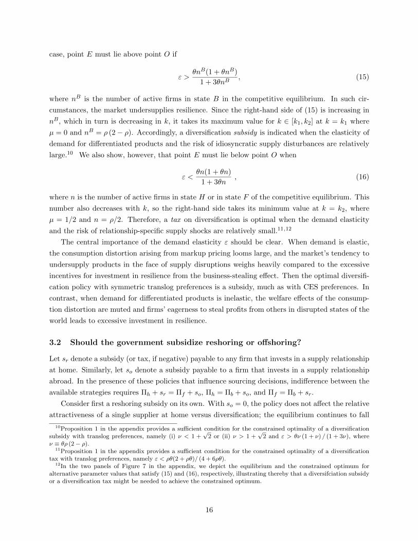
k0

µf = 0µh = 0µb = 1

k1 k2

0 < µf = µhµb > 0

k3

µf = µh = 1/2µb = 0

k4

0 < µf = µh < 1/2µb = 0

No investment

Figure 1:Supply Chain Outcomes: Symmetric Case

Firms that diversify earn profits in both states H and F , whereas those that maintain a single

relationship earn profits only in one of these states. Those that diversify also stand a better chance

of surviving in state B, when relationship-specific shocks might disrupt their individual supply

chains. Evidently, diversified firms enjoy higher expected operating profits. But they also pay an

added fixed cost. The choice of whether to diversify hinges on the size of the fixed cost; for example,

Πb > Πh if and only if k < δFπFρ+ δBπBρ (1− ρ).

Figure 1 depicts the outcome as a function of k. For low enough k, i.e., k < k1, firms view

the insurance against supply disruptions as well worth the extra cost and all firms diversify. For

the next range of fixed costs between k1 and k2, all available strategies are used in equilibrium

by positive numbers of firms, with µh = µf = µ rising in k, and µb = 1 − 2µ declining in k. All

firms in the industry invest in at least one supply relationships. At fixed costs above k2, it is no

longer profitable for any firm to invest in resilience, because the potential profits in the event of a

disruption do not justify the extra fixed cost of a second relationship. All firms continue to pursue

either strategy h or strategy f (with equal number of each) for k ∈ (k2, k3), whereas the total

number of firms that form a relationship declines with k when k ∈ (k3, k4).5 Finally, at k4 and

above, fixed costs are so high as to render entry unprofitable for all modes of organization.6

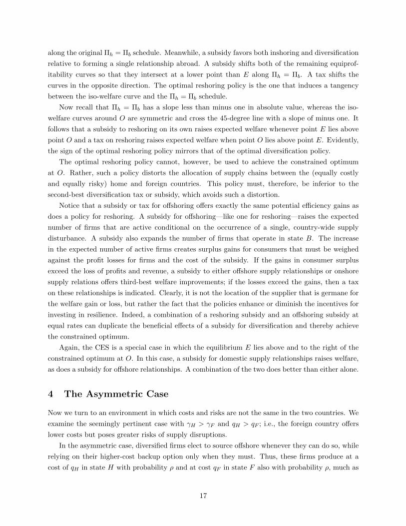
In Figure 2, we illustrate an equilibrium at E for a typical (symmetric) case with k ∈ (k1, k2).

The figure shows µh and µf on the vertical and horizontal axes, respectively. Since k is in the

range where all firms invest in at least one supply relationship, Figure 2 depicts the plane in

(µf , µh, µb) space along which µb = 1 − µf − µh. We have already argued that, for any value of

µb, equiprofitability of the onshore and offshore options requires µh = µf . Therefore, the 45-degree

line shows combinations of µh and µf such that single relationships at home and abroad are equally

profitable.

The downward sloping curve labelled Πh = Πb shows combinations of µh and µf (with µb =

1 − µf − µh) for which investing in a single relationship at home yields the same expected profits

as a strategy of diversification. Note that, with δH = δF , (11) and (13) yield the equation for this

curve,

γ (1− γ)πFρ+ γ2πBρ (1− ρ) = k. (14)

The downward slope of the curve can be understood as follows. Starting from a point on the

5For k ∈ (k2, k3), Πh = Πf > 0 > Πb, whereas for k ∈ (k3, k4), Πh = Πf = 0 > Πb.6If profits go to infinity as µ→ (0, 0, 0), then k3 →∞ as well. Entry always is profitable for finite k, for example,

if U (·) takes the CES form.

12

µf

µh

1

10

Πh = Πf

45o

Πh = Πb

Πf = Πb

E

O

Figure 2:Equilibrium and Constrained Optimum for Symmetric Case

curve, say E, suppose we move vertically upward. This shift corresponds to a rise in µh and a

decline in µb of similar magnitudes, with µf held constant. The change in composition of strategies

does not affect the total number of firms active in state H, but it decreases the numbers of firms

active in states F and B. Thus, πF and πB rise, leaving a (positive) gap between Πb and Πh for

points vertically above E.7 Now consider a fall in µf accompanied by an offsetting rise in µb at a

given µh, i.e., a horizontal movement to the left. This change in the composition of firms intensifies

competition in state H, which contributes to lower expected profits for both h firms and b firms.

Since both types earn operating profits of πH with the same probability ρ in state H, the fall

in πH does not figure in the comparison between the two. Meanwhile, in state F , the offsetting

changes in µf and µb leave the intensity of competition untouched and with it the operating profits

πF for any firm that is active in this state. Finally, in state B, the number of active firms rises,

because a given firm is more likely to produce in this state if it is diversified than if it has only a

single potential supplier. The intensification of competition in state B reduces πB, which depresses

expected profits more for diversified firms than for those that invest only in a domestic supplier,

because the former firms are more likely to survive in this state. Thus, a decrease in µf offset by

an increase in µb reduces Πb relative to Πh. It follows that a decrease in µf is needed to offset the

effects of an increase in µh if strategies h and b are to be equally profitable. We note further that

7The fall in competition in state F serves to increase expected profits of diversified firms, but does not affect theexpected profits of firms that can only source at home. The fall in competition in state B raises the profitability ofan active h firm and an active b firm by similar amounts, but the diversified firms have a better chance of avoidingsupply disruptions, so they reap a bigger boost to expected profits in this state as well.

13

the Πh = Πb curve must have a slope less than one in absolute value.8

The curve labelled Πf = Πb shows combinations of µh and µf for which investing in a single

relationship abroad yields the same expected profits as a strategy of diversification. It too slopes

downward, for analogous reasons, and the curve must have a slope greater than one in absolute

value. Finally, the three curves intersect at E, where all three strategies are equally profitable, as

befits an equilibrium in which positive numbers of firms select each option.

The figure also illustrates a constrained optimum at O. The constrained optimum does not

achieve maximal expected welfare for the home country, because it maximizes W over the choice

of µ in the presence of monopoly pricing of differentiated products. In the appendix, we show

that the first-order conditions for a constrained maximum are satisfied with an appropriate choice

of µh = µf for any HSA preferences. We also show that the welfare function W (µ) is globally

concave when U (X) takes a CES form and that the constrained optimum must have µh = µf when

preferences take the symmetric translog form. Evaluating the second-order conditions for more

general HSA preferences is challenging, but it seems compelling that the planner would want equal

numbers of firms with single relationships at home and abroad. The figure depicts some iso-welfare

loci for successively lower levels of expected welfare as we move away from O. Notice that they are

symmetric about the 45-degree line, thanks to the symmetry across countries.

3.1 Should the government subsidize diversification?

In the symmetric case, a diversification policy alone can be used to achieve the constrained optimum.

Suppose the government provides a subsidy of sd to firms that add a second supplier (with sd < 0

representing a tax). Such a subsidy has no effect on the profitability of engaging a single supplier,

be it at home or abroad. Therefore, the curve that represents equiprofitability of the alternative

locations for single suppliers continues to be the 45-degree line from the origin. With a subsidy

(or tax) in place, indifference between investing in a single relationship and investing in resilience

requires Πj = Πb + sd for j = h, f . Clearly, a subsidy of this sort shifts the curve representing

indifference between h and b and that representing indifference between f and b downward, while

a tax shifts these curves in the opposite direction. If point E lies above point O on the 45-degree

line (as depicted in Figure 2), then a diversification subsidy can be used to achieve the constrained

optimum. If point O lies above point E, the government needs to discourage diversification in order

to achieve the constrained optimum. In general, either outcome is possible.

In the special case of CES preferences, however, point E always lies above pointO, so the optimal

policy that achieves the second best is a subsidy for diversification. By promoting resilience, the

government augments the availability of products in all three states. In states H and F , the number

of active firms increases by (ρ/2) ∆µb > 0, because µh + µf + µb = 1 and µh = µf = µ imply

∆µh = ∆µf = −∆µb/2. In state B, the number of active firms increases by ρ (1− ρ) ∆µb > 0,

8The effect on expected profits of a diversified firm relative to a home-only firm conditional on state B are equaland opposite for a given increase in µh and comparable decrease in µf . But the increase in µh (and accompanyingdecrease in µb) gives an added boost to the relative profitability of diversification, because it raises the expectedprofits for a b firm if state F arises. See the appendix for more details.

14

because nB = (µh + µf + µb) ρ + ρ (1− ρ)µb and µh + µf + µb = 1. The increase in available

products in each state boosts aggregate welfare, because the market undersupplies diversity in the

CES case with an outside good.9

The gains from promoting resilience in the CES case can best be understood by considering a

combination policy of a tax or subsidy on diversification and a hypothetical subsidy to consumption

of differentiated products. The latter policy (if feasible) could serve to counteract the distortion

caused by monopoly pricing, so that consumers face the marginal cost, q. We show in the appendix

that, once the consumption distortion has been eliminated in this way, there is no further need for

a policy to promote diversification; indeed, the first-best outcome is achieved by a consumption

subsidy alone, with zero tax or subsidy on supply-chain formation. Only when a consumption

subsidy is infeasible does it become beneficial to promote resilience. With constant markup pricing

in one sector and competitive pricing in the other, the consumer surplus of an additional product

exceeds the cost of bringing it to market. A diversification subsidy generates second-best gains by

creating greater product availability in every state of nature.

What if the elasticity of substitution is not constant but instead rises with price, per Marshall’s

Second Law of Demand? In the appendix, we prove that the first best can be achieved with a

subsidy to consumption and a tax on diversification. This finding echoes Matsuyama and Ushchev

(2020), who show that, in a setting of monopolistic competition with a single sector, the market

oversupplies diversity with HSA preferences when the elasticity of substitution increases with price.

The explanation they give is that, with σ′ (z) > 0, the business-stealing effect dominates the

consumer-surplus effect, i.e., the fact that firms do not take account of the effect of their entry on

the profits of others overrides the fact that they do not take account of the surplus they generate

for consumers. The excessive incentive for entry that they describe translates into an excessive

incentive for firms to diversify their supply chains in order to boost the likelihood that they can

operate in the face of supply disruptions.

In the setting studied by Matsuyama and Ushchev (2020), markup pricing by homogeneous

firms does not create any consumption distortion, because relative prices are not affected by firms’

uniform markup pricing. Therefore, the powerful incentives for business stealing under MSLD

generate socially excessive entry in the monopolistically competitive equilibrium. Had they allowed

for a second sector with competitive pricing, their conclusion would have been more nuanced, much

as ours is here. Excessive incentives for business stealing on its own suggests too much investment

in resilience, but distorted relative prices across industries imply the opposite. Accordingly, the

government might need either to promote or to discourage diversification in order to achieve the

constrained optimum.

Investigation of the case of symmetric translog preferences affords some additional insight.

Recall that, with these preferences, s (z) = −θ log z. In the appendix we show that, in the translog

9See the proof in the appendix. For an analogous result in a world without supply shocks, see, for example,Campolmi, Fadinger and Forlati (2021).

15

case, point E must lie above point O if

ε >θnB(1 + θnB)

1 + 3θnB, (15)

where nB is the number of active firms in state B in the competitive equilibrium. In such cir-

cumstances, the market undersupplies resilience. Since the right-hand side of (15) is increasing in

nB, which in turn is decreasing in k, it takes its maximum value for k ∈ [k1, k2] at k = k1 where

µ = 0 and nB = ρ (2− ρ). Accordingly, a diversification subsidy is indicated when the elasticity of

demand for differentiated products and the risk of idiosyncratic supply disturbances are relatively

large.10 We also show, however, that point E must lie below point O when

ε <θn(1 + θn)

1 + 3θn, (16)

where n is the number of active firms in state H or in state F of the competitive equilibrium. This

number also decreases with k, so the right-hand side takes its minimum value at k = k2, where

µ = 1/2 and n = ρ/2. Therefore, a tax on diversification is optimal when the demand elasticity

and the risk of relationship-specific supply shocks are relatively small.11,12

The central importance of the demand elasticity ε should be clear. When demand is elastic,

the consumption distortion arising from markup pricing looms large, and the market’s tendency to

undersupply products in the face of supply disruptions weighs heavily compared to the excessive

incentives for investment in resilience from the business-stealing effect. Then the optimal diversifi-

cation policy with symmetric translog preferences is a subsidy, much as with CES preferences. In

contrast, when demand for differentiated products is inelastic, the welfare effects of the consump-

tion distortion are muted and firms’ eagerness to steal profits from others in disrupted states of the

world leads to excessive investment in resilience.

3.2 Should the government subsidize reshoring or offshoring?

Let sr denote a subsidy (or tax, if negative) payable to any firm that invests in a supply relationship

at home. Similarly, let so denote a subsidy payable to a firm that invests in a supply relationship

abroad. In the presence of these policies that influence sourcing decisions, indifference between the

available strategies requires Πh + sr = Πf + so, Πh = Πb + so, and Πf = Πb + sr.

Consider first a reshoring subsidy on its own. With so = 0, the policy does not affect the relative

attractiveness of a single supplier at home versus diversification; the equilibrium continues to fall

10Proposition 1 in the appendix provides a sufficient condition for the constrained optimality of a diversificationsubsidy with translog preferences, namely (i) ν < 1 +

√2 or (ii) ν > 1 +

√2 and ε > θν (1 + ν) / (1 + 3ν), where

ν ≡ θρ (2− ρ).11Proposition 1 in the appendix provides a sufficient condition for the constrained optimality of a diversification

tax with translog preferences, namely ε < ρθ(2 + ρθ)/ (4 + 6ρθ).12In the two panels of Figure 7 in the appendix, we depict the equilibrium and the constrained optimum for

alternative parameter values that satisfy (15) and (16), respectively, illustrating thereby that a diversifciation subsidyor a diversification tax might be needed to achieve the constrained optimum.

16

along the original Πh = Πb schedule. Meanwhile, a subsidy favors both inshoring and diversification

relative to forming a single relationship abroad. A subsidy shifts both of the remaining equiprof-

itability curves so that they intersect at a lower point than E along Πh = Πb. A tax shifts the

curves in the opposite direction. The optimal reshoring policy is the one that induces a tangency

between the iso-welfare curve and the Πh = Πb schedule.

Now recall that Πh = Πb has a slope less than minus one in absolute value, whereas the iso-

welfare curves around O are symmetric and cross the 45-degree line with a slope of minus one. It

follows that a subsidy to reshoring on its own raises expected welfare whenever point E lies above

point O and a tax on reshoring raises expected welfare when point O lies above point E. Evidently,

the sign of the optimal reshoring policy mirrors that of the optimal diversification policy.

The optimal reshoring policy cannot, however, be used to achieve the constrained optimum

at O. Rather, such a policy distorts the allocation of supply chains between the (equally costly

and equally risky) home and foreign countries. This policy must, therefore, be inferior to the

second-best diversification tax or subsidy, which avoids such a distortion.

Notice that a subsidy or tax for offshoring offers exactly the same potential efficiency gains as

does a policy for reshoring. A subsidy for offshoring—like one for reshoring—raises the expected

number of firms that are active conditional on the occurrence of a single, country-wide supply

disturbance. A subsidy also expands the number of firms that operate in state B. The increase

in the expected number of active firms creates surplus gains for consumers that must be weighed

against the profit losses for firms and the cost of the subsidy. If the gains in consumer surplus

exceed the loss of profits and revenue, a subsidy to either offshore supply relationships or onshore

supply relations offers third-best welfare improvements; if the losses exceed the gains, then a tax

on these relationships is indicated. Clearly, it is not the location of the supplier that is germane for

the welfare gain or loss, but rather the fact that the policies enhance or diminish the incentives for

investing in resilience. Indeed, a combination of a reshoring subsidy and an offshoring subsidy at

equal rates can duplicate the beneficial effects of a subsidy for diversification and thereby achieve

the constrained optimum.

Again, the CES is a special case in which the equilibrium E lies above and to the right of the

constrained optimum at O. In this case, a subsidy for domestic supply relationships raises welfare,

as does a subsidy for offshore relationships. A combination of the two does better than either alone.

4 The Asymmetric Case

Now we turn to an environment in which costs and risks are not the same in the two countries. We

examine the seemingly pertinent case with γH > γF and qH > qF ; i.e., the foreign country offers

lower costs but poses greater risks of supply disruptions.

In the asymmetric case, diversified firms elect to source offshore whenever they can do so, while

relying on their higher-cost backup option only when they must. Thus, these firms produce at a

cost of qH in state H with probability ρ and at cost qF in state F also with probability ρ, much as

17

do firms with sole suppliers in country H or in country F , respectively. In state B, the diversified

firms produce at cost qF with probability ρ and at cost qH with probability ρ (1− ρ).

We denote by zB,i the relative price charged by a firm in state B that sources from country i,

i = H,F . Market shares must sum to one in every state, which gives (9) as before for J ∈ H,F.In state B, we have

1 = nB,H (µ) s(zB,H

)+ nB,F (µ) s

(zB,F

), (17)

where nB,i is the number of active firms in state B that source from country i and so nB,F =

(1− µh) ρ and nB,H = µhρ + µbρ (1− ρ) = (1− µf ) ρ (1− ρ) + µhρ2. The pricing equation (6)

implies

zB,H

zB,F=

σ(zB,H)σ(zB,H)−1

σ(zB,F )σ(zB,F )−1

qHqF

. (18)

Now we can use (9) for J = H,F together with (17) and (18) to solve for the four relative-price

terms as functions of µ.

Operating profits for firms that do not suffer supply disruptions are given by

π(zJ)

=s(zJ)

σ (zJ)P(zJ)1−ε

, for J = H,F,

and

πB,i = πB,i(zB,i;nB, zB

)=s(zB,i

)σ (zB,i)

P(nB, zB

)1−ε, i = H,F ,

where nB =(nB,H , nB,F

)and zB =

(zB,H , zB,F

). Finally, we calculate the expected profits

associated with each strategy,

Πh = δHπ(zH)ρ+ δBπB,H

(zB,H

)ρ− k ,

Πf = δFπ(zF)ρ+ δBπB,F

(zB,F

)ρ− k ,

and

Πb = δHπ(zH)ρ+ δFπ

(zF)ρ+ δBπB,F

(zB,F

)ρ+ δBπB,H

(zB,H

)ρ (1− ρ)− 2k ,

with δH = γH (1− γF ), δF = γF (1− γH), and δB = γHγF . These expected profit levels are all

functions of µ.

Figure 3 shows the fraction of firms that choose each organizational form for different values of

k. For k < k1, all firms find it worthwhile to invest in resilience, so µb = 1 and µh = µf = 0. Next

comes a range of fixed cost for which some firms are diversified, and others form relationships in

a single country, with all sole-source suppliers located either in country H or in country F . The

figure depicts a case with qH ≈ qF and γH > γF . In such circumstances, there exists a k2 such that

for k ∈ (k1, k2), µh = 1 − µb > 0 and µf = 0. Alternatively if qF < qH and γH ≈ γF , then there

18

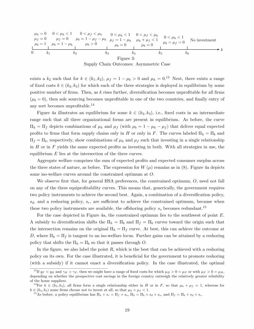
k0

µh = 0µf = 0µb = 1

k1 k2 k3 k4 k5 k6

0 < µh < 1µf = 0

µb = 1− µh

0 < µf < µhµb = 1− µf − µh

µb > 0

0 < µh < 1µf = 1− µhµb = 0

0 < µf < µhµh + µf < 1µb = 0

0 < µh < 1µb = µf = 0

No investment

Figure 3:Supply Chain Outcomes: Asymmetric Case

exists a k2 such that for k ∈ (k1, k2), µf = 1 − µb > 0 and µh = 0.13 Next, there exists a range

of fixed costs k ∈ (k2, k3) for which each of the three strategies is deployed in equilibrium by some

positive number of firms. Then, as k rises further, diversification becomes unprofitable for all firms

(µb = 0), then sole sourcing becomes unprofitable in one of the two countries, and finally entry of

any sort becomes unprofitable.14

Figure 4a illustrates an equilibrium for some k ∈ (k2, k3), i.e., fixed costs in an intermediate

range such that all three organizational forms are present in equilibrium. As before, the curve

Πh = Πf depicts combinations of µh and µf (with µb = 1 − µh − µf ) that deliver equal expected

profits to firms that form supply chains only in H or only in F . The curves labeled Πh = Πb and

Πf = Πb, respectively, show combinations of µh and µf such that investing in a single relationship

in H or in F yields the same expected profits as investing in both. With all strategies in use, the

equilibrium E lies at the intersection of the three curves.

Aggregate welfare comprises the sum of expected profits and expected consumer surplus across

the three states of nature, as before. The expression for W (µ) remains as in (8). Figure 4a depicts

some iso-welfare curves around the constrained optimum at O.

We observe first that, for general HSA preferences, the constrained optimum, O, need not fall

on any of the three equiprofitability curves. This means that, generically, the government requires

two policy instruments to achieve the second best. Again, a combination of a diversification policy,

sd, and a reshoring policy, sr, are sufficient to achieve the constrained optimum, because when

these two policy instruments are available, the offshoring policy so becomes redundant.15

For the case depicted in Figure 4a, the constrained optimum lies to the southwest of point E.

A subsidy to diversification shifts the Πh = Πb and Πf = Πb curves toward the origin such that

the intersection remains on the original Πh = Πf curve. At best, this can achieve the outcome at

D, where Πh = Πf is tangent to an iso-welfare locus. Further gains can be attained by a reshoring

policy that shifts the Πh = Πb so that it passes through O.

In the figure, we also label the point R, which is the best that can be achieved with a reshoring

policy on its own. For the case illustrated, it is beneficial for the government to promote reshoring

(with a subsidy) if it cannot enact a diversification policy. In the case illustrated, the optimal

13If qF < qH and γH > γF , then we might have a range of fixed costs for which µH > 0 = µF or with µF > 0 = µH ,depending on whether the prospective cost savings in the foreign country outweigh the relatively greater reliabilityof the home suppliers.

14For k ∈ (k3, k4), all firms form a single relationship either in H or in F , so that µh + µf = 1, whereas fork ∈ (k4, k5) some firms choose not to invest at all, so that µh + µf < 1.

15As before, a policy equilibrium has Πh + sr = Πf + so, Πh = Πb + sd + so, and Πf = Πb + sd + sr.

19

µf

µh

0

1

1

O

ER

DΠh = Πb

Πh = Πf

Πf = Πb

(a) General HSA Preferences

µf

µh

0

1

1

O

ER

FΠh = Πb

Πh = Πf

Πf = Πb

(b) CES Preferences

Figure 4:Equilibrium and Constrained Optimum for Asymmetric Case

reshoring policy does not yield as high a level of expected welfare as the optimal diversification

policy.

Let us turn to the special case of CES preferences, as depicted in Figure 4b. In this case,

consumer surplus in any state of nature J is proportional to the price index, P J , raised to the

power of 1− ε. Meanwhile, profits in state J of any active firm are proportional to the same term,(P J)1−ε

. We show in the appendix that—due to this exceptional feature of the CES, which reflects

the dual role of the price index as both single aggregator and welfare metric—the constrained

optimum satisfies Πh = Πf . In other words, the point O must lie on the Πh = Πf curve, much like

the equilibrium point E.

The fact that the constrained optimum falls on the Πh = Πf curve means that the second

best can be achieved with a single policy instrument, namely a tax or subsidy for diversification.

A subsidy shifts the equilibrium downward from E, whereas a tax shifts the equilibrium upward.

However, as we also show in the appendix, point O always lies below point E on the Πh = Πf

curve, so, with CES preferences, it is always desirable for the government to promote resiliency

with a subsidy for all values of the cost and risk parameters. The explanation is the same as in

the symmetric case; in the CES case, the market underprovides resiliency, because the consumer

surplus plus profit gains from greater product availability in a given state exceeds the fixed cost of

another link in the supply chain. This conclusion reflects the fixed and positive wedge that exists

with constant-markup pricing between consumer prices and marginal costs.

In Figure 4b we also see that either a subsidy for supply relationships at home or a subsidy

for supply relationships abroad can be used to raise expected welfare relative to the equilibrium at

E, although neither of these policies can achieve the second-best level of welfare that is attainable

20

with the optimal diversification subsidy.16 The optimal reshoring subsidy shifts the equilibrium to

point R, whereas the optimal offshoring subsidy shifts the equilibrium to point F . These outcomes

cannot be uniquely ranked without further information about relative costs and risks.

Moving beyond CES, some results from the symmetric case generalize. For example, if con-

sumers have symmetric translog preferences and the costs in the two countries do not differ by too

much, then the optimal diversification policy promotes resilience when ε is large but discourages

resilience for ε is small. But, with asymmetric costs and risks, HSA preferences admit a richer set

of possibilities. For example, any of the three policy instruments (diversification tax or subsidy,

reshoring tax or subsidy or offshoring tax or subsidy) might offer the greatest welfare improvement

if the government can only implement one such policy. General results are difficult to come by, so

we rely instead on numerical analysis to explore some of the possibilities. We highlight in particular

how policy recommendations might reflect differences in the likelihood of supply chain disruptions

at home and abroad.

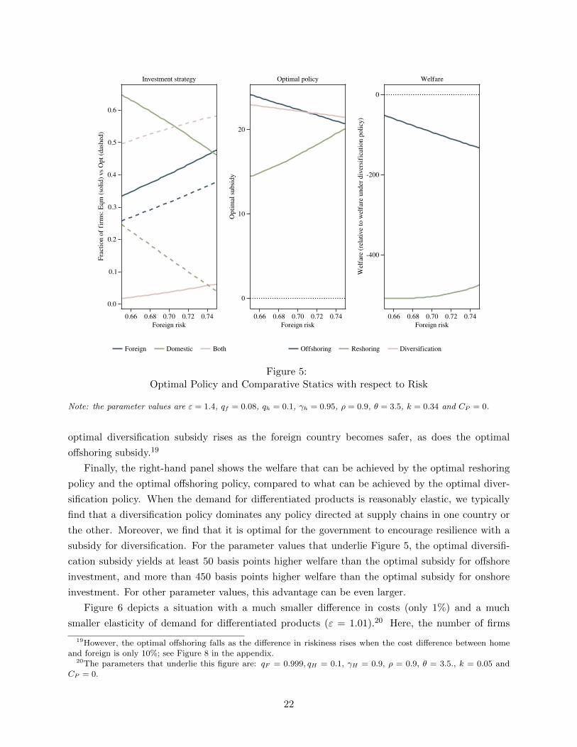
Figure 5 depicts a reasonably typical case with symmetric translog preferences.17 We take the

translog parameter θ = 3.5, the relationship-specific probability of supply disruption 1 − ρ = 0.1,

the elasticity of demand for differentiated products ε = 1.4, and the respective unit costs of the

input qH = 0.1 and qF = 0.08, so that the cost advantage of the foreign country is 20%. The other

parameters were chosen to ensure that all three strategies are used by some firms in equilibrium.18

The left-hand panel in the figure shows the fractions of firms that adopt each strategy (solid

curves) and the constrained-optimal fractions (dashed curves) for each mode of operation for various

degrees of risk asymmetry. The figure shows that too many firms establish a single relationship in

the safer home market compared to the constrained optimum. This finding is very common in our

numerical analysis. The excessive home sourcing often (but not always) comes at the expense of

too little diversification, with single supplier relationships abroad also above the efficient level.

Not surprisingly, as the risk of foreign supply disruptions falls, both the equilibrium and optimal

number of firms that invest in a single relationship at home declines. Meanwhile, the number of

firms that invest in some manner in a supply relationship abroad grows. These new relationships

might take the form of more single relationships abroad (µf increases) or more diversified firms (µb

increases), or both. The figure depicts a case in which both µf and µb rise with γF , but it is not

difficult to find reasonable parameter values for which one or the other falls.

The middle panel shows the size of the optimal subsidies for diversification, reshoring, and

offshoring, as functions of relative risk. With ε = 1.4, the market accepts too much risk of disruption

compared to the constrained optimum. Therefore, all three optimal subsidies are positive. The

16The iso-welfare curves have a slope of minus one where they cross the Πh = Πf curves, just as in the symmetriccase. And the Πh = Πb and Πf = Πb have slopes at less than and greater than one in absolute value, respectively,where they cross Πh = Πf , as drawn; see the appendix for the proof. This implies that a subsidy to reshoring oroffshoring raises welfare, because they move the equilbrium to the left along the original Πh = Πb curve or to theright along the original Πf = Πb curve, respetively, in each case shifting onto an iso-welfare contour representing ahigher level of welfare.

17A range of other numerical examples are provided in Figures 8-11 in the appendix.18More specifically, the figure assumes γH = 0.95, k = 0.34 and CP = 0.

21

Foreign risk0.66 0.68 0.70 0.72 0.74

Fra

ctio

n of

fir

ms:

Eqm

(so

lid)

vs O

pt (

dash

ed)

0.0

0.1

0.2

0.3

0.4

0.5

0.6

Investment strategy

Foreign risk0.66 0.68 0.70 0.72 0.74

Opt

imal

sub

sidy

0

10

20

Optimal policy

Foreign risk0.66 0.68 0.70 0.72 0.74

Wel

fare

(re

lati

ve to

wel

fare

und

er d

iver

sifi

cati

on p

olic

y)

-400

-200

0

Welfare

Foreign Domestic Both Offshoring Reshoring Diversification

Figure 5:Optimal Policy and Comparative Statics with respect to Risk

Note: the parameter values are ε = 1.4, qf = 0.08, qh = 0.1, γh = 0.95, ρ = 0.9, θ = 3.5, k = 0.34 and CP = 0.

optimal diversification subsidy rises as the foreign country becomes safer, as does the optimal

offshoring subsidy.19

Finally, the right-hand panel shows the welfare that can be achieved by the optimal reshoring

policy and the optimal offshoring policy, compared to what can be achieved by the optimal diver-

sification policy. When the demand for differentiated products is reasonably elastic, we typically

find that a diversification policy dominates any policy directed at supply chains in one country or

the other. Moreover, we find that it is optimal for the government to encourage resilience with a

subsidy for diversification. For the parameter values that underlie Figure 5, the optimal diversifi-

cation subsidy yields at least 50 basis points higher welfare than the optimal subsidy for offshore

investment, and more than 450 basis points higher welfare than the optimal subsidy for onshore

investment. For other parameter values, this advantage can be even larger.

Figure 6 depicts a situation with a much smaller difference in costs (only 1%) and a much

smaller elasticity of demand for differentiated products (ε = 1.01).20 Here, the number of firms

19However, the optimal offshoring falls as the difference in riskiness rises when the cost difference between homeand foreign is only 10%; see Figure 8 in the appendix.

20The parameters that underlie this figure are: qF = 0.999, qH = 0.1, γH = 0.9, ρ = 0.9, θ = 3.5., k = 0.05 andCP = 0.

22

Foreign risk0.86 0.87 0.88 0.89

Fra

ctio

n of

fir

ms:

Eqm

(so

lid)

vs O

pt (

dash

ed)

0.0

0.2

0.4

0.6

0.8

Investment strategy

Foreign risk0.86 0.87 0.88 0.89

Opt

imal

sub

sidy

-8

-6

-4

-2

0

Optimal policy

Foreign risk0.86 0.87 0.88 0.89

Wel

fare

(re

lati

ve to

wel

fare

und

er d

iver

sifi

cati

on p

olic

y)

-0.10

-0.05

0.00

Welfare

Foreign Domestic Both Offshoring Reshoring Diversification

Figure 6:Optimal Policy and Comparative Statics with respect to Risk: Small Cost Difference and ε = 1.01

Note: the parameter values are ε = 1.01, qf = 0.099, qh = 0.1, γh = 0.9, ρ = 0.9, θ = 3.5, k = 0.05 and CP = 0.

that diversify in equilibrium exceeds the socially optimal level, at the expense of firms that form

single relationships both at home and abroad. Overall, the equilibrium provides excessive resilience,

so it is optimal to tax diversification (see middle panel) or, if that is not possible, to discourage

supply chain formation at home or abroad. The right-hand panel shows that a diversification tax

dominates a tax on offshoring, whereas the relative ranking of the optimal diversification tax and

the optimal reshoring tax depends on the size of the risk gap. However, for all values of γF , the

difference in welfare is quite narrow, amounting to only a small fraction of one basis point. The

tiny welfare effects are quite typical when unit costs are similar and ε differs little from one.

5 Conclusions

Supply chain disruptions are increasingly salient and often quite costly. Many commentators have

been quick to conclude that governments ought to be doing something to promote greater market

resilience. But the welfare-theoretic calculus around government intervention is rather subtle. Pri-

vate actors have a clear self-interest in taking measures to avoid disruptions to their production

processes. Only when the private incentives for resilience fall short of the social benefits will gov-

23

ernment encouragement be warranted. Pointing in that direction is the observation that consumers

capture part of the surplus created by the ongoing availability of firms’ products. But firms also

have an incentive to be in a position to reap extra profits when their rivals are suffering. The

temptation for “business stealing” suggests that excess resilience is also a possible market outcome.

Surprisingly little research has addressed the desirability of government policy to promote re-

silience or to encourage sourcing from safer locations. In this paper, we have taken a first step.

We have proposed a simple framework in which the supply of any product requires the availability

of a critical input. Exogenous shocks can disrupt the firms’ relationships with their suppliers. We

allow for idiosyncratic shocks that affect a single relationship and broader shocks that impinge

on all sourcing from a particular country or region. Firms face the choice of where to develop

a relationship and whether to protect their operation with backup sources of supply. We study

the simplest case of two potential supply sources, one at home and one abroad and focus on a

situation where domestic sourcing is (weakly) costlier than sourcing abroad, but also (weakly) less

risky. This setting presents firms with three options: invest in a single supply relationship at home

(onshoring), invest in a single relationship abroad (offshoring), or invest in supply relationships in

both locations (diversification).

Since consumer gains from product availability reflect their preferences, the form of demand

plays a critical role in the policy calculus. The CES demand system is popular and tractable for

analysis such as ours. But it also introduces restrictions that may color the findings. We allow for a

CES utility function, but also for a broader class of preferences that Matsuyama and Ushchev (2020)

have developed and termed Homothetic with a Single Aggregator. The more general preferences

admit non-constant markups and, in particular, application of Marshall’s Second Law of Demand.

Our analysis yields several broad lessons. First, the government generally needs at least two

policy instruments to achieve efficient sourcing, once allowance is made for the existence of markup

pricing. One instrument regulates the margin between sourcing from one location or two. The

other guides the choice between sourcing at home and abroad. For example, the government might

subsidize or tax supply-chain diversification, while subsidizing or taxing onshoring. Or it might

subsidize or tax diversification, while subsidizing or taxing offshoring. However, when preferences

take the CES form, one instrument suffices to achieve the constrained optimum, namely a policy

to promote diversification. In the CES case, even when the home and foreign sources bear different

costs and risks, the private and social incentives to source at home and abroad coincide once the

correct incentives for diversification have been created.

Second, when the government is limited to use only one policy instrument, either a policy

that encourages or discourages diversification or one that alters the incentives for relationships in

one country or the other might achieve a superior outcome. And the second best policy might

be a subsidy or a tax. In the CES case, a diversification policy dominates a reshoring policy or

an offshoring policy, and a subsidy (as opposed to a tax) for diversification is indicated. More

generally, a high elasticity of demand for differentiated products tends to favor diversification

subsidies whereas a low elasticity of demand for this group of products opens the possibility that

24

a tax will be optimal. This finding reflects the fact that markup pricing creates an undersupply

of product diversity in the market equilibrium that is especially pronounced when demand for

differentiated products is highly elastic. In contrast, when demand is not so elastic, the private

gains from potential business stealing may lead firms to overinvest in resilience.

Our paper opens the door to further research. For example, we have considered only the

simplest possible production process whereby each firm produces a final product from a single

critical input. Our framework could be extended to allow for more complex supply chains, including

multiple purchased inputs from various sources that might also be combined with primary factors

of production. We could also examine a sequential production process whereby some inputs enter

into production upstream from others. Then we could ask whether the need for resilience or for safe

sources of supply is more important for upstream inputs or downstream inputs and how private

and social incentives differ at various stages. Further, we could introduce possibilities for storage

in a multi-period model, so that firms might invest in resilience by stockpiling inputs and the

government might promote availability by holding reserves of consumer goods. Issues of supply

chain disruption are bound to be with us for a while and many important policy questions remain

to be addressed.

25

References

[1] Arad, Ruth W. and Arye L. Hillman, 1979. “Embargo Threat, Learning and Departure from

Comparative Advantage,” Journal of International Economics 9, 265-275.

[2] Bergstrom, Clas, Loury, Glenn C. and Mats Persson, 1985. “Embargo Threats and the Man-

agement of Emergency Reserves, Journal of Political Economy 93(1), 26-42.

[3] Bhagwati, Jagdish N. and T.N. Srinivasan, 1976. “Optimal Trade Policy and Compensation

under Endogenous Uncertainty: The Phenomenon of Market Disruption,” Journal of Interna-

tional Economics 6, 317-336.

[4] Campolmi, Alessia, Fadinger, Harald, and Chiata Forlati, 2021. “Trade and Do-

mestic Policies in Models with Monopolistic Competition,” http://fadinger.vwl.uni-

mannheim.de/Research files/CFF 20210722.pdf.

[5] Carvalho, Vasco M., Nirei, Makoto, Saito, Yukiko U. and Alifrez Tahbaz-Salehi, 2021. “Supply

Chain Disruptions: Evidence from the Great East Japan Earthquake,” Quarterly Journal of

Economics 136(2): 1255-1321.

[6] Cheng, Leonard K., 1989. “Intermittent Trade Disruptions and Optimal Production,” Inter-

national Economic Review 30(4): 753-74.

[7] Dhingra, Swati and John Morrow, 2019. “Monopolistic Competition and Optimum Product

Diversity under Firm Heterogeneity,” Journal of Political Economy 127(1), 196-232.

[8] Diewert, W.E., 1974. “Applications of Duality Theory,” in M. Intriligator and D. Kendrick

(eds.), Frontiers of Quantitative Economics, vol. II, Amsterdam: North Holland.

[9] Dixit, Avinash K. and Joseph E. Stiglitz, 1977. “Monopolistic Competition and Optimum

Product Diversity,” American Economic Review 67(3): 297-308.

[10] Feenstra, Robert C., 2003. “A Homothetic Utility Function for Monopolistic Competition

Models, without Constant Price Elasticity,” Economic Letters 78(1): 79-86.

[11] Iakovou, Eleftherios and Chelsea C. White III, 2020. “How to Build More Secure, Resilient,

Next-Gen U.S. Supply Chains,” TechStream, Brookings Institution.

[12] Matsuyama, Kiminori and Philip Ushchev, 2020. “When Does Procompetitive Entry Imply

Excessive Entry,” CEPR Discussion Paper No. 14991.

[13] Mayer, Wolfgang, 1977. “The National Defense Tariff Argument Reconsidered,” Journal of

International Economics 7, 363-77.

[14] McKinsey Global Institute, 2020. Risk, Resilience and Rebalancing in Global Value Chains.

26

[15] Melitz, Marc J., 2018. “Competitive Effects of Trade: Theory and Measurement,” Review of

World Economics 154, 1-13.

[16] Mrazova, Monika and J. Peter Neary, 2017. “Not So Demanding: Demand Structure and Firm

Behavior,” American Economic Review 107(12): 3835-74.

[17] Shih, Willy C., 2020a. “Global Supply Chains in a Post-Pandemic World,” Harvard Business

Review 98(5): 82-9.

[18] Shih, Willy C., 2020b. “Is it Time to Rethink Globalized Supply Chains,” MIT Sloan Man-

agement Review 61(4): 16-18.

[19] Zhelobodko, Evgeny. Kokovin, Sergey, Parenti, Mathieu and Jacques-Francois Thisse, 2012.

“Monopolistic Competition: Beyond the Elasticity of Substitution,” Econometrica 80(6):

2765-2784.

27

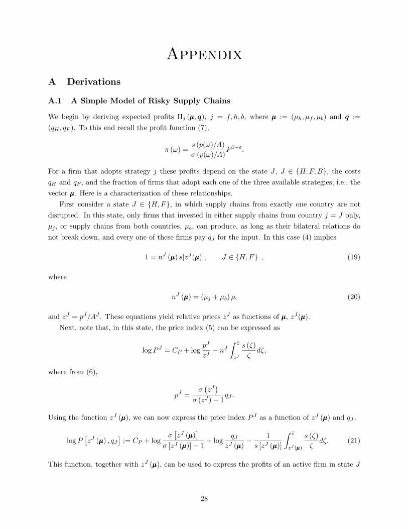
Appendix

A Derivations

A.1 A Simple Model of Risky Supply Chains

We begin by deriving expected profits Πj (µµµ, q), j = f, h, b, where µµµ := (µh, µf , µb) and q :=

(qH , qF ). To this end recall the profit function (7),

π (ω) =s (p(ω)/A)

σ (p(ω)/A)P 1−ε.

For a firm that adopts strategy j these profits depend on the state J , J ∈ H,F,B, the costs

qH and qF , and the fraction of firms that adopt each one of the three available strategies, i.e., the

vector µµµ. Here is a characterization of these relationships.

First consider a state J ∈ H,F, in which supply chains from exactly one country are not

disrupted. In this state, only firms that invested in either supply chains from country j = J only,

µj , or supply chains from both countries, µb, can produce, as long as their bilateral relations do

not break down, and every one of these firms pay qJ for the input. In this case (4) implies

1 = nJ (µµµ) s[zJ(µµµ)], J ∈ H,F , (19)

where

nJ (µµµ) = (µj + µb) ρ, (20)

and zJ = pJ/AJ . These equations yield relative prices zJ as functions of µµµ, zJ(µµµ).

Next, note that, in this state, the price index (5) can be expressed as

logP J = CP + logpJ

zJ− nJ

∫ z

zJ

s (ζ)

ζdζ,

where from (6),

pJ =σ(zJ)

σ (zJ)− 1qJ .

Using the function zJ (µµµ), we can now express the price index P J as a function of zJ (µµµ) and qJ ,

logP[zJ (µµµ) , qJ

]:= CP + log

σ[zJ (µµµ)

]σ [zJ (µµµ)]− 1

+ logqJ

zJ (µµµ)− 1

s [zJ (µµµ)]

∫ z

zJ (µµµ)

s (ζ)

ζdζ. (21)

This function, together with zJ (µµµ), can be used to express the profits of an active firm in state J

28

as

π[zJ (µµµ) , qJ

]:=

s[zJ (µµµ)

]σ [zJ (µµµ)]

P[zJ (µµµ) , qJ

]1−ε, J ∈ H,F. (22)

The functions P (z, q) and π (z, q), defined in (21) and (22), are decreasing in z. These are

useful properties for future reference. The proof proceeds as follows. Differentiating logP (z, q)

with respect to z yields21

Pz (z, q)

P (z, q)= − σ′ (z)

σ (z) [σ (z)− 1]+s′ (z)

s (z)2

∫ z

z

s (ζ)

ζdζ < 0,

where Pz (z, q) is the derivative of P (z, q) with respect to z. Next, differentiating log π (z, q) with

respect to z retuns

πz (z, q)

π (z, q)= −σ

′ (z)

σ (z)

σ (z)− εσ (z)− 1

+s′ (z)

s (z)

[1− ε− 1

s (z)

∫ z

z

s (ζ)

ζdζ

].

For ε < 1, this directly implies πz (z, q) < 0. Next consider ε > 1. Equation (3) in the main text

implies (see Matsuyama and Ushchev (2020)):

s (ζ)

ζ=

s′ (ζ)

1− σ (ζ).

Therefore ∫ z

z

s (ζ)

ζdζ =

∫ z

z

−s′ (ζ)

σ (ζ)− 1dζ <

∫ z

z

−s′ (ζ)

σ (z)− 1dζ =

s (z)− s (z)

σ (z)− 1=

s (z)

σ (z)− 1. (23)

Using this inequality we therefore obtain

πz (z, q)

π (z, q)<

[s′ (z)

s (z)− σ′ (z)

σ (z)

]σ (z)− εσ (z)− 1

< 0.

which we summarize in the following lemma.

Lemma 1 The functions P (z, q) and π (z, q) are declining in z.

In state B, where supply chains from both countries are available, every firm wants to source

from the cheaper country F whenever possible (recall that qF < qH). In this case, the number of

firms that source from F and pay qF for inputs is

nB,F (µµµ) = (µf + µb) ρ. (24)

These are firms that either invested in single supply chains in country F , or in two supply chains

and do not suffer a breakdown of bilateral relations in F . At the same time, the number of firms

21Recall that σ (z) > ε, σ′ (z) ≥ 0 and s′ (z) < 0.

29

that source from country H and pay qH for inputs is

nB,H (µµµ) = µhρ+ µbρ (1− ρ) . (25)

These are firms that either invested in single supply chains in H and did not suffer breakdowns

in bilateral relations there, or invested in two supply chains and suffered breakdowns of bilateral

relations in country F but not in H. In this case (4) implies

1 = nB,H (µµµ) s[zB,H(µµµ)] + nB,F (µµµ)s[zB,F (µµµ)] , (26)

which is equation (17) in the main text. The pricing equation (6) implies

zB,H(µµµ,qqq)

zB,F (µµµ,qqq)=

(σ[zB,H(µµµ,qqq)]

σ[zB,H(µµµ,qqq)]− 1

)/( σ[zB,F (µµµ,qqq)]

σ[zB,F (µµµ,qqq)]− 1

)qHqF

,

which is equation (18) in the main text. From here we obtain solutions to the relative prices zB,i,

i = H,F , as functions of the vectors µµµ and q, zB,i (µµµ, q).

To derive the price index (5) for state B, first note that the pricing equation (6) implies

1

AB(µµµ,qqq)=zB,J(µµµ,qqq)

(σ[zB,J(µµµ,qqq)]− 1

)qJσ[zB,J(µµµ,qqq)]

, J ∈ H,F.

Together with (26), it can be expressed as

logAB(µµµ,qqq) =∑

J=H,F

nB,J(µµµ)s[zB,J (µµµ, q)

]log

qJ

zB,J (µµµ, q)

σ[zB,J (µµµ, q)

]σ [zB,J (µµµ, q)]− 1

.

Using this equation, the price index (5) can be expressed as a function of the vectors µµµ and q:

logPB (µµµ, q) :=∑

J=H,F

nB,J (µµµ) s[zB,J(µµµ, q)

]logP

[zB,J (µµµ, q) , qJ

], (27)

where the function logP (z, q) is defined in (21). Using this result, profits of a firm that sources in

state B from country J equal

πB,J(µµµ,qqq) =s[zB,J (µµµ, q)

]σ [zB,J(µµµ,qqq)]

PB (µµµ, q)1−ε , j ∈ H,F. (28)

Now consider expected profits from strategy j, Πj , j = h, f, b. For a firm that invests in a

single-country supply chain the expected profits are

Πj = δjπjρ+ δBπB,jρ− k, j ∈ H,F,

where δj is the probability that only supply chains from country j will be available, j = H,F , and

δB is the probability that supply chains from both countries will be available. These probabilities

30

are δH = γH (1− γF ), δF = γF (1− γH) and δB = γFγH . Using the profit functions (22) and (28),

this yields

Πh = Πh (µµµ, q) := δHs[zH (µµµ)

]σ [zH (µµµ)]

P[zH (µµµ) , qH

]1−ερ+ δB

s[zB,H (µµµ, q)

]σ [zB,H (µµµ, q)]

PB (µµµ, q)1−ε ρ− k, (29)

Πf = Πf (µµµ, q) := δFs[zF (µµµ)

]σ [zF (µµµ)]

P[zF (µµµ) , qF

]1−ερ+ δB

s[zB,F (µµµ, q)

]σ [zB,F (µµµ, q)]

PB (µµµ, q)1−ε ρ− k. (30)

For a firm that invests in supply chains from both countries, the expected profits are

Πb =∑

J=H,F

δJπJρ+ δB[πB,Fρ+ πB,H (1− ρ) ρ

]− 2k.

A firm that uses this strategy expects profits πF if the supply chains from F do not break down

but supply chains from H do break down, as long as its bilateral relation in F survives. It expects

profits πH if the supply chains from H do not break down but supply chains from F do break down,

as long as its bilateral relation in H survives. In case supply chains from none of the countries

break down, the firm expects profits πB,F if its bilateral relation survives in country F and profits

πB,H if its bilateral relation in F does not survive but it survives in H. Using (22) and (28), this

yields

Πb = Πb (µµµ, q) :=∑

J=H,F

δJs[zJ (µµµ)

]σ [zJ (µµµ)]

P[zJ (µµµ) , qJ

]1−ερ

+ δB

s[zB,F (µµµ, q)

]σ [zB,F (µµµ, q)]

+s[zB,H (µµµ, q)

]σ [zB,H (µµµ, q)]

(1− ρ)

PB (µµµ, q)1−ε ρ− 2k.

(31)

Using these functions together with

P J (µµµ, q) := P[zJ (µµµ, ) , qJ

], J ∈ H,F,

we obtain the welfare function (8) in the main text. There, the dependence of the functions on the

parameters q has been suppressed in order to focus on the endogenous vector µµµ.

A.2 The Symmetric Case

In the symmetric case qF = qH = q and δF = δH = δ. Firms are indifferent between sourcing from

country F or H when both options are available. For notational simplicity, we omit the dependence

of the equilibrium variables on q. As explained in the main text, in this case (see (9))

1 = nJ (µµµ) s[zJ(µµµ)], J ∈ H,F,B, (32)

31

where

nB (µµµ) = [µh + µf + µb (2− ρ)] ρ. (33)

These equations yield the functions zJ (µµµ) and the price indexes P[zJ (µµµ)

]for J ∈ H,F,B, where

the function logP (z, q) is defined in (21). The resulting profits in state J are

π[zJ (µµµ)

]=s[zJ (µµµ)

]σ [zJ (µµµ)]

P[zJ (µµµ)

]1−ε, J ∈ H,F,B. (34)

In this case the expected profit functions (29)-(31) can be expressed as

Πh (µµµ) = δπ[zH (µµµ)

]ρ+ δBπ

[zB (µµµ)

]ρ− k, (35)

Πf (µµµ) = δπ[zF (µµµ)

]ρ+ δBπ

[zB (µµµ)

]ρ− k, (36)

Πb (µµµ) = δ∑j=H,F

δπ[zj (µµµ)

]ρ+ δBπ

[zB (µµµ)

](2− ρ) ρ− 2k. (37)

The first thing to note from these functions is that Πh (µµµ) > Πf (µµµ) if and only if zH (µµµ) < zF (µµµ).

This is a direct implication of Lemma 1. But zH (µµµ) < zF (µµµ) if and only if µf > µh, due to the fact

that s (z) is a declining function (see (19) and (20)). Since µf > µh ≥ 0 implies that some firms use

strategy f when h yields higher welfare, Πh (µµµ) > Πf (µµµ) is not an equilibrium outcome. For similar

reasons Πh (µµµ) < Πf (µµµ) is not an equilibrium outcome. Therefore in equilibrium Πh (µµµ) = Πf (µµµ),

µf = µh = µ and zH (µµµ) = zF (µµµ). We summarize this in

Lemma 2 Suppose that qF = qH = q and δF = δH = δ. Then, in equilibrium, µf = µh = µ and

zH (µµµ) = zF (µµµ).

In a symmetric equilibrium, the same fraction of firms invest in single supply chains from countries

H and F , because expected profits are higher in country i if a smaller fraction of firms invest in

this country. As a result, relative prices are the same in both countries.

Now examine when it is more profitable to invest in two supply chains rather than one, under the

constraint that µf = µh = µ. For this purpose we consider the difference Πb (µ, µ, µb)−Πh (µ, µ, µb),

where Πh (µ, µ, µb) ≡ Πf (µ, µ, µb).22 Let z (µ, µb) := zH (µ, µ, µb) ≡ zF (µ, µ, µb) and similarly

zB(µ, µb) := zB(µ, µ, µb). Then

Πb (µ, µ, µb)−Πh (µ, µ, µb) = δπ [z (µ, µb)] ρ+ δBπ[zB (µ, µb)

](1− ρ) ρ− k.

It is evident from this equation that for all feasible vectors µµµ = (µ, µ, µb), i.e., that satisfy µ ≥ 0,

µb ≥ 0 and 2µ + µb ≤ 1, Πb (µ, µ, µb) > Πh (µ, µ, µb) for k → 0. Therefore, for low values of

investment costs, the equilibrium entails µh = µf = 0 and µb = 1. As k increases, there exists

a cutoff that makes firm indifferent between not investing in a single-country supply chain and

22We suppose that CP is small enough so that no firms want to exit before k < k3.

32

investing in diversification. We denote this cutoff k1, defined as

k1 = δπ [z (0, 1)] ρ+ δBπ[zB (0, 1)

](1− ρ) ρ.

For larger values of k it is profitable to invest in both strategies. Consider the function

κ (µ) := δπ [z (µ, 1− 2µ)] ρ+ δBπ[zB (µ, 1− 2µ)

](1− ρ) ρ.

Conditions (20), (32) and (33) imply that both functions µ→ z (µ, 1− 2µ) and µ→ zB (µ, 1− 2µ)

are decreasing in µ for µ ∈ (0, 1/2). Therefore κ (µ) is increasing in µ for µ ∈ (0, 1/2). Let k2 =

κ (1/2). It then follows that, for k ∈ (k1, k2), the equilibrium consists of µ > 0 and µb = 1−2µ > 0,

where µ satisfies κ (µ) = k. In this range of investment costs, µ is increasing in k and µb is declining.

For still higher investment costs, no firm invests in two supply chains, and µb = 0 while µh =

µf = 1/2. Profits from investing in a single-country supply chain are

Πh = Πf = δπ [z (1/2, 0)] ρ+ δBπ[zB (1/2, 0)

]ρ− k.

which is clearly decreasing in k. Hence, there exists k3 so that Πh = Πf = 0 > Πb. For k > k3, only

a fraction of the firms decide to invest in any supply chain. Profits from investing in a single-country

supply chain are

Πh = Πf = δπ [z (µ, 0)] ρ+ δBπ[zB (µ, 0)

]ρ− k,

and µ is given by the condition Πh = Πf = 0. For k > k3, these profits are declining in µ, because

zJ (µ, µ, 0) is increasing in µ for J ∈ H,F,B. Therefore, µ is declining in k for k > k3 until

µ = 0, which obtains at

k4 := limµ0

δπ [z (µ, 0)] ρ+ δBπ[zB (µ, 0)

]ρ.

This completes the proof of the pattern depicted in Figure 1.

In order to understand Figure 2, consider investment costs that satisfy k ∈ (k1, k2). For these

cost levels we know that the equilibrium satisfies

µh = µf > 0 and µb = 1− µh − µf > 0.

All three investment strategies are equally profitable. Allowing for µh 6= µf , we express the equal-

profit conditions for vectors µµµ = (µh, µf , 1− µh − µf ) as follows:

Πh (µh, µf , 1− µh − µf ) = Πf (µh, µf , 1− µh − µf ) ,

Πh (µh, µf , 1− µh − µf ) = Πb (µh, µf , 1− µh − µf ) ,

Πf (µh, µf , 1− µh − µf ) = Πb (µh, µf , 1− µh − µf ) .

33

The first condition is satisfied along the 45 degree line in the figure, because it requires zH = zF

and therefore µh = µf . The second condition is satisfied if and only if

δπ[zF (µh, µf , 1− µh − µf )

]ρ+ δBπ

[zB (µh, µf , 1− µh − µf )

](1− ρ) ρ = k.

Recall that the function zF is obtained from (32), s[zF (µµµ)]ρ(1− µh) = 1, so that zF only depends

on µh. Similarly, the function zH only depends on µf . Finally, as long as k ∈ (k1, k2) so that

µb = 1 − µh − µf , condition (33) rewrites s[zB(µµµ)]ρ[1 + (1 − ρ)(1 − µf − µh)] = 1 and zB(µµµ) is a

function of µh+f := µh + µf . With this in mind, totally differentiating the second condition and

re-arranging yields

dµhdµf

∣∣∣∣Πh=Πb

= −δBdπ

[zB (µh, µf , 1− µh+f )

](1− ρ) ρ

δdπ [zF (µh, µf , 1− µh+f )] ρ+ δBdπ [zB (µh, µf , 1− µh+f )] (1− ρ) ρ∈ (−1, 0),

where dπ[zF (µh, µf , 1−µh+f )] = π′(zF ) ·∂µhzF (µh, µf , 1−µh+f ) > 0 denote the total derivative of

π(zF ) and similarly for dπ[zB(µh, µf , 1−µh+f )]. This proves that the slope of Πh = Πb is negative

and smaller than one in absolute value. Proceeding similarly with the third condition, Πf = Πb,

we have

dµhdµf

∣∣∣∣Πh=Πf

= −δρdπ[zH(µh, µf , 1− µh+f )] + δBdπB(zB(µh, µf , 1− µh+f )] (1− ρ) ρ

δBdπB[zB(µh, µf , 1− µh+f )](1− ρ)ρ< −1.

This proves that the slope of Πh = Πf is negative and greater than one in absolute value.

Now consider the welfare function (8) in the main text. We focus the analysis on k ∈ (k1, k2),

i.e., the range of investment costs in which all the investment strategies are used in equilibrium.

Using (21) and (35)-(37), in the symmetric case this function can be expressed as

W (µh, µf ) :=∑

j=h,f,b

µjΠj +1

ε− 1

∑J=H,F,B

δJP[zJ (µh, µf , 1− µh+f ) , q

]1−ε=∑j=H,F

δ

(nj(µ−j)π[zj(µ−j)] +

1

ε− 1P [zj(µ−j)]

1−ε)

+

δB(nB(µh+f )π[zB(µh+f )] +

1

ε− 1P [zB(µh+f )]1−ε

)− k(2− µh+f ).

We dropped the dependence in the price functions on the µ’s that are irrelevant, so that zj(µh, µf , 1−µh+f ) = zj(µ−j) for j ∈ H,F and zB(µh, µf , 1 − µh+f ) = zB(µh+f ). Welfare is therefore the

sum of realized profits in each state, njπj , and consumer surplus, (P j)1−ε/(ε− 1), weighted by the

probability of each state, δj . Plugging (22) and (28) in the expression for welfare and using the

34

market clearing conditions, nj(µ)s[zj(µ)] = 1, yields

W (µh, µf ) =∑j=H,F

δ

1

σ[zj(µ−j)]+

1

ε− 1

P [zj(µ−j)]

1−ε+

δB

1

σ[zB(µh+f )]+

1

ε− 1

P [zB(µh+f )]1−ε − k(2− µh+f ),

(38)

as long as k ∈ (k1, k2). The constrained optimum (second-best) is obtained from maximizing

this function over (µh, µf ). We denote by µµµ = (µh, µf , µb) the vector of µ’s in the decentralized

equilibrium, and by µµµo = (µoh, µof , µ

ob) the vector of µ’s in the constrained optimum.

We first show that the first-order conditions are satisfied for µoh = µof , which is a straightforward

implication of the symmetrical structure. The first order conditions are

−∂W (µoh, µ

of )

∂µ−j= δP [zj(µo−j)]

1−ε

[σ′[zj(µo−j)]

σ[zj(µo−j)]2

+P ′[zj(µo−j)]

P [zj(µo−j)]

ε− 1

σ[zj(µo−j)]+ 1

]∂zj(µo−j)

∂µ−j+

δBP [zB(µoh+f )]1−ε

[σ′[zB(µoh+f )]

σ[zB(µoh+f )]2+P ′[zB(µoh+f )]

P [zB(µoh+f )]

ε− 1

σ[zB(µoh+f )]+ 1

]∂zb(µ

oh+f )

∂µ−j− k = 0,

for j ∈ H,F. These two conditions are necessary in the constrained optimum as long as µo is

interior, which imply

P [zH(µof )]1−ε

[σ′[zH(µof )]

σ[zH(µof )]2+P ′[zH(µof )]

P [zH(µof )]

ε− 1

σ[zH(µof )]+ 1

]∂zH(µof )

∂µof=

P [zF (µoh)]1−ε[σ′[zF (µoh)]

σ[zF (µoh)]2+P ′[zF (µoh)]

P [zF (µoh)]

ε− 1

σ[zF (µoh)]+ 1

]∂zF (µoh)

∂µoh.

This condition is satisfied for µoh = µof . The first order conditions are sufficient if W is globally

concave.

Proving the global concavity of W for general HSA preferences turns out to be a tricky task.

In Section A.4, we prove it for CES preferences. Additionally, we now show that in the case of

symmetric translog preferences, µoh = µof is globally optimal. For that, we show that increasing µf is

welfare-improving if and only if µf < µh. Specifically, we consider the variation dµ = (dµh, dµf , 0)

along dµh = −dµf . Totally differentiating the welfare function (38) and imposing dµh = −dµfreturns

dW (µh, µf )

dµf∝ dΦ(µh)− dΦ(µf ),

where

Φ(µ) := −(n(µ)π(z(µ)) +

1

ε− 1P (z(µ))1−ε

),

and n(µ) = ρ(1− µ). Hence, dW (µh, µf )/dµf > 0 ⇐⇒ dΦ(µh) > dΦ(µf ). Under the assumption

35

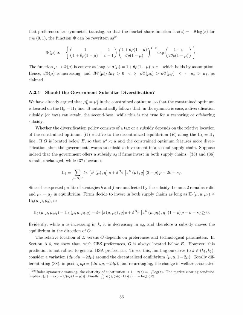
that preferences are symmetric translog, so that the market share function is s(z) = −θ log(z) for

z ∈ (0, 1), the function Φ can be rewritten as23

Φ (µ) ∝ −

(1

1 + θρ(1− µ)+

1

ε− 1

)(1 + θρ(1− µ)

θρ(1− µ)

)1−εexp

(1− ε

2θρ(1− µ)

).

The function µ→ Φ(µ) is convex as long as σ(µ) = 1 + θρ(1−µ) > ε – which holds by assumption.

Hence, dΦ(µ) is increasing, and dW (µµµ)/dµf > 0 ⇐⇒ dΦ(µh) > dΦ(µf ) ⇐⇒ µh > µf , as

claimed.

A.2.1 Should the Government Subsidize Diversification?

We have already argued that µoh = µof in the constrained optimum, so that the constrained optimum

is located on the Πh = Πf line. It automatically follows that, in the symmetric case, a diversification

subsidy (or tax) can attain the second-best, while this is not true for a reshoring or offshoring

subsidy.

Whether the diversification policy consists of a tax or a subsidy depends on the relative location

of the constrained optimum (O) relative to the decentralized equilibrium (E) along the Πh = Πf

line. If O is located below E, so that µo < µ and the constrained optimum features more diver-

sification, then the governments wants to subsidize investment in a second supply chain. Suppose

indeed that the government offers a subsidy sd if firms invest in both supply chains. (35) and (36)

remain unchanged, while (37) becomes

Πb =∑j=H,F

δπ[zj (µ) , q

]ρ+ δBπ

[zB (µ) , q

](2− ρ) ρ− 2k + sd.

Since the expected profits of strategies h and f are unaffected by the subsidy, Lemma 2 remains valid

and µh = µf in equilibrium. Firms decide to invest in both supply chains as long as Πb(µ, µ, µb) ≥Πh(µ, µ, µb), or

Πb (µ, µ, µb,q)−Πh (µ, µ, µb,q) = δπ [z (µ, µb) , q] ρ+ δBπ[zB (µ, µb) , q

](1− ρ) ρ− k + sd ≥ 0.

Evidently, while µ is increasing in k, it is decreasing in sd, and therefore a subsidy moves the

equilibrium in the direction of O.

The relative location of E versus O depends on preferences and technological parameters. In

Section A.4, we show that, with CES preferences, O is always located below E. However, this

prediction is not robust to general HSA preferences. To see this, limiting ourselves to k ∈ (k1, k2),

consider a variation (dµ, dµ,−2dµ) around the decentralized equilibrium (µ, µ, 1− 2µ). Totally dif-

ferentiating (38), imposing dµµµ = (dµ, dµ,−2dµ), and re-arranging, the change in welfare associated

23Under symmetric translog, the elasticity of substitution is 1 − σ(z) = 1/ log(z). The market clearing conditionimplies z(µ) = exp[−1/(θρ(1− µ))]. Finally,

∫ 1

zs(ζ)/ζ dζ · 1/s(z) = − log(z)/2.

36

with this variation is

−1

2

dW (µ, µ)

dµ= δ

([ε− 1

σ[z(µ)]+ 1

]P ′[z(µ)]

P [z(µ)]+σ′[z(µ)]

σ[z(µ)]2

)P [z(µ)]1−ε

∂z(µ)

∂µ+

δB([

ε− 1

σ[zB(µ)]+ 1

]P ′[zB(µ)]

P [zB(µ)]+σ′[zB(µ)]

σ[zB(µ)]2

)P [zB(µ)]1−ε

∂zB(µ)

∂µ− k,

(39)

where, as before, z(µ) := zJ(µ, µ, 1 − 2µ) for J ∈ H,F and zB(µ) := zB(µ, µ, 1 − 2µ). Charac-

terizing the sign of dW for general HSA preferences is complicated; however, this is feasible under

symmetric translog preferences. Assuming σ(z) = 1− 1/ log(z) for z ∈ (0, 1), the change in welfare

becomes

−1

2

dW (µ, µ)

dµ=

(1

2+

ε(1 + 3θn(µ))

2θn(µ)(1 + θn(µ))

)δ

1 + θn(µ)

ρθ

θnP [z(µ)]1−ε+(

1

2+

ε(1 + 3θnB(µ))

2θnB(µ)(1 + θnB(µ))

)δB

1 + θnB(µ)

ρ(1− ρ)θ

θnB(µ)P [zB(µ)]1−ε − k.

Since k ∈ (k1, k2), we have µ ∈ (0, 1/2), and the condition Π(µ, µ, 1− 2µ) = Πb(µ, µ, 1− 2µ) holds

in the decentralized equilibrium. Solving for k in Π(µ, µ, 1 − 2µ) = Πb(µ, µ, 1 − 2µ) and plugging

its value in the above equation yields

dW (µ, µ)

dµ=

(1− ε(1 + 3θn(µ))

θn(µ)(1 + θn(µ))

)δ

1 + θn(µ)

ρθ

θn(µ)P [z(µ)]1−ε+(

1− ε(1 + 3θnB(µ))

θnB(µ)(1 + θnB(µ))

)δB

1 + θnB(µ)

ρ(1− ρ)θ

θnB(µ)P [zB(µ)]1−ε.

The terms in parenthesis are increasing in n(µ) and nB(µ) respectively. Furthermore, n(µ) =

ρ(1− µ) < ρ(1 + (1− ρ)(1− 2µ)) = nB(µ). Therefore, if the first term is positive, so is the second,

and it follows that

θn(µ)(1 + θn(µ))

1 + 3θn(µ)> ε ⇒ dW (µ, µ)

dµ

∣∣∣∣µ=µo

> 0.

Alternatively, if the second term is negative, so is the first, and

θnB(µ)(1 + θnB(µ))

1 + 3θnB(µ)< ε ⇒ dW (µ, µ)

dµ

∣∣∣∣µ=µo

< 0.

We summarize this findings in the following lemma.

Lemma 3 Suppose countries are symmetric, γF = γH and qF = qH , and preferences are symmetric

translog. Then, E lies below O if

η(µ) :=θn(µ)(1 + θn(µ))

1 + 3θn(µ)> ε, (40)

37

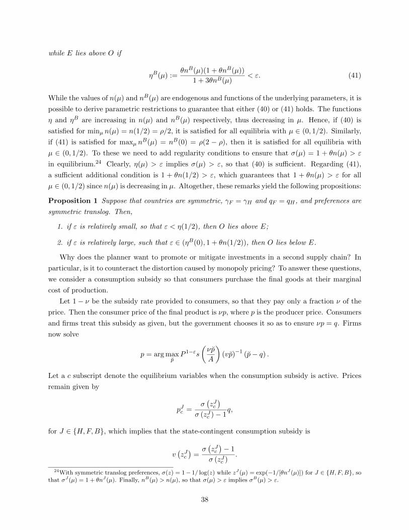
while E lies above O if

ηB(µ) :=θnB(µ)(1 + θnB(µ))

1 + 3θnB(µ)< ε. (41)

While the values of n(µ) and nB(µ) are endogenous and functions of the underlying parameters, it is

possible to derive parametric restrictions to guarantee that either (40) or (41) holds. The functions

η and ηB are increasing in n(µ) and nB(µ) respectively, thus decreasing in µ. Hence, if (40) is

satisfied for minµ n(µ) = n(1/2) = ρ/2, it is satisfied for all equilibria with µ ∈ (0, 1/2). Similarly,

if (41) is satisfied for maxµ nB(µ) = nB(0) = ρ(2 − ρ), then it is satisfied for all equilibria with

µ ∈ (0, 1/2). To these we need to add regularity conditions to ensure that σ(µ) = 1 + θn(µ) > ε

in equilibrium.24 Clearly, η(µ) > ε implies σ(µ) > ε, so that (40) is sufficient. Regarding (41),

a sufficient additional condition is 1 + θn(1/2) > ε, which guarantees that 1 + θn(µ) > ε for all

µ ∈ (0, 1/2) since n(µ) is decreasing in µ. Altogether, these remarks yield the following propositions:

Proposition 1 Suppose that countries are symmetric, γF = γH and qF = qH , and preferences are

symmetric translog. Then,

1. if ε is relatively small, so that ε < η(1/2), then O lies above E;

2. if ε is relatively large, such that ε ∈ (ηB(0), 1 + θn(1/2)), then O lies below E.

Why does the planner want to promote or mitigate investments in a second supply chain? In

particular, is it to counteract the distortion caused by monopoly pricing? To answer these questions,

we consider a consumption subsidy so that consumers purchase the final goods at their marginal

cost of production.

Let 1− ν be the subsidy rate provided to consumers, so that they pay only a fraction ν of the

price. Then the consumer price of the final product is νp, where p is the producer price. Consumers

and firms treat this subsidy as given, but the government chooses it so as to ensure νp = q. Firms

now solve

p = arg maxpP 1−εs

(νp

A

)(vp)−1 (p− q) .

Let a c subscript denote the equilibrium variables when the consumption subsidy is active. Prices

remain given by

pJc =σ(zJc)

σ (zJc )− 1q,

for J ∈ H,F,B, which implies that the state-contingent consumption subsidy is

v(zJc)

=σ(zJc)− 1

σ (zJc ).

24With symmetric translog preferences, σ(z) = 1− 1/ log(z) while zJ(µ) = exp(−1/[θnJ(µ)]) for J ∈ H,F,B, sothat σJ(µ) = 1 + θnJ(µ). Finally, nB(µ) > n(µ), so that σ(µ) > ε implies σB(µ) > ε.

38

Regardless of the presence of a consumption subsidy, the market clearing conditions remain iden-

tical, n(µµµ)s[zJc (µµµ)] = 1 for j ∈ H,F,B, and therefore zJc (µ) = zJ(µµµ). However, the price index

and the profit per state expressions are changed. Specifically, the price index becomes

logPc[zJ(µµµ)] = CP + log

q

zJ(µµµ)− 1

s[zJ(µµµ)]

∫ z

zJ (µµµ)

s (ζ)

ζdζ, (42)

and profits per state update to

π[zJ(µµµ)

]:=

s[zJ(µµµ)]

σ[zJ(µµµ)]− 1Pc[z

J(µµµ)]1−ε. (43)

The expressions for expected profits remain qualitatively as before. Hence, there still exists k1,c

and k2,c so that µh, µf , µb ∈ (0, 1) and µb = 1− µh − µf for k ∈ (k1,c, k2,c). As before, we focus on

this interior case. The expression for welfare needs now to account for the fact that the government

pays out consumption subsidies in the amount 1−νν P 1−ε

c .25 Since v (z) = σ(z)−1σ(z) , the consumption

subsidy bill equals 1σ(z)−1P

1−εc , and welfare – under the assumption that µh + µf ∈ (0, 1) – reads

W (µh, µf ) =∑

J=H,F,B

δJnJ(µµµ)πJ [zJ(µµµ)] +∑

J=H,F,B

δJ(

1

ε− 1− 1

σ[zJ(µµµ)]− 1

)Pc[z

J(µ)]1−ε − k(2− µh+f ).

Plugging (43) into the welfare expression gives

W (µh, µf ) =1

ε− 1

∑J=H,F,B

δJPc[zJ(µµµ)]1−ε − k(2− µh+f ).

The first-best allocation is obtained by maximizing the above function over (µh, µf ). As in the case

without consumption subsidy, it is evident that µh = µf =: µ satisfies the first-order conditions due

to the symmetry. We therefore focus on the case with µh = µf . Starting from the decentralized

equilibrium, µµµ, consider a deviation (dµ, dµ,−2dµ). The change in welfare associated with this

variation is

−1

2

dW (µ, µ)

dµ= δρ

∫z(µ)

s(ζ)

ζdζP [zc(µ)]1−ε + δBρ(1− ρ)

∫zB(µ)

s(ζ)

ζdζP [zBc (µ)]1−ε − k.

Considering only interior equilibrium, it must be that Π = Πb. Solving for k and plugging in the

25Total consumer spending is νpxn while the firms collect pxn. Therefore the government’s subsidy bill is

(1− ν) pxn =1− νν

vpxn =1− νν

P 1−ε.

39

above equation becomes

1

2

dW (µ, µ)

dµ= δρ

(s[z(µ)]

σ[z(µ)]− 1−∫z(µ)

s(ζ)

ζdζ

)P [zc(µ)]1−ε+

δBρ(1− ρ)

(s[zB(µ)]

σ[zB(µ)]− 1−∫zB(µ)

s(ζ)

ζdζ

)P [zBc (µ)]1−ε.

Evidently, dW (µ, µ) > 0 if and only if

s(z)

σ (z)− 1>

∫ z

z

s (ζ)

ζdζ,

for z ∈ z(µ), zB(µ), which is necessarily the case when the elasticity σ (z) is increasing in z; i.e.,

Marshall’s Second Law of Demand is satisfied. In the CES case, in which this elasticity is constant,

dW (µ?, µ?) = 0. We therefore conclude this section with the following proposition.

Proposition 2 Suppose that countries are symmetric, γF = γH and qF = qH . Suppose, in addi-

tion, that consumption subsidies equate prices to the marginal cost of production. Then, if σ′(z) > 0,

the first-best features less investment in a second supply chain. If σ′(z) = 0 (CES), the first-best is

attained with consumption subsidies alone.

A.2.2 Should the Government Subsidize Reshoring or Offshoring?

How does the sign of a reshoring (or offshoring) subsidy relate to that of the diversification subsidy?

To answer, this question, let sr denote the subsidy on the home supply chain. Intuitively, a subsidy

on the home supply chain increases the fraction of firms that invest in country H, that is it increases

µh and µb, while it decreases the fraction of firm that invests in the foreign country alone, µf . To see

this, note that the three equations that pin down an interior equilibrium are now Πb(µµµ) = Πh(µµµ),

Πh(µµµ) + sr = Πf (µµµ) and µb = 1− µh+f , or using (35-37)

δρπ[zF (µh)] + δBρ(1− ρ)π[zB(µh+f )]− k = 0,

δρπ[zF (µh)]− δρπ[zH(µf )]− sr = 0.

Using the implicit function theorem,(∂µh/∂sr

∂µf/∂sr

)=

1

∆

(−δBρ(1− ρ)dπ[zB(µh+f ])

δρdπ[zF (µh)] + δBρ(1− ρ)dπ[zB(µh+f ])

),

where

∆ := −ρ2δdπ[zH(µf )] ·δdπ[zF (µh)] + δB(1− ρ)dπ[zB(µh+f )]

−

ρ2δB(1− ρ)dπ[zB(µh+f )] · δdπ[zF (µh)] < 0.

40

Using dµb = −dµh+f , we conclude that

∂µh∂sr

= −ρ(1− ρ)

∆δBdπ[zB(µh+f )]

dµh+f> 0,

∂µb∂sr

= − ρ∆δdπ[zF (µh)]

dµh> 0,

∂µf∂sr

= −(∂µb∂sr

+∂µh∂sr

)< 0.

With this in mind, we can now proceed to show that a reshoring subsidy is welfare-improving if

and only if the second-best equilibrium features a larger degree of diversification; that is, if and

only if O is below E. When the government offers a subsidy to the home supply chain, it pays

out sr(µh + µb) = sr(1− µf ) to firms and collect taxes on households of the same amount. Hence,

the welfare expression (38) remains unchanged. Suppose now that, starting from sr = 0, the

government increases the subsidy on the home supply chain by dsr > 0. The change in welfare

associated with this variation reads

dW (µh, µf )

dsr

∣∣∣∣sr=0

/∂µb∂sr

= δ

([ε− 1

σ[z(µ)]+ 1

]P ′[z(µ)]

P [z(µ)]+σ′[z(µ)]

σ[z(µ)]2

)P [z(µ)]1−ε

∂z(µ)

∂µ+

+ δB([

ε− 1

σ[zB(µ)]+ 1

]P ′[zB(µ)]

P [zB(µ)]+σ′[zB(µ)]

σ[zB(µ)]2

)P [zB(µ)]1−ε

∂zB(µ)

∂µ− k,

where we used the fact that, when sr = 0, µh = µf = µ and µb = 1−2µ, as well as dµf+dµh = −dµb.Comparing with (39), we immediately see that

dW (µh, µf )

dsr

∣∣∣∣sr=0

/∂µb∂sr

= −1

2

dW (µ, µ)

dµ,

and therefore, since µb is increasing in sr,

dW (µh, µf )

dsr

∣∣∣∣sr=0

> 0 ⇐⇒ dW (µ, µ)

dµ.

That is, a subsidy on the home supply chain increases welfare only if the constrained optimum

features more diversification, as claimed.

A.3 The Asymmetric Case

We now return to the general model described in Section A.1. When qF < qH , Lemma 1 no

longer applies in state B since firms are not indifferent where to source from. We therefore start

by extending Lemma 1 to functions πB,H(µµµ) and πB,F (µµµ). In terms of notation, we omit the

dependence of the variables on qqq since we keep those costs constant.

We first show that, since qF < qH , prices of the goods produced with inputs from country F

must be strictly cheaper in state B than goods produced with inputs from country H. Suppose

41

not, so that pB,F ≥ pB,H . From the pricing equation (6), we have

pB,H =σ(pB,H/AB)

σ(pB,H/AB)− 1qH ≤

σ(pB,F /AB)

σ(pB,F /AB)− 1qF = pB,F <

σ(pB,F /AB)

σ(pB,F /AB)− 1qH .

However, the mark-up σ/(σ − 1) is (weakly) increasing in p, contradicting the strict inequality

above. Hence, for any allocation µµµ, we have zB,H(µµµ) > zB,F (µµµ), and firms supplying from the

low-cost country make higher profits than firms supplying from the high-cost country in state B.26

Lemma 4 If qF < qH , then zB,F (µµµ) < zB,H(µµµ) and πB,F (µµµ) > πB,H(µµµ) for all µµµ.

To show that πB,i(µµµ) is increasing in (µh, µf ), we start by studying the response of profits to

changes in the number of products available, nB,H and nB,F . To keep the notation succinct, we

omit the dependence of the variables on µµµ. In equilibrium, relative prices and the price aggregator

are jointly determined by

pB,J =σ(pB,J/AB

)σ (pB,J/AB)− 1

qJ , J ∈ H,F

1 =∑

J=H,F

nB,Js(pB,J/AB

).

For the rest of the proof, define σB,J := σ(pB,J/AB) and similarly for the other variables. For

a proportional variation (nB,H , nB,F ) in the number of active supply chains in country H and F

respectively, the proportional change in prices read27

pB,J = −αJ∆

∑`=H,F

nB,`sB,`nB,` < 0,

for J ∈ H,F, and the proportional change in the price aggregator is

AB = − 1

∆

∑J=H,F

nB,JsB,J nB,J < 0,

where we defined

αJ :=ηB,Jσ

σB,J − 1 + ηB,Jσ

∈ (0, 1) ; ∆ :=2∑

J=H,F

(1− αJ)nB,JsB,J(σB,J − 1

)> 0, (44)

for ησ := σ′ · z/σ the elasticity of σ at z. These imply that raising the number of firms reduces

26Recall that πB,i(µ) = s(zB,i)/σ(zB,i) · (PB)1−ε. Since z → s(z)/σ(z) is increasing and PB is constant across i’s,it automatically follows that πB,F > πB,H .

27x := dx/x denote the proportional change in x.

42

prices and reduces the aggregator. Furthermore,

zJ := pJ − AB =1− αJ

∆

∑`=H,F

nB,`sB,`nB,` > 0, J ∈ H,F.

It follows that the market share of every firm declines in the number of active firms and its elasticity

of demand rises, thereby reducing markups. Moving on to the price index, we start by noting that

the price index elasticity is negative,28

∂ logPB

∂ log nB,I= −n

B,IsB,I

∆

∑`=H,F

nB,`sB,`α` − nB,I∫ z

pB,I/A

s (ζ)

ζdζ < 0,

for I ∈ H,F. Therefore, the profit elasticity reads

∆

nB,IsB,I(ε− 1)

∂ log πB,J

∂ log nB,I= −

(σB,J − 1

ε− 1

)+∑`=H,F

nB,`sB,`α` +∆

sB,I

∫ z

pB,I/A

s (ζ)

ζdζ, (45)

for I, J ∈ H,F. Clearly, if ε < 1, then the elasticity is negative for both I and J . Otherwise,

recall that

1

s(z)

∫ z

z

s (ζ)

ζdζ <

1

σ (z)− 1,

such that, using the definition of ∆, we have

∆

nB,IsB,I(ε− 1)

∂ log πB,J

∂ log nB,I≤ −

(σB,J − 1

ε− 1

)+∑`=H,F

nB,`sB,`(α` + (1− αl)

σB,` − 1

σB,I − 1

).

Since zB,H > zB,F , we have σB,H ≥ σB,F > ε, and therefore

σB,H − 1

ε− 1≥ σB,` − 1

ε− 1>σB,` − 1

σB,i − 1,

for `, i ∈ H,L. It follows that the elasticity of πB,H is decreasing with both nB,H and nB,F .

Similarly,

σB,F − 1

ε− 1> 1 ≥ σB,` − 1

σB,H − 1,

and πB,F is decreasing with nB,H . It is harder to sign the elasticity of πB,F with respect to nB,F .

28Recall that the price index reads

logPB = CP + logAB −∑i=H,F

nB,i∫ z

pB,i/AB

s(ζ)

ζdζ

43

However, note that when qF → qH , we have σB,F → σB,H , and therefore

∆

nB,IsB,I(ε− 1)

∂ log πB,J

∂ log nB,I≤ −σ

B − εε− 1

< 0.

for I, J ∈ H,F. Furthermore, in the CES case, we have αJ = 0 for both J , and therefore

∆

nB,IsB,I(ε− 1)

∂ log πB,J

∂ log nB,I= −

(σ − εε− 1

)< 0.

We summarize these results in the following lemma.

Lemma 5 Suppose that qF < qH . Then, πB,H is decreasing in both nB,F and nB,H . Similarly,

πB,F is decreasing in nB,H . Finally, if qF ≈ qH or preferences are CES, then πB,F is also decreasing

in nB,F .

For the differential costs used in the numerical simulations, qF /qH ∈ [0.8, 1], we found Lemma 5

to always hold. From Lemma 5, it is possible to draw conclusions about the relationship between

firm investment and profits. From (24) and (25), it is immediate that πB,J is increasing in µf for

J ∈ H,F.

Corollary 1 Suppose that qF < qH but γF = γH . Then, πB,F and πB,H are increasing in µf .

Regarding the impact of µh on profits, we have

∂ log πB,J

∂µh= ρ

(∂ log πB,J

∂nB,Hρ− ∂ log πB,J

∂nB,F

).

Using (45),

∂ log πB,J

∂µh∝(sB,F − ρsB,H

)(σB,J − 1

ε− 1

)−∑`=H,F

nB,`sB,`α`

−∆

(∫ z

pB,F /A

s (ζ)

ζdζ − ρ

∫ z

pB,H/A

s (ζ)

ζdζ

),

(46)

for J ∈ H,F, where the constant of proportionality is identical across the J ’s. The elasticity of

πB,H can be signed. Since zB,H > zB,F , we have σB,H > σB,F , and therefore

[∫zB,F

s(ζ)

ζdζ − ρ

∫zB,H

s(ζ)

ζdζ

]∆ <

(∫ zB,H

zB,F

s(ζ)

ζdζ + (1− ρ)

∫zB,H

s(ζ)

ζdζ

)(σB,H − 1

)1−∑`=H,F

nB,`sB,`α`

<

(sB,F − sB,H

σB,F − 1+ (1− ρ)

sB,H

σB,H − 1

)(σB,H − 1

)1−∑`=H,F

nB,`sB,`α`

< (sB,F − ρsB,H)

σB,H − 1

σB,F − 1

1−∑`=H,F

nB,`sB,`α`

,

44

where the first inequality follows from the definition of ∆ (44), σB,H > σB,F and the market clearing

condition∑

`=H,F nB,`sB,` = 1, the second from (23), and the last inequality from σB,H > σB,F

again. Combined with (σB,H − 1)/(σB,F − 1) > (σB,H − 1)/(ε− 1), this is sufficient to show that

πB,H is increasing with µh. Signing the elasticity of πB,F is trickier. However, when qF → qH , the

elasticity simplifies to

∂ log πB,J

∂µh∝ sB

(σB − 1

ε− 1− α

)− (1− α)(σB − 1)

∫ z

pB/A

s (ζ)

ζdζ ≥ sB

(σB − εε− 1

)> 0,

for both J ∈ H,F since firms become indifferent between the location of their supply chain.

Alternatively, when preferences are CES,

∂ log πB,J

∂µh∝(sB,F − ρsB,H

)(σ − εε− 1

)≥ 0,

where we used∫z s(ζ)/ζdζ = s(z)/(σ − 1), αJ = 0 and ∆ = σ − 1 under CES preferences.

Corollary 2 Suppose that qF < qH but γF = γH . Then, πB,H is increasing in µh. If qF ≈ qH or

preferences are CES, then πB,F is also increasing in µh.

The profit semi-elasticity (46) is also useful to show that the following assumption – which we

need to establish the configuration depicted in Figure 3 when qF < qH – is met under qF ≈ qH .

Assumption 3 The function Πfh(µh, µf ) := Πf (µh, µf , 1 − µh − µf ) − Πh(µh, µf , 1 − µh − µf )

satisfies

∂Πfh(µh, µf )

∂µf< 0 ;

∂Πfh(µh, µf )

∂µh> 0.

We proceed to show that this assumption is met when qF ≈ qH . Using the expressions for profits

per state, the function of interest is Πfh(µµµ)/ρ = δFπ[zF (µµµ), qF ] − δHπ[zH(µµµ), qH ] + δB[πB,F (µµµ) −πB,H(µµµ)]. Since zF is solely a function of µh, we have

∂Πfh(µh, µf )

∂µf∝ −δH dπ[zH(µµµ), qH ]

dµf− δB

(∂πB,F (µµµ)

∂µf− ∂πB,H(µµµ)

∂µf

).

From (45), it is easy to see that ∂(πB,F − πB,H)/∂nB,H → 0 as qF → qH . Since the first term is

strictly negative, this guarantees that Πfh is decreasing in µf for qF ≈ qH . Similarly, since zH is

independent of µh, we have

∂Πfh(µh, µf )

∂µh∝ δF dπ[zF (µµµ), qF ]

dµh+ δB

(∂πB,F (µµµ)

∂µh− ∂πB,H(µµµ)

∂µh

).

From the expression for ∂ log πB,i/∂µh, it is also easy to see that ∂(πB,F − πB,H)/∂µh → 0 for

qF → qH , and therefore Πfh is increasing in µh.

45

We can now move to proving Figure 3.29 For that, we proceed in two ways. First, we analyze an

economy with γF < γH but qF = qH . When that is the case, firms remain indifferent between the

two countries in state B and there is a unique price, zB, allowing us to re-use most of the results

of Section A.2. The proof is by construction, and does not require Assumption 3.

Since country H is safer and offers the same marginal cost, relatively more firms want to settle

a supply chain there than in country F . To see this, suppose the contrary: firms invest relatively

more in the risky country, µf > 0 and µf ≥ µh. From the market clearing conditions, we then have

s[zF (µµµ)] =1

ρ(µf + µb)≤ 1

ρ(µh + µb)= s[zH(µµµ)].

Since z → s(z) is decreasing, it must be that zH(µµµ) ≤ zF (µµµ). But z → π(z) is decreasing, so

that δFπ[zF (µµµ)) ≤ δFπ[zH(µµµ)] < δHπ[zH(µµµ)]. However, this in turn implies that the expected

profits of the foreign strategy are lower, Πf < Πh, and therefore µf = 0, a contradiction. Hence,

in equilibrium, it must either be that no firms invest in the risky country, µf = 0, or if some firms

do, relatively more firms need to invest in the safe country, µf > 0 and µh > µf . Accordingly, it

must also be that the expected profits of the safer strategy are (weakly) higher than the expected

profits of the less safe strategy, Πh ≥ Πf .

Given that the expected profits of the home supply chain are weakly higher than those with a

supplier in the foreign country, firms’ investments are dictated by two comparisons: home versus

foreign supply chains, Πh(µh, µf , µb) − Πf (µh, µf , µb), and single supply chain at home versus

diversification, Πh(µh, µf , µb) − Πb(µh, µf , µb).30 Using the expressions for expected profits, these

two optimality conditions respectively read

Πh(µh, µf , µb) ≥ Πf (µh, µf , µb) ⇐⇒ δHπ[zH(µh, µf , µb)] ≥ δFπ[zF (µh, µf , µb)],

and

Πb(µh, µf , µb) ≥ Πh(µh, µf , µb) ⇐⇒ δFπ[zF (µh, µf , µb)] + δBρ(1− ρ)π[zB(µh, µf , µb)] ≥ k.

In addition, profits must be positive, Πj(µh, µf , µb) ≥ 0 for j ∈ h, f, b.For k 0, investing in resilience is clearly the most profitable option, Πb > Πh > Πf , where the

second inequality follows from δHπ[zH(0, 0, 1)] > δFπ[zF (0, 0, 1)]. Hence, for low k, µh = 0 = µf

and µb = 1. As the fixed cost increases, the gap between Πh(0, 0, 1) − Πb(0, 0, 1) shrinks to the

point where the two strategies yield the same expected profits. This occurs at k1, defined by

k1 := δFρπ[zF (0, 0, 1)] + δBρ(1− ρ)π[zB(0, 0, 1)].

At k = k1, we thus have Πb(0, 0, 1) = Πh(0, 0, 1) > Πf (0, 0, 1). For µh ∈ [0, 1], there always exists

29For both proofs we assume that CP is small enough so that we do not have to check Πj < 0 until k > k4.30Without Πh ≥ Πf , we would also need to compare Πf −Πb.

46

a k > k1 that ensures Πb(µh, 0, 1− µh) = Πh(µh, 0, 1− µh), defined by31

κ2(µh) := δFρπ[zF (µh, 0, 1− µh)] + δBρ(1− ρ)π[zB(µh, 0, 1− µh)],

with κ2(0) = k1. As in Section A.2, π[zF (µµµ)] and π[zB(µµµ)] are increasing in µh, and therefore

so is κ2(µh).32 Let µ2h(k) denote the inverse of κ2(µh). The allocation (µ2

h(k), 0, 1 − µ2h(k)) is an

equilibrium if and only if Πh(µh(k), 0, 1−µh(k)) > Πf (µh(k), 0, 1−µh(k)). The difference between

the two expected profits can be rewritten as

Πh(µh, 0, 1− µh)−Πf (µh, 0, 1− µh) = δHρπ[zH(µh, 0, 1− µh)]− δFρπ[zF (µh, 0, 1− µh)].

When µf = 0, zH is obtained from ρs[zH(µµµ)] = 1, so that zH is constant. Hence, Πh − Πf is

monotonically decreasing in µh. There are therefore two cases. If Πh(1, 0, 0) ≥ Πf (1, 0, 0), then

that is also the case for all µh ∈ [0, 1], and the allocation (µh(k), 0, 1− µh(k)) is an equilibrium for

all k ∈ (k1, k2), where k2 := κ2(1). On the contrary, if Πh(1, 0, 0) < Πf (1, 0, 0), then there exists a

µh ∈ (0, 1) for which Πh(µh, 0, 1−µh) = Πf (µh, 0, 1−µh) and Πh(µh, 0, 1−µh) > Πf (µh, 0, 1−µh) for

µh < µh. In that case, (µh(k), 0, 1−µh(k)) is an equilibrium for all k ∈ (k1, k2), where k2 := κ2(µh),

but not for k > k2. In both cases, µh is increasing with k.

Focusing on the second case, at k = k2 the three strategies yield the same expected profits. For

µ > µh(k2), define the function µf (µh) that ensures equiprofitability between the home and foreign

supply; specifically, let the function µf (µh) satisfy

δFπ[zF (µh, µf (µh), 1− µh − µf (µh))] = δHπ[zH(µh, µf (µh), 1− µh − µf (µh))]. (47)

The monotonicity of µ → π[z(µ)] ensures that µh → µf (µh) is well-defined for all µh so that

µh + µf (µh) ≤ 1 and is increasing. Abusing the notation, let µh be such that µh + µf (µh) = 1.

Meanwhile, to guarantee that (µh, µf (µh), 1−µh−µf (µh)) is an equilibrium, we also need to ensure

indifference between the home supply chain and the diversification strategy. This is guaranteed by

appropriately adjusting the fixed cost; specifically, define κ3(µh) on µh ∈ (µh(k2), µh) by

κ3(µh) := δFρπ[zF (µh, µf (µh), 1− µh − µf (µh))] + δBρ(1− ρ)π[zB(µh, µf (µh), 1− µh − µf (µh))].

Both π(zF ) and π(zB) are increasing in µh, and therefore so is κ3(µh).33 Let k3 := κ3(µh) and

µ3h(k) denote the inverse function of κ3(µh). By construction, the allocation (µh(k), µf [µh(k)], 1−µh(k)− µf [µh(k)]) is thus an equilibrium for all k in (k2, k3), with both µh and µf increasing with

k.

31For any µh ∈ [0, 1], we have π[zj(µh, 0, 1 − µh)] < ∞. Hence, Πh − Πb < 0 for k 0, Πh − Πb > 0 for k 0,and Πh −Πb is monotonically increasing in k.

32The market clearing conditions are (1− µh)ρs[zF (µµµ)] = 1 and ρ[1 + (1− ρ)(1− µh)]s[zB(µµµ)] = 1, from which itfollows that zF and zB are decreasing in µh. The monotonicity of µ→ π[z(µ)] then follows from Lemma 1.

33This again follows from the market clearing conditions and Lemma 1, which together ensures that π[zF (µµµ)] is anincreasing function of µf + µh.

47

At k = k3, firms are indifferent between the three strategies, and Πh(µh, 1− µh, 0) = Πf (µh, 1−µh, 0) = Πb(µh, 1 − µh, 0). For any k > k3, investing in both supply chains is no longer the most

profitable strategy, so that Πh(µh, 1− µh, 0) = Πf (µh, 1− µh, 0) > Πb(µh, 1− µh, 0). The allocation

(µh, 1 − µh, 0) therefore constitutes an equilibrium for k ≥ k3 as long as Πh(µh, 1 − µh, 0) =

Πf (µh, 1 − µh, 0) ≥ 0. Let k4 denote the level of fixed cost that make firms indifferent between

investing in either supply chain or exiting,

k4 := δHρπ[zH(µh, 1− µh, 0)] + δBρπ[zB(µh, 1− µh, 0)]

Clearly, for any k > k4, Πh(µh, 1 − µh, 0) = Πf (µh, 1 − µh, 0) < 0, and therefore (µh, 1 − µh, 0) is

no longer an equilibrium. Instead, with a slight abuse of notation, let µf (µh) denote the function

that guarantees the equiprofitability between the home and foreign supply chain when µb = 0,34

δFπ[zF (µh, µf (µh), 0)] = δHπ[zH(µh, µf (µh), 0)].

The functions zH and zF are obtained from the market clearing conditions ρµhs[zH(µµµ)] = 1 and

ρµfs[zF (µµµ)] = 1 respectively, so that zH is increasing in µh and zF is increasing in µf . Jointly with

Lemma 1, this guarantees that the function µf (µh) is well defined as long as µf (µh) ≥ 0 and µf is

increasing in µh. If limµ→0 π[z(µ, µ, 0)] = ∞, then µf is well-defined on (0, µh). Otherwise, since

δFπ[zF (0, 0, 0)] < δHπ[zH(0, 0, 0)], it must be that δFπ[zF (µh, 0, 0)] = δHπ[zH(µ

h, 0, 0)] for some

µh> 0.

Given that, by construction, firms are indifferent between the home and foreign supply chain,

(µh, µf (µh), 0) constitutes an equilibrium for k > k4 if and only if (1) profits are weakly positive,

and (2) investing in both places is not more profitable. To satisfy the first condition, adjust the

fixed cost so as to ensure Πh = 035

κ5(µh) = δHρπ[zH(µh, µf (µh), 0)] + δBρπ[zB(µh, µf (µh), 0)],

for all µh ∈ (µh, µh). We already know that π[zH(µµµ)] is decreasing in µh. Meanwhile, the function

zB is given by ρ(µf + µh)s[zB(µµµ)], so that zB is increasing in µh, and π[zB(µh, µf (µh), 0)] is

decreasing in µh. Together, these imply that κ5 is decreasing in µh on (µh, µh), or said differently,

µh is increasing in k for k ∈ (k4, k5), where k5 := κ5(µh). Regarding the second condition, the

expected profits of the diversification strategy can be written as Πb = Πh + Πf − δBρ2π(zB), such

that Πh = Πf = 0 implies Πb < 0 and no firm wants to invest in both supply chains. As before, let

µ5h(k) denote the inverse of k(µh). For k ∈ (k4, k5), the allocation (µh(k), µf [µf (k)], 0) is therefore

an equilibrium, and both µh and µf are decreasing in k.36

34Note that this function is different from the one defined in (47) precisely because µb = 0.35Note that Πh(µh, µf (µh), 0) = δHρπ[zH(µh, µf (µh), 0)] + δBρ(1− ρ)π[zB(µh, µf (µh), 0)]− k is decreasing in µh.

Since Πh(µh, 1− µh, 0) = 0 at k4, it simply cannot be that, in equilibrium, Πh > 0 for k > k4.36Note that, if µ

h= 0, then k5 =∞.

48

Finally, for k > k5, the equilibrium consists of (µh, 0, 0), where µh ensures Πh = 0, specifically

δHρπ[zH(µh, 0, 0)] + δBρπ[zB(µh, 0, 0)] = k.

The functions π[zH(µh, 0, 0)] and π[zB(µh, 0, 0)] remain decreasing in µh, so that µh decreases with

k. As for k ∈ (k4, k5), Πh = 0 ensures that Πb < 0. Furthermore, µh(k) < µh, which guarantees

that Πf < Πh. If π[z(0, 0, 0)] < ∞, there exists a final threshold k6 above which no firms want to

invest in any supply relationship,

k6 := limµh0

δHρπ[zH(µh, 0, 0)] + δBρπ[zB(µh, 0, 0)].

We now move to the second economy of interest with asymmetric marginal costs but homo-

geneous risk, qF < qH and γF = γH . The proof here is also by construction, but it requires

Assumption 3. Since the proof is similar to the proof with asymmetric risk, some steps are omit-

ted.

As always, when the fixed cost is small, it is strictly more profitable for firms to diversify their

supply chains. For larger k, firms become indifferent between diversifying their supply chains and

investing in the low-cost country only. Specifically, k1 > 0 equates Πb(0, 0, 1) = Πf (0, 0, 1) >

Πh(0, 0, 1).37

For slightly higher fixed costs, firms remain indifferent between investing in both supply chains

or in the low-cost country only, while the home-only investment remains dominated. To see this,

note that for any µf ∈ (0, 1), there exists a fixed cost k > k1 that renders firms indifferent between

strategy b and f . This fixed cost is

κ2(µf ) := δρπ[zH(0, µf , 1− µf ), qH ] + δBρ(1− ρ)πB,H(0, µf , 1− µf ).

As in the case with symmetric marginal cost, π(zH) is increasing with µf . Combined with Corol-

lary 1, this implies that κ2 is an increasing function. Let k → µ2f (k) denote the inverse of

µf → κ2(µf ), so that µ2f is increasing with k. The allocation (0, µ2

f (k), 1−µ2f (k)) is an equilibrium

if and only if Πfh(0, µ2f (k), 1−µ2

f (k)) > 0. We already know that Πfh(0, 0, 1) > 0. Furthermore, by

Assumption 3, µf → Πfh(0, µf , 1− µf ) is increasing in µf . Hence, if Πfh(0, 1, 0) < 0, there exists

a µ?f < 1 so that Πfh(0, µ?f , 1− µ?f ) = 0. Letting k2 := κ2(µ?f ), it follows that (0, µ2f (k), 1− µ2

f (k))

is an equilibrium for k ∈ (k1, k2).38

Assuming that Πfh(0, 1, 0) < 0 indeed holds, at k = k2, firms are indifferent between all three

strategies, which remains valid for higher fixed cost of investment. To see this, let µf be the (unique)

solution to Πfh(1−µf , µf , 0) = 0.39 Then, define the function µf → µh(µf ) to ensure equiprofitabil-

ity between the foreign-only and home-only supply chain, Πfh(µh(µf ), µf , 1−µh(µf )−µf ) = 0, for

37Πf (0, 0, 1) > Πh(0, 0, 1) follows from π[zF (0, 0, 1), qF ] > π[zH(0, 0, 1), qH ] and πB,F (µ) > πB,H(µ) for all µ.38As in the asymmetric risk economy, Πfh(0, 1, 0) < 0 is not necessarily satisfied. If Πfh(0, 1, 0) > 0, then

(0, µ2f (k), 1− µ2

f (k)) is an equilibrium for k ∈ (k1, k2(1)), and µh = 0 for all k.39This solution is unique because Πfh(1, 0, 0) > 0 and Πfh(0, 1, 0) < 0 while µf → Πfh(1−µf , µf , 0) is decreasing.

49

µf ∈ (µf (k2), µf ). This function is well-defined and increasing. Indeed, Πfh(0, µf (k2), 1−µf (k2)) =

0 implies that Πfh(0, µf , 1 − µf ) < 0 for all µf > µf (k2) per Assumption 3. Furthermore,

Πfh(1 − µf , µf , 0) ≥ 0 for all µf ≤ µf since µf → Πfh(1 − µf , µf , 0) ≥ 0 is decreasing. Fi-

nally, µh → Πfh(µh, µf , 1 − µh − µf ) is increasing (Assumption 3), which ensures the uniqueness

and monotonicity of µf → µh(µf ).

The allocation (µh(µf ), µf , 1 − µh(µf ) − µf ) is then an equilibrium if and only if firms are

indifferent between investing only in the low-cost country or diversifying their supply chains. This

is achieved by appropriately setting k. Specifically, define

κ3(µf ) := δρπ[zH(µh(µf ), µf , 1− µf − µh(µf )), qH ] + δBρ(1− ρ)πB,H(µh(µf ), µf , 1− µf − µh(µf )),

so as to ensure Πf = Πb along (µh(µf ), µf , 1− µf − µh(µf )). Both π(zH) and πB,H are increasing

in µf , and therefore so is κ3. Let k → µ3f (k) denote the inverse function of µf → κ3(µf ) and

k3 := κ3(µf ). Then, (µh[µf (k)], µf (k), 1−µh[µf (k)]−µf (k)) is an equilibrium for k ∈ (k2, k3), and

both µh and µf are increasing with k.

For k > k3, it automatically follows that Πj(1−µf , µf , 0) = Πf (1−µf , µf , 0) > Πb(1−µf , µf , 0),

and investing in strategy b is no longer the most profitable option. Let k4 be the fixed cost that

renders firms indifferent between existing and investing in a single-country supply chain,

k4 := δπ[zF (1− µf , µf , 0)] + δBρπB,F (1− µf , µf , 0).

The allocation (1 − µf , µf , 0) therefore constitutes an equilibrium for k ∈ (k3, k4). For k > k4,

Πj(1 − µf , µf , 0) < 0 for j ∈ h, f and some firms want to exit. Since the focus of the policy

analysis is for k ∈ (k2, k3) and the remainder of the proof for k > k3 is similar to the case with

γF < γH but qF = qH , we omit the details and move instead directly to the slopes of the iso-welfare

curves.

For the rest of this section, we focus on values of k ∈ (k2, k3) such that µh > 0, µf > 0 and

µb = 1 − µh − µf > 0. For these fixed costs, firms are indifferent among all three strategies.

The equilibrium is located at the intersection between the three functions µf → µh(µf ) defined

implicitly by Πh(µµµ) = Πf (µµµ), Πh(µµµ) = Πb(µµµ) and Πf (µµµ) = Πb(µµµ). We now proceed to show

that the curves defined by these indifference conditions have the qualitative properties shown in

Figure ??. Starting from the indifference condition between the home-only and foreign-only supply

chain, Πf −Πh = 0 implies

dµhdµf

∣∣∣∣Πf=Πh

= −∂Πfh

∂µf

/∂Πfh

∂µh> 0,

where the inequality follows from Assumption 3. Turning to the indifference between the foreign-

50

only supply chain and the diversification strategy, we have

dµhdµf

∣∣∣∣Πf=Πb

= −(

δH

1− ρdπ[zH(µf ), qH ]

dµf+∂πB,H(µµµ)

∂µf

)/∂πB,H(µµµ)

∂µh< 0,

where the inequality follows from Corollary 1 and 2. Finally, the equiprofitability of the home-only

and resilience strategy implies

dµhdµf

∣∣∣∣Πh=Πb

[δFdπ[zF (µh), qF ]

dµh+ δB

(∂πB,F (µµµ)

∂µh− ρ∂π

B,H(µµµ)

∂µh

)]= −δB

(∂πB,F (µ)

∂µf− ρ∂π

B,H(µµµ)

∂µf

).

From Assumption 3, the left hand side is positive.40 Furthermore, the right-hand side is negative if

and only if Πh −Πb = −δFπ[zF (µh), qF ]− δBρ[πB,F (µµµ)− ρπB,H(µµµ)] + k is decreasing in µf , which

we now assume.

Assumption 4 The function Πhb(µh, µf ) := Πh(µh, µf , 1 − µh − µf ) − Πb(µh, µf , 1 − µh − µf )

satisfies

∂Πhb(µh, µf )

∂µf< 0.

As with Assumption 3, this is satisfied for qF ≈ qH .41

Lastly, we want to characterize optimal policies in the world with asymmetric costs and risks.

Welfare as a function of (µoh, µof ) reads

W (µh, µf ) =∑

j=H,F,B

δjΠj(µh, µf ) +1

ε− 1

∑j=H,F

δjP [zj(µ−j)]1−ε + δBPB(µµµ)1−ε

.

Analyzing this function is complicated for general HSA preferences. However, it is possible to

extend Lemma 3 to the case where γF < γH but qF ≈ qH . Under symmetric costs, firms are

indifferent between the two countries in state B, and therefore (39) remains valid except that

µh > µf when γF < γH . In particular, under symmetric translog preferences, the change in welfare

40Indeed, ∂Πfh/∂µh > 0 writes

δFdπ[zF (µh), qF ]

dµh+ δB

(∂πB,F

∂µh− ∂πB,H

∂µh

)> 0,

and ρ ≤ 1.41We have

∂Πhb

∂µf= −δBρ

(∂πB,F (µµµ)

∂µf− ρ∂π

B,H(µµµ)

∂µf

)→ −δBρ∂π

B(µµµ)

∂µf(1− ρ) < 0.

51

caused by a variation dµµµ = (dµf , dµh) is given by

−dW (µµµ) =∑i=H,F

(1

2+

ε(1 + 3θni(µµµ))

2θni(µµµ)(1 + θni(µµµ))

)δi

1 + θni(µµµ)

ρθ

θni(µµµ)P [zi(µµµ)]1−εdµ−i+(

1

2+

ε(1 + 3θnB(µµµ))

2θnB(µµµ)(1 + θnB(µµµ))

)δB

1 + θnB(µµµ)

ρ(1− ρ)θ

θnB(µµµ)P [zB(µµµ)]1−ε

∑i

dµi − k(dµh + dµf ),

while the indifference conditions for an interior equilibrium, Πf = Πb and Πh = Πb, are

ρδHθ

θnH(µµµ)(1 + θnH(µµµ))P [zH(µµµ)]1−ε +

δBρ(1− ρ)θ

θnB(µµµ)(1 + θnB(µµµ))P [zB(µµµ)]1−ε = k,

ρδF θ

θnF (µµµ)(1 + θnF (µµµ))P [zF (µµµ)]1−ε +

δBρ(1− ρ)θ

θnB(µµµ)(1 + θnB(µµµ))P [zB(µµµ)]1−ε = k.

Combining the two,

2dW (µµµ) =∑i

(1− ε(1 + 3θni(µµµ))

θni(µµµ)(1 + θni(µµµ))

)δi

1 + θni(µµµ)

ρθ

θni(µ)P [zi(µµµ)]1−εdµ−i+(

1− ε(1 + 3θnB(µµµ))

θnB(µµµ)(1 + θnB(µµµ))

)δB

1 + θnB(µµµ)

ρ(1− ρ)θ

θnB(µµµ)P [zB(µµµ)]1−ε

∑i

dµi.

As before, the terms in parenthesis are increasing in ni(µµµ) for i ∈ H,F,B respectively. Further-

more, ni(µµµ) < nB(µµµ) for i ∈ H,F. Finally, µh > µf implies nH(µµµ) > nF (µµµ). It follows that if

the expression in parenthesis is positive for i = F , then it is positive for i ∈ H,F,B. Hence,

in this case, dW (µµµ) > 0, and increasing µf and µh – that is, reducing diversification – is welfare

improving. On the contrary, if the expression is negative for i = B, then it is negative for all J ,

and increasing diversification raises W . This allows us to extend Lemma 3.

Lemma 6 Suppose that qF = qH but γF < γH and preferences are symmetric translog. Then, O

is above E if

θnF (µµµ)(1 + θnF (µµµ))

1 + 3θnF (µµµ)> ε,

while O is below E if

θnB(µµµ)(1 + θnB(µµµ))

1 + 3θnB(µµµ)< ε.

A.4 A Special Case: CES Preferences

In this section, we focus on the limit case where the elasticity of substitution between varieties

is constant, σ′(z) = 0. The corresponding market share function is s(z) = z1−σ, where σ is the

(constant) elasticity of substitution, σ(z) = σ > ε > 0. The pricing equation yields an explicit

52

expression for prices,

pJ =

(σ

σ − 1

)qJ ,

for J ∈ H,F. In particular, prices become independent of the number of active firms and only

depend on the location where the input is produced.

In states J ∈ H,F, the market clearing condition (4) implies zJ(µµµ) = nJ(µµµ)1/(σ−1). Since

nH(µµµ) = ρ(1 − µF ), zH(µµµ) is only a function of µF . Similarly, zF (µµµ) is only a function of µh.

Imposing CP = 1/(σ − 1)− log[σ/(σ − 1)] for notational simplicity, the price index (21) simplifies

to42

P [zJ(µµµ), qJ ] =qJ

zJ(µµµ)= nJ(µµµ)

11−σ · qJ , (48)

for J ∈ H,F. As in standard trade models, the price index is decreasing in the number of

available varieties in state J , nJ(µµµ). Plugging the functional form assumption and the expression

for the price index in (22), the profit of an active firm in state J ∈ H,F becomes

π[zJ(µµµ), qJ ] =

(q1−εJ

σ

)nJ(µµµ)

ε−σσ−1 .

In state B, the price index (27) becomes a weighted geometric average of the marginal cost where

the weights are the number of active firms in each country,43

PB(µµµ) =

∑J=H,F

nB,J(µµµ)q1−σJ

11−σ

. (49)

Profits of a firm that sources in state B from country J ∈ H,F then equal

πB,J(µµµ) =

(q1−σJ

σ

) ∑`=H,F

nB,`(µµµ)q1−σ`

ε−σσ−1

.

Adapting (29) and (30), the expected profits of a firm that invests in a single-country supply

42From the market clearing condition and the pricing equation, we have A[zJ(µµµ), qJ ] = pJn(µµµ)1/(1−σ). Furthermore,from the price index (21), we also know that logP [zJ(µµµ), qJ ] − logA[zJ(µµµ), qJ ] = CP − 1/(σ − 1) when preferencesare CES. Assembling the two together and imposing the normalization on CP yields the desired expression.

43The market clearing condition implies AB(µµµ) = (∑nj(µµµ)p1−σ

j )1/(1−σ), while it remains the case under CES

preferences that logPB(µµµ)− logAB(µµµ) = CP − 1/(σ − 1). Using CP = 1/(σ − 1)− log[σ/(σ − 1)] then returns (49)

53

chain in country j ∈ h, f becomes

Πj = δj

(q1−εj

σ

)nj(µµµ)

ε−σσ−1 ρ+ δB

(q1−σj

σ

) ∑i=H,F

nB,i(µµµ)q1−σi

ε−σσ−1

ρ− k. (50)

Similarly, the expected profits of a firm that invest in both countries are

Πb =∑j=H,F

δj

(q1−εj

σ

)nj(µµµ)

ε−σσ−1 ρ+ δB

[(q1−σF

σ

)+ (1− ρ)

(q1−σH

σ

)] ∑j=H,F

nB,j(µµµ)q1−σj

ε−σσ−1

ρ− 2k.

We start by showing that, when preferences are CES, the welfare function is globally concave so

that the first-order conditions are sufficient. We focus on the case where the equilibrium is interior,

k ∈ (k2, k3). From (8), using the expressions for expected profits just derived, the market clearing

conditions s[zJ(µµµ]nJ(µµµ) = 1 and∑

J=H,F s[zB,J(µµµ]nB,J(µµµ) = 1, and the special feature of CES

that σ(z) = σ for all z, the welfare function simplifies to

W (µh, µf ) = c∑

J=H,F,B

δJP J(µµµ)1−ε − k(2− µh − µf ),

where c := 1/σ+ 1/(ε− 1). Plugging in the expression for the price indices, (48) and (49), we have

W (µh, µf ) = c

∑J=H,F

δJnJ(µµµ)1−ε1−σ q1−ε

J + δB

∑`=H,F

nB,`(µµµ)q1−σ`

1−ε1−σ− k(2− µh − µf ).

As in the general HSA preferences case, the constrained optimum is obtained by maximizing this

function over (µh, µf ); let (µoh, µof ) denote the constrained optimum. If the allocation is interior,

the constrained optimum satisfies the problem’s first-order conditions, which are

c

(1− ε1− σ

)ρ(δHnH(µµµo)

ε−σσ−1 q1−ε

H + δB(1− ρ)q1−σH PB(µµµo)σ−ε

)= k, (51)

with respect to µof , and

c

(1− ε1− σ

)ρ(δFnF (µµµo)

ε−σσ−1 q1−ε

F + δB[q1−σF − ρq1−σ

H

]PB(µµµo)σ−ε

)= k, (52)

with respect to µoh, where we used that zF is independent of µf and zH is independent of µh.

54

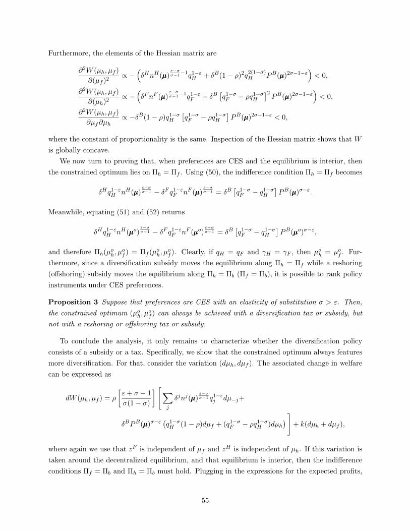
Furthermore, the elements of the Hessian matrix are

∂2W (µh, µf )

∂(µf )2∝ −

(δHnH(µµµ)

ε−σσ−1−1q1−ε

H + δB(1− ρ)2q2(1−σ)H PB(µµµ)2σ−1−ε

)< 0,

∂2W (µh, µf )

∂(µh)2∝ −

(δFnF (µµµ)

ε−σσ−1−1q1−ε

F + δB[q1−σF − ρq1−σ

H

]2PB(µµµ)2σ−1−ε

)< 0,

∂2W (µh, µf )

∂µf∂µh∝ −δB(1− ρ)q1−σ

H

[q1−σF − ρq1−σ

H

]PB(µµµ)2σ−1−ε < 0,

where the constant of proportionality is the same. Inspection of the Hessian matrix shows that W

is globally concave.

We now turn to proving that, when preferences are CES and the equilibrium is interior, then

the constrained optimum lies on Πh = Πf . Using (50), the indifference condition Πh = Πf becomes

δHq1−εH nH(µµµ)

ε−σσ−1 − δF q1−ε

F nF (µµµ)ε−σσ−1 = δB

[q1−σF − q1−σ

H

]PB(µµµ)σ−ε.

Meanwhile, equating (51) and (52) returns

δHq1−εH nH(µµµo)

ε−σσ−1 − δF q1−ε

F nF (µµµo)ε−σσ−1 = δB

[q1−σF − q1−σ

H

]PB(µµµo)σ−ε,

and therefore Πh(µoh, µof ) = Πf (µoh, µ

of ). Clearly, if qH = qF and γH = γF , then µoh = µof . Fur-

thermore, since a diversification subsidy moves the equilibrium along Πh = Πf while a reshoring

(offshoring) subsidy moves the equilibrium along Πh = Πb (Πf = Πb), it is possible to rank policy

instruments under CES preferences.

Proposition 3 Suppose that preferences are CES with an elasticity of substitution σ > ε. Then,

the constrained optimum (µoh, µof ) can always be achieved with a diversification tax or subsidy, but

not with a reshoring or offshoring tax or subsidy.

To conclude the analysis, it only remains to characterize whether the diversification policy

consists of a subsidy or a tax. Specifically, we show that the constrained optimum always features

more diversification. For that, consider the variation (dµh, dµf ). The associated change in welfare

can be expressed as

dW (µh, µf ) = ρ

[ε+ σ − 1

σ(1− σ)

] [∑j

δjnj(µµµ)ε−σσ−1 q1−ε

j dµ−j+

δBPB(µµµ)σ−ε(q1−σH (1− ρ)dµf + (q1−σ

F − ρq1−σH )dµh

) ]+ k(dµh + dµf ),

where again we use that zF is independent of µf and zH is independent of µh. If this variation is

taken around the decentralized equilibrium, and that equilibrium is interior, then the indifference

conditions Πf = Πb and Πh = Πb must hold. Plugging in the expressions for the expected profits,

55

these conditions imply

δHρ

(q1−εH

σ

)nH(µµµ)

ε−σσ−1 + δBρ(1− ρ)

(q1−σH

σ

)PB(µµµ)σ−ε = k,

and

δFρ

(q1−εF

σ

)nF (µµµ)

ε−σσ−1 + δBρ

[(q1−σF

σ

)− ρ

(q1−σH

σ

)]PB(µµµ)σ−ε = k.

respectively. Inserting these in dW (µh, µf ) returns

dW (µh, µf ) = ρ

[ε

σ(1− σ)

] [δF q1−ε

F nF (µµµ)ε−σσ−1 + δBPB(µµµ)σ−ε(q1−σ

F − ρq1−σH )

dµh+

δHq1−εH nH(µµµ)

ε−σσ−1 + δBPB(µµµ)σ−εq1−σ

H (1− ρ)dµf

].

Since qF < qH and ρ ∈ (0, 1), both expressions in the curly brackets are positive, from which it

follows that dµf < 0 and dµh < 0 increases welfare.

Proposition 4 Suppose that preferences are CES with an elasticity of substitution σ > ε. Then,

the constrained optimum (µoh, µof ) always feature more diversification than the equilibrium.

56

B Additional Figures

Figure 7 illustrates the equilibrium and the constrained optimum for an economy with symmetric

costs and risks of disturbances. The left panel shows a case of relatively high ε; i.e., ε = 1.4. In

these circumstances the constrained optimum at O lies below and to the left of the equilibrium at E,

so the government optimally should promote diversification with a subsidy. The right panel shows

a case of relatively low ε; i.e., ε = 1.05. Here, the constrained optimum at O lies above and to the

right of the equilibrium at E, so a tax on diversification is indicated to discourage diversification.

Figures 8-11 provide additional simulations for the asymmetric case, supplementing Figures 5

and 6. Specifically, in Figures 8 and 9, we take the parameterization of Figure 5 and analyze

how the optimal policy differs when we consider a smaller cross-country difference in marginal cost

(Figure 8) or a smaller idiosyncratic risk of supply chain disruption (Figure 9). In both cases,

when ε is large, there is under-investment in diversification and over-investment in single-country

supply chains. Hence, subsidizing investment in any of the three strategies is welfare-improving,

and subsidizing diversification remains the best policy among the three instruments. Here, and

for a range of other parameter values with ε relatively large, the welfare differences between the

policies are substantial.

When the elasticity of demand for differentiated products is small, the conclusions are differ-

ent. Figures 10 and 11 show, respectively, how larger cross-country marginal cost differences and

higher idiosyncratic risks affect the findings depicted in Figure 6. Depending on the cross-country

differences in marginal cost, there could be either under-investment or over-investment in single-

country supply chains in equilibrium. Accordingly, the optimal policies could either be to promote

or discourage such investments. Finally, by varying cross-country differences in aggregate risk, it

is possible to generate any ranking of policy instruments. However, regardless of the ranking of

policies that applies, it remains the case that when ε is small, there are small differences in the

prospective welfare gains that can be achieved with the three policies.

57

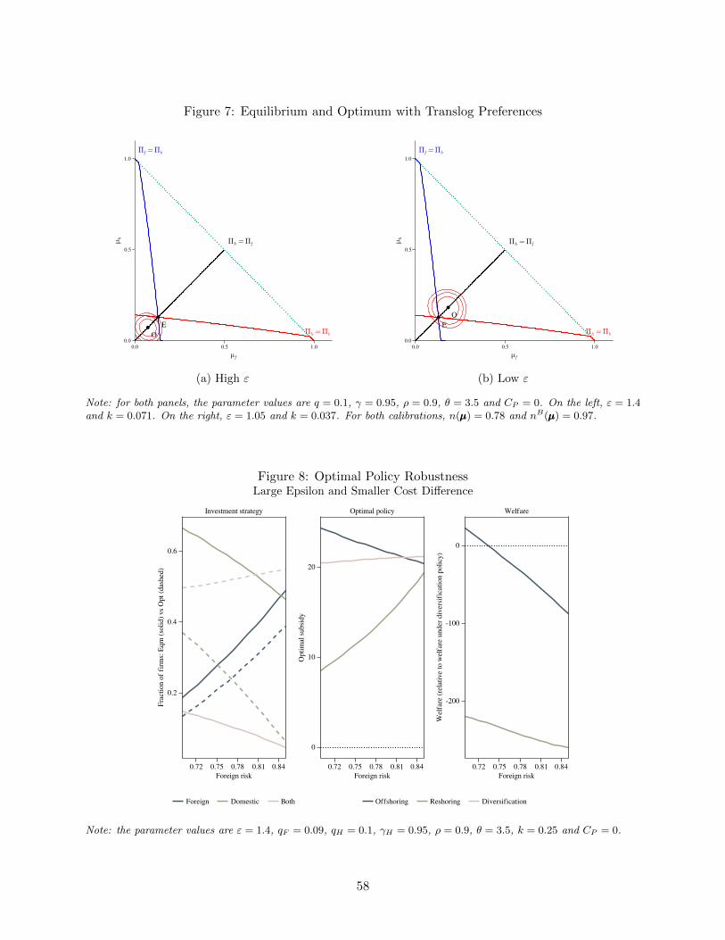
Figure 7: Equilibrium and Optimum with Translog Preferences

μf

0.0 0.5 1.0

μh

0.0

0.5

1.0

Πh = Πf

Πh = Πb

Πf = Πb

EO

(a) High ε

μf

0.0 0.5 1.0

μh

0.0

0.5

1.0

Πh = Πf

Πh = Πb

Πf = Πb

EO

(b) Low ε

Note: for both panels, the parameter values are q = 0.1, γ = 0.95, ρ = 0.9, θ = 3.5 and CP = 0. On the left, ε = 1.4and k = 0.071. On the right, ε = 1.05 and k = 0.037. For both calibrations, n(µµµ) = 0.78 and nB(µµµ) = 0.97.

Figure 8: Optimal Policy RobustnessLarge Epsilon and Smaller Cost Difference

Foreign risk0.72 0.75 0.78 0.81 0.84

Fra

ctio

n of

fir

ms:

Eqm

(so

lid)

vs O

pt (

dash

ed)

0.2

0.4

0.6

Investment strategy

Foreign risk0.72 0.75 0.78 0.81 0.84

Opt

imal

sub

sidy

0

10

20

Optimal policy

Foreign risk0.72 0.75 0.78 0.81 0.84

Wel

fare

(re

lati

ve to

wel

fare

und

er d

iver

sifi

cati

on p

olic

y)

-200

-100

0

Welfare

Foreign Domestic Both Offshoring Reshoring Diversification

Note: the parameter values are ε = 1.4, qF = 0.09, qH = 0.1, γH = 0.95, ρ = 0.9, θ = 3.5, k = 0.25 and CP = 0.

58

Figure 9: Optimal Policy RobustnessLarge Epsilon and Lower Idiosyncratic Risk

Foreign risk0.68 0.70 0.72 0.74

Fra

ctio

n of

fir

ms:

Eqm

(so

lid)

vs O

pt (

dash

ed)

0.0

0.1

0.2

0.3

0.4

0.5

0.6

Investment strategy

Foreign risk0.68 0.70 0.72 0.74

Opt

imal

sub

sidy

0

5

10

15

20

Optimal policy

Foreign risk0.68 0.70 0.72 0.74

Wel

fare

(re

lati

ve to

wel

fare

und

er d

iver

sifi

cati

on p

olic

y)

-400

-200

0

Welfare

Foreign Domestic Both Offshoring Reshoring Diversification

Note: the parameter values are ε = 1.4, qF = 0.08, qH = 0.1, γH = 0.95, ρ = 0.95, θ = 3.5, k = 0.25 and CP = 0.

Figure 10: Optimal Policy RobustnessSmall Epsilon and Larger Cost Difference

Foreign risk0.825 0.850 0.875

Fra

ctio

n of

fir

ms:

Eqm

(so

lid)

vs O

pt (

dash

ed)

0.2

0.4

0.6

Investment strategy

Foreign risk0.825 0.850 0.875

Opt

imal

sub

sidy

0

5

10

15Optimal policy

Foreign risk0.825 0.850 0.875

Wel

fare

(re

lati

ve to

wel

fare

und

er d

iver

sifi

cati

on p

olic

y)

-0.8

-0.6

-0.4

-0.2

0.0

Welfare

Foreign Domestic Both Offshoring Reshoring Diversification

Note: the parameter values are ε = 1.01, qF = 0.09, qH = 0.1, γH = 0.9, ρ = 0.9, θ = 3.5, k = 0.11 and CP = 0.

59

Figure 11: Optimal Policy RobustnessSmall Epsilon and Higher Idiosyncratic Risk

Foreign risk0.825 0.850 0.875

Fra

ctio

n of

fir

ms:

Eqm

(so

lid)

vs O

pt (

dash

ed)

0.1

0.2

0.3

0.4

Investment strategy

Foreign risk0.825 0.850 0.875

Opt

imal

sub

sidy

-5

0

5

Optimal policy

Foreign risk0.825 0.850 0.875

Wel

fare

(re

lati

ve to

wel

fare

und

er d

iver

sifi

cati

on p

olic

y)

0.00

0.05

0.10

Welfare

Foreign Domestic Both Offshoring Reshoring Diversification

Note: the parameter values are ε = 1.01, qF = 0.099, qH = 0.1, γH = 0.99, ρ = 0.95, θ = 3.5, k = 0.06 and CP = 0.

60