Supervised Dimensionality Reductionand Contextual Pattern Recognition

in Medical Image Processing

Marco Loog

this book was typeset by M. Loog using LATEX2ε� cover design by M. Loog

ISBN 90–393–3804–3

This work is subject to copyright. All rights are reserved, whether the whole or part of the material isconcerned, specifically the rights of translation, reprinting, reuse of illustrations, recitation, broadcasting,reproduction on microfilm or in any other form or by any other means, and storage in data banks, synapticweights, or hidden variables in electronic, mechanical, virtual or any other way. Permission for duplica-tion of this publication or parts thereof must always be obtained in writing from the author. Violationsare liable for prosecution.

Copyright c© 2004 Marco Loog

Printed by Ponsen & Looijen, Wageningen, The Netherlands

Supervised Dimensionality Reductionand Contextual Pattern Recognition

in Medical Image Processing

Gesuperviseerde dimensionaliteitsreductieen contextuele patroonherkenningin de medische beeldverwerking

(met een samenvatting in het Nederlands)

proefschrift

ter verkrijging van de graad van doctor aan de Universiteit Utrecht op gezagvan de Rector Magnificus, prof.dr. W. H. Gispen, ingevolge het besluit van hetCollege voor Promoties in het openbaar te verdedigen op dinsdag 14 september2004 des middags te 1245 uur

door

Marco Loog

geboren op 2 juni 1973 te Willemstad, Curacao

promotor Prof.dr.ir. M. A. ViergeverImage Sciences InstituteUniversity Medical Center Utrecht, The Netherlands

copromotoren Dr. B. van GinnekenImage Sciences InstituteUniversity Medical Center Utrecht, The Netherlands

Dr.ir. R. P. W. DuinFaculty of Electrical Engineering, Mathematics and Computer ScienceDelft University of Technology, The Netherlands

The research described in this thesis was carried out at the Image Sciences Institute, University MedicalCenter Utrecht, the Netherlands, under the auspices of ImagO, the Utrecht Graduate School for Biomed-ical Image Sciences. The project was financially supported by the Dutch Ministry of Economic Affairswithin the framework of the innovation-driven research program (IOP image processing, project numberIBV98002).

Financial support for publication of this thesis was kindly provided by Philips Medical Systems Neder-land B.V. (Medical IT - Advanced Development), the Rontgen Stichting Utrecht, and Utrecht University.

beoordelingscommissie Prof.dr. J. J. DuistermaatDepartment of MathematicsUtrecht University, The Netherlands

Prof.dr. R. D. GillDepartment of MathematicsUtrecht University, The Netherlands

Prof.dr.ir. B. M. ter Haar RomenyDepartment of Biomedical EngineeringEindhoven University of Technology, The Netherlands

Prof.dr. J. KittlerDepartment of Electronic and Electrical EngineeringUniversity of Surrey, United Kingdom

Prof.dr. M. ProkopDepartment of RadiologyUniversity Medical Center Utrecht, The Netherlands

de mani ere a obtenir un creuxErik Satie, Gnossienne No. 3

Contents

0 Introduction + Summary 10.1 On Features . . . . . . . . . . . . . . . . . . . . . . . . . . . . . . . . . . . . . . . . . . . . . . 20.2 On Classification . . . . . . . . . . . . . . . . . . . . . . . . . . . . . . . . . . . . . . . . . . . 40.3 On Image Processing for CAD in Chest Radiography . . . . . . . . . . . . . . . . . . . . . . 50.4 On Self-Containedness . . . . . . . . . . . . . . . . . . . . . . . . . . . . . . . . . . . . . . . . 6

1 A Heteroscedastic Extension of LDA:The Chernoff Criterion 71.1 The Chernoff Criterion: Two-Class Case . . . . . . . . . . . . . . . . . . . . . . . . . . . . . . 91.2 The Multi-Class Extension . . . . . . . . . . . . . . . . . . . . . . . . . . . . . . . . . . . . . . 121.3 Experimental Results . . . . . . . . . . . . . . . . . . . . . . . . . . . . . . . . . . . . . . . . . 141.4 Discussion + Conclusions . . . . . . . . . . . . . . . . . . . . . . . . . . . . . . . . . . . . . . 19

2 The Canonical Contextual Correlation Projection 212.1 Supervised Image Segmentation . . . . . . . . . . . . . . . . . . . . . . . . . . . . . . . . . . 232.2 LDA + a Direct Approach to Incorporating Context . . . . . . . . . . . . . . . . . . . . . . . 232.3 Canonical Contextual Correlation Projections . . . . . . . . . . . . . . . . . . . . . . . . . . . 252.4 An Illustrative Example . . . . . . . . . . . . . . . . . . . . . . . . . . . . . . . . . . . . . . . 292.5 Discussion + Conclusions . . . . . . . . . . . . . . . . . . . . . . . . . . . . . . . . . . . . . . 31

3 Nonparametric Local LinearDimensionality Reduction for Regression 353.1 Local Linear Dimensionality Reduction . . . . . . . . . . . . . . . . . . . . . . . . . . . . . . 363.2 Relative Influence of Predictors . . . . . . . . . . . . . . . . . . . . . . . . . . . . . . . . . . . 373.3 Concluding Remarks + Future Work . . . . . . . . . . . . . . . . . . . . . . . . . . . . . . . . 38

4 Iterated Contextual Pixel Classification 394.1 Iterated Contextual Pixel Classification . . . . . . . . . . . . . . . . . . . . . . . . . . . . . . . 414.2 Experimental Setup + Results . . . . . . . . . . . . . . . . . . . . . . . . . . . . . . . . . . . . 444.3 Discussion . . . . . . . . . . . . . . . . . . . . . . . . . . . . . . . . . . . . . . . . . . . . . . . 534.4 Conclusions . . . . . . . . . . . . . . . . . . . . . . . . . . . . . . . . . . . . . . . . . . . . . . 56

5 Segmentation of the Posterior Ribsin Chest Radiographsusing Iterated Contextual Pixel Classification 595.1 Materials . . . . . . . . . . . . . . . . . . . . . . . . . . . . . . . . . . . . . . . . . . . . . . . . 605.2 Iterated Contextual Pixel Classification . . . . . . . . . . . . . . . . . . . . . . . . . . . . . . . 615.3 Experiments, Results, + Evaluation . . . . . . . . . . . . . . . . . . . . . . . . . . . . . . . . . 695.4 Discussion + Conclusion . . . . . . . . . . . . . . . . . . . . . . . . . . . . . . . . . . . . . . . 73

6 Suppression of Bony Structuresfrom Projection Chest Radiographsby Dual Energy Faking 776.1 Materials + Methods . . . . . . . . . . . . . . . . . . . . . . . . . . . . . . . . . . . . . . . . . 796.2 Pilot + Leave-One-Out Experiments . . . . . . . . . . . . . . . . . . . . . . . . . . . . . . . . 816.3 Experimental Results . . . . . . . . . . . . . . . . . . . . . . . . . . . . . . . . . . . . . . . . . 836.4 Discussion + Conclusions . . . . . . . . . . . . . . . . . . . . . . . . . . . . . . . . . . . . . . 90

7 Notes 95

Bibliography 99

Een samenvatting in het Nederlands (A Summary in Dutch) 109

Acknowledgements 111

Published + Submitted Articles 113

Curriculum Vitae 117

0

Introduction + Summary

We write the year 2004 CE. The last few years have witnessed a significant increase in the number ofsupervised methods employed in diverse image processing tasks. Especially in medical image analysisthe use of, for example, supervised shape and appearance modelling [16, 18] has increased considerablyand has proven to be successful.

This thesis focuses on applying supervised pattern recognition methods [22, 28, 37, 47, 55, 90] in medi-cal image processing. We consider a local, pixel-based approach in which image segmentation, regression,and filtering tasks are solved using descriptors of the local image content (features) based on which de-cisions are made that provide a class label (in case of image segmentation) or a gray value (in case offiltering or regression) for every pixel. The basic probabilistic decision problem, underlying—implicitlyor explicitly—all the methods presented in this thesis, can be stated in terms of a conditional probabilityoptimization problem

ν = argmaxy∈Y

P(y|x) (1)

in which x ∈ Rd is a d-dimensional vector of measurements, i.e., a feature vector, describing the localimage content and y is an quantity that takes values from a set Y. Typically, in a classification task, Y is adiscrete set of labels and in case of regression, Y equals R. Based on the maximization in Equation (1), toevery vector x (which is associated to a pixel in an image), a particular ν from Y is associated.

This approach is—because of its local nature—quite different from the shape and appearance meth-ods mentioned in the beginning of this chapter which try to solve image processing tasks in a more globalway. A recent comparative study [42] shows that in image segmentation, pixel-based approaches cancompete with shape and appearance models, providing an interesting alternative to the latter.

The methodological part of the thesis consists of three dimensionality reduction methods (Chapters 1,2, and 3) that can aid the extraction of relevant features to be used for performing image segmentation orregression. Furthermore, in Chapter 4, an iterative segmentation scheme is developed which draws fromclassical pattern recognition and machine learning methods. Chapters 5 and 6 present the application ofthese techniques in two problems related to computer-aided diagnosis (CAD) in chest radiography. Chap-ter 5 considers the task of segmenting the posterior ribs while Chapter 6 presents a regression frameworkto suppress the bony structures in chest radiographs.

In the remainder of this introductory chapter, we provide an outline and summary of Chapters 1 to 6.

0.1 On Features

“Picking good features is the essence of pattern recognition,” as Ballard and Brown put it terse and in-sightful in their book on computer vision [3]. Indeed, it seems that there is not much more to it. Onceone or more good features have been selected1, solving the actual pattern recognition task is easy, if nottrivial. Clearly, the principal problem is to determine these good features.

In certain pixel-based image processing tasks, it is possible to design good features based on knowl-edge of the object to be segmented or detected. The object might be highly elongated or locally plate-likein which case features that detect such structures provide valuable information. Another possibility isthat the object of study has one or more distinctive gray values in which case the raw gray value in a pixelis an obvious feature to take into account. However, the more complicated the image processing problembecomes, the more intricate feature extraction will be and the more the usefulness of the features willdepend heavily on the insight and the talents of the person who tries to tackle the problem. Therefore,in many cases, one does not try to perform a thorough design of features for regression and classifica-tion purposes. Instead, many plausible features are extracted such that at least, hopefully, all relevantinformation is present in the feature vectors. Popular choices for features are outputs of Gaussian deriva-tive filters at several scales [34, 66, 73, 128], Gabor filters, raw pixel values in a certain neighborhood ofthe pixel under consideration, texture features, etc [10, 122, 88]. Although this approach often leads toreasonable results, it can suffer from substantial problems.

It is well known that, when adding more and more features in order to provide an object descriptionwhich is as accurate as possible, at a certain point, results start to deteriorate because the data becomeso high-dimensional that eventually it is impossible to obtain accurate estimates of parameters or anyother quantity2. This phenomenon bares the daunting name the curse of dimensionality—a term coinedby Bellman [5], and can be encountered in several other guises, e.g. as overfitting in regression (see also[120]).

Supervised dimensionality reduction methods provide heuristics to overcome—or rather, try to dealwith—this curse. They aim at determining an appropriate subspace in the original feature space in whichall relevant information, that was initially present in the high-dimensional feature space, is still avail-able. (A well-known unsupervised dimensionality reduction technique is principal component analysis(PCA), which is also known as the Karhunen-Loeve expansion [89].) Subsequently, complex classifica-tion and regression schemes can be built more accurately in this lower-dimensional space and, as such,an improvement in performance is well possible. Clearly, such approaches have a potential applicationin feature design. Collecting a large amount of image features followed by an appropriate dimension-ality reduction can provide an effective and relatively compact local image description that can be usedin supervised image processing tasks, thus offering a data-driven and task dependent approach to thisproblem.

1In case of a classification task, preferably those features should be selected that take on values equal to the classnumber to which the objects should be classified.

2As an example, consider estimating a full covariance matrix in a d-dimensional space using N feature vectors, whereN < d.

2

In Chapter 1, an eigenvector-based heteroscedastic3 linear dimension reduction (LDR) technique formulti-class data is presented. The technique is based on a heteroscedastic two-class technique which uti-lizes the so called Chernoff criterion, and successfully extends the well-known linear discriminant analy-sis (LDA). The latter, which is based on the Fisher criterion, is incapable of dealing with heteroscedasticdata in a proper way.

For the two-class case, the between-class scatter is generalized so as to capture differences in(co)variances. It is shown that the classical notion of between-class scatter can be associated with Eu-clidean distances between class means. From this viewpoint, the between-class scatter is generalizedby employing the Chernoff distance measure, leading to our proposed heteroscedastic measure. Finally,using the results from the two-class case, a multi-class extension of the Chernoff criterion is proposed.This criterion combines separation information present in the class mean as well as the class covariancematrices.

The approach is of particular interest in classification tasks dealing with only few classes because itovercomes the severe restriction of LDA being able to only reduce the dimensionality of the feature spaceto a maximum of K − 1 dimensions, where K is the number of classes. In image processing K is often 2,e.g. the object and the background class and chances are small that all relevant information is captured inthe single feature obtained by LDA.

Extensive experiments and a comparison with similar dimension reduction techniques demonstratethe potential of the Chernoff-based technique, which is also used in Chapter 5.

While Chapter 1 provides a reduction technique that is generally applicable in a supervised classifica-tion framework, Chapter 2 presents a technique that aims at exploiting contextual information as presentin, for example, image data and the like. The technique is called the canonical contextual correlationprojection (CCCP).

Again, the method is derived from classical linear discriminant analysis (LDA), extending this tech-nique to cases where there are dependencies between the output variables, i.e., the class labels, and notonly between the input variables. (The latter can readily be dealt with in standard LDA.) The novelmethod is useful, for example, in supervised segmentation tasks in which high-dimensional feature vec-tors describe the local structure of an image.

The principal idea is that where standard LDA merely takes into account a single class label for everyfeature vector, CCCP incorporates class labels of its neighborhood in the analysis as well. In this way,the spatial class label configuration in the vicinity of every feature vector is accounted for, resulting in atechnique suitable for e.g. image data.

As noted earlier, an additional drawback of LDA is that it cannot extract more features than thenumber of classes minus one. In the two-class case this means that only a reduction to one dimensionis possible. Like the technique proposed in Chapter 1, our contextual approach can avoid such extremedeterioration of the classification space and retain more than one dimension.

3Heteroscedasticity of the data means, in this case, that the covariance matrices of the different classes present in thedata are not equal.

3

CCCP is exemplified on a pixel-based medical image segmentation problem in which it is shown thatit can give significant improvement in segmentation accuracy.

A third reduction technique is described in Chapter 3. As opposed to the former two, which deal withclassification tasks, this technique can be used to linearly reduce the dimensionality of predictor variablesin a multivariate regression setting. The method specifically aims for the improvement of regressionresults when employing nonparametric techniques.

Two straightforward ways of performing linear dimensionality reduction for regression are perform-ing a principal component analysis (PCA) on the predictor variables, or performing a linear regression onthe data and use the regressed data as the new predictor. The drawback of the former approach is that itis completely unsupervised as it does not take the response variables into account. The latter approachsuffers from the fact that it can only retain a single predictor variable, which will in most cases not sufficeto make an accurate prediction.

The class of heuristics proposed in this chapter builds on the latter linear regression-based approach.However, instead of solving it globally, a local approach based on a k-nearest neighbor technique is con-sidered by which estimates of local linear dimensionality reductions are determined. These local esti-mates are subsequently combined, via a PCA, from which a global linear dimension reduction can bedetermined.

An example of the possible improvements to which employing this technique can lead is given inChapter 6.

0.2 On Classification

In Chapters 1 to 3, we introduced three different dimensionality reduction techniques that facilitate andimprove the feature extraction stage in supervised pattern recognition and machine learning schemes.Such schemes can be readily employed to perform image segmentation (via pixel classification) or imageregression (through pixel-based regression), and frequently can attain reasonable, or even good, perfor-mance. Nonetheless, image segmentations obtained by means of pixel classification seem amenable toimprovements. Many a time, the borders of the segments are granular and not smooth and well-defined.Moreover, single pixels, or slightly larger structures, are often misclassified and show up as a pattern ofspeckles and spots in the segments.

In many of the previous cases it is obvious from the contextual class label information which pixels arelabelled erroneous and how they should be relabelled to improve the segmentation. Chapter 4 presents ageneral data-driven image segmentation scheme that iteratively tries to correct mislabelled pixels by tak-ing contextual class label information into account. The scheme utilizes supervised classification methodsand easily incorporates other common techniques from pattern recognition and machine learning.

The method, called iterated contextual pixel classification (ICPC), is in principle pixel-based and doesnot take an explicit global or geometric model into account. However, ICPC does exploit local contextualclass label information that is present in the data and employs this information to come to a good overallsegmentation.

4

ICPC can be considered a supervised variant of Besag’s iterated conditional modes (ICM, [7, 8]):Starting from an initial segmentation, the algorithm iteratively updates it by reclassifying every pixel,based on the features used for the initial classification (e.g. gray level features) and, in addition, localstructural information from the spatial context. This latter contextual information typically consists of theclass labels of pixels in the vicinity of the pixel to be reclassified.

To illustrate the capabilities of the technique, in this chapter, some specific instances of the methodare compared to each other and to (non-iterative) pixel classification. This is done experimentally on twomedical image segmentation tasks. The first one is the segmentation of vessels in fundus photographs andthe second is the delineation of the lung fields in chest radiographs. Subsequently, Chapter 5 presentsan application of ICPC in the delineation of posterior ribs in chest radiographs. In this latter chapter,dimensionality reduction approaches also proofs to be valuable in dealing with the high-dimensionalcontextual class label information.

0.3 On Image Processing for CAD in Chest Radiography

The final two chapters of this thesis, Chapters 5 and 6, give two worked-through examples of how pat-tern recognition and machine learning techniques can be used to perform image processing and analysistasks. Both tasks presented are possible steps in a computer-aided diagnosis (CAD) system dealing withposteroanterior chest radiographs and mainly focusing on the detection of lung nodules (see, for example,[111]). In addition, the technique may also proof to be valuable in systems detecting interstitial diseaselike for example tuberculosis (see, for example, [41, 82], cf. [83]).

In Chapter 5, the task of segmenting the posterior ribs within the lung fields of standard posteroante-rior chest radiographs is considered. Precise identification of the ribs can aid in the detection of rib lesionsand the localization of lung lesions.

To perform the segmentation, ICPC is used. The method is evaluated on 30 radiographs taken fromthe JSRT (Japanese Society of Radiological Technology) database. All posterior ribs within the lung fieldsin these images have been traced manually by two observers. The first observer’s segmentations are setas the gold standard; ICPC is trained using these segmentations. In a six-fold cross validation experimentICPC achieves a classification accuracy of 0.86 ± 0.06, as compared to 0.94 ± 0.02 for the second humanobserver.

Instead of segmenting the ribs, another possibility to improve the performance of a CAD systemfor chest radiographs is by introducing a stage that tries to remove or suppress irrelevant anatomicalstructures from the image. Examples of irrelevant structures in posteroanterior chest radiographs arebony structures. Removing these kinds of structures can be done quite effectively if the right dual energyimages—two radiographic images from the same patient taken with different energies—are available.Subtracting these two radiographs gives a soft-tissue image with most of the rib and other bony structuresremoved. In general, however, dual energy images are not readily available.

Chapter 6 proposes a supervised learning technique for inferring a soft-tissue image from a standardradiograph without explicitly determining the additional dual energy image. The procedure, called dual

5

energy faking, is based on k-nearest neighbor regression, and incorporates knowledge obtained from atraining set of dual energy radiographs with their corresponding subtraction images for the constructionof a soft-tissue image from a previously unseen single standard chest image.

0.4 On Self-Containedness

This thesis is not self-contained and the reader may want to consult one or two textbooks on patternrecognition—being the main topic of this thesis—and related fields. We suggest one or more of the earliermentioned general works: [22], [28], [37], [47], [55], and [90]. In addition, we refer the reader to [123] or[23] for a more mathematical approach to machine learning and pattern recognition.

6

1

A Heteroscedastic Extension of LDA:The Chernoff Criterion

Linearly reducing the dimensionality of the features space, i.e. feature extraction, is a common techniquein statistical pattern recognition typically used to lower the size of statistical models and overcome estima-tion problems, often resulting in an improved classifier accuracy in this lower-dimensional space. Lineardiscriminant analysis (LDA) is probably the most well-known approach to supervised linear dimension re-duction (LDR). This classical technique was developed by Fisher [32] for the two-class case, and extendedby Rao [100] to handle the multi-class case.

In LDA, a transformation matrix from an n-dimensional feature space to a d-dimensional space isdetermined such that the Fisher criterion of between-class scatter over within-class scatter is maximized(cf. [22, 37, 55, 90]). An attractive feature of LDA is the fast and easy way to determine this optimallinear transformation, only requiring simple matrix arithmetics. A limitation of LDA is that it merelytries to separate class means as good as possible, and it does not take the discriminatory information thatis present in the difference of the covariance matrices into account. It is incapable of dealing explicitlywith heteroscedastic data, i.e., data in which classes do not have equal covariance matrices. This limitationbecomes very apparent in the two-class case, in which a reduction to only a single dimension is possible(cf. [37]), while the K-class case allows only for a reduction to at most K − 1 dimensions.

When linearly reducing the dimensionality, the K − 1 dimensions do not necessarily contain all therelevant data for the classification task, and even if K − 1 dimensions do so, it is not clear that LDA willdiscern them. Taking the heteroscedasticity of the data into account, we develop an LDR technique thatextends and improves upon classical LDA. This extension is obtained via the use of directed distancematrices (DDMs) [77], which can be considered generalizations of the between-class scatter matrix. Thebetween-class scatter matrix, as used in LDA, merely takes into account the discriminatory informationthat is present in the pairwise differences of class means, and can be associated with the squared Euclideandistance between pairs of class means.

The specific heteroscedastic extension of the Fisher criterion, studied more closely in Sections 1.1and 1.2, is based on the Chernoff distance [13, 14]. This measure of affinity of two densities considers meandifferences as well as covariance differences—as opposed to the Euclidean distance—and is used to extendLDA. Section 1.1 discusses the LDA extension for two-class data as proposed in an earlier article [78]. InSection 1.2, we come to our heteroscedastic multi-class measure, which extends LDA, by comparing the

K classes in a pairwise fashion and using the two-class measure as a building block. While doing so, weretain the attractive feature of fast and easily determining a dimension reducing transformation, as withLDA. Furthermore, we are able to reduce the data to any dimension d smaller than n and not only to, atmost, K − 1 dimensions.

In Section 4.2 of [37], Fukunaga discusses several ways of extending the linear classifiers to unequalcovariance matrices and non-normal distributions. The criteria derived can also be used for the purposeof dimensionality reduction. However, besides the fact that they are merely derived for the two-class caseand not readily extendible to the multi-class case, the criteria essentially give a single LDR vector thattakes the difference between the class means into account. In addition some of the approaches need aniterative optimization procedure.

Several alternative approaches to heteroscedastic LDR (HLDR) are known, of which we mention thefollowing ones. See also [22], [37], and [90], and references therein.

Under the assumption that all classes are normally distributed, [105] gives a computationally de-manding approach to solving the LDR problem by minimizing the actual Bayes error in the linearly re-duced space. This is done using simulated annealing in combination with an exact integration over thelower-dimensional feature space.

Straightforward extensions of the Fisher criterion were proposed in [21] and [93], the former of whichis based on the Kullback divergence. As opposed to our criterion, their iterative optimization proceduresare clearly more complex than optimizing the Fisher criterion. A broad overview of feature extractiontechniques based on probabilistic separability and interclass distance measures—some of them relatedto the previous mentioned techniques—can be found in [22]. Again, mostly, time-consuming iterativeprocedures should be employed to optimize these criteria.

Different extensions of Fisher’s LDA are given by Hastie et al., see [47]. We mention penalized dis-criminant analysis (PDA), which can also be used for the purpose of LDR. By means of regularizationPDA is able to deal with data in which one has many highly correlated features and LDA would sufferfrom overfitting. However, PDA does not explicitly use the discriminatory information present in thecovariance terms as the Chernoff criterion does. We note that the regularizations suggested for PDA arereadily applicable within our approach.

Another multi-class HLDR procedure, which is based on a maximum likelihood formulation of LDA,is studied in [67]. Here LDA is generalized by dropping the assumption that all classes have equal within-class covariance matrices, and iteratively maximizing the likelihood for this model.

Of the computationally intensive methods, we finally mention the nonparametric approaches pre-sented in [12] and [75]. These techniques work directly on the data and try to maintain as much of theseparation information as possible in the lower-dimensional space. The amount of separability in thesubspace is measured using a certain nearest neighbor procedure, which accounts for a large part of thecomputational complexity. Comparable to these approaches is the one given in [22] based on Parzenestimates.

Two fast LDR methods based on the singular value decomposition (svd) were introduced in [121] and[11], respectively. The first one by Tubbs et al. presents an HLDR method while the latter is Mahalanobis

8

distance-based and basically homoscedastic. We describe both methods in some more details in Section1.3, where we also compare our non-iterative method to theirs and to LDA on twelve real-world data setsfrom the UCI Repository [92].

Section 1.4 completes the chapter with a discussion and the conclusions.

1.1 The Chernoff Criterion: Two-Class Case

The Fisher criterion

LDR is concerned with the search for a linear transformation that reduces the dimension of a given n-dimensional statistical model to d (d < n) dimensions, while maximally preserving the discriminatoryinformation for the several classes within the model. Due to the complexity of utilizing the Bayes erroras the criterion to optimize, one resorts to suboptimal criteria. LDA is such a suboptimal approach. Itdetermines a linear mapping L, a d × n-matrix, that maximizes the so-called Fisher criterion JF [37, 55, 77,100]:

JF(A) = tr((ASW At)−1(ASBAt)) . (1.1)

Here SB := ∑Ki=1 pi(mi − m)(mi − m)t and SW := ∑K

i=1 piSi are the between-class and the average within-class scatter matrix, respectively; K is the number of classes, mi is the mean vector of class i, pi is its apriori probability, and the estimated overall mean m equals ∑K

i=1 pimi . Furthermore, Si is the within-classcovariance matrix of class i, and A is a d × n-matrix. From Equation (1.1) we see that LDA maximizes theratio of between-class scatter to average within-class scatter in the lower-dimensional space. Optimizing(1.1) comes down to determining an eigenvalue decomposition of S−1

W SB, and taking the rows of L toequal the d eigenvectors corresponding to the d largest eigenvalues [22, 37].

This section focusses on the two-class case, in which case we have SB = p1 p2(m1 − m2)(m1 − m2)t

[37, 77, 78], SW = p1S1 + p2S2, and p1 = 1 − p2. Note that in this case the rank of SB is 1—assumingunequal class means, and so we can only reduce the dimension to 1. According to the Fisher criterionthere is no discriminatory information in the features, apart from this single dimension.

Directed distance matrices

For now, assume that the data is linearly transformed such that the within-class covariance matrix SWequals the identity matrix, then JF(A) equals tr((AAt)−1(Ap1 p2 (m1 − m2)(m1 − m2)tAt)), which ismaximized by taking the eigenvector v associated with the largest eigenvalue λ of the matrix SE := (m1 −m2)(m1 − m2)t. (Note that SB = p1 p2 SE) This matrix has only one nonzero eigenvalue, which equalsλ = tr((m1 −m2)(m1 −m2)t) = (m1 −m2)t(m1 −m2), with associated eigenvector v = m1 −m2. Notethat the eigenvalue equals the squared Euclidean distance, denoted by ∂E, between the two class means.

The matrix SE := (m1 − m2)(m1 − m2)t not only gives us the distance between two distributions,but it also provides the direction, by means of the eigenvectors, in which this specific distance can befound. As a matter of a fact, if both classes are normally distributed and have equal covariance matrices,there is only distance between them in the direction v and this distance equals λ. All other eigenvectors

9

have eigenvalue 0, indicating that there is no distance between the two classes in these directions. Indeed,reducing the dimension using one of these latter eigenvectors results in a complete overlap of the classes:There is no discriminatory information in these directions, the distance equals 0.

The idea behind directed distance matrices (DDMs) is to give a generalization of SE and hence SB[77]. If there is discriminatory information present because of the heteroscedasticity of the data, thenthis should become apparent in the DDM. This extra distance due to the heteroscedasticity, is, in general,in different directions than the vector v, which separates the means, and so DDMs have more than onenonzero eigenvalue.

The specific DDM we propose is based on the Chernoff distance ∂C between two probability densityfunctions d1 and d2

∂C := − log∫

dα1 (x) d1−α

2 (x)dx ,

where α ∈ (0, 1) is a constant1.

For two normally distributed densities, it equals2 [13, 14]

∂C =(m1 −m2)t(αS1 + (1 −α)S2)−1(m1 −m2)

+1

α(1 −α)log

|(αS1 + (1 −α)S2)||S1|α |S2|1−α

.(1.2)

Like ∂E, we can obtain ∂C as the trace of a positive semi-definite matrix SC (cf. [77]):

SC :=S−12 (m1 −m2)(m1 −m2)tS−

12

+1

α(1 −α)(log S −α log S1 − (1 −α) log S2) ,

(1.3)

where S := αS1 + (1 −α)S2, S−12 is the inverted square root and log S is the logarithm3 of S.

1N.B. in [19], the Chernoff distance is defined as the minimum of ∂C over all α ∈ (0, 1).2Although the Chernoff distance actually equals α(1−α)

2 ∂C in this case, this constant factor is of no essential influenceon the rest of our discussion.

3We define the function f , e.g. some power or the logarithm, of a symmetric positive definite matrix A, bymeans of its eigenvalue decomposition RVR−1 , with eigenvalue matrix V = diag(v1 , . . . , vn). We let f (A) equalR diag( f (v1), . . . , f (vn)) R−1 = R( f (V))R−1 . Although generally A is nonsingular, determining f (A) might cause nu-merical problems, if the matrix is close to singular. Alleviation of this computational problem is possible by using thesvd instead of an eigenvalue decomposition, or by properly regularizing A.

10

To see that the trace of SC equals ∂C , write out tr SC :

tr SC =tr(S−12 (m1 −m2)(m1 −m2)tS−

12 )

+tr(

1α(1 −α)

(log S −α log S1 − (1 −α) log S2))

=tr((m1 −m2)tS−1(m1 −m2))

+1

α(1 −α)(tr(log S)−α tr(log S1)

− (1 −α) tr(log S2))

=(m1 −m2)tS−1(m1 −m2)

+1

α(1 −α)(log |S| −α log |S1| − (1 −α) log |S2|) .

Finally, recalling that S := αS1 + (1 −α)S2 and combining the three logarithms into a single one, we seethat the resulting expression equals (1.2).

We want the final criterion to be an extension of Fisher’s, so if the data is homoscedastic, i.e., S1 = S2,we want SC to equal SE. This suggests to set α equal to p1, from which it directly follows that 1−α equalsp2. The link with homoscedastic LDA is clear from the foregoing.

To exemplify the behavior of the matrix SC in the heteroscedastic case we consider the other extremecase in which the means are taken to be equal, i.e., m1 = m2. In addition, assume that S1 and S2 arediagonal, diag(a1 , . . . , an) and diag(b1 , . . . , bn), respectively, but not necessarily equal. Because α = p1,and αS1 + (1 −α)S2 = I (by assumption), we have

SC =1

p1 p2diag(log

1ap1

1 bp21

, . . . , log1

ap1n bp2

n) . (1.4)

On the diagonal of SC are the Chernoff distances of the two densities if the dimension is reduced to onein the associated direction, e.g., linearly transforming the data by the n-vector (0, . . . , 0, 1, 0, . . . , 0), whereonly the dth entry is 1 and all the others equal 0, would give us a Chernoff distance of 1

p1 p2log 1

ap1d b

p2d

in

the one-dimensional space. Hence, determining a LDR transformation by an eigenvalue decompositionof the DDM SC , means that we determine a transform which preserves as much of the Chernoff distancein the lower dimensional space as possible.

In view of the two cases above, we argue that our suggested DDM gives eligible results. In addition,we argue that this even holds if we do not have equality of means or covariance matrices, because alsoin this case we obtain a solution that is based on the Chernoff distance, which is a certain weightedcombination of both extreme cases above. In conclusion: The DDM SC , captures differences in covariancematrices and indeed gives an extension of the homoscedastic DDM SE.

11

The two-class Chernoff criterion

If SW = I, JF(A) equals tr((AAt)−1(p1 p2 ASEAt)). Therefore, in this case, regarding the discussion inthe foregoing subsection, we simply substitute SC for SE, to obtain a heteroscedastic generalization of

the Fisher criterion. In case SW 6= I, we first transform the data by S− 1

2W , so we do have SW = I. In this

space, the criterion is determined—which for LDA equals tr((AAt)−1(p1 p2 AS− 1

2W SES

− 12

W At)), and then

transformed back to the original space using S12W . For the Fisher criterion this would finally result in

tr((AS12W S

12W At)−1(p1 p2 ASEAt)) ,

which equals (1.1), as if it was determined directly in the original space. Using SC instead of SE,thisprocedure leads to the following heteroscedastic extension.Definition. The heteroscedastic two-class Chernoff criterion JC is defined as

JC(A) := tr((ASW At)−1(p1 p2 A(m1 −m2)(m1 −m2)tAt

−AS12W(p1 log(S

− 12

W S1S− 1

2W ) + p2 log(S

− 12

W S2S− 1

2W ))S

12W At)) .

(1.5)

1.2 The Multi-Class Extension

In the previous section, we derived the Chernoff criterion for two-class data (see also [78]). In this sectionwe turn to the multi-class case. Based on a certain decomposition of the between-class scatter matrix, weconstruct a measure for HLDR using the two-class criterion as a building block.

Decomposing the between-class scatter matrix

The decomposition of the between-class scatter matrix SB we use to generalize the Chernoff criterion tothe multi-class case is as follows

SB =K−1

∑i=1

K

∑j=i+1

pi p j(mi −m j)(mi −m j)t

=K−1

∑i=1

K

∑j=i+1

pi p j SEi j ,

(1.6)

where SEi j := (mi −m j)(mi −m j)t. (See [77] for a proof of Equivalence (1.6) above.) This decompositionshows how the scatter matrix captures the divergence of the class mean mi from all other class means m j.For every pair of means the difference vector mi − m j is determined and the sum of their outer productsforms the between-class scatter.

12

Based on Equality 1.6, JF can be decomposed as

JF(A) =K−1

∑i=1

K

∑j=i+1

pi p j tr((ASW At)−1(ASEi jAt)) . (1.7)

Foregoing expression allows a decomposition of the Fisher criterion into a sum of pairwise Fisher crite-ria. It consists of sums of Fisher criteria taken all class pairs into account separately (cf. [77]). Based onthis pairwise decomposed Fisher criterion, we can now generalize the two-class Chernoff criterion to themulti-class case.

Weighted two-class Chernoff criteria: The heteroscedasticization of Fisher

Initially, as in Section 1.1, the within-class scatter SW is assumed to equal the identity matrix. In this casethe Fisher criterion equals tr((AAt)−1(ASBAt)), which can be optimized via an eigenvalue decomposi-tion of the matrix SB. Decomposition (1.6) shows that SB is a weighted sum of pairwise DDMs, and assuch can be considered a DDM itself: Its eigenvectors giving the direction in which there is distance, theireigenvalues giving the actual distance. Indeed, carrying out an LDA and assuming the within-class scat-ter matrix to be the identity, LDR is performed by taking those eigenvectors of SB for which the associatedeigenvalues are largest.

In light of Subsections 1.1 and 1.1, and Decomposition (1.7), foregoing considerations lead us to theChernoff-based, multi-class extension of the two-class Chernoff criterion.

JC(A) :=K−1

∑i=1

K

∑j=i+1

pi p j tr((AAt)−1(ASCi jAt)) . (1.8)

In this, SCi j is the DDM capturing the Chernoff distance between class i and j, which is immediatelydetermined by means of Equation (1.3).

SCi j :=S− 1

2i j (mi −m j)(mi −m j)tS

− 12

i j

+1

πi π j(log Si j − πi log Si − π j log S j) .

(1.9)

Here πi := pi/(pi + p j), and π j := p j/(pi + p j) are relative priors, i.e., only taking the two classes intoaccount that define the particular pairwise term. Furthermore, Si j is the average pairwise within-classscatter matrix, defined as πi Si + π j S j.

Along the same line of reasoning as in Subsection 1.1, the final multi-class Chernoff criterion—inwhich the within-class scatter is not necessarily the identity matrix—can be obtained by first transformingthe data such that the within-class scatter matrix is the identity, then determine the criterion JC, and finallydo the inverse transformation, leading to

13

Definition. For a d × n-matrix A, the multi-class measure of spread JC, the Chernoff criterion, is defined as

JC(A) :=K−1

∑i=1

K

∑j=i+1

pi p j tr((ASW At)−1

×AS12W

((S

− 12

W Si jS− 1

2W )−

12 S

− 12

W (mi −m j)(mi −m j)tS− 1

2W (S

− 12

W Si jS− 1

2W )−

12

+1

πi π j((log S

− 12

W Si jS− 1

2W )− πi log(S

− 12

W SiS− 1

2W )− π j log(S

− 12

W S jS− 1

2W ))

)S

12W At

),

(1.10)

where πi := pi/(pi + p j), π j := p j/(pi + p j), and Si j := πi Si + π j S j.The Chernoff criterion is maximized in a manner similar to optimizing the Fisher criterion: First

determine an eigenvalue decomposition of the n × n-matrix

K−1

∑i=1

K

∑j=i+1

pi p j S−1W × S

12W

((S

− 12

W S− 1

2i j S

− 12

W )S− 1

2W (mi −m j)(mi −m j)tS

− 12

W (S− 1

2W Si jS

− 12

W )−12

+1

πi π j(log(S

− 12

W Si jS− 1

2W )− πi log(S

− 12

W SiS− 1

2W )− π j log(S

− 12

W S jS− 1

2W ))

)S

12W ,

(1.11)

then take the rows of the transformation matrix L to equal the d eigenvectors associated with the d largesteigenvalues [22, 37].

Note that in the two-class case S− 1

2W Si jS

− 12

W = I, hence the foregoing weighted two-class Chernoffcriterion boils down to the original two-class Chernoff criterion (1.5). Note also that if all covariancematrices Si are equal, the Chernoff criterion equals the Fisher criterion, i.e., JC = JF.

1.3 Experimental Results

This section compares the performance of the HLDR transformations obtained by means of the Chernoffcriterion—based on an eigendecomposition of the matrix in (1.11)—with transformations obtained by thetraditional Fisher criterion. In addition, the performances of the HLDR methods from [121] and [11], arealso compared to the performance of the Chernoff criterion. For some other comparative studies, betweenseveral LDR techniques on several data sets, see for example [1] and [11].

The method in [121] determines a heteroscedastic dimension reducing transform by constructing ann × (n + 1)(K − 1)-matrix T that equals (m2 − m1 , . . . , mK − m1 , S2 − S1 , . . . , SK − S1), then performingan svd on T = QSVt, and finally choosing the column vectors from Q associated with the largest dsingular values as the LDR transformation. As with our HLDR approach, this approach also allows forLDR to dimensions larger than K − 1 (if K − 1 < n) and up to n.

Similar to the foregoing method is the Mahalanobis distance-based method from [11], which de-termines an svd QSVt of the n × 1

2 n(n − 1)-matrix U = ((S1 + S2)−1(m1 − m2), (S1 + S3)−1(m1 −m3), . . . , (SK−1 + SK)−1(mK−1 − mK)). Again, the column vectors from Q associated with the largest dsingular values are chosen as the LDR transformation. This technique can also be viewed as an extension

14

Table 1.1 . The 12 data sets taken from [92] used in the experiments. Information is provided on initial di-mensionality n, dimensionality after principal component analysis PC, number of classes K, and numberof total instances N.

data set label n PC K NWisconsin breast cancer (a) 9 9 2 682BUPA liver disorder (b) 6 6 2 345Pima indians diabetes (c) 8 8 2 768Wisconsin diagnostic breast cancer (d) 30 7 2 569Cleveland heart-disease (e) 13 13 2 297SPECTF heart (f) 44 44 2 349Iris plants (g) 4 4 3 150Thyroid gland (h) 5 5 3 215Vowel context (i) 10 10 11 990Landsat satellite (j) 36 36 6 6435Multi-feature digit (Zernike moments) (k) 47 33 10 2000Glass identification (l) 9 8 6 214

to Fisher’s LDA and allows for a reduction of dimensionality up to d = 12 K(K − 1) (if 1

2 K(K − 1) ≤ n, see[11]).

Tests were performed on twelve real-world data sets, labelled (a) to (l), taken from the UCI Repositoryof machine learning databases [92] (see Table 1.1). Instances with missing values were taken out of thedata sets prior to the experiments.

The comparison is based on two different classifiers [22, 37, 55]:

� The linear classifier assuming all classes to be normally distributed with equal covariance matrix.

� The quadratic classifier assuming the underlying distributions to be normal with covariance ma-trices that are not necessarily equal.

These two classifiers are chosen, because they stay close to the assumption that most of the relevantinformation is in the first and second order central moments, i.e., the means and the (co)variances. Thefirst classifier merely takes means and average within-class covariances into account based upon whichlinear decision boundaries are constructed. The second can cope with all classes having different meansand covariance matrices and allows the decision boundaries to be quadratic.

The experimental setup

For every of the twelve data sets and for every possible d to reduce the dimension to, the experimentdescribed below is conducted a hundred times.

15

1. The data set is randomly split into a test and a train set. The test set contains (approximately) 10%of the data, while the train set contains the remaining 90%.

2. A PCA is performed on the train set after which all principal components with an eigenvaluesmaller than one millionth of the total variance, i.e., the trace of the total covariance matrix, arediscarded. In this way, problems related to (near) singular covariance matrices are avoided andall four transformations can be properly determined. See Table 1.1 for the data dimensionalitiesbefore and after PCA. Note that for most data sets all principal components are retained.

3. Using the transformed train data, we determine the four LDR transformations (or less, if a reduc-tion to d dimensions is not possible with a certain transformation, i.e., the Fisher-based and theMahalanobis distance-based transformations) and reduce the dimensionality of the train data to d.

4. In the d-dimensional reduced feature space we determine the linear and the quadratic classifierusing the train data, and subsequently classify the test data after transforming its instances in thesame way as the train instances. The classification error is estimated on the test data.

Analysis of results

The per data set-performances of the several LDR techniques are compared. To this end, per classifier, dataset and dimension d, the mean estimated classification error over the hundred runs is determined. Thisgives a final estimate of the classification error for the respective settings. For every LDR transform, onlythe optimal dimensionality to reduce the data to and the corresponding mean classification error (MCE)is reported. (Our method, as well as the other methods give no direct means to determine an optimaldimensionality to reduce to. However, the observed optimal MCEs give an indication of the attainableperformance and can be used to compare the several approaches.) These numbers are presented in Table1.2 and Table 1.3. The overall optimal MCE over all transforms is typeset in bold and a ‘∗’ is addedin superscript. Also in bold are the transforms that give, in comparison to the optimal transformation,statistically indiscernible classification errors. For this, results are compared using a signed rank test inwhich the desired level of significance is set to 0.01 (see [102]). If it is possible to attain an MCE notsignificantly different—again based on a signed rank test—from the optimal one in a lower-dimensionalspace, this is indicated by the second integer in parentheses on the right of the /. Tables 1.2 and 1.3 alsogive the MCE obtained when not performing an LDR.

We start with two general observations. First, the quadratic classifier performs in general better formost data sets. The two exceptions are data sets (g) and (l). This may indicate that in most data setsthere is indeed separation information present in the second order moments of the class distributions.Second, we see that LDR indeed can improve the accuracy of the classifier in most cases. Note, although,that this is not always the case (take for example data set (i) and the quadratic classifier) and if it doeshold the improvements are sometimes not very convincing. However, even if the error rate does notdrop considerably, the feature dimensionality often does, and we can attain similar error rates in featurespaces having much lower dimensionality than the initial space. Very often even a reduction to a singledimension is possible.

16

Table 1.2 . Observed MCE and optimal dimensionality (d) for the twelve data sets (a) to (l), using thelinear classifier and the four different LDR techniques indicated by ‘Fisher’, ‘Chernoff’, ‘Tubbs’ [121], and‘Mahalanobis’ [11]. Optimal observed MCE per data set is typeset in bold and a superscript ∗ is added.Also in bold are the MCEs for transforms that give, in comparison to the optimal transformation, indis-cernible MCEs based on a signed rank test with significance level 0.01. An MCE in a lower-dimensionalspace indiscernible from the optimal one, is indicated by the second integer in parentheses on the right ofthe /. The estimated MCE using no LDR is below ‘Full’.

Full Fisher Chernoff Mahalanobis Tubbslabel MCE MCE (d) MCE (d) MCE (d) MCE (d)(a) 0.063 0.047 (1) 0.046∗ (1) 0.047 (1) 0.050 (2)(b) 0.426 0.427 (1) 0.424∗ (1) 0.427 (1) 0.428 (5)(c) 0.348 0.348∗ (1) 0.348∗ (2/1) 0.349 (1) 0.348∗ (5/4)(d) 0.142 0.177 (1) 0.131∗ (1) 0.208 (1) 0.140 (3)(e) 0.175 0.172 (1) 0.171∗ (1) 0.175 (1) 0.174 (12/5)(f) 0.279 0.272 (1) 0.266 (2) 0.239 (1) 0.205∗ (6)(g) 0.051 0.039 (1) 0.035 (3) 0.029∗ (2) 0.046 (3)(h) 0.122 0.130 (2) 0.122∗ (4/1) 0.125 (3/1) 0.128 (4)(i) 0.636 0.543∗ (2) 0.550 (4) 0.595 (2) 0.620 (4)(j) 0.217 0.210∗ (3) 0.212 (3) 0.219 (14) 0.217 (33)(k) 0.539 0.203∗ (8) 0.226 (8) 0.270 (16) 0.404 (11)(l) 0.568 0.515∗ (3) 0.538 (4) 0.552 (6) 0.571 (6)

In case of using the linear classifier (see Table 1.2), we see that in 9 of the 12 data sets the Chernoffcriterion was ranked among the best. In 6 cases it provides the overall optimal LDR (indicated by the ‘∗’s).The second best is LDR based on the Fisher criterion: In 8 of the 12 cases it is ranked among the best andin 5 cases it provides the optimal result. Both criteria produce in two cases an MCE that is significantlyless in comparison to the other three MCEs: For the Fisher criterion these are data sets (j) and (k), forthe Chernoff criterion (b) and (d). However, the performance improvement of Chernoff on data set (b)is, although significant in comparison to the other three, not very large. The same holds for the Fishercriterion on data set (j). The technique of Tubbs et al. provides the single optimal MCE on data set (f). TheMahalanobis distance-based approach is on none of the data sets the sole optimal technique. Note alsothat the Fisher criterion gives generally lower-dimensional data set representations as best solution.

For the classification results by a quadratic classifier (Table 1.3), the observations are different. TheMahalanobis distance-based technique performs relatively much better now. It ranks in 8 of the 12 timesamong the best and provides in 4 cases the overall optimal results. In addition, for data set (j) it is sig-nificantly better compared to the three other transforms. However, again the Chernoff criterion scores

17

Table 1.3 . Observed MCE and optimal dimensionality (d) for the twelve data sets (a) to (l), using thequadratic classifier and the four different LDR techniques indicated by ‘Fisher’, ‘Chernoff’, ‘Tubbs’ [121],and ‘Mahalanobis’ [11]. Optimal observed MCE per data set is typeset in bold and a superscript ∗ isadded. Also in bold are the MCEs for transforms that give, in comparison to the optimal transforma-tion, indiscernible MCEs based on a signed rank test with significance level 0.01. An MCE in a lower-dimensional space indiscernible from the optimal one, is indicated by the second integer in parentheseson the right of the /. The estimated MCE using no LDR is below ‘Full’.

Full Fisher Chernoff Mahalanobis Tubbslabel MCE MCE (d) MCE (d) MCE (d) MCE (d)(a) 0.050 0.028 (1) 0.027∗ (1) 0.028 (1) 0.029 (1)(b) 0.402 0.374∗ (1) 0.381 (1) 0.375 (1) 0.421 (5)(c) 0.260 0.227 (1) 0.224∗ (1) 0.229 (1) 0.254 (2)(d) 0.062 0.059 (1) 0.051∗ (2) 0.063 (1) 0.059 (4)(e) 0.170 0.164 (1) 0.159∗ (1) 0.164 (1) 0.168 (7)(f) 0.060 0.256 (1) 0.059∗ (21) 0.245 (1) 0.061 (42)(g) 0.041 0.038 (1) 0.034∗ (2/1) 0.034∗ (1) 0.041 (3)(h) 0.045 0.044 (2/1) 0.043 (1) 0.041∗ (3/1) 0.045 (4)(i) 0.122 0.169 (9) 0.126∗ (9) 0.148 (9) 0.136 (9)(j) 0.145 0.141 (5) 0.143 (25) 0.135∗ (6) 0.139 (16)(k) 0.175 0.178 (8) 0.164∗ (21) 0.164∗ (15) 0.167 (23)(l) 0.750 0.519 (1) 0.532 (3) 0.541 (5) 0.515∗ (5/3)

best: In 11 of the 12 data sets it ranks between the best performing LDR techniques, in 8 of these casesis produces the optimal transform, and in two cases it provides the single optimal representation signifi-cantly better than the other three representations. Using the quadratic classifier, the results for the Fishercriterion get relatively worse.

Specifically comparing Chernoff to Fisher, the experiments show that, especially when using aquadratic classifier, Chernoff can improve significantly upon Fisher (in four out of twelve data sets).When using the linear classifier, Fisher can improve significantly upon Chernoff, which we see in twoof the twelve instances. However, Chernoff now gives a significant improvement in three cases. In gen-eral, the Chernoff approach compares favorable to Fisher’s LDA, giving only inferior results in very fewcases.

18

1.4 Discussion + Conclusions

The linear dimension reduction (LDR) criterion presented in this chapter extends the well-known Fishercriterion, as used in linear discriminant analysis (LDA), in a way that it can also deal with the het-eroscedasticity of the data, i.e., it takes into account differences in within-class covariance matrices andthe discriminatory information therein. After establishing the link between the squared Euclidean dis-tance between classes and the Fisher criterion, the two-class heteroscedastic Chernoff criterion is definedby means of the Chernoff distance between two classes using the notion of directed distance matrices.Subsequently, the multi-class Chernoff criterion is constructed via a certain decomposition of the multi-class Fisher criterion in multiple two-class Fisher criteria. Substituting these two-class Fisher criteria bythe two-class Chernoff criterion finally leads to our multi-class Chernoff criterion. Using the latter crite-rion, we can compute a LDR transform in a simple and efficient way comparable to LDA. It merely usesstandard matrix arithmetics, avoiding complex or iterative procedures.

Using twelve data sets from the UCI Repository (Table 1.1), we compared our technique to Fisher’sLDA and to two singular value decomposition-based methods for dimensionality reduction. One of these,the technique from [121], can also deal with heteroscedastic data. The other approach, which is Maha-lanobis distance-based, is primarily homoscedastic and more directly related to the Fisher criterion (see[11]).

The experiments showed the clear improvements possible when using the Chernoff criterion insteadof Fisher’s. The improvements are slightly better in case of using the quadratic classifier. This may be dueto the fact that the quadratic classifier takes second order information into account, as does the Chernoffcriterion. In general and not only compared to LDA, the Chernoff criterion gives better results in caseof using the quadratic classifier. For the latter, Chernoff ranks among the best transforms in 11 of the 12cases, while for the linear classifier this is 9 out of 12.

The performance of the Chernoff-based technique is in both the linear and the quadratic case betterthan any of the three other tested LDR techniques. It significantly outperforms all other three transfor-mations in only four of the 24 instances (using the linear classifier on data set (b) and (d), and using thequadratic classifier on data sets (d) and (i)). However, with respect to accuracy, the experiments indi-cate that doing Chernoff criterion-based LDR gives results better than, or at least comparable to, resultsobtained with any of the other three transforms. With respect to obtaining a lower-dimensional repre-sentation, there are few instances in which the Fisher- or Mahalanobis-based transforms provide betterrepresentations, but also for these, the Chernoff criterion in most cases produces good results.

The main reason for the Chernoff criterion to work well for dimensionality reduction is that it, in acertain way, quantifies the amount of discrimination information in the several subspaces. The Chernoffdistance is determined assuming the classes to be normally distributed, however, what is important isthat it generally expresses discrimination information in terms of simple first and second order moments.In addition, there are only few parameters to be estimated in order to derive the criterion and obtain itsassociated eigenvectors and therefore it also allows for good generalization.

Improvement of the method may be possible by using some form of penalization [47], by weightingthe relative contributions of the pairwise term [80] confining the influence of otherwise dominant terms

19

on the final criterion, or by re-weighting all eigenvalues of the individual terms [77]. All these techniquesrely on a certain form of regularization of the covariance terms in Equation (1.10). However, success is ofcourse not necessarily guaranteed.

In conclusion, the multi-class Chernoff criterion provides a good alternative to the well-known Fishercriterion, and extends its use to linear dimension reduction for heteroscedastic data. Although the numberof data sets used for the tests is merely twelve, these experiments clearly show the improvements pos-sible when utilizing the Chernoff criterion, also in comparison with two other dimensionality reductionschemes.

20

2

The Canonical Contextual Correlation Projection

A supervised technique for linearly reducing the dimensionality of image feature vectors (e.g. observa-tions in images describing the local gray level structure at certain positions) is presented. Besides con-textual information from the input features, the dimension reducing technique can also take contextuallabel information into account (e.g. the local class label configuration in a segmentation task). The tech-nique is based on canonical correlation analysis and dubbed the canonical contextual correlation projec-tion (CCCP). The work presented is a fully revised version of [84].

Generally, the main goal of reducing the dimensionality of feature data, which is also called featureextraction, is to prevent the subsequently used model from over-fitting in the training phase [47, 55].An important additional effect in, for example, pattern classifiers is often the decreased amount of timeand memory required to perform the necessary operations. Consequently image segmentation, objectclassification, object detection, etc. may benefit from the technique, and also other discriminative methodsusing label context may gain from it.

The problem this chapter is concerned with is of great practical importance within real-world, dis-criminative and statistical modelling tasks, because in many of these tasks the dimensionality, say n, ofthe feature data can be relatively large. Consider for example image analysis or computer vision tasksin which it is often not clear a priori what image information is needed for a good performance. As aconsequence, focusing on supervised pixels classification tasks, many features per pixel may be includedin the analysis, resulting in a high-dimensional feature vector. This already happens in 2-dimensionalimage processing, but when processing large hyper-spectral images, medical 3-dimensional volumes, or4-dimensional space/time image data, it may even be less clear what features to take into account andconsequently even more features are added. However, high-dimensional data often leads to inferior re-sults due to the curse of dimensionality [55] even if all relevant information for accurate classification iscontained in the feature vector. Hence, lowering the dimensionality of the feature vectors in an appropri-ate way can lead to a significant gain in performance and mainly for this reason dimensionality reductiontechniques have been developed.

The CCCP is an extension to linear discriminant analysis (LDA). The latter is a basic, well-known,and useful supervised dimensionality reduction technique from statistical pattern recognition [47, 55].LDA is capable of taking contextual information in the input variables into account, however, contextualinformation in the output variables is not explicitly dealt with. This class label context coming from the

spatial configuration of images provides an additional source of classification information and thereforetaking this contextual information into account can be beneficial.

The CCCP does take this latter information into account. Instead of associating a single output classwith each sample, the output of the sample together with the output of neighboring samples is encoded ina multi-dimensional output vector. A simple coding scheme is proposed that maps similar neighborhoodsto nearby positions in the output space. Subsequently, a canonical correlation analysis (CCA) is performedemploying these pairs of input and output vectors. In the limit of a neighborhood of zero size, this isequivalent to classical LDA.

Another principal drawback of LDA is that it cannot extract more features than the number of classesminus one [37, 47]. In the two-class case—often encountered in image segmentation, e.g. object versusbackground—this means that one can reduce the dimensionality of the data merely to one, and eventhough this could improve the performance it is not plausible that one single feature can describe classdifferences accurately. The CCCP can avoid such extreme deterioration of the classification space and isable to retain more than one dimension even in the case of two-class data.

LDA was originally proposed by Fisher [32, 33] for the two-class case and extended by Rao [100]to the multi-class case. The technique is supervised, i.e., input and output patterns which are used fortraining have to be provided.

Quite a few other supervised linear dimension reduction techniques have been proposed of whichmany can be interpreted as variations and extensions to LDA, see [22, 37, 47, 90, 104]. Within the field ofimage classification, in which the whole image is given a single label, e.g. in face or character recognition,[4] and [74] show how classification performance can benefit from linear dimensionality reduction.

The novel extension to LDA given in this chapter explicitly deals with the spatial contextual char-acteristics of image data. To come to this extension of LDA, a formulation of this technique in terms ofcanonical correlation analysis (CCA, [50]) is used (see [47, 104]), which enables us to not only includethe class labels of the pixel that is considered—as in classical LDA, but also to encode information fromthe surrounding class label structure. We are not aware of any other dimensionality reduction techniquethat takes such spatial label information into account and we expect that the principal idea presented inthis chapter may also be applicable in most of the other supervised dimension reducing techniques from[22, 37, 47, 90] and [104]. We briefly return to this latter topic in Section 2.4.

Outline

The remainder of this chapter is as follows. Section 2.1 formulates the general problem within the contextof pixel-based supervised image segmentation. Section 2.2 introduces LDA and discusses its link to CCA.Subsection 2.3 introduces the canonical contextual correlation projection (CCCP). Section 2.3 presents anillustrative example on medical image segmentation task in which the heart, the lung fields, and bothclavicles are to segmented within standard chest radiographs. Finally, Section 2.4 provides a discussionand conclusions.

22

2.1 Supervised Image Segmentation

Image segmentation in terms of pixel classification is considered. Based on one or more image featuresassociated to a pixel it is decided to which of the possible classes this pixel belongs. Having classified allpixels in the image, and thus having labelled all of them, gives a segmentation of this image. Examplesof features associated to a pixel are its gray level, gray levels of neighboring pixels, texture features, theposition in the image, gray level outputs after linear or non-linear filtering of the image, etc.

Pixels are denoted by pi and the features extracted from the image associated to pi are represented inan n-dimensional feature vector xi . A classifier maps xi to a class label coming from a set of K possibilities:{`1 , . . . , `K}. All pixels having the same label belong to the same segment. The classifier is constructedusing train data, i.e., example images and their associated segmentations are provided beforehand fromwhich the classifier learns how to map a given feature vector to a certain class label.

Before training the classifier, a reduction of dimensionality can be performed using the train data. Thisis done by means of a linear projection L from n to d (d < n) dimensions, which can be seen as a d × n-matrix that is applied to the n-dimensional feature vectors xi to get a d-dimensional feature representationLxi . The matrix L is determined using the train data. Subsequently, the feature vectors of the train dataare transformed to the lower dimensional feature vectors and the classifier is constructed using thesetransformed feature vectors. This chapter presents a novel way to determine such a matrix L. Before doingso, the next section discusses standard LDA and a straightforward way to introduce extra information intothe mapping L using contextual output information.

2.2 LDA + a Direct Approach to Incorporating Context

Linear discriminant analysis

The classical approach to supervised linear dimensionality reduction is based on LDA. This approachdefines the optimal transformation matrix L to be the one that maximizes the so-called Fisher criterion J[22, 37, 47]:

L = argmaxA

J(A) , (2.1)

withJ(A) = tr((ASW At)−1ASBAt) , (2.2)

where A is a d × n transformation matrix, SW is the mean within-class covariance matrix, and SB is thebetween-class covariance matrix. The n × n-matrix SW is a weighted mean of class covariance matricesand describes the (co)variance that is (on average) present within every class. The n × n-matrix SB de-scribes the covariance present between the several classes. In Equation (2.2), ASW At and ASBAt are thed × d within-class and between-class covariance matrices of the feature data after reducing the dimen-sionality of the data to d using the linear transform A.

When maximizing Equation (2.2), one simultaneously minimizes the within-class covariance andmaximizes the between-class covariance in the lower-dimensional space which is spanned by the rows

23

of A. The criterion tries to determine a transform L that maps the feature vectors belonging to one andthe same class as close as possible to each other, while trying to keep the vectors that do not belong to thesame class as far from each other as possible. The matrix that does so optimally, as defined by Equation(2.2), is the transform associated to LDA.

Once the covariance matrices SW and SB have been estimated from the train data, the maximizationproblem in Equation (2.2) can be solved by means of a generalized eigenvalue decomposition—relatedto maximizing a generalized Rayleigh quotient—involving the matrices SB and SW (see [22, 37, 47] and[117]). The eigenvalue problem to be solved is

SBV = SW VΛ (2.3)

or equivalentlyS−1

W SBV = VΛ (2.4)

in which V is an n× n matrix consisting of n eigenvectors (as column vectors) and Λ is an n× n diagonalmatrix with the n eigenvalues λi associated to the eigenvectors vi in V on the diagonal. A d × n trans-formation matrix L that maximizes the Fisher criterion is obtained by setting the rows of L equal to the dtransposed eigenvectors vt

i corresponding to the d largest eigenvalues.

Incorporating spatial class label context: Direct approach

In image processing, incorporating spatial gray level context into the feature vector is readily done by notonly considering the actual gray level in that pixel as a feature, but by taking additional gray levels ofneighboring pixels into account. Another option is to add large-scale filter outputs to the feature vector.However, on the class label side there is also contextual information available. Although two pixels couldbelong to the same class—and thus have the same class label, the configuration of class labels in theirneighborhood can differ very much. LDA and other dimension reduction techniques, do not take intoaccount this difference in spatial configuration, and only consider the actual label of the pixel.

The straightforward way to incorporate these differences into LDA would be to directly distinguishmore than K classes on the basis of these differences. Consider for example the 4-neighborhood labelconfigurations in Figure 2.1. In a K = 2-class case, this 4-neighborhood could attain a maximum of25 = 32 different configurations (of which four possibilities are displayed in the figure). These could thenbe considered as being different classes. Say there are M of them, then every configuration possible wouldget its own unique class label from the set {`1 , . . . , `M} and one could subsequently perform LDA basedon this extended set of classes, in this way, indirectly based on contextual class label information, takingmore than the initial K labels into account when determining a dimension reducing matrix L.

One may now simply use the aforementioned approach and determine dimension reducing trans-forms based on the suggested idea, however, identifying every other configuration with a different classseems too crude. (Let alone that it may result in an huge increase of the number of possible class labels,especially when the output context becomes relatively large.) When two neighborhood label configura-tions differ in only a single pixel label, they should be considered more similar to each other than twolabel configurations differing in half of their neighborhood. This is not the case in the foregoing. Because

24

`1`1 `1 `1

`1(a)

`2`2 `2 `2

`2(b)

`2`1 `1 `2

`1(c)

`1`2 `1 `1

`2(d)

Figure 2.1 . Four possible class label configurations in case a four-neighborhood context is considered.For this two-class problem the total number of possible contextual configurations equals 25 = 32.

two class label contexts are considered as different or not. The procedure is ignorant of the fact that be-ing different can be defined in a more gradual way. The CCCP approach, which is presented in the nextsection, distinguishes these grades of dissimilarity and models them.

2.3 Canonical Contextual Correlation Projections

Canonical correlation analysis

To begin with, LDA is formulated in a canonical correlation framework (see [47, 104]) which eventuallyenables the extension of LDA to CCCP. CCA is a technique to extract, from two feature spaces, thoselower-dimensional subspaces that exhibit a maximum mutual correlation [50].

To be more precise, let X be a multivariate random variable, e.g. a feature vector, and let Y be anothermultivariate random variable, e.g. a numeric representation of the class label via a K-dimensional stan-dard basis vector: (1, 0, . . . , 0)t for class 1, (0, 1, . . . , 0)t for class 2, etc. In addition, let a and b be vectors(linear transformations) having the same dimensionality as X and Y, respectively. Furthermore, define cto be the correlation between the univariate random variables atX and btY, i.e.,

c =E(atXbtY)√

E((atX)2)E((btY)2), (2.5)

where E is the expectation. The first canonical variates at1X and bt

1Y are obtained by those two vectors a1and b1 that maximize the correlation in Equation (2.5). The second canonical variates are those variates

25

that maximize c under the additional constraint that they are outside the subspace spanned by a1 and b1,respectively. Having the first two pairs of canonical variates, one can construct the third, by taking themoutside the space spanned by {a1 , a2} and {b1 , b2}, etc.

One way of solving for the canonical variates more easily is as follows. First estimate the matricesSXX , SYY , and SXY , that describe the covariance for the random variables X and Y, and the covariance be-tween these variables, i.e., estimating E(XXt), E(YYt), and E(XYt), respectively. Subsequently, determinethe eigenvectors ai of

SX := S−1XXSXYS−1

YYStXY (2.6)

and the b j ofSY = S−1

YYStXYS−1

XXSXY . (2.7)

The two eigenvectors a1 and b1 associated with the largest eigenvalues of the matrices SX and SY , respec-tively, are the vectors giving the first canonical variates at

1X and bt1Y. For the second canonical variates,

take the eigenvectors a2 and b2 with the second largest eigenvalues associated, etc. The number of canon-ical variates that can be obtained is limited by the one covariance matrix, SXX or SYY , having the smallestrank. Note that in case one of the aforementioned matrices is singular, one could use the Moore-Penroseinverse in Equations (2.6) and (2.7) instead of the standard inverse. Because both inverses coincide if thematrices are full-rank, in our experiments, we used the Moore-Penrose inverse in all cases.

LDA through CCA

LDA can be defined in terms of CCA (see for example [47] or [104]). To do so, let X be the random variabledescribing the feature vectors and let Y describe the class labels. Without loss of generality, it is assumedthat X is centered, i.e., E(X) equals the null vector. Furthermore, as already suggested in Subsection 2.3,the class labels are numerically represented as K-dimensional standard basis vectors: For every class onebasis vector.

Performing CCA on these random variables using SX from Equation (2.6), one obtains eigenvectorsai that span the space (or part of this space) of n-dimensional feature vectors. A transformation matrix L,equivalent to the one maximizing the Fisher criterion, is obtained by taking the d eigenvectors associatedto the d largest eigenvalues and putting them as row-vectors in the transformation matrix:

L = (a1 , a2 , . . . , ad)t .

Linear dimensionality reduction performed with this transformation matrix gives results equivalent toclassical LDA. Note that to come to this solution Equation (2.7) is not needed.

The estimates of the covariance matrices used in our experiments are the well-known maximumlikelihood estimates. Given N pixels pi in our train data set, and denoting the numeric class label repre-sentation of pixel pi by the K-dimensional vector yi , SXY is estimated by the matrix

1N

N

∑i=1

xiyti .

26

SXX and SYY are estimated in a similar way.The CCA formulation of LDA enables us to extend LDA to a form of correlation analysis that takes

the spatial structure of the class labelling in the neighborhood of the pixels into account such that theamount of (dis)similarity between label contexts is respected.

Incorporating spatial class label context: Label vector concatenation

Recalling the discussion at the end of Subsection 2.2, it is noted that identifying every other label configu-ration with a different class seems too crude. When two neighborhood label configurations differ in onlya single pixel label, they should be considered more similar to each other then two label configurationsdiffering in for example half of their neighborhood. Therefore, in our approach, using the CCA formula-tion, a class label vector yi is not encoded as a null vector with a single one (1) in it, i.e., a standard basisvector (which would be equivalent to LDA through CCA as discussed in the previous subsection). TheCCCP technique uses a more general 0/1-vector in which the central pixel label and every neighboringlabel is encoded as a K-dimensional (sub)vector.

Returning to our 2-class example from Figure 2.1, Subsection 2.2, the four label vectors that give theproper CCCP encoding of the class labelling within these 4-neighborhoods (a), (b), (c), and (d) are

10

10

10

10

10

,

01

01

01

01

01

,

01

10

10

01

10

, and

10

01

10

10

01

. (2.8)

The five pixels (the four pixels in the neighborhood and the central pixel) are traversed left to right andtop to bottom. So the first two entries of the four vectors correspond to the labelling of the top pixel andthe last two entries correspond to the bottom pixel label. Note that the resulting 0/1-vectors consist of aconcatenation of the standard basis vectors numerically describing the class labels of the individual pixelsin the neighborhood. The label vectors are 10-dimensional: Per pixel from the neighborhood (five in total)a sub-vector of size two is used to encode the two possible label configurations per pixel. In general, ifP is the number of pixels in the neighborhood including the central pixel, these KP-dimensional vectorscontain P ones, and (K − 1)P zeros, for every pixel belongs to exactly one of K classes, and every pixels isthus represented by a K-dimensional sub-vector.

When taking the contextual label information into account in this way, gradual changes in the neigh-borhood structure are appreciated. In Figure 2.1, configurations (a) and (b) are as far from each other as

27

possible (in terms of e.g. Euclidean or Hamming distance, cf. the vectors in (2.8)), because in going fromone configuration to the other, all pixel sites have to change their labelling. Comparing a different pair oflabellings from Figure 2.1 to each other, one sees that their distance is less than maximal, because it needsless permutations to turn one contextual labelling into the other.

We propose the numeric class label encoding described above for incorporating contextual class la-bel information into the CCA, resulting in the canonical contextual correlation projection, CCCP, thatcan explicitly deal with gray value context—through the feature vectors xi—as well as with class labelcontext—through our numeric class label encoding represented by the vectors yi . Note that CCCP en-compasses classical LDA. Taking no class label context into account but only the class label of the centralpixel clearly reduces CCCP to LDA.

Reduction to more than K -1 dimensions

We return to one of the main drawbacks of LDA mentioned in the Introduction: The fact that LDA cannotreduce the dimensionality to more than K − 1, i.e., the number of classes minus 1. In many segmentationtasks K is not higher than 2 or 3, in which case LDA can only extract 1 or 2 dimensions. Starting with ahigh-dimensional image feature space, it is hardly to be expected that all relevant information is capturedin this subspace.

The CCCP alleviates this limitation. The maximum number of canonical variates that can be extractedthrough CCA equals min{rank(SX X), rank(SYY)} [47, 104]. When dealing with as many as or fewerclasses than the feature dimensionality, i.e., K ≤ n, the limiting factor in the dimensionality reductionusing LDA is the matrix SY which rank is equal to, or smaller than, K − 1. However, by extending theclass label context, the rank of SY increases and can even get larger than rank(SX).

Therefore, in general, CCCP can provide more canonical variates than classical LDA by incorporatingmore class label context. Consequently, the resulting feature dimensionality can be larger than K − 1. Inthe experiments in Section 2.3, it is shown that this can significantly improve the segmentation results.

Dimensionality reduction by means of the CCCP

The CCCP technique is summarized. Considered is the reduction of n-dimensional image data to a d-dimensional subspace.

� define what (contextual) image feature information to use (e.g. which filters), and which neighbor-ing pixels to take for the class label context

� determine from the train images and associated segmentations the gray level feature vectors xi

� determine from the same data the contextual class label feature vectors yi , i.e., determine for everypixel within the output context the standard basis vector that encodes its class label and concate-nate all these vectors

� determine the matrices SXX , SXY , and SYY

28

� perform an eigenvalue decomposition of the matrix SX := S−1XXSXYS−1

YYStXY

� take the d rows of the d × n linear dimension reducing transformation matrix L equal to the deigenvectors associated to the d largest eigenvalues

� transform all xi , both from the train and the test set to Lxi

2.4 An Illustrative Example

This section exemplifies the theory, illustrating the possible improvements in performance when employ-ing the CCCP instead of the original LDA. Results for performing no dimensionality reduction at all arealso provided. The task considered is a segmentation task concerning chest radiographs. In these images,the heart, both lung fields, and both clavicles are to be segmented. The objective is to minimize the pixelclassification error, i.e., the number of mislabelled pixels.

Chest radiograph data

The data used in the experiments consist of 20 digital standard posteroanterior chest radiographs ran-domly taken from the JSRT database1. The size of the sub-sampled images equals 128 × 128. An exam-ples of a typical chest radiographs is shown in Figure 2.2. In addition to the radiographs, the associatedsegmentation is given, i.e., in these images, the heart, the lung fields, and both clavicles are manually de-lineated and the delineation is converted to a 6-class pixel labelling. An example of such a segmentationis given in Figure 2.2 as well.

Experimental setup

In all experiment, 10 images were used for training and 10 for testing. The total number of feature vectorsequals 20 · (128 − 16)2 = 250880 of which both train and test set contain half. Note that pixel within adistance of 8 pixels from the border are not taken into account to avoid boundary problems in buildingup the contextual gray level or label features.

Experiments were conducted using a nonparametric 1 nearest neighbor (1NN) classifier. We chose touse a 1NN classifier for its simplicity and because it offers suitable baseline results which makes a reason-able comparison possible [22, 37, 55]. Before the 1NN classifier was trained, the within-class covariancematrix SW was whitened (cf. Subsection 2.2) based on the train data [37], i.e., the within-class covariancematrix is linearly transformed to the identity matrix.

As contextual image features, we simply took the gray levels from neighboring pixels into account,so no filtering or other preprocessing is performed. This contextual information of pixel pi consisted of allraw gray values within a radius of 6 from this pixel. In addition, the x and y coordinates were added tothe image feature vector, which final dimensionality totals 113 + 2 = 115. Choosing to set the radius for the

1The JSRT database is a publicly available chest radiograph database [115].

29

Figure 2.2 . The left image displays a typical posteroanterior chest radiograph as used in our experiments.The right image shows its segmentation. The background is black, the left clavicle is white, and the fourother segments—heart, lungs, and right clavicle—are in different shades of gray.

contextual gray level information, γ, to 6 is based on a small pilot experiment using LDA. Taking smallervalues for γ resulted in a worse performance for LDA. Increasing γ further gave very little improvementin terms of accuracy and therefore γ is set to 6.

The variables in our experiments are the contextual class label information, and the dimensionalityd to which the data is to be reduced. The contextual class label information belonging to one pixel pi isdefined—similar to the gray value features—by all pixels coming from within a radius of λ pixels frompi . Experiments were performed with λ ∈ {0, . . . , 7}. Taking λ = 0 means that only the central labelbelonging to pi is taken into account in which case CCCP equals classical LDA. For λ increasing from 1to 7, the number of contextual labels are 5, 13, 29, 49, 81, 113, and 149, respectively. The dimensionalityd to reduce to were in the set {1, 3, 5, 10, 19, 35, 65, 115}. Setting d equal to 115 means no dimensionalityreduction is performed.

Using the aforementioned d, image features and contextual class label features, the train set was usedfor determining the CCCP and training the 1NN classifier. Subsequently, a leave-one-out estimate of the

30

Table 2.1 . Error estimates for the dimensionalities d equal to 1, 3, and 5, and for λ set equal to 0 (LDA), 2,4, and 6.

d leave-one-out error error based on test data

LDACCCP

LDACCCP

λ = 2 λ = 4 λ = 6 λ = 2 λ = 4 λ = 61 0.487 0.496 0.507 0.521 0.499 0.507 0.522 0.5393 0.301 0.238 0.230 0.243 0.334 0.285 0.291 0.3165 0.142 0.139 0.128 0.128 0.228 0.215 0.217 0.240

classification error is obtained using the train set and in addition the pixel classification error is estimatedbased on the test set.

Results

Figure 2.3 gives the results obtained by LDA, CCCP and no dimensionality reduction. Note that for LDA,the dimensionality can only be reduced to a maximum of 5 dimensions, because the number of classes Kis 6. Note also the peaking behavior [55] that is visible in the plots of the CCCP results.

All instances of the CCCP clearly outperform LDA for certain dimensionalities d. Additionally, theygive a dramatic improvement over performing no dimensionality reduction as well. It should be notedthough, that the CCCP does not outperform LDA for every (fixed) dimensionality d as can be seen fromTable 2.1 in which for λ ∈ {0, 2, 4, 6} all error estimates at d = 1, 3, and 5 are provided. LDA performsbest when reducing to a single dimension. However, in most other cases CCCP seems to be the better one.

For the example image in Figure 2.2, Figure 2.4 gives the segmentation obtained after optimal LDA(left), the segmentation obtained the CCCP (λ = 7), and the one obtained using no reduction (right).Comparing the three images, it is readily perceived that the CCCP-based segmentation gives much morecoherent results and better defined segment boundaries than the other segmentations. In addition to theactual segmentations, Figure 2.4 shows images that merely indicate whether or not a pixel was misclas-sified. In these images, it may be easier to observe that the classification result obtained employing theCCCP is preferable over the other two.

2.5 Discussion + Conclusions

In this work, the classical dimensionality reduction method LDA is extended to incorporate spatial con-textual structure present in the class labels. Our extension, called the canonical contextual correlation pro-jection (CCCP), is based on a canonical correlation formulation of LDA that enables the encoding of these

31

1 2 4 8 16 32 64

0.1

0.2

0.3

0.4

0.5

d

clas

sifi

catio

n er

ror

LDA [λ = 0]

1 2 4 8 16 32 64

0.1

0.2

0.3

0.4

0.5

d

clas

sifi

catio

n er

ror

CCCP [λ = 1]

1 2 4 8 16 32 64

0.1

0.2

0.3

0.4

0.5

d

clas

sifi

catio

n er

ror

CCCP [λ = 2]

1 2 4 8 16 32 64

0.1

0.2

0.3

0.4

0.5

d

clas

sifi

catio

n er

ror

CCCP [λ = 3]

1 2 4 8 16 32 64

0.1

0.2

0.3

0.4

0.5

d

clas

sifi

catio

n er

ror

CCCP [λ = 4]

1 2 4 8 16 32 64

0.1

0.2

0.3

0.4

0.5

d

clas

sifi

catio

n er

ror

CCCP [λ = 5]

1 2 4 8 16 32 64

0.1

0.2

0.3

0.4

0.5

d

clas

sifi

catio

n er

ror

CCCP [λ = 6]

1 2 4 8 16 32 64

0.1

0.2

0.3

0.4

0.5

d

clas

sifi

catio

n er

ror

CCCP [λ = 7]

1 2 4 8 16 32 64

0.1

0.2

0.3

0.4

0.5

d

clas

sifi

catio

n er

ror

LDA [λ = 0]

1 2 4 8 16 32 64

0.1

0.2

0.3

0.4

0.5

d

clas

sifi

catio

n er

ror

CCCP [λ = 1]

1 2 4 8 16 32 64

0.1

0.2

0.3

0.4

0.5

d

clas

sifi

catio

n er

ror

CCCP [λ = 2]

1 2 4 8 16 32 64

0.1

0.2

0.3

0.4

0.5

d

clas

sifi

catio

n er

ror

CCCP [λ = 3]

1 2 4 8 16 32 64

0.1

0.2

0.3

0.4

0.5

d

clas

sifi

catio

n er

ror

CCCP [λ = 4]

1 2 4 8 16 32 64

0.1

0.2

0.3

0.4

0.5

d

clas

sifi

catio

n er

ror

CCCP [λ = 5]

1 2 4 8 16 32 64

0.1

0.2

0.3

0.4

0.5

d

clas

sifi

catio

n er

ror

CCCP [λ = 6]

1 2 4 8 16 32 64

0.1

0.2

0.3

0.4

0.5

d

clas

sifi

catio

n er

ror

CCCP [λ = 7]

Figure 2.3 . The eight plots on the left give the leave-one-out estimates for the classification error vs thereduced dimensionality d for the eight different choices of λ (the value of λ is given above every subplot).The optimal leave-one-out errors are 0.142 for LDA (d = 5), 0.037 for CCCP (λ = 7, d = 19), and 0.242 forno dimensionality reduction. The eight plots on the right give these error estimates based on the test data.The optimal classification errors are 0.228 for LDA (d = 5), 0.128 for CCCP (λ = 7, d = 19), and 0.244 forno dimensionality reduction. Note the global form of the curves, nicely showing peaking behavior [55].Clearly visible is also the difference in error estimates for moderate dimensionalities when comparingcorresponding left and right sub-figures.

32

Figure 2.4 . Top row: The segmentation with optimal LDA (d = 5) is depicted on the left, the one withCCCP using λ equal to 7 (d = 19) is in the middle, and on the right is the segmentation obtained usingno dimensionality reduction (d = 115). Bottom row: Images corresponding to the images above themthat indicate which pixels have been classified correctly (in black) and which have been misclassified (inwhite).

spatial class label configurations. Experiments on a specific radiograph segmentation task demonstratedthat in this way significant improvement over LDA or no dimension reduction is possible. Furthermore,these experiments show also that using a data-driven method for image segmentation—of which the di-mensionality reduction is an essential part, very reasonable results can be obtained without the additionalutilization of task-dependent knowledge. We expect that similar results hold in, for example, object detec-tion, object classification or some other discriminative tasks in which CCCP can also be used to determinelow-dimensional but still discriminative features.

33

Regarding the experiments, it is on the other hand clear that further improvement of the segmentationresults is possible. One could start by simply using a kNN classifier (instead of a 1NN) and determine anoptimal k. More probably one may want to build a more intricate and dedicated classifier for the task athand. Further improvements might then be obtained by using techniques that can also handle contextualclass label information directly in their classification scheme. Typically, these latter schemes employ aMarkov random field approach or something closely resembling this [127].

An interesting way to further improve the dimensionality reduction scheme is the development ofnonlinear CCCP. This is for example possible via a CCA-related technique called optimal scoring [47],which is, among other things, used for extending LDA to nonlinear forms. Nonlinear dimensionalityreduction can of course lead to a better lower-dimensional representation of the image data, however thenonlinearity often makes such approaches computationally hard. Nonetheless, CCCP does (via CCA)provide a proper framework for these kind of extensions. More or less the same as for the optimal scor-ing approach holds for possible extensions via kernel methods [112]: The CCA framework may allowfor an kernel extension of the CCCP, however, most of the time such extensions are bound to becomecomputationally hard, which may restrict the applicability of such extensions.

In conclusion, CCCP provides a general framework for linearly reducing contextual feature data ina supervised way, it is well capable of improving LDA and can be extended in several directions. Itgeneralizes LDA by not only taking gray level context into account, but incorporating contextual classlabel information as well. In a small segmentation experiment, it was shown that CCCP can result inclearly improved performance compared to LDA and no dimensionality reduction.

34

3

Nonparametric Local LinearDimensionality Reduction for Regression

One of the objectives of dimensionality reduction for regression is to reduce the dimensionality of theinitial predictor variables, say from n to d dimensions, in an attempt to improve subsequently performedestimation. A different reason for performing dimensionality reduction is often for the sake of exploratorydata analysis in which lower-dimensional projections of the data at hand are studied in order to decideon what kind of further data analysis should be pursued. A final goal, directly related to the first one, isto find a lower-dimensional representation of the data in which all relevant information for performing aprediction that is available in the initial predictor variables is still present in the lower-dimensional space.

Some of the most popular method for performing dimensionality reduction in a regression setting,which focus on the latter two objectives, are sliced inverse regression (SIR, [25, 70]), sliced average vari-ance estimation (SAVE, [15]), and principal Hessian directions (pHd, [71]). The underlying assumption inthese approaches is that there exists an n × d-matrix (d < n) for which

y = g(Btx,ε), (3.1)

stating that the response y can be obtained as a function g, which is generally unknown, of the linearprojection of the vector of predictor variables x and a noise parameter ε. The model in Equation (3.1)states that the lower-dimensional predictor vector Btx is as informative as the original x for predictingy. The matrix B is said to provide an effective dimension reduction [70] because it reduces the predictordimensionality without loss of information.

Two other methods readily applicable to dimensionality reduction for the sake of exploratory dataanalysis are independent component analysis [53] and projection pursuit [35].

The dimensionality reduction technique presented in this chapter pursues the first objective: The re-duction of the dimensionality of the predictors in order to improve the performance of the regression. Al-though this objective is related to the goal of conserving all relevant information in the lower-dimensionalsubspace, they are certainly not equivalent. As is the case in the classification setting, it can be beneficialfor regression as well to reduce the dimensionality to values lower than the one in which all informationrelevant would be present because the loss of information can be (over)compensated by the advantage ofthe ability to perform more accurate estimations.

This work mainly aims at improving performance in the case that regression is carried out using a k-nearest neighbor regression scheme, or some other nonparametric kernel method [23], and for this reasona nonparametric dimension reducing technique is proposed. Comparable to the problem of reducing thedimensionality for classification problems, an optimal solution in the regression setting is intractable—orat least computationally extremely expensive. We therefore resort to a heuristic approach based on localdimensionality reductions which are afterwards combined into a single global linear transform.

3.1 Local Linear Dimensionality Reduction

Consider a population of N predictor/response pairs (xi , yi) (i ∈ {1, . . . , N}) and assume that the re-sponses yi are from R and the predictors xi are from Rn. In addition, assume that the predictors arecentralized, i.e., their expectation equals zero.

Dimensionality reduction using linear regression

The solution to the dimensionality reduction problem using linear least squares regression is simply thevector

β =( N

∑i=1

xixti

)−1 N

∑i=1

xi(yi − y), (3.2)

where y is the mean of the response variables. The vector β actually solves the linear regression problemand contains the regression coefficients that can also be used for linearly predicting responses from theirpredictors.

In the least squares sense, the βtxi give the optimal linear approximation to the yi and as such β canbe interpreted as a good dimension reducing linear transformation. However, obviously, using linearregression one can only obtain a single dimension to reduce to which will, in many cases, not suffice toperform an accurate prediction of the response.

Instead of approaching the dimensionality reduction problem in a global way, we pursue a localapproach. The basic idea behind it is that, although a global linear prediction may not be useful, onemay also determine multiple local linear regressions. Subsequently, having all local estimates for theβ, a principal component analysis (PCA) of these estimates can then be used to decide on the principaldirections to retain for performing the actual dimensionality reduction.

Nearest neighbor-based dimensionality reduction

To perform local linear regression of the data points (xi , yi), we first have to decide on what is local to aparticular point (xi , yi). For this, we use a k-nearest neighbor (kNN) rule on the predictor xi , defining theneighborhood Ni of (xi , yi) to consist of all k-data points from the data set for which the predictors havesmaller distance to xi than all the other predictors.

36

Based on the neighborhood Ni , associated to every pair (xi , yi), a local coefficient vector βi can nowbe derived by performing a linear regression:

βi =(

∑(x j ,y j)∈Ni

(x j − xi)(x j − xi)t)−1

∑(x j ,y j)∈Ni

x j(y j − yi), (3.3)

wherexi = 1

k ∑(x j ,y j)∈Ni

x j

andyi = 1

k ∑(x j ,y j)∈Ni

y j

are the local means of the predictor and response variables, respectively. Note that, if k equals N, the βiequals the global β from the previous subsection.

The N vectors βi provide a local dimension reducing transformation. However, we are interestedin determining a single linear transformation for all of the predictors xi . To determine the overall mostimportant directions, a PCA is performed on the set of βis. However, note that if βi is a dimension reduc-ing mapping, −βi is also one and should therefore also be taken into account as well. The latter impliesthat the mean over all βi is equal to zero and therefore performing a PCA boils down to determining theeigenvectors of the matrix

M =N

∑i=1

βiβti . (3.4)

A dimension reducing mapping T is then obtained by taking the d columns of T equal to the d eigenvectorsv1 to vd associated to the d largest eigenvalues e1 to ed, i.e., T = (v1 , v2 , . . . , vd).

3.2 Relative Influence of Predictors

The proposed technique enables the reduction of the dimensionality of the initial predictors xi via thetransformation matrix T. In addition, the method can be used to set the relative influence of the (newlyobtained) predictors in a proper way.

The performance of nonparametric methods for regression or classification is very dependent on therelative influence of the predictors (or features), e.g. employing the two predictors xa and xb or the predic-tors 7xa and 3xb will not lead to the same performance in general. As a rule of thumb, one could say thatthe more important a predictor is the more weight it should have. Again however, determining an opti-mal solution is most of the time intractable and therefore one resorts to suboptimal solutions like scalingthe individual variables to unit variance or whitening the total covariance matrix (i.e., a standardizationof the data).

The proposed nonparametric dimension reduction allows for an alternative approach using the eigen-values obtained from the PCA. These eigenvalues e j are an indication of how good the associated eigen-vectors v j are: The larger the eigenvalue e j the better the eigenvector v j is for predicting the response

37

variables yi from the predictor obtain by the projection vtjxi . The heuristic we propose to control the

relative influence of the predictors is to set the norm of the eigenvectors equal to a square root of theassociated eigenvalue. To this end, T is redefined as

T =(√

e1v1

‖v1‖,√

e2v2

‖v2‖, . . . ,

√ed

vd‖vd‖

). (3.5)

Note that the latter transformation matrix determines the same subspace as the initial matrix T only nowthe relative influence of the d directions are uniquely defined.

3.3 Concluding Remarks + Future Work

In Chapter 6, it is demonstrated that the dimensionality reduction scheme can lead to significant improve-ments in regression performance. As part of future work, we plan to provide more experimental evidenceof the usefulness of the technique presented using several benchmark regression problems. Simultane-ously, a comparative study will be conducted in which our technique is compared to the capabilities ofSIR, pHd, and SAVE.

38

4

Iterated Contextual Pixel Classification

Segmentation is a crucial step in image analysis. Its goal is to divide an image up in two or more mean-ingful parts, facilitating further, more detailed analysis of the image. Pixel-based methods are one of themost important and often applied approaches. Especially within the areas of medical image analysis andremote sensing such approaches are popular.

This chapter presents a general, pixel-based, data-driven and discriminative segmentation techniquecalled iterated contextual pixel classification (ICPC). One of the main features of ICPC is that it is ableto directly employ standard supervised pattern recognition and machine learning techniques for solvingsegmentation tasks. Examples of such techniques are discriminant analysis, k-nearest neighbor classi-fiers, neural networks, etc. [37, 22, 47, 55]. Training data must be provided beforehand, consisting ofexample images and their associated label images from which image features and concurrent structuralfeatures can be extracted, respectively. Based on these features, the classifiers required can be trained andemployed in the ICPC framework. Through the classifier that utilizes spatial labelling-derived features,ICPC can exploit local contextual class label information present in the training data and subsequentlyemploy this information to come to a good segmentation on new, previously unseen images. This struc-tural information can be rather complex, but as it can be treated as ordinary features for the purpose ofclassification, the principal complication that may arise is merely the choice of classifier to use for thesefeatures.

ICPC is related to Besag’s iterated conditional modes (ICM) [7] (see also [8, 63, 127]). Starting from aninitial classification in which all the pixels have been labelled irrespective of their neighbors’ class label,the algorithm repeatedly updates this labelling by reclassifying the pixels using the current labelling. Tothis end, the (re)classifier uses the features from the initial classification and additional local structuralinformation from the spatial label context. The latter information typically consists of the labels of pixelsin the neighborhood of the pixel to be reclassified.

The method does not take an explicit global or geometric model into account. Comparable to ICM,ICPC considers only local information and makes locally optimal decisions to come to a global segmenta-tion. Note however that ‘local’ means all that is modelled by the contextual information, and this could inprinciple cover a large part or even whole of the image. A good reason for using ICPC would for examplebe the disability to provide a global shape description, which would be necessary for techniques like, forexample, active shape [18] or active appearance models [16].

Relation to previous work

Quite a few other iterative pixel-based segmentation schemes exist. However, most of them are not su-pervised and if they are, the supervised part is often limited to the initial pixel labelling of the image,resorting to unsupervised approaches in subsequent iterations.

Many of the approaches are developed within the fields of remote sensing and some of them withinmedical image analysis. Most often, as in ICPC, the supervised methods start with a common pixelclassification scheme providing a pixel-by-pixel labelling of the image. The initial pixel classification isperformed using features such as raw gray level features, filter bank outputs, texture features, position,or more complicated measurements based on the image data [20, 27, 95, 101, 107, 113]. Subsequently,the approaches refine the initial segmentation by exploiting contextual information. This is often donestatistically, using a Markov random field framework [6, 8, 26, 38, 46, 48, 62, 103, 127] or a certain kind ofprobabilistic relaxation formulation [52, 63, 106, 107]. See especially [65] for an overview of many of therelaxation labelling techniques. Another approach, related to the previous, is described in [109]. In thismethod, nonlinear diffusion is employed on an initial posterior probability image. This initial image mayagain be obtained by a one-pass pixel classification scheme, only now using soft labels instead of hardclassification.

Some recent pixel-based supervised segmentation approaches, which were applied in medical imageanalysis, remote sensing or general texture segmentation tasks, can be found in [51], [54], [56], [58], [60],[99], and [118]. The interested reader may find a wide range of other image segmentation techniques inthe following collection of surveys [36, 98, 86, 94, 96].

As opposed to the aforementioned approaches, ICPC employs standard pattern recognition tech-niques at the initial pixel classification level as well as at the subsequent iterations in which pixels labelsare updated. By doing so, it also avoids the clique formalism employed in the Markov random field ap-proaches. In ICPC, dependencies between two or more sites (pixel locations) are not explicitly modelledbut are dealt with by a proper classification scheme.

To avoid complexities arising from the clique formalism, Markov random field models often employonly pairwise interactions. Additional model simplifications that are frequently made assume that theunderlying statistical model is Gaussian or that certain conditional independencies hold, e.g. the grayvalue distributions of two or more sites are independent of each other given their class labels. Similarassumptions are almost always made in the relaxation labelling approaches as well. ICPC makes none ofthese assumptions and may even be utilized in a fully nonparametric fashion allowing very high-ordersof interaction.

Finally, the work most closely related to ours is the work on recurrent sliding windows (see [24]).Although these approaches are developed only to deal with sequential data and, in general, handlingmultidimensional data is more intricate then 1-dimensional data, one of the basic ideas behind recurrentsliding windows is similar to the one presented in this chapter: If contextual class label information isavailable within the neighborhood of a site (e.g. a pixel) this information may be used when (re)labellingthis site. In this way, site dependencies are modelled.

The recurrent sliding windows technique builds on the sliding window approach which is used for

40

converting a sequential classification problem into a classical supervised learning problem. In the slidingwindow technique, the classification of a site in a sequence is based on the states (features) of several sitespreceding and succeeding the current site. In its recurrent form, possible correlations between subsequentlabels can be captured that are not directly captured by the (nonrecurrent) sliding windows. To this end,the method also takes into account decisions taken earlier for other sites, e.g. in its forward recurrent formall labels of sites within the window and preceding the current site are taken into account when classifyingthis site.

4.1 Iterated Contextual Pixel Classification

Preliminaries

Let L be an image consisting of n pixels. Assume that for every pixel pi in L, a d-dimensional featurevector xi is given. This feature vector describes certain image features present in or belonging to pi .Examples of features are the gray value in this pixel, the gray value of neighboring pixels, the output offilters, statistics from a neighborhood around the pixel, or the position in the image. Many other featuresare possible, based on different image characteristics. Note that through the feature vectors xi , it is easyto take into account contextual information for pi that is present in L.

Furthermore, define s = (s1 , . . . , sn)t to be a vector containing the class labels si belonging to imagepixels pi . Class labels are in the set C = {c1 , c2 , . . . , cK}. Pixels having the same label are in the samesegment of the image. The complete vector s of labels is the actual segmentation of L.

In addition, s¬i is defined to be the vector (s1 , . . . , si−1 , si+1 , . . . , sn) and sN(i) is the vector consistingof all class labels within the spatial neighborhood N(i) of pixel pi . Two vectors sN(i) and sN( j), withi, j ∈ {1, . . . , n} (as well as the vectors s¬i and s¬ j) are assumed to be organized in such a way that there isentry-wise, relative spatial correspondence between them, which means, for example, that if the ath entryfrom sN(i) contains the label from the pixel directly to the left of pi then the ath entry (sN( j))a contains thelabel from the pixel directly left from p j, etc.

Finally, the problem of finding an optimal segmentation s of L, is initially defined in terms of a max-imization of an a posteriori probability. To this end, consider L and s to be realizations of a stochasticprocess and consider the probability P(s|L), which is the posterior probability of having s as a segmen-tation of the image L. The optimal segmentation s? is the one that maximizes the probability P(s|L),i.e.,

s? = argmaxs∈Cn

P(s|L). (4.1)

The ICPC algorithm

ICPC provides an approximation to s? by iteratively updating the segment labels si of single pixels pibased on, among others, the features vectors xi associated to these pixels.

41

Assume that s and σ are both segmentations of L, merely differing in one single entry, say, the ith,then, using Bayes’ theorem, it can be shown that

P(s|L)P(σ |L)

=P(si |σ¬i , L)P(σi |σ¬i , L)

. (4.2)

It readily follows from (4.2), that P(s|L) < P(σ |L) if and only if

P(si |σ¬i , L) < P(σi |σ¬i , L). (4.3)

Hence, if P(s|L) < P(σ |L), accepting segmentation σ in favor of s always results in a segmentation that isat least as close to the optimal s? as s is. Note in addition that this decision, whether s is better or worsethan σ , can be based solely on the comparison of the conditional probabilities of the single ith entry.

The foregoing notions lead to the basic ICPC update step in which local labellings si are taken to belocally optimal:

si = argmaxs∈C

P(s|s¬i , L). (4.4)

Adopting this update step and iterating it means that one obtains progressively more probable segmenta-tions s as in every step a local increase in probability is achieved, leading to a global probability increaseas well. The foregoing update step is similar to the ICM approach of Besag [7, 8], which proposes localgreedy decisions as well to come to a local optimum of Equation (4.1).

In its current form, the local update rule given in Equation (4.4) is not practicable. The decision ofhow si should be relabelled is depending on all of the other labels s¬i as well as on the whole image L.It may be assumed however, that this decision can be based on more specific information than all of s¬iand L. In our approach the information relevant to si coming form L should be captured by the featurevector xi as introduced in Subsection 4.1. Similarly, a feature vector could be constructed that describesthe necessary information in s¬i . In our approach, this is done by assuming that only certain labels comingfrom a neighborhood N(i) are relevant to si , which is equivalent to the classical Markov assumption. (Itshould be noted however that the latter choice is made mainly for computational reasons and, similar tothe features in xi , other more complicated features could be extracted from s¬i . We return to this pointin the discussion in Section 4.3) The feature vector containing the contextual class label information isdenoted by sN(i) (see Subsection 4.1).

Now, using the previous conventions, we may rewrite Equation (4.4), the update step, as

si = argmaxs∈C

P(s|(sN(i) , xi)) = argmaxs∈C

P(s| fi), (4.5)

where fi := (sN(i) , xi) is a feature vector simultaneously describing contextual label information andimage feature information associated to pi .

Interestingly, in this form, the update step can be seen as a classification task in which the featurevector fi is to be classified to one of the K classes in C. Bayesian classification suggests that fi should beclassified to that class c for which P(s| fi) is largest [22, 37, 47, 55]. As a consequence, ICPC can be basedon statistical decision theory and as such ICPC can fully exploit techniques available from the patternrecognition and machine learning literature [22, 37, 47, 55].

The algorithm below restates the general ICPC setup.

42

1. Start with a pixel classification (PC) based on the feature vectors xi . This gives an initial segmen-tation of the image L.

2. Iteratively update the current pixel class labels si , and thus the segmentation s, using a classifierthat uses both xi and the contextual label features sN(i):

(a) Take a pixel pi from L.

(b) Reclassify pi based on the feature vector fi , comprising both image and class label informa-tion.

(c) Repeat from 2a with the updated class labels.

The method is supervised, therefore training data must have been provided, i.e., images and theiraccompanying segmentations. The initial PC classifier, that gives the initial segmentation, as well as theclassifier employed in the subsequent iterations of the ICPC scheme are trained on this training data, i.e.,for performing ICPC, two classifiers are needed: One to initially classify the feature vectors xi and one toclassify the fis. Both classifiers are trained directly on the training data using the original images as wellas the corresponding segmentations.

A couple of additional remarks supplement the foregoing algorithmic description further.

1. There are two classifiers needed in this method. One that gives an initial segmentation of L usingonly the features in xi , and a second one that reclassifies pixels pi based on the extended featurevectors fi . Given a particular segmentation task and accompanying training examples for this task,it is up to the designer to design these classifiers, as well as the features used, as appropriate.

2. The class labels of si , which the contextual feature vector is built up of, are categorical, ratherthen numerical. Most classifiers from the pattern recognition literature, however, can only handlenumerical feature vectors. This can be solved by associating a label c j with a jth standard basisvector in K-dimensional Euclidean space, i.e., associate c j with (0, . . . , 0, 1, 0, . . . , 0), where the jthentry equals 1. Consequently, the contextual class label vector sN(i) is a 0/1 vector as well becauseit is a concatenation of vectors si .

3. A stopping criterion is needed, because the iteratively updated segmentation may not converge.Convergence is not guaranteed, because the Markov property may not hold and/or the statisticalmodel used is not consistent with the Markov model assumption [127].

4. An important point related to remarks 1 and 3 is that, if the classification scheme used in thesecond phase of ICPC gives rise to erroneous classification performance, this may have a severedetrimental effect on the final segmentation. Though classification errors are generally low forcontextual classifiers, even the smallest flaw in the classification scheme could cause much damagedue to the iterative way in which it is employed, i.e., the errors pile up as the number of iterationsincrease.An easy remedy to the foregoing is to endow the classifier with a reject option. This is a commontechnique from statistical pattern recognition to deal with objects (feature vectors) close to the

43

decision boundaries of a classifier, having high probability of being misclassified. The standardrule adopted is to reject (and to make no decision on how to label the object) in case the posteriorprobability P(s| fi) is below a threshold T ∈ [0, 1].In standard classification tasks, it is used to postpone a final decision until further, more reliableinformation is available, e.g. by studying the object more closely. In ICPC it is used to prevent theclassifier from making too many false reclassifications. Pixels that are initially rejected, can then bereclassified in a later stage of the relabelling phase if the feature information fi has been changedsuch that the classification can be performed reliably.

Obviously, the worse the choice of classifier and features is, the higher T probably should be.Furthermore, if ICPC converges, the higher T is, the fewer iterations it usually needs to converge.

5. A visiting scheme has to be chosen, defining the order in which the pixel locations in the image aretraversed. There are several possibilities, deterministic as well as stochastic.

6. ICPC is a very flexible, data-driven, pixel-based segmentation scheme. The key point of ICPC is itsgeneral formulation in terms of an iterative supervised classification task. It is not specified whatkind of gray value features, contextual label features, classifiers, etc. should be used for perform-ing the actual segmentation and these ‘unknowns’—that eventually have to be filled out—can bedesigned by the user so to befit the task at hand.

4.2 Experimental Setup + Results

In this section, results on two segmentation tasks are presented. The first one concerns the segmentation ofvessels in fundus images. The second task is the delineation of both lung fields in standard posteroanteriorchest radiographs. We start out by a brief description of both data sets and the setup of the classificationschemes.

The image data

The fundus images are from the publicly available data set from the STARE Project [49]. The 20 imagesare randomly divided in a train and a test set, both of size 10. All images are sub-samples with a factor 4to a size of 350× 303 pixels and only the green channel—in which close to all relevant image informationis present—is taken into account. Two examples from the training set are shown in Figure 4.1. Theircorresponding manual segmentations are depicted in the same figure. For more information on the datawe refer to [49]. The part of the image for which the pixels are outside the retina are masked out and arenot taken into account during the train and classification stage.

The chest radiographs used in the experiments were previously used in the lung field segmentationstudy in [39] and are obtained from a tuberculosis screening program. More information on the data canbe found in [39]. In our experiments we use a subset of 35 images from the original set. These 35 imagesare sub-sampled to 128 × 128 pixels. 20 images are used for training and the remaining 15 for testing

44

Figure 4.1 . The top row shows two example images from the fundus database. The bottom row gives thecorresponding manual segmentations in which vessels are shown in white. The part of the images thatare outside the retina are masked out.

45

Figure 4.2 . The top row shows two example images from the chest radiograph database. The bottom rowgives the corresponding manual segmentations in which the lung fields are shown in white.

46

the different classification schemes. Two example images from the test set and their segmentations aredepicted in Figure 4.2.

Although both segmentation tasks involve medical images, they are quite different from each other.Lung fields have a clear shape that can be described in a global fashion, while vessel shapes are merelywell-defined from a more local point of view. Additionally, different imaging types are used in acquiringthe image sets. Furthermore, the fundus images are often severely degraded because of the presence ofdiseases or because of photographic or other artifacts (some examples are clearly visible in Figure 4.1).Finally, for the lung field segmentation task, relevant information could be extracted from surrounding(anatomical) structures. No such cues are available for the vessels.

PC features + classifiers

The entries in the feature vector xi are taken to be outputs of a bank of Gaussian filters [34] plus the rawpixel value in pi . For the vessels segmentation task, the filter bank consists of 18 filters: All 6 zeroth tosecond order Gaussian derivatives at pixel scales 1, 2, and 4. With the additional raw pixel value, thevector xi becomes 19 dimensional.

The gray value information used for the lung field segmentation consists of 13 features: Three ze-roth and first order derivatives at scales 1, 2, 4, and 8, and the raw pixel value. For the latter task, weadded position features that indicate the position of the pixel in the image. In chest radiographs, imagecoordinates are a helpful cue in determining where the lung fields are located. Consequently, the final PCfeature vectors for the lung field segmentation have a dimensionality of 15.

We decided on all of the previous settings after some small pilot experiments showing that PC per-forms well with these features. For both the lung field and vessel segmentation, the initial PC is carriedout using a k-nearest neighbor (kNN) classifier. This classifier compared favorable to linear or quadraticdiscriminant analysis. The parameter k is in both cases set to 5. This choice is based on leave-one-outexperiments on both training data sets.

Features + classifiers for ICPC iterations

Fixing the initial PC phase of ICPC as described above, we experimented with several different classifi-cation schemes for the subsequent iterations: Using a kNN (in which we again fixed k to 5) or a lineardiscriminant analysis (LDA), employing different thresholds T for the reject option, and varying the con-textual class label features in sN(i).

The contextual class information sN(i) is simply chosen to be all label information within a certainradius r from the pixel pi excluding the class label from pi itself, e.g. if r = 1, 4 labels are taken into account,if r = 1.5, there are 8 neighboring class labels, and taking r = 3 results in 28 contextual labels. Several pilotexperiments were conducted with radii ranging from 1 to 7. If the radius is 7 there are 148 contextual classlabels and—especially with the kNN classifier—one easily runs into computational problems because ofthe large dimensionality of the feature vectors. For this reason, we decided to lower the dimensionality ofsN(i) using principal component analysis (PCA). It turned out that reducing the dimensionality by PCA

47

Table 4.1 . Parameter settings for the vessel and lung field segmentation tasks. The parameter r is thecontextual class label radius, T is the reject threshold, and ρ is the fraction of the total variance of thecontextual information to retain in the PCA.

task classifier r T ρ

vessel segmentationkNN 3 0.7 0.99LDA 2 0.99 0.99

lung field segmentationkNN 4 0.5 0.9LDA 3 0.9 0.9

is anyway beneficial for the classification scheme and we therefore adopted the fraction ρ of the PCAvariance to retain as our final parameter to set. We took ρ from the set {0.9, 0.99, 0.999, . . . , 0.9/}. Afterreducing the dimensionality of the vector sN(i) by PCA, sN(i) and xi are combined by concatenating theminto fi .

If the kNN classifier is used, the space containing the feature vectors fi is transformed such that theaverage within-class covariance matrix is whitened [22, 37]. Besides that within-class covariance whiten-ing is a reasonable thing to do when using a kNN classifier [37], it also circumvents the necessity of comingup with an appropriate scheme that determines the relative weights of xi and sN(i) in the overall featurevector fi . Whitening is not necessary when using LDA because this classifier is insensitive to nonsingularlinear transformations of the feature space.

We did not do an exhaustive search of the parameter space of our classification scheme to determinethe global optimum. Instead, similar to the approach which led to our choice of image features, severalpilot experiments were performed after which we fixed our definitive choice. Table 4.1 gives an overviewof the parameter settings ultimately used.

Among the last ‘unknowns’ to be set is the visiting scheme. Here, a stochastic pixel visiting schemeis used to traverse all pixels. During a single iteration, the algorithm goes through a random list of allcoordinates in the image. Pixels are only eligible for reclassification if they are lying next to the edgeof a segment. Whether a pixel is near an edge is determined by checking whether all five labels in a 4-neighborhood of the central pixel are equal or not. In our example, the foregoing strategy does not havea significant influence on the segmentation accuracy. It does, however, have a clear impact on the timeneeded for segmenting an image because it avoids the costly operation of classifying a pixel that maybeforehand have a low probability of being labelled differently anyway. Especially when using a kNNclassifier in the iterative scheme this approach may be very beneficial.

Finally, it was not necessary to set a maximum number of ICPC iterations because on all test images,for all schemes, convergence took place within 10 iterations.

48

Table 4.2 . Overview of vessel segmentation results. Closing gives the accuracy of the segmentationobtained by closing the PC results with a disc of diameter 3. The maximum prior classifier assigns allpixels to the class having the maximum prior probability. The p-values reported are based on a pairedt-test.

type of segmentation p-value average relativesegmentation error decrease in error

pixel classification 8.3% — —ICPC (kNN) 7.2% 2 · 10−3 10%ICPC (LDA) 7.7% 5 · 10−3 5%2nd observer 6.5% — —

closing 8.0% — —maximum prior 14.7% — —

Vessel segmentation results

In Table 4.2, the overall results on the vessel segmentation task are stated. The segmentation error mea-sured is the percentage of pixels in the image that are misclassified. PC performs already rather well onthis task and reaches an error of 8.3%. ICPC significantly improves this result and the error is reducedboth when using kNN (to 7.2%) and LDA (to 7.7%) in the iterated classification step. Because all the ab-solute classification errors are rather small, the average relative decrease in error is reported as well. Thisnumber indicates with what percentage the error was reduced on average in every image, e.g., for ICPCwith LDA, 5% means that, on average, subsequent iterations using LDA reduces the PC error relativelywith 5%, for example, from 8% to 7.6%.

In an additional experiment, several opening and closing operations were performed on the PC re-sults using different sizes of disc-like structuring elements. Table 4.2 reports the operation that gave thesmallest overall pixel classification error on the test set which is 8.0% for a closing with a disc with di-ameter 3. Clearly, ICPC performs also significantly better than PC plus such a postprocessing operationwhich shows that ICPC is capable of learning more than merely a simple postprocessing step. Further-more, a maximum prior classification was performed, measuring the accuracy that is obtained by simplyassigning every pixel to the class having the maximum a priori probability.

To put the results in perspective a bit further, accuracies obtained by a second observer are also takenup in Table 4.2. It is noted though, that this number is taken from [49] and so it is not directly comparableto the other numbers reported in the table.

In Figure 4.3, the relative decrease in classification error is plotted for all of the 10 test images. Fromthis figure it is clear that ICPC may sometimes lead to only small improvements or even to an increase inthe segmentation error on a specific image. On the other hand, the relative improvements can also get aslarge as 20% leading to a substantial decrease in the error.

49

2 4 6 8 10

0

5

10

15

20

images

rela

tive

decr

ease

in c

lass

ific

atio

n er

ror

(in

%) kNN

baseline

2 4 6 8 10

0

5

10

15

20

images

rela

tive

decr

ease

in c

lass

ific

atio

n er

ror

(in

%)

Fisher LDAbaseline

Figure 4.3 . Plots of the relative decrease in classification error for the 10 fundus test images. The left plotgives the results using the kNN classifier in ICPC. The right plot presents the results using LDA.

In Figure 4.4, the automatic segmentation results for image 4 and 6 from Figure 4.3 are depicted. Ingeneral, ICPC de-noises the segmentation and removes small speckles and spots form the initial PC result.Most of the time this results in an improved segmentation of the image. However, ICPC does also removelittle structures that actually indicate the presence of a vessel, as is especially visible in the top row of thefigure which shows the results on image 4.

Results for lung field segmentation

Even though the absolute error for PC in the lung segmentation task is even lower than the error in thevessel segmentation task, ICPC improves PC even more convincingly in this example. Table 4.3 gives theoverall results on the 15 test images. Again, ICPC is significantly better than PC and the pixel classificationerror reduces by approximately one third when using kNN (from 3.3% to 2.1%) as well as when using LDA(from 3.3% to 2.4%) in the iterations following the initial PC.

Like for the vessel segmentation task, in Table 4.3, additional results are reported coming from themaximum prior classifier, a second observer, and the optimal postprocessing operation using an openingor closing on the initial PC. The latter attains an error rate of 2.9% using an opening with a disc of diameter5. Concerning the second observer’s accuracy reported, it is again noted that this number is taken from

50

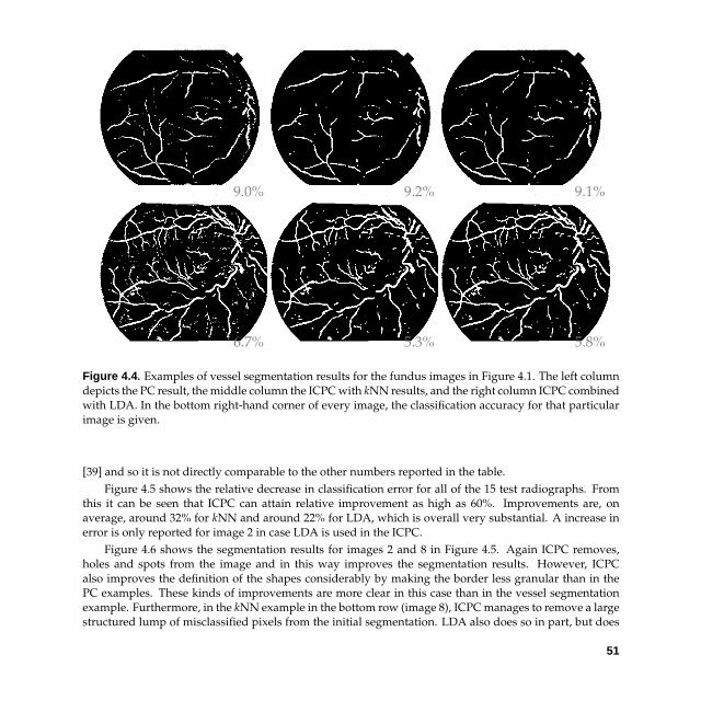
9.0% 9.2% 9.1%

6.7% 5.3% 5.8%

Figure 4.4 . Examples of vessel segmentation results for the fundus images in Figure 4.1. The left columndepicts the PC result, the middle column the ICPC with kNN results, and the right column ICPC combinedwith LDA. In the bottom right-hand corner of every image, the classification accuracy for that particularimage is given.

[39] and so it is not directly comparable to the other numbers reported in the table.Figure 4.5 shows the relative decrease in classification error for all of the 15 test radiographs. From

this it can be seen that ICPC can attain relative improvement as high as 60%. Improvements are, onaverage, around 32% for kNN and around 22% for LDA, which is overall very substantial. A increase inerror is only reported for image 2 in case LDA is used in the ICPC.

Figure 4.6 shows the segmentation results for images 2 and 8 in Figure 4.5. Again ICPC removes,holes and spots from the image and in this way improves the segmentation results. However, ICPCalso improves the definition of the shapes considerably by making the border less granular than in thePC examples. These kinds of improvements are more clear in this case than in the vessel segmentationexample. Furthermore, in the kNN example in the bottom row (image 8), ICPC manages to remove a largestructured lump of misclassified pixels from the initial segmentation. LDA also does so in part, but does

51

Table 4.3 . Overview of lung field segmentation results. Opening gives the accuracy of the segmentationobtained by opening the PC results with a disc of diameter 5. The maximum prior classifier assigns allpixels to the class having the maximum prior probability. The p-values reported are based on a pairedt-test.

type of segmentation p-value average relativesegmentation error decrease in error

pixel classification 3.3% — —ICPC (kNN) 2.1% 6 · 10−4 32%ICPC (LDA) 2.4% 1 · 10−3 22%2nd observer 1.6% — —

opening 2.9% — —maximum prior 23.0% — —

2 4 6 8 10 12 14−20

−10

0

10

20

30

40

50

60

70

images

rela

tive

decr

ease

in c

lass

ific

atio

n er

ror

(in

%) kNN

baseline

2 4 6 8 10 12 14−20

−10

0

10

20

30

40

50

60

70

images

rela

tive

decr

ease

in c

lass

ific

atio

n er

ror

(in

%) Fisher LDA

baseline

Figure 4.5 . Plots of the relative decrease in classification error for the 15 test posteroanterior chest radio-graphs. The left plot presents the results using ICPC with the kNN classifier and the right plot presentsthe results using LDA.

52

not succeed completely. A clear difference in the resulting ICPC segmentations is that the kNN preservessharp corners nicely, while the LDA scheme rounds the corners to a great extent.

1.5% 1.3% 1.7%

5.7% 2.2% 3.9%

Figure 4.6 . Examples of lung field segmentation results for the chest radiographs in Figure 4.2. The leftcolumn depicts the PC result, the middle column the ICPC with kNN results, and the right column ICPCcombined with LDA. In the bottom right-hand corner of every image, the classification accuracy for thatparticular image is given.

4.3 Discussion

The experiments in the previous section show that ICPC is capable of significantly outperforming pixelclassification. Although visually the vessel segmentations using ICPC may not necessarily look moreappealing than the PC results, there is a clear improvement obtained when it comes to segmentation

53

accuracy in terms of correctly classified pixels. Looking at the results from the lung field segmentations,the impact of of ICPC is unmistakable, particularly when using ICPC based on the kNN classifier. In theexamples shown in Figure 4.6, it is obvious that small and large scale noise has been removed and thelung shapes are more well-defined after applying several contextual reclassification steps.

Classifier design + contextual class label modelling

Of course, although the PC scheme was tuned quite carefully, it may be possible to improve it such thatits performance comes closer to the ICPC results, making any additional ICPC iterations superfluous.However, using these PC results as the initial segmentation for subsequent iterations, the ICPC resultsmay also be improved to further extent1. In addition, using ICPC it is probably easier to control the par-ticular class label configurations in the final segmentation so to fulfill certain requirements, e.g. smoothobject boundaries. Though neither when using PC nor ICPC, it would be straightforward to design suchclassification schemes (cf. [44]). An example of such possible requirement is illustrated by the lung seg-mentation results. Using ICPC the lung boundaries are particularly well defined and it seems hard tomake a PC produce such smooth delineations in a single pass as there will always be pixel misclassifiednear the borders.

Generally, the success of ICPC, like that of PC, depends on the performance of the classifiers used.Designing proper classifiers for ICPC may not be an easy task, but it is not necessarily more difficult thanclassifier design as encountered in other problems formulated as pattern recognition or machine learningtasks. It is actually, one of the strengths of ICPC that it allows the user to employ the complete collectionof standard pattern recognition and machine learning tools.

There is one particularity of the ICPC method that might complicate matters slightly and that is theway the contextual class label information is encoded. In the current work, this is done by encodingevery class label that is part of the class context N(i) as a K-dimensional (K is the number of classes)0/1-feature vector. As sN(i) is a concatenation of all these K-dimensional feature vectors, within a certainneighborhood of the central pixel pi , it tends to become very high dimensional for large neighborhoods.

A possible way to deal with such high-dimensional representations is to reduce the dimensionality ofthis feature vector prior to training the classifier. In the two examples in Section 4.2, we simply used PCA,which is an unsupervised technique. However, supervised schemes similar to LDA [22, 37, 47] seem moreappropriate and may proof to perform better (see also Chapters 1 and 2).

A more elegant—and possibly more efficient—approach to modelling the contextual class label in-formation is the following. One can think of the K-dimensional 0/1 label vectors κ as being representedby means of K binary images (having the same size as the original image L), i.e., for pi , the first imageholds the first entry of κ at position i, the second image the second entry in the same position i, etc. Con-sequently, the pixel values in the jth image are 1 if they belong to class j and 0 otherwise. The featurevectors sN(i) can easily be constructed by taking from all K images the pixel values from the neighborhood

1For a illustrative example of the capabilities of ICPC when using more carefully designed features for the task athand, we refer to the work described in Chapter 5.

54

N(i). This results in essentially the same contextual class feature vectors sN(i) as used in the experiments.However, similar to constructing gray value features, instead of taking raw pixel values, one can alsoapply various filters to the K binary class-indicator images and take these filter output as the features todescribe the class contextual information of the pi . Besides that the foregoing approach enables one tomodel the contextual information with fewer features, it also models the label information more insight-ful and natural—e.g. not based on pixels [34], and it can deal more easily with, for example, image sizechanges simply by changing the scale of the filters accordingly.

Cliques versus features

As mentioned in the Introduction, using ICPC, one avoids the clique formulation as employed in mostof the Markov random field formulations. Besides that statistically modelling all these cliques properlymight be complicated, another drawback is that the number of cliques grows very rapidly as the size ofthe neighborhood increases. In addition, the situation obviously worsens with increasing image dimen-sionality. This problem could for example be remedied in part by merely modelling pairwise interactions,but still the complexity of the model grows rapidly when neighborhood size increases.

On the other hand, as discussed in the previous subsection, modelling the contextual label informa-tion via a concatenation of K-dimensional 0/1-feature vectors κ also leads to an increasingly complexproblem as the neighborhood size grows. In this case, at a certain point, the dimensionality of this featurespace may become a limiting factor in applying the ICPC framework. The previous subsection discussestwo possibilities to overcome or avoid the problems related to the high-dimensionality of the featurespace: Performing a dimensionality reduction of this space or modelling the contextual label informationusing filter outputs.

All in all, it is clear that modelling the label context via a feature vector representation is not directly asolution to the problems related to context modelling through cliques. It is more a view on the contextualmodelling problem that may be preferable for certain kinds of tasks. Maybe even more so, it may be amatter of taste which approach is preferred.

Further improvements + extensions

We end this section with some additional suggestions for possible improvements and extensions to thebasic ICPC framework.

� The classifier used during the iterative part takes as part of the input the vectors sN(i) which possi-bly are noisy and incorrect and can change due to the reclassification of labels in the vicinity of pi .However, the classifier is trained using vectors sN(i) directly coming from the training segmenta-tions. These training contextual label vectors contain therefore the correct labellings and so there isa discrepancy between the vectors that are to be classified and the vectors the classifier was trainedon.

55

To deal with this discrepancy, similar to a suggestion made in [24] for the recurrent sliding win-dows technique, one could train a new classifier for every iteration in ICPC using the training data.More precisely, the training procedure would be as follows:

1. Train a classifier, using feature vectors xi , and obtain an initial segmentation of the trainingimages using this classifier.

2. Train a new classifier, using the segmentations coming from the previous step—from whichthe vectors sN(i) are extracted—and again the feature vectors xi from the train images them-selves, and update the training image segmentations using this classifier.

3. Repeat from step 2 until convergence or some other stoping criterion is fulfilled.

This training procedure results in a sequence of classifiers that can then be (sequentially) appliedto test images to produce their segmentations.Obviously, though this procedure may be more powerful than the original ICPC formulation, it isalso much more involved and may therefore be, especially if a long sequence of complex classifiersis needed, impracticable in many real-world situation in which one has to deal with large data sets.An intermediate solution is to construct a sequence with a small number of classifier and use thelast classifier in the sequence repeatedly in the final iterations.

� In the ICPC iterations, the relabelling of pi is based on the feature vector fi . This vector combinesfeatures of very different type: Image features from xi that are continuous and contextual classlabel features from sN(i) that are discrete.Instead of building a single classifier that deals with fi in its totality, it can be beneficial to builtseparate classifiers for xi and sN(i), that are able to deal well with the specific types of features, andto use a classifier combination scheme [55, 64, 129] to afterwards combine the classification resultsobtained with the two specialized classifiers. In Chapter 5, we actually follow this approach anduse a product rule on the posterior probabilities of the two classifier outputs.

� A final extension of ICPC that could lead to improvements concerning performance accuracy andcomputational burden, as well as, classifier and feature design, is to link ICPC to a multi-scaleand/or hierarchical framework. Within the field of Markov random field theory several suchframeworks have been developed and studied (see for example [9], [69], and [126]), and we maydraw from these theories to convert the present data-driven discriminative image segmentationscheme into a multi-scale/hierarchical one. Such extension may, for example, enable the use ofICPC on large 3-dimensional or 4-dimensional (medical) image data sets while this may not befeasible with the original ICPC formulation.

4.4 Conclusions

We have presented a general, pixel-based, data-driven and discriminative segmentation approach callediterated contextual pixel classification (ICPC). The most important feature of our method is that it utilizes

56

standard supervised pattern recognition and machine learning techniques to learn the image segmen-tation task and to exploit contextual information present in neighboring class labels. The approach canconsidered to be a supervised version of Besag’s iterated conditional modes providing a suboptimal so-lution to the segmentation task formulated in terms of a maximum a posteriori optimization problem.

Through experiments on two real-world image segmentation tasks, it has been shown that ICPCsignificantly outperforms supervised pixel classification and comes close to the accuracy obtained by asecond observer. Besides that, in certain cases, it has also shown to improve the visual appearance ofthe segmentations by enhancing the coherence of the segments and creating more clearly defined objectboundaries.

Finally, in an extensive discussion, we have indicated several interesting extensions and possibleimprovements all of which be captures within the same basic ICPC framework.

57

58

5

Segmentation of the Posterior Ribsin Chest Radiographs

using Iterated Contextual Pixel Classification

Computer analysis of chest images for computer-aided diagnosis (CAD) can benefit from an accuratedelineation of the rib cage, which makes this segmentation task of great practical importance. Preciseidentification of the ribs can aid in the detection of rib lesions and the localization of lung lesions [68,45]. In general, ribs are often used as a suitable frame of reference within the lung fields and once asegmentation is available, such a reference frame could be benefitted from in further computer analysisof the chest. Furthermore, delineation may, for example, lead to a decreased number of false positivefindings in computerized detection of abnormalities, because such findings are often located on crossingsof posterior and anterior ribs, and hence to an overall improvement of a CAD system for X-ray chestradiographs.

Segmentation of the ribs in projection X-rays is a difficult task. The superimposition of, for the task,irrelevant anatomical structures such as thoracic vasculature, clavicles, the heart, and fatty tissue can makeit hard to distinguish the edges corresponding to rib borders. The acquisition of PA chest radiographs isoptimized for visualizing thoracic structures instead of bony anatomy. When the bone mineral densityis low, which is common in elderly patients and in the lower ribs, rib borders can even be completelyinvisible. Anatomical knowledge about the rib cage is guiding human observers in rib detection in thosecases.

We have developed iterated contextual pixel classification (ICPC, see [81] and Chapter 4) for complexsegmentation tasks such as the one at hand. ICPC is a general, supervised (i.e, manual segmentationsshould be provided for training) segmentation algorithm which uses techniques from statistical patternrecognition. It can be used when it is not clear how to provide a global shape description, and tech-niques like active shape or active appearance models [17] cannot be readily applied. In the case of ribsegmentation, the variable number of visible ribs in the lung fields complicates the use of a global shapemodel.

The evaluation of the method, in Section 5.3, is performed on 30 digitized 512 × 512 chest imagestaken from the publicly available JSRT (Japanese Society of Radiological Technology) database [115].

Relation to previous work

Most methods for rib segmentation use a geometrical model of a rib or the rib cage. Ribs have beenmodelled as parabolas [125, 110] or ellipses [116, 108], and the ribcage as a sinusoidal pattern [97, 108].These models have been fitted, usually with a modified Hough transform, to the image data directly,to edges extracted from the lung fields, or to morphologically processed images [110]. To remove falseresponses, or infer missing borders, rule-based reasoning schemes have been proposed [125, 131]. In [131]snakes were used for additional refinement of the rib border. In [43] a statistical model of the completerib cage has been constructed and fitted to edge information. Except for the rib cage shape model in [43],none of these approaches were supervised.

Our approach to the rib segmentation task is different from the ones above. ICPC is principally pixel-based, supervised, and no global or geometric model is taken into account. However, it does exploitstructural information that is present in the training data, and uses this information to come to a goodsegmentation locally. Hence it avoids, as pointed out earlier, problems that global models may sufferfrom. Section 5.4 offers more discussion on this topic.

Finally, it is noted that a rib segmentation approach comparable to the one presented here, which alsouses ICPC, was described by the authors in [85]. The current work extends and improves upon the latterreference and offers a more extensive validation of the method.

Outline

Section 5.1 presents the materials on which the experiments are performed. Section 5.2 introduces theICPC method, emphasizing the specific setup for tackling the rib segmentation problem. Section 5.3presents the results of the experiments conducted to validate our method. Finally, Section 5.4 providesthe discussion and concludes this chapter.

5.1 Materials

The data used to test our approach to rib segmentation consists of 30 digitized, standard PA chest radio-graphs that are taken from the JSRT database, which is a publicly available chest radiograph database[115]. 15 of them were taken randomly from the 154 containing a nodule and the other 15 were takenrandomly from the remaining 93 normal cases. The size of all original images equals 2048 × 2048. Forour method we sub-sampled these images to 512× 512 pixels. An example of such a radiograph is shownin Figure 5.1.

For this study, two human observers have manually segmented the ribs within the lung fields in eachof these images independently. Both observers (the first author and a medical computer science student)received instructions from an experienced radiologist. The radiologist was consulted in case of doubtwith respect to the right segmentation. Segmentation was performed with a mouse device, using a toolthat allowed zooming and window levelling. Time available was not limited, segmentation required onaverage 25 minutes per image. A segmentation performed by the first observer is shown in Figure 5.1.

60

Figure 5.1 . Left: Radiograph from the JSRT database used in the evaluation of the ICPC segmentationmethod. Middle: Manual segmentation provided by the first observer. The costal space is in white,intercostal is gray. Right: Second observer’s manual segmentation.

The observers only delineated the posterior ribs within the lung fields. The delineation of the lung fieldsis assumed to be given. Automatic segmentation of lung fields can be done efficiently using, for example,an active shape model approach [40].

The per-image pixel-based performances over the thirty radiographs of the second observer are cal-culated taking the first observer as the one providing the gold standard. The performances are calculatedwithin the given lung fields. For these scores, we subsequently determined the mean and standard de-viation (s.d.) over the 30 images. The results are as follows (the s.d. is in parentheses): Accuracy 0.94(0.02), sensitivity 0.92 (0.03), and specificity 0.95 (0.02). The accuracy, sensitivity, and sensitivity are alldetermined on a per pixel-basis in which pixels being labelled as costal are taken to be positive and pixelsbeing labelled intercostal are negative. Comparing a segmentation to the gold standard, based on thenumber of pixels being true positives (TP), false positives (FP), true negatives (TN), and false negatives(FN), the accuracy can be determined as TP+TN

TP+FP+TN+FN . Using the same notation, the sensitivity equalsTP

TP+FN and the specificity is given by TNTN+FP . These are the quantities with which we shall evaluate the

performance of ICPC.

5.2 Iterated Contextual Pixel Classification

This section starts with some definitions. Let L be an image consisting of n pixels. Define s = (s1 , . . . , sn) tobe a vector of length n, containing the class labels si belonging to image pixel pi . The complete vector s oflabels is the actual segmentation of L. Class labels are in the set C = {c1 , c2 , . . . , cl}, where l is the numberof classes. Pixels having the same label are in the same segment of the image. In chest radiography, the setC could consist of anatomically motivated classes like left lung, posterior rib, heart, etc., but also classes

61

for particular diseases and/or abnormalities may be incorporated.The problem of finding an optimal segmentation s of an image L, is initially defined in terms of a

maximization of the posterior probability P(s|L), which is the probability of having s as a segmentationof the image L. The optimal segmentation s? is the one that maximizes this probability, i.e.,

s? = argmaxs∈Cn

P(s|L). (5.1)

ICPC provides an approximation to s? by iteratively updating the labelling of single pixels. This localupdating of the segmentation is based on two kinds of (local) features which are associated to the pixelspi . These features are referred to as image features and context features.

Subsection 5.2 introduces the former features, the image features, as used in the rib segmentation task.Subsection 5.2 discusses the pixel classification procedure used to obtain the initial image segmentationbased on these image features. Subsequently, the general idea behind ICPC is elaborated on in Subsec-tion 5.2, which clarifies the need for the latter kind of features, the context features. Subsection 5.2 thendescribes the context features used in the current segmentation task and Subsection 5.2 presents the ICPCreclassification procedure that employs both image features and context features. Finally, Subsection 5.2recapitulates the ICPC approach and concludes with some additional remarks.

Image features

Examples of image features that can be used in an image segmentation task are the gray value in a pixel,the gray values of its neighboring pixels, the output of filters, statistics from a neighborhood around thepixel, or the position in the image. Of course, many other features are possible based on different imagecharacteristics. For the rib segmentation task, the choice of features1 was restricted to raw gray levels andcertain Gaussian filter outputs as described below. However, to begin with, before extracting the actualimage features, images are locally normalized at scale 16 to remove gross intensity variation within andbetween images, i.e, the initial image L is transformed to

L =L − Lσ√

(L2)σ − (Lσ )2,

where Lσ is the image L blurred with a Gaussian with scale σ . In our case, σ = 16.Per pixel, image features were subsequently extracted from L using Gaussian filters at scales 1, 2, and

4 and their derivatives up to order 2. Additionally, the raw gray value of the pixels in L is taken as afeature. Other natural features, like the raw pixel coordinates, are not taken into account, as they did notgive any significant increase in performance of ICPC. Hence the image features consist merely of graylevel information. We denote the feature vector associated with pixel pi by xi . In the rib segmentation

1This particular choice of features as well as other choices presented in the remainder of the chapter—concerning theclassifiers used and the parameters that need to be set—are based on pilot experiments using 25 images as training dataand 1 or 2 images to study the resulting segmentations. In any case it holds that slight variations of the parameters didnot yield solutions that are significantly different from the ones presented here.

62

approach presented, its dimensionality d equals 19, i.e., there are six derivatives (one zeroth order, twofirst order, and three second order) at three scales plus one extra dimension for the raw gray value in thepixel.

Subsequently, the feature vectors are reduced in dimensionality by means of a linear feature extrac-tion technique ([37, 55]) presented in [78, 79]. This technique, which is a extension of Fisher’s lineardiscriminant analysis [37, 55], is designed to cope with distributions in which classes do not necessar-ily have equal covariance matrices. It is based on basic matrix manipulations and the Chernoff distancemeasure [13, 14], and comes down to determining an eigenvalue decomposition of the matrix

S−1W (SB − S

12W(π1 log(S

− 12

W S1S− 1

2W )

+π2 log(S− 1

2W S2S

− 12

W ))S12W) .

(5.2)

In Equation (5.2), SB := ∑2i=1 πi(mi − m)(mi − m)T and SW := ∑2

i=1 πiSi are the between-class andthe average within-class scatter matrix, respectively; mi is the mean vector of class i, πi is its a prioriprobability, and the overall mean m equals ∑2

i=1 πimi . Furthermore, Si is the within-class covariancematrix of class i.

Note that the term S12W(π1 log(S

− 12

W S1S− 1

2W ) + π2 log(S

− 12

W S2S− 1

2W ))S

12W takes care of the difference in

the covariance matrices of the two classes. If there is no difference present, this term becomes zero and thematrix in (5.2) reduces to S−1

W SB, which is related to the Fisher criterion associated with linear discriminantanalysis [37]. It has been shown that this feature extraction technique increases the performance in severalother classification problems [78, 79].

For the current segmentation task, the 19-dimensional feature vectors are reduced to 13 dimensionsby transforming them by the 13 × 19 linear transformation matrix L. The rows of this matrix equal the13 19-dimensional eigenvectors corresponding to the 13 largest eigenvalues and obtained through theeigenvalue decomposition of the matrix in Equation (5.2).

Pixel classification

The initial segmentation of an image L that is used by ICPC is obtained by a classification of the pixelsbased on the image features, i.e., for every pixel pi , si takes on the class label c ∈ C that maximizesP(si = c|xi). Many supervised approaches are know from the literature to come to such a classification,see for example [37, 55].

For the rib segmentation task, to perform this initial classification, a k-nearest neighbor classifier (k-NN) [37, 55] is employed. Mount and Arya’s tree-based k-NN implementation [91], allows for a speedup of the classification, without much loss of accuracy, by calculating an approximate solution. The ap-proximation variable ε is set to 1, which means that the (1 +ε)-approximate nearest neighbors, which thealgorithm finds, are no more than double the distance away from the query point than the actual nearestneighbors are (see [2]). In the experiments, only one in every 64 feature vectors is used for building theclassifier (the training) and the number of neighbors (k) to be found is set to 63.

63

This initial segmentation phase is called pixel classification (PC), which provides a simple supervisedapproach to image segmentation.

The ICPC algorithm

This subsection turns back to the problem statement in the beginning of this section and considers the op-timization in Equation (5.1) more closely. These considerations lead to the proposal of the ICPC algorithmto approximate the optimal solution s?. As becomes clear in the following, ICPC improves upon PC bytaking structural information into account in addition to image gray value information. This structuralinformation is encoded in the second kind of features: The context features.

Consider two segmentations, s and σ , of L that merely differ from each other in one single entry, say,the ith—belonging to pixel pi , then, using Bayes’ theorem, it can be shown that

P(s|L)P(σ |L)

=P(si |σ¬i , xi)P(σi |σ¬i , xi)

, (5.3)

where s¬i is defined as the vector (s1 , . . . , si−1 , si+1 , . . . , sn). Note that the last equivalence is obtained byassuming that in order to label si and σi , the only information needed from the image L is present in the(local) image feature vector xi—an assumption that is implicitly present in the PC approach as well. Thisassumption is similar to the well-known Markov assumption in Markov random field theory [8, 127].

Now, assuming that all probabilities P(s|L) are larger than zero, it follows from (5.3), that P(s|L) >P(σ |L) if and only if

P(si |σ¬i , xi) > P(σi |σ¬i , xi). (5.4)

Hence, if P(s|L) > P(σ |L), accepting segmentation s in favor of σ , would give us a segmentation that iscloser to the optimal s?. Note that the decision, whether s is better or worse than σ , can be based solely onthe comparison of the conditional probability in (5.4) for the single ith entry. The basic idea with respectto this local update step, i.e., in going from labelling σi to si or, similarly, from segmentation σ to s, is thatone chooses that class label for si that maximizes the aforementioned conditional probability P(si |σ¬i , xi).

Considering the foregoing, in the update step of ICPC, one always decides to have s as the newsegmentation, because it always holds that P(s|L) ≥ P(σ |L). ICPC enforces an increase in global posteriorprobability based on local decisions. Interestingly, this update step can also be seen as a classification taskin which the extended feature vector (σ¬i , xi) is to be classified to one of the l classes in C. Bayesianclassification suggests that this extended feature vector (σ¬i , xi) should be classified to that class c forwhich P(si = c|(σ¬i , xi)) is largest (compare with PC in Subsection 5.2).

After an initial PC, the ICPC algorithm iterates the aforementioned procedure of changing one of thelabels of the segmentation σ and accepting the new segmentation s, if and only if Inequality (5.4) holds.It therefore leads to an approach which finds a locally optimal solution to Equation (5.1) (cf. [8] and [127])and generally improves upon merely using PC.

64

Context features

The extended feature vector from the previous section combines features describing contextual class labelinformation belonging to pixel pi with the previously introduced image features vector xi . However,similar to the approach dealing with the image features, it is assumed that not all entries in s¬i are relevantto the actual labelling of si and therefore only a limited set of neighboring labels are considered as contextfeatures. This context feature vector is denoted vi for every pixel pi .

N.B. The class labels of the si , of which the contextual feature vector is built up, are categorical, ratherthen numerical. Most classifiers, however, can only handle numerical feature vectors. This is solved byassociating a label c j with a jth standard basis vector in l-dimensional Euclidean space, i.e., associate c jwith (0, . . . , 0, 1, 0, . . . , 0), where the jth entry equals 1. The context feature vectors vi are therefore builtup of such standard basis vector.

For the current segmentation task, the contextual class label features vi come from the class labels ofpixels within a 176 pixel radius from the pixel to be reclassified. However, not all labels within this radiusare used. Labellings that are close to pi are generally more important than labellings further away. Forthat reason, the labellings away from pi are more sparsely sampled than those close to the central pixel.For the rib segmentation, the relative coordinates (i, j)—i.e., (0, 0) is the central pixel—of contextual classlabels taken into account, are constructed as follows.

1. Determine all integer pairs (a, b) 6= (0, 0) for which a2 + b2 ≤ 64 (there are 196 of such pairs)

2. Calculate the relative class label feature coordinates (i, j) by setting

i = ba · exp(0.3√

a2 + b2) + 12 c

andj = bb · exp(0.3

√a2 + b2) + 1

2 c ,

where b·c gives the floor of a real number.

Figure 5.2 gives an impression of the spatial distribution of the resulting 196 class label feature coordi-nates.

Only the pixels within the lung fields are to be segmented (into costal or intercostal), and therefore itis a two-class classification problem. However, there are three classes to be represented because the neigh-borhood of a certain lung field pixel can overlap with the background, which makes up the third class.Henceforth, the set of class labels C for representing the contextual class label features is {background,costal, intercostal}.

Like the image feature vector, the dimensionality of the context feature vector vi is also reduced. Tothis end, a principal component analysis (PCA, [37]) is used. As opposed to the dimensionality reductionemployed for the gray level data, the PCA is solely done for speeding up the iterative segmentationprocedure. (A dimensionality reduction by means of the Chernoff criterion or LDA did not give anyimprovement over the results obtained.) In the initial class label feature space, the lower-dimensionalsubspace is determined that retains 90% of the variance in the data. In the cross validation experiments,presented in Section 5.3, this comes down to using about 140 class label features in every run.

65

−90 0 90

−90

0

90

Figure 5.2 . Positioning of the 196 relative coordinates used for determining the context features. Thesampling of the label features is sparser as one is farther away from the central pixel, i.e., the pixel to berelabelled. The diameter of the contextual region is 176 pixels.

66

ICPC reclassification

Like in the initial PC step, in the subsequent ICPC steps the pixels are to be classified based on certainfeatures. The main difference being that these additional ICPC steps also take structural information intoaccount by dint of the feature vectors vi . Because one is dealing with a different feature vector in the lattersteps, i.e., an extended feature vector combining xi and vi , a classification scheme different from the oneused for PC should be employed. In general, a single classifier based on the complete extended featurevector (vi , xi) could be constructed and used in the ICPC algorithm. However, to cope with the differenttypes of features involved in the classification task, a classifier combination scheme based on the productrule is used [55, 64] (cf. [61]). The posterior probabilities P(si = c|vi) and P(si = c|xi), for all possiblelabels c ∈ C, are estimated and combined afterwards via the following rule:

P(si = c|(vi , xi)) = P(si = c|vi)P(si = c|xi).

Reclassification takes place based on the quantity above which gives estimates proportional to the classposteriors of the extended feature vector (vi , xi). Note that generally the products P(si = c|vi)P(si = c|xi)do not add up to 1. However, for the final classification, one is merely interested in the relative magnitudesof the posterior probabilities, as this is sufficient to decide to which class a sample belongs: The pixelshould be relabelled to the class producing the largest resulting product.

P(si = c|xi) is obtained from the 63-NN classifier from Subsection 5.2. Generally, given an k-NN clas-sifier, posterior probabilities can be obtained by determining, among the k-nearest neighbors, the numberk j of samples belonging to class c j and setting (see [61])

P(si = c j|features) =k j + 1k + l

.

In our case l, which is the number of classes in which to classify, is 2.

In addition, based on the context features as described in the previous section, a k-NN with k set to101 is built. Again, Mount and Arya’s tree-based k-NN implementation is used with ε set to 1. Now, fora certain pixel pi that is to be reclassified, using the 101-NN classifier, a posterior probability P(si = c|xi)can be established as well and therefore the resulting product can be determined. Note that for the imagevectors xi , the posterior probabilities have to be determined only once and can be stored during the initialpixel classification after which all P(si = c|xi) are known. The P(si = c|vi) have to determined everytime a pixel is to be reclassified because the context features in vi may have changed, which influences theposterior.

Finally, it is noted that the product rule is a sensible choice when the gray level and contextual classlabel representation can be assumed to be statistically independent of each other. Although this may notbe true to the full extent, it is an assumption commonly made [8] and it turns out to work well for ourpurpose.

67

Interlude: Recapitulation + some accompanying remarks

Before continuing our exposition, the general ICPC algorithm is recapitulated and some remarks aremade.

In brief, ICPC comes down to the following iterative scheme:

1. Start with a pixel classification (PC) based on the image feature vectors xi ; this gives an initialsegmentation of the image.

2. Iteratively update the current pixel class labels si in s:

(a) Go over all pixels pi .

(b) Reclassify every pixel based on both the image feature vector xi and the context feature vectorvi . The latter can be extracted from the intermediate segmentation, while the former is thesame as for the initial PC.

(c) Repeat from 2a unless, for the whole image, no relabelling has occurred or a maximumnumber of iterations is reached.

The following remarks supplement the foregoing.

� There are two classifiers needed in this method, which are both to be trained from training data.One is used for the initial segmentation of L using only the image features in xi (the initial pixelclassifier, Subsection 5.2), and a second one reclassifies pixels based on both xi and the structuralinformation present in the context feature vectors vi (Subsection 5.2).In the rib segmentation task two two-class classifiers are involved, that, based on the product rule,(re)classify pixels into either costal or intercostal.

� A visiting scheme has to be chosen, defining the order in which the pixel locations in the image aretraversed. There are several possibilities, deterministic as well as stochastic.In our segmentation scheme, a stochastic pixel visiting scheme is used to traverse all pixels in thelung fields. During a single iteration, the algorithm goes through a random list of all coordinates inthe image. Pixels are only eligible for reclassification if they meet the following two requirements:

1. The pixel is lying next to the edge of a segment. This is done by checking whether the fivelabels in the 4-neighborhood of the central pixel are equal or not. Edge pixels are typicallyprone to be relabelled

2. There has been a change in the context features of the central pixel since it has been visitedfor the last time, i.e., one or more of the class labels in its neighborhood have changed sincethe last visit.

These requirements avoid the reclassification of too many pixels of which it is not likely that theychange their label at that point in the iterative scheme. Because reclassification is the computation-ally most expensive stage of the algorithm, verifying the criteria above reduces segmentation timeconsiderably.

68

� A stopping criterion is needed, because the iteratively updated segmentation may not converge.Convergence is not guaranteed, because the Markov property may not hold and/or the statisticalmodel used is not consistent with the Markov model assumption.

In the current scheme, the segmentation is stopped if a maximum number of 50 iterations has beenmade or if there were no changes in the labelling during a full iteration. This maximum numbersuffices for the posterior rib segmentation in all cases.

5.3 Experiments, Results, + Evaluation

Cross validation results

Six-fold cross validation experiments are performed to evaluate the performance of the ICPC approach onthe rib segmentation problem, i.e., our method is trained on 25 images, tested on the other five, and this isrepeated six times for different training and test sets with the constraint that every image is only part of thetest set once. It is noted here that the training based on the 25 training images merely involves determiningthe optimal CLDA and PCA feature extractions and building both k-NN classifiers. The parameters andfeatures chosen are fixed throughout all of the cross validation experiments. The latter also holds for thedimensions to which the image feature vectors (Subsection 5.2) and the context feature vectors (Subsection5.2) are reduced to, and for the k parameter of the image feature k-NN classifier (Subsection 5.2) and thecontext feature k-NN classifier (Subsection 5.2). These four parameters are fixed to 13, 140, 63, and 101,respectively.

The segmentation is restricted to the lung fields, with merely two classes into which these pixels canbe classified: Posterior rib (the costal space) or not (the intercostal space). Although this means that a pixelshould only be classified into one of the two aforementioned classes, the third class (background) shouldstill be taken into account when constructing the context feature vector vi . This structural informationmay still include background because the contextual neighborhood of a pixel within the lung fields mayoverlap with the background.

On the test set, the per-image pixel-based accuracy, sensitivity, and specificity obtained by ICPC is de-termined (relative to the delineation of the first observer). The mean and standard deviation (s.d.) of thesethree entities is then calculated over the 30 images. The results are in Table 5.1. In this table, the scoresof the initial PC scheme are also given, that is, the segmentation obtained without the additional contex-tual label reclassification steps. This shows the improvements possible by incorporating contextual labelinformation into the segmentation. Additionally, the results when using a global automatic segmentationmethod, as presented in [43], are also provided in the table.

Average segmentation times for ICPC, PC, and the second observer are approximately 12, 0.5, and25 minutes, respectively. The segmentation methods are run on standard personal computer with a 2.8GHz processor. The previous numbers are merely meant to give an indication of the orders of magnitudeof the times needed to perform a single segmentation. Generally, they can highly vary from observer toobserver and from implementation to implementation.

69

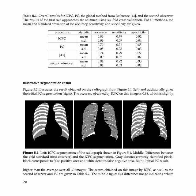
Table 5.1 . Overall results for ICPC, PC, the global method from Reference [43], and the second observer.The results of the first two approaches are obtained using six-fold cross validation. For all methods, themean and standard deviation of the accuracy, sensitivity, and specificity are given.

procedure statistic accuracy sensitivity specificity

ICPCmean 0.86 0.79 0.92s.d. 0.06 0.09 0.04

PCmean 0.79 0.71 0.85s.d. 0.05 0.08 0.03

[43]mean 0.74 0.79 0.77s.d. 0.09 0.07 0.07

second observermean 0.94 0.92 0.95s.d. 0.02 0.03 0.02

Illustrative segmentation result

Figure 5.3 illustrates the result obtained on the radiograph from Figure 5.1 (left) and additionally givesthe initial PC segmentation (right). The accuracy obtained by ICPC on this image is 0.88, which is slightly

Figure 5.3 . Left: ICPC segmentation of the radiograph shown in Figure 5.1. Middle: Difference betweenthe gold standard (first observer) and the ICPC segmentation. Gray denotes correctly classified pixels,black corresponds to false positive area and white denotes false negative area. Right: Initial PC result.

higher than the average over all 30 images. The scores obtained on this image by ICPC, as well as thesecond observer and PC are given in Table 5.2. The middle figure is a difference image indicating where

70

Table 5.2 . Results for ICPC, PC and the second observer on a typical image, i.e., one for which the ICPCaccuracy is close to the overall mean ICPC accuracy. Given are the accuracy, sensitivity and specificity.

accuracy sensitivity specificityICPC score 0.88 0.83 0.92

PC score 0.81 0.75 0.86second observer 0.94 0.93 0.95

the differences between the first observer’s segmentation and the ICPC segmentation occur. The correctlyclassified pixels—the true positives (TPs) and negatives (TNs)—are in gray, the false positives (FPs) areblack and the false negatives (FNs) are white.

From the example it is clearly visible that, if there are errors, they are present in a structured way.Falsely classified pixels are not scattered around in the segmentation image—as is the case in the pixelclassified image, but they tend to occur in regions elongated in the direction of the ribs. Note that ICPCmissed the lowest ribs in both lungs completely, although it appears that the initial PC at least gave asmall indication that there is a rib present at that location in the right lung.

Poorest ICPC result

To illustrate more extensively the kind of errors ICPC can make, Figure 5.4 gives the radiograph, thedelineation by the first observer and the ICPC result associated to the poorest segmentation result. Thethree most obvious errors from this image are

1. Ribs are segmented only partly (left and right lung field)

2. Ribs can vanish completely (left and right lung field)

3. The clavicle is mistaken for a rib (left lung field).

For comparison, the scores obtained by the second observer, ICPC and PC are in Table 5.3. Note that inthis case segmentation accuracy by PC is higher than the ICPC accuracy.

Region dependent performance

We expect the segmentation results—of ICPC as well as the human observer—to depend on the regionwithin the lung fields. To substantiate this expectation the lung fields are divided in several areas withinwhich the accuracy, specificity, and sensitivity are determined. These areas are obtained by using a simpleautomatic scheme which combines filtering, thresholding, and morphological operations, and applyingthat to the given lung field segmentations in such a way that, for every image, the top, middle, and lowerarea have approximately the same size. The following regions are distinguished (see Figure 5.5): The top

71

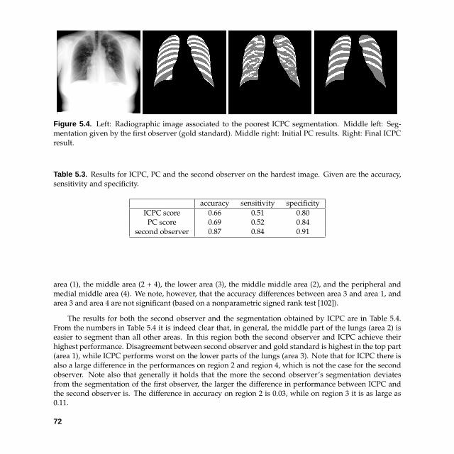
Figure 5.4 . Left: Radiographic image associated to the poorest ICPC segmentation. Middle left: Seg-mentation given by the first observer (gold standard). Middle right: Initial PC results. Right: Final ICPCresult.

Table 5.3 . Results for ICPC, PC and the second observer on the hardest image. Given are the accuracy,sensitivity and specificity.

accuracy sensitivity specificityICPC score 0.66 0.51 0.80

PC score 0.69 0.52 0.84second observer 0.87 0.84 0.91

area (1), the middle area (2 + 4), the lower area (3), the middle middle area (2), and the peripheral andmedial middle area (4). We note, however, that the accuracy differences between area 3 and area 1, andarea 3 and area 4 are not significant (based on a nonparametric signed rank test [102]).

The results for both the second observer and the segmentation obtained by ICPC are in Table 5.4.From the numbers in Table 5.4 it is indeed clear that, in general, the middle part of the lungs (area 2) iseasier to segment than all other areas. In this region both the second observer and ICPC achieve theirhighest performance. Disagreement between second observer and gold standard is highest in the top part(area 1), while ICPC performs worst on the lower parts of the lungs (area 3). Note that for ICPC there isalso a large difference in the performances on region 2 and region 4, which is not the case for the secondobserver. Note also that generally it holds that the more the second observer’s segmentation deviatesfrom the segmentation of the first observer, the larger the difference in performance between ICPC andthe second observer is. The difference in accuracy on region 2 is 0.03, while on region 3 it is as large as0.11.

72

Table 5.4 . Region dependent (see Figure 5.5) performance for second observer and ICPC.

second observer ICPCregion accuracy sensitivity specificity accuracy sensitivity specificity

1 0.92 0.90 0.94 0.84 0.81 0.882 + 4 0.95 0.93 0.96 0.89 0.86 0.92

3 0.93 0.90 0.94 0.82 0.61 0.932 0.96 0.94 0.97 0.93 0.89 0.954 0.94 0.93 0.95 0.87 0.83 0.90

5.4 Discussion + Conclusion

With respect to the pixel accuracy, sensitivity, and specificity, the results ICPC obtains are reasonablyadequate in comparison with a second observer, but, as Figure 5.4 shows, gross errors can be present inthe ICPC segmentation. Not all of these errors are typical though. Mistaking the clavicle for a rib, whichmay be considered the most severe one, occurs in only two out of 30 images. However, all images sufferfrom either only partly segmented ribs, or completely missed ribs. This almost exclusively happens in thelower regions of the lungs where the rib borders are often hardly discernable.

Other difficulties arise for the top part of the lung fields where the misclassification rate of ICPC isalso high (see Subsection 5.3). Besides the poor visibility of the ribs, an additional problem may be thatthe rib structures in the top of the lung are rather different and relatively small compared to the typicalstructures from the rest of the image. Hence, the statistical model may not capture these small structuresaccurately. It may be possible to improve performance by making the statistical model spatially varying,but this will probably require a much larger training set. In addition, as can be seen from the segmentationresults in Figures 5.3 and 5.4, the superimposition of the clavicles make the rib segmentation problematic.These bony structures are often more clearly visible than the ribs and, especially in the initial PC result inFigure 5.3, it is visible how they influence the segmentations. The confusion between ribs and clavicles isalso problematic in other methods, e.g. in [110].

Further, as noticed in Section 5.3, errors occur in a structured way in the segmentation and not, moreor less, randomly scattered through the entire image as is the case in the PC results. This is an inherentcharacteristic of our approach. Because of an imperfect contextual and gray level model, errors are madeduring the segmentation process. However, the contextual relabelling attempts to force the final segmen-tation to be consistent with the observed structures in the training set. Hence, errors are possible, but onlyin a structured way. In the rib segmentations obtained by ICPC, these structured errors become apparentas patches that are elongated in the direction of the posterior ribs, as if the complete rib is shifted one ormore pixels (see Figure 5.3).

A negative consequence of the foregoing is that if the initial pixel classified image is a very poor

73

segmentation, the ICPC result might get even poorer. No matter what the initial PC state is, ICPC triesto enforce a rib-like structure on it, which may be farther from the true segmentation than the initial(poor) PC segmentation. In our data set of 30 images this actually happened two times, and these twocases have also the lowest ICPC accuracy overall. Apparently, in these two radiographs, the gray levelfeatures provided not enough information for an adequate initial segmentation. In general, however,relabelling greatly improves upon the pixel classification result, and can correct even fairly large errors.An interesting example can be seen in Figures 5.1 and 5.3. In the middle part of the left lung (on the rightin the image) a pulmonary nodule is visible peripherally, just above a rib. Pixel classification mistakenlyidentified the nodule as rib, but after relabelling the region containing the nodule is correctly classified asintercostal space.

The errors that ICPC makes, such as partly segmented ribs, are possibly a result of too weak a struc-tural model: Although, there is no evidence in the training set for such an abrupt ending of a rib withinthe lung field, the (apparently misleading) gray level information is too strong—in comparison to thecontextual information—to have the context classifier correct the segmentation. In this case, increasingthe influence of the label context may improve the automatic segmentation.

Considering the aforementioned problems, we think improvements in accuracy can be attained byimproving the statistical model. This may be possible by using different features than the ones used here.If, for example, it is possible to combine the local gray level and context features with geometrical shape-based information, we might avoid the gross errors as seen and discussed in Section 5.3 and the foregoingparagraphs. In combination with our local pixel-based approach, a more global model may work welleven though such a model may not perform satisfactory when used in isolation. Further, Subsection 5.3shows that the performance varies drastically with the position in the lung fields. It may be possibleto improve results by taking into account the position relative to the lung field border—as opposed tosimply taking raw pixel coordinates, e.g. by using features based on a distance transform. Again, a largertraining set may be required to apply this successfully.

It is difficult to compare the performance of ICPC with previously proposed methods. Methodsthat use simple geometrical models are unlikely to achieve better performance as these models can onlyapproximate a true shape. The accuracy reported in [43] is well below the result of ICPC obtained here,which is also verified by our experiments in which the same system was used on our data. The only otherpublication that we know of that includes a quantitative evaluation [131] was tested on ten radiographsand used a different performance metric.

The computation time required for ICPC could be reduced by employing more clever stochastic visit-ing schemes. For example, based on posterior probabilities one could decide which pixels can be excludedfrom the visiting scheme and hence reduce the number of pixels that have to be considered for reclassifi-cation. Furthermore, multi-resolution schemes are currently being investigated. These schemes may alsogive improved performance with respect to the segmentation accuracy.

In conclusion, notwithstanding the problems and suggestions discussed in this section, the ICPCmethod presented clearly improves upon pixel classification and obtains good results on the difficult taskof segmenting the posterior ribs in chest radiographs.

74

11

33

44 4

42

2

Figure 5.5 . Example associated to the radiograph in Figure 5.1 of how the lung fields are divided intoseveral regions. Top area (1), middle area (2 + 4), bottom area (3), middle middle area (2), middle borderarea (4).

75

76

6

Suppression of Bony Structuresfrom Projection Chest Radiographs

by Dual Energy Faking

One of the major difficulties in interpreting projection chest radiographs stems from the fact that manynormal anatomical structures are shown superimposed on possibly abnormal structures. For this reason,many computer aided diagnosis (CAD) schemes in projection chest radiography may benefit from thesuppression of as much of the normal structures as possible. In the ideal case this would mean that,after processing a chest radiograph, one obtains an image depicting only the abnormalities present in theoriginal radiograph. In practice however, the output will be an image that contains less of the normalstructures and hopefully stronger responses to the abnormalities.

Especially the suppression of the bony structures that overlay the lung fields, e.g. clavicles, ribs, andscapulae, is interesting because in many detection tasks it would lead to a reduction in the number offalse positives. For instance, a recent study showed that most lung cancer lesions that are missed onfrontal chest radiographs are located behind the ribs and that the inspection of a soft-tissue image canimprove detection performance [114]. In addition, we note that obtaining a bone dual energy (DE) imagewould also be interesting in its own respect. It enables, for example, a better detection of calcified (benign)nodules [31].

In many digital chest units, it is technically feasible to acquire two radiographs with different energies(kVs) at the same time: The DE images (see Figure 6.1). These images can then be used to obtain asubtraction image1 in which bony structures are almost entirely invisible (see Figure 6.1, refer to [124] formore on the technical and physical background of this technique). However, most of the time, DE imagesare not readily available and one may attempt to construct such a subtraction image in a different way.

This chapter focuses on the suppression of bony structures from the lung fields of standard pos-teroanterior (PA) chest radiographs by estimating a soft-tissue image using regression. This soft-tissueimage should be similar to what would normally be obtained by subtracting a pair of DE images. Here,

1Although we refer to these kind of images as subtraction images, they are not necessarily obtained from the rawdual energy pair by mere subtraction. Pre- and postprocessing of the images may be needed for this, which makes it infact a nonlinear operation.

Figure 6.1 . Top row: An instance of DE images. On the left is the original PA chest radiograph and on theright the image containing the bony structures. Bottom row: The left image shows the soft-tissue imageassociated with the DE images which is obtained through subtraction. On the right is the correspondingmanual lung field segmentation.

78

an attempt is made to infer the (high energy level) bone image from the original radiograph. The pairobtained can then be used to construct a subtraction image with much of the bony structures suppressed.This method is referred to as explicit dual energy faking (explicit DEf). A different approach pursued isthe direct prediction of a soft-tissue image from a PA chest radiograph without explicitly determining thebone image. This method is referred to as implicit dual energy faking (implicit DEf).

The approach to the problem is supervised and uses a number of actual PA radiographs and theircorresponding soft-tissue images. These training images are used to model the mapping we are lookingfor, i.e, the one used to predict bone or soft-tissue subtraction images from conventional radiographs.The mapping is formulated in terms of a k-nearest neighbor regression (kNNR) in which a nonparametrick-nearest neighbor procedure is employed to predict the pixel values in the subtraction image from per-pixel gray value measurements (features) in the original radiograph.

At the 2003 Scientific Assembly and Annual Meeting of the RSNA, Suzuki et al. [119] presented amethod which, in some respects, seems similar to the one presented here. Their approach employs amulti-resolution neural network to predict the bone image from the PA image after which a subtractiongives a, what the authors call, soft-tissue-image-like image. Their abstract reports good results in sup-pressing the ribs in the subtraction image. Other known approaches to normal structure suppressionfrom chest radiographs are based on temporal [57, 59, 76] or contralateral subtraction [72].

For the temporal technique, an earlier radiograph of the patient must be available. If there is, attemptscan be made to register this image to the radiograph currently being analyzed and then subtract theseimages to remove the normal structures. This technique has the potential of not only removing the bonystructures, but to remove all normal structures from the image. On the other hand however, if thereare already abnormalities in the earlier radiograph, it is of course also possible that abnormalities areremoved completely or in part in the subtraction image. Another crucial step in the procedure, alsocausing problems, is the registration of both images: If the registration is not done properly, we mighteven create suspect artifacts in the subtraction image.

For the contralateral technique, one does not need a previous image of the patient. In this case, thesymmetry of the lung fields and rib cage are used for the removal of these normal structures. The sub-traction is obtained by subtracting a mirrored version of the original radiograph and the original itselfafter they have been registered in the appropriate way [72]. In several cases this contralateral subtrac-tion technique has proven to be powerful, however the actual asymmetry of the lung regions may causeproblems and a misregistration may cause suspect artifacts in the image, as is the case with the temporalsubtraction technique.

6.1 Materials + Methods

PA dual energy radiographs + JSRT data

The materials used for training the mapping are eight pairs of standard PA chest radiographs togetherwith their corresponding DE and soft-tissue images. These images were obtained from the University ofChicago, IL, Department of Radiology. The images used in the tests have dimensions 512 by 512 and were

79

obtained by linearly subsampling the original 1760 by 1760 images. See Figure 6.1 for an example of a PAand a soft-tissue image. The evaluation is carried out using the Chicago data as well as two radiographstaken from the JSRT (Japanese Society of Radiological Technology) database [115]. The latter images areused to inspect the performance of the scheme when training is performed on radiographs coming fromone unit and used to infer soft-tissue images on radiographs coming from another unit (e.g. coming froma different manufacturer, using different post-processing methods, etc.). In addition, both these imagescontain a lung nodule enabling us to check how the system behave on such abnormalities.

Because we are interested in the performance of the scheme within the lung fields, in addition to theradiographs, manual delineations were obtained and employed in the experiments to indicate the regionsof interest (see Figure 6.1 for an example). This step can be automated, see, for example, [40].

Preprocessing

The PA—both from the Chicago and the JSRT databases—and soft-tissue images are six times locallynormalized on a very large scale σ equal to 128. This is done to remove possible image dependent near-global offsets and intensity variations.

A locally normalized form L of an original image L is defined as

L =L − Lσ√

(L2)σ − (Lσ )2,

where Lσ defines a Gaussian blurred [34, 73] version of L at scale σ . The DE images used in the trainingphase are constructed from the normalized PA and soft-tissue image by subtracting the one from the other(this latter image is what is actually depicted in the upper-right corner of Figure 6.1).

Additionally, the normalization also aids the possibility of inferring soft-tissue images from radio-graphs coming from a different unit. With respect to this point, we should remark that it is not clear thatcarrying out a local normalization multiple times makes it generally possible to switch between units andstill use the same faking scheme for inferring soft-tissue or bone images from a standard PA image. Inour current experiments, normalizing the images turns out to work reasonably well and so no additionalimage processing or unit-dependent feature transformations are applied. However, to finally make DEfschemes broadly applicable, it may be necessary to apply more elaborate processing techniques first.

k -Nearest neighbor regression

The method used for predicting a soft-tissue image from a standard chest radiograph is per-pixel k-nearestneighbor regression. In general, regression relates one or more predictor variables—or input measure-ments or features, to a single response variable (output value) in this way inferring a functional relation-ship between the input and the output values. This learned relationship can then be used for predictingthe corresponding output to new and previously unseen predictor variables.

The most well-known method to perform regression is simple linear regression, which aims to opti-mally predict the output values in terms of a linear combination of its associated inputs [29]. However, for

80

the purpose considered in this chapter, linear regression is too rigid to perform well and therefore a non-parametric k-nearest neighbor method is employed. The idea behind this type of regression is appreciablefrom an intuitive point of view: If a new and previously unseen d-dimensional vector of predictor vari-ables x is closest to k input vectors x1 , . . . , xk for which the corresponding outputs y1 , . . . , yk are known,the output value y corresponding to x should also be close to the k outputs y1 , . . . , yk .

One of the questions to be answered is of course how to come to a value of y close to the k values yi .In this chapter, a simple averaging of the k yis is used as an estimate of the true output corresponding to x,i.e., y = 1

k ∑ki=1 yi . The other form of closeness to be defined is between the predictor variables to be able

to specify what the nearest neighbors are. Here, the Euclidean distance is used, i.e., for an input vector xsearch for the k nearest vectors xi in the training data set that have smallest Euclidean distance ‖x − xi‖.

Besides the intuitive proximity argument above, k-nearest neighbor regression has also a strong the-oretical basis and many results are known concerning its convergence properties and consistency charac-teristics [23].

Finally, experiments were also conducted with kNNR in conjunction with the linear dimensionalityreduction (LDR) technique presented in Chapter 3 and an iterative ICPC-like procedure (cf. Chapter 4).The latter is based on the original ICPC formulation with an identical statistical rationale behind it. How-ever, besides the fact that the classification step is substituted for regression, the main difference is thatno reject option is employed, but instead the number of iterations is set to a small value in order to stopiterating before any possible deterioration of the results can take place.

6.2 Pilot + Leave-One-Out Experiments

In order to test the DEf techniques, leave-one-out experiments were conducted. That is, mappings basedon kNNR were trained using seven pairs of images—which constitutes the training set, and tested onthe remaining PA image. The performance of the DEf methods is measured by means of the standardcorrelation, i.e., Pearson’s r [102], between the target image and the inferred image.

Predictors/features

Before one can actually perform kNNR, however, one has to decide on the features to use as predictorvariables. In addition, it has to be decided if—and if so, which—linear dimensionality reduction shouldbe performed. In order to do so for DEf, a small pilot experiment was run on a single fold from the leave-one-out procedure in which several combinations of Gaussian kernel-based n-jets [34, 73] over severalscales were examined. That is, at every pixel position, on several scales, features obtained using up tonth order derivatives of Gaussian filters are included. For implicit DEf, the final set of features used forevery pixel position consists of all Gaussian kernel-based features up to order 3 at scales 1, 2, 4, 8, 16,and 32. In addition to these 60 features, the raw pixel value was included, resulting in 61 input variables.The features for explicit DEf are all Gaussian features up to order 2 at 6 scales logarithmically distributedbetween 1 and 64 plus the raw gray value which results in 37 features.

81

Table 6.1 . Settings employed in the regression schemes used for performing implicit and explicit dualenergy faking. One implicit DEf scheme uses the full predictor vector, while the other employs an ad-ditional linear dimension reduction (LDR) for which the target dimensionality d and the k defining theneighborhood are also provided. The same holds for the explicit scheme.

Gaussian predictorsk

LDR additional(features) k d iterations

implicit DEfup to order 3, scales

51— — 0

1,2,4,8,16,32 201 15 2

explicit DEfup to order 2, scales

51— — 0

1,2.30,5.28,12.13,27.86,64 101 18 0

ICPC-like iterations

In the ICPC-like iterative steps in which reregression of pixel values takes place, the features extractedfrom the regressed image are taken to be the same features as the ones taken from the original image withthe exception of the raw intensity. This means that, if no dimensionality reduction takes place, the numberof features used for implicit DEf regression during the iterations equals 61 + 60 = 121 features, while forexplicit DEf it equals 73.

Dimensionality reduction

It should be noted that for the initial regression step, the exact choice of features appears not to be reallycritical. The system does not seem to behave significantly different over a range of settings. Most no-table is that the order is more of an influence than the size and number of scales. Linearly transformingthe input features using common techniques, like normalization (or standardization) of the features orglobal whitening of the input, did have a clear, but detrimental effect on the performance of the system.However, whitening the data in combination with nonparametric local linear dimensionality reduction(Chapter 3) seems to give a substantial improvement in case of performing explicit DEf. A dimensionreduction, after whitening, together with 2 additional iterative reregressions seems to give a moderatelyimproved implicit DEf. Based on our findings in the pilot experiments, we decided to compare 4 differ-ent schemes in the leave-one-out experiments: Two implicit and two explicit schemes and two schemeswith and two schemes without dimensionality reduction. Table 6.1 gives an overview of settings usedin this comparison. Two of these schemes are also used in the additional experiments on the two JSRTradiographs.

82

Table 6.2 . Average correlation over the eight instances from the Chicago data set obtained from the leave-one-out experiments are provided together with the p-values based on a paired t-test by which meansthe several schemes are compared to each other. Note the improvements obtained using the schemesemploying dimension reduction. Note also the high correlation the unprocessed PA radiographs alreadyattain with the soft-tissue images.

implicit DEf explicit DEfPA full LDR full LDR

average 0.965 0.983 0.985 0.983 0.987PA

p-value

— 2.8 · 10−6 3.4 · 10−6 4.5 · 10−7 4.3 · 10−8

implicit full 2.8 · 10−6 — 3.5 · 10−3 7.6 · 10−1 4.3 · 10−4

implicit LDR 3.4 · 10−6 3.5 · 10−3 — 2.8 · 10−2 2.5 · 10−2

explicit full 4.5 · 10−7 7.6 · 10−1 2.8 · 10−2 — 6.3 · 10−6

explicit LDR 4.3 · 10−8 4.3 · 10−4 2.5 · 10−2 6.3 · 10−6 —

k

The number of neighbors used in the regression, k, was set to 51 for all schemes. Again, not much differ-ence in performance was visible for a wide range of ks. Only when k becomes too low (e.g. k < 10) or tohigh (e.g. k > 100), the resulting soft-tissue image significantly deteriorates. In the former case it becomesmuch more noisy and in the latter case the output image tends to be oversmoothed.

6.3 Experimental Results

The Chicago data set

Table 6.2 gives the leave-one-out results over all eight images in the Chicago data set. The predicted im-age is compared to the soft-tissue image. Comparison is based on the standard parametric correlation,Pearson’s r, of the gray values within the regions of interest, i.e., the lung fields. The same measure isdetermined between the soft-tissue image and the original PA radiograph. The latter is done to put theobtained correlations between soft-tissue and implicit DEf prediction in a better perspective. From thetable it is clear that explicit DEf in conjunction with the dimensionality reduction scheme performs signif-icantly better than the other schemes. Although in comparison with the implicit scheme in combinationwith LDR this significance is only moderate.

In addition to the results in the table, we report that for the full and the LDR-based explicit DEfschemes, the average correlations between the inferred bone image and the target bone image are 0.747and 0.805, respectively (p-value for the difference equals 2.4 · 10−4). Note that the difference in correlation,5.8 · 10−2 in this case, is considerably larger than when measured using the inferred soft-tissue images in

83

Figure 6.2 . On the left an example of a target bone image, which is also depicted in Figure 6.1. On theright is the explicitly faked bone image which is obtained using the explicit DEf scheme in combinationwith dimensionality reduction.

84

Table 6.3 . Average normalized correlation over the eight instances from the Chicago data set obtainedform the leave-one-out experiments are provided together with p-values based on a paired t-test bywhich means the several schemes are compared to each other. Note the improvements obtained usingthe schemes employing dimension reduction. The explicit DEf scheme using LDR provides the best per-formance overall.

implicit DEf explicit DEffull LDR full LDR

average 0.513 0.558 0.518 0.621implicit full

p-value

— 1.8 · 10−3 6.1 · 10−1 8.4 · 10−4

implicit LDR 1.8 · 10−3 — 2.2 · 10−2 2.5 · 10−2

explicit full 6.1 · 10−1 2.2 · 10−2 — 4.6 · 10−5

explicit LDR 8.4 · 10−4 2.5 · 10−2 4.6 · 10−5 —

which case it is 4.0 · 10−3.Clearly, the correlation between original PA radiograph and target soft-tissue image is generally al-

ready very large: Larger than 0.960 over all eight images. For this reason comparing of the outcomes of theexperiments may not be obvious and, in addition, the improvements the schemes attain may not be wellappreciated. Therefore, a second evaluation is provided in which for every image the correlation scorebetween the PA image and the soft-tissue image was set to zero and perfect correlation was set to 1. Basedon this the original correlations are ‘normalized’. That is, if rPA is the correlation between the PA and thesoft-tissue image, the correlation score r of a DEf scheme is normalized to (r − rPA)/(1 − rPA): 0 meansno improvement with respect to the original PA chest radiograph, while 1 means a perfect reconstructionof the soft-tissue image. Table 6.3 gives the outcome in terms of this normalized measure. In this tablethe results when using explicit DEf for inferring soft-tissue images are included and compared to implicitDEf. Again, the results indicate that the explicit scheme using LDR is better than all other schemes.

Figure 6.2 shows the target bone image and the inferred bone image using the best performing explicitDEf scheme. In Figures 6.3 and 6.4, the best performing implicit DEf and the best performing explicit DEfschemes are compared to the original PA radiograph and the target image. From these images it appearsthat explicit DEf performs better than implicit DEf. Moreover, using explicit DEf, detailed structures seemto be better preserved than in the target soft-tissue image. However, it is also obvious that ribs are alsonot completely filtered out using explicit DEf, leaving quite some room for improvement.

To provide some insight into where the errors are located, local correlation images were determined.Based on the images from Figure 6.3, six local correlation images are determined (Figure 6.5). A localcorrelation image between two images A and B is defined as

(AB)σ − Aσ Bσ√((A2)σ − (Aσ )2)((B2)σ − (Bσ )2)

. (6.1)

85

Figure 6.3 . In the top left-hand corner is the PA radiograph from Figure 6.1. In the lower right-handcorner its corresponding soft-tissue image, which is depicted in Figure 6.1 as well. The top right-handimage gives the implicit DEf image obtained employing dimensionality reduction and in the lower left-hand corner is the soft-tissue image obtained by subtracting the explicit DEf image from Figure 6.2 fromthe original PA chest radiograph in the top left-hand corner.

86

Figure 6.4 . Details taken from the images shown in Figure 6.3. The patch is taken from the right lung andcontains part of the hilum. The figures are presented in the same order as in Figure 6.3. Top left-hand: PA,top right-hand: Implicit DEf, bottom left-hand: Explicit DEf, and bottom right-hand: Target soft-tissue.The explicit DEf scheme performs better than the implicit one. Furthermore, the image obtained usingexplicit DEf seems to be sharper than the actual ground, preserving non-bony details slightly better.

87

Figure 6.5 . Top row: Local correlation with the soft-tissue image at scale 2. Bottom row: Local correlationwith the soft-tissue image at scale 8. On display, from left to right, are the correlation image for the originalPA radiograph, the implicit DEf result, and the explicit DEf result. White indicates the correlation is equalto 1, while black indicates the absence of any correlation.

Setting σ to ∞ one obtains the overall correlation.

The top row of images in Figure 6.5 displays local correlation using σ = 2. On the left is the localcorrelation image between the original PA radiograph and the target soft-tissue image. The central imagegives the local correlation when using implicit DEf and the right image is based on the explicit scheme.Similar images are depicted in the bottom row but now for σ equal to 8.

In the top row images, it is clearly visible that the rib borders are typically the places were low correla-tions occur. Also the clavicle borders are obviously problematic. However, it is also readily perceived thatDEf improves results considerably in comparison with the original PA chest radiograph. At scale equalto 8, it becomes apparent that mainly the lung regions around the hila are only moderately correlated.However, the improvements with respect to the PA image are again clear.

88

JSRT data

Figure 6.6 . Two chest radiographs from the JSRT database, both containing an obvious lung nodule inthe right lung field.

To see to what extent the trained DEf schemes can be used on PA chest radiographs obtained fromother machines, the performance of two best performing explicit and implicit schemes (see Table 6.2) isfurther examined using two radiographs from the JSRT database. Both images are shown in Figure 6.6.In both images a lung nodule is present in the lower part of the right lung. The training of the schemes isnow carried out using all eight images from the Chicago data set.

Figures 6.7 and 6.8 present—going from left to right in the figures—the original image, the resultobtained using implicit DEf, and the resulting soft-tissue image employing the explicit DEf scheme, bothusing dimensionality reduction.

With respect to filtering out bony structures, both schemes perform rather well. Much of the ribstructures present in the original PA image are completely filtered out or, at least, removed to a largeextent. Again, the explicit scheme provides sharper images than the implicit one. On the other hand, thelatter scheme seems to preserve nodules better than explicit DEf, which is most apparent from Figure 6.8.

89

Figure 6.7 . Top row: Illustration of the results obtained using DEf on an image from the JSRT database.On the left is the original, in the center is the implicit DEf result, and the right image shows the resultemploying the explicit scheme. Bottom row: Details from the images in the top row: The nodule and anarea surrounding it. On the left is a patch from the original PA radiograph, in the center is the implicitDEf result, and the right image shows the result employing the explicit scheme. (See also Figure 6.8.)

6.4 Discussion + Conclusions

The methods proposed, tested, and exemplified in this chapter—explicit and implicit dual energyfaking—aim at filtering out bony structures from standard PA chest radiographs and attempts to infera soft-tissue image from the latter. The main reason for developing such schemes is their applicability incomputer-aided detection of abnormalities, e.g. nodules or interstitial disease [41, 82, 83, 87, 111, 130], asfiltering out bony structures may result in significant performance improvement.

As illustrated by Figures 6.3 to 6.8, the method performs promising on data similar to the trainingdata but also on radiographs taken from a different data set. The visibility of the ribs and the clavicle in

90

Figure 6.8 . Top row: Illustration of the results obtained using DEf on an image from the JSRT database.On the left is the original, in the center is the implicit DEf result, and the right image shows the resultemploying the explicit scheme. Bottom row: Details from the images in the top row: The nodule and anarea surrounding it. On the left is a patch from the original PA radiograph, in the center is the implicitDEf result, and the right image shows the result employing the explicit scheme. (See also Figure 6.7.)

the lung fields has been reduced considerably in most parts of the lung fields while other structures havebeen preserved to a large extent. Moreover, the correlation between the solutions obtained by kNNR andthe soft-tissue images is very high: Around 0.985 on average (see Table 6.2). It is noted, however, thatthe correlation between the soft-tissue and the PA images is also rather high (0.965), but the increase incorrelation using our technique is obviously significant.

The performance is more clearly illustrated in Table 6.3 in which the correlation scores are normal-ized per image, based on the original PA radiograph. The explicit DEf scheme which employs the di-mensionality reduction technique from Chapter 3 is the overall best performing system, when measured

91

in a leave-one-out experiment on the Chicago data. This latter scheme preserves image details to a greatextent, surprisingly, even more that the target soft-tissue image. In an attempt to substantiate this obser-vation, correlation scores between soft-tissue and slightly blurred explicit DEf images were calculated,which indeed led to a consistent, and (moderately) significant, improvement in average correlation overall eight Chicago radiographs (p-values around 3 · 10−2 in a paired t-test for scales around 0.45). However,the tests on the JSRT data showed inferior performance on preservation of lung nodules in comparisonwith the best implicit scheme.

Possible improvements to DEf

It is hard to suggest possibilities for improving the DEf technique as it is not directly clear what causesthe major flaws in the schemes experimented with. Obviously, to start with, one could do a more thor-ough and extensive optimization of the proposed implicit and explicit schemes and in this way possiblyimprove performance. While doing so one could include additional, and more complex, predictors intothe training and testing phase, and perform, in conjunction with the proposed dimensionality reductionscheme, also some form of feature extraction [22, 28, 55]. However, to carry out such approach in a properway, it may be necessary to first acquire more training data in order for it to succeed. (Acquiring more datamight anyway not be a bad idea, as this may already improve the performance of the current schemes.)

In our opinion, a more interesting attempt to improve the schemes is to study the iterative ICPC-likescheme more closely and see if the DEf method could benefit from it. Recall that in the experiments car-ried out in this chapter, the settings in the iterations were completely dependent on the choices made forthe initial regression step and no separate tuning of features and other (hyper)parameters was carried out.This is of course a rather restricted use of the iterative scheme and this might explain that using it onlymoderate improvements were obtained employing the implicit scheme in combination with dimension-ality reduction.

Another interesting possibility for improving the schemes might be by incorporating a rib segmenta-tion method, like the one proposed in Chapter 5, into the process. Having explicit knowledge of were theribs and, especially, the rib edges are, one can extract more specific features for the particular locationsand in that way create more powerful predictors for the regression step. In this case, one of the mainquestions is how accurate this segmentation should be in order to be of any use for DEf.

Finally, in general, a drawback of soft-tissue images, and therefore also of the method presented,is that they are rather noisy [124]. However, a strong feature of the kNN method employed is that itcould easily incorporate some form of denoising. One of the most powerful ways to accomplish this is toprovide high-dose, and therefore less noisy, soft-tissue subtraction images as training material togetherwith the standard PA chest images. If training is then based on these image pairs, one may be able tolearn how to obtain soft-tissue images from standard radiographs in which, in addition, noise removalhas taken place.

92

Optimality + performance measures

The foregoing subsection suggested several possibilities for improving DEf, i.e., obtaining an increase incorrelation between the inferred and the actual soft-tissue image. However, it is certain that achievingperfect correlation is impossible and it is therefore questionable whether or not one should proceed alongthe suggestions stated above.

Another possibility is to direct research towards using different performance measures to optimizethe DEf schemes. Agreeing that in estimating a soft-tissue image from a standard PA chest radiograph,one will inevitably make errors, the basic idea behind using some other measure to optimize the schemesis that other errors than the current ones would be made. As an example, an error measure that wouldallow for a large amount of noise in the faked image, but penalizes the presence of large scale edges(i.e., coming from the ribs) might be preferable over the currently used correlation measure. See forsome examples of possible performance and image quality measures [30]. However, even though sucha different performance measure may drastically improve the DEf results visually, the ultimate measureis whether or not performance becomes better when employing DEf and therefore, to obtain conclusiveevidence of the validity of the proposed method, tests should obviously be done as part of a real detectiontasks. We hope to perform such experiments in the near future.

Acknowledgement

I would like to thank K. Doi from the University of Chicago, IL, for making available the dual energyimages used in this study. All readers that took the trouble to read larger parts of all foregoing 93 pagesare also kindly acknowledged.

93

94

7

Notes

. . . . . . . . . . . . . . . . . . . . . . . . . . . . . . . . . . . . . . . . . . . . . . . . . . . . . . . . . . . . . . . . . . . . . . . . . . . . . . . . . . . . . . . . . . . . . . . . . . . . . . . .

. . . . . . . . . . . . . . . . . . . . . . . . . . . . . . . . . . . . . . . . . . . . . . . . . . . . . . . . . . . . . . . . . . . . . . . . . . . . . . . . . . . . . . . . . . . . . . . . . . . . . . . .

. . . . . . . . . . . . . . . . . . . . . . . . . . . . . . . . . . . . . . . . . . . . . . . . . . . . . . . . . . . . . . . . . . . . . . . . . . . . . . . . . . . . . . . . . . . . . . . . . . . . . . . .

. . . . . . . . . . . . . . . . . . . . . . . . . . . . . . . . . . . . . . . . . . . . . . . . . . . . . . . . . . . . . . . . . . . . . . . . . . . . . . . . . . . . . . . . . . . . . . . . . . . . . . . .

. . . . . . . . . . . . . . . . . . . . . . . . . . . . . . . . . . . . . . . . . . . . . . . . . . . . . . . . . . . . . . . . . . . . . . . . . . . . . . . . . . . . . . . . . . . . . . . . . . . . . . . .

. . . . . . . . . . . . . . . . . . . . . . . . . . . . . . . . . . . . . . . . . . . . . . . . . . . . . . . . . . . . . . . . . . . . . . . . . . . . . . . . . . . . . . . . . . . . . . . . . . . . . . . .

. . . . . . . . . . . . . . . . . . . . . . . . . . . . . . . . . . . . . . . . . . . . . . . . . . . . . . . . . . . . . . . . . . . . . . . . . . . . . . . . . . . . . . . . . . . . . . . . . . . . . . . .

. . . . . . . . . . . . . . . . . . . . . . . . . . . . . . . . . . . . . . . . . . . . . . . . . . . . . . . . . . . . . . . . . . . . . . . . . . . . . . . . . . . . . . . . . . . . . . . . . . . . . . . .

. . . . . . . . . . . . . . . . . . . . . . . . . . . . . . . . . . . . . . . . . . . . . . . . . . . . . . . . . . . . . . . . . . . . . . . . . . . . . . . . . . . . . . . . . . . . . . . . . . . . . . . .

. . . . . . . . . . . . . . . . . . . . . . . . . . . . . . . . . . . . . . . . . . . . . . . . . . . . . . . . . . . . . . . . . . . . . . . . . . . . . . . . . . . . . . . . . . . . . . . . . . . . . . . .

. . . . . . . . . . . . . . . . . . . . . . . . . . . . . . . . . . . . . . . . . . . . . . . . . . . . . . . . . . . . . . . . . . . . . . . . . . . . . . . . . . . . . . . . . . . . . . . . . . . . . . . .

. . . . . . . . . . . . . . . . . . . . . . . . . . . . . . . . . . . . . . . . . . . . . . . . . . . . . . . . . . . . . . . . . . . . . . . . . . . . . . . . . . . . . . . . . . . . . . . . . . . . . . . .

. . . . . . . . . . . . . . . . . . . . . . . . . . . . . . . . . . . . . . . . . . . . . . . . . . . . . . . . . . . . . . . . . . . . . . . . . . . . . . . . . . . . . . . . . . . . . . . . . . . . . . . .

. . . . . . . . . . . . . . . . . . . . . . . . . . . . . . . . . . . . . . . . . . . . . . . . . . . . . . . . . . . . . . . . . . . . . . . . . . . . . . . . . . . . . . . . . . . . . . . . . . . . . . . .

. . . . . . . . . . . . . . . . . . . . . . . . . . . . . . . . . . . . . . . . . . . . . . . . . . . . . . . . . . . . . . . . . . . . . . . . . . . . . . . . . . . . . . . . . . . . . . . . . . . . . . . .

. . . . . . . . . . . . . . . . . . . . . . . . . . . . . . . . . . . . . . . . . . . . . . . . . . . . . . . . . . . . . . . . . . . . . . . . . . . . . . . . . . . . . . . . . . . . . . . . . . . . . . . .

. . . . . . . . . . . . . . . . . . . . . . . . . . . . . . . . . . . . . . . . . . . . . . . . . . . . . . . . . . . . . . . . . . . . . . . . . . . . . . . . . . . . . . . . . . . . . . . . . . . . . . . .

. . . . . . . . . . . . . . . . . . . . . . . . . . . . . . . . . . . . . . . . . . . . . . . . . . . . . . . . . . . . . . . . . . . . . . . . . . . . . . . . . . . . . . . . . . . . . . . . . . . . . . . .

. . . . . . . . . . . . . . . . . . . . . . . . . . . . . . . . . . . . . . . . . . . . . . . . . . . . . . . . . . . . . . . . . . . . . . . . . . . . . . . . . . . . . . . . . . . . . . . . . . . . . . . .

. . . . . . . . . . . . . . . . . . . . . . . . . . . . . . . . . . . . . . . . . . . . . . . . . . . . . . . . . . . . . . . . . . . . . . . . . . . . . . . . . . . . . . . . . . . . . . . . . . . . . . . .

. . . . . . . . . . . . . . . . . . . . . . . . . . . . . . . . . . . . . . . . . . . . . . . . . . . . . . . . . . . . . . . . . . . . . . . . . . . . . . . . . . . . . . . . . . . . . . . . . . . . . . . .

. . . . . . . . . . . . . . . . . . . . . . . . . . . . . . . . . . . . . . . . . . . . . . . . . . . . . . . . . . . . . . . . . . . . . . . . . . . . . . . . . . . . . . . . . . . . . . . . . . . . . . . .

. . . . . . . . . . . . . . . . . . . . . . . . . . . . . . . . . . . . . . . . . . . . . . . . . . . . . . . . . . . . . . . . . . . . . . . . . . . . . . . . . . . . . . . . . . . . . . . . . . . . . . . .

. . . . . . . . . . . . . . . . . . . . . . . . . . . . . . . . . . . . . . . . . . . . . . . . . . . . . . . . . . . . . . . . . . . . . . . . . . . . . . . . . . . . . . . . . . . . . . . . . . . . . . . .

. . . . . . . . . . . . . . . . . . . . . . . . . . . . . . . . . . . . . . . . . . . . . . . . . . . . . . . . . . . . . . . . . . . . . . . . . . . . . . . . . . . . . . . . . . . . . . . . . . . . . . . .

. . . . . . . . . . . . . . . . . . . . . . . . . . . . . . . . . . . . . . . . . . . . . . . . . . . . . . . . . . . . . . . . . . . . . . . . . . . . . . . . . . . . . . . . . . . . . . . . . . . . . . . .

. . . . . . . . . . . . . . . . . . . . . . . . . . . . . . . . . . . . . . . . . . . . . . . . . . . . . . . . . . . . . . . . . . . . . . . . . . . . . . . . . . . . . . . . . . . . . . . . . . . . . . . .

. . . . . . . . . . . . . . . . . . . . . . . . . . . . . . . . . . . . . . . . . . . . . . . . . . . . . . . . . . . . . . . . . . . . . . . . . . . . . . . . . . . . . . . . . . . . . . . . . . . . . . . .

. . . . . . . . . . . . . . . . . . . . . . . . . . . . . . . . . . . . . . . . . . . . . . . . . . . . . . . . . . . . . . . . . . . . . . . . . . . . . . . . . . . . . . . . . . . . . . . . . . . . . . . .

. . . . . . . . . . . . . . . . . . . . . . . . . . . . . . . . . . . . . . . . . . . . . . . . . . . . . . . . . . . . . . . . . . . . . . . . . . . . . . . . . . . . . . . . . . . . . . . . . . . . . . . .

. . . . . . . . . . . . . . . . . . . . . . . . . . . . . . . . . . . . . . . . . . . . . . . . . . . . . . . . . . . . . . . . . . . . . . . . . . . . . . . . . . . . . . . . . . . . . . . . . . . . . . . .

. . . . . . . . . . . . . . . . . . . . . . . . . . . . . . . . . . . . . . . . . . . . . . . . . . . . . . . . . . . . . . . . . . . . . . . . . . . . . . . . . . . . . . . . . . . . . . . . . . . . . . . .

. . . . . . . . . . . . . . . . . . . . . . . . . . . . . . . . . . . . . . . . . . . . . . . . . . . . . . . . . . . . . . . . . . . . . . . . . . . . . . . . . . . . . . . . . . . . . . . . . . . . . . . .

. . . . . . . . . . . . . . . . . . . . . . . . . . . . . . . . . . . . . . . . . . . . . . . . . . . . . . . . . . . . . . . . . . . . . . . . . . . . . . . . . . . . . . . . . . . . . . . . . . . . . . . .

. . . . . . . . . . . . . . . . . . . . . . . . . . . . . . . . . . . . . . . . . . . . . . . . . . . . . . . . . . . . . . . . . . . . . . . . . . . . . . . . . . . . . . . . . . . . . . . . . . . . . . . .

. . . . . . . . . . . . . . . . . . . . . . . . . . . . . . . . . . . . . . . . . . . . . . . . . . . . . . . . . . . . . . . . . . . . . . . . . . . . . . . . . . . . . . . . . . . . . . . . . . . . . . . .

. . . . . . . . . . . . . . . . . . . . . . . . . . . . . . . . . . . . . . . . . . . . . . . . . . . . . . . . . . . . . . . . . . . . . . . . . . . . . . . . . . . . . . . . . . . . . . . . . . . . . . . .

. . . . . . . . . . . . . . . . . . . . . . . . . . . . . . . . . . . . . . . . . . . . . . . . . . . . . . . . . . . . . . . . . . . . . . . . . . . . . . . . . . . . . . . . . . . . . . . . . . . . . . . .

. . . . . . . . . . . . . . . . . . . . . . . . . . . . . . . . . . . . . . . . . . . . . . . . . . . . . . . . . . . . . . . . . . . . . . . . . . . . . . . . . . . . . . . . . . . . . . . . . . . . . . . .

. . . . . . . . . . . . . . . . . . . . . . . . . . . . . . . . . . . . . . . . . . . . . . . . . . . . . . . . . . . . . . . . . . . . . . . . . . . . . . . . . . . . . . . . . . . . . . . . . . . . . . . .

. . . . . . . . . . . . . . . . . . . . . . . . . . . . . . . . . . . . . . . . . . . . . . . . . . . . . . . . . . . . . . . . . . . . . . . . . . . . . . . . . . . . . . . . . . . . . . . . . . . . . . . .

. . . . . . . . . . . . . . . . . . . . . . . . . . . . . . . . . . . . . . . . . . . . . . . . . . . . . . . . . . . . . . . . . . . . . . . . . . . . . . . . . . . . . . . . . . . . . . . . . . . . . . . .

. . . . . . . . . . . . . . . . . . . . . . . . . . . . . . . . . . . . . . . . . . . . . . . . . . . . . . . . . . . . . . . . . . . . . . . . . . . . . . . . . . . . . . . . . . . . . . . . . . . . . . . .

. . . . . . . . . . . . . . . . . . . . . . . . . . . . . . . . . . . . . . . . . . . . . . . . . . . . . . . . . . . . . . . . . . . . . . . . . . . . . . . . . . . . . . . . . . . . . . . . . . . . . . . .

. . . . . . . . . . . . . . . . . . . . . . . . . . . . . . . . . . . . . . . . . . . . . . . . . . . . . . . . . . . . . . . . . . . . . . . . . . . . . . . . . . . . . . . . . . . . . . . . . . . . . . . .

. . . . . . . . . . . . . . . . . . . . . . . . . . . . . . . . . . . . . . . . . . . . . . . . . . . . . . . . . . . . . . . . . . . . . . . . . . . . . . . . . . . . . . . . . . . . . . . . . . . . . . . .

. . . . . . . . . . . . . . . . . . . . . . . . . . . . . . . . . . . . . . . . . . . . . . . . . . . . . . . . . . . . . . . . . . . . . . . . . . . . . . . . . . . . . . . . . . . . . . . . . . . . . . . .

. . . . . . . . . . . . . . . . . . . . . . . . . . . . . . . . . . . . . . . . . . . . . . . . . . . . . . . . . . . . . . . . . . . . . . . . . . . . . . . . . . . . . . . . . . . . . . . . . . . . . . . .

. . . . . . . . . . . . . . . . . . . . . . . . . . . . . . . . . . . . . . . . . . . . . . . . . . . . . . . . . . . . . . . . . . . . . . . . . . . . . . . . . . . . . . . . . . . . . . . . . . . . . . . .

. . . . . . . . . . . . . . . . . . . . . . . . . . . . . . . . . . . . . . . . . . . . . . . . . . . . . . . . . . . . . . . . . . . . . . . . . . . . . . . . . . . . . . . . . . . . . . . . . . . . . . . .

. . . . . . . . . . . . . . . . . . . . . . . . . . . . . . . . . . . . . . . . . . . . . . . . . . . . . . . . . . . . . . . . . . . . . . . . . . . . . . . . . . . . . . . . . . . . . . . . . . . . . . . .

. . . . . . . . . . . . . . . . . . . . . . . . . . . . . . . . . . . . . . . . . . . . . . . . . . . . . . . . . . . . . . . . . . . . . . . . . . . . . . . . . . . . . . . . . . . . . . . . . . . . . . . .

. . . . . . . . . . . . . . . . . . . . . . . . . . . . . . . . . . . . . . . . . . . . . . . . . . . . . . . . . . . . . . . . . . . . . . . . . . . . . . . . . . . . . . . . . . . . . . . . . . . . . . . .

. . . . . . . . . . . . . . . . . . . . . . . . . . . . . . . . . . . . . . . . . . . . . . . . . . . . . . . . . . . . . . . . . . . . . . . . . . . . . . . . . . . . . . . . . . . . . . . . . . . . . . . .

. . . . . . . . . . . . . . . . . . . . . . . . . . . . . . . . . . . . . . . . . . . . . . . . . . . . . . . . . . . . . . . . . . . . . . . . . . . . . . . . . . . . . . . . . . . . . . . . . . . . . . . .

. . . . . . . . . . . . . . . . . . . . . . . . . . . . . . . . . . . . . . . . . . . . . . . . . . . . . . . . . . . . . . . . . . . . . . . . . . . . . . . . . . . . . . . . . . . . . . . . . . . . . . . .

. . . . . . . . . . . . . . . . . . . . . . . . . . . . . . . . . . . . . . . . . . . . . . . . . . . . . . . . . . . . . . . . . . . . . . . . . . . . . . . . . . . . . . . . . . . . . . . . . . . . . . . .

. . . . . . . . . . . . . . . . . . . . . . . . . . . . . . . . . . . . . . . . . . . . . . . . . . . . . . . . . . . . . . . . . . . . . . . . . . . . . . . . . . . . . . . . . . . . . . . . . . . . . . . .

. . . . . . . . . . . . . . . . . . . . . . . . . . . . . . . . . . . . . . . . . . . . . . . . . . . . . . . . . . . . . . . . . . . . . . . . . . . . . . . . . . . . . . . . . . . . . . . . . . . . . . . .

. . . . . . . . . . . . . . . . . . . . . . . . . . . . . . . . . . . . . . . . . . . . . . . . . . . . . . . . . . . . . . . . . . . . . . . . . . . . . . . . . . . . . . . . . . . . . . . . . . . . . . . .

. . . . . . . . . . . . . . . . . . . . . . . . . . . . . . . . . . . . . . . . . . . . . . . . . . . . . . . . . . . . . . . . . . . . . . . . . . . . . . . . . . . . . . . . . . . . . . . . . . . . . . . .

. . . . . . . . . . . . . . . . . . . . . . . . . . . . . . . . . . . . . . . . . . . . . . . . . . . . . . . . . . . . . . . . . . . . . . . . . . . . . . . . . . . . . . . . . . . . . . . . . . . . . . . .

. . . . . . . . . . . . . . . . . . . . . . . . . . . . . . . . . . . . . . . . . . . . . . . . . . . . . . . . . . . . . . . . . . . . . . . . . . . . . . . . . . . . . . . . . . . . . . . . . . . . . . . .

. . . . . . . . . . . . . . . . . . . . . . . . . . . . . . . . . . . . . . . . . . . . . . . . . . . . . . . . . . . . . . . . . . . . . . . . . . . . . . . . . . . . . . . . . . . . . . . . . . . . . . . .

. . . . . . . . . . . . . . . . . . . . . . . . . . . . . . . . . . . . . . . . . . . . . . . . . . . . . . . . . . . . . . . . . . . . . . . . . . . . . . . . . . . . . . . . . . . . . . . . . . . . . . . .

. . . . . . . . . . . . . . . . . . . . . . . . . . . . . . . . . . . . . . . . . . . . . . . . . . . . . . . . . . . . . . . . . . . . . . . . . . . . . . . . . . . . . . . . . . . . . . . . . . . . . . . .

. . . . . . . . . . . . . . . . . . . . . . . . . . . . . . . . . . . . . . . . . . . . . . . . . . . . . . . . . . . . . . . . . . . . . . . . . . . . . . . . . . . . . . . . . . . . . . . . . . . . . . . .

. . . . . . . . . . . . . . . . . . . . . . . . . . . . . . . . . . . . . . . . . . . . . . . . . . . . . . . . . . . . . . . . . . . . . . . . . . . . . . . . . . . . . . . . . . . . . . . . . . . . . . . .

. . . . . . . . . . . . . . . . . . . . . . . . . . . . . . . . . . . . . . . . . . . . . . . . . . . . . . . . . . . . . . . . . . . . . . . . . . . . . . . . . . . . . . . . . . . . . . . . . . . . . . . .

96

. . . . . . . . . . . . . . . . . . . . . . . . . . . . . . . . . . . . . . . . . . . . . . . . . . . . . . . . . . . . . . . . . . . . . . . . . . . . . . . . . . . . . . . . . . . . . . . . . . . . . . . .

. . . . . . . . . . . . . . . . . . . . . . . . . . . . . . . . . . . . . . . . . . . . . . . . . . . . . . . . . . . . . . . . . . . . . . . . . . . . . . . . . . . . . . . . . . . . . . . . . . . . . . . .

. . . . . . . . . . . . . . . . . . . . . . . . . . . . . . . . . . . . . . . . . . . . . . . . . . . . . . . . . . . . . . . . . . . . . . . . . . . . . . . . . . . . . . . . . . . . . . . . . . . . . . . .

. . . . . . . . . . . . . . . . . . . . . . . . . . . . . . . . . . . . . . . . . . . . . . . . . . . . . . . . . . . . . . . . . . . . . . . . . . . . . . . . . . . . . . . . . . . . . . . . . . . . . . . .

. . . . . . . . . . . . . . . . . . . . . . . . . . . . . . . . . . . . . . . . . . . . . . . . . . . . . . . . . . . . . . . . . . . . . . . . . . . . . . . . . . . . . . . . . . . . . . . . . . . . . . . .

. . . . . . . . . . . . . . . . . . . . . . . . . . . . . . . . . . . . . . . . . . . . . . . . . . . . . . . . . . . . . . . . . . . . . . . . . . . . . . . . . . . . . . . . . . . . . . . . . . . . . . . .

. . . . . . . . . . . . . . . . . . . . . . . . . . . . . . . . . . . . . . . . . . . . . . . . . . . . . . . . . . . . . . . . . . . . . . . . . . . . . . . . . . . . . . . . . . . . . . . . . . . . . . . .

. . . . . . . . . . . . . . . . . . . . . . . . . . . . . . . . . . . . . . . . . . . . . . . . . . . . . . . . . . . . . . . . . . . . . . . . . . . . . . . . . . . . . . . . . . . . . . . . . . . . . . . .

. . . . . . . . . . . . . . . . . . . . . . . . . . . . . . . . . . . . . . . . . . . . . . . . . . . . . . . . . . . . . . . . . . . . . . . . . . . . . . . . . . . . . . . . . . . . . . . . . . . . . . . .

. . . . . . . . . . . . . . . . . . . . . . . . . . . . . . . . . . . . . . . . . . . . . . . . . . . . . . . . . . . . . . . . . . . . . . . . . . . . . . . . . . . . . . . . . . . . . . . . . . . . . . . .

. . . . . . . . . . . . . . . . . . . . . . . . . . . . . . . . . . . . . . . . . . . . . . . . . . . . . . . . . . . . . . . . . . . . . . . . . . . . . . . . . . . . . . . . . . . . . . . . . . . . . . . .

. . . . . . . . . . . . . . . . . . . . . . . . . . . . . . . . . . . . . . . . . . . . . . . . . . . . . . . . . . . . . . . . . . . . . . . . . . . . . . . . . . . . . . . . . . . . . . . . . . . . . . . .

. . . . . . . . . . . . . . . . . . . . . . . . . . . . . . . . . . . . . . . . . . . . . . . . . . . . . . . . . . . . . . . . . . . . . . . . . . . . . . . . . . . . . . . . . . . . . . . . . . . . . . . .

. . . . . . . . . . . . . . . . . . . . . . . . . . . . . . . . . . . . . . . . . . . . . . . . . . . . . . . . . . . . . . . . . . . . . . . . . . . . . . . . . . . . . . . . . . . . . . . . . . . . . . . .

. . . . . . . . . . . . . . . . . . . . . . . . . . . . . . . . . . . . . . . . . . . . . . . . . . . . . . . . . . . . . . . . . . . . . . . . . . . . . . . . . . . . . . . . . . . . . . . . . . . . . . . .

. . . . . . . . . . . . . . . . . . . . . . . . . . . . . . . . . . . . . . . . . . . . . . . . . . . . . . . . . . . . . . . . . . . . . . . . . . . . . . . . . . . . . . . . . . . . . . . . . . . . . . . .

. . . . . . . . . . . . . . . . . . . . . . . . . . . . . . . . . . . . . . . . . . . . . . . . . . . . . . . . . . . . . . . . . . . . . . . . . . . . . . . . . . . . . . . . . . . . . . . . . . . . . . . .

. . . . . . . . . . . . . . . . . . . . . . . . . . . . . . . . . . . . . . . . . . . . . . . . . . . . . . . . . . . . . . . . . . . . . . . . . . . . . . . . . . . . . . . . . . . . . . . . . . . . . . . .

. . . . . . . . . . . . . . . . . . . . . . . . . . . . . . . . . . . . . . . . . . . . . . . . . . . . . . . . . . . . . . . . . . . . . . . . . . . . . . . . . . . . . . . . . . . . . . . . . . . . . . . .

. . . . . . . . . . . . . . . . . . . . . . . . . . . . . . . . . . . . . . . . . . . . . . . . . . . . . . . . . . . . . . . . . . . . . . . . . . . . . . . . . . . . . . . . . . . . . . . . . . . . . . . .

. . . . . . . . . . . . . . . . . . . . . . . . . . . . . . . . . . . . . . . . . . . . . . . . . . . . . . . . . . . . . . . . . . . . . . . . . . . . . . . . . . . . . . . . . . . . . . . . . . . . . . . .

. . . . . . . . . . . . . . . . . . . . . . . . . . . . . . . . . . . . . . . . . . . . . . . . . . . . . . . . . . . . . . . . . . . . . . . . . . . . . . . . . . . . . . . . . . . . . . . . . . . . . . . .

. . . . . . . . . . . . . . . . . . . . . . . . . . . . . . . . . . . . . . . . . . . . . . . . . . . . . . . . . . . . . . . . . . . . . . . . . . . . . . . . . . . . . . . . . . . . . . . . . . . . . . . .

. . . . . . . . . . . . . . . . . . . . . . . . . . . . . . . . . . . . . . . . . . . . . . . . . . . . . . . . . . . . . . . . . . . . . . . . . . . . . . . . . . . . . . . . . . . . . . . . . . . . . . . .

. . . . . . . . . . . . . . . . . . . . . . . . . . . . . . . . . . . . . . . . . . . . . . . . . . . . . . . . . . . . . . . . . . . . . . . . . . . . . . . . . . . . . . . . . . . . . . . . . . . . . . . .

. . . . . . . . . . . . . . . . . . . . . . . . . . . . . . . . . . . . . . . . . . . . . . . . . . . . . . . . . . . . . . . . . . . . . . . . . . . . . . . . . . . . . . . . . . . . . . . . . . . . . . . .

. . . . . . . . . . . . . . . . . . . . . . . . . . . . . . . . . . . . . . . . . . . . . . . . . . . . . . . . . . . . . . . . . . . . . . . . . . . . . . . . . . . . . . . . . . . . . . . . . . . . . . . .

. . . . . . . . . . . . . . . . . . . . . . . . . . . . . . . . . . . . . . . . . . . . . . . . . . . . . . . . . . . . . . . . . . . . . . . . . . . . . . . . . . . . . . . . . . . . . . . . . . . . . . . .

. . . . . . . . . . . . . . . . . . . . . . . . . . . . . . . . . . . . . . . . . . . . . . . . . . . . . . . . . . . . . . . . . . . . . . . . . . . . . . . . . . . . . . . . . . . . . . . . . . . . . . . .

. . . . . . . . . . . . . . . . . . . . . . . . . . . . . . . . . . . . . . . . . . . . . . . . . . . . . . . . . . . . . . . . . . . . . . . . . . . . . . . . . . . . . . . . . . . . . . . . . . . . . . . .

. . . . . . . . . . . . . . . . . . . . . . . . . . . . . . . . . . . . . . . . . . . . . . . . . . . . . . . . . . . . . . . . . . . . . . . . . . . . . . . . . . . . . . . . . . . . . . . . . . . . . . . .

. . . . . . . . . . . . . . . . . . . . . . . . . . . . . . . . . . . . . . . . . . . . . . . . . . . . . . . . . . . . . . . . . . . . . . . . . . . . . . . . . . . . . . . . . . . . . . . . . . . . . . . .

. . . . . . . . . . . . . . . . . . . . . . . . . . . . . . . . . . . . . . . . . . . . . . . . . . . . . . . . . . . . . . . . . . . . . . . . . . . . . . . . . . . . . . . . . . . . . . . . . . . . . . . .

. . . . . . . . . . . . . . . . . . . . . . . . . . . . . . . . . . . . . . . . . . . . . . . . . . . . . . . . . . . . . . . . . . . . . . . . . . . . . . . . . . . . . . . . . . . . . . . . . . . . . . . .

. . . . . . . . . . . . . . . . . . . . . . . . . . . . . . . . . . . . . . . . . . . . . . . . . . . . . . . . . . . . . . . . . . . . . . . . . . . . . . . . . . . . . . . . . . . . . . . . . . . . . . . .

. . . . . . . . . . . . . . . . . . . . . . . . . . . . . . . . . . . . . . . . . . . . . . . . . . . . . . . . . . . . . . . . . . . . . . . . . . . . . . . . . . . . . . . . . . . . . . . . . . . . . . . .

. . . . . . . . . . . . . . . . . . . . . . . . . . . . . . . . . . . . . . . . . . . . . . . . . . . . . . . . . . . . . . . . . . . . . . . . . . . . . . . . . . . . . . . . . . . . . . . . . . . . . . . .

. . . . . . . . . . . . . . . . . . . . . . . . . . . . . . . . . . . . . . . . . . . . . . . . . . . . . . . . . . . . . . . . . . . . . . . . . . . . . . . . . . . . . . . . . . . . . . . . . . . . . . . .

. . . . . . . . . . . . . . . . . . . . . . . . . . . . . . . . . . . . . . . . . . . . . . . . . . . . . . . . . . . . . . . . . . . . . . . . . . . . . . . . . . . . . . . . . . . . . . . . . . . . . . . .

97

. . . . . . . . . . . . . . . . . . . . . . . . . . . . . . . . . . . . . . . . . . . . . . . . . . . . . . . . . . . . . . . . . . . . . . . . . . . . . . . . . . . . . . . . . . . . . . . . . . . . . . . .

. . . . . . . . . . . . . . . . . . . . . . . . . . . . . . . . . . . . . . . . . . . . . . . . . . . . . . . . . . . . . . . . . . . . . . . . . . . . . . . . . . . . . . . . . . . . . . . . . . . . . . . .

. . . . . . . . . . . . . . . . . . . . . . . . . . . . . . . . . . . . . . . . . . . . . . . . . . . . . . . . . . . . . . . . . . . . . . . . . . . . . . . . . . . . . . . . . . . . . . . . . . . . . . . .

. . . . . . . . . . . . . . . . . . . . . . . . . . . . . . . . . . . . . . . . . . . . . . . . . . . . . . . . . . . . . . . . . . . . . . . . . . . . . . . . . . . . . . . . . . . . . . . . . . . . . . . .

. . . . . . . . . . . . . . . . . . . . . . . . . . . . . . . . . . . . . . . . . . . . . . . . . . . . . . . . . . . . . . . . . . . . . . . . . . . . . . . . . . . . . . . . . . . . . . . . . . . . . . . .

. . . . . . . . . . . . . . . . . . . . . . . . . . . . . . . . . . . . . . . . . . . . . . . . . . . . . . . . . . . . . . . . . . . . . . . . . . . . . . . . . . . . . . . . . . . . . . . . . . . . . . . .

. . . . . . . . . . . . . . . . . . . . . . . . . . . . . . . . . . . . . . . . . . . . . . . . . . . . . . . . . . . . . . . . . . . . . . . . . . . . . . . . . . . . . . . . . . . . . . . . . . . . . . . .

. . . . . . . . . . . . . . . . . . . . . . . . . . . . . . . . . . . . . . . . . . . . . . . . . . . . . . . . . . . . . . . . . . . . . . . . . . . . . . . . . . . . . . . . . . . . . . . . . . . . . . . .

. . . . . . . . . . . . . . . . . . . . . . . . . . . . . . . . . . . . . . . . . . . . . . . . . . . . . . . . . . . . . . . . . . . . . . . . . . . . . . . . . . . . . . . . . . . . . . . . . . . . . . . .

. . . . . . . . . . . . . . . . . . . . . . . . . . . . . . . . . . . . . . . . . . . . . . . . . . . . . . . . . . . . . . . . . . . . . . . . . . . . . . . . . . . . . . . . . . . . . . . . . . . . . . . .

. . . . . . . . . . . . . . . . . . . . . . . . . . . . . . . . . . . . . . . . . . . . . . . . . . . . . . . . . . . . . . . . . . . . . . . . . . . . . . . . . . . . . . . . . . . . . . . . . . . . . . . .

. . . . . . . . . . . . . . . . . . . . . . . . . . . . . . . . . . . . . . . . . . . . . . . . . . . . . . . . . . . . . . . . . . . . . . . . . . . . . . . . . . . . . . . . . . . . . . . . . . . . . . . .

. . . . . . . . . . . . . . . . . . . . . . . . . . . . . . . . . . . . . . . . . . . . . . . . . . . . . . . . . . . . . . . . . . . . . . . . . . . . . . . . . . . . . . . . . . . . . . . . . . . . . . . .

. . . . . . . . . . . . . . . . . . . . . . . . . . . . . . . . . . . . . . . . . . . . . . . . . . . . . . . . . . . . . . . . . . . . . . . . . . . . . . . . . . . . . . . . . . . . . . . . . . . . . . . .

. . . . . . . . . . . . . . . . . . . . . . . . . . . . . . . . . . . . . . . . . . . . . . . . . . . . . . . . . . . . . . . . . . . . . . . . . . . . . . . . . . . . . . . . . . . . . . . . . . . . . . . .

. . . . . . . . . . . . . . . . . . . . . . . . . . . . . . . . . . . . . . . . . . . . . . . . . . . . . . . . . . . . . . . . . . . . . . . . . . . . . . . . . . . . . . . . . . . . . . . . . . . . . . . .

. . . . . . . . . . . . . . . . . . . . . . . . . . . . . . . . . . . . . . . . . . . . . . . . . . . . . . . . . . . . . . . . . . . . . . . . . . . . . . . . . . . . . . . . . . . . . . . . . . . . . . . .

. . . . . . . . . . . . . . . . . . . . . . . . . . . . . . . . . . . . . . . . . . . . . . . . . . . . . . . . . . . . . . . . . . . . . . . . . . . . . . . . . . . . . . . . . . . . . . . . . . . . . . . .

. . . . . . . . . . . . . . . . . . . . . . . . . . . . . . . . . . . . . . . . . . . . . . . . . . . . . . . . . . . . . . . . . . . . . . . . . . . . . . . . . . . . . . . . . . . . . . . . . . . . . . . .

. . . . . . . . . . . . . . . . . . . . . . . . . . . . . . . . . . . . . . . . . . . . . . . . . . . . . . . . . . . . . . . . . . . . . . . . . . . . . . . . . . . . . . . . . . . . . . . . . . . . . . . .

. . . . . . . . . . . . . . . . . . . . . . . . . . . . . . . . . . . . . . . . . . . . . . . . . . . . . . . . . . . . . . . . . . . . . . . . . . . . . . . . . . . . . . . . . . . . . . . . . . . . . . . .

. . . . . . . . . . . . . . . . . . . . . . . . . . . . . . . . . . . . . . . . . . . . . . . . . . . . . . . . . . . . . . . . . . . . . . . . . . . . . . . . . . . . . . . . . . . . . . . . . . . . . . . .

. . . . . . . . . . . . . . . . . . . . . . . . . . . . . . . . . . . . . . . . . . . . . . . . . . . . . . . . . . . . . . . . . . . . . . . . . . . . . . . . . . . . . . . . . . . . . . . . . . . . . . . .

. . . . . . . . . . . . . . . . . . . . . . . . . . . . . . . . . . . . . . . . . . . . . . . . . . . . . . . . . . . . . . . . . . . . . . . . . . . . . . . . . . . . . . . . . . . . . . . . . . . . . . . .

. . . . . . . . . . . . . . . . . . . . . . . . . . . . . . . . . . . . . . . . . . . . . . . . . . . . . . . . . . . . . . . . . . . . . . . . . . . . . . . . . . . . . . . . . . . . . . . . . . . . . . . .

. . . . . . . . . . . . . . . . . . . . . . . . . . . . . . . . . . . . . . . . . . . . . . . . . . . . . . . . . . . . . . . . . . . . . . . . . . . . . . . . . . . . . . . . . . . . . . . . . . . . . . . .

. . . . . . . . . . . . . . . . . . . . . . . . . . . . . . . . . . . . . . . . . . . . . . . . . . . . . . . . . . . . . . . . . . . . . . . . . . . . . . . . . . . . . . . . . . . . . . . . . . . . . . . .

. . . . . . . . . . . . . . . . . . . . . . . . . . . . . . . . . . . . . . . . . . . . . . . . . . . . . . . . . . . . . . . . . . . . . . . . . . . . . . . . . . . . . . . . . . . . . . . . . . . . . . . .

. . . . . . . . . . . . . . . . . . . . . . . . . . . . . . . . . . . . . . . . . . . . . . . . . . . . . . . . . . . . . . . . . . . . . . . . . . . . . . . . . . . . . . . . . . . . . . . . . . . . . . . .

. . . . . . . . . . . . . . . . . . . . . . . . . . . . . . . . . . . . . . . . . . . . . . . . . . . . . . . . . . . . . . . . . . . . . . . . . . . . . . . . . . . . . . . . . . . . . . . . . . . . . . . .

. . . . . . . . . . . . . . . . . . . . . . . . . . . . . . . . . . . . . . . . . . . . . . . . . . . . . . . . . . . . . . . . . . . . . . . . . . . . . . . . . . . . . . . . . . . . . . . . . . . . . . . .

. . . . . . . . . . . . . . . . . . . . . . . . . . . . . . . . . . . . . . . . . . . . . . . . . . . . . . . . . . . . . . . . . . . . . . . . . . . . . . . . . . . . . . . . . . . . . . . . . . . . . . . .

. . . . . . . . . . . . . . . . . . . . . . . . . . . . . . . . . . . . . . . . . . . . . . . . . . . . . . . . . . . . . . . . . . . . . . . . . . . . . . . . . . . . . . . . . . . . . . . . . . . . . . . .

. . . . . . . . . . . . . . . . . . . . . . . . . . . . . . . . . . . . . . . . . . . . . . . . . . . . . . . . . . . . . . . . . . . . . . . . . . . . . . . . . . . . . . . . . . . . . . . . . . . . . . . .

. . . . . . . . . . . . . . . . . . . . . . . . . . . . . . . . . . . . . . . . . . . . . . . . . . . . . . . . . . . . . . . . . . . . . . . . . . . . . . . . . . . . . . . . . . . . . . . . . . . . . . . .

. . . . . . . . . . . . . . . . . . . . . . . . . . . . . . . . . . . . . . . . . . . . . . . . . . . . . . . . . . . . . . . . . . . . . . . . . . . . . . . . . . . . . . . . . . . . . . . . . . . . . . . .

. . . . . . . . . . . . . . . . . . . . . . . . . . . . . . . . . . . . . . . . . . . . . . . . . . . . . . . . . . . . . . . . . . . . . . . . . . . . . . . . . . . . . . . . . . . . . . . . . . . . . . . .

. . . . . . . . . . . . . . . . . . . . . . . . . . . . . . . . . . . . . . . . . . . . . . . . . . . . . . . . . . . . . . . . . . . . . . . . . . . . . . . . . . . . . . . . . . . . . . . . . . . . . . . .

. . . . . . . . . . . . . . . . . . . . . . . . . . . . . . . . . . . . . . . . . . . . . . . . . . . . . . . . . . . . . . . . . . . . . . . . . . . . . . . . . . . . . . . . . . . . . . . . . . . . . . . .

98

Bibliography

[1] S. Aeberhard, O. de Vel, and D. Coomans. Comparative analysis of statistical pattern recognitionmethods in high dimensional settings. Pattern Recognition, 27:1065–1077, 1994.

[2] S. Arya, D. M. Mount, N. S. Netanyahu, R. Silverman, and A. Wu. An optimal algorithm for ap-proximate nearest neighbor searching. Journal of the ACM, 45(6):891–923, 1998.

[3] D. H. Ballard and C. M. Brown. Computer Vision. Prentice-Hall, Englewood Cliffs, New Jersey, 1982.

[4] P. Belhumeur, J. Hespanha, and D. Kriegman. Eigenfaces vs. fisherfaces: Recognition using classspecific linear projection. IEEE Transactions on Pattern Analysis and Machine Intelligence, 19(7):711–720, 1997.

[5] R. Bellman. Adaptive Control Processes: A Guided Tour. Princeton University Press, 1961.

[6] J. Besag. Spatial interaction and the statistical analysis of lattice systems. Journal of the Royal Statis-tical Society. Series B, 36(2):192–225, 1974.

[7] J. Besag. Discussion of paper by P. Switzer. Bulletin of the International Statistical Institute, 50(3):422–425, 1983.

[8] J. Besag. On the statistical analysis of dirty pictures. Journal of the Royal Statistical Society. Series B,48(3):259–279, 1986.

[9] C. A. Bouman and M. Shapiro. A multiscale random field model for bayesian image segmentation.IEEE Transactions on Image Processing, 3(2):162–177, 1994.

[10] A. C. Bovik, M. Clark, and W. S. Geisler. Multichannel texture analysis using localized spatial filters.IEEE Transactions on Pattern Analysis and Machine Intelligence, 12:55–73, 1990.

[11] H. Brunzell and J. Eriksson. Feature reduction for classification of multidimensional data. PatternRecognition, 33:1741–1748, 2000.

[12] L. J. Buturovic. Toward Bayes-optimal linear dimension reduction. IEEE Transactions on PatternAnalysis and Machine Intelligence, 16:420–424, 1994.

[13] C. H. Chen. On information and distance measures, error bounds, and feature selection. The Infor-mation Scientist, 10:159–173, 1979.

[14] J. K. Chung, P. L. Kannappan, C. T. Ng, and P. K. Sahoo. Measures of distance between probabilitydistributions. Journal of Mathematical Analysis and Applications, 138:280–292, 1989.

[15] R. D. Cook and S. Weisberg. Discussion of “sliced inverse regression”. Journal of the AmericanStatistical Association, 86:328–332, 1991.

[16] T. F. Cootes, G. J. Edwards, and C. J. Taylor. Active appearance models. IEEE Transactions on PatternAnalysis and Machine Intelligence, 23:681–685, 2001.

[17] T. F. Cootes and C. J. Taylor. Statistical models of appearance for medical image analysis and com-puter vision. In Image Processing, volume 4322 of Proceedings of SPIE International Symposium onMedical Imaging, pages 236–248, 2001.

[18] T. F. Cootes, C. J. Taylor, D. Cooper, and J. Graham. Active shape models—their training andapplication. Computer Vision and Image Understanding, 61(1):38–59, 1995.

[19] T. M. Cover and J. A. Thomas. Elements of Information Theory. Wiley Interscience, New York, 1991.

[20] P. J. Curran. Principles of Remote Sensing. Longmans, New York, 1985.

[21] H. P. Decell and S. M. Mayekar. Feature combinations and the divergence criterion. Computers andMathematics with Applications, 3:71–76, 1977.

[22] P. A. Devijver and J. Kittler. Pattern Recognition: A Statistical Approach. Prentice-Hall, London, 1982.

[23] L. Devroye, L. Gyorfi, and G. Lugosi. A Probabilistic Theory of Pattern Recognition. Springer-Verlag,New York . Berlin . Heidelberg, 1996.

[24] T. G. Dietterich. Machine learning for sequential data: A review. In Proceedings of the 4th InternationalWorkshop S+SSPR 2002. Lecture Notes in Computer Science 2396, pages 1–15, 2002.

[25] N. Duan and K.-C. Li. Slicing regression: A link-free regression method. Annals of Statistics, 19:505–530, 1991.

[26] R. C. Dubes, A. K. Jain, S. G. Nadabar, and C. C. Chen. MRF model-based algorithms for imagesegmentation. In Image and Signal Processing, Proceedings of the 10th IAPR International Conferenceon Pattern Recognition, pages 808–814, 1990.

[27] R. O. Duda and P. E. Hart. Pattern Classification and Scene Analysis. Wiley, New York, 1973.

[28] R. O. Duda, P. E. Hart, and D. G. Stork. Pattern Classification. John Wiley & Sons, New York, secondedition, 2001.

[29] A. L. Edwards. Multiple Regression and the Analysis of Variance and Covariance. W. H. Freeman, SanFrancisco, 1979.

[30] A. M. Eskicioglu and P. S. Fisher. Image quality measures and their performance. IEEE Transactionson Communications, 43(12):2959–2965, 1995.

[31] F. Fischbach, T. Freund, R. Rottgen, U. Engert, R. Felix, and J. Ricke. Dual-energy chest radiogra-phy with a flat-panel digital detector: Revealing calcified chest abnormalities. American Journal ofRoentgenology, 181:1519–1524, 2003.

100

[32] R. A. Fisher. The use of multiple measurements in taxonomic problems. Annals of Eugenics, 7:179–188, 1936.

[33] R. A. Fisher. The statistical utilization of multiple measurements. Annals of Eugenics, 8:376–386,1938.

[34] L. M. J. Florack. Image Structure, volume 10 of Computational Imaging and Vision. Kluwer, Dordrecht. Boston . London, 1997.

[35] J. H. Friedman. Exploratory projection pursuit. Journal of the American Statistical Association,82(397):249–266, 1987.

[36] K. S. Fu and J. K. Mui. A survey on image segmentation. Pattern Recognition, 13:3–16, 1981.

[37] K. Fukunaga. Introduction to Statistical Pattern Recognition. Academic Press, New York, 1990.

[38] G. L. Gimel’farb. Image Textures and Gibbs Random Fields. Number 14 in Computational Imagingand Vision. Kluwer Academic Publishers, Dordrecht . Boston . London, 1999.

[39] B. van Ginneken and B. M. ter Haar Romeny. Automatic segmentation of lung fields in chestradiographs. Medical Physics, 27(10):2445–2455, 2000.

[40] B. van Ginneken, B. M. ter Haar Romeny, and M. A. Viergever. Computer-aided diagnosis in chestradiography: A survey. IEEE Transactions on Medical Imaging, 20(12):1228–1241, 2001.

[41] B. van Ginneken, S. Katsuragawa, B.M. ter Haar Romeny, K. Doi, and M.A. Viergever. Automaticdetection of abnormalities in chest radiographs using local texture analysis. IEEE Transactions onMedical Imaging, 21(2):139–149, 2002.

[42] B. van Ginneken, M. B. Stegman, and M. Loog. Segmentation of anatomical structures in chestradiographs using supervised methods: A comparative study on a new public database. submitted,2004.

[43] B. van Ginneken and B. M. ter Haar Romeny. Automatic delineation of ribs in frontal chest radio-graphs. In M. H. Loew and M. Sonka, editors, Image Processing, volume 3979 of Proceedings of SPIEInternational Symposium on Medical Imaging, pages 825–836, 2000.

[44] A. D. Gordon. A survey of constrained classification. Computational Statistics & Data Analysis,21:17–29, 1996.

[45] A. R. Guttentag and J. K. Salwen. Keep your eyes on the ribs: The spectrum of normal variants anddiseases that involve the ribs. RadioGraphics, 19(5):1125–1142, 1999.

[46] J. Haslett. Maximum likelihood from discriminant analysis on the plane using a Markovian modelof spatial context. Pattern Recognition, 18:287–296, 1985.

[47] T. Hastie, R. Tibshirani, and J. Friedman. The Elements of Statistical Learning. Springer Series inStatistics. Springer-Verlag, New York . Berlin . Heidelberg, 2001.

101

[48] N. L. Hjort and E. Mohn. A comparison in some contextual methods in remote sensing classifi-cation. In Proceedings of the 18th International Symposium on Remote Sensing of Environment, pages1693–1702, Paris, France, 1984. CNES.

[49] A. D. Hoover, V. Kouznetsova, and M. Goldbaum. Locating blood vessels in retinal images bypiecewise threshold probing of a matched filter response. IEEE Transactions on Medical Imaging,19(3):203–210, 2000.

[50] H. Hotelling. Relations between two sets of variates. Biometrika, 28:321–377, 1936.

[51] J. Y. Hsiao and A. A. Sawchuk. Supervised textured image segmentation using feature smoothingand probabilistic relaxation techniques. IEEE Transactions on Pattern Analysis and Machine Intelli-gence, 11(12):1279–1292, 1989.

[52] R. Hummel and S. Zucker. On the foundations of relaxation labeling processes. IEEE Transactionson Pattern Analysis and Machine Intelligence, 5:267–287, 1983.

[53] A. Hyvarinen and E. Oja. Independent component analysis: Algorithms and applications. NeuralNetworks, 13(4–5):411–430, 2000.

[54] Q. Jackson and D. A. Landgrebe. Adaptive bayesian contextual classification based on Markovrandom fields. IEEE Transactions on Geoscience and Remote Sensing, 40(11):2454–2463, 2002.

[55] A. K. Jain, R. P. W. Duin, and J. Mao. Statistical pattern recognition: A review. IEEE Transactions onPattern Analysis and Machine Intelligence, 22(1):4–37, 2000.

[56] H. Jiang and E. Bølviken. A general parameter updating approach to image classification. In Pro-ceedings of the 12th IAPR International Conference on Pattern Recognition, pages 720–722, 1994.

[57] A. Kano, K. Doi, H. MacMahon, D. Hassell, and M. Giger. Digital image subtraction of temporallysequential chest images for detection of interval change. Medical Physics, 21(3):453–461, 1994.

[58] N. Karssemeijer. A relaxation method for image segmentation using a spatially dependent stochas-tic model. Pattern Recognition Letters, 11:13–23, 1990.

[59] S. Katsuragawa, H. Tagashira, Q. Li, H. MacMahon, and K. Doi. Comparison of quality of temporalsubtraction images obtained with manual and automated methods of digital chest radiography.Journal of Digital Imaging, 12(4):166–172, 1999.

[60] H. T. Kiiveri and N. A. Campbell. Allocation of remotely sensed data using Markov models forimage data and pixel labels. Australian Journal of Statistics, 34(3):361–374, 1992.

[61] J. Kittler and F. M. Alkoot. Moderating k-NN classifiers. Pattern Analysis & Applications, 5(3):326–332, 2000.

[62] J. Kittler and J. Foglein. Contextual classification of multispectral pixel data. Image and VisionComputing, 2:13–29, 1984.

[63] J. Kittler and J. Foglein. Contextual decision rules for objects in lattice configuration. In Proceedingsof the 7th International Conference on Pattern Recognition, pages 270–272, Montreal, 1984.

102

[64] J. Kittler, M. Hatef, R. P. W. Duin, and J. Matas. On combining classifiers. IEEE Transactions onPattern Analysis and Machine Intelligence, 20(3):226–239, 1998.

[65] J. Kittler and J. Illingworth. Relaxation labelling algorithms—a review. Image and Vision Computing,3(4):206–216, 1985.

[66] J. J. Koenderink. The structure of images. Biological Cybernetics, 50:363–370, 1984.

[67] N. Kumar and A. G. Andreou. Generalization of linear discriminant analysis in a maximum likeli-hood framework. In Proceedings of the Joint Meeting of the American Statistical Association, 1996.

[68] Y. Kurihara, Y. K. Yakushiji, J. Matsumoto, T. Ishikawa, and K. Hirata. The ribs: Anatomic andradiologic considerations. RadioGraphics, 19(1):105–119, 1999.

[69] J. Li, R. M. Gray, and R. A. Olshen. Multiresolution image classification by hierarchical modelingwith two-dimensional hidden Markov models. IEEE Transactions on Information Theory, 46(5):1826–1841, 2000.

[70] K. C. Li. Sliced inverse regression for dimension reduction (with discussion). Journal of the AmericanStatistical Association, 86:316–342, 1991.

[71] K. C. Li. On principal hessian directions for data visualization and dimension reduction: Anotherapplication of Stein’s lemma. Journal of the American Statistical Association, 87:1025–1039, 1992.

[72] Q. Li, S. Katsuragawa, T. Ishida, H. Yoshida, S. Tsukuda, H. MacMahon, and K. Doi. Contralateralsubtraction: A novel technique for detection of asymmetric abnormalities on digital chest radio-graphs. Medical Physics, 27(1):47–55, 2000.

[73] T. Lindeberg. Scale-Space Theory in Computer Vision. Kluwer Academic Press, Boston, 1994.

[74] K. Liu, Y.-Q. Cheng, and J.-Y. Yang. Algebraic feature extraction for image recognition based on anoptimal discriminant criterion. Pattern Recognition, 26(6):903–911, 1993.

[75] X. Liu, A. Srivastava, and K. Gallivan. Optimal linear representations of images for object recogni-tion. In Proceedings of the 2003 Conference on Computer Vision and Pattern Recognition, pages 229–234,Madison, Wisconsin, June 2003.

[76] D. Loeckx, F. Maes, D. Vandermeulen, and P. Suetens. Temporal subtraction of thorax CR imagesusing a statistical deformation model. IEEE Transactions on Medical Imaging, 22(11):1490–1504, 2003.

[77] M. Loog. Approximate Pairwise Accuracy Criteria for Multiclass Linear Dimension Reduction: Gener-alisations of the Fisher Criterion. Number 44 in WBBM Report Series. Delft University Press, Delft,1999.

[78] M. Loog and R. P. W. Duin. Non-iterative heteroscedastic linear dimension reduction for two-classdata. From Fisher to Chernoff. In Proceedings of the 4th Joint IAPR International Workshops SSPR 2002and SPR 2002 (S+SSPR 2002), volume 2396 of Lecture notes in computer science, pages 508–517, 2002.

103

[79] M. Loog and R. P. W. Duin. Linear dimensionality reduction via a heteroscedastic extension of LDA:The Chernoff criterion. IEEE Transactions on Pattern Analysis and Machine Intelligence, 26(6):732–739,2004.

[80] M. Loog, R. P. W. Duin, and R. Haeb-Umbach. Multiclass linear dimension reduction by weightedpairwise fisher criteria. IEEE Transactions on Pattern Analysis and Machine Intelligence, 23:762–766,2001.

[81] M. Loog and B. van Ginneken. Supervised segmentation by iterated contextual pixel classification.In Image and Signal Processing, Proceedings of the 16th IAPR International Conference on PatternRecognition, pages 925–928, 2002.

[82] M. Loog and B. van Ginneken. Detection of interstitial lung diseases in PA chest radiographs. InPhysics of Medical Imaging, volume 5368 of Proceedings of SPIE International Symposium on MedicalImaging, 2004.

[83] M. Loog and B. van Ginneken. Static posterior probability fusion for signal detection: Applica-tions in the detection of interstitial diseases in chest radiographs. In Proceedings of 17th InternationalConference on Pattern Recognition, Cambridge, United Kingdom, 2004.

[84] M. Loog, B. van Ginneken, and R.P.W. Duin. Dimensionality reduction by canonical contextualcorrelation projections. In Proceedings of the European Conference on Computer Vision 2004, volume 1,pages 562–573, 2004.

[85] M. Loog, B. van Ginneken, and M. A. Viergever. Segmenting the posterior ribs in chest radiographsby iterated contextual pixel classification. In Image Processing, volume 5032 of Proceedings of SPIEInternational Symposium on Medical Imaging, pages 609–618, 2003.

[86] L. Lucchese and S. K. Mitra. Colour image segmentation: A state-of-the-art survey. Proceedings ofthe Indian National Science Academy. Part A, 67(2):207–221, 2001.

[87] H. MacMahon. Clinical application of CAD in the chest. In Computer-Aided Diagnosis in MedicalImaging, volume 1182 of International Congress Series, pages 23–34, 1999.

[88] J. Malik and P. Perona. Preattentive texture discrimination with early vision mechanisms. Journal ofthe Optical Society of America. A, 7:923–932, 1990.

[89] F. H. C. Marriott. The Interpretation of Multiple Observations. Academic Press, 1974.

[90] G. J. McLachlan. Discriminant Analysis and Statistical Pattern Recognition. John Wiley & Sons, NewYork, 1992.

[91] D. Mount and S. Arya. ANN: Library for approximate nearest neighbor searching.ftp.cs.umd.edu/pub/faculty/mount/ann/ .

[92] P. M. Murphy and D. W. Aha. UCI Repository of machine learning databases.www.ics.uci.edu/˜mlearn/mlrepository.html .

104

[93] T. Okada and S. Tomita. An extended Fisher criterion for feature extraction—Malina’s method andits problems. Electronics and Communications in Japan, 67:10–17, 1984.

[94] N. R. Pal and S. K. Pal. A review on image segmentation techniques. Pattern Recognition, 26(9):1277–1294, 1993.

[95] T. Pavlidis. Algorithms for graphics and image processing. Springer-Verlag, Berlin, 1982.

[96] D. L. Pham, C. Xu, and J. L. Prince. Current methods in medical image segmentation. Annual Reviewof Biomedical Engineering, 2:315–337, 2000.

[97] G. F. Powell, K. Doi, and S. Katsuragawa. Localization of inter-rib spaces for lung texture analysisand computer-aided diagnosis in digital chest images. Medical Physics, 15(4):581–587, 1988.

[98] L. G. Shapiro R. H. Haralick. Image segmentation techniques. Computer Vision, Graphics, and ImageProcessing, 29:100–132, 1985.

[99] P. P. Raghu and B. Yegnanarayana. Segmentation of Gabor-filtered textures using deterministicrelaxation. IEEE Transactions on Image Processing, 5(12):1625–1636, 1996.

[100] C. R. Rao. The utilization of multiple measurements in problems of biological classification. Journalof the Royal Statistical Society. Series B, 10:159–203, 1948.

[101] T. R. Reed and J. M. H. Buf. A review of recent texture segmentation and feature extraction tech-niques. Image Processing and Graphics, 57(3):359–372, 1993.

[102] J. A. Rice. Mathematical Statistics and Data Analysis. Duxbury Press, Belmont, second edition, 1995.

[103] J. A. Richards, D. A. Landgrebe, and P. H. Swain. Pixel labeling by supervised probabilistic relax-ation. IEEE Transactions on Pattern Analysis and Machine Intelligence, 3(2):188–191, 1981.

[104] B. D. Ripley. Pattern Recognition and Neural Networks. Cambridge University Press, Cambridge,1996.

[105] M. Rohl and C. Weihs. Optimal vs. classical linear dimension reduction. In Proceedings of the 22ndannual GfKl Conference, pages 252–259, 1998.

[106] A. Rosenfeld, R. Hummel, and S. Zucker. Scene labeling by relaxation operations. IEEE Transactionson Systems, Man and Cybernetics, 6:420–433, 1976.

[107] A. Rosenfeld and A. C. Kak. Digital Picture Processing. Academic Press, New York, second edition,1982.

[108] S. Sanada, K. Doi, and H. MacMahon. Image feature analysis and computer-aided diagnosis indigital radiography: Automated delineation of posterior ribs in chest images. Medical Physics,18(5):964–971, 1991.

[109] G. Sapiro. Geometric Partial Differential Equations and Image Analysis. Cambridge University Press,Cambridge, 2001.

105

[110] S. Sarkar and S. Chaudhuri. Detection of rib shadows in digital chest radiographs. In ICIAP (2),pages 356–363, 1997.

[111] A. M. R. Schilham, B. van Ginneken, and M. Loog. Multi-scale nodule detection in chest radio-graphs. In R. E. Ellis and T. M. Peters, editors, Medical Image Computing and Computer-AssistedIntervention, volume 2878 of Lecture Notes in Computer Science, pages 602–609. Springer, 2003.

[112] B. Scholkopf, C. J. C. Burges, and A. J. Smola. Advances in Kernel Methods—Support Vector Learning.MIT Press, Cambridge, 1999.

[113] R. A. Schowengerdt. Remote Sensing—Models and Methods for Image Processing. Academic Press,New York, 1997.

[114] P. K. Shah, J. H. M. Austin, C. S. White, P. Patel, L. B. Haramati, G. D. N. Pearson, M. C. Shiau, andY. M. Berkmen. Missed non-small cell lung cancer: Radiographic findings of potentially resectablelesions evident only in retrospect. Radiology, 226(3):235–241, 2003.

[115] J. Shiraishi, S. Katsuragawa, J. Ikezoe, T. Matsumoto, T. Kobayashi, K. Komatsu, M. Matsui, H. Fu-jita, Y. Kodera, and K. Doi. Development of a digital image database for chest radiographs withand without a lung nodule: Receiver operating characteristic analysis of radiologists’ detection ofpulmonary nodules. American Journal of Roentgenology,, 174:71–74, 2000.

[116] P. de Souza. Automatic rib detection in chest radiographs. Computer Vision, Graphics, and ImageProcessing, 23:129–161, 1983.

[117] G. Strang. Linear algebra and its applications. Harcourt Brace Jovanovich, third edition, 1988.

[118] J. Stuckens, P. R. Coppin, and M. E. Bauer. Integrating contextual information with per-pixel classi-fication for improved land cover classification. Remote Sensing of Environment, 71(3):282–296, 2000.

[119] K. Suzuki, J. Shiraishi, H. Abe, F. Li, and K. Doi. Hot topic: Development of an image-processingtechnique for reducing ribs in chest radiographs by means of massive training artificial neural net-work. RSNA (scientific paper), 2003.

[120] G. V. Trunk. A problem of dimensionality: A simple example. IEEE Transactions on Pattern Analysisand Machine Intelligence, 1:306–307, 1979.

[121] J. D. Tubbs, W. A. Coberly, and D. M. Young. Linear dimension reduction and Bayes classification.Pattern Recognition, 15:167–172, 1982.

[122] B. van Ginneken and B.M. ter Haar Romeny. Multi-scale texture classification from generalizedlocally orderless images. Pattern Recognition, 36:899–911, 2002.

[123] V. Vapnik. The Nature of Statistical Learning Theory. Springer-Verlag, New York, 1995.

[124] R. J. Warp and J. T. Dobbins 3rd. Quantitative evaluation of noise reduction strategies in dual-energy imaging. Medical Physics, 30(2):190–198, 2003.

[125] H. Wechsler. Image processing algorithms applied to rib boundary detection in chest radiographs.Computer Graphics and Image Processing, 7:375–390, 1978.

106

[126] A. S. Willsky. Multiresolution Markov models for signal and image processing. Proceedings of theIEEE, 90(8):1396–1458, 2002.

[127] G. Winkler. Image Analysis, Random Fields and Dynamic Monte Carlo Methods. Number 27 in Appli-cations of mathematics. Springer-Verlag, Berlin . Heidelberg, 1995.

[128] A. P. Witkin. Scale-space filtering. In Proceedings of IJCAI, Germany, 1983.

[129] L. Xu, A. Krzyzak, and C. Y. Suen. Methods of combining multiple classifiers and their applicationsto handwriting recognition. IEEE Transactions on Systems, Man and Cybernetics, 22(3):418–435, 1992.

[130] X.-W. Xu, H. MacMahon, and K. Doi. Detection of lung nodule on digital energy subtracted soft-tissue and conventional chest images from a CR system. In Computer-Aided Diagnosis in MedicalImaging, volume 1182 of International Congress Series, pages 63–70, 1999.

[131] Z. Yue, A. Goshtasby, and L. V. Ackerman. Automatic detection of rib borders in chest radiographs.IEEE Transactions on Medical Imaging, 14(3):525–536, 1995.

107

108

Een samenvatting in het Nederlands(A Summary in Dutch)

De afgelopen jaren laten een beduidende toename zien in het aantal gesuperviseerde technieken dat ge-bruikt wordt in verscheidene beeldbewerkings- en -analysetaken binnen de medische beeldverwerking.Het gesuperviseerd zijn van beeldverwerkingsmethoden betekent dat, alvorens ze toegepast kunnen wor-den, er voorbeelden van de op te lossen taak gegeven moeten zijn. Deze voorbeelden bestaan veelal uitenkele invoerbeelden en de bijbehorend, gewenste uitvoerbeelden. Op basis van deze voorbeelden zijnde methoden dan, tot op bepaalde hoogte, in staat te leren hoe een nieuw, tot dan toe ongezien, invoer-beeld verwerkt dient te worden om het bijbehorende, niet voorhanden zijnde, uitvoerbeeld te verkrijgen.Met andere woorden, dergelijke methoden proberen de relevante informatie uit de voorbeeldbeelden tehalen en deze te gebruiken om te voorspellen welk uitvoerbeeld hoort bij een gegeven invoerbeeld.

In mijn proefschrift presenteer ik enkele algemene en enkele specifieke gesuperviseerde beeldver-werkingsmethoden. De methoden zijn lokaal (pixelgebaseerd) en bieden, bijvoorbeeld, een interessantalternatief voor (of wellicht een welkome aanvulling op) de actieve vorm- en voorkomensmodellen dieveel gebruikt worden binnen de medische beeldverwerking en een probleem op een meer globale wijzeaanpakken.

De algemene technieken die worden gepresenteerd zijn breed toepasbaar en richten zich met nameop het probleem van het extraheren van relevante eigenschappen uit een beeld om een bepaalde beeld-verwerkingstaak op te kunnen lossen. Met dit doel voor ogen worden, in de hoofdstukken 1, 2 en 3, driedimensionaliteitsreductiemethoden geıntroduceerd. Dimensionaliteitsreductiemethoden zijn methodendie tot doel hebben hoog-dimensionale (statistische) modellen af te beelden op een lager-dimensionaleruimte. In deze lager-dimensionale ruimte kunnen de schattingen en dergelijke, die gebruikt worden bin-nen gesuperviseerde technieken, nauwkeuriger worden uitgevoerd met als gevolg een verbetering vande prestatie van deze technieken. De reductietechniek uit de hoofdstukken 1 en 2 zijn (onder andere)ontwikkeld ter verbetering van gesuperviseerde segmentatiemethoden terwijl de techniek uit hoofdstuk3 toegepast kan worden ter verbetering van toepassingen die gebruik maken van (beeld)regressie.

In hoofdstuk 4 wordt een algemeen toepasbare, pixelgebaseerde beeldsegmentatietechniekgeıntroduceerd die, om tot een goede segmentatie te komen, zowel gebruik maakt van direct voorhandenzijnde beeldinformatie (zoals de grijswaarde in een pixel) alsook van contextuele klassenlabelinformatiedie aanwezig is in een voorlopige, imperfecte segmentatie. Dit leidt op natuurlijke wijze tot een iteratiefalgoritme dat geleidelijk de tot dan toe verkregen segmentatie tracht te verbeteren aan de hand van deaanwezige, contextuele labelinformatie. Verscheidene experimenten tonen aan dat met deze techniek sig-

nificant betere segmentaties kunnen worden verkregen dan met een niet-iteratieve pixelclassificatiemeth-ode.

De twee specifieke beeldbewerkingstechnieken die in dit proefschrift aan bod komen en gebruikmaken van bovengenoemde technieken, beschrijven methoden die gebruikt kunnen worden als on-derdeel in een systeem voor het stellen van een computer-ondersteunde diagnose op basis van standaardthoraxfoto’s. Hierbij wordt met name gedacht aan systemen voor het lokaliseren van longnodules of hetdetecteren van zogenaamde interstitiele ziekten zoals tuberculose.

In hoofdstuk 5 wordt een methode beschreven voor de automatische segmentatie van de ribben inthoraxfoto’s. Het is bekend dat misdetecties of -localisaties door computer-ondersteunde diagnosesyste-men vaak plaatsvinden rond de randen van de ribben of andere botstructuren. Vandaar dat de precieseidentificatie (door middel van segmentatie) van de ribben kan bijdragen aan een verbeterde detectie vanlaesies van de ribben of omliggende weefsels. In plaats van het segmenteren van de ribben of anderestructuren in de longbeelden, kan er ook voor gekozen worden irrelevante structuren die veelal een voorproblemen zorgen in een detectietaak te onderdrukken. Deze aanpak wordt in hoofdstuk 6 voorgesteld.Met behulp van niet-parametrische regressie wordt een poging gedaan een voorspelling te doen hoe eeninvoerbeeld, een standaard thoraxfoto, er uit ziet zonder de aanwezigheid van botstructuren zoals ribbenen sleutelbeenderen.

110

Acknowledgements

“Doing a Ph.D. is certainly not full of fun.” That was my initial opening sentence when I started writ-ing these acknowledgements. (It still is.) “Luckily, it is often also not that bad,” was the second one Iwrote down. Then it occurred to me that by beginning an acknowledgement like that, one would havequite some explaining to do in the remainder thereof and, as I did not feel like making this part too ex-tensive and anecdotal, I decided to merely stick to thanking the people that deserve to be thanked andacknowledge those that deserve to be acknowledged.

First of all, I would like to thank Bram: ‘copromotor’ #1 and my daily adviser. Many a time, youracute comments on and unconventional views to my, your own, and other people’s work amused andchallenged me at the same time. Working together with you has been a pleasure even though we dis-agreed, especially in the beginning, an awful lot of times on an awful lot of topiX. All in all, I think youdid a very good job with your Ph.D. student #1.

Secondly, I would like to express my appreciation to Bob, ‘copromotor’ #2, who was also an every-once-in-a-while adviser. I am very glad that you were in my team of counselors and I could count onyour broad support and inspiring enthusiasm. My once-in-every-while visits to Delft were an agreeablediversion from the normal working days in Utrecht. The visits were very fruitful and full of interestingdiscussions and ideas worthwhile pursuing. . . if only I had taken the time to write down some more ofthem.

Next, my ‘promotor’ Max. I especially appreciate it very much that I could always walk into youroffice and get your opinion and advice on whatever subject I would bring up.

Thanks to my initial supervisor Bart ter Haar Romeny for luring me into the Image Sciences Insti-tute, marking the start of the past four years. Bart, our cooperation lasted only one year as you left forEindhoven to become a full professor. Too bad I had to do the last three years without your unparalleledenthusiasm.

I would also like to express my gratitude to my temporary surrogate professor Mads Nielsen forhis social and scientific support, for his, sometimes, unorthodox look to financial, managerial, and othermatters, and for his extremely kind hospitality—allowing me, among other things, to spend half a year+in his Image Analysis Group at the IT University of Copenhagen. If I find the time and/or the money, Iwould be glad to spend some more months in your group and work on some additional ε improvements.

Furthermore, I would like to acknowledge my other colleagues at the Image Sciences Institute andthe IT University of Copenhagen (where I, by the way, had an excellent time. . . I guess). I especially wantto thank the following people (for one reason or the other): Martin Lillholm, Erik Dam, and Grumse (myindispensable rough guides through Copenhagen), Lars Conrad-Hansen, Francois Lauze, Kim Steenstrup

Pedersen, Arjan Kuijper, John Paulin Hansen, Jon Sporring, Ole Fogh Olsen, Meindert Niemeijer, JoesStaal, Arnold Schilham, Ivana Isgum, Ingrid Sluimer, Gerard van Hoorn, Wiro Niessen, and Marleen deBruijne.

Additionally, I would like to thank Marie-Colette van Lieshout (CWI, National Research Institute forMathematics and Computer Science), Luc Florack1 (Eindhoven University of Technology), Hans Duister-maat (Utrecht University), Dick de Ridder (Delft University of Technology), and Reinhold Haeb-Umbach(University of Paderborn). All other colleagues with whom I had extensive discussions and/or pleasantconversations are, like all my cocoauthors, also kindly acknowledged.

Moreover, I would like to mention all of the following people to whom I am indebted (in some way)or who simply made life a lot easier, even pleasurable: Marc, Melanie, Ilse, Bruno and Michelle, Tom andBart (Thomas and Bartholomeus), Mauro, Dijk, Brian, Erik, Thom, Kurt, Polly Jean, Fred, Ludwig, Jason,Stephen, Juan, Ferenc, (whom I often forget to mention), Aidan, Gary, and of course, Will, Billy,and Bonnie.

My utmost gratitude goes to Wim van Westrenen en Kim Steenstrup Pedersen. I am glad that they,as my ‘paranimfen’ #1 and #2, take the heavy task on their shoulders of answering all questions from thecommittee that I am not able to answer myself. Or that I just don’t feel like answering myself. I hope theboth of you enjoyed reading this thesis multiple times cover to cover. Elisabeth, too bad that you will notbe there to give Kim the necessary mental support he might need to fulfill this task successfully. Fraukje,I am glad that you will be there the 14th (or am I presumptuous now?).

To end with, I would like to sincerely thank my dear parents who were always there to support me.Most importantly, I would like to thank Marleen. Lieve m, I am very fortunate to have the opportunity toshare everything with you that bothers me, worries me, delights me, or makes me crying out or laughingout loud. I am very glad that I went with you to Copenhagen, where I probably had the most pleasant(successive) six months of Ph.D. pursuing in all four years. Right now, I am looking forward to the nextcity you will be taking me to. But first of all, I think the both of us have deserved a long holiday. Wherewill we be going?

1Well OK, here is one of my ‘stellingen’, together with a corollary from Luc of which the proof is left to the readeras an easy and relaxing exercise. ‘Stelling’: A theorem is worth a thousand pictures. Corollary: A theorem is worth amillion words. Which, by the way, makes this thesis worth, approximately, a mere 5.8 · 10−2 theorems.

112

Published + Submitted Articles

� M. Loog and R. P. W. Duin. Linear dimensionality reduction via a heteroscedastic extensionof LDA: The Chernoff criterion. IEEE Transactions on Pattern Analysis and Machine Intelligence,26(6):732–739, 2004.

� M. Loog, R. P. W. Duin, and M. A. Viergever. The MDF discrimination measure: Fisher in disguise.Neural Networks, 17(4):563–566, 2004.

� M. Loog, R. P. W. Duin, and R. Haeb-Umbach. Multi-class linear dimension reduction by gener-alized Fisher criteria. IEEE Transactions on Pattern Analysis and Machine Intelligence, 23(7):762–766,2001.

� M. Loog and B. van Ginneken. Segmentation of the posterior ribs in chest radiographs usingiterated contextual pixel classification, submitted, 2003.

� M. Loog. Large n & small K: How to perform LDA?, submitted, 2004.

� M. Loog, M. de Bruijne, and B. van Ginneken. Iterated contextual pixel classification, submitted,2004.

� M. Loog, B. van Ginneken, and R. P. W. Duin. Dimensionality reduction of image features usingthe canonical contextual correlation projection, submitted, 2004.

� B. van Ginneken, M. B. Stegmann, and M. Loog. Segmentation of anatomical structures in chestradiographs using supervised methods: A comparative study on a public database, submitted,2004.

� A. M. R. Schilham, B. van Ginneken, and M. Loog. A computer-aided diagnosis system for de-tection of lung nodules in chest radiographs with an evaluation on a public database, submitted,2004.

� M. Loog and B. van Ginneken. Static posterior probability fusion for signal detection: Applicationsin the detection of interstitial diseases in chest radiographs. 17th International Conference on PatternRecognition, in press, 2004.

� D. de Ridder, M. Loog, and M. J. T. Reinders. Local Fisher Embedding. 17th International Conferenceon Pattern Recognition, in press, 2004.

� B. van Ginneken and M. Loog. Pixel position regression–application to medical image segmenta-tion. 17th International Conference on Pattern Recognition, in press, 2004.

� E. B. Dam, M. Loog, and M. M. J. Letteboer Integrating automatic and interactive brain tumorsegmentation. 17th International Conference on Pattern Recognition, in press, 2004.

� M. Loog. Support blob machines: The sparsification of scale space. In Proceedings of the EuropeanConference on Computer Vision 2004, pages 14–24, 2004.

� M. Loog, B. van Ginneken, and R. P. W. Duin. Dimensionality reduction by canonical contextualcorrelation projections. In Proceedings of the European Conference on Computer Vision 2004, pages562–573, 2004.

� M. Loog, B. van Ginneken, and M. Nielsen. Detection of interstitial lung disease in PA chest radio-graphs. In Proceedings of SPIE Medical Imaging, 2004.

� M. Niemeijer, J. J. Staal, B. van Ginneken, M. Loog, and M. D. Abramoff. Comparative study ofretinal vessel segmentation methods on a new publicly available database. In Proceedings of SPIEMedical Imaging, 2004.

� M. Loog, M. Lillholm, M. Nielsen, and M. A. Viergever. Gaussian scale space from insufficientimage information. In Scale-Space theories in Computer Vision, 4th International Conference, volume2695 of Lecture Notes in Computer Science, pages 757–769, Springer, 2003. Scale space 2003, Springer.

� M. Loog, B. van Ginneken, and M. A. Viergever. Segmenting the posterior ribs in chest radiographsby iterated contextual pixel classification. In Proceedings of SPIE Medical Imaging, volume 5032,pages 609–618. SPIE 2003.

� M. de Bruijne, B. van Ginneken, W. J. Niessen, M. Loog, and M. A. Viergever. Model-based seg-mentation of abdominal aortic aneurysms in CTA images. In Proceedings of SPIE Medical Imaging,volume 5032, pages 1560–1571. SPIE 2003.

� B. van Ginneken, M. de Bruijne, M. Loog, and M. A. Viergever. Interactive shape models. InProceedings of SPIE Medical Imaging, volume 5032, pages 1206–1216. SPIE 2003.

� A. M. R. Schilham, B. van Ginneken, and M. Loog. Multi-scale nodule detection in chest radio-graphs. In Medical Image Computing and Computer-Assisted Intervention, volume 2878 of LectureNotes in Computer Science, pages 602–609. MICCAI 2003.

� A. M. R. Schilham, B. van Ginneken, and M. Loog. Influence of the number of training samplesfor computer-aided detection of lung nodules in chest radiographs. In Radiological Society of NorthAmerica, pages 523–524, 2003.

� M. Loog and B. van Ginneken. Supervised segmentation by iterated contextual pixel classification.In Proceedings of 16th International Conference on Pattern Recognition, volume 2, pages 925–928. IEEEComputer Society Press, August 2002.

� M. Loog and R. P. W. Duin. Non-iterative heteroscedastic linear dimension reduction for two-classdata: From Fisher to Chernoff. In Proceedings of the 4th Joint IAPR International Workshops SSPR 2002and SPR 2002 (S+SSPR 2002), pages 508–517. IAPR, Springer-Verlag, August 2002.

114

� M. Loog, B. van Ginneken, and M. A. Viergever. Notes. ruthlessly removed from the MICCAI 2001submission database, resubmission is considered, March 2001.

� M. Loog, J. J. Duistermaat, and L. M. J. Florack. On the behavior of spatial critical points underGaussian blurring: A folklore theorem and scale-space constraints. In Scale-Space theories in Com-puter Vision, 3th International Conference, volume 2106 of Lecture Notes in Computer Science, pages183–192, Springer, 2001. Scale space 2001.

� M. Loog and R. Haeb-Umbach. Multi-class linear dimension reduction by generalized Fisher crite-ria. In Proceedings of International Conference on Spoken Language Processing 2000, volume 2, Beijing,People’s Republic of China, 2000. ICSLP 2000.

� R. P. W. Duin, M. Loog, and R. Haeb-Umbach. Multi-class linear feature extraction by nonlinearPCA. In Proceedings of 15th International Conference on Pattern Recognition, volume 2, pages 398–401,Barcelona, Spain, 2000. ICPR 2000.

� R. Haeb-Umbach and M. Loog. An investigation of cepstral parameterisations for large vocab-ulary speech recognition. In Proceedings of 6th European Conference On Speech Communication AndTechnology, pages 1323–1326, Budapest, Hungary, 1999. EUROSPEECH ’99.

� M. Loog. Approximate Pairwise Accuracy Criteria for Multiclass Linear Dimension Reduction: General-isations of the Fisher Criterion. Number 44 in WBBM Report Series. Delft University Press, Delft,1999.

115

116

Curriculum Vitae

Marco Loog was born in 1973 in Willemstad, Curacao, The Netherlands Antilles. From 1985 until 1991, heattended high school at the St.-Janscollege in Gebrook, The Netherlands, after which he studied mathe-matics at Utrecht University until 1997, the year he received his Master of Science degree in this discipline.

Before pursuing a Ph.D., Marco started a two-year post-Master’s program “Mathematical Supportand Decision Models” at the Department of Mathematics and Computer Science, Delft University of Tech-nology, The Netherlands, which he finished in 1999. As part of this two-year program, he did a one-yearresearch project within the speech processing group at the Philips Research Laboratories Aix-la-Chapelle,Germany, making him a full-blown Master of Technological Design.

This book reports on several of his achievements obtained over the past four years as a Ph.D. stu-dent. Some of his other noteworthy accomplishments are the introduction of support blob machines, theuncovering of a scale space folklore theorem, and the discovery of an ingenious stopping criterion usefulin various iterative algorithms and procedures coming from a wide variety of research areas (iterate-x-times-and-then-just-stop).

Most of the research was carried out at the Image Sciences Institute, University Medical CenterUtrecht, The Netherlands. Part of it was done while visiting the Image Analysis Group at the IT Uni-versity of Copenhagen, Denmark, in his final year.

Currently, we write the year 2004, he is considering to leave engineering for what it is and switchback to the scientific method.

118