LU TP 14-12May 2014

Supersymmetric Quantum Mechanics

Johan Gudmundsson

Department of Astronomy and Theoretical Physics, Lund UniversityBachelor thesis supervised by Johan Bijnens

Abstract

This bachelor thesis contains an introduction into supersymmetric quantum mechanics(SUSYQM).SUSYQM provides a different way of solving quantum mechanical problems. The thesisexplains the basic concepts of SUSYQM, such as the factorization of a Hamiltonian, thedefinition of its superpotential and the shape invariant potentials. The SUSYQM frame-work was applied to some problems such as the infinite square well potential, the harmonicoscillator, the radial solution to the Hydrogen atom and isospectral deformation of poten-tials.

Popularvetenskapligt sammanfattning

Man skulle forvanta sig att de mikroskopiska fysikaliska lagarna har samma karaktar somde man upplever i den vardagliga tillvaron, men sa ar det inte. Fysikaliska system somar mycket sma uppvisar egenskaper som inte har nagon motsvarighet i storre fysikaliskasystem.

Exempelvis, sa gar det inte gar att bestamma en partikels lage och hastighet noggrantsamtidigt. Om man forsoker berakna hastigheten exakt tappar man noggrannhet i positio-nen och omvant. Kvantfysiken skapar en bild av hur varlden fungerar pa den mikroskopiskaskalan som skiljer sig avsevart fran den klassiska fysikens varld. Den forklarar de funktionersom ar bakomliggande for hur atomer fungerar och interagerar.

Sjalva benamningen kvantfysik kommer fran ordet kvanta vilket beskriver de minstapaket av energi som kan overforas. Partiklar sa som elektroner eller fotoner visar i vissasituationer partikelegenskaper och i andra situationer vagegenskaper. I kvantmekanikenanvander man en vagfunktionen som innehaller all information om de kvantmekaniskasystemet.

For att beskriva system som atomer, metaller, molekyler och subatomara system arkvantmekaniken nodvandig. Dar har man oftast har en model dar partiklen ar fangad i enpotential. Dar det ar mojligt att berakna vilka energier som kvantmekaniska systemet kananta, dar de mojliga energierna kallas energitillstand.

I kvantmekaniken finns det en del udda oforklarade beteende sa som faktumet attorelaterade potentialer har samma energitillstand. I supersymmetrisk kvantmekanik sautnyttjar man en underliggande symmetri till potentialen som forklarar dessa beteenden.

Supersymmetrisk kvantmekanik ar en metod for att finna energitillstand for en potentialoch hitta potenialer med identiskt energitillstand samt liknande energitillstand. Genomatt anvanda supersymetrisk kvantmekanik sa kan man identifiera analytiska losningar tillpotentialer som tidigare ej haft en analytisk losning.

Man kan anvanda supersymmetrisk kvantmekanik till att losa ett antal olika prob-lem sa som att finna energitillstanden for vateatomen och den klassiska partikel i ladaproblemet, dar man placerar en partikel i en oandligt djup lada och kan hitta de mojligaenergitillstanden.

Contents

Abstract 1

Popularvetenskapligt sammanfattning 1

1 Introduction 2

2 Background 32.1 Hamiltonian Factorization and the Superpotential . . . . . . . . . . . . . . 32.2 Partner Potentials . . . . . . . . . . . . . . . . . . . . . . . . . . . . . . . . 52.3 Energy Level Relations . . . . . . . . . . . . . . . . . . . . . . . . . . . . . 52.4 Chain of Hamiltonians . . . . . . . . . . . . . . . . . . . . . . . . . . . . . 62.5 Shape Invariant Potential . . . . . . . . . . . . . . . . . . . . . . . . . . . 9

2.5.1 Energy spectrum . . . . . . . . . . . . . . . . . . . . . . . . . . . . 92.5.2 Eigenfunctions for Shape Invariant Potentials . . . . . . . . . . . . 11

2.6 Supersymmetric Hamiltonian . . . . . . . . . . . . . . . . . . . . . . . . . 122.7 Spontaneous Breaking of Supersymmetry . . . . . . . . . . . . . . . . . . . 132.8 Isospectral Deformation . . . . . . . . . . . . . . . . . . . . . . . . . . . . 14

2.8.1 Uniqueness of the Isospectral Deformation . . . . . . . . . . . . . . 16

3 Applications 173.1 One Dimensional Infinite Square Well . . . . . . . . . . . . . . . . . . . . . 173.2 Harmonic Oscillator . . . . . . . . . . . . . . . . . . . . . . . . . . . . . . . 203.3 The Hydrogen Atom . . . . . . . . . . . . . . . . . . . . . . . . . . . . . . 223.4 Relativistic Hydrogen Atom . . . . . . . . . . . . . . . . . . . . . . . . . . 273.5 Isospectral Deformation of the Finite Square Well . . . . . . . . . . . . . . 303.6 Isospectral Deformation from a Wave Function . . . . . . . . . . . . . . . . 32

4 Conclusions 35

1 Introduction

In classical quantum mechanics with the Schrodinger equation and its relativistic counter-part, the Dirac equation there are some odd properties, such as the fact that very differentand seemingly unrelated potentials give rise to the same spectrum of allowed energies, aswell as the fact that certain Hamiltonians seem like they can be split into two factors butwith an unexplained leftover.

Early on in the development of quantum mechanics Dirac found a method to factorizethe harmonic oscillator and Schrodinger noted symmetries in the solutions to his equation.Later on Schrodinger also found a way to factorize the Hamiltonian for the hydrogen atom.This indicates an underlying symmetry.

2

In an attempt to unify the forces in the standard model, a mathematical concept calledsupersymmetry was created that led to an extension of the standard model. Supersymme-try relates fermions (half integer spin) to bosons (integer spin) and vice versa [7] order toobtain a unified description of all basic interactions of nature. However supersymmetry isin itself not observed, so in order for it to exist the symmetry need to be spontaneouslybroken.

To study supersymmetry breaking in a simple setting, supersymmetric quantum me-chanics was introduced.This lead to the concept of a superpotential and partner potentials,where the partner potentials are derivable from the superpotential. Supersymmetric quan-tum mechanics was originally considered a toy model, more of a thought experiment. Butit got real consideration when it started to explain some of the odd behaviours of quantummechanics as well as providing solutions to previously unsolved potentials.

Super symmetric quantum mechanics provide a new view of quantum mechanics. In-stead of asking “For a given potential, what are the allowed energies it produces?” onecould ask “For a given energy, what are the potentials that could have produced it?” [1].It provides a deeper understanding of why certain potentials are analytically solvable.

This thesis will go through the background of supersymmetric quantum mechanics,the derivation of the superpotential and the corresponding partner potentials that can becreated using it. As well as shape invariant potentials and how they can be used to findthe energy spectrum and how to preform an isospectral deformation. These concepts willthen be applied to the infinite square well to find its partner potentials. The conceptof shape invariant potentials will be used to find the energy spectrum for the harmonicoscillator. The supersymmetric framework will also be applied to both the relativistic andnon-relativistic hydrogen atom. In the end the an isospectral deformation will be preformedto the finite square well as well as on a custom wavefunction.

2 Background

2.1 Hamiltonian Factorization and the Superpotential

Consider a one dimensional quantum system described by a Hamiltonian H(1) with a timeindependent potential V (1)(x) for unbroken cases of SUSYQM.

H(1) = − ~2

2m

d2

dx2+ V (1)(x). (2.1)

In order to use SUSYQM the ground state energy of the Hamiltonian needs to be zero,E

(1)0 = 0. This can be achieved by shifting the potential with the the ground state energy,

this will result in a shifted energy spectrum, but it will have no other effect on quantumsystem.

So it is possible to study how the Hamiltonian acts on the ground state wave function

3

without loss of generality, by using the Schrodinger equation

H(1)ψ0(x) = − ~2

2mψ′′0(x) + V (1)(x)ψ0(x) = 0, (2.2)

where ψ0 refers to the nodeless ground state wave function belonging to the HamiltonianH(1). It is possible to rewrite eq. (2.2) to obtain the potential

V (1)(x) =~2

2m

ψ′′0(x)

ψ0(x). (2.3)

Since the ground sate is node less, the potential V (1) will be well defined. So it will bepossible to construct the Hamiltonian either by knowing the potential V (1) or by knowingthe ground state wave function.

It is possible to factorize the Hamiltonian as

H(1) = A†A (2.4)

with the operators

A =~√2m

d

dx+W (x), A† = − ~√

2m

d

dx+W (x). (2.5)

W (x) is a potential known as the super potential. So by using the operators A and A† itwill be possible to write V (1)(x) in terms of the superpotential(W (x))

H(1) = A†A =

(− ~√

2m

d

dx+W (x)

)(~√2m

d

dx+W (x)

)

= − ~2

2m

d2

dx2+W 2(x)− ~√

2mW ′(x) (2.6)

=⇒ V (1)(x) = W 2(x)− ~√2m

W ′(x). (2.7)

The obtained expression eq. (2.7) is called the Riccati equation. Using the Riccati equation,eq. (2.7) together with the fact that the Hamiltonian can be factorized, eq. (2.4), as wellas the ground state energy condition gives

− ~2

2mψ′′0(x) +

(W 2(x)− ~√

2mW ′(x)

)ψ0(x) = 0. (2.8)

Rearranging the expression and using the chain rule for differentiation gives

ψ′′0(x)

ψ0(x)=

(√2m

~W (x)

)2

−√

2m

~W ′(x) (2.9)

4

=⇒(ψ′0(x)

ψ0(x)

)2

+

(ψ′0(x)

ψ0(x)

)′=

(√2m

~W (x)

)2

−√

2m

~W ′(x). (2.10)

One solution to this equation is

W (x) = − ~√2m

ψ′0(x)

ψ0(x)= − ~√

2m

d

dxln(ψ0(x)). (2.11)

Note that this implies

Aψ(1)0 (x) = 0 =⇒ − ~√

2m

d

dxψ

(1)0 (x) +W (x)ψ

(1)0 (x) = 0 (2.12)

=⇒ ψ(1)0 (x) = N exp

(−√

2m

~

∫ x

−∞W (y)dy

)(2.13)

where N is a normalization constant.

2.2 Partner Potentials

In the last section the Hamiltonian was factorized as H(1) = A†A, by instead consideringthe factorization

H(2) = AA† = − ~2

2m

d2

dx2+W 2(x) +

~√2m

W ′(x) = − ~2

2m

d2

dx2+ V (2)(x). (2.14)

This can be rewritten to form a new potential

V (2)(x) = W 2(x) +~√2m

W ′(x), (2.15)

the new potential V (2) and the first potential V (1) are related to the same super potentialW (x),

V (2)(x)− V (1)(x) = H(2) −H(1) = [A,A†] = 2~√2m

W ′(x). (2.16)

The two potentials are called partner potentials.

2.3 Energy Level Relations

Now consider the energy eigenvalues E(1,2)n of the two Hamiltonians, the energy levels of

the first Hamiltonian can be obtained from the Schrodinger equation

H(1)ψ(1)n (x) = A†Aψ(1)

n (x) = E(1)n ψ(1)

n (x). (2.17)

5

For the second Hamiltonian, H(2) = AA† the anzats ψ(2)m (x) = Aψ

(1)n (x) is used, where

ψ(1)n (x) is the wavefunction corresponding to the first Hamiltonian and ψ

(2)n (x) is the wave-

function corresponding to the second Hamiltoninan. Making it possible find the energylevels for the second Hamiltonian, H(2)

H(2)ψ(2)m (x) = H(2)(Aψ(1)

n (x)) = AA†Aψ(1)n (x) = E(1)

n (Aψ(1)n (x)). (2.18)

This means that the eigenfunction of H(2) is Aψ(1)n (x) with the eigenvalues E

(1)n . In the

same way the Schrodinger equation for the second Hamiltonian gives

H(2)ψ(2)m (x) = AA†ψ(2)

m (x) = E(2)m ψ(2)

m (x), (2.19)

which gives a similar relation for the first Hamiltonian.

H(1)(A†ψ(2)m (x)) = A†AA†ψ(2)

m (x) = A†(H(2)ψ(2)m (x)) = E(2)

m (A†ψ(2)m (x)), (2.20)

This shows that the eigenfunctions of H(1) are A†ψ(2)m (x) with the corresponding eigenvalues

E(2)m . So the spectra of H(1) and H(2) are equal except from the ground state, that only

exist in the first quantum system H(1).Studying eq. (2.17) and (2.20) and normalizing the ground state gives m = n + 1 and

the relations

E(2)n = E

(1)n+1, (2.21)

ψ(2)n (x) =

1√E

(1)n+1

Aψ(1)n+1(x) , ψ

(1)n+1(x) =

1√E

(2)n

A†ψ(2)n (x), (2.22)

n = 0, 1, 2... . (2.23)

The operators A and A† relate the energy states for the two Hamiltonians, and theirenergy spectra are degenerate except for the ground state for the first Hamiltonian. So ifwe have a quantum system that is exactly solvable with at least one known bound state, itis possible construct a partner potential trough SUSYQM with the same energy spectrumexcept for the ground state energy. This can be used to find more analytical solvablepotentials and is one of the main achievements of SUSYQM.

2.4 Chain of Hamiltonians

The two partner Hamiltonians have the same energy spectrum except for the one levelas seen in the last subsection. This was seen by shifting the first Hamiltonian by theground state energy to get a zero energy ground state, in order to factorize it. By instead

6

shifting the second Hamiltonian to have a zero energy ground state and ignoring the firstHamiltonian. It is possible to construct a third partner potential.

Lets start with the original system

H(1) = A†1A1 − E(1)0 = − ~2

2m

d2

dx2+ V (1)(x) (2.24)

with the potential

V (1)(x) = W 1(x)2 − ~√2m

d

dxW (1)(x)− E(1)

0 (2.25)

where

A =~√2m

d

dx+W (1)(x), A† = − ~√

2m

d

dx+W (1)(x) (2.26)

and E(1)0 is the ground state energy of H(1). From this it is possible to get the partner

Hamiltonian and the corresponding potential, using eq. (2.14) and (2.15) and shifting itby the original energy ground state energy.

H(2) = A1A†1 − E

(1)0 = − ~

2m

d2

dx2+ V (2)(x) (2.27)

V (2) = W (1)(x)2 +~√2m

d

dxW (1)(x)− E(1)

0

= V (1)(x) +~√2m

d

dxW (1)(x) = V (1)(x)− ~2

2m

d2

dx2ln(ψ

(1)0 (x)

).

(2.28)

It is possible to construct a third Hamiltonian with corresponding partner potential bysetting the ground state energy for the second Hamiltonian to zero. Using E

(2)0 = E

(1)1

gives

H(2) = A1A†1 − E

(1)0 = A†2A2 − E(2)

0 = A†2A2 − E(1)1 (2.29)

with the factorization

A2 =~√2m

d

dx+W (2)(x), A†2 = − ~√

2m

d

dx+W (2)(x) (2.30)

where

W (2)(x) = − ~√2m

ddxψ

(2)0 (x)

ψ(2)0 (x)

= − ~√2m

d

dxln(ψ

(2)0 (x)

). (2.31)

As previously the partner potential is constructed by

H(3) = A2A†2 + E

(1)1 = − ~

2m

d2

dx2+ V (3)(x), (2.32)

7

and the corresponding potential with

V (3)(x) = W (2)(x)2 +~√2m

d

dxW (2)(x) + E

(1)1 = V (2)(x)− 2~√

2m

d

dxln(ψ

(2)0 (x)

)

= V (1)(x)− 2~√2m

d

dxln(ψ

(1)0 (x)ψ

(2)0 (x)

). (2.33)

From this it is possible to relate the energy levels and wave functions for the thirdpartner Hamiltonian to the first Hamiltonian.

E(3)n = E

(2)n+1 = E

(1)n+2 (2.34)

ψ(3)n (x) =

1√E

(2)n+1 − E

(2)0

A2ψ(1)n+1(x)

=1√

E(1)n+2 − E

(1)1

1√E

(1)n+2 − E(1)

A2A1ψ(1)n+1(x)

(2.35)

In the same way it is possible to expand this to the k’th Hamiltonian and correspondingpartner potential where the number of possible Hamiltonians and corresponding partnerpotentials are limited by the number of bound states(m) in the initial Hamiltonian i.e.k = m− 1. So knowing that H(1) has m bound states it is possible to write

H(k) = A†kAk − E(1)k−1 = − d2

dx2+ V (k)(x) (2.36)

where

Ak =~√2m

d

dx+W (k)(x), A†k = − ~√

2m

d

dx+W (k)(x) (2.37)

W (k)(x) = − ~√2m

d

dxln(ψ

(k)0

), k = 2, 3, ..,m (2.38)

with the relations

E(k)n = E

(k−1)n+1 = E

(1)n+k−1 (2.39)

ψ(k)n =

1√E

(1)n+k−1 − E

(1)k−2

· · · 1√E

(1)n+k−1 − E

(1)0

Ak−1 · · ·A1ψ(1)n+k−1(x) (2.40)

V (k) = V (1)(x)− 2

(~√2m

)2d2

dx2ln(ψ

(1)0 · · ·ψ

(k−1)0

). (2.41)

If the ground state energy level was shifted in order to set it to zero, the entire energyspectra needs to be shifted back with the same constant in order to obtain the actualspectra.

8

2.5 Shape Invariant Potential

For a certain class of super potentials W (x, a), where the partner potentials V (1,2)(x, a)obey

V (2)(x, a1) = V (1)(x, a2) +R(a1). (2.42)

a describes the strength of the interaction and could be multiple parameters, R(a1) is anadditive constant independent of x, and the parameters a1 and a2 represent characteristicsof the potential, and is related trough some function a2 = f(a1). This condition is calledshape invariance and when it is fulfilled one does not need to know the energy spectrumof one partner Hamiltonian to know the other.

2.5.1 Energy spectrum

Consider two partner Hamiltonians related trough unbroken SUSYQM and fulfill the shapeinvariant potentials condition, eq. (2.42). The wave function is given by eq. (2.22),thisgives

E(1)0 (a1) = 0, (2.43)

ψ(1)0 (x, a1) = N exp

(−∫ x

−∞W (y, a1)dy

). (2.44)

Constructing a chain of Hamiltonians that obeys eq. (2.42), starting with the first Hamil-tonian

H(1) = − ~2

2m

d2

dx2+ V (1)(x, a1) (2.45)

and its partner potential

H(2) = − ~2

2m

d2

dx2+ V (2)(x, a1) = − ~2

2m

d2

dx2+ V (1)(x, a2) +R(a1) (2.46)

By shifting the second Hamiltonian so it can be factorized using SUSYQM and then doingthe same steps again to obtain a third Hamiltonian. The shifted second Hamiltonian is

H(2) = − ~2

2m

d2

dx2+ V (1)(x, a2) (2.47)

and the third Hamiltonian is

H(3) = − ~2

2m

d2

dx2+ V (2)(x, a2) = − ~2

2m

d2

dx2+ V (1)(x, a3) +R(a2). (2.48)

9

Shifting the Hamiltonians back in order to obtain the real spectra gives

H(1) = − ~2

2m

d2

dx2+ V (1)(x, a1), (2.49)

H(2) = − ~2

2m

d2

dx2+ V (1)(x, a2) +R(a1), (2.50)

H(3) = − ~2

2m

d2

dx2+ V (1)(x, a3) +R(a2) +R(a1). (2.51)

Expressing the parameters a2 and a3 terms of a1

a2 = f(a1) , a3 = f(a2) = f(f(a1)). (2.52)

It is possible to use the same technique to obtain the k’th Hamiltonian

H(k) = − ~2

2m

d2

dx2+ V (1)(x, ak) +

k−1∑i=1

R(ai). (2.53)

H(2)ψ(1)0 (x, a2) =

[− ~2

2m

d2

dx2+ V (1)(x, a2)

]ψ

(1)0 (x, a2) +R(a1)ψ

(1)0 (x, a2)

= R(a1)ψ(1)0 (x, a2).

(2.54)

So ψ(1)0 (x, a2) is an eigenfunction for the second Hamiltonian but with the parameter a2 =

f(a1) and the remainder R(a1) as the ground state energy.

E(2)0 = R(a1), (2.55)

=⇒ E(1)1(ai)

= E(2)0 (a2) (2.56)

Considering k’th partner potential eq. (2.53)

H(k)ψ(1)0 (x, ak) =

[− ~2

2m

d2

dx2+ V (1)(x, ak)

]ψ

(1)0 (x, ak−1) +

k−i∑i=i

R(a1)ψ(1)0 (x, ak)

=k−1∑i=0

R(ai)ψ(1)0 (x, ak) (2.57)

10

gives the ground state energy for the k’th partner potential

E(k)0 =

k−1∑i=1

R(ai). (2.58)

Since the ground state energy of the k’th Hamiltonian corresponds to the k − 1 energylevel for the first Hamiltonian, it is possible to express the entire spectrum for the firstHamiltonian by

E(1)n (a1) =

n∑i=1

R(ai) , E(1)0 = 0. (2.59)

If the initial problem does not have E(1)0 = 0, the spectrum needs to be shifted back to the

initial problem after using the SIP method in order to obtain the real spectrum.

2.5.2 Eigenfunctions for Shape Invariant Potentials

Using eq. (2.22) and the fact that eq. (2.57) shows that the Hamiltonian H(k) has the

ground state ψ(1)0 (x, ak), it is possible to write

ψ(1)1 (x, a(k−1)) ∝ A†(x, ak−1)ψ

(1)0 (x, ak). (2.60)

It can be normalized as

ψ(1)1 (x, a(k−1)) =

1√E

(1)k−1

A†(x, ak−1)ψ(1)0 (x, ak). (2.61)

Which is the first excited state for the Hamiltonian H(k−1), repeating this step severaltimes gives

ψ(1)k (x, a1) ∝ A†(x, a1)A

†(x, a2) · · · A†(x, ak)ψ(1)0 (x, ak+1) (2.62)

which is an unnormalized eigenfunction for the k’th excited state. Using eq. (2.22) it ispossible to conclude

ψ(1)k (x, a1) =

1√E

(1)k−1

A†(x, a1)ψ(1)k−1(x, a2) (2.63)

Thus it is possible to find the eigenfunctions and eigenstates for the first Hamiltonian iffirst ground state and the function f(a) is known assuming the SIP requirement is fulfilled.

11

2.6 Supersymmetric Hamiltonian

In SUSYQM the Hamiltonians are given by H(1) = A†A and H(2) = AA† were A and A†

are operators. These operators ensures that their eigenvalues are never negative,

〈φ|H(1)|φ〉 = 〈φ|A†A|φ〉 = |A|φ〉|2 ≥ 0, 〈φ|H(2)|φ〉 = 〈φ|AA†|φ〉 = |A†|φ〉|2 ≥ 0. (2.64)

If we consider the conditions for unbroken and broken supersymmetry. By introducing theoperators Q and Q† one can define the Hamiltonian, H in matrix form

H =

(H(1) 0

0 H(2)

)(2.65)

where

Q =

(0 0A 0

), Q† =

(0 A†

0 0

). (2.66)

The Hamiltonian is given by

{Q,Q†} = QQ† +Q†Q = H, (2.67)

the operators Q and Q† commute with the Hamiltonian H,

[Q,H] = [Q†, H] = 0. (2.68)

This indicates an underlying symmetry and

QH|ψ〉 −HQ|ψ〉 = 0 (2.69)

where |ψ〉 is an eigenstate of the Hamiltonian. This means that H(Q|ψ〉) = E(Q|ψ〉)i.e. the operators Q and Q† do not change the energy of the state. Thus this is thesupersymmetry in SUSYQM.

The operators Q and Q† have an other property

(Q)2 = (Q†)2 = 0, (2.70)

i.e. if the operator is applied twice on any state it will not create a new state. This is verysimilar to the Pauli exclusion principle where it is not possible to create two fermions inone state. So due to the this behaviour one could call the operators Q and Q† fermionic.

If we consider the eigenfunctions ψ(1)(x) and ψ(2)(x) of the Hamiltonians H(1) and H(2)

and place them in column vectors(ψ

(1)n (x)

0

),

(0

ψ(2)n (x)

). (2.71)

12

Applying the operators Q and Q† to these vectors gives

Q

(ψ

(1)n (x)

0

)=

(0 0A 0

)(ψ

(1)n (x)

0

)=

(0

Aψ(1)n (x)

)=

(0

ψ(2)n−1(x)

)(2.72)

and

Q†(

0

ψ(2)n (x)

)=

(0 A†

0 0

)(0

ψ(2)n (x)

)=

(A†ψ

(2)n (x)0

)=

(ψ

(1)n+1(x)

0

). (2.73)

In this case the operators Q and Q† relates two states with the same eigenvalues of theHamiltonian H. The application of the operators can be considered as changing the charac-ter of the state from bosonic to fermionic, and vice versa. So this is the same supersymmetryas in theoretical particle physics.

Now consider the symmetry

HQ−QH = 0, HQ† −Q†H = 0, (2.74)

it is not fulfilled the super symmetry is considered explicitly broken.The ground state system, |0〉 must be unchanged when acted up on by an operator in

order to have symmetry. So It must fulfilled

Q|0〉 = Q†|0〉 = |0〉 (2.75)

But if it instead has

Q|0〉 6= |0〉, Q†|0〉 6= |0〉, (2.76)

the supersymmetry will be spontaneously broken. So the supersymmetry is only unbrokenwhen the energy of the ground state is zero. So for unbroken symmetry we have(

A†A 00 AA†

)(ψ

(1)0 (x)

ψ(2)0 (x)

)= 0 (2.77)

=⇒ Aψ(1)0 (x) = 0, A†ψ

(2)0 (x) = 0, (2.78)

and is this not fulfilled the symmetry will be spontaneously broken.

2.7 Spontaneous Breaking of Supersymmetry

If the conditions previously derived for the lowest energy solution are not fulfilled, thesupersymmetry is broken and the SUSYQM framework is no longer applicable. I.e. theground state wave function has to be normalizable, so the superpotential W (r) can becreated using eq. (2.11).

13

Assume that for a given W (r) it is possible to construct the ground state wave func-tion and the partner wave function from eq. (2.13), by convention H(1) has the lowestground state energy. Thus it should be chosen so that the ground state wave function isnormalizable. Thus

ψ(1)0 (x) = N exp

(−√

2m

~

∫ x

∞W (y)dy

). (2.79)

were N is a normalization constant, ψ(1)0 (x) needs to vanish at ±∞ i.e. the exponent needs

to converge to −∞ as x → ±∞. This will be fulfilled if W (y) is an odd function. But ifW (y) is even or have no point where it is zero, it will lead to spontaneous broken symmetrysee fig. 1.

(a) (b)

Figure 1: (a): W (y) is even and gives spontaneous broken symmetry. (arb. units) (b):W (y)is odd and gives unbroken symmetry. (arb. units)

2.8 Isospectral Deformation

It is possible to use SUSYQM to build a family of new potentials with the same energyspectrum and the same reflection and transmission coefficients as the original potential. Inthis section we will assume ~

2m=1. As seen in section 2.3

E(1)0 = 0, E

(1)n+1 = E(2)

n (2.80)

ψ(2)n (x) =

ddx

+W (x)√E

(2)n

ψ(1)n+1(x), ψ

(1)n+1(x) = −

ddx

+W (x)√E

(2)n

ψ(2)n+1(x) (2.81)

14

were

W (x) = −ddxψ

(1)0 (x)

ψ(1)0 (x)

= − d

dxln(ψ

(1)0 (x)

)(2.82)

The reflection and transmission amplitudes for the partner potentials V (1,2) are relatedby[1]

r(1)(k) =W (1) + ik

W (1) − ikr(2)(k), t(1)(k) =

W (2) + ik′

W (1) − ikt(2)(k) (2.83)

where k =√E −W (1)2 , k′ =

√E −W (2)2 with W (1,2) = limx→±∞W (x). To study isospec-

trality between the partner potentials created from a super potential W (x) one can assumethat there exist other superpotentials W (x) that gives the same potential V (2) and has thesame partner system.

V (2)(x) = W 2(x) + W ′(x)⇔ W 2(x) +W ′(x) = W 2(x) + W ′(x) (2.84)

It is possible to solve eq. (2.84) with

W (x) = W (x) + f(x) (2.85)

putting it to eq. (2.84) and making the substitution f(x) = 1/y(x) one obtains a differentialequation

y′(x) = 1 + 2W (x)y(x) (2.86)

with the solution

y(x) =

[∫ x

−∞exp

(−2

∫ t

−∞W (u)du

)dt+ λ

]exp

(∫ x

−∞2W (t)dt

)(2.87)

where λ is an integration constant. Using eq. (2.82) to rewrite eq. (2.87) gives

y(x) =

∫ x−∞[ψ

(1)0 (t)]2dt+ λ

[ψ(1)0 (t)]2

, (2.88)

f(x) =1

y(x)=

[ψ(1)0 (x)]2∫ x

−∞[ψ(1)0 (t)]2dt+ λ

=d

dxln[I(x) + λ], (2.89)

where I(x) =∫ x−∞[ψ

(1)0 (t)]2dt. So using eq. (2.85) one gets the general superpotential

W (x) = W (x) +d

dxln[I(x) + λ]. (2.90)

15

So using W (x) to find the potentials V (1)(x)

V (1)(x) = W (x)2 − W (x)′ = V (1)(x)− 2d2

dx2ln[I(x) + λ], (2.91)

which has the same energy spectrum as V (2). Note that when λ→ ±∞, V (1)(λ, x)→ V (1).In order to study where eq. (2.91) is solvable, the parameter λ needs to be studied.

By considering the ground state wave function, ψ(1)0 (x), corresponding to V (1), with the

requirement that it is square integrable, eq. (2.90) and (2.82), with some calculationsone can obtain a formula for the ground state wavefunction for the isospectral deformedpotentials[1]m

ψ(1)0 (x) = N · exp

(−∫ x

−∞W (t)dt

)=

√λ(λ+ 1)

I(x) + λψ

(1)0 (x). (2.92)

I(x) is constrained to the interval (0, 1), so one have to study three cases were λ on theintervals (1) λ < −1 or λ > 0, (2) λ = −1 or λ = 0 and (3) −1 < λ < 0. For case (1)the wave function is nodeless and thus square integrable, so V (x) has the same energyspectrum as V (x). So if V (x) is exactly solvable V (x) will be exactly solvable. For case(2) SUSYQM will be broken due to the fact that the wavefunction will be zero as can beeseen in eq. (2.92) and the fact that I(x) vanishes as x = ±∞ so the wave function will nolonger be nodeless and V (x) will miss an energy level. Case (3) gives rise to singularitiesin V (1)(λ, x), that will make the physical interpretation uncertain.

2.8.1 Uniqueness of the Isospectral Deformation

One has to consider if the family of isospectral deformations is unique or if it is possibleto find other families.

If one uses eq. (2.91) to create a isospectral defomed potental and does once more anisospectral deformation gives

˜V (1) = V (1)(x)− 2d2

dx2ln[I + λ] (2.93)

were the dependence on λ and x is dropped for simplicity. Calculating I(x) with I(x) =∫ x−∞[ψ

(1)0 (t)]2dt gives

I(x) =

∫ x

−∞[ψ

(1)0 (t)]2dt = λ(λ+ 1)

∫ x

−∞

[ψ

(1)0 (t)

]2[I(t) + λ]2

dt

λ(λ+ 1)

∫ x

−∞

ddtI(t)

[I(t) + λ]2dt = λ(λ+ 1)

(1

λ− 1

I(x) + λ

). (2.94)

16

Then we used it in eq. (2.93)

˜V (1) = V (1) − 2d2

dx2ln

[(I(x) + λ)

(λ(λ+ 1)

(1

λ− 1

I(x) + λ

))]= V (1) − 2

d2

dx2ln [I(x) + µ] , µ =

λλ

λ+ λ+ 1.

(2.95)

So this deformation is not new but simply yields deformation parameter µ instead ofλ. It is possible to prove that as long as λ and λ are in the same range outside [−1, 0], thisgives the deformation parameter µ to be in the same region. So the isospectral deformationis unique.

3 Applications

Supersymmetric quantum mechanics can be applied to many different problems, in thisthesis SUSYQM is applied to the infinite square well, harmonic oscillator, the hydrogenatom and to the isospectral deformation of the finite square well.

3.1 One Dimensional Infinite Square Well

The infinite square well is one of the first examples of a potential in books on classical quan-tum mechanics. It describes a particle free to move around in a small region surroundedby impenetrable barriers.

The infinite square well in one dimension classically has the potential

V (x) =

{0, if 0 ≤ x ≤ L∞, otherwise

. (3.1)

With the Hamiltonian

Hψ(x) =

(− ~2

2m

d2

dx2+ V (x)

)ψ(x) (3.2)

But in this example the potential will be shifted so it is symmetric around zero i.e.

V (x) =

{0, if − L/2 ≤ x ≤ L/2∞, otherwise

. (3.3)

The infinite square well is a well known problem and the solution for the ground statewave function and the ground state energy can be found in several introductory books onquantum mechanics [4]. So using the y = x− L

2variable substitution and trigonometry on

a standard solution in order to get the correct wave function for the shifted potential. Thewave functions and the spectra are given by

17

ψ(1)n (x) =

√2L

cos(πnLx), n = 1, 3, 5...

ψ(1)n (x) =

√2L

sin(πnLx), n = 2, 4, 6...

(3.4)

En =n2~2π2

2mL2(3.5)

In order to solve it using SUSYQM the energy ground state needs to be zero in orderto factorise the Hamiltonian. H(1)(x) = H(x)− E0.

E(1)n =

n2~2π2

2mL2− ~2π2

2mL2= (n2 − 1)

~2π2

2mL2, n = 1, 2... (3.6)

Using the ground state wave function and its derivative it is possible to calculate theinfinite square well’s superpotential W (x) using eq. (2.11)

W (x) = − π~√2mL

tan(πxL

). (3.7)

From the super potential it’s possible to obtain the infinite square well’s SUSYQMpartner potential using eq. (2.15)

V (2)(x) =π2~2

2mL2

sin2(πxL

) + 1

cos2(πxL

)=

π2~2

2mL2

(2 sec2(

πx

L)− 1

). (3.8)

The energy spectrum for the shifted Hamiltonian eq. (3.6) has a ground state energyequal to zero so using SUSYQM the energy spectra for the parter potential can be cal-culated using E

(2)n = E

(1)n+1 then shifting the energy levels back to the original problem

gives

E(1)n =

(n+ 1)2π2~2

2mL2, n = 0, 1, 2...,

E(2)n =

(n+ 2)2π2~2

2mL2, n = 0, 1, 2...,

ψ(2)n (x) =

1√(E

(1)n

)Aψ(1)n (x). (3.9)

Where A is given by eq. (2.5) and E(1)1 by eq. (3.5). Using eq. (3.9) gives the wave

functions for the partner potential.

18

ψ(2)1 (x) = −

√8

3Lcos2

(πLx), (3.10)

ψ(2)2 (x) = − 4√

Lcos2

(πLx)

sin(πLx). (3.11)

Note that ψ(2)1 (x) is the ground state wave function, the indexing is due to the definition

of the wave functions for the infinite square well eq. (3.4).

(a) Infinite square well (b) Partner potential

Figure 2: Infinite square well and the partner potential with the first energy levels andcorresponding eigenfunctions.(Here ~ = 2m = 1 in order to simplify plotting.)

As can be seen in fig.2 the operators A destroy and A† create nodes on the wavefunctions that they act upon. It also shows that the two potentials have the same energyspectra, except H1 has one more bound state[6]. Why several potentials has the sameenergy spectrum is not explained in standard quantum mechanics which does not includethe super potential but it is explained by SUSYQM.

19

Figure 3: Infinite square well and the first three partner potentials in the chain of Hamil-tonians

Using the methodology outlined in section 2.4 the first three partner potentials werefound and plotted in fig.3.

3.2 Harmonic Oscillator

The quantum harmonic oscillator is a well know problem in quantum mechanics and one ofthe few with an analytical solution. It can be used to approximate any attractive potentialnear a minimum, it has implications in a range of different problems such as the simplediatomic molecule, vibration modes in molecules and the motion of atoms in a solid lattice.

Using supersymmetric quantum mechanics it is possible to find the energy spectra andeigenfunctions without solving the Schrodinger equation. The potential for the quantumharmonic oscillator in one dimension is

V (x) =1

2mω2x2. (3.12)

It has the superpotential

W (x) =

√m

2ωx. (3.13)

From the super potential it’s possible to obtain the harmonic oscillator and its partnerpotential, using eq. (2.15) gives

V (1)(x) =1

2mω2x2 − ~ω

2(3.14)

20

V (2)(x) =1

2mω2x2 +

~ω2

(3.15)

Due to the linearity of the super-potential the two partner potential are just shifted bya constant V (2)(x) − V (1)(x) = ~ω. Since the different Hamiltonians describes the same

system but are only shifted form each other by a constant thus E(1)1 = E

(2)0 = ~ω, this

gives the energies for the ground state and the first energy.Taking the same steps with second Hamiltonian and creating a third Hamiltonian as

a partner potential shifted by M E = ~ω from the second partner potential. The groundstate for H(3) can be used in the same way to find the second excited state for the firstHamiltonian, due to fact that the different Hamiltonians are related trough supersymmetry,which gives E

(1)2 = E

(2)1 = E

(3)0 = 2~ω

This can be repeated for an infinite amount of potentials, and thus gives a formula forthe energy spectrum of the harmonic oscillator

E1n =

n∑i=1

M E =

(n+

1

2

)~ω, (3.16)

here shifted back to the original problem .In the same way the eigenfunctions can be found, using the fact that the partner

potential are just the shifted and that the Hamiltonians have the same ground state wavefunction in the partner series.

ψn(x) =(A†)nψ0(x). (3.17)

The derivation of the ground state wave function can be found in most introductory text-books to quantum mechanics e.g. [5]

ψ0(x) =(mωπ~

) 14

exp

(−mωx

2

2~

). (3.18)

21

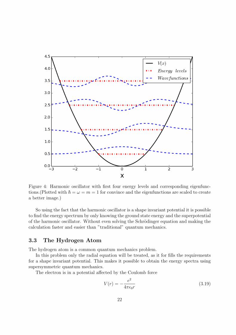
Figure 4: Harmonic oscillator with first four energy levels and corresponding eigenfunc-tions.(Plotted with ~ = ω = m = 1 for convince and the eigenfunctions are scaled to createa better image.)

So using the fact that the harmonic oscillator is a shape invariant potential it is possibleto find the energy spectrum by only knowing the ground state energy and the superpotentialof the harmonic oscillator. Without even solving the Schrodinger equation and making thecalculation faster and easier than ”traditional” quantum mechanics.

3.3 The Hydrogen Atom

The hydrogen atom is a common quantum mechanics problem.In this problem only the radial equation will be treated, as it for fills the requirements

for a shape invariant potential. This makes it possible to obtain the energy spectra usingsupersymmetric quantum mechanics.

The electron is in a potential affected by the Coulomb force

V (r) = − e2

4πε0r(3.19)

22

and the radial Schrodinger equation is

− ~2

2m

d2u

dr2+

[V (r) +

~2

2m

l(l + 1)

r2

]u(r) = Eu(r). (3.20)

The effective potential can be seen in fig.5

Figure 5: Radial coulomb potential (l = 1, e2

4πε0= 2, ~2

2m= 1)

In order to use supersymmetry, the ground state energy needs to be zero. So the shiftingpotential gives

Veff (r) = − e2

4πε0

1

r+

[~2l(l + 1)

2m

]1

r2− E0. (3.21)

The superpotential can be found by solving the differential equation given by Veff (r) =W (r)2 − ~√

2mW ′(r). Making the ansatz that the super potential will have the form

W (r) = B − C

r(3.22)

and inserting it into the differential equation gives

Veff (r) = B2 − 2BC

r+

[C2 − ~√

2mC

]1

r2. (3.23)

23

By comparing the Veff (r) in eq. (3.21) and Veff (r) in eq. (3.23) given by the differentialequation, makes it is possible to identify E0 = −B2 given the fact that B2 is the only termindependent of r. The other terms are identified as

2BC =e2

4πε0(3.24)

C2 − ~√2m

C =~2l(l + 1)

2m(3.25)

Solving these two equation, keeping in mind that we are looking for a positive l gives

C =~√2m

(l + 1) (3.26)

B =

√2m

~e2

8πε0(l + 1)(3.27)

Using the obtained constants B and C in the anzats gives the superpotential

W (r) =

√2m

~e2

8πε0(l + 1)− ~√

2m(l + 1)

1

r(3.28)

Using eq. (2.15) gives the partner potential

V (2)(r) =

(− e2

4πε0

)1

r+

(~2(l + 1)(l + 2)

2m

)1

r2+

(e4m

32π2~2ε20(l + 1)2

), (3.29)

it is shown in fig.6

24

Figure 6: Shifted potential and partner potential(l = 1, plotted with e2

4πε0= 2, ~2

2m= 1)

From the obtained value for B and the relation E0 = −B2 makes it possible to calculatethe ground state energy for hydrogen were l = 0,

E0 = −B2 = −

[√2m

~e2

8πε0

]2≈ −13.6eV. (3.30)

Looking at the shape invariant potential condition a2 = f(a1), by comparing the twopartner potentials Veff (r) and V (2)(r) it is possible to identify the relationship between theparameters

f(l) = l + 1 (3.31)

From this it is possible to find the remainder, R(l), that can be used to find the energydifference between the ground states for the two potentials.

(e4m

32π2~2ε20(l + 1)2

)=

(e4m

32π2~2ε20(l + 2)2

)+R(l)

⇒ R(l) =

(e4m(2l + 3)

32π2~2ε20(l + 1)2(l + 2)2

). (3.32)

25

To find the first excited state for the original problem, the energies need to be shiftedby the ground state

E1 = − e2m

32π~ε0(l + 1)2+

e4m(2l + 3)

32π2~2ε20(l + 1)2(l + 2)2, (3.33)

where n is the principal quantum number. Using the remainder eq. (3.32) and therelation for the parameter eq. (3.31) it is possible to obtain a formula the whole energyspectrum.

En = E0 +n∑i=1

e4(2(l + i− 1) + 3)

32π2~2ε20(l + i)2(l + i+ 1)2)2(3.34)

For the case l = 0 it is possible to rewrite the sum to

En =e4m

32π2~2ε20(n+ 1)2, (3.35)

which is the known formula for the energy levels of the hydrogen atom that can be seen infig.7.

Figure 7: Energy spectrum for the hydrogen atom (l = 0)

26

SUSYQM once again proved useful in providing an easier and faster solution to theproblem, and showing how useful it can be applied to more complex problem.

3.4 Relativistic Hydrogen Atom

The Schrodinger equation does not take in to account special relativity, in order to do soone has to use the Dirac equation. Using the Dirac equation to obtain the energy spectrumfor hydrogen, one gets a slightly different spectrum with splitting of energy levels. Thisis due to the fact that the Dirac equation takes into account relativistic and spin effectswhich leads to breaking of degeneracy for the energy levels.

For a central field potential it is possible to write the Dirac equation(~ = c = 1) [3] as

Hψ = (~α · ~p+ βm+ V )ψ (3.36)

where

αi =

(0 σi

σi 0

), β =

(1 00 −1

),1 =

(1 00 1

), V = −e

2

r(3.37)

σi are the Pauli spin matrices. In the case of the central field, the Dirac equation can beseparated into spherical coordinates. For the hydrogen atom is only required to use theradial part to calculate the energy spectra.

In order obtain the radial functions G and F for hydrogen the Dirac equation has thebe rewritten as a pair of first order equations [2].(

− d

dρ+τ

ρ

)F =

(−ν +

γ

ρ

)G (3.38)

(d

dρ+τ

ρ

)G =

(1

ν+γ

ρ

)F (3.39)

γ = Ze2 , k =√m2 − E2 , ρ = kr ,

ν =

√m− Em+ E

, τ =

[j +

1

2

]ω (3.40)

where j = l±±12,ω = ±1 for states of parity (−1)j+1/2 . It is possible to rewrite eq. (3.38)

and (3.39) in a more compact form(dG/drdF/dr

)+

1

r

(k −γγ −k

)(G)F

)=

((m+ E)G(m− E)F

)(3.41)

27

The matrix that is multiplied by 1r

mixes G and F . Needs to be diagonalized in orderto be rewritten in SUSYQM form. This is done by a linear transformation of the functionsG,F into G, F

D =

(k + s −γ−γ k + s

), s =

√k2 − γ2 (3.42)

(G

F

)= D

(GF

)(3.43)

and the supersymmetric form for the coupled equations

AF =

(m

E− k

s

)G , A†G = −

(m

E+k

s

)F (3.44)

where

A =d

dµ− s

µ+γ

s, A† = − d

dµ− s

µ+γ

s(3.45)

with the introduction of the variable µ = Er.Decoupling the equations for F and G gives the eigenvalue equations for F and G

H(1)F = A†AF =

(k2

s2− m2

E2

)F , (3.46)

H(2)G = AA†G =

(k2

s2− m2

E2

)G. (3.47)

Note that the two Hamiltonians eq. (3.46) and (3.47) are SUSYQM partner systems. Thetwo Hamiltonians are also shape invariant super symmetric partners due to fact that theycan be written on the form of a shape invariant potential, eq. (2.42)

H(2)(ρ, s, γ) = H(1)(ρ, s+ 1, γ) +γ2

s2− γ2

(s+ 1)2. (3.48)

Looking at the Shape Invariance condition gives

a2 = s+ 1 , a1 = s , R(a1) =γ2

a21− γ2

(a1 + 1)2(3.49)

so the energy spectra for H(1) are given by

E(1)n = E

(2)n−1 =

(k

s

)2

−(m2

E2n

)=

n∑k=1

R(ak) = γ2(

1

s2− 1

(s+ n)2

). (3.50)

28

Note that the H(1,2) is not the Dirac Hamiltonian with the sought after energy spectra. Itis possible to get the energy spectrum(En) for the hydrogen by relating it to E

(1)n through

eq. (3.46), eq. (3.47) and eq. (3.50).

En =m√

1 + γ2

(s+n)2

, n = 0, 1, 2... . (3.51)

Reintroducing ~ and c and setting Z = 1 in order to do calculations for hydrogen givesγ = α = e2

~c , using this in eq. (3.51)

Enj = m

1 +

α

n− (j + 12

+√

(j + 12)2 − α2

2−12

, n = 0, 1, 2... (3.52)

In fig.8 one can see the energy spectra and the non degeneracy caused by the quantumnumber l and in fig.9 is a comparison between the energy spectra for the relativistic andnon relativistic hydrogen atom.

Figure 8: Energy spectra for relativistic hydrogen atom. The splitting of energy levels isso small that it can’t be seen in the plot.

29

Figure 9: Comparison between the energy spectra for the relativistic and non relativistichydrogen atom. (Spectrum is scaled and shifted to create a better fig.)

Thus we proved that even the Dirac equation can be solved using the SUSYQM frame-work.

3.5 Isospectral Deformation of the Finite Square Well

Application of isospectral deformation to the finite square well, we are assuming that~√2m

= 1.The finite square well has the potential.

V0(x) =

{0, − L/2 ≤ x ≤ L/2V, otherwise

. (3.53)

The finite square well is a well known problem and the solution for the ground sate wavefunction and the ground state energy can be found several introductory book to quantummechanics [4].

The groundstate wavefunction is given by for each region of the potential

ψ0(x) =

Aeαx, x < L/2B cos(kx), −L/2 ≤ x ≤ L/2Ce−αx, x > L/2

. (3.54)

where the groundstate wavefunction is continuous. Using eq. (2.91) where I(x) =∫ x−∞[ψ

(1)0 (t)]2dt

to find the isospectral deformation of the potential, so by studying I(x) in region I,

30

x ∈ (−∞,−L/2) gives

II(x) =

∫ x

−∞[ψ0(t)]

2dt =

∫ x

−∞[Aeαx]2dt =

A2

2αe2αx (3.55)

and studying the isospectral deformation of the potential in the same region gives

VI(x) = VI − 2d2

dx2ln[II(x) + λ] = V − 16α32A2e2αxλ

(A2e2αx + 2αλ)2(3.56)

In region II, x ∈ [−L/2, L/2] gives

III(x) =

∫ x

−∞[ψ0(t)]

2dt =

∫ x

−L/2[Bcos(kt)]2dt+ II (−L/2)

=B2(sin(2kx) + 2kx+ sin(kL) + kL)

4k+ II (−L/2)

(3.57)

with the isospectral deformation of the potential

VII(x) = VII − 2d2

dx2ln[III(x) + λ] (3.58)

=8B2k2(2B2 cos(2kx) + (2B2kx+ 4kλ+B2(sin(kL) + kL) + 4II(−L/2)k) sin(2kx) + 2B2)

(B2 sin(2kx) + 2B2kx+ 4kλ+B2(sin(kL) + kL) + 4II(−L/2)k)2

(3.59)

In region III, x ∈ (L/2,∞)

I(x)III =

∫ x

−∞[ψ0(t)]

2dt =

∫ x

L/2

[Ce−αt]2dt+ III (L/2)

=1

2αC2(e2αx − eαL)e−2αx−αL + III (L/2) (3.60)

and studying in isospectral deformation of the potential in the same region gives

VIII(x) = VIII − 2d2

dx2ln[IIII(x) + λ]

= V +8α2C2e2αx+αL(2αeαLλ+ 2αeαLIII(L/2) + C2)

((e2αx(2αeαLλ+ 2αeαLIII(L/2) + C2) + C2)− C2eαL)2(3.61)

The isospectral deformation of the finite square well for a few lambdas is plotted infig.10.

31

Figure 10: Isospectral deformation of finite square well, plotted with ~√2m

= 1, V = 20 andL = π.

3.6 Isospectral Deformation from a Wave Function

It is possible to construct a potential from just knowing the ground state wave function,assuming it for fills the SUSYQM requirements i.e. it needs to be nodeless. Using eq. (2.3)and the assumption ~2

2m= 1.

V (1)(x) =ψ′′0(x)

ψ0(x). (3.62)

So doing this with the wave function

ψ0(x) = A(1 + βx2)e−αx2

, (3.63)

where A is the normalization constant, note that it is nodeless for β ≥ 0.

V (x) =ψ′′0(x)

ψ0(x)=

(4α2βx4 + 2α(2α− 5β)x2 − 2(α− β))

(1 + βx2)(3.64)

32

So from this it is possible to construct an isospectral deformation of the potential usingeq. (2.91) where I(x) =

∫ x−∞[ψ0(t)]

2dt, so by studying I(x) and using the gamma function,Γ(s) and the incomplete gamma function, γ(s, t) were

γ(s, t) =

∫ x

0

ts−1e−tdt, Γ(s) =

∫ ∞0

ts−1e−tdt (3.65)

to rewrite it, gives

I(x) =

∫ x

−∞[A(1 + βt2)e−αt

2

]2dt

= A2

∫ x

−∞e−2αt

2

dt+ A2

∫ x

−∞2βt2e−2αt

2

dt+ A2

∫ x

−∞β2t4e−2αt

2

dt

=A2

√8α

∫ 2αx2

−∞

1√ze−zdz +

2A2β√8α3

∫ 2αx2

−∞

√ze−zdz +

A2β2

√32α5/2

∫ 2αx2

−∞z3/2e−zdz

At this point it is easy to normalize the wave function simply by introducing thenormalization condition by changing the integration region for I(x) i.e.∫ ∞

−∞[A(1 + βt2)e−αt

2

]2dt = 1

= A2

∫ ∞−∞

e−2αt2

dt+ A2

∫ ∞−∞

2βt2e−2αt2

dt+ A2

∫ ∞−∞

β2t4e−2αt2

dt = 1

=2A2

√8α

Γ(1

2) +

2A2β√8α3

Γ(3

2) +

A2β2

√32α5/2

Γ(5

2) = 1

=⇒ A =

(2√8α

√π +

β√8α3

√π +

3

4

β2

√32α5/2

√π

)− 12

(3.66)

Getting back to I(x)

I(x) =A2

√8α

(√π ± γ

(1

2, 2αx2

))+

A2β√8α3

(1

2

√π ± γ

(3

2, 2αx2

))

+

√2A2β2

16α5/2

(3

4

√π ± γ

(5

2, 2αx2

)),

{+, x > 0−, x < 0

. (3.67)

33

and the isospectral deformation of the potential is given by

V (x) = V (x)− 2d2

dx2ln[I(x) + λ] = V (x)− 2

(I(x) + λ)I ′′(x)− I ′(x)I ′(x)

(I(x) + λ)2(3.68)

where

I ′(x) = [ψ0(x)]2 =[A(1 + βx2)e−αx

2]2, (3.69)

I ′′(x) = (4β2A2x3 − 4αβ2A2x5)e−2αx2

(3.70)

In fig.11 the potential is plotted for some different lambdas and in fig. 12 the corre-sponding wave functions are plotted using eq. (2.92), with α = 1/2 and β = 2.

Figure 11: Isospectral deformation of the potential created with the wave function eq.(3.63), plotted with ~2

2m= 1, α = 1/2 and β = 2 (arb. units).

34

Figure 12: Wave functions corresponding to the isospectral deformation of the potentialcreated with the wave function eq. (3.63), plotted with ~2

2m= 1, α = 1/2 and β = 2 (arb.

units).

4 Conclusions

Supersymmetric quantum mechanics provides a different approach to solving a number ofquantum mechanical problems. Using SUSYQM and the shape invariant condition it ispossible to calculate the energy spectra without solving the Schrodinger equation or theDirac equation, by finding the superpotential and using it to generate partner potentials.Were the partner potentials has the same energy spectra except for the ground state.

Supersymmetric quantum mechanics provides a new aspect to quantum mechanics.Shows the difficulty of the inverse problem, instead of asking “For a given potential, whatare the allowed energies it produces?” one could ask “For a given set of energylevels energy,what are the potentials that could have produced it?” [1].

The fact that seemingly unrelated potentials have almost identical energy spectra iscaused by the fact that they have the same underlying superpotential or are a part ofthe same isospectral deformation family. This is not explained in traditional quantummechanics and are one of the oddities in traditional quantum mechanics. Thus it providesa deeper understanding of a quantum mechanics.

Supersymmetric quantum mechanics can be applied to a wide range of quantum me-chanics problems, such as obtaining the energy spectra for a hydrogen atom as well asobtaining the fine structure for the energy spectrum of the hydrogen atom from the Diracequation without solving it explicitly.

35

References

[1] Constantin Rasinariu Asim Gangopadhyaya, Jeffry V Mallow. SuperSymmetric Quan-tum Mechanics. World Scientific, 2011.

[2] H. Bethe and E.E. Salpeter. Quantum Mechanics of One- and Two- Electron Atoms.Springer, 1977.

[3] Fred Cooper, Avinash Khare, and Uday Sukhatme. Supersymmetry and quantummechanics. Phys.Rept., 251:267–385, 1995.

[4] David J Grittiths. Introduction to quantum mechanics. Pearson Prentice Hall, 2005.

[5] Richard L. Liboff. Introductory Quantum Mechanics. Addison-Wesley, 2002.

[6] Jens Maluck. Bachelor thesis: An introduction to supersymmetric quantum mechanicsand shape invariant potentials, 2013.

[7] Edward Witten. Dynamical Breaking of Supersymmetry. Nucl.Phys., B188:513, 1981.

36