Summer School on Multidimensional

Poverty Analysis

3–15 August 2015

Georgetown University, Washington, DC, USA

Multidimensional Poverty Measurement

Methodologies and Counting Approaches

Sabina Alkire, George Washington University & OPHI

Suman Seth, University of Leeds and OPHI

Paola Ballon, OPHI

Session II, 4 August 2015

Bring diverse methodologies into common framework

Clarify each methodology, data requirements, assumptions,

and key choices in measurement design

Evaluate pros and cons of each approach

Enable readers to make informed choices about which

approach best addresses a given problem

Aim of this Session

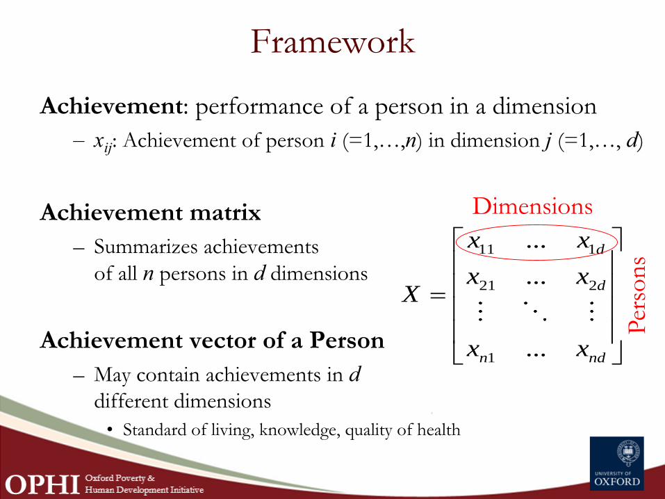
Achievement: performance of a person in a dimension

– xij: Achievement of person i (=1,…,n) in dimension j (=1,…, d)

Achievement matrix

– Summarizes achievements

of all n persons in d dimensions

Achievement vector of a Person

– May contain achievements in d

different dimensions

• Standard of living, knowledge, quality of health

11 1

21 2

1

...

...

...

d

d

n nd

x x

x xX

x x

Dimensions

Per

son

s

Framework

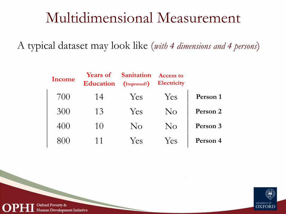
A typical dataset may look like (with 4 dimensions and 4 persons)

IncomeYears of

Education

Sanitation

(Improved?)

Access to

Electricity

700 14 Yes Yes Person 1

300 13 Yes No Person 2

400 10 No No Person 3

800 11 Yes Yes Person 4

Multidimensional Measurement

Framework

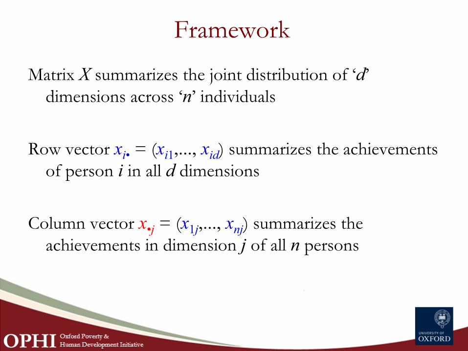
Matrix X summarizes the joint distribution of ‘d’

dimensions across ‘n’ individuals

Row vector xi• = (xi1,..., xid) summarizes the achievements

of person i in all d dimensions

Column vector x•j = (x1j,..., xnj) summarizes the

achievements in dimension j of all n persons

Measurement of multidimensional poverty generally involves

three major steps

– Choice of space: How should we define poverty?

– Identification: Who is poor?

– Aggregation: How should the information of all the poor

be aggregated to obtain an index?

Multidimensional Measurement

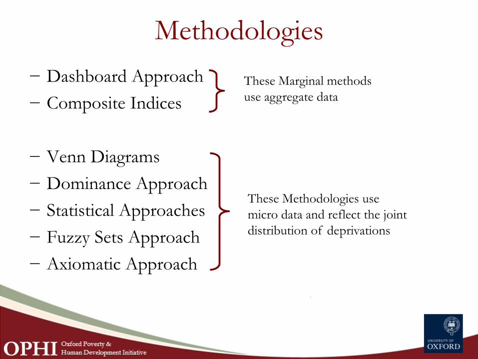
Methodologies

− Dashboard Approach

− Composite Indices

− Venn Diagrams

− Dominance Approach

− Statistical Approaches

− Fuzzy Sets Approach

− Axiomatic Approach

These Marginal methods

use aggregate data

These Methodologies use

micro data and reflect the joint

distribution of deprivations

Dashboard Approach

A set of dimensions (indicators), which applies “a

unidimensional measure to each dimension” (Alkire, Foster, Santos, 2011)

Applications

– Basic Needs Approach

• As a first step, it might be useful to define the best indicator for each

basic need...” (Hicks & Streeten, 1979)

– Millennium Development Goals (UN, 2000)

Examples: Percent of malnourished children, Infant

Mortality Rate, Illiteracy rate

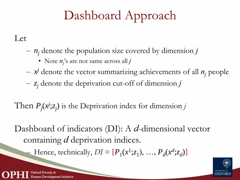
Dashboard Approach

Let

– nj denote the population size covered by dimension j

• Note nj’s are not same across all j

– xj denote the vector summarizing achievements of all nj people

– zj denote the deprivation cut-off of dimension j

Then Pj(xj;zj) is the Deprivation index for dimension j

Dashboard of indicators (DI): A d-dimensional vector

containing d deprivation indices.

– Hence, technically, DI = [P1(x1;z1), …, Pd(x

d;zd)]

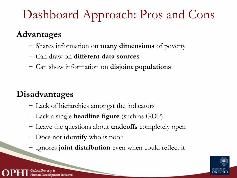
Dashboard Approach: Pros and Cons

Advantages

− Shares information on many dimensions of poverty

− Can draw on different data sources

− Can show information on disjoint populations

Disadvantages

− Lack of hierarchies amongst the indicators

− Lack a single headline figure (such as GDP)

− Leave the questions about tradeoffs completely open

− Does not identify who is poor

− Ignores joint distribution even when could reflect it

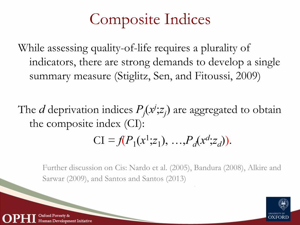
Composite Indices

While assessing quality-of-life requires a plurality of

indicators, there are strong demands to develop a single

summary measure (Stiglitz, Sen, and Fitoussi, 2009)

The d deprivation indices Pj(xj;zj) are aggregated to obtain

the composite index (CI):

CI = f(P1(x1;z1), …,Pd(x

d;zd)).

Further discussion on Cis: Nardo et al. (2005), Bandura (2008), Alkire and

Sarwar (2009), and Santos and Santos (2013)

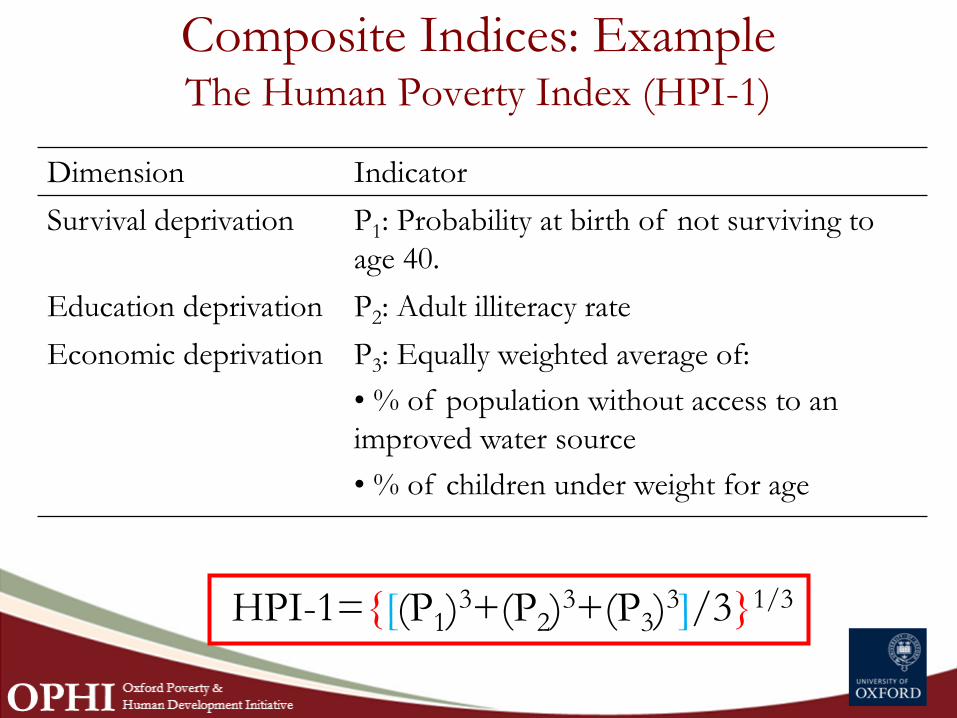
Composite Indices: ExampleThe Human Poverty Index (HPI-1)

Dimension Indicator

Survival deprivation P1: Probability at birth of not surviving to

age 40.

Education deprivation P2: Adult illiteracy rate

Economic deprivation P3: Equally weighted average of:

• % of population without access to an

improved water source

• % of children under weight for age

HPI-1={[(P1)3+(P2)

3+(P3)3]/3}1/3

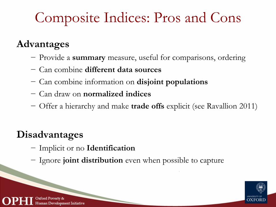
Composite Indices: Pros and Cons

Advantages

− Provide a summary measure, useful for comparisons, ordering

− Can combine different data sources

− Can combine information on disjoint populations

− Can draw on normalized indices

− Offer a hierarchy and make trade offs explicit (see Ravallion 2011)

Disadvantages

− Implicit or no Identification

− Ignore joint distribution even when possible to capture

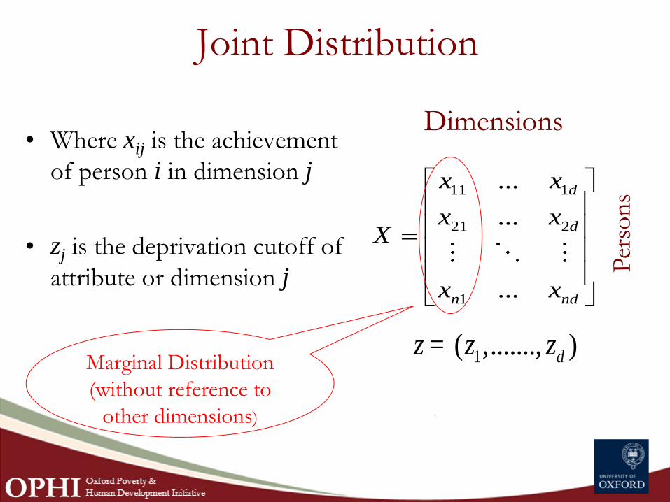
Joint Distribution

• Where xij is the achievement

of person i in dimension j

• zj is the deprivation cutoff of

attribute or dimension j

1( ,......., )= dz z z

Dimensions

Per

son

s11 1

21 2

1

...

...

...

d

d

n nd

x x

x xX

x x

Marginal Distribution

(without reference to

other dimensions)

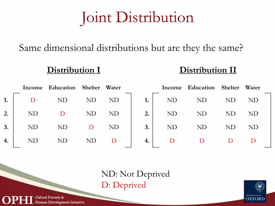
Joint Distribution

Income Education Shelter Water

1. D ND ND ND

2. ND D ND ND

3. ND ND D ND

4. ND ND ND D

Income Education Shelter Water

1. ND ND ND ND

2. ND ND ND ND

3. ND ND ND ND

4. D D D D

Distribution I Distribution II

ND: Not Deprived

D: Deprived

Same dimensional distributions but are they the same?

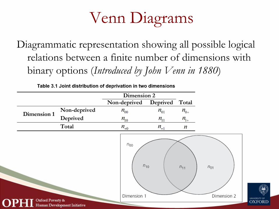
Venn Diagrams

Diagrammatic representation showing all possible logical

relations between a finite number of dimensions with

binary options (Introduced by John Venn in 1880)

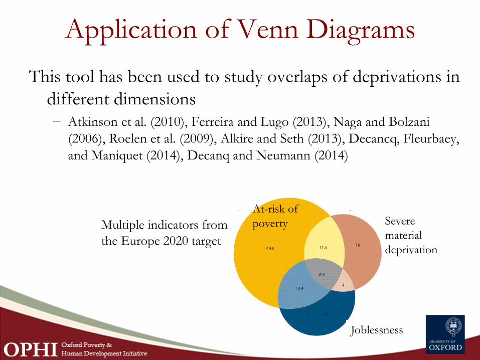
Application of Venn Diagrams

Multiple indicators from

the Europe 2020 target

At-risk of

poverty Severe

material

deprivation

Joblessness

This tool has been used to study overlaps of deprivations in

different dimensions

− Atkinson et al. (2010), Ferreira and Lugo (2013), Naga and Bolzani

(2006), Roelen et al. (2009), Alkire and Seth (2013), Decancq, Fleurbaey,

and Maniquet (2014), Decanq and Neumann (2014)

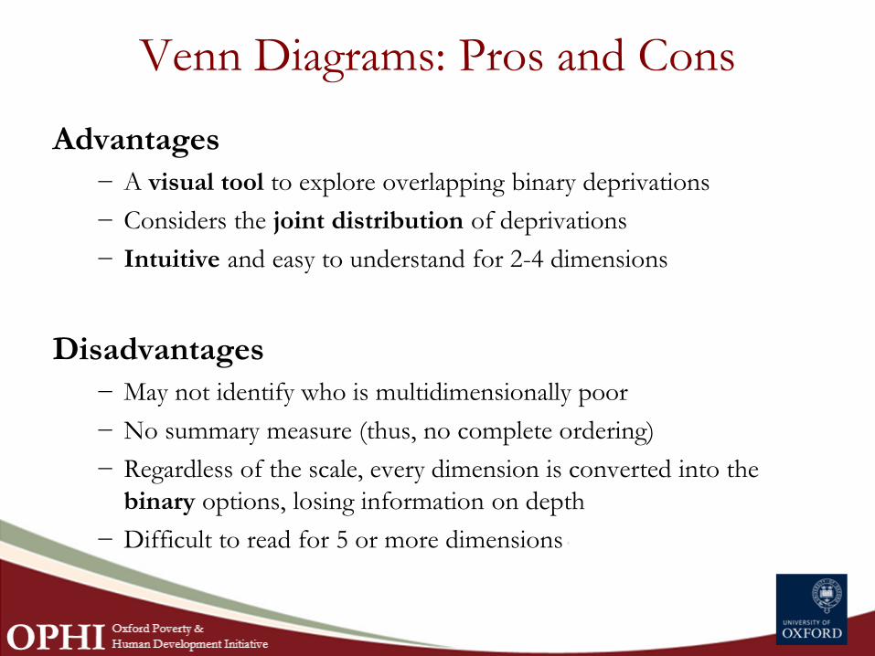
Venn Diagrams: Pros and Cons

Advantages

− A visual tool to explore overlapping binary deprivations

− Considers the joint distribution of deprivations

− Intuitive and easy to understand for 2-4 dimensions

Disadvantages

− May not identify who is multidimensionally poor

− No summary measure (thus, no complete ordering)

− Regardless of the scale, every dimension is converted into the

binary options, losing information on depth

− Difficult to read for 5 or more dimensions

Dominance Approach

Ascertains whether poverty is unambiguously lower or

higher regardless of parameters and poverty measures

− Unidimensional: Atkinson (1987), Foster and Shorrocks (1988)

− Multidimensional: Bourguignon and Chakravarty (2002), Duclos,

Sahn & Younger (2006)

Such a claim certainly has strong political power!

– Avoids the possibility of contradictory rankings

Key tool: Cumulative distribution function

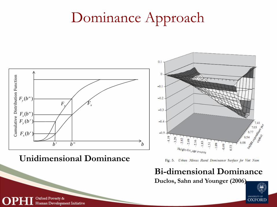
Dominance Approach

Unidimensional Dominance

Bi-dimensional DominanceDuclos, Sahn and Younger (2006)

b ' b '' b

Cu

mu

lati

ve

Dis

trib

uti

on

Fu

nct

ion

yF xF( )yF b"

( )xF b"

( )yF b'

( )xF b'

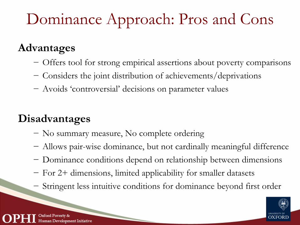
Dominance Approach: Pros and Cons

Advantages

− Offers tool for strong empirical assertions about poverty comparisons

− Considers the joint distribution of achievements/deprivations

− Avoids ‘controversial’ decisions on parameter values

Disadvantages

− No summary measure, No complete ordering

− Allows pair-wise dominance, but not cardinally meaningful difference

− Dominance conditions depend on relationship between dimensions

− For 2+ dimensions, limited applicability for smaller datasets

− Stringent less intuitive conditions for dominance beyond first order

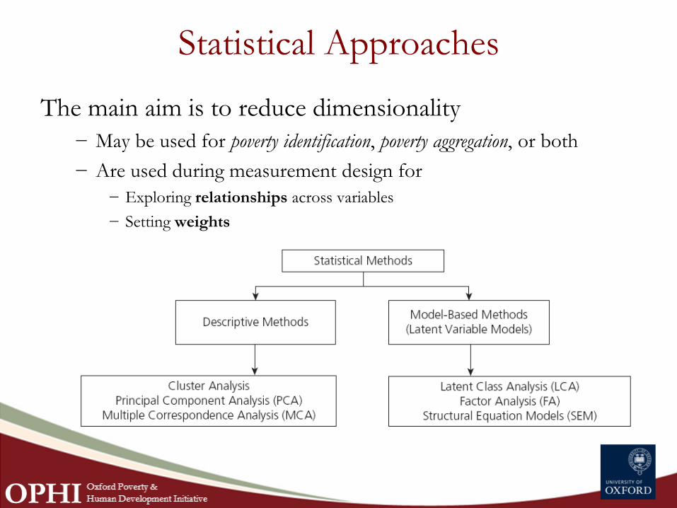
Statistical Approaches

The main aim is to reduce dimensionality

− May be used for poverty identification, poverty aggregation, or both

− Are used during measurement design for

− Exploring relationships across variables

− Setting weights

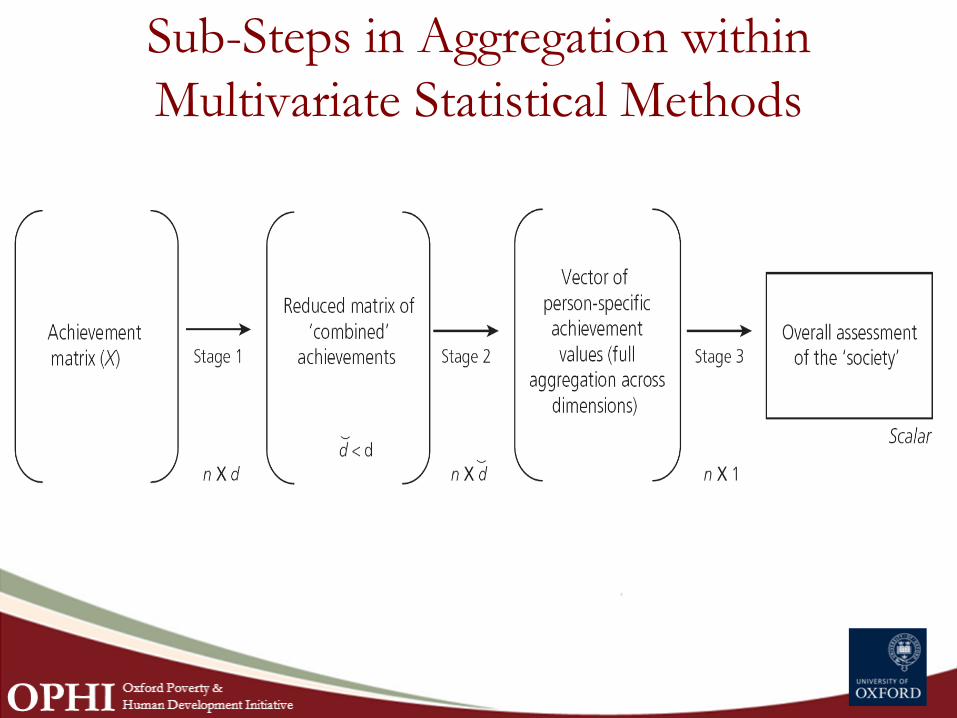
Sub-Steps in Aggregation within

Multivariate Statistical Methods

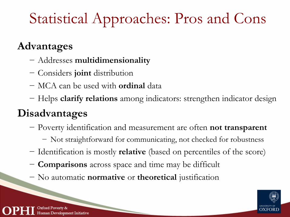
Statistical Approaches: Pros and Cons

Advantages

− Addresses multidimensionality

− Considers joint distribution

− MCA can be used with ordinal data

− Helps clarify relations among indicators: strengthen indicator design

Disadvantages

− Poverty identification and measurement are often not transparent

− Not straightforward for communicating, not checked for robustness

− Identification is mostly relative (based on percentiles of the score)

− Comparisons across space and time may be difficult

− No automatic normative or theoretical justification

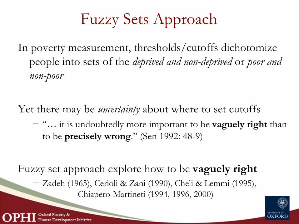
Fuzzy Sets Approach

In poverty measurement, thresholds/cutoffs dichotomize

people into sets of the deprived and non-deprived or poor and

non-poor

Yet there may be uncertainty about where to set cutoffs

− “… it is undoubtedly more important to be vaguely right than

to be precisely wrong.” (Sen 1992: 48-9)

Fuzzy set approach explore how to be vaguely right

− Zadeh (1965), Cerioli & Zani (1990), Cheli & Lemmi (1995),

Chiapero-Martineti (1994, 1996, 2000)

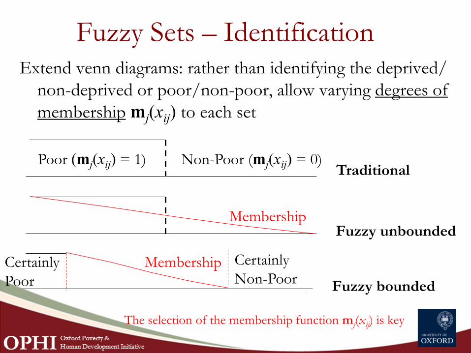
Fuzzy Sets – IdentificationExtend venn diagrams: rather than identifying the deprived/

non-deprived or poor/non-poor, allow varying degrees of

membershipmj(xij) to each set

The selection of the membership function mj(xij) is key

Poor (mj(xij) = 1) Non-Poor (mj(xij) = 0)Traditional

Fuzzy unboundedMembership

Fuzzy bounded

MembershipCertainly

Poor

Certainly

Non-Poor

Fuzzy Sets Approach: Pros and Cons

Advantages

− Offers summary measure, hierarchy among dimensions, explicit

tradeoffs and a complete ranking

− Can consider joint distribution of deprivations

− Compatible with many aggregation methodologies (Chakravarty 2006)

Disadvantages

− Justification of membership function is not straightforward

− Robustness tests are not mostly provided

− Some membership functions may misuse ordinal data

− Fuzzy sets results may conflict with Dominance results

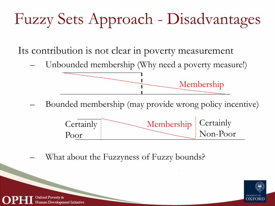
Fuzzy Sets Approach - Disadvantages

Its contribution is not clear in poverty measurement

– Unbounded membership (Why need a poverty measure!)

– Bounded membership (may provide wrong policy incentive)

– What about the Fuzzyness of Fuzzy bounds?

Membership

MembershipCertainly

Poor

Certainly

Non-Poor

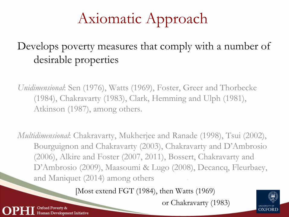
Axiomatic Approach

Develops poverty measures that comply with a number of

desirable properties

Unidimensional: Sen (1976), Watts (1969), Foster, Greer and Thorbecke

(1984), Chakravarty (1983), Clark, Hemming and Ulph (1981),

Atkinson (1987), among others.

Multidimensional: Chakravarty, Mukherjee and Ranade (1998), Tsui (2002),

Bourguignon and Chakravarty (2003), Chakravarty and D’Ambrosio

(2006), Alkire and Foster (2007, 2011), Bossert, Chakravarty and

D’Ambrosio (2009), Maasoumi & Lugo (2008), Decancq, Fleurbaey,

and Maniquet (2014) among others

[Most extend FGT (1984), then Watts (1969)

or Chakravarty (1983)

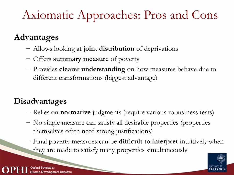
Advantages

− Allows looking at joint distribution of deprivations

− Offers summary measure of poverty

− Provides clearer understanding on how measures behave due to

different transformations (biggest advantage)

Disadvantages

− Relies on normative judgments (require various robustness tests)

− No single measure can satisfy all desirable properties (properties

themselves often need strong justifications)

− Final poverty measures can be difficult to interpret intuitively when

they are made to satisfy many properties simultaneously

Axiomatic Approaches: Pros and Cons

Counting Approach:

History

Counting Approach

Refers to a particular method for identifying the poor

− Entails ‘counting the number of dimensions in which people

suffer deprivation, (…) the number of dimensions in which

they fall below the threshold’. Atkinson (2003: 51)

Associated to the ‘direct method’ to measure poverty

(Sen, 1981)

Widely used in practice and policy since mid 1970s

Counting Approach

Steps for identifying a poor person

1. Define a list of relevant indicators

2. Assign a weight to each considered indicator

3. Define a threshold (deprivation cutoff) for each indicator

4. Create binary deprivation scores for each person in each

indicator: “1” = deprived, “0” = non-deprived

5. Produce a deprivation score by taking a weighted sum of

deprivations

6. Set a threshold (or poverty cutoff) such that if a person has a

deprivation score at or above the threshold, the person is

considered poor

Counting Approach

The approach has been applied within different conceptual

frameworks:

− Social Exclusion in Europe (Lenoir, 1974)

− Basic Needs in Latin America (Cocoyoc Declaration, 1974)

− More recently: capability approach, human rights approach

Applications in different parts of the world

− Europe, US, Latin America, South Asia

− UNICEF, NGOs (BRAC)

Salient Implementations: Europe

Townsend (1979), “Poverty in the UK”

− Listed 60 indicators covering 12 dimensions

− Then focused on a shorter list of 12 items

− Equal weights to all indicators

− Used a minimum score of five ‘as suggestive of deprivation’

− But, used this approach only to ‘validate’ the income poverty

line to be for poverty measurement

Townsend’s work inspired a prominent body of subsequent work

within and outside Europe

Salient Implementations: Europe

Mack and Lansley (1985), “Poor Britain” (2 innovations)

− Socially perceived necessities (Breadline Britain survey)

− Retained 26 items considered necessary by more than 50% of

population (majority rule)

− Enforced lack

− Distinguished people not having an item as they could not

afford it, from those it was a voluntary choice

− How were the poor identified?

− Who could not afford three or more items

− Indicators were equally weighted

Callan, Nolan and Whelan (1993)

− Listed 8 items of the basic lifestyle dimension.

− Who were the poor?

− Those deprived in one or more of the eight items and below

the relative income poverty line (60% of average income)

− Consistent poverty approach (intersection of two approaches)

Salient Implementations: Europe

39

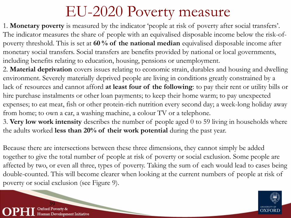
EU-2020 Poverty measure1. Monetary poverty is measured by the indicator ‘people at risk of poverty after social transfers’.

The indicator measures the share of people with an equivalised disposable income below the risk-of-

poverty threshold. This is set at 60 % of the national median equivalised disposable income after

monetary social transfers. Social transfers are benefits provided by national or local governments,

including benefits relating to education, housing, pensions or unemployment.

2. Material deprivation covers issues relating to economic strain, durables and housing and dwelling

environment. Severely materially deprived people are living in conditions greatly constrained by a

lack of resources and cannot afford at least four of the following: to pay their rent or utility bills or

hire purchase instalments or other loan payments; to keep their home warm; to pay unexpected

expenses; to eat meat, fish or other protein-rich nutrition every second day; a week-long holiday away

from home; to own a car, a washing machine, a colour TV or a telephone.

3. Very low work intensity describes the number of people aged 0 to 59 living in households where

the adults worked less than 20% of their work potential during the past year.

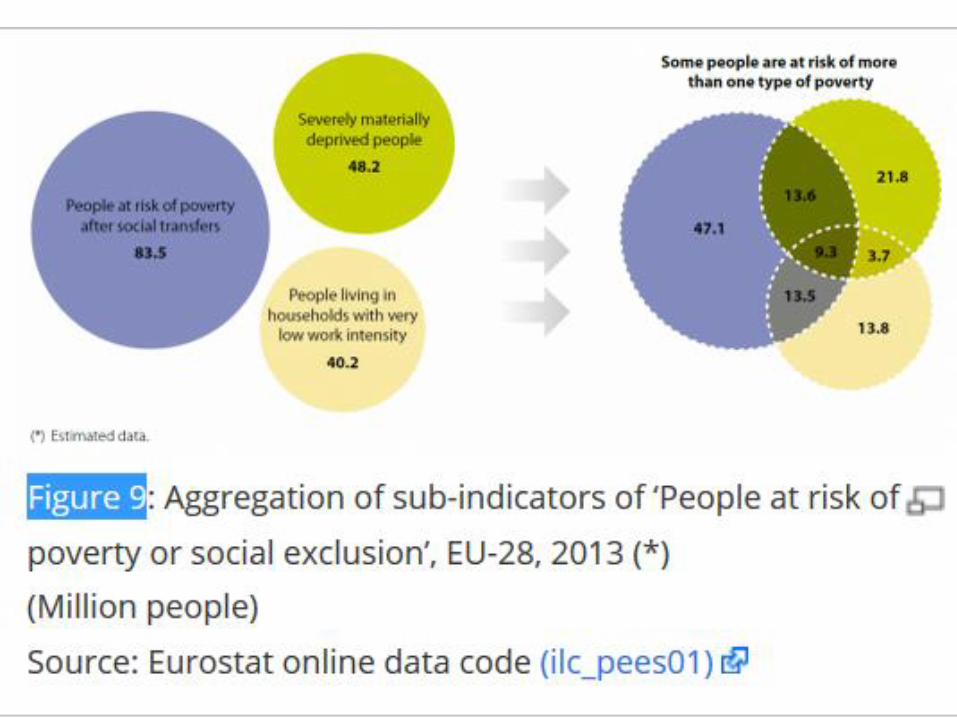
Because there are intersections between these three dimensions, they cannot simply be added

together to give the total number of people at risk of poverty or social exclusion. Some people are

affected by two, or even all three, types of poverty. Taking the sum of each would lead to cases being

double-counted. This will become clearer when looking at the current numbers of people at risk of

poverty or social exclusion (see Figure 9).

40

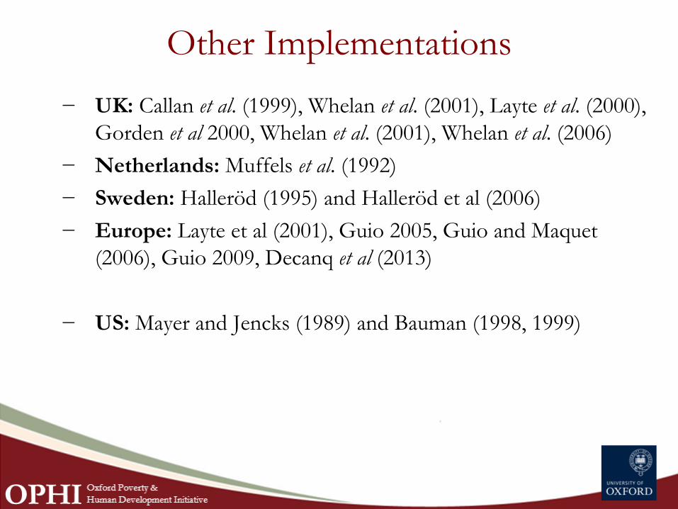
− UK: Callan et al. (1999), Whelan et al. (2001), Layte et al. (2000),

Gorden et al 2000, Whelan et al. (2001), Whelan et al. (2006)

− Netherlands: Muffels et al. (1992)

− Sweden: Halleröd (1995) and Halleröd et al (2006)

− Europe: Layte et al (2001), Guio 2005, Guio and Maquet

(2006), Guio 2009, Decanq et al (2013)

− US: Mayer and Jencks (1989) and Bauman (1998, 1999)

Other Implementations

− Unsatisfied Basic Needs (UBN) Approach

− Chile (Kast and Molina, 1975)

− Argentina (INDEC 1984, together with CEPAL)

− Used five census indicators– (i) Overcrowding, (ii) Housing, (iii) Sanitation, (iv) Children

attending primary school, (v) Household head has 2 or less

years of education, or high dependency rate

– Reported headcount ratio with 1+, 2+ and 3+ deprivations

– Used for policy mapping at very disaggregated levels

– Extensions: Bolivia, Colombia, Ecuador, Guatemala,

Honduras, Nicaragua, Paraguay, Peru, Uruguay, Venezuela

Salient Implementations: Latin America

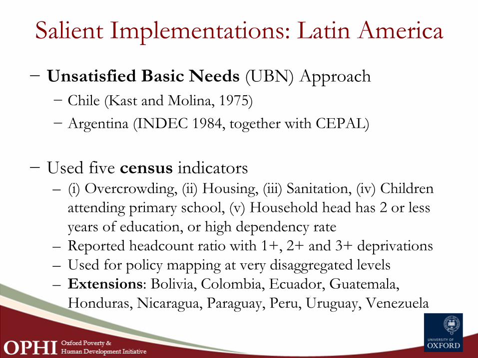
− Unsatisfied Basic Needs (UBN) Approach

− Chile (Kast and Molina, 1975)

− Argentina (INDEC 1984, together with CEPAL)

− Used five census indicators– (i) Overcrowding, (ii) Housing, (iii) Sanitation, (iv) Children

attending primary school, (v) Household head has 2 or less

years of education, or high dependency rate

– Reported headcount ratio with 1+, 2+ and 3+ deprivations

– Used for policy mapping at very disaggregated levels

– Extensions: Bolivia, Colombia, Ecuador, Guatemala,

Honduras, Nicaragua, Paraguay, Peru, Uruguay, Venezuela

Salient Implementations: Latin America

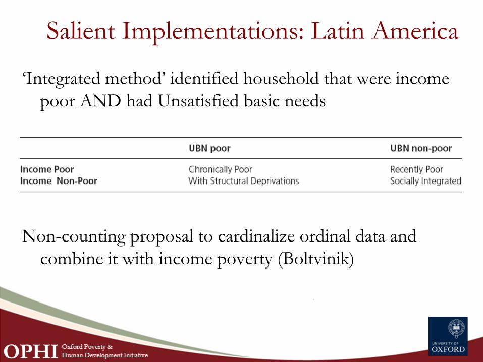
‘Integrated method’ identified household that were income

poor AND had Unsatisfied basic needs

Non-counting proposal to cardinalize ordinal data and

combine it with income poverty (Boltvinik)

Salient Implementations: Latin America

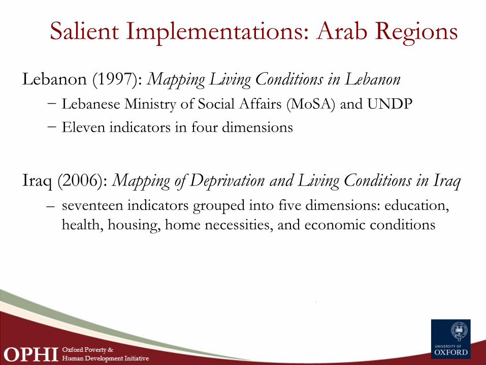
Lebanon (1997): Mapping Living Conditions in Lebanon

− Lebanese Ministry of Social Affairs (MoSA) and UNDP

− Eleven indicators in four dimensions

Iraq (2006): Mapping of Deprivation and Living Conditions in Iraq

– seventeen indicators grouped into five dimensions: education,

health, housing, home necessities, and economic conditions

Salient Implementations: Arab Regions

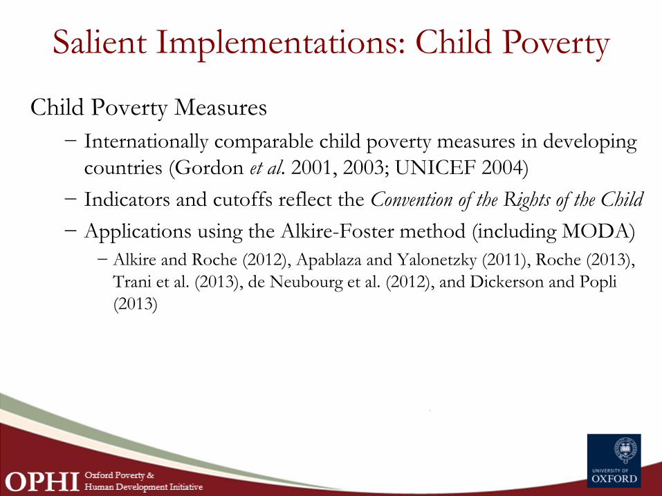
Child Poverty Measures

− Internationally comparable child poverty measures in developing

countries (Gordon et al. 2001, 2003; UNICEF 2004)

− Indicators and cutoffs reflect the Convention of the Rights of the Child

− Applications using the Alkire-Foster method (including MODA)

− Alkire and Roche (2012), Apablaza and Yalonetzky (2011), Roche (2013),

Trani et al. (2013), de Neubourg et al. (2012), and Dickerson and Popli

(2013)

Salient Implementations: Child Poverty

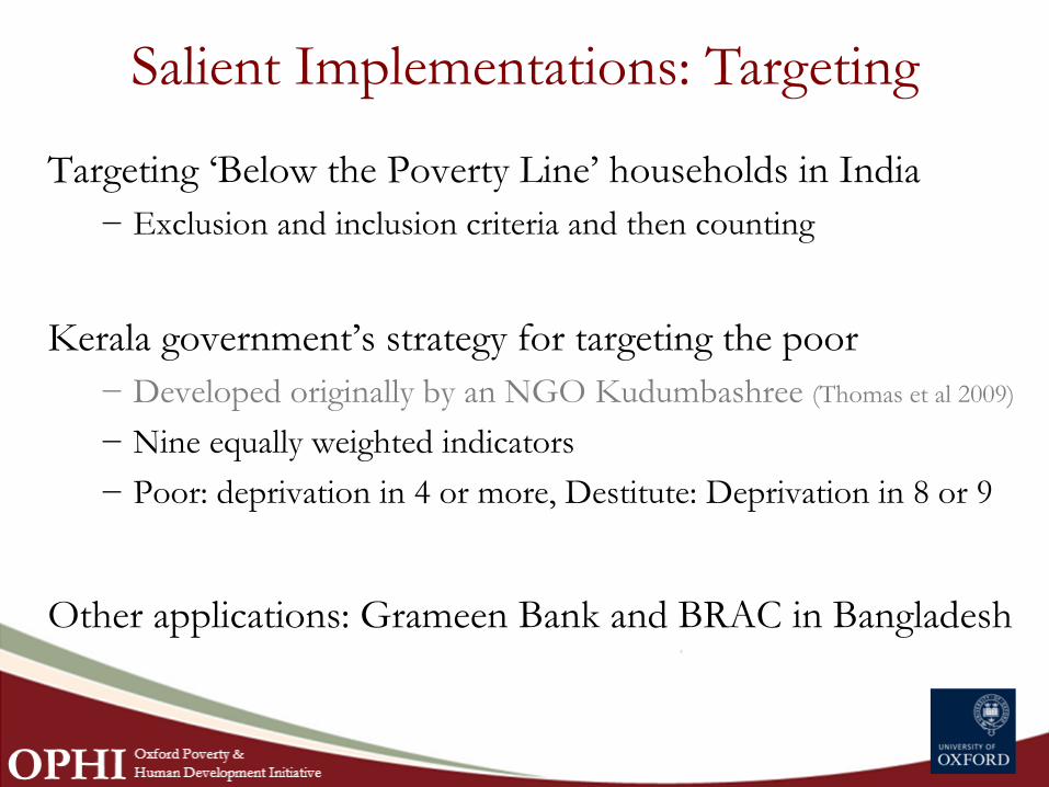
Targeting ‘Below the Poverty Line’ households in India

− Exclusion and inclusion criteria and then counting

Kerala government’s strategy for targeting the poor

− Developed originally by an NGO Kudumbashree (Thomas et al 2009)

− Nine equally weighted indicators

− Poor: deprivation in 4 or more, Destitute: Deprivation in 8 or 9

Other applications: Grameen Bank and BRAC in Bangladesh

Salient Implementations: Targeting

Advantages

− Clarity, Simplicity, Transparency, Intuition for identifying the

multiply deprived

− Allows looking at joint deprivations

− Allows for both cardinal and ordinal variables

Counting Approach: Pros and Cons

Disadvantages

− Relies on the particular selection of indicators (appropriateness for

the particular purpose)

− Relies on the weights assigned to the dimensions/indicators.

− Relies on dichotomies (deprived/non-deprived) so not sensitive to

the depth for identification.

− Sometimes a counting approach is combined with aggregation

methodologies that are not intuitive, in certain cases incorrectly

assigning cardinal meaning to ordinal values (ex. poverty scorecards)

Counting Approach: Pros and Cons