Studies of Transonic Cavity Flows - NATO Meeting Proceedings/RTO... · Cranfield University, RMCS Shrivenham ... School of Engineering, Cranfield University, Cranfield, ... Studies

RTO-MP-AVT-108 23 - 1

UNCLASSIFIED/UNLIMITED


Studies of Transonic Cavity Flows Relevant to Aircraft Stores Carriage and Release

K. Knowles, N .J. Lawson*, D. Bray, S.A. Ritchie and P. Geraldes Aeromechanical Systems Group

Cranfield University, RMCS Shrivenham Swindon, Wiltshire, SN6 8LA, UK

[email protected]

ABSTRACT

Particle image velocimetry (PIV) measurements are presented from rectangular cavities of different length-to-depth ratios at a Mach number of 0.85 in the RMCS transonic wind tunnel. The measurements are made in l/h=5 and l/h=14 cavities in order to encompass the open and closed flow regimes. The time- averaged two-dimensional PIV results are compared with time-averaged two-dimensional URANS CFD predictions. Streamwise and vertical velocity components are compared for three depths within the cavity; y/h=0.25, y/h=0.5 and y/h=0.75. Good agreement is found in the mean flow structure between the experimental and numerical data collected for the study. The maximum flow velocities extracted from the PIV data for the ‘open’ cavity case are generally lower than those predicted by the CFD model. The maximum flow velocities extracted from the ‘closed’ cavity PIV data are generally higher than the values predicted by the CFD model. Three-dimensional features of transonic cavity flows are discussed.

NOMENCLATURE

h cavity depth

l cavity length

M Mach number

N Number of samples

V local velocity magnitude

u streamwise velocity component

v vertical velocity component

w cavity width

x streamwise direction

y depthwise direction

z spanwise direction

Subscripts ∞ Freestream condition

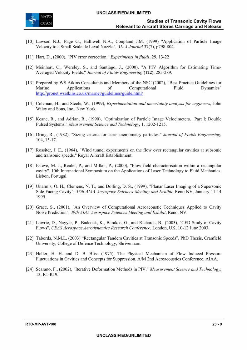
Cavity geometries are consistent with the standard ESDU cavity notation [1] as seen in Figure 1.

* Present address: School of Engineering, Cranfield University, Cranfield, Bedfordshire, MK43 0AL, UK.

Paper presented at the RTO AVT Symposium on “Functional and Mechanical Integration of Weapons and Land and Air Vehicles”, held in Williamsburg, VA, USA, 7-9 June 2004, and published in RTO-MP-AVT-108.


23 - 2 RTO-MP-AVT-108



1.0 INTRODUCTION

The advent of stealth aircraft, and the consequent requirement for aircraft designs with reduced radar signatures, has prompted the need for weapons to be stored internally in, and released from, bomb bays. Once the bomb bay doors are opened a cavity flow is produced. Cavity flows can be defined as one of two main types, primarily dependent on the length-to-depth ratio (L/D) of the cavity [2][3]. “Open” cavity flows occur in cavities with L/D<10 (Fig 2) and are characterised by strong pressure oscillations which lead to noise radiation (often in excess of 170dB), structural vibration and high levels of heat transfer at the trailing edge. “Closed” cavity flows occur in cavities with L/D>13 and are regarded as quasi-steady flows (Fig 3). The pressure distribution along the roof of a “closed” cavity shows a large longitudinal pressure gradient that causes a large increase in pressure drag and can lead to store separation difficulties. Cavity geometries in the range 10<L/D<13 are described as “transitional” and here the cavity flows exhibit a combination of “open” and “closed” flow features.

Many previous studies of cavity flows have concentrated on the time-averaged and unsteady measurement of the flow using static pressure taps on the surfaces and qualitative visualisation techniques like schlieren imagery and oil flow visualisation [4][5][6]. The results of these studies have typically been compared to numerical models with mixed success [7][8]. There is currently very little data available on the off-surface flowfield within different cavity geometries under transonic conditions. Advanced optical techniques such as particle image velocimetry (PIV) [9] now offer the potential to record quantitative velocity data from transonic and supersonic flows [10].

2.0 EXPERIMENTATION

2.1 Transonic Wind Tunnel All tests were conducted using the Royal Military College of Science (RMCS) transonic wind tunnel (TWT), a schematic of which is seen in Figure 4. The tunnel has a working section of 206mm (height) by 229mm (width). The facility is a closed circuit ejector driven tunnel supplied with air from two Howden screw-type compressors. The compressors supply air at up to 7 bar(g), which is dried and stored in a 34m³ reservoir. The stored air is sufficient to run the tunnel at Mach 0.85 (the test condition for the present PIV measurements) for 15 seconds.

Cavity models can be mounted on one or other of the working section side walls. For our cavity floor pressure measurements [4] and oil flow visualisation [5] an aluminium, variable-geometry cavity was used at a freestream Mach number of 0.91. For the PIV measurements an all-glass cavity was mounted from the underside of a raised flat plate which also acted as a splitter for the tunnel wall boundary layer. Data could not be acquired for the first 2mm of the cavity depth due to the presence of the splitter plate. Similarly, the wind tunnel design does not allow the freestream flow to be measured using PIV, because of a lack of optical access.

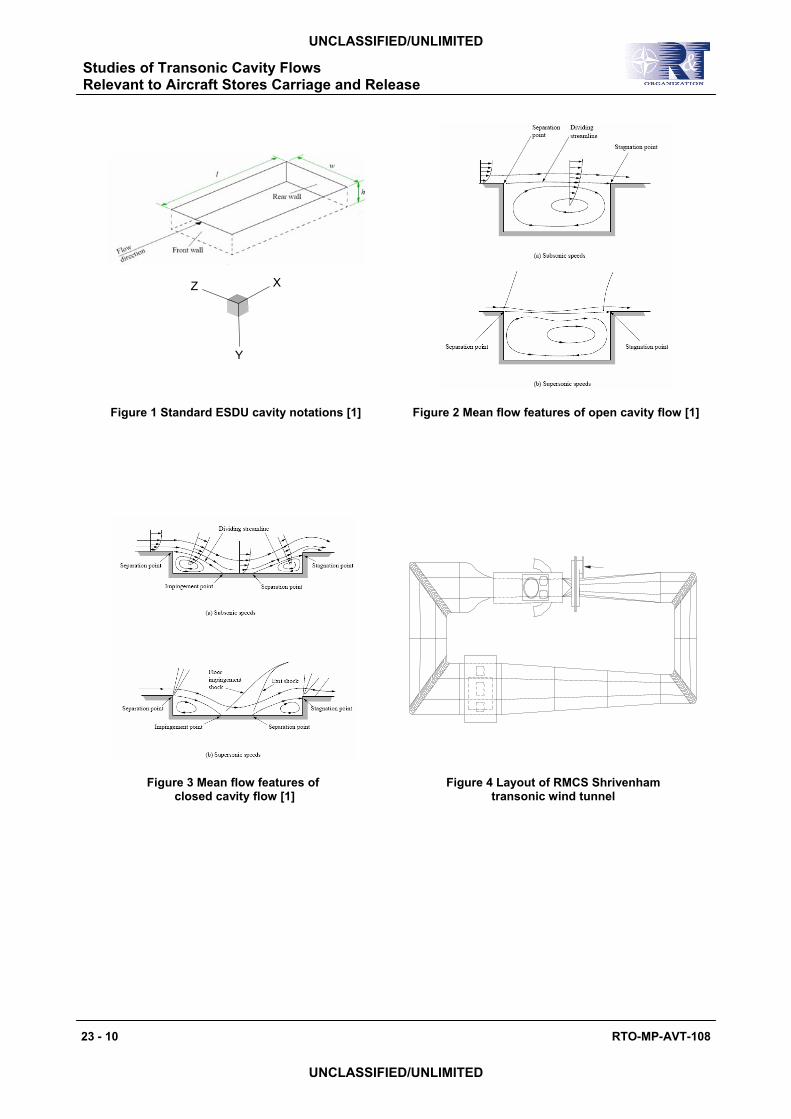
A custom-built seeding system injected water particles of 5-10µm diameter into the contraction section to seed the flow (Figure 5a). The seeder supplied a rake of three splash-plate atomiser nozzles with water pressurised to 2000psi.

2.2 PIV System The PIV system consisted of a Dantec FlowMap 500 hardware box, a Kodak ES1.0 megapixel CCD camera and a New Wave Gemini Nd:YAG double pulsed laser. The Kodak ES1.0 camera frame rate and laser repetition rate allowed data to be recorded at up to 15Hz. The light sheet was projected into the cavity through the glass floor and was oriented along the cavity centreline. The seeded light sheet was


RTO-MP-AVT-108 23 - 3



viewed via a surface coated mirror angled at 45° to the cavity right side wall which provided a field of view normal to the light sheet. The exact details if the set up can be seen in Figure 5b. PIV data processing was initially undertaken using TSI’s Insight software, which uses the Hart algorithm [11]. The data were also processed using an in-house code based on the correlation algorithm proposed by Meinhart et al [12]. The in-house code produces time-averaged flow fields only, but has the advantage of averaging the correlation peaks in each interrogation region instead of averaging the resulting vectors. This different approach to time averaging the data results in a higher signal to noise ratio from data where seeding levels are low. However, the resolution of this technique is reduced compared with the Hart algorithm which, given a suitable image with high seeding levels, can extract multiple vectors from each interrogation region. Table 1 lists the details of the processing variables for the different cavity geometries tested.

Cavity Geometry l/h=5 l/h=14

TSI Primary Correlation Window Size (pixels) 32x32 16x16

TSI Secondary Correlation Window Size (pixels) 16x16 8x8

TSI Maximum Search Length (pixels) 8 8

TSI Vectors per Image 9600 3904

In-house Primary Correlation Window Size

(pixels) 32x32 16x16

In-house window overlap (pixels) 24 4

In-house Maximum Search Length (pixels) 8 4

In-house Vectors per Image 1464 450

Table 1 PIV Processing Details

3.0 NUMERICAL MODELLING

Computational modelling was performed using the commercially-available CFD code Fluent. Computational grids of the cavity geometries were constructed using the grid-generation package GAMBIT. The domains for the cavities were sized at 500mm long to correspond to the size of the test rig flat plate and 230mm high to correspond to the TWT test section width.

The predictions were made using the segregated implicit solver with the realizable k-ε turbulence model. This particular turbulence model was chosen as it has been previously used in a number of studies involving flows with high shear and regions of recirculation and has been shown to be more effective for flows with regions of flow impingement and recirculation than the standard k-ε model [13]. The segregated implicit solver was chosen over the coupled implicit solver as it is less memory intensive and hence solutions can be attained more quickly. The segregated solver also offers better convergence performance than the coupled solver for the cases considered. The CFD predictions were computed on Linux workstations and with the available resources a single time step was computed in approximately 20-25 seconds.


23 - 4 RTO-MP-AVT-108



4.0 RESULTS

4.1 PIV Data The PIV system acquires a maximum of 70 image pairs per tunnel run at 15Hz sampling rate which is equivalent to the maximum laser refresh rate. These datasets were processed into instantaneous vector maps and then into mean vector maps using the TSI code and directly into mean vector maps using the in-house code. The flow data were compared with the time-averaged URANS CFD predictions. Given a sample size of N = 70 and the random nature of the PIV sample, statistically the results will have a 12% uncertainty in the mean vector values as the component of uncertainty falls as 1/√N [14]. In order to reduce the uncertainty in the measurements, the image pairs from a number of tunnel runs were added together to generate the time-averaged vector maps from a much larger number of samples. Based on a sample size of N=700 image pairs, the uncertainty in the measurement has been reduced from 12% to 3.7%.

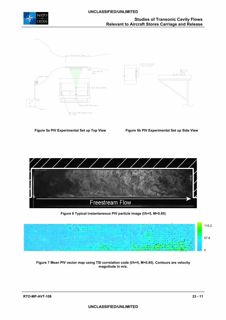
A typical instantaneous image for the plane of symmetry of the l/h=5 cavity can be seen in Figure 6. Note the low seeding density near the upstream wall which is attributed to a region of ‘dead’ flow into which seeding cannot be effectively carried. All PIV and CFD flow fields are oriented as per this particle image.

4.1.1 Open Cavity (l/h=5)

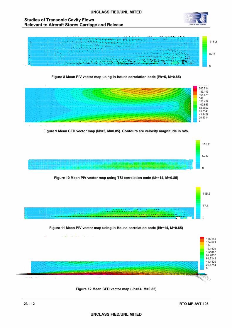
As previously stated, time-averaged flow fields were extracted from the PIV data using the commercial TSI correlation code and an in-house correlation code. The resultant vector maps for the commercial and in-house codes can be seen in Figures 7 and 8 respectively. The number of vectors in the figures has been reduced by 50% to increase the clarity of the flow structures. In both cases the structure of the flow field closely matches the expected large single recirculation region which is characteristic of the mean flow field in an open cavity. The low concentration of seeding in the upstream region of the cavity affects the quality of data extracted by the TSI code but has a lesser effect on the data processed with the in-house code due to the nature of the algorithm. The position of the centre of recirculation within the cavity is extracted at slightly different locations. The TSI code shows the centre of recirculation to be positioned at x/l=0.4 whilst the in-house code shows the centre to be positioned x/l=0.5. The shear layer which bridges the cavity is visibly deflected into the cavity near the downstream wall and as a result the flow in this region is faster than elsewhere in the cavity.

4.1.2 Closed Cavity (l/h=14)

The time-averaged flow fields extracted from the l/h=14 PIV data can be seen in Figures 10 and 11 for the TSI and in-house codes respectively. Examination of the flow field structure for the two data sets shows that the flow exhibits good similarity to the expected mean flow field described in the literature. The flow enters the cavity and traps a region of expanded flow in the upstream half of the cavity before flowing along the cavity floor between x/l=0.5-0.7 and then turning out of the cavity near the downstream end and trapping a small region of compressed flow.

4.2 Time-averaged CFD Data The time-averaged CFD flow fields are constructed from 20000 time steps of 5µs to give 0.1 seconds of flow time for both the l/h=5 and l/h=14 cases.

4.2.1 Open Cavity (l/h=5)

The time-averaged flow field for the l/h=5 case can be seen in Figure 9. The flow field displays a large single recirculation region within the cavity which is expected from the literature and is consistent with the PIV flow fields. However, the CFD flow field has a region of flow on the floor near the downstream wall


RTO-MP-AVT-108 23 - 5



in which the flow velocity is much greater than that extracted from the PIV data. This increased flow velocity is due to the addition of mass to the cavity at the downstream wall when the shear layer dips below the level of the trailing edge. The flow in the first 15% of the cavity length is very low speed compared to elsewhere in the cavity. This is consistent with the PIV data showing that the recirculation does not fill the entire cavity. Literature suggests that the flow in this region contains a contra-rotating vortex although this is not confirmed or otherwise by the PIV and CFD data.

4.2.2 Closed Cavity (l/h=14) The time-averaged flow field for the l/h=14 cavity can be seen in Figure 12. The flow structure is consistent with that expected from the literature. A region of flow is present on the cavity floor from 10-60% of the cavity length which is of increased velocity compared with the surrounding flow. This is not present in the PIV data; however, this may be due to the high spatial gradient in this region adversely affecting the data extracted from the PIV images.

5.0 DISCUSSION In order to quantitatively compare the PIV and CFD data from the three flow fields, profiles of the streamwise and vertical velocity components were extracted along the cavity at y/d=0.25 (75% of cavity height from floor), y/d=0.5 (50% of cavity height from floor) and y/d=0.75 (25% of cavity height from floor).

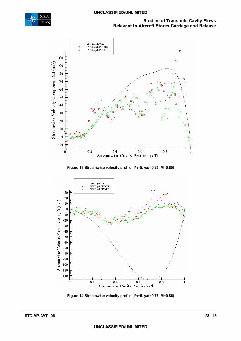
5.1 l/h=5 Cavity Figures 13 and 14 show the u velocity component from the cavity at y/d=0.25 and y/d=0.75 respectively. At y/d=0.25 the peak velocity extracted by the TSI code closely matches the CFD predicted velocity in terms of both value and position. The in-house code shows peak values of approximately 60ms-1 which is 7% of freestream values (≈20ms=1) less than the TSI and CFD values. It can be seen from the three vector fields that the CFD predicts the recirculation centre at x/l=0.7 whilst the two PIV codes show the centre of recirculation to be located between x/l=0.4-0.5.

The CFD predicts peak velocities up to -125m-1 in u at y/d=0.75. The region of increased flow velocity on the floor near the downstream wall in the CFD prediction is not mirrored in the PIV data which suggests that the large increase In flow velocity as the flow travels down the downstream wall and the large decrease in flow velocity as the flow travels upstream along the cavity floor cannot be extracted from the PIV data. Keane and Adrian [15] recommend that a seeding particle should travel no further than 25-30% of the interrogation window size between laser pulses in order to extract high quality data. However, in flows with a high degree of shear and swirl, large velocity gradients may exist which apply large accelerations on the seeding particles. This means that in the high shear regions, the particles may travel further than the recommended 25-30% between frames which prevents them being correlated together as the algorithm will only search to a maximum length of 25% of the interrogation region size. A balance must be met between the maximum expected velocity and the selected laser pulse separation in order to ensure that particle displacement between frames is within the optimum 25-30% of region size over the majority of the cavity. This may mean however, that some flow features are incorrectly extracted; this seems to be the case in the region along the cavity floor.

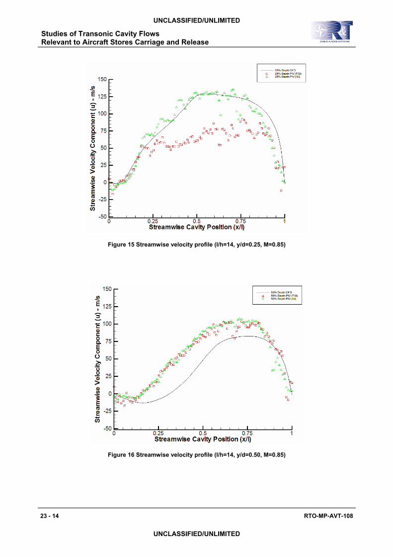
5.2 l/h=14 Cavity Figures 15 and 16 show the u velocity component profiles at y/d=0.25 and y/d=0.5. The streamwise velocity profiles extracted from the three datasets all show close agreement in terms of the trends described by the data. At y/d=0.25, the CFD and the PIV data processed with the in-house code show excellent agreement in trend and velocity values whilst the TSI processed data follows the trend but the velocity values are up to 24% of freestream values (≈70ms-1) lower than the CFD and in-house PIV values.


23 - 6 RTO-MP-AVT-108



At y/d=0.5, the PIV data and the CFD data follow similar trends however, the CFD peak velocities are approximately 10% of freestream values lower (≈25-30ms-1) than the values extracted from the PIV data.

5.3 General Comparison of the flow structures and velocity trends for the two different cavity geometries shows that whilst the PIV technique is capable of extracting the mean flow structure accurately, the velocities which can be extracted are affected by the limitations of the processing code in terms of maximum particle displacement and high levels of swirl and shear.

Improvements to the PIV data can be made using the current two processing codes by dividing the flow field into a number of regions based upon the expected flow velocities. These regions can then be processed with different maximum displacement criteria to try and extract the actual flow field more effectively. This technique may help to improve the flow velocity values within the cavity, however, complex flow structures may still remain difficult to extract successfully. A correlation code is available which deforms the interrogation window in the second frame of an image pair in order to try and follow strong spatial gradients within the flow.

PIV measurements in high-speed flows with high frequency phenomena such as open cavity flows, which lead to rapid changes in speed and direction, may suffer from delay in the response of the seeding to these changes. This can cause measured peak velocities to be artificially reduced. Dring [16] provides a method to estimate the error in velocity caused by the seeding lag for either a step deceleration or an exponential acceleration. For example, with seeding particles between 5-10µm in diameter, a particle density of 1000kgm-3 and an exponential acceleration from 20-150ms-1 in 20mm (which is representative of the flow velocity increase near the downstream wall of the open cavity), the particle Stokes number will vary from 0.009 to 0.036 which corresponds to a predicted error of 6 to 10%.

The acquisition of PIV data from cavity flows at transonic speeds has proved to be most challenging in terms of both rig design and data acquisition. The RMCS TWT layout is such that major alterations to improve optical access are not possible. Any improvement in access for lasers had to be achieved through the design of the cavity rig.

Access for light sheet and imaging optics in the RMCS TWT is highly restricted due to the size of the tunnel test section. Hence PIV rig design is limited to attaching a fully or partially clear cavity to the outside of the tunnel wall as in the current design (Fig 5). The highly unsteady nature of the flow within the open cavity has proved to be difficult to capture with the image acquisition refresh rates available. The current capture rate of the CCD camera and Nd:YAG laser used for image acquisition is limited to 15Hz and as such is too low to fully resolve the flow structures associated with dominant frequencies of oscillation. Estimates from the modified Rossiter equation [17] place the frequencies of the first three modes of oscillation for the open cavity case at 460Hz, 1125Hz and 1795Hz. A time-resolved or cinematic PIV system with laser and camera repetition rates in the order of 2kHz would be required to properly resolve the first two frequencies of oscillation expected within the cavity.

5.4 Comparisons with previous work Previous published studies relating to non-intrusive measurements of cavity flows are limited to work conducted by Esteve et al [18] and Unalmis et al [19]. In the first case, the PIV studies were conducted at low subsonic flow speeds and in the second case the measurements were restricted to flow visualisation using planar laser scattering (PLS). As such no direct comparisons can be made between previous work and the results presented here; it is believed no equivalent PIV studies for closed and transitional cavities at transonic speeds have been published in the open literature to date.


RTO-MP-AVT-108 23 - 7



A considerable number of computational studies have been dedicated to modelling the flow over cavities at transonic speeds. A survey conducted by Grace [20] into computational techniques for cavity flow noise prediction covered many of the main studies to date. A more recent study of note includes predictions for an l/h=5 cavity for the same flow conditions as the current test conducted by Lawrie et al [21] using the SST k-ω turbulence model. The results from this study have been used as a basis for the development of the solutions contained within the current cavity flow study.

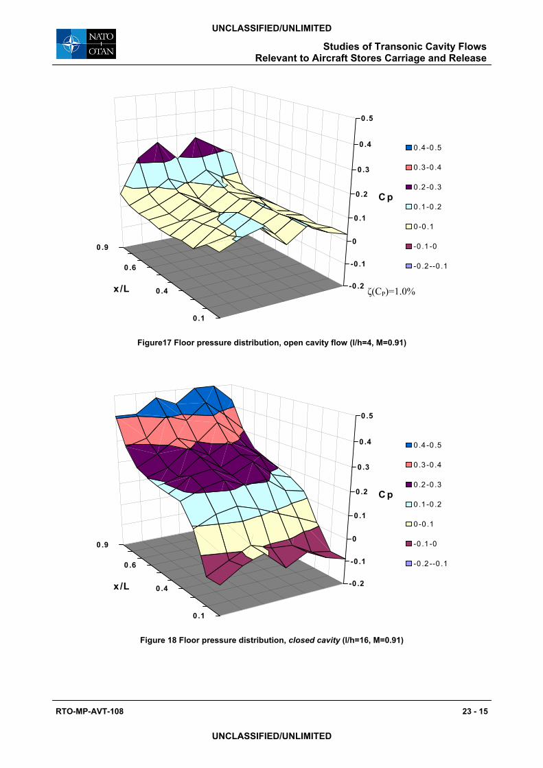
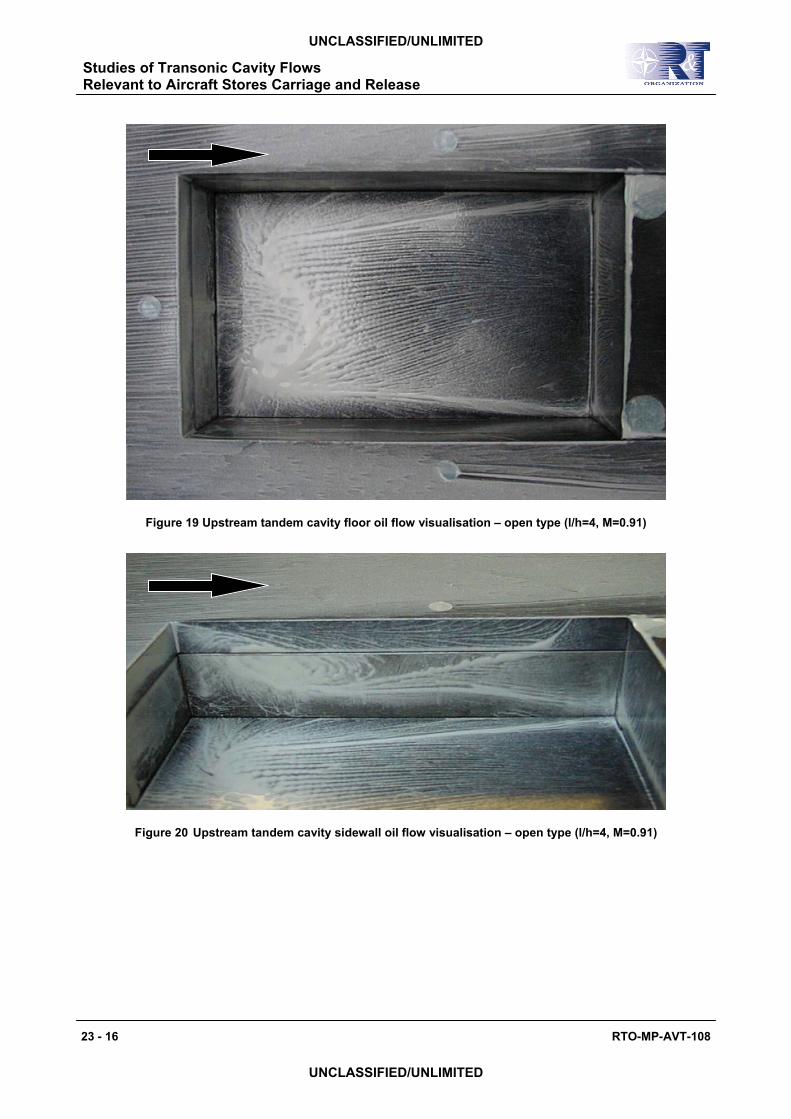
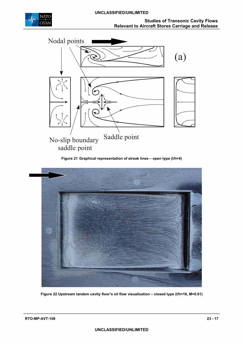
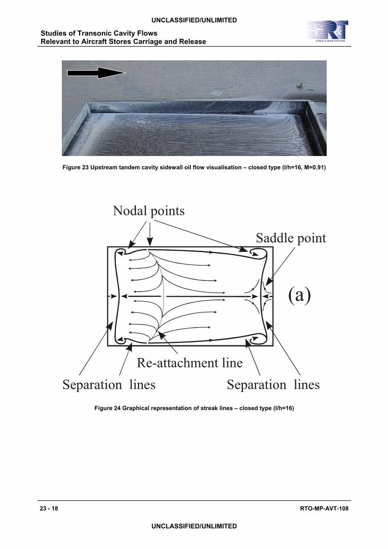
5.5 Three-dimensional and unsteady features The present PIV results have been confined to the plane of symmetry of a three-dimensional cavity and compared with 2-D CFD simulations. As identified above, there are some discrepancies due to the 3-D nature of the experimental flow. We have also explored this three-dimensionality in more detail using surface pressure measurements, oil flow visualisation and fully 3-D CFD simulations. This experimental work was carried out at a freestream Mach number of 0.91 as part of a study of tandem cavities [22]. Pressure distributions are shown in Figures 17 & 18 for open and closed cases respectively. Figures 19, 20, 22 & 23 show surface oil flow visualisation for these cases. These surface flows are interpreted in Figures 21 & 24. It is clear that the l/h=4 case is highly three-dimensional, whereas at l/h=16 much of the cavity experiences a fairly uniform, quasi-2-D flow, with three-dimensionality largely limited to the sidewall regions.

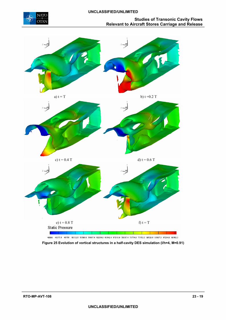
The three-dimensionality of the open cavity flows are further emphasised by the CFD results of Figure 25. This figure was produced using Detached Eddy Simulation and shows a sequence of frames representing the evolution of a vorticity isosurface (ξ=22000rad/s) in a half width of the cavity, for different instants along one oscillation period (T). The colouring of the surfaces corresponds to the static pressure values at the surface of the isocontour. As well as revealing spanwise variations in the flow these plots also highlight the unsteady nature of open cavity flows. Figure 25b represents the cavity after the impingement of a shear layer vortex and shows the formation of a pressure wave, identified by the red colour zone in the isosurface. It is possible to observe the pressure wave travelling upstream along the cavity. This is then responsible for the upward deflection of the shear layer (Figure 25e). This theory is supported by Heller and Bliss [23] – the idea of a pressure driven oscillation mechanism. It is also possible to observe vorticity lumps being shed by the shear layer and travelling downstream along the cavity centreline, these vorticity lumps correspond to vortices that travel downstream alternately with tubular vortical structures formed in the beginning of the lateral edge of the cavity. These grow while travelling downstream along this edge, providing a 2-1-2 superficial mode of oscillation to the shear layer. These tubular vortical structures are triggered by a low-to-high pressure field; this induces a rotation in the flow plane along the lateral edge of the cavity. This occurs just after the upstream edge, when the shear layer is deflected to the interior of the cavity.

6.0 CONCLUSIONS

For the first time, time-averaged PIV and CFD results have been presented for open and closed cavity flows at transonic speeds. The comparison of time-averaged PIV data with URANS CFD predictions has proved the ability of PIV to be used as a tool for the analysis of the complex flow structures associated with cavity flows at transonic speeds. Whilst flow structures can be extracted using PIV, traditional correlation codes in which the interrogation window shape is fixed cannot extract data from regions containing high spatial gradients. This is most apparent in the l/h=5 cavity where the high speed flow region on the floor, which is predicted by the CFD, is not extracted from the PIV images. This limitation of the two codes used for this study can be overcome with the use of a new development in correlation codes whereby the interrogation region is deformed in order to more effectively track large particle displacements due to spatial gradients [24].


23 - 8 RTO-MP-AVT-108



More detailed work is required to improve these results. The current study has shown that PIV can be used as a means for detailed analysis of cavity flows providing due attention is paid to optical access and seeding quality. Based on the PIV data processed for the current study, it is clear that whilst the results from time-averaged flow fields produce vector maps with flow structures similar to those defined in the cavity flow literature, the instantaneous vector maps are captured at too low a frame rate to be able to extract frequency information from the cavity. This can only be properly addressed by either ‘phase-locking’ the PIV acquisition to each of the oscillation frequencies or using a high speed PIV system with a minimum of 2-3kHz capture rate to acquire time resolved flow data. Whilst ‘phase-locked’ acquisition can successfully extract flow data for a single frequency phenomenon, flows in which multiple frequencies of oscillation exist cannot be fully analysed. This suggests that future studies of ‘open’ cavity flows should be undertaken with high-speed PIV systems which can extract full time-wise behaviour from flows with multiple frequencies of oscillations.

ACKNOWLEDGEMENTS

The authors would like to thank the EPSRC and MBDA UK Ltd for their support of some of this work under the CASE award scheme. We would also like to thank Dr John Coath, Mr Roy Walker and Dr Mark Finnis of the department of Aerospace, Power and Sensors and the workshops of the Engineering Systems Department at Shrivenham for their assistance with various aspects of this work.

REFERENCES

[1] ESDU, (2002), "Drag of a rectangular planform cavity in a flat plate with a turbulent boundary layer for Mach numbers up to 3. Part II : Open and transitional flows", ESDU 00007,

[2] Charwat, A. F., Roos, J. N., Dewey, F. C., Jr., and Hitz, J.A (1961): J. Aerosp. Sci., vol. 28,no.6, June, pp. 457—470.

[3] Stallings, R.J., et al., (1995) “Measurements of Store Forces and Moments and Cavity Pressures for a Generic Store in and Near a Box Cavity at Subsonic and Transonic Speeds” NASA TM-4611. NASA.

[4] Taborda, N.M., D. Bray, and K. Knowles, (2001) "Passive Control of Cavity Resonances in Tandem Configurations", 31st AIAA Fluid Dynamics Conference, Anaheim, CA, 11-14 June 2001. Paper no. AIAA 2001-2770.

[5] Taborda, N., D. Bray, and K. Knowles, (2001) “Visualisation of Three-dimensional Cavity Flows”, in 5th World Conference on Experimental Heat Transfer, Fluid Mechanics and Thermodynamics. Thessaloniki, Greece.

[6] Garg, S. and L.N. Cattafesta III, (2001) “Quantitative Schlieren Measurements of Coherent Structures in a Cavity Shear Layer”, Experiments in Fluids, (30): p. 123-134.

[7] Sinha, N., et al. (1998) “A Perspective on the Simulation of Cavity Aeroacoustics”, in 36th Aerospace Sciences Meeting and Exhibit. Reno, NV.

[8] Zhang, J., et al. (2001) “Experimental and Computational Investigation of Supersonic Cavity Flows”, in 10th AIAA/NAL-NASDA-ISAS International Space Planes and Hypersonic Systems and Technologies Conference. Tokyo.

[9] Adrian, R.J., (1991) “Particle Imaging Techniques for Experimental Fluid Mechanics”, Annual Review of Fluid Mechanics, (23): p. 261-304.


RTO-MP-AVT-108 23 - 9



[10] Lawson N.J., Page G., Halliwell N.A., Coupland J.M. (1999) "Application of Particle Image Velocity to a Small Scale de Laval Nozzle", AIAA Journal 37(7), p798-804.

[11] Hart, D., (2000), "PIV error correction." Experiments in fluids, 29, 13-22

[12] Meinhart, C., Wereley, S., and Santiago, J., (2000), "A PIV Algorithm for Estimating Time-Averaged Velocity Fields." Journal of Fluids Engineering (122), 285-289.

[13] Prepared by WS Atkins Consultants and Members of the NSC (2002), "Best Practice Guidelines for Marine Applications of Computational Fluid Dynamics" http://pronet.wsatkins.co.uk/marnet/guidelines/guide.html/

[14] Coleman, H., and Steele, W., (1999), Experimentation and uncertainty analysis for engineers, John Wiley and Sons, Inc., New York.

[15] Keane, R., and Adrian, R., (1990), "Optimization of Particle Image Velocimeters. Part I: Double Pulsed Systems." Measurement Science and Technology, 1, 1202-1215.

[16] Dring, R., (1982), "Sizing criteria for laser anemometry particles." Journal of Fluids Engineering, 104, 15-17.

[17] Rossiter, J. E., (1964), "Wind tunnel experiments on the flow over rectangular cavities at subsonic and transonic speeds." Royal Aircraft Establishment.

[18] Esteve, M. J., Reulet, P., and Millan, P., (2000), "Flow field characterisation within a rectangular cavity", 10th International Symposium on the Applications of Laser Technology to Fluid Mechanics, Lisbon, Portugal.

[19] Unalmis, O. H., Clemens, N. T., and Dolling, D. S., (1999), "Planar Laser Imaging of a Supersonic Side Facing Cavity", 37th AIAA Aerospace Sciences Meeting and Exhibit, Reno NV, January 11-14 1999.

[20] Grace, S., (2001), "An Overview of Computational Aeroacoustic Techniques Applied to Cavity Noise Prediction", 39th AIAA Aerospace Sciences Meeting and Exhibit, Reno, NV.

[21] Lawrie, D., Nayyar, P., Badcock, K., Barakos, G., and Richards, B., (2003), "CFD Study of Cavity Flows", CEAS Aerospace Aerodynamics Research Conference, London, UK, 10-12 June 2003.

[22] Taborda, N.M.L. (2003) “Rectangular Tandem Cavities at Transonic Speeds”, PhD Thesis, Cranfield University, College of Defence Technology, Shrivenham.

[23] Heller, H. H. and D. B. Bliss (1975). The Physical Mechanism of Flow Induced Pressure Fluctuations in Cavities and Concepts for Suppression. A/M 2nd Aeroacoustics Conference, AIAA.

[24] Scarano, F., (2002), "Iterative Deformation Methods in PIV." Measurement Science and Technology, 13, R1-R19.

http://pronet.wsatkins.co.uk/marnet/guidelines/guide.html/


23 - 10 RTO-MP-AVT-108



X

Y

Z

Figure 1 Standard ESDU cavity notations [1]

Figure 2 Mean flow features of open cavity flow [1]

Figure 3 Mean flow features of closed cavity flow [1]

Figure 4 Layout of RMCS Shrivenham transonic wind tunnel


RTO-MP-AVT-108 23 - 11



Figure 5a PIV Experimental Set up Top View

Figure 5b PIV Experimental Set up Side View

Figure 6 Typical instantaneous PIV particle image (l/h=5, M=0.85)

115.2

57.6

0

Figure 7 Mean PIV vector map using TSI correlation code (l/h=5, M=0.85). Contours are velocity magnitude in m/s.


23 - 12 RTO-MP-AVT-108



115.2

57.6

0

Figure 8 Mean PIV vector map using In-house correlation code (l/h=5, M=0.85)

226.286205.714185.143164.571144123.429102.85782.285761.714341.142920.57140

Figure 9 Mean CFD vector map (l/h=5, M=0.85). Contours are velocity magnitude in m/s.

115.2

57.6

0

Figure 10 Mean PIV vector map using TSI correlation code (l/h=14, M=0.85)

115.2

57.6

0

Figure 11 Mean PIV vector map using In-House correlation code (l/h=14, M=0.85)

185.143164.571144123.429102.85782.285761.714341.142920.57140

Figure 12 Mean CFD vector map (l/h=14, M=0.85)


RTO-MP-AVT-108 23 - 13



Figure 13 Streamwise velocity profile (l/h=5, y/d=0.25, M=0.85)



23 - 14 RTO-MP-AVT-108






RTO-MP-AVT-108 23 - 15



0.1

0 .4

0 .6

0 .9

-0 .2

-0 .1

0

0 .1

0.2

0.3

0 .4

0 .5

C p

x/L

0 .4 -0 .5

0 .3 -0 .4

0 .2 -0 .3

0 .1 -0 .2

0-0 .1

-0 .1 -0

-0 .2 --0 .1

Figure17 Floor pressure distribution, open cavity flow (l/h=4, M=0.91)

0 .1

0 .4

0 .6

0 .9

-0 .2

-0 .1

0

0 .1

0.2

0.3

0 .4

0 .5

C p

x/L

0 .4 -0 .5

0 .3 -0 .4

0 .2 -0 .3

0 .1 -0 .2

0-0 .1

-0 .1 -0

-0 .2 --0 .1

Figure 18 Floor pressure distribution, closed cavity (l/h=16, M=0.91)

ζ(CP)=1.0%


23 - 16 RTO-MP-AVT-108



Figure 19 Upstream tandem cavity floor oil flow visualisation – open type (l/h=4, M=0.91)

Figure 20 Upstream tandem cavity sidewall oil flow visualisation – open type (l/h=4, M=0.91)


RTO-MP-AVT-108 23 - 17



Nodal points

No-slip boundary saddle point

Saddle point

(a)

Figure 21 Graphical representation of streak lines – open type (l/h=4)

Figure 22 Upstream tandem cavity floor’s oil flow visualisation – closed type (l/h=16, M=0.91)


23 - 18 RTO-MP-AVT-108



Figure 23 Upstream tandem cavity sidewall oil flow visualisation – closed type (l/h=16, M=0.91)

Nodal points

Saddle point

Re-attachment lineSeparation lines Separation lines

(a)

Figure 24 Graphical representation of streak lines – closed type (l/h=16)


RTO-MP-AVT-108 23 - 19



a) t = T b) t =0.2 T

c) t = 0.4 T d) t = 0.6 T

e) t = 0.8 T f) t = T

Figure 25 Evolution of vortical structures in a half-cavity DES simulation (l/h=4, M=0.91)


23 - 20 RTO-MP-AVT-108



DISCUSSION EDITING

Paper No. 23: Studies of Transonic Cavity Flows Relevant to Aircraft Stores Carriage and Release

Authors: K. Knowles, N .J. Lawson, D. Bray, S.A. Ritchie and P. Geraldes

Speaker: Kevin Knowles

Discussor: Kit Eaton

Question: You described problems with seeding. The cavity flow and how you had built a seeding device for injecting water. What velocity/mass flows did this use relative to those that have ????shown to modify the cavity flow.

Speaker’s Reply: The seeder has an outlet of about 200 m/s; this jet then strikes an impact plate to produce a cloud of micron-size droplets. This cloud is then carried along by the wind tunnel flow. This design of seeder could not be easily integrated with our small, transparent cavity without affecting the flow. We have preferred to introduce alternative PIV signal processing techniques to address regions of low signal-to-noise.

Discussor: Fred Mendonca

Question: Simulations done in 3D but assuming symmetry constrain a symmetrical flow about this plane.

Our own 3D simulations suggest a snaking flow which is non-symmetrical.

Was the asymmetry obscured in the measurements?

Speaker’s Reply: We have not yet seen this but will examine or data to see if there si any evidence for this phenomenon.

Documents

Studies of Transonic Cavity Flows - NATO Meeting Proceedings/RTO... · Cranfield University, RMCS Shrivenham ... School of Engineering, Cranfield University, Cranfield, ... Studies