Embed Size (px)
Citation preview
Studies into tau reconstruction, missing transverse energy
and photon induced processes with the ATLAS detector at
the LHC
Dissertation
zur
Erlangung des Doktorgrades (Dr. rer. nat.)
der
Mathematisch-Naturwissenschaftlichen Fakultat
der
Rheinischen Friedrich-Wilhelms-Universitat Bonn
vorgelegt von
Robindra P. Prabhu
aus
Oslo, Norwegen
Bonn 2010


Angefertigt mit Genehmigung der Mathematisch-Naturwissenschaftlichen Fakultat der
Rheinisch Friedrich-Wilhelms-Universitat Bonn
1. Gutachter: Prof. Dr. Klaus K. Desch
2. Gutachter: Prof. Dr. Jochen Dingfelder
Tag der Promotion: 27. Oktober 2010
Erscheinungsjahr: 2011


Abstract
The ATLAS experiment is currently recording data from proton-proton collisions de-
livered by CERN’s Large Hadron Collider. As more data is amassed, studies of both
Standard Model processes and searches for new physics beyond will intensify. This
dissertation presents a three-part study providing new methods to help facilitate these
efforts.
The first part presents a novel τ -reconstruction algorithm for ATLAS inspired by the
ideas of particle flow calorimetry. The algorithm is distinguished from traditional τ -
reconstruction approaches in ATLAS, insofar that it seeks to recognize decay topologies
consistent with a (hadronically) decaying τ -lepton using resolved energy flow objects
in the calorimeters. This procedure allows for an early classification of τ -candidates
according to their decay mode and the use of decay mode specific discrimination against
fakes. A detailed discussion of the algorithm is provided along with early performance
results derived from simulated data.
The second part presents a Monte Carlo simulation tool which by way of a pseudorapidity-
dependent parametrization of the jet energy resolution, provides a probabilistic estimate
for the magnitude of instrumental contributions to missing transverse energy arising
from jet fluctuations. The principles of the method are outlined and it is shown how the
method can be used to populate tails of simulated missing transverse energy distributions
suffering from low statistics.
The third part explores the prospect of detecting photon-induced leptonic final states in
early data. Such processes are distinguished from the more copious hadronic interactions
at the LHC by cleaner final states void of hadronic debris, however the soft character of
the final state leptons poses challenges to both trigger and offline selections. New trigger
items enabling the online selection of such final states are presented, along with a study
into the feasibility of detecting the two-photon exchange process pp(γγ → ττ)p∗p∗ with
early data.
iii

Acknowledgements
Over the last few years, I have had the great fortune to interact with a number of
remarkable people without whose guidance, insight, perspectives and sharing of ideas
this work would likely never have seen the light of day.
I warmly thank Prof. Dr. Klaus Desch for ”taking me under his wings”, for the op-
portunity to work on a range of different topics and for providing me with the space to
develop and mature and bring the ideas presented herein to fruition. His encouragement,
patience and support has been greatly appreciated.
I am equally grateful to Peter Wienemann, for the countless discussions we have had
on physics and equally often on topics far beyond. His impressive insight and clarity
of thought has been an invaluable resource to me throughout and a constant source of
wonder and amazement.
I must also thank Sebastian Fleischmann and Mark Hodgkinson for the fruitful collabo-
ration on the development of PanTau. Their ideas and contributions were instrumental
to parts of the work presented in Chapter 2 and I am thankful for all that they have
taught me along the way.
I am grateful for the encouragement, constructive critizisms and many helpful comments
provided by both Wolfgang Mader and Yann Coadou in their capacity as conveners for
the ATLAS Tau Working Group during my stay at CERN. Frank Paige, Shoji Asai
and Dan Tovey also deserve mention for their friendly and helpful input to the studies
presented in Chapter 3.
I am hugely indebted to Andrew Hamilton for enthusiastically sharing his expertise on
two-photon physics at hadron colliders and to Andrew Pilkington, Olya Igonkina, Anna
Sfyrla and Stefania Xella for all their help and assistance with the ATLAS trigger. A
big word of thanks also to Christian Limbach for enthusiastically carrying the torch
onwards.
I would go amiss if I failed to acknowledge the efforts of all the people who have pro-
vided invaluable technical support during the course of this work: Michael Heldmann
and Michael Duhrssen for introducing me to the ATLAS software and for patiently an-
swering all my tedious questions during my early months in Freiburg. The ”Bonner”
administrators have always been equally friendly, accommodating and quick to answer
queries. Last but not least, I am indebted to Wolfgang Ehrenfeld and the NAF support
team for accommodating all my computing needs over the last few years.
I wish to thank all members of the HEP groups in Freiburg and Bonn for the good
company and friendly atmosphere, especially all the people with whom I have at one
point or another shared an office. The ”Kochgruppe” at CERN should not be forgotten,
thank you all for making my stay at CERN all the more enjoyable. I am indebted to Peter
Wienemann and Carolin Zendler for lending their keen eyes to the proof-reading of this
manuscript and for the many helpful comments they both provided. Frau Furstenberg
iv

and Frau Streich also both deserve a special mention for the countless occasions on which
they have extended a helpful hand.
Warm and heartfelt thanks to Carolin, Duc, Giacinto, Gisela, Henrik, Michael, Natalia,
Olav and Zong for all the good times we have shared and for making the past few years
all the more enjoyable and worthwhile.
Finally, I wish to thank my dearest parents for their unwavering support and encour-
agement through thick and thin.

To my parents.
vi

Contents
Abstract iii
Acknowledgements iv
Symbols and abbreviations xi
1 Introduction 1
1.1 Preface . . . . . . . . . . . . . . . . . . . . . . . . . . . . . . . . . . . . . 1
1.2 The Large Hadron Collider and its experimental environment . . . . . . . 4
1.2.1 The LHC machine . . . . . . . . . . . . . . . . . . . . . . . . . . . 5
1.2.2 Early data prospects . . . . . . . . . . . . . . . . . . . . . . . . . . 8
1.3 The phenomenology of proton-proton collisions . . . . . . . . . . . . . . . 9
1.3.1 Anatomy of hadronic interactions at the LHC . . . . . . . . . . . . 10
1.3.2 The hard interaction . . . . . . . . . . . . . . . . . . . . . . . . . . 12
1.3.3 From hard scattering to experimental observables . . . . . . . . . . 14
1.3.3.1 Parton showers . . . . . . . . . . . . . . . . . . . . . . . . 14
1.3.3.2 Hadronization . . . . . . . . . . . . . . . . . . . . . . . . 15
1.3.4 Photon interactions in proton-proton collisions . . . . . . . . . . . 17
1.3.4.1 Theoretical description of photon interactions at hadroncolliders . . . . . . . . . . . . . . . . . . . . . . . . . . . . 18
1.3.5 The underlying event . . . . . . . . . . . . . . . . . . . . . . . . . 20
1.3.6 Pile-up and Minimum Bias . . . . . . . . . . . . . . . . . . . . . . 22
1.4 The ATLAS experiment . . . . . . . . . . . . . . . . . . . . . . . . . . . . 24
1.4.1 The central detector systems . . . . . . . . . . . . . . . . . . . . . 25
1.4.1.1 The innermost tracking detectors . . . . . . . . . . . . . 26
1.4.1.2 The calorimetry . . . . . . . . . . . . . . . . . . . . . . . 29
1.4.1.3 The Muon Spectrometer . . . . . . . . . . . . . . . . . . 33
1.4.2 The forward detector systems . . . . . . . . . . . . . . . . . . . . . 35
1.4.2.1 MBTS (z= ±3.6 m, 2.12< |η| < 3.85) . . . . . . . . . . . 35
1.4.2.2 LUCID (z=±17 m, 5.4< |η| <6.1) . . . . . . . . . . . . . 37
1.4.2.3 ZDC (z=±140 m, |η| >8.3) . . . . . . . . . . . . . . . . . 38
1.4.2.4 ALFA (z=±240 m, 10.6< |η| <13.5) . . . . . . . . . . . . 38
1.4.2.5 AFP - ATLAS Forward Proton Project . . . . . . . . . . 38
1.5 Trigger and Data Acquisition . . . . . . . . . . . . . . . . . . . . . . . . . 39
vii

Contents
1.6 A note on Monte Carlo simulations . . . . . . . . . . . . . . . . . . . . . . 41
2 Tau Reconstruction and Identification 43
2.1 Introduction . . . . . . . . . . . . . . . . . . . . . . . . . . . . . . . . . . . 43
2.1.1 The decay phenomenology of the τ -lepton . . . . . . . . . . . . . . 43
2.1.2 The role of tau leptons in the LHC physics programme . . . . . . . 45
2.1.3 Kinematics of tau decays at the LHC and challenges to tau recon-struction . . . . . . . . . . . . . . . . . . . . . . . . . . . . . . . . 48
2.2 Conventional approaches to tau reconstruction and identification in ATLAS 50
2.2.1 Tau energy determination . . . . . . . . . . . . . . . . . . . . . . . 51
2.2.2 Tau identification . . . . . . . . . . . . . . . . . . . . . . . . . . . . 52
2.3 The case for energy flow in ATLAS . . . . . . . . . . . . . . . . . . . . . . 52
2.3.1 Clustering of calorimeter cells in ATLAS . . . . . . . . . . . . . . . 54
2.3.1.1 Principle of topological clustering . . . . . . . . . . . . . 54
2.3.1.2 The application of topological clustering to τ -decays . . . 56
2.3.2 Energy flow in ATLAS . . . . . . . . . . . . . . . . . . . . . . . . . 58
2.3.2.1 Determining expected energy deposits . . . . . . . . . . . 59
2.3.2.2 Subtraction of energy deposits . . . . . . . . . . . . . . . 59
2.3.2.3 Recovering split showers . . . . . . . . . . . . . . . . . . . 62
2.3.2.4 Applications to tau reconstruction . . . . . . . . . . . . . 63
2.4 PanTau - particle flow inspired τ -reconstruction . . . . . . . . . . . . . . . 63
2.4.1 The philosophy of PanTau . . . . . . . . . . . . . . . . . . . . . . . 64
2.4.2 General overview . . . . . . . . . . . . . . . . . . . . . . . . . . . . 65
2.4.3 Seeding . . . . . . . . . . . . . . . . . . . . . . . . . . . . . . . . . 68
2.4.3.1 Seed classification performance . . . . . . . . . . . . . . . 69
2.4.3.2 A note on the choice of jet algorithm . . . . . . . . . . . 71
2.4.4 Discrimination against QCD jets . . . . . . . . . . . . . . . . . . . 72
2.4.4.1 The relative composition of the signal within categories . 72
2.4.4.2 The pT dependence of the classification of fakes . . . . . 73
2.4.4.3 Feature classes and feature definitions . . . . . . . . . . . 74
2.4.5 Prong-dependent feature selection . . . . . . . . . . . . . . . . . . 77
2.4.5.1 Category: 1-prong . . . . . . . . . . . . . . . . . . . . . 78
2.4.5.2 Category: 1-prong+neutral . . . . . . . . . . . . . . . . 78
2.4.5.3 Category: 3-prong . . . . . . . . . . . . . . . . . . . . . 80
2.4.5.4 Category: 3-prong+neutral . . . . . . . . . . . . . . . . 80
2.4.5.5 Category: 2-prong . . . . . . . . . . . . . . . . . . . . . 80
2.4.5.6 Category: 2-prong+neutral . . . . . . . . . . . . . . . . 81
2.4.6 Likelihood discriminants and performance evaluation . . . . . . . . 81
2.4.6.1 Transverse energy resolutions . . . . . . . . . . . . . . . . 88
2.4.6.2 Resolving decay resonances . . . . . . . . . . . . . . . . . 91
2.5 Summary . . . . . . . . . . . . . . . . . . . . . . . . . . . . . . . . . . . . 95
3 A method to improve Monte Carlo statistics of QCD induced instru-mental /ET 107
3.1 Calculating /ET in ATLAS . . . . . . . . . . . . . . . . . . . . . . . . . . . 108
3.2 Fake contributions to /ET . . . . . . . . . . . . . . . . . . . . . . . . . . . 109
3.3 Accounting for QCD induced /EfakeT from jet fluctuations . . . . . . . . . . 110

Contents
3.4 The jet imbalance method . . . . . . . . . . . . . . . . . . . . . . . . . . . 111
3.4.1 Parametrizing the jet energy resolution . . . . . . . . . . . . . . . 113
3.4.2 Expected /ET versus reconstructed /ET . . . . . . . . . . . . . . . . 114
3.5 The method applied as a generator filter . . . . . . . . . . . . . . . . . . . 115
3.5.1 Filter rejection and efficiency . . . . . . . . . . . . . . . . . . . . . 115
3.5.2 Filter performance . . . . . . . . . . . . . . . . . . . . . . . . . . . 119
3.5.3 Event kinematics in filtered events . . . . . . . . . . . . . . . . . . 120
3.6 Summary . . . . . . . . . . . . . . . . . . . . . . . . . . . . . . . . . . . . 121
4 Photon-induced exclusive tau final states in early data 123
4.0.1 Two-photon physics at other collider facilities . . . . . . . . . . . . 124
4.0.2 Early two-photon physics at the LHC . . . . . . . . . . . . . . . . 124
4.1 Monte Carlo simulations and event characteristics . . . . . . . . . . . . . 126
4.1.1 Monte Carlo simulations . . . . . . . . . . . . . . . . . . . . . . . . 126
4.1.2 Expected cross sections . . . . . . . . . . . . . . . . . . . . . . . . 127
4.1.3 Event kinematics . . . . . . . . . . . . . . . . . . . . . . . . . . . . 129
4.2 A note on the experimental challenges and assumptions made . . . . . . . 129
4.2.1 Event reconstruction and background suppression . . . . . . . . . 129
4.2.2 Rapidity gaps and proton dissociation . . . . . . . . . . . . . . . . 129
4.2.3 Event pile-up . . . . . . . . . . . . . . . . . . . . . . . . . . . . . . 131
4.2.4 Proton tagging with forward detectors . . . . . . . . . . . . . . . . 131
4.2.5 Trigger . . . . . . . . . . . . . . . . . . . . . . . . . . . . . . . . . 131
4.3 The online selection of exclusive lepton final states . . . . . . . . . . . . . 132
4.3.1 Prospects with default triggers . . . . . . . . . . . . . . . . . . . . 132
4.3.2 Trigger strategy for exclusive leptonic final states . . . . . . . . . . 134
4.3.2.1 Constructing MBTS veto triggers at L1 . . . . . . . . . . 134
4.3.2.2 Constructing new exclusive trigger chains . . . . . . . . . 137
4.3.2.3 Rate evolution with instantaneous luminosity . . . . . . . 139
4.4 Offline object definitions . . . . . . . . . . . . . . . . . . . . . . . . . . . . 140
4.4.1 Muons . . . . . . . . . . . . . . . . . . . . . . . . . . . . . . . . . . 140
4.4.2 Electrons . . . . . . . . . . . . . . . . . . . . . . . . . . . . . . . . 142
4.4.3 Taus . . . . . . . . . . . . . . . . . . . . . . . . . . . . . . . . . . . 143
4.4.4 Jets . . . . . . . . . . . . . . . . . . . . . . . . . . . . . . . . . . . 147
4.4.5 Overlap removal . . . . . . . . . . . . . . . . . . . . . . . . . . . . 147
4.5 Backgrounds . . . . . . . . . . . . . . . . . . . . . . . . . . . . . . . . . . 148
4.5.1 Non-exclusive . . . . . . . . . . . . . . . . . . . . . . . . . . . . . . 148
4.5.2 Exclusive backgrounds . . . . . . . . . . . . . . . . . . . . . . . . . 149
4.5.3 Other background sources . . . . . . . . . . . . . . . . . . . . . . . 151
4.6 Offline selection of the process γγ → ττ . . . . . . . . . . . . . . . . . . . 151
4.6.1 Online trigger selection . . . . . . . . . . . . . . . . . . . . . . . . 152
4.6.2 Offline preselection . . . . . . . . . . . . . . . . . . . . . . . . . . . 152
4.6.2.1 Multiplicity . . . . . . . . . . . . . . . . . . . . . . . . . . 154
4.6.2.2 Exclusivity A . . . . . . . . . . . . . . . . . . . . . . . . . 155
4.6.3 Offline selectors . . . . . . . . . . . . . . . . . . . . . . . . . . . . . 155
4.6.4 Results . . . . . . . . . . . . . . . . . . . . . . . . . . . . . . . . . 157
4.6.5 A note on systematic uncertainties . . . . . . . . . . . . . . . . . . 161
4.7 Extending the reach with heavy ions . . . . . . . . . . . . . . . . . . . . . 161
Contents
4.8 Summary . . . . . . . . . . . . . . . . . . . . . . . . . . . . . . . . . . . . 162
A The ATLAS coordinate system and associated nomenclature 165
B Monte Carlo Event Samples 167
B.1 Chapter 2: PanTau . . . . . . . . . . . . . . . . . . . . . . . . . . . . . . . 167
B.2 Chapter 3: 〈 /ET 〉 . . . . . . . . . . . . . . . . . . . . . . . . . . . . . . . . 167
B.3 Chapter 4: γγ → ττ . . . . . . . . . . . . . . . . . . . . . . . . . . . . . . 169
B.3.1 Exclusive signal and exclusive backgrounds . . . . . . . . . . . . . 169
B.3.2 Non-exclusive background processes . . . . . . . . . . . . . . . . . 169
C /EfakeT probability distribution function 173
Bibliography 175

Symbols and abbreviations
EFO Energy Flow Object
EFO±q A charged qualified EFO
EFO± A charged EFO (qualified or unqualified)
EFO0EM An electromagnetic neutral EFO
EFO0HAD A hadronic neutral EFO
EFOC An EFO satisfying a criterion C
τvis The visible portion of a τ -lepton decay
τhad A hadronically decaying τ -lepton
τlep A leptonically decaying τ -lepton
τ-induced seed A seed to PanTau originating from a true τ -lepton decay
jet-induced seed A seed to PanTau originating from the hadronisation of quarks and gluons
/ET Reconstructed missing transverse energy
/EfakeT Reconstructed missing transverse energy from instrumental effects
〈 /ET 〉 Total estimated missing transverse energy at the generator level
〈 /EfakeT 〉 Estimated instrumental transverse missing energy at the generator level
xi


Chapter 1
Introduction
1.1 Preface
This document goes into print just as the LHC experiments are presenting some of their
first results from recorded collision data to the world scientific community. It is an
exciting and fitting occasion to put the ideas and results of the last few years to paper.
The operation of the LHC has long been anticipated, and when eventually ramped
up to its design performance is expected to probe a new energy domain often dubbed
the terascale. At these energies, answers to some of the most perplexing problems in
modern fundamental physics are widely expected to be found. To better understand the
relevance of the LHC and the proper context of the studies presented herein, it is useful
to briefly review some of the key issues it is hoped the LHC will address.
The physical landscape at the onset of the LHC
The Standard Model of particle physics represents the culmination of almost a century
of efforts to understand the fundamental constituents of matter and the interactions
governing their behaviour.
The model provides an apt description of the inner structure of the cosmos in terms
of two classes of fundamental particles known as fermions and bosons. The fermions
include six quarks and six leptons which together constitute the known matter content
of the Universe. Interactions between fermions are mediated through the exchange of
bosons. Each particle is uniquely described by way of its mass and quantum numbers,
which in turn specify the interaction modes available to the particle.
All fermions may interact by way of the electroweak force (mediated by photons (γ),
and the massive gauge bosons W±, Z0), the mathematical description of which elegantly
synthesizes the electromagnetic and weak interactions into a unified electroweak theory
based on a so-called SU(2)L×U(1)Y gauge symmetry group. The quarks are additionally
sensitive to the strong force (mediated by gluons (g)), the dynamics of which is described
by the theory of Quantum Chromodynamics (QCD), based on the symmetry group
SU(3)C .
1
Chapter 1. Introduction
The Standard Model provides a unified description of the electromagnetic, weak and
strong interactions between the fundamental particles and has been widely shown to
be in good agreement with (nearly) all experimental data collected to date1. The elec-
troweak sector of the Standard Model has proven itself remarkably successful, with
several predictions tested to per-mille level accuracy with experimental data. Beyond
just describing experimental data, the Standard Model has successfully predicted the
existence of fundamental particles which were only later discovered by experiments,
including the gluon (DESY, 1979), the W± and Z0 bosons (CERN, 1983) and the top-
quark (Fermilab, 1995). With the more recent discovery of the tau-neutrino ντ (Fermi-
lab, 2000), only one particle predicted by the Standard Model remains experimentally
unverified: the long elusive Higgs boson. Without it (or a similar agent responsible for
breaking the electroweak symmetry), all the particles of the Standard Model remain
massless in contradiction with observation and the internal consistency of the theory is
radically challenged. Profound importance is therefore placed on its discovery at the
LHC, where it is widely agreed that the mechanism of electroweak symmetry breaking
will be conclusively probed.
Hierarchy problem and new physics beyond the Standard Model
While finding the Higgs and measuring its properties would complete the Standard
Model, it is widely believed that the model will ”break down” when probing energies at
the terascale. While there are several causes for this belief, one profound reason can be
found within the structure of the theory itself:
In the Standard Model, the observable mass of a particle is expressed in terms of its bare
mass and so-called higher-order loop corrections. When calculating quantum corrections
to the Higgs mass (mH) arising from virtual particle exchanges, mathematical problems
arise in the form of infinities. A common approach for circumventing such problems, is to
”cut-off” the theory at some high energy scale Λ at which a more complete (yet unknown)
theory is believed to manifest itself. Doing so introduces corrective contributions to m2H
of O(Λ2), so that unless there is some uncanny fine-tuned cancellation of the quantum
corrections to the Higgs mass, it becomes very difficult to explain why the same mass
should be so much smaller than the mass scale at which this new physics appears [1].
This feature of the Standard Model is known as the hierarchy problem. Rejecting the
notion of a fine-tuned cancellation as ”unnatural”, it is widely believed that the correc-
tions should cancel in a systematic fashion. Such a solution is offered by the theory of
supersymmetry (SUSY) which postulates an underlying symmetry between fermions and
bosons, pairing each Standard Model fermionic (bosonic) degree of freedom with a corre-
sponding bosonic (fermionic) superpartner with the same quantum numbers. While this
pairing procedure doubles the register of fundamental particles, quantum corrections
between virtual fermions and bosons cancel to produce a Higgs mass that no longer
appears unnaturally fine-tuned. Moreover, SUSY provides an elegant framework to fa-
cilitate the unification of strong, weak and electromagnetic forces into a single Grand
Unified Theory (GUT).
1Excepting the measurement of neutrino-oscillations which imply massive neutrinos as well as theexistence of right-handed neutrinos.
2

Chapter 1. Introduction
Despite its many attractions which have beguiled theorists for more than three decades,
experimental data has failed to lend conclusive support to SUSY to date. It follows that
any exact supersymmetry where every superpartner is mass degenerate with its Standard
Model partner, has to be broken. While the masses of SUSY particles (should they
exist) may be large enough to have evaded the sensitivity reach of previous experiments,
there are several good reasons to expect the masses of SUSY particles to lie around the
terascale, from which at least two derive from current experimental data [2]:
For one, the low Higgs mass favoured by current electroweak precision measurements
agrees well with the predictions of terascale SUSY.
Secondly, many models of SUSY furnish viable candidates for so-called Dark Matter.
Astrophysical data indicate that visible matter from Standard Model particles only
account for ∼ 4% of the energy density in the Universe. The precise nature of Dark
Matter, thought to account for as much as ∼22% of the Universe, remains an open
question in particle physics and cosmology. While the majority of SUSY particles are
expected to be heavy and quick to decay, the lightest SUSY particle (LSP) may be stable
and only weakly interacting. If SUSY manifests itself at the terascale and the LSP has
a mass below a ∼1 TeV, it would make an ideal candidate for Dark Matter.
A brief outline of the studies presented in this document
At the time of writing, the ATLAS experiment has collected ∼300 nb−1 of collision data
at a center of mass energy of√s = 7 TeV. As the experiment continues to accumulate
more data and the beam energy is further increased, searches for signs of new physics be-
yond the current frontier is likely to intensify. These efforts require robust tools to both
effectively analyse and extract information from recorded raw data and to facilitate the
development of new studies using Monte Carlo simulations. They also require a solid
understanding of the capabilities, limitations and working performance of the experi-
mental apparatus, as indeed insurance that the potential for extracting measurements
of the underlying physics is exploited to the full.
This document presents three separate studies to this end:
The first study delves into the topic of reconstruction and identification of hadronically
decaying τ -leptons in ATLAS. As is detailed in Chapter 2, it is anticipated that τ -leptons
will be important probes for new physics at the LHC, both in the context of Higgs and
SUSY. A great deal of emphasis is therefore placed on retaining good τ -identification
capabilities in the comparatively harsh experimental climate of the LHC. Rather than
optimizing existing reconstruction tools, the studies herein aim to pave the way for a
fundamentally different and complementary approach to τ -reconstruction in ATLAS. An
attempt is made to factorize the physics of the τ -lepton decay from any related or non-
related detector effects. A novel τ -reconstruction algorithm which seeks to identify decay
topologies that are physically consistent with a hadronically decaying τ -lepton using
resolved ”particle”-objects in the detector is presented, and its performance evaluated
with simulated data.
The second study concerns itself with the challenges associated with the understanding
of large missing transverse energy signatures in ATLAS. Often considered a smoking-gun
3
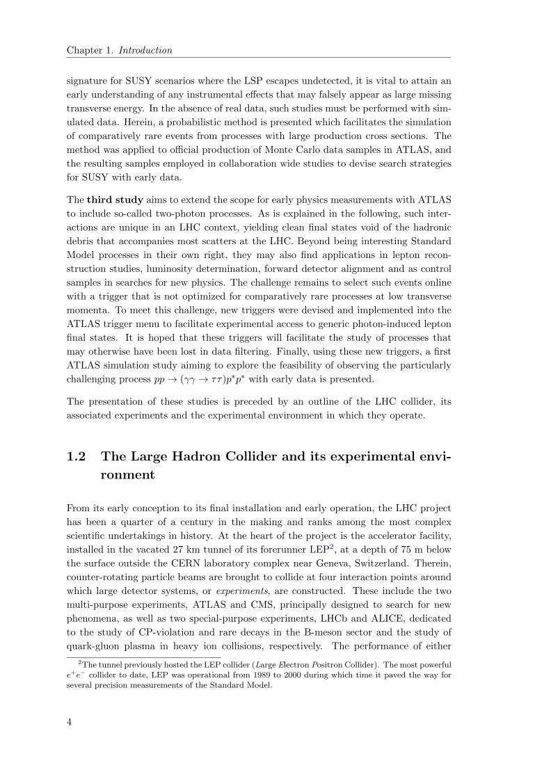
Chapter 1. Introduction
signature for SUSY scenarios where the LSP escapes undetected, it is vital to attain an
early understanding of any instrumental effects that may falsely appear as large missing
transverse energy. In the absence of real data, such studies must be performed with sim-
ulated data. Herein, a probabilistic method is presented which facilitates the simulation
of comparatively rare events from processes with large production cross sections. The
method was applied to official production of Monte Carlo data samples in ATLAS, and
the resulting samples employed in collaboration wide studies to devise search strategies
for SUSY with early data.
The third study aims to extend the scope for early physics measurements with ATLAS
to include so-called two-photon processes. As is explained in the following, such inter-
actions are unique in an LHC context, yielding clean final states void of the hadronic
debris that accompanies most scatters at the LHC. Beyond being interesting Standard
Model processes in their own right, they may also find applications in lepton recon-
struction studies, luminosity determination, forward detector alignment and as control
samples in searches for new physics. The challenge remains to select such events online
with a trigger that is not optimized for comparatively rare processes at low transverse
momenta. To meet this challenge, new triggers were devised and implemented into the
ATLAS trigger menu to facilitate experimental access to generic photon-induced lepton
final states. It is hoped that these triggers will facilitate the study of processes that
may otherwise have been lost in data filtering. Finally, using these new triggers, a first
ATLAS simulation study aiming to explore the feasibility of observing the particularly
challenging process pp→ (γγ → ττ)p∗p∗ with early data is presented.
The presentation of these studies is preceded by an outline of the LHC collider, its
associated experiments and the experimental environment in which they operate.
1.2 The Large Hadron Collider and its experimental envi-
ronment
From its early conception to its final installation and early operation, the LHC project
has been a quarter of a century in the making and ranks among the most complex
scientific undertakings in history. At the heart of the project is the accelerator facility,
installed in the vacated 27 km tunnel of its forerunner LEP2, at a depth of 75 m below
the surface outside the CERN laboratory complex near Geneva, Switzerland. Therein,
counter-rotating particle beams are brought to collide at four interaction points around
which large detector systems, or experiments, are constructed. These include the two
multi-purpose experiments, ATLAS and CMS, principally designed to search for new
phenomena, as well as two special-purpose experiments, LHCb and ALICE, dedicated
to the study of CP-violation and rare decays in the B-meson sector and the study of
quark-gluon plasma in heavy ion collisions, respectively. The performance of either
2The tunnel previously hosted the LEP collider (Large Electron Positron Collider). The most powerfule+e− collider to date, LEP was operational from 1989 to 2000 during which time it paved the way forseveral precision measurements of the Standard Model.
4

Chapter 1. Introduction
Figure 1.1: The CERN accelerator complex. [3]
experiment is contingent on the properties and configuration of the colliding beams
delivered by the LHC accelerator.
The following sections aim to highlight some of the key parameters governing the per-
formance of the LHC accelerator and to describe the characteristic features of the ex-
perimental environment it generates. A cursory overview of the central components of
the ATLAS detector is then given with a description of how they are designed to cope
with the challenges provided by the LHC environment.
1.2.1 The LHC machine
Having been constructed in the vacated LEP tunnel, the LHC profits greatly from
the existing beam injection infrastructure at CERN. The various components of the
accelerator chain are schematically depicted in Figure 1.1, and allow for a sequential
acceleration of the protons through a series of smaller machines:
• Initially, the protons are extracted from an ionized gas of hydrogen in a duoplas-
matron. After extraction, the protons are accelerated to 750 keV using quadrupole
radio frequency (RF) devices and then to a further 50 MeV in the LINAC2 linear
accelerator.
• The booster hikes the energy up to 1.4 GeV before injecting the protons into the
Proton Synchrotron (PS) in which they are grouped into packets of ∼ 1011 protons
5
Chapter 1. Introduction
0.1 1 1010
-7
10-6
10-5
10-4
10-3
10-2
10-1
100
101
102
103
104
105
106
107
108
109
10-7
10-6
10-5
10-4
10-3
10-2
10-1
100
101
102
103
104
105
106
107
108
109
σjet(E
T
jet > √s/4)
LHCTevatron
σt
σHiggs(M
H = 500 GeV)
σZ
σjet(E
T
jet > 100 GeV)
σHiggs(M
H = 150 GeV)
σW
σjet(E
T
jet > √s/20)
σb
σtot
proton - (anti)proton cross sections
σ (
nb)
√s (TeV)
even
ts/s
ec f
or L
= 1
033 c
m-2 s
-1
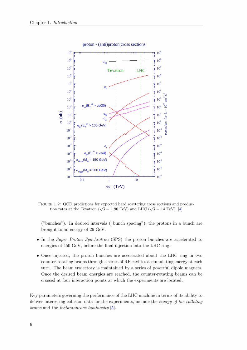
Figure 1.2: QCD predictions for expected hard scattering cross sections and produc-tion rates at the Tevatron (
√s = 1.96 TeV) and LHC (
√s = 14 TeV). [4]
(”bunches”). In desired intervals (”bunch spacing”), the protons in a bunch are
brought to an energy of 26 GeV.
• In the Super Proton Synchrotron (SPS) the proton bunches are accelerated to
energies of 450 GeV, before the final injection into the LHC ring.
• Once injected, the proton bunches are accelerated about the LHC ring in two
counter-rotating beams through a series of RF cavities accumulating energy at each
turn. The beam trajectory is maintained by a series of powerful dipole magnets.
Once the desired beam energies are reached, the counter-rotating beams can be
crossed at four interaction points at which the experiments are located.
Key parameters governing the performance of the LHC machine in terms of its ability to
deliver interesting collision data for the experiments, include the energy of the colliding
beams and the instantaneous luminosity [5].
6

Chapter 1. Introduction
As is further detailed in Section 1.3, the colliding protons are composite objects. A high
beam energy therefore ensures with non-negligible probabilty that collisions between
constituents carrying only a fraction of the total proton energy may still ensue at high
energy. An upper limit on the deliverable beam energy derives from the ability of the
magnet system to keep the beams in orbit along the required trajectory. In order to
deliver proton beams at the nominal energy of 7 TeV, the LHC relies on more than 1000
superconducting dipole magnets to produce the necessary 8.33 T magnetic field required
to bend the beam trajectory about the ring complex.
In order to ensure experimental sensitivity to rare processes, a high beam energy must
be accompanied by a sufficiently high collision rate. The instantaneous luminosity is a
machine parameter which quantifies the interaction rate per unit cross section:
L = νcollNANB
Aeff(1.1)
where NA,B quantify the number of particles in two incoming bunches A and B, brought
to collide in an effective area Aeff with frequency νcoll. As indicated by Equation 1.1,
the instantaneous luminosity can be amplified by increasing the collision frequency and
particle concentration in the colliding bunches, or by reducing the effective collision area.
In order to reduce the effective collision area, powerful quadropole magnets are employed
around the interaction points which serve to ”squeeze” the bunches from an incoming
beam spread of ∼ mm to a collisional beam spread of ∼ µm.
Increasing the number of particles in a bunch (”bunch intensity”), will also increase
the electromagnetic force field experienced by a particle in an opposing bunch. This
field is highly non-linear and may render the colliding beams unstable. Such beam-beam
interactions place an upper cap on the bunch intensity of ∼ 1011 protons per bunch [6].
Beam-beam interactions also limit the bunch concentration in the beamline. As the
number of bunches per beam increases, so does the probability of multiple bunch in-
teractions inside the detector volume3. In order to avoid additional unwanted head-on
beam collisions, a slight crossing angle Φ of O(∼ 100µrad) is introduced along the ex-
perimental insertions [5] which serve to reduce the occurrence of multiple short range
interactions between bunches inside the detector volume4.
Operating the LHC with a crossing angle comes at the cost of an increase in the effective
collision area and consequently a reduction in instantaneous luminosity. Translated into
beam parameters, Equation 1.1 may now be expressed as:
L = frevγNbn
2p
σxσyF (Φ, σx, σy) (1.2)
3The interaction regions all have ∼120 m straight sections were the counter-rotating beams arecontained in the same beam pipe. At the nominal bunch spacing of 7.5 m (25 ns), this correspondsto 120m
75m/2∼ 30 additional unwanted beam collisions per interaction region (in the absence of a crossing
angle).4Long range beam-beam interactions may still occur.
7

Chapter 1. Introduction
LHC TevatronCircumference (km) 26.7 6.3
Max. beam energy at collision (TeV) 7 1Beam energy at injection (TeV) 0.45 0.15
Dipole field at max. beam energy (T) 8.33 4.4Design luminosity (cm−2s−1) 1034 2.1× 1032
Bunch spacing (ns) 24.95 396Proton per bunch (1010) 11.5 27(p) / 7.5 (p)
Number of bunches 2808 36Total crossing angle (µrad) 285 0
Table 1.1: A comparison of main machine parameters at the LHC and Tevatron (RunII) [7, 8]
where frev is the beam revolution frequency, γ the relativistic Lorentz factor and Nb the
number of bunches each containing a total number of np protons. The effective collision
area is expressed in terms of the transverse RMS beam sizes σx,y at the interaction point
and is tempered by a geometric reduction factor F (Φ, σx, σy):
F (Φ, σx, σy) =1√
1 +(σzσ∗ tan Φ
2
)2 (1.3)
which depends on the crossing angle Φ and the ratio of longitudinal to transverse beam
profiles σz/σ∗.
When operating at design performance, the LHC will collide protons at center of mass
energies corresponding to√s =14 TeV with an instantaneous luminosity of 1034cm−2s−1
at crossing rate of 40 MHz. As such, LHC will significantly extend the sensitivity reach
to new physics beyond the current limits provided by the Tevatron collider. Table 1.1
provides a comparison of the main machine parameters of the LHC to those of the
Tevatron. Predicted cross sections and event rates for various processes are further
shown in Figure 1.2.
The LHC program also includes shorter periods of collision runs with heavy ions. Such
collision runs are not considered herein, but are given brief mention in Sections 1.3.4.1
and 4.7.
1.2.2 Early data prospects
The installation of the LHC commenced in 2000, during which time the LEP accelerator
was still operational. The assembly was completed in the autumn of 2007 and followed
by a period of commissioning during which the various sectors of the ring were gradually
cooled to an operating temperature of 1.9 K. On 10 September 2008, first beams where
successfully circulated in stages through the ring complex at the injection energy of 450
8

Chapter 1. Introduction
GeV. Several experiments along the ring collected splash5 events, thereby demonstrating
the operability of the detector apparatus.
On September 29 2008, during a powering test of the magnet circuits in Sector 3-46
of the LHC, a resistive zone developed in the (otherwise) superconducting electrical
weld between a dipole and a quadropole magnet. Following the local breakdown of
superconductivity, an electrical arc formed which punctured a liquid helium cooling
enclosure around a magnet, releasing helium into the insulating vacuum of the cryostat.
The subsequent pressure wave overwhelmed the escape relief valves, not only causing
the release of large amounts of helium from the magnet cooling system into the tunnel,
but also damaging and displacing several adjacent magnets [9]. The incident required
53 magnets to be removed from the tunnel and brought to the surface for cleaning and
repair, bringing the LHC to a temporary standstill and incurring a delay of one year.
In November 2009, operation briefly resumed at the injection energy (√s = 0.9 TeV )
in preparation for a longer physics run with 3.5 TeV beams. On 30 March 2010, the
first collisions at√s = 7 TeV were delivered to both ATLAS and CMS. At the time
of writing, it is foreseen that the LHC will continue to deliver√s = 7 TeV collisions
until ∼ 1fb−1 has been collected, before commencing a longer shutdown during which
the necessary preparations will be made for operation at the nominal beam energy of 7
TeV [10].
For reasons detailed in Section 1.3.6, the studies presented in Chapter 4 are very sensitive
to the evolution of the instantaneous luminosity. Table 1.2 provides some projective
estimates for the beam configurations and expected instantaneous luminosities for the
2010 run at√s = 7 TeV.
1.3 The phenomenology of proton-proton collisions
The potentially high center of mass energies achievable with a proton collider such as
the LHC comes at the price of exceedingly complex collisions. This complexity derives
in large part from the composite nature of the colliding protons and their strongly
interacting initial state. Because the hard collisions at the LHC take place between the
constituents of protons, the energy of the colliding quarks and gluons (partons) is not
equal to the center of mass energy√s of the incoming protons. By the same token, the
longitudinal component of the four-momenta of the colliding partons is a priori unknown.
The residual partons, which do not take part in the hard scatter, will typically carry the
larger fraction of the available energy. While most of this energy will disappear down
the beamline, a non-negligible fraction may still be scattered into the detector volume
thereby polluting the signatures of a potentially interesting event created in the hard
5”Splash events” ensue when a beam is made to collide with an upstream target outside the detector(rather than another colliding beam inside the detector), sending a ”splash” of secondary particles intothe detector volume.
6While the other seven sectors of the LHC had been fully commissioned to hold a beam energy of 5.5TeV prior to first beam injection on 10 September 2008, Sector 3-4 was the last sector to be commissionedand had not been powered to hold a beam of 5.5 TeV.
9
Chapter 1. Introduction
Phase Energy [TeV] Np (1010) Fill scheme β∗ [m] L [cm−2s−1]Beam commissioning, safebeam limit
3.5 2 2× 2 11 2.6× 1027
Beam commissioning, safebeam limit, squeeze
3.5 2 2× 2∗ 2 3.6× 1028
Bunch trains from SPS 3.5 3 43× 43 2 1.7× 1030
Increase intensity3.5 5 43× 43 2 4.8× 1030
3.5 5 156× 156 2 1.7× 1031
3.5 7 156× 156 2 3.4× 1031
Introduce crossing angle,truncated 50 ns
3.5 7 50ns - 144∗∗ 2.5 2.5× 1031
Increase intensity3.5 5 50ns - 288 2.5 2.6× 1031
3.5 7 50ns - 432 2.5 7.5× 1031
3.5 7 50ns - 796 2.5 1.4× 1032
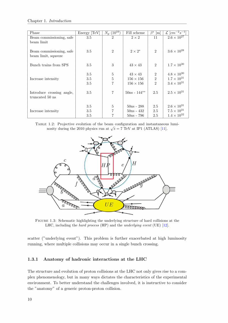
Table 1.2: Projective evolution of the beam configuration and instantaneous lumi-nosity during the 2010 physics run at
√s = 7 TeV at IP1 (ATLAS) [11].
Figure 1.3: Schematic highlighting the underlying structure of hard collisions at theLHC, including the hard process (HP) and the underlying event (UE) [12].
scatter (”underlying event”). This problem is further exacerbated at high luminosity
running, where multiple collisions may occur in a single bunch crossing.
1.3.1 Anatomy of hadronic interactions at the LHC
The structure and evolution of proton collisions at the LHC not only gives rise to a com-
plex phenomenology, but in many ways dictates the characteristics of the experimental
environment. To better understand the challenges involved, it is instructive to consider
the ”anatomy” of a generic proton-proton collision.
10
Chapter 1. Introduction
Figure 1.3 provides a schematic depiction of the evolution of a typical interaction between
two incoming protons. Three lines are seen to eminate from either proton, signifying
the valence quark constituents. These ”quark-lines” are seen to interact by way of gluon
exchanges (curly lines).
If the momentum exchange between the constituents of the either proton is sufficiently
large, a hard scattering event may ensue, whereby the interacting partons are ”expelled”
from proton confinement and act as quasi-free agents. Such a hard scattering is depicted
at the top of Figure 1.3. The final state resulting from the hard interaction will depend on
the energy available to the interacting partons and their respective quantum numbers.
In rare cases, such interactions may result in the production of heavy particles, such
as Z/W bosons or potentially even new physics. The hard process depicted in Figure
1.3 however, counts among the most prolific interactions at the LHC and constitutes a
formidable background to all studies presented herein. The two incoming partons, here
a quark and a gluon, interact to produce another quark-gluon pair. The outgoing quark
and gluon will both continue to radiate until their energies fall below a critical threshold
after which they can no longer be considered quasi-free and will be forced to hadronize
into colour neutral bound states known as mesons and baryons. If these bound states
are excited, they will in turn decay into relatively long-lived observable particles such as
pions, kaons, protons and neutrons. Such a spray of hadronic debris is known as a jet,
and the mean direction of the jet constituents is expected to follow along the direction of
the instigating quark or gluon. Because the jet constituents are colour neutral objects,
whereas the quarks and gluons are not, there is necessarily a colour connection between
the outgoing partons. Consequently the spatial region between the two jets is likely
to be ”polluted” by low energy hadronic debris. The implications for the experimental
detector systems are profound, in the sense that even a simple di-jet event as depicted
in Figure 1.3 may be expected to render final states with a large number of (low energy)
particles scattered across the entire central detector volume.
With the hard scattered parton pair ejected from either proton, the proton remnants
are left in an unstable colour charged state, still colour connected to the hard sub-
process. The proton remains interact primarily via soft scattering processes involving
comparatively small momentum transfers. Unlike the products of the hard scattering,
the resulting hadronic debris is therefore typically scattered at small angles with re-
spect to the direction of the colliding protons7. The Underlying Event (UE) comprises
everything that accompanies a proton-proton interaction apart from the hard scatter,
and serves to further complicate the experimental conditions at the LHC. Not only does
the large flux of forward scattered debris put stringent demands on forward detector
systems, but the colour connection to the hard subprocess, exemplified in Figure 1.3
through e.g. gluon emission d, will often result in particle production in the central
detector regions overlapping with the signatures of the hard scatter.
The experimental challenges resulting from the complexity of proton-proton interactions,
are further exacerbated by the high multiplicity of protons involved in a single bunch
crossing interaction. As mentioned in Section 1.2.1, protons are not brought to collide
7Semi-hard or secondary hard-scatterings may also occur between proton remnant constituents.
11

Chapter 1. Introduction
individually, but rather in packets (”bunches”) of 1011 protons. The proton-proton
interaction depicted in Figure 1.3 is therefore just one of many interactions taking place
between protons in a crossing. While it is unlikely for a single bunch crossing to contain
more than one hard scattering event, soft scattering processes between other protons
in a bunch are commonplace. Such interactions are dubbed minimum bias (or pile-up
when overlapping with a hard scatter) and are given further mention in Section 1.3.6.
In summary therefore, the key signatures of nearly all interesting scattering events at
the LHC are likely to be overlaid with debris from initial and final state radiation, the
underlying event created by the beam remnants as well as soft scatters from other proton
pairs in the same bunch crossing. The experimental challenge is in part to disentan-
gle the signatures of the hard process under investigation from those of accompanying
underlying processes.
In the following, some of the key issues in the phenomenological description of hadronic
interactions at the LHC are briefly highlighted.
1.3.2 The hard interaction
At the energies accessible to the LHC, each proton in a bunch crossing may be regarded
as a ”gas” of quasi-free partons, each carrying a certain momentum fraction xp of the
total proton momentum. As shown in Figure 1.3, the partonic constituents of two collid-
ing protons may interact in different ways and the nature of the interaction will depend
on the momentum transfer Q2 involved. Most processes of interest are relatively rare
occurrences and involve mass scales far in excess of the proton mass, such as e.g. Z or
top production. Such processes only follow from large Q2 exchanges and are dubbed
hard scattering processes because the interacting partons both carry a significant pro-
ton momentum fraction xp. Unlike soft scattering processes (low Q2), hard scattering
processes can be described with perturbative QCD within the framework of the parton
model.
In general terms, perturbation theory allows one to express the cross section as an
expansion in the strong coupling constant αS8:
σ ∼ αmS∞∑n=0
cnαnS (1.4)
where the exponent m depends on the process under consideration and the coefficients
cn are functions of the momenta of the incoming and outgoing partons. An exact
calculation to all orders in the expansion in Equation 1.4 is currently impossible and
calls for a focus on the terms that provide the most significant corrections. While
leading order (n=0) calculations are readily available for most processes expected to
occur at the LHC, calculations one and two orders beyond are more scarce. In any
8Assuming electroweak contributions are small compared to contributions from QCD.
12

Chapter 1. Introduction
Figure 1.4: Generic 2→ N hard scattering process at the LHC.
event, a truncation of the perturbation series is required and in so doing one necessarily
introduces a dependence on the renormalization scale µ2R
9[13]:
σ ∼ σLO + αS(µ2R)σNLO + ...+ αkS(µ2
R)σNkLO. (1.5)
The cross section σ quantifies the probability of a transition from an initial incoming
state in to a final outgoing state out. Using the Lagrangian of the underlying theory, it
is possible to express this probability in terms of the invariant matrix element M for
the process under inspection and the momenta of the incoming and outgoing partons
involved:
Pin→out = |< out|iT |in >|2 =∣∣∣(2π)4δ4
(∑pin −
∑pout
)iM(pin → pout)
∣∣∣2 (1.6)
where the transition matrix T is defined in terms of the scattering matrix S = 1 + iT
[14]. For the 2→ n process depicted in Figure 1.4, this partonic cross section may take
on the general differential form:
dσ2→n =1
4Ep1Ep2
1∏k nk!
|T |2n∏i
d3qi(2π)32Eqi
(2π)4δ4(p1 + p2 −n∑i
qi) (1.7)
where Ep(Eq) is the energy of the incoming (outgoing) particles and ni the number of
identical particles of type k in the scattered final state [15].
At a hadron collider such as the LHC, the partonic cross section as given by Equation
1.7 is not directly measurable, the reason being that the initial state partons are con-
stituents of colliding protons with a priori unknown momenta. In order to compute the
measurable hadronic cross section, it is necessary to fold in the probability of extracting
a parton of a particular flavour a carrying a momentum fraction xa from an incom-
ing hadron A. This information is encoded into so-called Parton Distribution Functions
9If the calculation were to be carried out to all orders, the dependence on µ2R would vanish, but since
each term in the expansion separately depends on it any fixed order will necessarily depend on the choiceof µ2
R. In principle, the choice of µ2R is arbitrary, however in order to avoid contributions of the sort(
αS(µ2Rln
(QµR
)))n
from the nth term in the expansion to grow large and compromise the robustness
of the fixed order calculation, the renormalization scale is typically placed in the vicinity of the hardscattering scale Q2.
13

Chapter 1. Introduction
(PDF) fa/A(xa, µ2F ), which in turn depend on the energy scale µ2
F at which the incom-
ing hadrons are probed. The energy scale µ2F is also dubbed the factorization scale,
as it marks the separation of perturbative short distance physics from non-perturbative
long-distance physics. Figure 1.3 shows one of the partons participating in the hard
interaction radiating a gluon before interacting with a parton from the opposite hadron.
The probability of such a collinear emission grows logarithmically with the inverse of
the momentum of the emitted gluon and thus potentially blights the convergence of the
perturbative expansion in Equation 1.5. However, by way of the so called DGLAP evolu-
tion equations [16–18], these large logarithms can be absorbed into the PDFs. Aided by
factorization theorems [19], the observable hadronic cross section can now be expressed
as a convolution of the PDFs with the partonic cross section dσ:
dσpApB =∑a,b
∫ 1
0dxa
∫ 1
0dxbfa/A(xa, µ2
F )fb/B(xb, µ2F )dσa+b→X(µ2
R) (1.8)
The numerical prediction will depend on the arbitrary choice made for the two unphysical
scales µ2R and µ2
F10. This dependence mirrors the uncertainty introduced by neglecting
higher order corrections. The total cross section of a process at the LHC is therefore seen
to be a combination of both perturbative and non-perturbative contributions, the latter
of which are absorbed by the PDFs. These non-perturbative effects imply that PDFs
cannot be derived from theory, but must be extracted from experimental measurements.
The PDFs on which most predictions for the LHC are based are derived from extrapo-
lations of such measurements performed primarily at the lower-energy colliders HERA
and Tevatron, thereby introducing another source of uncertainty into the predictions.
1.3.3 From hard scattering to experimental observables
At the LHC, the outgoing partons will tend to emerge from the hard scattering at
comparatively high energies so that initially they may still be regarded as quasi-free
agents. As such, they will radiate and lose energy until they are soft enough to hadronize
into colour neutral states.
1.3.3.1 Parton showers
The radiation process associated with the final state partons may be described by higher
order terms in the expansion of Equation 1.5, or if such corrections are unavailable by
way of phenomenological models. Such models are commonly dubbed parton showering
models. Parton showering algorithms take all outgoing partons of a LO matrix element
calculation and allow each parton to branch out into a multi-parton final state through
successive splittings of the form a→ b+ c, as shown in Figure 1.5. Each daughter may
branch in turn to form a sequence of consecutive splittings.
10Conventionally these scales are chosen close to the momentum scale of the hard scatter.
14
Chapter 1. Introduction
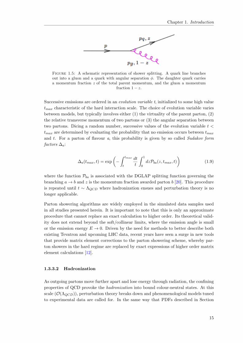
Figure 1.5: A schematic representation of shower splitting. A quark line branchesout into a gluon and a quark with angular separation φ. The daughter quark carriesa momentum fraction z of the total parent momentum, and the gluon a momentum
fraction 1− z.
Successive emissions are ordered in an evolution variable t, initialized to some high value
tmax characteristic of the hard interaction scale. The choice of evolution variable varies
between models, but typically involves either (1) the virtuality of the parent parton, (2)
the relative transverse momentum of two partons or (3) the angular separation between
two partons. Dicing a random number, successive values of the evolution variable t <
tmax are determined by evaluating the probability that no emission occurs between tmaxand t. For a parton of flavour a, this probability is given by so called Sudakov form
factors ∆a:
∆a(tmax, t) = exp
(−∫ tmax
t
dt
t
∫ 1
0dzPba(z, tmax, t)
)(1.9)
where the function Pba is associated with the DGLAP splitting function governing the
branching a→ b and z is the momentum fraction awarded parton b [20]. This procedure
is repeated until t ∼ ΛQCD where hadronization ensues and perturbation theory is no
longer applicable.
Parton showering algorithms are widely employed in the simulated data samples used
in all studies presented herein. It is important to note that this is only an approximate
procedure that cannot replace an exact calculation to higher order. Its theoretical valid-
ity does not extend beyond the soft/collinear limits, where the emission angle is small
or the emission energy E → 0. Driven by the need for methods to better describe both
existing Tevatron and upcoming LHC data, recent years have seen a surge in new tools
that provide matrix element corrections to the parton showering scheme, whereby par-
ton showers in the hard regime are replaced by exact expressions of higher order matrix
element calculations [12].
1.3.3.2 Hadronization
As outgoing partons move further apart and lose energy through radiation, the confining
properties of QCD provoke the hadronization into bound colour-neutral states. At this
scale (O(ΛQCD)), perturbation theory breaks down and phenomenological models tuned
to experimental data are called for. In the same way that PDFs described in Section
15

Chapter 1. Introduction
(a) The string fragmentation model (b) The cluster fragmentation model
Figure 1.6: Schematic representation of hadronization models [21].
1.7 associate the incoming partons of the hard scattering with incoming hadrons, frag-
mentation functions of the form Hp→h(z, µhF ) provide a mapping between ”free partons”
and bound hadrons. These functions encode the probability that a parton of flavour p
hadronizes into a hadron of type h, in the process of which it loses a momentum fraction
z. Like the PDFs, such fragmentation functions are sensitive to the factorization scale
µhF which separates the perturbative partonic physics from the non-perturbative effects
absorbed by the fragmentation functions. Fragmentation functions are employed in var-
ious hadronization models, whose common underlying assumption is that the parton
concentration in a region of the detector before hadronization is reflected in the quark
constituents of hadrons in that same region after hadronization [12].
Two widely used models include the Lund string model [22] and the Cluster model [23],
schematically depicted in Figure 1.6.
The former connects quarks and antiquarks via a linearly increasing colour field rep-
resented by a string. Gluons appear as kinks along this string. As the qq-pair moves
apart, the potential energy in the string increases until it sufficiently large to produce a
qq-pair, after which the string splits in two as prescribed by the fragmentation functions.
This procedure is iterated until all energy is bound up in hadrons.
The cluster model by contrast, initially splits all gluons into qq-pairs and then attempts
to gather all qq-pairs in the event into colour singlets. These resulting clusters are then
subsequently decayed into a pair of hadrons.
After hadronization, any unstable hadrons decay into long-lived particles such as K±,
K0, p, n, π±, π0, γ, etc. Along with any long lived particles produced in the hard inter-
action, these particles then make up the experimental observables of the hard scattering.
Properly tuned, both models (and variants thereof) have been found to render final
states in good agreement with data [12]. The availability of accurate hadronization
models is essential for the development of experimental tools that rely on the ”global”
and constituent properties of jets, such as the studies presented in Chapter 2.
16
Chapter 1. Introduction
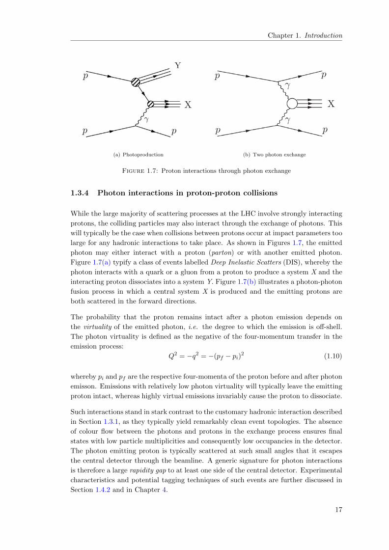
(a) Photoproduction (b) Two photon exchange
Figure 1.7: Proton interactions through photon exchange
1.3.4 Photon interactions in proton-proton collisions
While the large majority of scattering processes at the LHC involve strongly interacting
protons, the colliding particles may also interact through the exchange of photons. This
will typically be the case when collisions between protons occur at impact parameters too
large for any hadronic interactions to take place. As shown in Figures 1.7, the emitted
photon may either interact with a proton (parton) or with another emitted photon.
Figure 1.7(a) typify a class of events labelled Deep Inelastic Scatters (DIS), whereby the
photon interacts with a quark or a gluon from a proton to produce a system X and the
interacting proton dissociates into a system Y. Figure 1.7(b) illustrates a photon-photon
fusion process in which a central system X is produced and the emitting protons are
both scattered in the forward directions.
The probability that the proton remains intact after a photon emission depends on
the virtuality of the emitted photon, i.e. the degree to which the emission is off-shell.
The photon virtuality is defined as the negative of the four-momentum transfer in the
emission process:
Q2 = −q2 = −(pf − pi)2 (1.10)
whereby pi and pf are the respective four-momenta of the proton before and after photon
emisson. Emissions with relatively low photon virtuality will typically leave the emitting
proton intact, whereas highly virtual emissions invariably cause the proton to dissociate.
Such interactions stand in stark contrast to the customary hadronic interaction described
in Section 1.3.1, as they typically yield remarkably clean event topologies. The absence
of colour flow between the photons and protons in the exchange process ensures final
states with low particle multiplicities and consequently low occupancies in the detector.
The photon emitting proton is typically scattered at such small angles that it escapes
the central detector through the beamline. A generic signature for photon interactions
is therefore a large rapidity gap to at least one side of the central detector. Experimental
characteristics and potential tagging techniques of such events are further discussed in
Section 1.4.2 and in Chapter 4.
17
Chapter 1. Introduction
In the following, the theoretical considerations underpinning photon interactions at the
LHC are briefly expounded.
1.3.4.1 Theoretical description of photon interactions at hadron colliders
Photon emissions from an incoming beam of hadrons are often described by means of
the Equivalent Photon Approximation (EPA) [24].
EPA regards the electromagnetic fields of the incoming hadrons as comparable to a flux
of photons with spectra dN(ω,Q2), whereby ω =EγE is the fraction of the incoming
hadron energy associated with this photon flux and Q2 the virtuality of the photon
emission.
By a procedure reminiscent of the factorization employed in the treatment of hadronic
interactions in Section 1.3.2, the scattering amplitude for emissions with low photon
virtuality may be separated into a (long distance) flux dependent function and the (short
distance) cross section of the relevant γp or γγ interaction process. The differential cross
sections for the scatters depicted in Figures 1.7(a) and 1.7(b) may then be expressed as
a convolution of the photon interaction cross section and the photon flux spectra [25]:
dσγp = σγp→XdN(ω,Q2) (1.11)
dσγγ = σγγ→XdN(ω1, Q21)dN(ω2, Q
22) (1.12)
In this fashion, the dependence on the photon virtuality is moved from the photon
interaction cross sections σγp→X and σγγ→X to the photon flux dN . If the photon cross
sections are relatively insensitive to the photon virtuality, the integrated interaction cross
sections for the photoproduction process depicted in Figure 1.7(a) may be expressed in
terms of the luminosity function fγ :
σpp(γp→X)pY (s) =
∫ 1
ωmin
fγσγp→X(ω, s)dω (1.13)
whereby fγ is the Q2-integrated photon flux, restrained by kinematics or experimental
constraints:
fγ =
∫ Q2max
Q2min
dN(ω,Q2)dQ2 (1.14)
and s the square center of mass energy of the colliding hadron beams.
In a similar manner, the integrated interaction cross section for the two photon process
depicted in Figure 1.7(b) may be expressed as:
σpp(γγ→X)pp(s) =
∫ √sWmin
dWγγdLγγdWγγ
(W, s)σγγ→X(W ) (1.15)
18
Chapter 1. Introduction
where the relative luminosity function is defined in terms of the invariant mass Wγγ of
the outgoing system X and comprises the integrated flux of both photons:
dLγγdWγγ
=
∫ 1
W 2γγ/s
2Wγγfγ(ω)fγ
(W 2γγ
ωs
)dω
ωs(1.16)
The EPA factorization scheme treats the exchanged photons as quasi-real (unpolarized)
particles, and its validity is restricted to exchanges where the interaction cross section
of the σγp(γ) may be considered insensitive to the photon virtuality Q2, that is to say
Q2 < Λγ , where Λγ represents some dynamical cut-off scale [24]. For colliding protons
at the LHC, this cut-off is provided for by the proton electromagnetic form factors.
These form factors reflect the internal electromagnetic structure of composite colliding
hadrons and ensure that σγp(γ) rapidly falls when Q2 > Λγ [25, 26]. It is notable
that photon-induced interactions typically take place at impact parameters b ∼ 1/√Q2
much larger than the strong interaction range [25] and may therefore be considered
largely insensitive to the internal structure of the colliding species. As such, one can
also expect photon interactions to characterize so called ultraperipheral collisions between
heavy ions, whereby nuclei of charge Z interact electromagnetically at impact parameters
greater than the nuclear radii11 [27]. The field intensity associated with the colliding
species is then enhanced by a factor Z2, so that the two-photon interaction rate is
expected to intensify considerably:
σHI(γγ → X)
σpp(γγ → X)∼ Z4. (1.17)
Figure 1.8 compares the effective two-photon luminosities as a function of the invariant
mass of the central system Wγγ for various colliding species at the LHC and LEPII. The
LHC is seen to have both energy and luminosity reach well beyond LEPII, a feature
which in recent years has sparked new interest in regarding the LHC as a partial photon
collider. While photon-induced processes have been extensively studied at both LEP and
HERA, the LHC presents the first opportunity to study photon-induced center of mass
energies beyond the electroweak scale [29]. By integrating the luminosity spectrumdLγγdWγγ
,
the fraction of the total LHC proton-proton luminosity available for Wγγ > 23 GeV and
Wγγ > 225 GeV scatters has been estimated to be 1% and 0.1%, respectively. In light
of the comparatively large luminosity available at the LHC, these numbers indicate that
even comparatively scarce two-photon processes may have detectable rates [25].
These features combined invite for a range of different studies, both within and beyond
the Standard Model, the latter partially exemplified by the diagrams in Figure 1.9. A
more detailed discussion of the potential physics programme with two-photon processes
at the LHC can be found in [25, 29].
The observation of the process γγ → l±l∓ with early LHC data is the focus of Chapter
4, and further discussions of topics relevant to the experimental detection of two-photon
processes can be found therein.
11This condition partially protects against the occurrence of simultaneous hard interactions.
19

Chapter 1. Introduction
Figure 1.8: The effective γγ luminosity as a function of Wγγ for various collidingspecies at the LHC (
√s = 14 GeV) compared to LEP (
√s = 200 GeV). In either case
effective luminosity is measured against a total luminosity scenario corresponding to ∼1 collision per bunch crossing [28].
(a) Higgs (b) SUSY
Figure 1.9: New physics beyond the Standard Model in two-photon interactions: (a)Higgs production (b) SUSY slepton production, whereby each slepton decays into a
chargino and a lepton.
1.3.5 The underlying event
The previous sections were primarily concerned with the phenomenology connected to
the treatment of the primary interaction, be it the hard scattering between two proton
constituents or the exchange of photons between protons.
Only in rare cases, does a primary interaction occur without the participating proton
”breaking up”, and the remnants following such a dissociation will interact and fragment
to produce the underlying event.
The physics of the underlying event is non-perturbative and comparatively poorly un-
derstood, but the experimental implications will typically depend on how decoupled the
primary interaction is from the proton fragmentation.
20

Chapter 1. Introduction
In the absence of a colour connection to the primary interaction, the fragmentation
products are most likely to scatter at small angles with respect to the parent proton
directions. With a transverse component premn.T premn.z , it is reasonable to expect the
elements of the underlying event to escape undetected down the beamline. This scenario
is typically realized in photon interactions as described in Sections 1.3.4 and 4.2.
Primary interactions involving partons extracted from the interacting protons, however,
typically leave the proton remnants in a colour charged and unstable state. In such
cases, the remnants can only ”neutralize” through soft (long-distance) interactions with
the partons involved in the primary interaction. As a consequence, the proton frag-
ments may be scattered beyond the very forward directions and into the central rapidity
regions. From an experimental standing, the underlying event in such cases pollutes
the signatures of the primary interaction and complicates the analysis of the data. The
underlying event is in no small part responsible for the high multiplicity final states
expected to follow from hadronic interactions at the LHC, and the presence of a large
number of additional particles without relation to the primary interaction, can be ex-
pected to confuse and degrade the performance of offline reconstruction algorithms such
as those described in Chapter 2.
While the structure of the underlying event counts among the least understood aspects
of the hadronic environment at the LHC, there are strong indications that so-called
multiple parton interactions of semi-hard nature play a key role. Such scatters were first
established in γ + 3 jet events at CDF, identified as the overlap of a separate γ+jet
process and a jet+jet process within the same pp interaction [30]. The result implicates
a considerable probability for partons in the proton remnants to independently undergo
secondary (semi-hard) interactions alongside the primary interaction. Hard scattering
interactions typically occur in collisions involving a small impact parameter, hence the
harder the primary interaction, the more likely it is that it will be accompanied by
secondary partonic interactions. By the same token, multiple interactions are unlikely
to occur in photon-exchange processes.
There are, however, also indications that multiple scattering cannot describe the full
structure of the underlying event and that an additional highly non-perturbative soft
component must be accounted for [12]. In summary therefore, a single strongly interact-
ing proton-proton collision should be regarded as an overlap between the primary hard
interaction, any secondary semi-hard interactions and residual soft-interactions of the
colour-charged remnants.
Several phenomenological models exist which in various ways attempt to predict the
structure of the underlying event. These models are all tuned to experimental measure-
ments performed at previous collider experiments with various degrees of success. There
is therefore still considerable uncertainty connected to the validity of these tunings when
extrapolated to LHC energies [12].
21

Chapter 1. Introduction
1.3.6 Pile-up and Minimum Bias
As already alluded to in Section 1.3.1, the protons are not brought to collide individually,
but in bunches of high proton density. A high proton density not only increases the
chances of a hard interaction to take place, but equally the probability of simultaneous
soft interactions between other protons in the same bunch crossing. Interactions in
a bunch crossing between proton pairs with no relation to the hard scatter are often
referred to as pile-up 12. Pile-up interactions further complicate the interpretation of
data, and are particularly detrimental to the selection of photon-induced final states, as
is further discussed in Section 4.2.
In general, the number of independent interactions N taking place in a single bunch
crossing will follow a Poisson distribution
P (N ; νN ) = νNNe−νN
N !(1.18)
whose mean value νN = σppL〈∆tbunch〉 will depend on the instantaneous luminosity Land the bunch spacing
〈∆tbunch〉 =1
40MHz× NBNmaxB
(1.19)
given by the ratio of bunches per beam NB to the maximal number of bunch slots
available13 [31].
L[cm2s−1] Np / bunch Fill scheme (NB ×NB) νN (σND+DD)
7.0× 1027 2× 10¹⁰ 2× 2 0.021.7× 1030 3× 10¹⁰ 43× 43 0.224.8× 1030 5× 10¹⁰ 43× 43 0.621.7× 1031 5× 10¹⁰ 156× 156 0.603.4× 1031 7× 10¹⁰ 156× 156 1.209.4× 1031 7× 10¹⁰ 432× 432 1.201.8× 1032 7× 10¹⁰ 796× 796 1.25
1.0× 1033 — 2808× 2808 2.201.0× 1034 1.15× 10¹¹ 2808× 2808 21.89
Table 1.3: The estimated mean pile-up νN for various early luminosity scenariossketched in Table 1.2 assuming
√s =7 TeV and σND+DD ∼62 mb. The two bottom
rows assumes√s =14 TeV and σND+DD ∼69 mb.
Table 1.3 lists the average expected pile-up at various luminosities and beam configu-
rations at the LHC. It is notable that a rise in luminosity following an increase in the
number of protons per bunch crossing results in more pile-up than does a luminosity rise
12The term pile-up is often also used to denote the overlap between signals from two consecutive bunchcrossings in the detector. Such overlaps may follow whenever the response time of a detector subsystemexceeds the bunch spacing of the colliding beam.
13At the LHC, NmaxB = 3564.
22

Chapter 1. Introduction
Cross section (mb)Process PYTHIA PHOJET
σtot 102 (91) 120 (106)σel 23 (19) 35 (29)σinel 79 (72) 85 (76)
σND 55 (49) 68 (62)σSD 14 (14) 11 (11)σDD 10 (9) 4 (4)σCD N/A 1 (N/A)
Table 1.4: Relative composition of the total proton-proton cross section at the LHCas predicted by the Monte Carlo generators PYTHIA and PHOJET for
√s =14 TeV
(7 TeV). The discrepancies reflect the uncertainties when extrapolating existing modeltunings to LHC energies. The lower section breaks down the contributions to the
inelastic cross section σinel [32, 33].
Figure 1.10: Various soft elastic and inelastic scattering processes, with correspondingevent topologies in η−φ space, whereby coloured regions indicate particle activity and
empty regions rapidity gaps [34].
following an increase in the number of bunches. Table 1.3 also indicates that whereas
additional pile-up events are comparatively scarce at low luminosity, an average of 22
pile-up events are expected to accompany every hard scatter at design luminosity.
To understand the nature of these additional pile-up interactions, it is instructive to
consider the dominant components of the total proton-proton scattering cross section
at the LHC. This cross section may be expressed as a sum of its elastic (σel) and
inelastic (σinel) contributions, where σel < σinel. The large majority of interactions in
a bunch crossing, and consequently most additional pile-up interactions, are therefore
likely to be soft, inelastic (non-perturbative) scatters. Such scatters are often dubbed
minimum bias interactions in reflection of their experimental collection under minimal
trigger conditions [32], however a distinction is often drawn between diffractive and non-
diffractive contributions. The diffractive contribution may in turn be subdivided into
single-diffractive (SD), double-diffractive (DD) and central-diffractive (CD) components,
as shown in Figure 1.10. Table 1.4 compares the relative contributions of such inelastic
subprocesses and indicates that the total proton-proton cross section:
σpptot = σelastic + (σND + σSC + σDD + σCD) (1.20)
23

Chapter 1. Introduction
Figure 1.11: Cumulative luminosity versus day delivered by the LHC (green) andrecorded by ATLAS (yellow) during stable beams at
√s = 7 TeV. (The systematic
uncertainty associated with the luminosity measurement is estimated at 11%).
is dominated by non-diffractive (ND) inelastic scatters. Non-diffractive inelastic inter-
actions are characterized by proton fragmentation through gluon emission into colour
neutral bound states, whereby the hadronic debris is scattered into both forward and
central rapidity regions [35]. While the scattered objects are typically very soft, collisions
involving an overlap between a photon-induced process and a non-diffractive scatter is
likely to render the former non-exclusive.
Diffractive scatters by contrast involve colour-neutral (”pomeron”) exchanges between
the interacting protons, as depicted in Figure 1.10. Common to all diffractive scatters is
the presence of large rapdidity gaps, which follow from the absence of a colour connection
between the scattered protons or between the scattered protons and the central system.
Diffractive processes therefore share many experimental similarities with two-photon
processes and may be falsely identified as such. Diffraction as a potential background
to two-photon processes is further discussed in Chapter 4.
1.4 The ATLAS experiment
The ATLAS14 experiment counts among the largest scientific collaborations to date,
involving almost 3000 scientists and engineers from across 37 different countries15. For-
mally proposed in 1994 [36], the construction and assembly of the experimental appara-
tus was largely completed in 2008. At the time of writing, the detector is (almost) fully
operational and has recorded a total of ∼ 300nb−1 of data, as shown in Figure 1.11.
The physics programme of the ATLAS experiment is akin to that of CMS, including
both improvements to current Standard Model measurements and extensive searches for
new physics beyond. This ambitious programme coupled with the harsh experimental
environment of the LHC, have driven the design and technology choices of the ATLAS
14A Toroidal LHC ApparatuS15As of December 2009.
24

Chapter 1. Introduction
Figure 1.12: Cut-away view of the ATLAS central detector with its component sub-detectors [37].
detector. A detailed description of the experimental programme and the various detec-
tor components can be found in [32] and [37]. In the following a cursory overview of
the various detector systems of the ATLAS experiment is given, with a light emphasis
on components of particular relevance to the studies presented herein. The ATLAS
coordinate system and relevant associated quantities are summarized in Appendix A.
1.4.1 The central detector systems
Following the general design principles of a typical multi-purpose detector, the cen-
tral detector system is centered around the interaction region and consists of several
specialized subdetectors arranged in layers about the beamline in an approximately φ-
symmetric fashion. The cylindral volume of any component subdetector is characterized
by a coaxial barrel flanked by perpendicularly arranged end-caps to either side.
Stable and quasi-stable particles emerging from the interaction region will extend into the
detector volume and interact with the material therein, whereby the mode of interaction
will depend on the properties of the traversing particle and the material through which
it is passing. The detection technologies employed in each detector layer are therefore
designed to exploit particular forms of particle interactions with matter to render partial
information towards the energy and direction of outgoing particles. As discussed in
Chapter 2, a full-fledged measurement of the properties of a given particle along with an
identification of its type is an involved procedure that typically relies on the combined
information provided by several subdetectors.
25

Chapter 1. Introduction
The composition of the ATLAS central detector is depicted in Figure 1.12. The inner
detector forms the innermost detector subsystem, whose primary task is to measure
the flight paths (”tracks”) of charged particles. Surrounding the inner detector is the
calorimetry, designed to measure particle energies. The outermost detector system com-
prises the various chambers of the muon spectrometer, designed to measure the momenta
of charged minimum ionizing particles16 whose energies are not fully absorbed in the
calorimeters. With total dimensions of 44m × 25m and a weight of 7000 tonnes, the
ATLAS detector is the largest particle physics detector to date.
1.4.1.1 The innermost tracking detectors
The inner detector (ID) comprises the three innermost detector subsystems and is de-
signed to provide accurate measurements of the direction, momentum and impact pa-
rameters17 of charged particles. Using pattern recognition techniques, this information
can be exploited to reconstruct the tracks of charged particles as well as any vertices
from which several tracks emerge [32]. Their close proximity to the interaction region
render the inner tracking detectors particularly exposed to high particle densities and
associated radiation levels. At design luminosity, it is expected that roughly 103 ionizing
particles will be scattered into the ID volume with every bunch crossing. In order to
retain the best possible momentum and vertex resolutions in this environment, tech-
nologies offering differing levels of granularity are employed at increasing radii from the
beamline. The various subsystems of the ID volume are shown in Figure 1.13.
The two innermost subdetectors employ silicon based technologies to provide high res-
olution measurements where the particle densities are at their highest. When ionizing
particles pass through the sensitive semi-conductor material, electron-hole pairs are re-
leased along their flight path and collected by an electric field created by an externally
applied bias voltage [39].
The Pixel Detector
The high particle flux environment in the immediate vicinity of the beampipe mandates
the use of pixel technology to obtain the required granularity to secure high resolution
measurements. The three innermost layers therefore constitute the Pixel Detector, which
with its roughly 80 million pixels of size (R − φ) × z = 50 × 400µm2 is capable of
delivering spatial resolutions of 10 µm in (R − φ) and 115 µm in z (barrel) 18. The
first layer, often called the vertexing layer or b-layer, is located at a radial distance of
only 51mm from the beamline. The close proximity to the interaction region allows for
an accurate determination of the primary vertex and the identification of any displaced
vertices, but at the same time exposes the detector hardware to very large radiation
16A minimum ionizing particle (MIP) is a particle whose mean energy loss through matter is close tothe minimum [38].
17The impact parameter measures the distance of closest approach in space between a track and theprimary vertex.
18The resolution is not only limited by the pixel size, but also by any material in front of the sensormaterial, the angle of incidence, the readout technology, etc.
26

Chapter 1. Introduction
(a) Cut-away view of the ATLAS inner detector volume
(b) Schematic illustrating the passage of a pT ∼10 GeV charged particle (red line)through the various layers of the inner detector volume.
Figure 1.13: The ATLAS inner detector [37].
27
Chapter 1. Introduction
doses. Consequently it is forseen that the vertexing layer will require replacement after
three years of nominal operation.
The Semiconductor Tracker
The high granularity provided by the Pixel Detector comes at the cost of a large number
of read-out channels and consequently a high probability of generating a large number
of active channels per bunch crossing. It therefore becomes unpractical to use pixel
detectors are larger distances from the beamline. Instead, silicon strip detectors are
deployed to retain a cost competitive trade-off between read-out complexity and optimal
position resolution. The Semiconductor Tracker (SCT) envelopes the Pixel Detector
and consists of four barrel layers and nine end-cap wheels fitted with single-sided silicon
microstrip modules. The modules consist of sensors glued back-to-back with a small
stereo angle of 40 mrad and are mounted such that the 80 µm wide strips run parallel
to the beamline in the barrel and radially in the end-caps. This arrangement allows for
an (R−φ) measurement to an accuracy of 17 µm, while the slight tilt secures a coupled
z-measurement to an accuracy of 580 µm.
The Transition Radiation Tracker
At radii beyond the SCT, silicon based technologies are no longer cost-efficient. And
while solid state detectors typically offer the highest resolutions, they also possess higher
material densities. Multiple scattering in early silicon layers will degrade the obtainable
resolution in later layers and the related energy loss and particle showering will compro-
mise the quality of the energy measurement in the calorimeters.
The outermost layer of the ID therefore utilizes gas-based drift tube technology. Ionizing
particles passing through the gaseous volume create electron-ion pairs in their wake.
Under the action of an electric field, the charges can be collected at an anode/cathode
to produce a signal.
The Transition Radiation Tracker (TRT) comprises multiple layers of gas filled straw
tubes, arranged parallel to the beamline in the barrel and radially in the end-caps. The
straw walls are coated with a conductive material to act as cathodes. The anode is
provided by a 30 µm gold-plated tungsten sense wire running through the center of each
straw. The particle trajectory through the gaseous volume can then be deduced from
the drift times of the charge release. In order to ensure drift times compatible with the
high bunch crossing frequency at the LHC, the straw tubes have a diameter of only 4
mm.
The track point measurements of the TRT are limited to (R−φ) (for which an accuracy
of 130 µm per straw is achievable). Nonetheless, its global design is such that traversing
particles will typically cross between 35-40 straws. This comparatively large number
of track points collected across a longer spatial interval19, ensures that the TRT still
contributes significantly to the overall momentum resolution.
Moreover, the TRT doubles as a particle identification device. The straws are embedded
in a transition radiation material, so that any ultra-relativistic particle passing through
19By contrast, The Pixel Detector and SCT provide 3 and 4 space points, respectively.
28
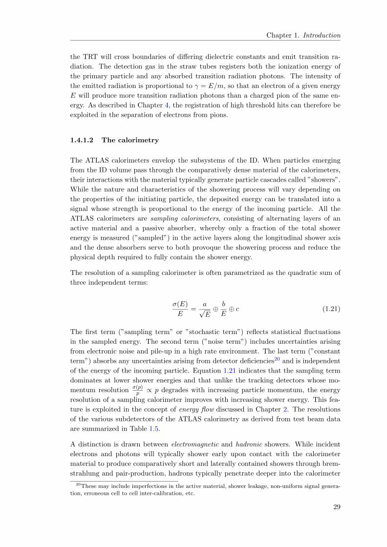
Chapter 1. Introduction
the TRT will cross boundaries of differing dielectric constants and emit transition ra-
diation. The detection gas in the straw tubes registers both the ionization energy of
the primary particle and any absorbed transition radiation photons. The intensity of
the emitted radiation is proportional to γ = E/m, so that an electron of a given energy
E will produce more transition radiation photons than a charged pion of the same en-
ergy. As described in Chapter 4, the registration of high threshold hits can therefore be
exploited in the separation of electrons from pions.
1.4.1.2 The calorimetry
The ATLAS calorimeters envelop the subsystems of the ID. When particles emerging
from the ID volume pass through the comparatively dense material of the calorimeters,
their interactions with the material typically generate particle cascades called ”showers”.
While the nature and characteristics of the showering process will vary depending on
the properties of the initiating particle, the deposited energy can be translated into a
signal whose strength is proportional to the energy of the incoming particle. All the
ATLAS calorimeters are sampling calorimeters, consisting of alternating layers of an
active material and a passive absorber, whereby only a fraction of the total shower
energy is measured (”sampled”) in the active layers along the longitudinal shower axis
and the dense absorbers serve to both provoque the showering process and reduce the
physical depth required to fully contain the shower energy.
The resolution of a sampling calorimeter is often parametrized as the quadratic sum of
three independent terms:
σ(E)
E=
a√E⊕ b
E⊕ c (1.21)
The first term (”sampling term” or ”stochastic term”) reflects statistical fluctuations
in the sampled energy. The second term (”noise term”) includes uncertainties arising
from electronic noise and pile-up in a high rate environment. The last term (”constant
term”) absorbs any uncertainties arising from detector deficiencies20 and is independent
of the energy of the incoming particle. Equation 1.21 indicates that the sampling term
dominates at lower shower energies and that unlike the tracking detectors whose mo-
mentum resolution σ(p)p ∝ p degrades with increasing particle momentum, the energy
resolution of a sampling calorimeter improves with increasing shower energy. This fea-
ture is exploited in the concept of energy flow discussed in Chapter 2. The resolutions
of the various subdetectors of the ATLAS calorimetry as derived from test beam data
are summarized in Table 1.5.
A distinction is drawn between electromagnetic and hadronic showers. While incident
electrons and photons will typically shower early upon contact with the calorimeter
material to produce comparatively short and laterally contained showers through brem-
strahlung and pair-production, hadrons typically penetrate deeper into the calorimeter
20These may include imperfections in the active material, shower leakage, non-uniform signal genera-tion, erroneous cell to cell inter-calibration, etc.
29

Chapter 1. Introduction
Calorimeter subsystem Test beam configuration Resolution σ(E)E (GeV)
ECAL e± (1-250 GeV, |η| = 0.687) 10%√E⊕ 0.17%
ECAL + HCAL barrel π± (10-300 GeV, |η| =0.25) 52%√E⊕ 1.6%
E ⊕ 3%
HCAL end-caps π± (5-200 GeV) 70.6%√E⊕ 5.8%
FCAL e± (10-200 GeV) 28.5%√E⊕ 3.5%
FCAL π± (10-200 GeV) 94.2%√E⊕ 7.5%
Table 1.5: Fractional (single particle) resolutions of the various calorimeter subsys-tems as derived from test beam data [37].
Figure 1.14: Cut-away view of the ATLAS calorimeter, with the various componentsof the electromagnetic, hadronic and forward calorimeters [37].
volume before initiating both broader and longer cascades through strong interactions
with the atomic nuclei21. A good separation between electromagnetic and hadronic
showers is important for particle identification methods, such as those discussed in
Chapter 2, and is usually achieved by employing high-Z absorber materials. High-Z
absorbers also help contain the shower of very high energy particles inside the calorime-
ter volume and minimizes leakage into the muon spectrometer. This hermetic quality of
the calorimeters is vital for an accurate measurement of the missing transverse energy
as is further discussed in Chapter 3 and the desire to capture and contain the full energy
of the interaction also underpins the wide η-coverage provided by the calorimetry.
The components of the ATLAS calorimetry are schematically depicted in Figure 1.14.
The various designs of the electromagnetic, hadronic and forward calorimeters is briefly
21As is explained in Section 2.3.2.2, charged hadronic showers will also contain an electromagneticcore.
30

Chapter 1. Introduction
described below.
The electromagnetic calorimeters
The electromagnetic calorimeter (ECAL) is designed to provide precision measurements
of light electromagnetically interacting particles.
The ECAL employs liquid argon (LAr) as active medium interspersed with steel plated
lead absorbers. The shower particles ionize the LAr and the associated ionization charges
are subsequently collected at electrodes under the influence of an externally applied
electric field.
The need to embed the ID in a magnetic field comes at the cost of insensitive (”dead”)
material in front of the ECAL in the form of a solenoid magnet and a cryostat. In order
to correct for dead material upstream of the calorimeters, a thin layer of presamplers
are installed in front of the ECAL to provide a (partial) recovery of any energy lost in
dead material.
The central section of the ECAL (|η| < 2.5) which overlaps with the η-reach of the ID,
is longitudinally segmented in three layers of differing granularity, as shown in Figure
1.15(a). This design configuration is an essential prerequisite for the particle flow in-
spired studies discussed in Chapter 2. The first layer, the so called η-strip layer, is very
finely segmented in η to provide a means to disentangle showers from closely spaced
photons with origin in π0 → γγ decays from prompt γ showers. While coarser than the
η − strip layer, the middle layer still provides a comparatively fine granularity across
a substantial longitudinal segment of the electromagnetic shower, followed by a thinner
back layer with coarser granularity.
Figure 1.15(a) also indicates that instead of employing a conventional parallel geometry,
the ECAL absorber and readout plates are embedded in a novel accordion geometry,
where the plates follow a zigzag pattern along the direction of the incident particle.
Rather than crossing a series of separate plates, this configuration ensures that the
shower particles cross the same plate repeatedly. With the readout placed on the front
and rear faces of the calorimeter, the accordion geometry secures full and crack-free
azimuthal coverage.
The hadronic calorimeters
The hadronic calorimeter (HCAL) encapsulates the ECAL and is designed to fully con-
tain and measure hadronic showers. The technologies utilized in the barrel and endcaps
differ to better suit the requirements of the local experimental environment.
The two-component tile calorimeter (barrel and extended barrel) makes use of plastic
scintillator tiles interleaved with steel absorber plates. When particles traverse the
active medium, atomic excitations generate scintillation light which is read out by way
of wavelength shifting fibers and photomultipliers.
31
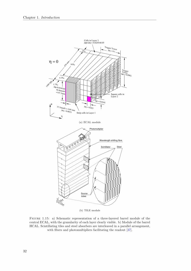
Chapter 1. Introduction
∆ϕ = 0.0245
∆η = 0.02537.5mm/8 = 4.69 mm ∆η = 0.0031
∆ϕ=0.0245x4 36.8mmx4 =147.3mm
Trigger Tower
TriggerTower∆ϕ = 0.0982
∆η = 0.1
16X0
4.3X0
2X0
1500
mm
470 m
m
η
ϕ
η = 0
Strip cells in Layer 1
Square cells in Layer 2
1.7X0
Cells in Layer 3 ∆ϕ×∆η = 0.0245×0.05
(a) ECAL module
Photomultiplier
Wavelength-shifting fibre
Scintillator Steel
Source
tubes
(b) TILE module
Figure 1.15: a) Schematic representation of a three-layered barrel module of thecentral ECAL, with the granularity of each layer clearly visible. b) Module of the barrelHCAL. Scintillating tiles and steel absorbers are interleaved in a parallel arrangement,
with fibers and photomultipliers facilitating the readout [37].
32

Chapter 1. Introduction
(a) Cut-away view of the ATLAS muon spectrometer. (b) Eight-fold arrangement of toroid magnets.
Figure 1.16: The ATLAS muon spectrometer [37].
The more forward regions are exposed to higher radiation doses, rendering plastic scin-
tillator technology unsuitable. Therefore, the hadronic endcaps employ LAr technology
with Cu rod absorbers in a planar geometry configuration.
The forward calorimeters
The forward calorimeters (FCAL) cover the very forward regions 3.1 < |η| < 4.9 and
must therefore operate in an environment where the radiation doses are 30 times higher
than in the endcap region. Consequently, a very different design is required to ensure
containment and fast readout. As indicated in Figure 1.14, the FCAL is segmented in
three layers. The layer closest to the interaction point is optimized for the measure-
ment of electromagnetic showers, while the two subsequent layers function as hadronic
calorimeters. This comparatively fine segmentation allows for the reconstruction of for-
ward jets. Each layer of the FCAL consists of a dense metal matrix interleaved with
active LAr filled tubes running parallel to the beampipe. While Cu is used in the first
layer, tungsten is employed in the outer layers to ensure full containment of the forward
hadronic showers.
As discussed in Chapter 3, an accurate measurement of the missing transverse energy
requires a hermetically sealed detector. The forward calorimeters contribute greatly
towards this end.
1.4.1.3 The Muon Spectrometer
While most particles are fully absorbed in the calorimeters, muons will typically traverse
the entire detector volume as MIPs. This characteristic property enables a clean detec-
tion in the outermost layers of the ATLAS detector, the so called muon spectrometer.
Its distance from the interaction region, makes the muon spectrometer the largest sub-
system in ATLAS. It is embedded in a strong toroidal magnetic field (0.5-1 T) delivered
by a triplet of superconducting air-core toroid magnets (one in the barrel and one in
each endcap) assembled in an eightfold azimuthal arrangement about the beamline, as
33
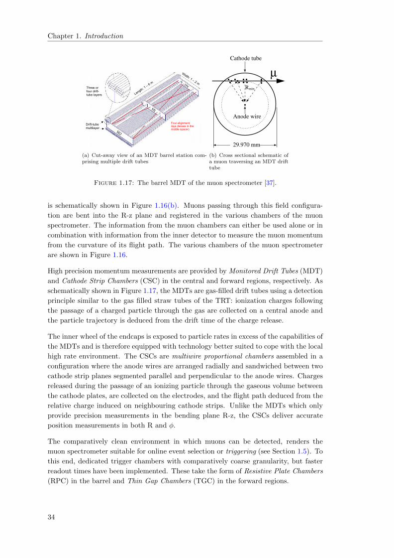
Chapter 1. Introduction
(a) Cut-away view of an MDT barrel station com-prising multiple drift tubes
µ
29.970 mm
Anode wire
Cathode tube
Rmin
(b) Cross sectional schematic ofa muon traversing an MDT drifttube
Figure 1.17: The barrel MDT of the muon spectrometer [37].
is schematically shown in Figure 1.16(b). Muons passing through this field configura-
tion are bent into the R-z plane and registered in the various chambers of the muon
spectrometer. The information from the muon chambers can either be used alone or in
combination with information from the inner detector to measure the muon momentum
from the curvature of its flight path. The various chambers of the muon spectrometer
are shown in Figure 1.16.
High precision momentum measurements are provided by Monitored Drift Tubes (MDT)
and Cathode Strip Chambers (CSC) in the central and forward regions, respectively. As
schematically shown in Figure 1.17, the MDTs are gas-filled drift tubes using a detection
principle similar to the gas filled straw tubes of the TRT: ionization charges following
the passage of a charged particle through the gas are collected on a central anode and
the particle trajectory is deduced from the drift time of the charge release.
The inner wheel of the endcaps is exposed to particle rates in excess of the capabilities of
the MDTs and is therefore equipped with technology better suited to cope with the local
high rate environment. The CSCs are multiwire proportional chambers assembled in a
configuration where the anode wires are arranged radially and sandwiched between two
cathode strip planes segmented parallel and perpendicular to the anode wires. Charges
released during the passage of an ionizing particle through the gaseous volume between
the cathode plates, are collected on the electrodes, and the flight path deduced from the
relative charge induced on neighbouring cathode strips. Unlike the MDTs which only
provide precision measurements in the bending plane R-z, the CSCs deliver accurate
position measurements in both R and φ.
The comparatively clean environment in which muons can be detected, renders the
muon spectrometer suitable for online event selection or triggering (see Section 1.5). To
this end, dedicated trigger chambers with comparatively coarse granularity, but faster
readout times have been implemented. These take the form of Resistive Plate Chambers
(RPC) in the barrel and Thin Gap Chambers (TGC) in the forward regions.
34

Chapter 1. Introduction
The RPC are gaseous parallel plate detectors comprising two opposing electrode plates
sandwiching a gaseous volume. The charges created in the gas following the passage of
a charged particle, drift to the electrodes with a signal width of 5 ns where they are
readout via metallic strips in η and φ. With two gas gaps per RPC station, a total
of six measurements are provided for a charged particle traversing the barrel. These
measurements do not only permit an online selection of muons, but also complements
the precision MDT measurement with an estimation of the φ-coordinate. In the endcaps,
multiwire proportional chamber technology is employed where the bending coordinate
is measured by the anode sense wire and the azimuth by the cathode strips.
The trigger capabilities of the muon spectrometer are exploited in the design of new
triggers in Chapter 4.
1.4.2 The forward detector systems
The central detector is complemented by a set of detector systems extending the total
η-coverage far beyond the reach of the (central) forward calorimeters. These systems
all consist of a pair of identical and equidistant detectors, placed on either side of the
central interaction point.
Rather than enhancing the particle identification capabilities of ATLAS, these detectors
provide a means to identify and trigger on collision events and to monitor and measure
luminosity. The ability to detect collision debris scattered into the extreme forward
directions, make the forward detectors potentially vital tools in tagging various forward
physics processes, such as those discussed in Section 1.3.4.
The location and η-coverage of the various detector systems in ATLAS are depicted in
Figure 1.18(a).
A brief description of the forward detector systems follows below in order of their distance
from the interaction region.
1.4.2.1 MBTS (z= ±3.6 m, 2.12< |η| < 3.85)
Located on the front face of either LAr endcap, the Minimum Bias Trigger Scintillators
(MBTS) actually form part of the central detector, but is herein classified as a forward
detector because of its applicability in forward rapidity gap identification (see Chapter
4). Its primary function is however to act as a trigger for minimum bias processes in
the early phase of LHC operation. As shown in Figure 1.19, each wheel of the MBTS
consists of 16 wedge-shaped plastic scintillators with an eightfold azimuthal segmentation
in two η-rings: an inner ring covering 2.83 < |η| < 3.85 and an outer ring covering
2.12 < |η| < 2.83.
The scintillator light generated by the passage of particles through the scintillating
material is collected by wavelength shifting fibres and amplified by photomultiplier tubes.
If the deposited energy exceeds a threshold value, the signal is communicated to the Level
35

Chapter 1. Introduction
(a) Atlas pseudorapidity coverage
(b) η-spectrum of >100 MeV particles from simulated non-diffractive minimum bias events(PYTHIA) with the fractional coverage provided by the central detector (CD), MBTS, FCAL,LUCID, ZDC and ALFA.
Figure 1.18: The location and η-coverage various ATLAS detector subsystems.
36

Chapter 1. Introduction
Figure 1.19: MBTS disk configuration. One such disk is placed on the inside of eachLAr endcap. [40].
1 trigger (see Section 1.5) which is able to execute a logical AND/OR on signals from either
side of the interaction point. This feature is exploited in Chapter 4 for triggering on
lepton final states from exclusive production processes. The lifetime of the MBTS is
limited to the early phase of LHC running at comparatively low luminosity, after which
the plastic scintillators will deteriorate from excessive radiation exposure [35].
1.4.2.2 LUCID (z=±17 m, 5.4< |η| <6.1)
Located at a distance of 17 m from the interaction point, LUCID (LUminosity mea-
surement using Cerenkov Integrating Detector) is principally designed to monitor the
instantaneous luminosity and beam conditions through the detection of forward scat-
tered debris from inelastic pp collisions. As the number of charged particles detected
is proportional to the number of interactions in a bunch crossing, a rapid luminosity
determination is made possible by evaluating the average number of interactions per
bunch crossing.
When charged particles traverse one of the several Cerenkov tubes arranged parallel
to the beamline, they emit Cerenkov light22 which can be collected by photomultipli-
ers. The magnitude of the collected signal will be indicative of the number of particles
crossing the tube, while ultrafast timing (∼100 ps) allows for a precise separation of
subsequent bunch crossings.
As discussed in Chapter 4, LUCID could also be used to identify forward rapidity gaps
and tag exclusive processes.
22Cerenkov light is electromagnetic radiation emitted when a charged particle passes through a mediumat a constant speed greater than the speed of light in that medium.
37

Chapter 1. Introduction
1.4.2.3 ZDC (z=±140 m, |η| >8.3)
At a distance of 140 m from the interaction point, the ZDC (Zero Degree Calorimeters)
are located where the single ”interaction” beampipe bifurcates into two separate beam-
lines. While charged particles are largely deflected by the beam magnets, the ZDC will
readily absorb forward neutral debris from the interaction, such as γ, π0 and neutrons.
The ZDC consists of one electromagnetic and three hadronic sampling calorimeters,
each module containing several layers of active quartz rods interleaved with tungsten
absorbers.
The ZDC are integral to the detection of forward neutrons from ultraperipheral heavy
ion collisions (see Section 4.7), but also find applications as additional minimum bias
triggers, as a beam gas and beam halo background suppressor23 and in early beam
tuning.
1.4.2.4 ALFA (z=±240 m, 10.6< |η| <13.5)
While LUCID provides relative luminosity monitoring, ALFA (Absolute Luminosity For
Atlas) aims to provide ATLAS with an accurate measurement of the absolute luminosity
delivered24. This is achieved through the detection of elastic pp collisions down to very
small scattering angles25.
To facilitate the measurement of small angle deflections, ALFA is located far from the
interaction point and employs Roman Pot technology wherein scintillating fiber trackers
are moved to a distance of only ∼ 1 mm from the beam from above and below. This
is only possible in dedicated runs when the beam configuration and optics is especially
tuned to ensure the beam divergence does not exceed the small elastic scattering angles.
ALFA may also be used to tag fully elastic exclusive scatters, such as depicted in Figure
1.7(b), by detecting the photon emitting proton whose flight path after emittance is only
slightly deflected with respect to the overall beam direction.
1.4.2.5 AFP - ATLAS Forward Proton Project
In addition to the forward detector systems presented above, ATLAS is currently in-
volved in a joint pan-experimental26 R&D project to evaluate the feasibility of installing
proton tagging detectors at 420 m from the nominal IP to either side of both ATLAS
and CMS [29].
23A tight coincidence requirement on either ZDC can help reduce backgrounds from beam effects.24The relative luminosity is typically derived from fast, reproducible measurements and is propor-
tional to the actual luminosity in an unknown, but constant way. By contrast, an absolute luminositymeasurement is typically derived from beam parameters or a well known physics process.
25The optical theorem relates the forward elastic scattering amplitude to the total cross section σtot,the latter from which the absolute luminosity can be determined.
26The FP420 project involves members from the ATLAS, CMS and TOTEM experiments, as well asaccelerator scientists and theorists.
38

Chapter 1. Introduction
The proposed detector systems are designed to operate as a magnetic spectrometer.
Protons losing a minute fraction of their longitudinal momenta in a bunch crossing in-
teraction, will typically continue undetected down the beampipe. As the bunch travels
along the beamline, the LHC dipole magnets will bend protons carrying a small trans-
verse component into the extremities of the beam envelope. At 420 m from the nominal
interaction point, these protons ”decouple” from the beam and are detected in several
consecutive near-beam silicon tracker planes.
Spatial restriction precludes the use of Roman Pot techniques [41], therefore the proposal
foresees the use of a ”moving beampipe” in which segments of the LHC beampipe are
replaced by custom beampipe modules with a larger diameter and a flattened area
along one side where the tracking and timing detectors are located. Bellows connect
the modules to the LHC beampipe to allow the sensors to be retracted during beam
injection and moved closer to the beam during collisions. In this fashion, FP420 aims
to tag and measure protons with fractional momentum losses of order 0.2-2%.
The proton arrival time is measured by the fast Cerenkov timing detectors. This timing
information provides a measure for the time of flight from the interaction point and
consequently the z-position of the interaction vertex. This in turn, may permit the
tagging of e.g. elastic two-photon processes in a high luminosity environment with large
pile-up contributions.
A major benefit to be derived from the FP420 project is the ability to precisely measure
the proton momentum losses ξ. The mass of the centrally produced system can then be
measured to high resolution (∼ 2-3 GeV) on an event-by-event basis using the missing
mass method [29]:
M ∼√ξ1ξ2s (1.22)
where√s is the center of mass energy of the colliding protons. Since this method relies
squarely on forward proton tagging, it can be applied to determine the mass of any
(resonant) exclusive central system, regardless of how the central system decays.
1.5 Trigger and Data Acquisition
At design luminosity, the LHC will cross bunches 40 million times per second. With an
average event size of ∼ 1.3 MB, it is technically unfeasible to record collision events at
a rate in excess of ∼ 200 Hz. The ATLAS trigger and data acquisition (DAQ) decides
which 5 per million collision events will be recorded for later offline analysis.
As shown in Figure 1.20, ATLAS employs a three-tiered trigger scheme providing an
overall rate reduction from 40 MHz to 200 Hz.
The Level 1 (L1) trigger is required to make a decision every 25 ns and therefore needs
to operate with very short processing times. Custom designed hardware allows time-
stamped information from the various detector systems corresponding to roughly 100
39

Chapter 1. Introduction
Figure 1.20: Schematic representation of the three tiered ATLAS trigger system.
successive bunch crossing to be stored in a memory buffer. With a latency of 2 µs,
information from multiple bunch crossings is processed simultaneously by the Central
Trigger Processor, which decides whether the event should be discarded or passed on to
the Level 2 trigger for further processing. The decision is based on a predefined catalogue
of thresholds associated with crude signatures compatible with a µ, e/γ, hadronically de-
caying τ , jet or EmissT , as well as some combinations thereof. While muon signatures
are extracted from the muon trigger chambers, all other signatures derive from course
granular (η × φ ∼ 0.1 × 0.1) information drawn from the calorimeters alone. No in-
formation from the inner detector is available at L1. If a positive decision is passed, a
Region of Interest (RoI) in η−φ is built about the triggered objects and the full detector
granularity within these RoIs passed to L2. This seeded approach significantly reduces
the amount of data transfered and facilitates a speedy trigger decision.
Unlike the L1 trigger, the two subsequent trigger levels27 are processing farms built from
commercially available computer technology. The Level 2 (L2) algorithms are seeded
by the RoIs provided by L1 and have access to the full detector granularity therein,
including information from the inner detector. Dedicated software is used to reconstruct
and identify signatures within an RoI, enabling a refined decision with respect to L1 and
a rate reduction from 75 kHz to 3.5 kHz within a latency of ∼40 ms per event.
The Event Filter (EF) by contrast, is not limited to the information within the RoI, but
has full access to the complete detector granularity. This makes the EF comparatively
slow (∼ 4 s/event), but enables a much more refined decision based largely on the output
of the offline reconstruction algorithms. The raw data of events passing the EF is written
out to a central storage at a rate of ∼ 200 Hz, with a copy immediately distributed to
27The two upper levels of the ATLAS trigger are collectively termed the Higher Level Trigger (HLT)
40
Chapter 1. Introduction
one of ten Tier 1 grid computing nodes worldwide wherein it is processed and made
available for detailed offline analysis to all members of the collaboration.
The ATLAS trigger configuration is steered by a trigger menu approved by the collab-
oration. The trigger menu provides a catalogue of trigger chains of which at least one
must pass for the event to be recorded to storage. A trigger chain stipulates a sequence
of criteria or signatures that must be met at each level of the trigger for the chain to
pass. To ensure that the total accept rate at the EF does not exceed the upper limit of
200 Hz, some signatures are assigned prescale factors. A prescale factor of 1000 implies
that only 0.1% of events satisfying the signature requirements are eligible to pass. The
combined prescale on a chain is therefore the product of the prescales applied to the
signatures at each level. Both chain configurations and the application of prescale fac-
tors will evolve with the instantaneous luminosity delivered by the LHC. The choice of
trigger menu and the configuration of the chains therein may therefore severely impact
the feasibility of offline analyses. These issues are further discussed in Chapter 4.
1.6 A note on Monte Carlo simulations
The complexity associated with an experiment like ATLAS render simulation tools in-
dispensable in nearly all areas of both ATLAS operation and data analysis. Simulated
data are not only required to compare recorded data with theoretical predictions, but
equally so for testing and evaluating the impact of instrumental effects on recorded data
and for the development and validation of both new and existing offline reconstruction
algorithms. Simulation tools thus provide robust modeling of the expected instrumental
response to a given physical phenomena in a particular experimental environment to
high statistical accuracy. In this context, it is appropriate to distinguish between the
simulation of a physical interaction process and the simulation of the passage of stable
particles emerging from the interaction region through the experimental volume.
The simulation of a physical interaction process encompasses all stages of a scattering
interaction, including the hard interaction, hadronization and decay, as well as the under-
lying event. The modeling of these processes is generic, insofar that it does not depend
on the details of the experimental volume in which the processes occur and are typically
handled either by one single or a combination of several Monte Carlo Generators [20].
The stable particle output of such Monte Carlo Generators is then fed into an experiment-
specific detector simulation which provides a stepwise propagation of each final state par-
ticle through a virtual detector volume, (ideally) taking due account of all interactions
with matter along the trajectories. In ATLAS, this virtual detector volume is provided
by a GEANT4 simulation tool [42] configured with an accurate mapping of the material
distribution inside of ATLAS.
The simulated interactions with the detector material are then translated (”digitized”)
into a format identical to that in which real data is recorded.
41
Chapter 1. Introduction
The subsequent steps involve the translation (”reconstruction”) of raw (simulated or
recorded) data into lower level objects such as tracks and clusters and subsequently
higher level objects such as electrons and taus, whereby information is typically combined
from several different detector systems.
Limited only by the accuracy of the detector modeling and the description of particle
interactions with the detector material, a full GEANT-based simulation will mostly
deliver statistically accurate results at the cost of comparatively prolonged computing
times. Depending on the particle multiplicity of the physical process under examination,
the average CPU-time required for the simulation of a single event will be of O ∼ 20
min.
Long simulation times severely limit the viability of producing large samples of full
GEANT-based simulated data. As is discussed in Chapter 3, the consequences of insuf-
ficient amounts of simulated data can be detrimental for physics analyses. More recent
developments therefore attempt to partially alleviate this problem by trading moder-
ate reductions in simulation accuracy for significant reductions in simulation times.
This is typically achieved by either simplifying the configured detector geometry or by
parametrizing the energy response of particles in the detector (or a combination of both)
[43, 44].
42

Chapter 2
Tau Reconstruction and
Identification
2.1 Introduction
The tau lepton (τ) and the tau neutrino (ντ ) together make up the third generation of
leptons in the SM1. In the chiefly hadronic environment of the LHC, leptons often count
among the most important handles on the hard interaction of interest. As the heaviest
lepton in the SM, the τ -lepton plays an integral part in the ATLAS physics programme,
not only in the context of the SM, but notably also in many searches for potentially new
physics beyond.
The central role played by the τ -lepton across such broad range of interesting physics
processes, underpins the need for efficient offline reconstruction and identification mech-
anisms with the ability to furnish offline analyses with the maximal amount of relevant
information. This chapter will concern itself with the reconstruction and identification
of τ -leptons. After a review of the key properties of tau leptons and the their place
within the LHC physics programme, the canonical approaches to τ -reconstruction are
briefly summarized before a novel method of reconstructing and identifying tau leptons
is introduced.
2.1.1 The decay phenomenology of the τ-lepton
With a mass of 1,776.84 ± 0.17 MeV [38], the τ -lepton is unique in that it is the
only lepton to exhibit decays into hadrons as well as into its lighter counterparts the
electron and muon. As shown in Figure 2.1, all τ -lepton decays pass by way of the weak
interaction through the exchange of a virtual W boson. Lepton number conservation
implies that all τ -lepton decays involve a ντ which necessarily renders a portion of the
τ four-vector experimentally undetectable. The W couples with universal strength to
1Incidentally, the tau lepton was the first member of the third generation of fermions to be discovered[45], an achievement for which M. Pearl was awarded the 1995 Nobel Prize in physics.
43
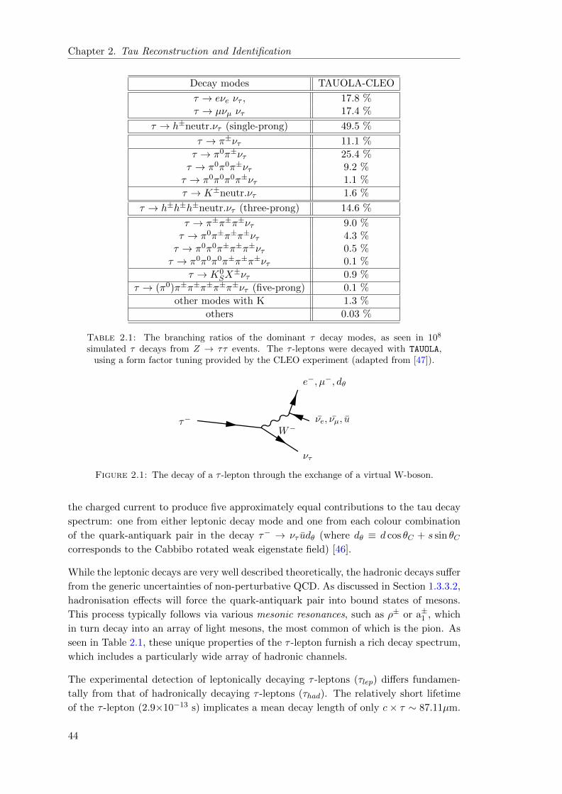
Chapter 2. Tau Reconstruction and Identification
Decay modes TAUOLA-CLEO
τ → eνe ντ , 17.8 %τ → µνµ ντ 17.4 %
τ → h±neutr.ντ (single-prong) 49.5 %
τ → π±ντ 11.1 %
τ → π0π±ντ 25.4 %τ → π0π0π±ντ 9.2 %τ → π0π0π0π±ντ 1.1 %
τ → K±neutr.ντ 1.6 %
τ → h±h±h±neutr.ντ (three-prong) 14.6 %
τ → π±π±π±ντ 9.0 %τ → π0π±π±π±ντ 4.3 %τ → π0π0π±π±π±ντ 0.5 %τ → π0π0π0π±π±π±ντ 0.1 %
τ → K0SX±ντ 0.9 %
τ → (π0)π±π±π±π±π±ντ (five-prong) 0.1 %
other modes with K 1.3 %
others 0.03 %
Table 2.1: The branching ratios of the dominant τ decay modes, as seen in 108
simulated τ decays from Z → ττ events. The τ -leptons were decayed with TAUOLA,using a form factor tuning provided by the CLEO experiment (adapted from [47]).
W−τ−
ντ
νe, νµ, u
e−, µ−, dθ
Figure 2.1: The decay of a τ -lepton through the exchange of a virtual W-boson.
the charged current to produce five approximately equal contributions to the tau decay
spectrum: one from either leptonic decay mode and one from each colour combination
of the quark-antiquark pair in the decay τ− → ντ udθ (where dθ ≡ d cos θC + s sin θCcorresponds to the Cabbibo rotated weak eigenstate field) [46].
While the leptonic decays are very well described theoretically, the hadronic decays suffer
from the generic uncertainties of non-perturbative QCD. As discussed in Section 1.3.3.2,
hadronisation effects will force the quark-antiquark pair into bound states of mesons.
This process typically follows via various mesonic resonances, such as ρ± or a±1 , which
in turn decay into an array of light mesons, the most common of which is the pion. As
seen in Table 2.1, these unique properties of the τ -lepton furnish a rich decay spectrum,
which includes a particularly wide array of hadronic channels.
The experimental detection of leptonically decaying τ -leptons (τlep) differs fundamen-
tally from that of hadronically decaying τ -leptons (τhad). The relatively short lifetime
of the τ -lepton (2.9×10⁻¹³ s) implicates a mean decay length of only c× τ ∼ 87.11µm.
44

Chapter 2. Tau Reconstruction and Identification
If the decay proceeds leptonically, there is little to distinguish the visible decay products
from primary electrons or muons, save by way the non-zero impact parameter exhib-
ited in their tracks. The challenges associated with this task have traditionally been
considered too involved to actively pursue in an LHC environment, though recent work
has uncovered considerable scope in the channel τ → ντνµµ [48]. The presence of an
additional neutrino further implies that the visible energy available in a leptonic de-
cay will be less than that available in a hadronic decay for a tau of a given energy, a
feature which at low transverse momenta may further challenge the reconstruction and
identification of τlep.
The focus in ATLAS, as indeed herein, is therefore placed on the identification of hadron-
ically decaying τ -leptons, which account for roughly 65% of all τ -lepton decay modes. As
is seen in Table 2.1, such decays are characterized by an odd number of charged mesons,
of which ∼ 95% involve either one or three pions. In the parlance of τ -physics, a hadronic
decay into n charged particles is commonly termed an n-prong mode in reflection of the
number of charged tracks associated with the decay.
As indicated in Table 2.1, 1-prong modes account for roughly 76% of all τhad, whereas
the rest is dominated by various 3-prong modes. The comparatively scarce occurrence
of n > 3 modes, precludes their consideration in the context of ATLAS and herein.
Table 2.1 further indicates that each n-prong decay may include a neutral component,
most commonly in the form of neutral pions. This is particularly true of 1-prong modes,
where almost 74% of all decays involve at least one π0. Among the 3-prong modes,
additional π0 are more rare, occurring in roughly 1/3 of all 3-prong decays.
While the majority of hadronic decays involve π± and π0, a small fraction of decays will
involve strange mesons, such as K±s and K0s s. From the experimental point of view,
decays into π± and K± are mostly equivalent. The K0s primarily decays into either two
charged pions or two neutral pions. Depending on just how they interact within the
detector, decays involving K0s s may hence be registered as either 1-prong or 3-prong.
In summary, a hadronically decaying tau is therefore principally identifiable by way of
its unique decay topology:
• 1 or 3 tracks from the π±s,
• hadronic energy depositions from the π±s,
• potential electromagnetic energy depositions from the π0 → γγ.
2.1.2 The role of tau leptons in the LHC physics programme
The comparatively complex decay phenomenology of the τ -lepton arguably makes it
the most challenging charged lepton to reconstruct and identify in the predominantly
hadronic environment of the LHC. As was already alluded to in Chapter 1, the abundance
of hadronic debris from various QCD processes constitutes a formidable background to
45
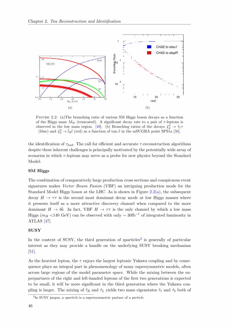
Chapter 2. Tau Reconstruction and Identification
(a) (b)
Figure 2.2: (a)The branching ratio of various SM Higgs boson decays as a functionof the Higgs mass MH (truncated). A significant decay rate to a pair of τ -leptons isobserved in the low mass region. [49]. (b) Branching ratios of the decays χ0
2 → τ1τ(blue) and χ0
2 → lRl (red) as a function of tanβ in the mSUGRA point SPS1a [50].
the identification of τhad. The call for efficient and accurate τ -reconstruction algorithms
despite these inherent challenges is principally motivated by the potentially wide array of
scenarios in which τ -leptons may serve as a probe for new physics beyond the Standard
Model:
SM Higgs
The combination of comparatively large production cross sections and conspicuous event
signatures makes Vector Boson Fusion (VBF) an intriguing production mode for the
Standard Model Higgs boson at the LHC. As is shown in Figure 2.2(a), the subsequent
decay H → ττ is the second most dominant decay mode at low Higgs masses where
it presents itself as a more attractive discovery channel when compared to the more
dominant H → bb. In fact, VBF H → ττ is the only channel by which a low mass
Higgs (mH <140 GeV) can be observed with only ∼ 30fb−1 of integrated luminosity in
ATLAS [47].
SUSY
In the context of SUSY, the third generation of sparticles2 is generally of particular
interest as they may provide a handle on the underlying SUSY breaking mechanism
[51].
As the heaviest lepton, the τ enjoys the largest leptonic Yukawa coupling and by conse-
quence plays an integral part in phenomenology of many supersymmetric models, often
across large regions of the model parameter space. While the mixing between the su-
perpartners of the right and left-handed leptons of the first two generations is expected
to be small, it will be more significant in the third generation where the Yukawa cou-
pling is larger. The mixing of τR and τL yields two mass eigenstates τ1 and τ2 both of
2In SUSY jargon, a sparticle is a supersymmetric partner of a particle.
46
Chapter 2. Tau Reconstruction and Identification
which frequently appear in SUSY phenomenology to which ATLAS may be sensitive.
An illustrative case in point is found in mSUGRA-type models, wherein the τ1 is the
lightest slepton and moreover receives a significant τL-contribution thereby enhancing
its coupling to the wino-dominated light gauginos χ02 and χ±1
3. An inherent tendency
for τ -lepton final states therefore exists, a characteristic often made more pronounced
in scenarios with large tanβ, as shown in Figure 2.2(b).
τ -leptons may then readily appear in the decay of strongly produced squarks and gluinos:
q → qχ02 → qτ±τ∓ → qτ±τ∓χ0
1
and their successful reconstruction hence provide a handle on the masses and mixings
of SUSY particles in the decay chain [52]. Moreover, the polarization of the τ -leptons
in the above decay chain will depend on the precise bino/wino/higgsino content of the
χ01 and χ0
2 and thus deliver valuable information on their respective couplings, as well
as that of τ± [53]. An accurate polarization dependent measurement requires the τ -
reconstruction algorithms to not only be able to suppress unwanted background, but
also to facilitate the evaluation of the precise decay mode of the τ -lepton [53]. The need
for an efficient separation of the various decay modes of the τ -lepton, partially motivates
the development of the novel τ -reconstruction algorithm presented herein.
MSSM Higgs
A minimal supersymmetric extension to the Standard Model comes with two Higgs
doublets, giving rise to altogether three neutral (h, H, A) and two charged (H±) physical
states.
The decay of the charged Higgs is expected to be dominated by H± → tb and H± →τντ , the latter of which provides a more promising avenue for observation in the QCD
environment of the LHC. If observed, a rate measurement of H± → τντ may help
determine the value of the SUSY parameter tanβ [54]. The neutral Higgs states H and
A are also predicted to decay into a pair of τ -leptons, with rates significantly larger
than the corresponding rate of the Standard Model Higgs across a large portion of the
parameter space.
Standard Model
The decay process W → τντ is the most copious Standard Model source of (isolated)
τ -leptons at the LHC and consequently plays an integral role in the early commission-
ing and consolidation of τ -reconstruction and identification tools. However, the most
important process for early commissioning is arguably the process Z → ττ . Despite
a cross section roughly an order of magnitude below that of W → τντ , the presence
of an additional τ -lepton in the event not only serves to suppress backgrounds, but
also allows for an unbiased collection of τhad through the explicit selection of events
in which one τ -lepton decays leptonically and the other hadronically. This invites for
3The wino only couples to lL. A large wino-admixture therefore suppresses the coupling to othersleptons.
47

Chapter 2. Tau Reconstruction and Identification
Figure 2.3: Visible transverse energy spectrum of τ -leptons in various processes atthe LHC, normalized to their respective predicted cross sections (
√s = 14 TeV) and
an integrated luminosity corresponding to 10 fb−1 [32].
the use of tag-and-probe techniques to measure online and offline reconstruction efficien-
cies. In addition, a peak is expected to manifest itself in the visible mass spectrum, a
feature which in turn can be exploited in the determination of the τhad energy scale.
Another prolific source of τ -leptons may be found in semi-leptonic tt events, where
tt→ W (→ qq)W (→ τhadντ )bb or tt→ W (→ eνe/µνµ)W (→ τhadντ )bb. While the cross-
sections are smaller than for Z/W, so are backgrounds, and the unique event topology
of tt events allows one to test τ -lepton identification in an environment much resembling
that predicted of SUSY. The Standard Model also predicts τ -final states resulting from
two-photon processes at the LHC. While the observation of such events remains elusive
at hadron colliders, the potential for their detection is discussed at length in Chapter 4.
2.1.3 Kinematics of tau decays at the LHC and challenges to tau re-
construction
The wide array of physics processes in which τ -leptons are anticipated to play a central
role calls for efficient reconstruction algorithms across a broad kinematic range, as is
indicated in Figure 2.3.
While the high end of the kinematic spectrum is relevant for searches involving heavy
new particles decaying into a pair of τ -leptons, it is noteworthy that the lower end is
relevant to not only Standard Model processes, but also to VBF Higgs and SUSY. The
latter is a peculiar case in point, whereby a small mass difference m(τ1)-m(χ01). 30 GeV
will typically imply that τ -leptons emerging from the decay τ1 → τ χ01 will tend to be
comparatively soft.
In the hadronic environment of the LHC, the central challenge to the τ -reconstruction
will nearly always be to suppress the overwhelming background from QCD processes
whose cross section is typically many orders of magnitude larger than the process of
interest. However, subtle, yet important, differences do exist across the various kinematic
regions.
48

Chapter 2. Tau Reconstruction and Identification
(a)
|η|0 0.5 1 1.5 2 2.5
Effic
ienc
y
0.7
0.75
0.8
0.85
0.9
0.95
1
= 100 GeVTp = 5 GeVTp = 1 GeVTp
(b)
Figure 2.4: (a) Maximal distance in ∆R between constituent particles in τ -decaysfrom Z → ττ vs the true visible transverse momentum of the parent τ -lepton. While themajority of will rarely have a spread greater than ∆R ∼ 0.2, low (b) Track reconstruc-tion efficiency for pions at various transverse energies as a function of |η|. Efficiencydegradation is likely to follow from hadronic interactions (and multiple scattering) in
the inner detector material [32].
As was alluded to in Section 2.1.1, the conventional strategy for separating τ -leptons
from QCD jets relies on the characteristic tendency of the former to produce compara-
tively narrow and well collimated ”τ -jets” formed by a limited number of charged and
neutral pions. Quarks and gluons by contrast, will often be colour connected to other
particles in the event and are generally expected to produce broader, less collimated jets
with higher particle multiplicities.
While this property holds very well at intermediate transverse momenta (& 30 GeV), it
is less robust in the high and low ends of the kinematic spectrum. At high transverse
momenta, the Lorentz boost given to the constituents of hadronic jets is likely to make
the resulting jet appear more collimated and consequently more τ -like. As the momenta
of the charged pion constituents of the τ -decay drop, their bending in the magnetic
field of the inner detector becomes more pronounced, effectively widening the τ -jet by
increasing the distance between its pion constituents. This tendency is observed in
Figure 2.4(a) in which the maximum distance of pion constituents from the visible τ -
axis is shown as a function of the visible transverse momentum. The steeply falling QCD
jet cross section at the LHC, also implies that the low-pT region will need to withstand
significantly higher background rates.
Even in cases where the ”narrow-jet” approximation holds well, it is from the perspec-
tive of physics analyses often desirable to not only reconstruct the τ -lepton, but also to
extract potentially valuable information from its mode of decay. This requires the recon-
struction algorithms to not simply view the τ -decay as a unit entity, but also whenever
possible resolve the constituent decay particles. The ability to do so will in large part
depend on both the kinematics and topology of the τ -decay and the interaction of the
decay particles with the detector material:
The relatively large amount of material in the ATLAS inner detector may occasionally
cause charged pions to initiate showering before reaching the calorimeters. As seen in
49
Chapter 2. Tau Reconstruction and Identification
Figure 2.4(b), this effect is slightly more pronounced at low pion energies and such early
hadronic interactions will serve to complicate the identification of τ -decay constituents.
In a similar vein, the relatively short lifetime of the π0 (8.4×10⁻¹⁷s) implies a subsequent
instantaneous decay on detector length scales. In > 98% of cases, the π0 will decay into
two photons (π0 → γγ). The photons from the π0 decay are in turn prone to convert
into electron-positron pairs (γ → e+e−) upon interaction with the material in the inner
detector, before reaching the calorimeters. Additional tracks from photon conversions
may distort the proper reconstruction of the tau decay, e.g. by causing 1-prong decays
to be falsely reconstructed as 3-prong or if the parent π0 is of low momentum result in
a scatter of the neutral energy both within and outside the τ -decay cone4.
In the following, a brief overview of existing approaches to the experimental detection
of tau leptons in ATLAS is presented, before a novel method of reconstructing and
identifying tau leptons is introduced.
2.2 Conventional approaches to tau reconstruction and iden-
tification in ATLAS
The ATLAS experiment currently employs two complementary approaches for the re-
construction and identification of hadronically decaying τ -leptons. By and large, both
algorithms treat the τ -decay as a unit entity and separation from QCD jets is attempted
on the basis of the conspicuous traces left in the tracker and calorimeters:
• a low track multiplicity in a narrow cone
• calorimetric shower shapes and characteristics of the track system
• isolation from other objects in the inner detector and calorimeters
The two algorithms are commonly distinguished in terms of their respective methods for
building a τ -candidate: the calorimeter-based algorithm (tauRec) creates τ -candidates
from jets built on calorimeter clusters, whereas the track-based algorithm (tau1p3p)
builds τ -candidates around good quality tracks. Either algorithm combines information
from both the calorimeters and tracker to construct a suite of discriminating variables on
which either cut-based selections or more complicated multivariate separation methods
can be applied. The implementation is such that both algorithms run in a merged
configuration, so that if a τ -candidate is seeded by both algorithms, variables from
either algorithm are made available for an improved identification.
In the following, only a cursory overview of either method will be given. More detailed
descriptions are available in [47, 55, 56].
4Soft conversion electrons are more sensitive to the magnetic field of the inner detector and mayconsequently be bent out of the τ -decay cone, potentially rendering a portion of the visible τ -momentumlost to the reconstruction.
50

Chapter 2. Tau Reconstruction and Identification
Calorimeter based reconstruction
The calorimeter based candidates are seeded by fixed size cone (∆R =0.4) jets built
on topological calorimeter clusters5. The topological clustering algorithm is described
Section 2.3.1.1. The seed jets are required to satisfy pjetT > 10 GeV and |ηjet| < 2.5. Any
qualified tracks found within a cone of ∆R < 0.3 are associated to the τ -candidate.
Track based reconstruction
Rather than using jets built from calorimeter clusters, the track based τ -candidates are
seeded by qualified tracks with ptrkT > 6 GeV. The core region around the seed track
(∆R < 0.2) is subsequently scanned for additional tracks, and if satisfactory tracks are
found (ptrkT >1 GeV) these are associated to the τ -candidate. If the total number of
tracks exceeds eight, the track-based candidate is discarded. Moreover, the total charge
on a 3-track candidate must satisfy |Q| = 1.
If a calorimeter seeded candidate and a track seeded candidates are found to overlap in
a cone of ∆R < 0.2, only one τ -candidate is built. A reconstructed event may therefore
contain a mixture of τ -candidates that have either been seeded by both the calorimeter
and track based approaches, or alternatively by either one of the two.
2.2.1 Tau energy determination
Two distinct methods for determining the τ energy scale are provided. In calorimeter-
seeded candidates, all calorimeter cells within a cone ∆R < 0.4 about the barycenter
of the seed jet are summed and weighted with an H1-style calibration scheme [58] in
which the cell weights are η, φ and subdetector dependent functions of the cell. This
method was originally intended for jet calibration and consequently (Monte Carlo de-
rived) correction factors are applied to the cell weights to make them more applicable
to τ -jets.
The track based tau candidates by contrast employ an energy flow algorithm to deter-
mine the energy scale of the tau. To do so, the cells associated with the track seeded
candidate are classified in different categories:
• pure electromagnetic energy (EemclT ), involving energy collected in a narrow
window about an isolated electromagnetic cluster displaying minimal hadronic
leakage
• charged electromagnetic energy (EchrgEMT , EchrgHAD
T ), involving energy in
a narrow window about the impact point of the tracks in the each layer of the
calorimeter
• neutral electromagnetic energy, (EneutEMT ), involving energy from all unused
cells surrounding the cell (∆R=0.2) closest to the track impact point in the first
three layers of the calorimeter.
5At the time of writing, the fixed size cone 0.4 jet input is being replaced by Anti-Kt 0.4 jets [57].The latter are also made to run on topological clusters.
51

Chapter 2. Tau Reconstruction and Identification
Assuming the absence of hadronic neutrals, the total charged energy deposition EchrgEMT
+ EchrgHADT are duly replaced by the momenta of the tracks. The potential presence of
π0 mesons is contained in the EemclT and EneutEM
T . Two additional empirically derived
correction terms arise from the potential overlap between π+ and π0 where both deposit
energy in the same cells (∑
resEchrgEMT ) and from charged hadronic leakage outside a
narrow cone about the track(s) (resEneutEMT ). The energy scale of the tau is finally
defined as:
EeflowT =
∑ptrack systemT + Eemcl
T + EneutEMT +
∑resEchrgEM
T + resEneutEMT (2.1)
The motivational backdrop for replacing the energy deposits of cells matched to tracks
in this fashion to obtain an improved energy measurement, is discussed in the following
section.
2.2.2 Tau identification
Both algorithms provide a handful of discriminating variables to assist the suppression
of false candidates from QCD jets. These variables are built from the candidate tracks
or associated calorimeter cells, and include among others:
• The profile (radius) of energy deposits in the electromagnetic calorimeters
• Isolation quantities drawn from calorimeter deposits and tracks in an isolation
region
• Ratio of calorimetric energy to the sum of track transverse momenta
• Track widths6, impact parameter significance of leading track and the transverse
flight path significance of the τ -candidate vertex
A detailed listing of all available variables can be found in [55]. These variables form the
input to various identification methods, ranging from comparatively simple cut-based
approaches to more advanced methods making use of different multivariate techniques.
2.3 The case for energy flow in ATLAS
The principles of energy flow were first applied to jets at LEP by the ALEPH collabo-
ration [59], and the merits of the this approach were later corroborated at other collider
experiments, such as HI, D0 [60] and CDF [61].
Studies of jet fragmentation performed at LEP have revealed the particle composition of
a jet to be roughly 62% charged hadrons, 27% photons, 10% long lived neutral hadrons
6The variance of track ∆η weighted by the track pT , where ∆η is measured with respect to theτ -candidate axis.
52

Chapter 2. Tau Reconstruction and Identification
= 0! (GeV) at T P0 50 100 150 200 250 300 350 400
Reso
lutio
n
0
0.02
0.04
0.06
0.08
0.1
0.12
Calorimeter
Tracking
Figure 2.5: The relative energy resolution (σ(E)/E) and momentum resolution(σ(pT )/pT ) as a function of the π± transverse momentum in ATLAS [62].
(e.g. n, KL) and a small fraction (∼ 1%) of neutrinos [60]. It follows that > 70%
of the jet energy will be measured in the hadronic calorimeters and by consequence
the jet energy resolution will be limited by the comparatively poor resolution of the
hadronic calorimeters. As is shown in Figure 2.5, an improved resolution can be achieved
at low and intermediate transverse momenta, if the calorimetric energy deposits from
charged particles are removed and replaced by their more accurately measured track
momenta. With the momenta of charged particles measured in the tracking detectors,
the calorimeters are only used to determine the energies of photons and neutral hadrons
and consequently the dependence on the hadronic calorimeters is reduced to a minimum.
The challenge will be to properly associate tracks and calorimeter deposits and to avoid
any double counting of energy.
With the advent of more granular calorimeters increasingly more capable of separating
showers from close lying particles, the concept of energy flow has been extended to in-
clude the full reconstruction of the 4-vectors of individual particles in the event, drawing
on the most favourable combination of information from all subdetectors [60, 63]. In this
concept, often known as particle flow, composite particle objects such as τ -leptons and
jets are not treated as unit entities, but instead as objects derived from the reconstructed
particles (π±, π0, γ, µ±,p, n, etc.) in the event.
In the following, it is shown how the ATLAS calorimeters may lend themselves to energy
flow calorimetry, followed by a brief description of the generic energy flow algorithm in
ATLAS. Finally, in Section 2.4, a novel approach to τ reconstruction inspired by the
ideas of particle flow is presented.
53

Chapter 2. Tau Reconstruction and Identification
2.3.1 Clustering of calorimeter cells in ATLAS
The ATLAS calorimeters are described in Section 1.4.1.2. As explained therein, most
particles traversing the calorimeter material are prone to ”shower”, depositing their en-
ergy in several different calorimeter cells across the various layers of the calorimeter, both
along (longitudinally) and perpendicular (laterally) to their direction of flight. In order
to reconstruct this shower, the active cells in which the particle energy was deposited
need to be grouped into clusters of cells representing the calorimetric shower whose
total (calibrated) energy reflects the energy deposited by the showering particle. AT-
LAS employs two such clustering algorithms to group calorimeter cells into calorimeter
clusters:
a sliding window algorithm in which cells within a fixed size rectangular window
in η − φ are collected and summed
a topological algorithm in which cells above a set noise threshold are iteratively
collected around an energetic seed cell to form a cluster
Topological clusters form a key ingredient in the generic energy flow algorithm in ATLAS
and are in many ways a prerequisite for its operability. Topological clustering will
therefore be given a brief description herein. A more detailed description is available in
[64].
2.3.1.1 Principle of topological clustering
Topological clustering attempts to create clusters by grouping neighboring cells deemed
to contain energy deposits well in excess of the expected background noise level. In sharp
contrast to fixed-sized ”sliding-window” clusters, topological clusters can therefore be
expected to vary both in size and shape, depending on the energy of the incoming particle
and the size and complexity of its shower. The algorithm involves a two-step procedure
whereby clusters are first built and later split if necessary to separate overlapping showers
[64].
Cluster Building
All calorimeter cells with |E| > tseed function as seeds for cluster building, where tseedrepresents a configurable signal to noise ratio. The noise level is determined from the
expected RMS of the electronics noise with pile-up contributions added in quadrature.
Each seed serves as a protocluster and the list of protoclusters is sorted in descending
order in ratio of signal to noise. Each protocluster is then processed in turn, whereby the
protocluster is allowed to grow by adding all adjacent cells7 (”neighbours”) whose signal
to noise ratio is in excess of a configurable threshold tneighbour. If such a neighbouring
cell borders more than one protocluster, the protoclusters are merged. Finally all cells
along the outer perimeter of the cluster with a signal to noise ratio < tneighbour but > tcell
7Only cells that are not counted as seeds are considered.
54
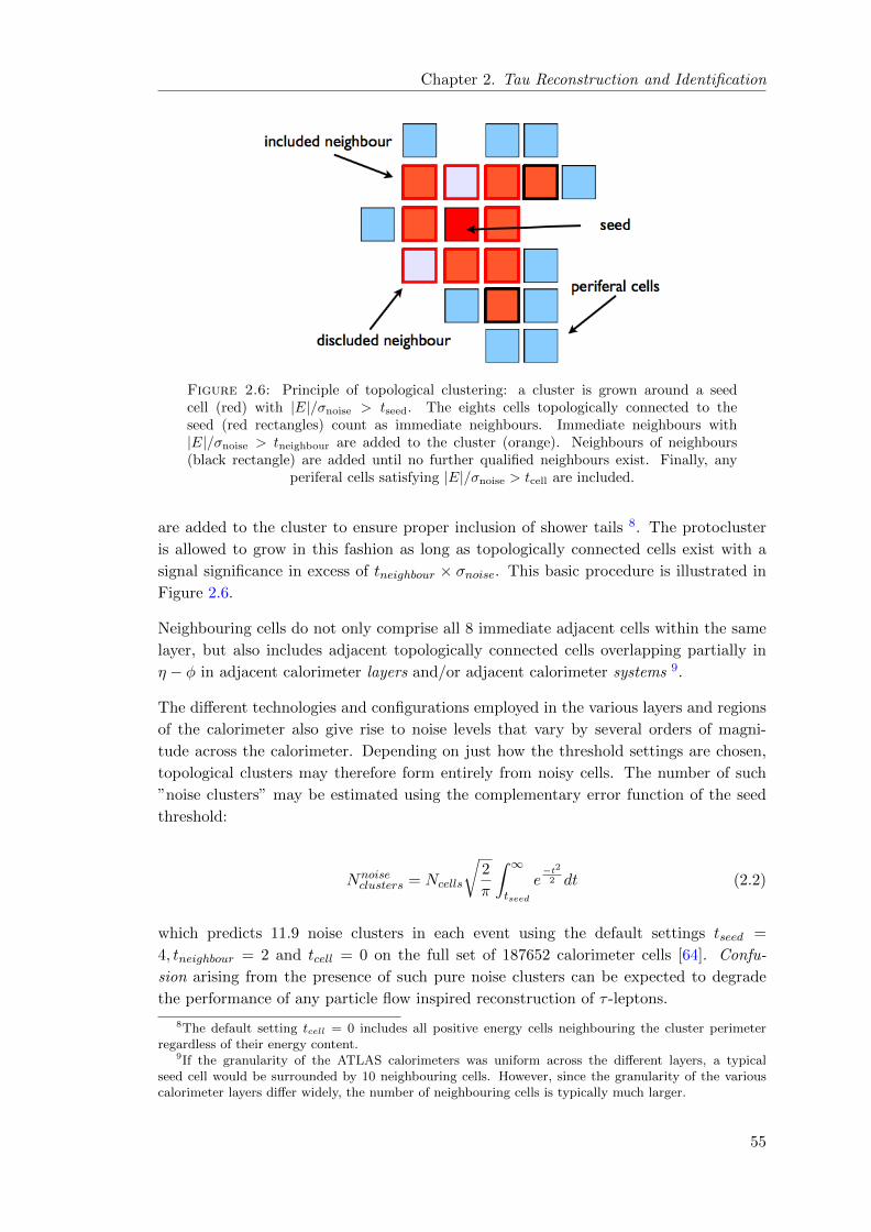
Chapter 2. Tau Reconstruction and Identification
Figure 2.6: Principle of topological clustering: a cluster is grown around a seedcell (red) with |E|/σnoise > tseed. The eights cells topologically connected to theseed (red rectangles) count as immediate neighbours. Immediate neighbours with|E|/σnoise > tneighbour are added to the cluster (orange). Neighbours of neighbours(black rectangle) are added until no further qualified neighbours exist. Finally, any
periferal cells satisfying |E|/σnoise > tcell are included.
are added to the cluster to ensure proper inclusion of shower tails 8. The protocluster
is allowed to grow in this fashion as long as topologically connected cells exist with a
signal significance in excess of tneighbour × σnoise. This basic procedure is illustrated in
Figure 2.6.
Neighbouring cells do not only comprise all 8 immediate adjacent cells within the same
layer, but also includes adjacent topologically connected cells overlapping partially in
η − φ in adjacent calorimeter layers and/or adjacent calorimeter systems 9.
The different technologies and configurations employed in the various layers and regions
of the calorimeter also give rise to noise levels that vary by several orders of magni-
tude across the calorimeter. Depending on just how the threshold settings are chosen,
topological clusters may therefore form entirely from noisy cells. The number of such
”noise clusters” may be estimated using the complementary error function of the seed
threshold:
Nnoiseclusters = Ncells
√2
π
∫ ∞tseed
e−t2
2 dt (2.2)
which predicts 11.9 noise clusters in each event using the default settings tseed =
4, tneighbour = 2 and tcell = 0 on the full set of 187652 calorimeter cells [64]. Confu-
sion arising from the presence of such pure noise clusters can be expected to degrade
the performance of any particle flow inspired reconstruction of τ -leptons.
8The default setting tcell = 0 includes all positive energy cells neighbouring the cluster perimeterregardless of their energy content.
9If the granularity of the ATLAS calorimeters was uniform across the different layers, a typicalseed cell would be surrounded by 10 neighbouring cells. However, since the granularity of the variouscalorimeter layers differ widely, the number of neighbouring cells is typically much larger.
55

Chapter 2. Tau Reconstruction and Identification
Cluster Splitting
Ideally the topological clustering algorithm as described above should render a one-to-
one correspondence between cluster and isolated showering particle, however without
some measure to resolve overlapping showers, this correspondence is rarely achievable in
ATLAS. Overlapping showers result in part from showering particles in too close a sepa-
ration, but also from the granularity and configuration of the calorimeters. In the more
forward regions of the detector, the comparatively coarse granularity of the endcaps and
FCAL combined with the typically higher density of particle debris often result in very
large topological clusters. In order to remedy unwanted cluster growth from shower
overlaps, all primary topoclusters resulting from the aforementioned clustering proce-
dure are subjected to a splitting algorithm. The splitting algorithm seeks to separate
overlapping showering particles by identifying local maxima in the primary topoclusters.
A local maximum is defined as an energetic (E > 500 MeV) clustered cell with more
energy than any of its neighbouring cells, of which there needs to be a minimum of 4.
To suppress noise cluster formation, cells from the presampler are excluded from this
procedure, while cells from the the strips and the HCAL are only used if they do not
η−φ overlap with a primary local maximum. Consequently, hadronic topoclusters with
a significant energy deposits in the ECAL are likely to split along their electromagnetic
core, while hadronic clusters with small electromagnetic components may be separated,
if required, using the coarser maxima located in the HCAL.
It is noteworthy that this splitting procedure may have both desirable and undesirable
consequences. In the context of a physical τ -decay, the splitting procedure may in some
cases help resolve the shower overlap between a π± and a π0, while it in other cases may
divide a single cluster resulting from a π± with an early shower in the ECAL. These
issues will be touched upon in Section 2.3.2.3.
Once all local maxima have been located in the primary topoclusters, secondary topoclus-
ters are re-grown about the local maxima following the aforementioned prescription with
the key difference that only cells forming part of a primary cluster are used (rendering
the application of thresholds redundant) and no cluster merging takes place, so that
each resulting cluster will contain only one local maximum. If a cell is found to border
more than one proto-cluster, its energy is shared in a weighted fashion between the two
proto-clusters containing the two most energetic neighbours. Primary topoclusters in
which no local maxima were found are kept intact.
The final collection of topological clusters passed as input to the energy flow algorithm,
therefore contains a mixture of primary topoclusters and secondary topoclusters re-
grown about local maxima, some of which may share cells along the perimeter.
2.3.1.2 The application of topological clustering to τ-decays
Figure 2.7 shows the structure of the topological clusters produced in response to a rela-
tively soft τ → ντπ±π0 decay in the first three layers of the electromagnetic calorimeter.
A comparatively high granularity combined with intelligent clustering is seen to render
56
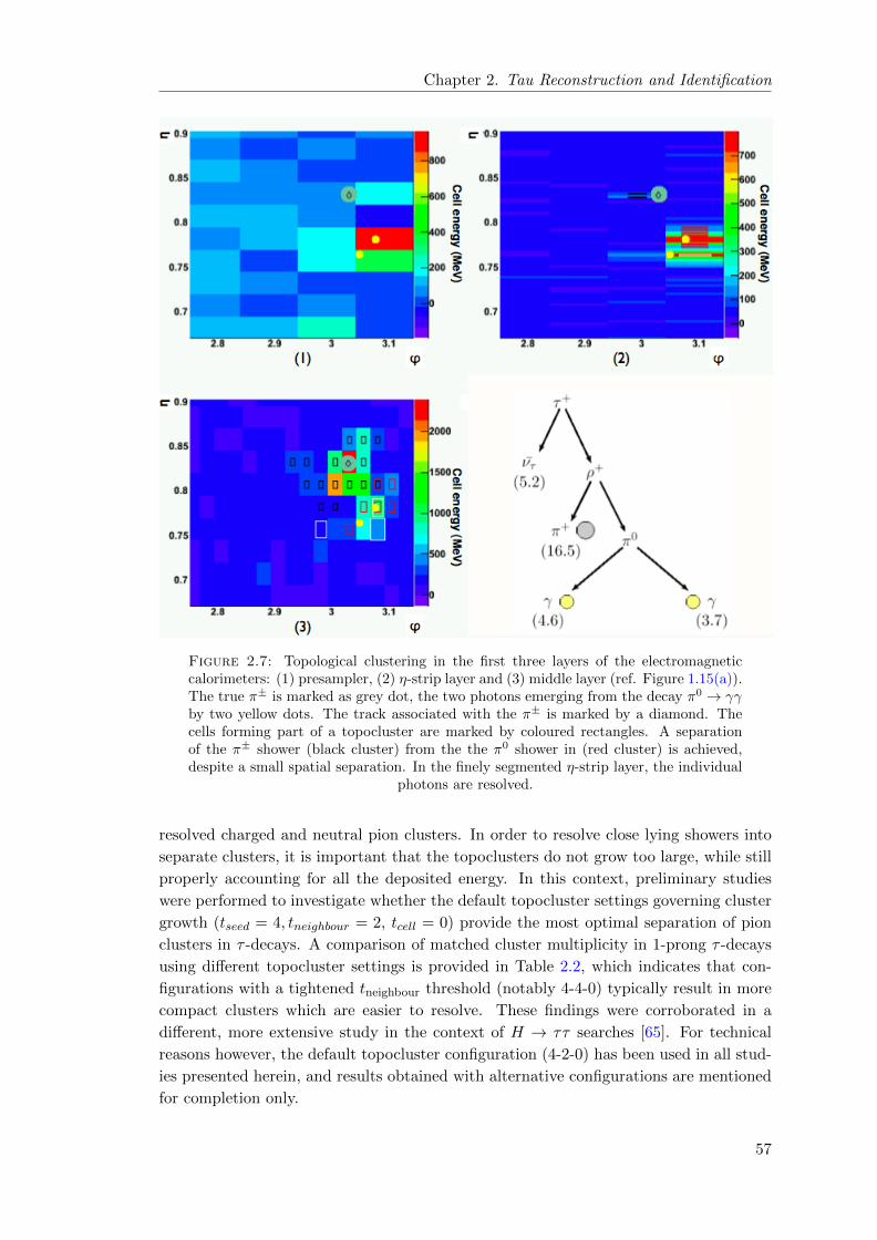
Chapter 2. Tau Reconstruction and Identification
Figure 2.7: Topological clustering in the first three layers of the electromagneticcalorimeters: (1) presampler, (2) η-strip layer and (3) middle layer (ref. Figure 1.15(a)).The true π± is marked as grey dot, the two photons emerging from the decay π0 → γγby two yellow dots. The track associated with the π± is marked by a diamond. Thecells forming part of a topocluster are marked by coloured rectangles. A separationof the π± shower (black cluster) from the the π0 shower in (red cluster) is achieved,despite a small spatial separation. In the finely segmented η-strip layer, the individual
photons are resolved.
resolved charged and neutral pion clusters. In order to resolve close lying showers into
separate clusters, it is important that the topoclusters do not grow too large, while still
properly accounting for all the deposited energy. In this context, preliminary studies
were performed to investigate whether the default topocluster settings governing cluster
growth (tseed = 4, tneighbour = 2, tcell = 0) provide the most optimal separation of pion
clusters in τ -decays. A comparison of matched cluster multiplicity in 1-prong τ -decays
using different topocluster settings is provided in Table 2.2, which indicates that con-
figurations with a tightened tneighbour threshold (notably 4-4-0) typically result in more
compact clusters which are easier to resolve. These findings were corroborated in a
different, more extensive study in the context of H → ττ searches [65]. For technical
reasons however, the default topocluster configuration (4-2-0) has been used in all stud-
ies presented herein, and results obtained with alternative configurations are mentioned
for completion only.
57

Chapter 2. Tau Reconstruction and Identification
Decay topology tseed − tneighbour − tcell 1 cluster 2 clusters 3 clusters
τ± → π±π0
4-4-0 11 % 89 % -4-3-0 14 % 86 % -4-2-0 20 % 80 % -5-5-0 11 % 89 % -5-4-0 13 % 87 % -6-6-0 12 % 88 % -6-5-0 13 % 87 % -
τ± → π±π0π0
4-4-0 3 % 24 % 73 %4-3-0 4 % 29 % 67%4-2-0 8 % 38 % 55%5-5-0 3 % 25 % 68%5-4-0 4 % 26 % 71%6-6-0 3 % 26 % 68%
Table 2.2: The fraction of events with reconstructed topoclusters matched to a truepion (∆R < 0.1) emerging from a decaying τ -lepton with 20 GeV< pvisT <25 GeV using
different topocluster configurations.
2.3.2 Energy flow in ATLAS
As indicated in Section 2.3, the merits of energy flow calorimetry depend in large part
on the accuracy with which energy deposits in the calorimeter can be associated with
the correct particles in the event. In practical terms, this necessitates the ability to
distinguish charged particle deposits in the calorimeter from neutral particle deposits, a
feature which may be achieved by matching reconstructed tracks to calorimeter clusters.
This is a relatively straightforward task in scenarios with well contained and isolated
calorimeter clusters corresponding to a few true particle energy deposits, but becomes
increasingly more complex as the separation between particle deposits become smaller.
If care is not taken, overlaps between charged and neutral showers may render part or
all of the neutral energy deposit lost after track momentum subtraction. Conversely,
if a hadronic shower is not fully contained in a single cluster, but split into multiple
clusters during reconstruction, the shower fragments without a track match are likely
to be falsely identified as additional neutral deposits and consequently the energy of the
showering particle is effectively double-counted.
Uncertainty of this sort is minimised by effective pattern recognition, provided in part by
granular calorimeters and efficient topological clustering, but equally important by ac-
curate track-cluster association and appropriate replacement of charged cluster deposits
in the calorimeter by track measurements.
A general ATLAS algorithm for the latter is provided by the eflowRec software package
[62, 66].
The input to eflowRec is a collection of tracks (TrackParticles) and a collection of
uncalibrated default (4-2-0) topological clusters (CaloTopoClusters). In a sequence of
steps, these objects are combined to form energy flow objects (EFOs) which may later
serve as input to particle reconstruction algorithms:
58
Chapter 2. Tau Reconstruction and Identification
1. Each track is extrapolated to the first layer of the electromagnetic calorimeter.
2. Using the extrapolated track coordinates, the nearest topological cluster is located.
3. The energy of the nearest cluster should agree with the expected energy deposit
Eexp(σexp) of the track match. Therefore, the closest cluster is required to satisfy:
Ecluster > Eexp − k2 × σexp
where Ecluster represents the cluster energy at the electromagnetic scale and Eexp
the expected electromagnetic scale energy deposit from a charged pion with the
energy and pseudorapidity corresponding to those of the track, as determined from
a reference sample. σexp represents the width of Eexp and k2 is a free parameter.
If the clusters satisfy the above condition, the expected energy deposit is removed
from the cluster:
E′cluster = Ecluster − Eexp.
This procedure is repeated for any other tracks matched to the same cluster.
4. After subtracting expected energy deposits from the cluster energy, any remaining
energy should ideally not originate from the particle(s) producing the track(s).
Therefore a final check is performed on the cluster:
E′cluster > k1 × σexp
where k1 is again a free parameter. If the condition is satisfied, the cluster is kept
and appropriate calibrations applied, otherwise the cluster is discarded.
2.3.2.1 Determining expected energy deposits
The expected energy deposits Eexp(σexp) are derived from reference samples of various
fixed energy single π±. Clusters are collected in a cone (∆R < 0.4) about the track
axis in the calorimeter, whereby the leading cluster is required to contain > 95% of the
energy in the cone and to be matched to the single pion track10. The expected energy
deposits are binned in track energy and pseudorapidity (and layer of first interaction in
the calorimeter).
2.3.2.2 Subtraction of energy deposits
The evolution of a hadronic cascade is chiefly characterized by a series of successive
inelastic hadronic interactions. While hadrons of various types are all produced as sec-
ondary particles, the particle content of the cascade is dominated by pions. Neutral
pions comprise roughly 1/3 of all pions produced in each inelastic interaction and these
will initiate electromagnetic subshowers inside the hadronic cascade. Because electro-
magnetic showers are comparatively well collimated, the electromagnetic component will
10The requirement on the cluster energy acts as a protection against showers split into several clusters.
59
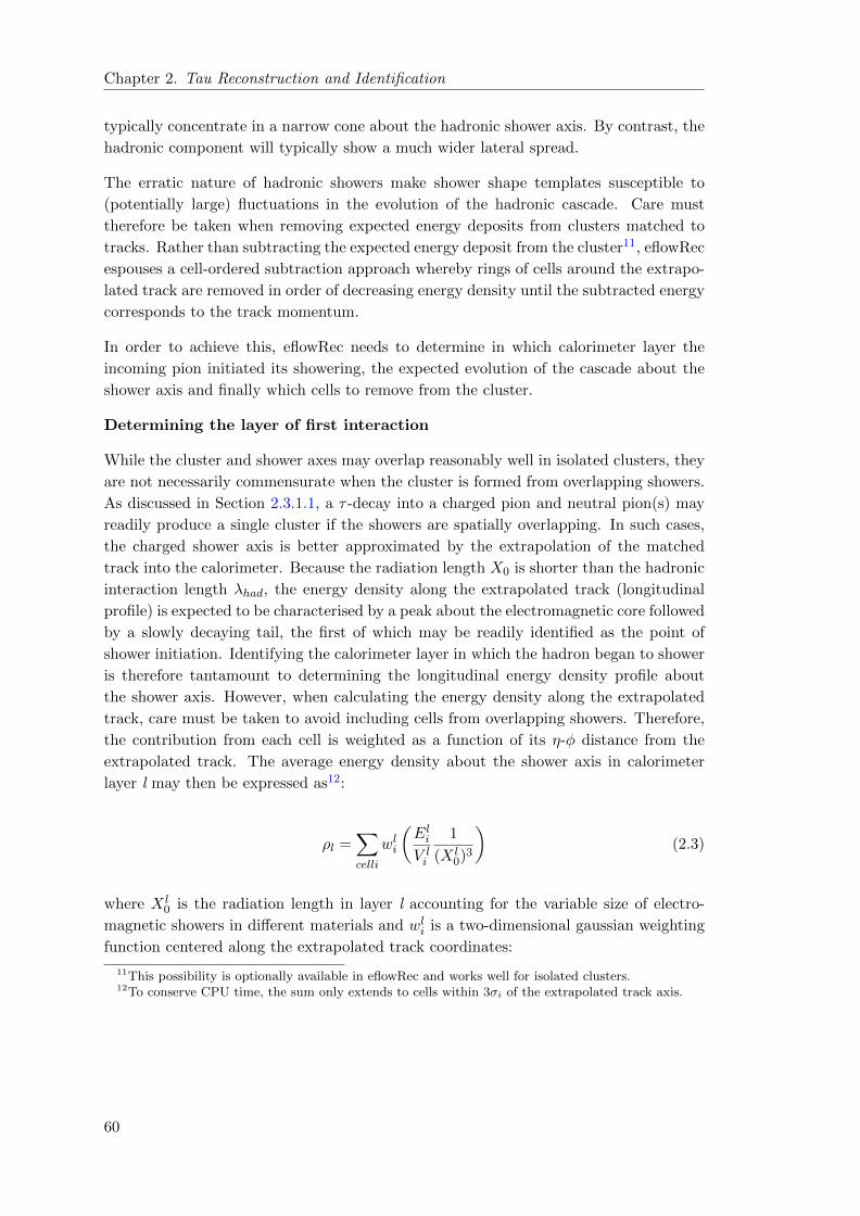
Chapter 2. Tau Reconstruction and Identification
typically concentrate in a narrow cone about the hadronic shower axis. By contrast, the
hadronic component will typically show a much wider lateral spread.
The erratic nature of hadronic showers make shower shape templates susceptible to
(potentially large) fluctuations in the evolution of the hadronic cascade. Care must
therefore be taken when removing expected energy deposits from clusters matched to
tracks. Rather than subtracting the expected energy deposit from the cluster11, eflowRec
espouses a cell-ordered subtraction approach whereby rings of cells around the extrapo-
lated track are removed in order of decreasing energy density until the subtracted energy
corresponds to the track momentum.
In order to achieve this, eflowRec needs to determine in which calorimeter layer the
incoming pion initiated its showering, the expected evolution of the cascade about the
shower axis and finally which cells to remove from the cluster.
Determining the layer of first interaction
While the cluster and shower axes may overlap reasonably well in isolated clusters, they
are not necessarily commensurate when the cluster is formed from overlapping showers.
As discussed in Section 2.3.1.1, a τ -decay into a charged pion and neutral pion(s) may
readily produce a single cluster if the showers are spatially overlapping. In such cases,
the charged shower axis is better approximated by the extrapolation of the matched
track into the calorimeter. Because the radiation length X0 is shorter than the hadronic
interaction length λhad, the energy density along the extrapolated track (longitudinal
profile) is expected to be characterised by a peak about the electromagnetic core followed
by a slowly decaying tail, the first of which may be readily identified as the point of
shower initiation. Identifying the calorimeter layer in which the hadron began to shower
is therefore tantamount to determining the longitudinal energy density profile about
the shower axis. However, when calculating the energy density along the extrapolated
track, care must be taken to avoid including cells from overlapping showers. Therefore,
the contribution from each cell is weighted as a function of its η-φ distance from the
extrapolated track. The average energy density about the shower axis in calorimeter
layer l may then be expressed as12:
ρl =∑celli
wli
(EliV li
1
(X l0)3
)(2.3)
where X l0 is the radiation length in layer l accounting for the variable size of electro-
magnetic showers in different materials and wli is a two-dimensional gaussian weighting
function centered along the extrapolated track coordinates:
11This possibility is optionally available in eflowRec and works well for isolated clusters.12To conserve CPU time, the sum only extends to cells within 3σi of the extrapolated track axis.
60

Chapter 2. Tau Reconstruction and Identification
wli =
∫ ∫celli
gli(η, φ)dηdφ (2.4)
=1
2πσ2l
∫ ∫exp
((ηi − ηtrkp )2 + (φi − φtrkl )2
2σ2i
)dηdφ (2.5)
Finally, the longitudinal profile (energy density in each layer) may be expressed as a
function of calorimeter depth measured in interaction lengths λhad:
Pl =< ρ >l − < ρ >l−1
< λ >l − < λ >l−1(2.6)
and the layer of first interaction defined as the calorimeter layer preceding the largest
gradient of this profile.
Radial shower shapes and cell ordering
Once the starting point of the shower to which the track is matched is identified, a
method is called for by which the relevant cells along the extrapolated track are removed.
Since hadronic cascades are prone to fluctuate considerably, mean shower shapes will
necessarily be inaccurate. Because the electromagnetic core is more predictable and
contains the majority of the shower energy concentrated along the shower axis, the
energy density provides a viable order for cell subtraction. The stability of this region
with respect to variations in lateral spread allows one to assume a radially symmetric
profile about the extrapolated track13. Assuming radial symmetry, the radial energy
density profile may be computed in each layer. For a reference sample of single charged
pions of a given energy E, η and shower initiation in calorimeter layer l, cells about the
track are binned in radial distance from the extrapolated track axis to form rings of
thickness ∆Rl = 12
√(∆ηl)2 + (∆φl)2 ,where ∆ηl and ∆φl represent the cell dimensions
in calorimeter layer l. The rings in all layers are then ordered in energy density to
provide the overall order in which cells can be removed from the matched cluster.
In summary, the entire cell subtraction process therefore amounts to executing the fol-
lowing steps on all matched tracks in order of descending pT :
1. Determine the layer of first interaction in the matched cluster and retrieve the
appropriate ordering as defined by the track energy and η and the layer of first
interaction.
2. For each layer in the matched cluster, order cells by radial distance from the
extrapolated track coordinates and order the resulting ”cell rings” according to
the ordering scheme derived in (1).
3. Subtract rings of cells in order of decreasing energy density until ptrack has been
removed.13The validity of this assumption may be increasingly challenged as one moves away from the core of
the shower.
61
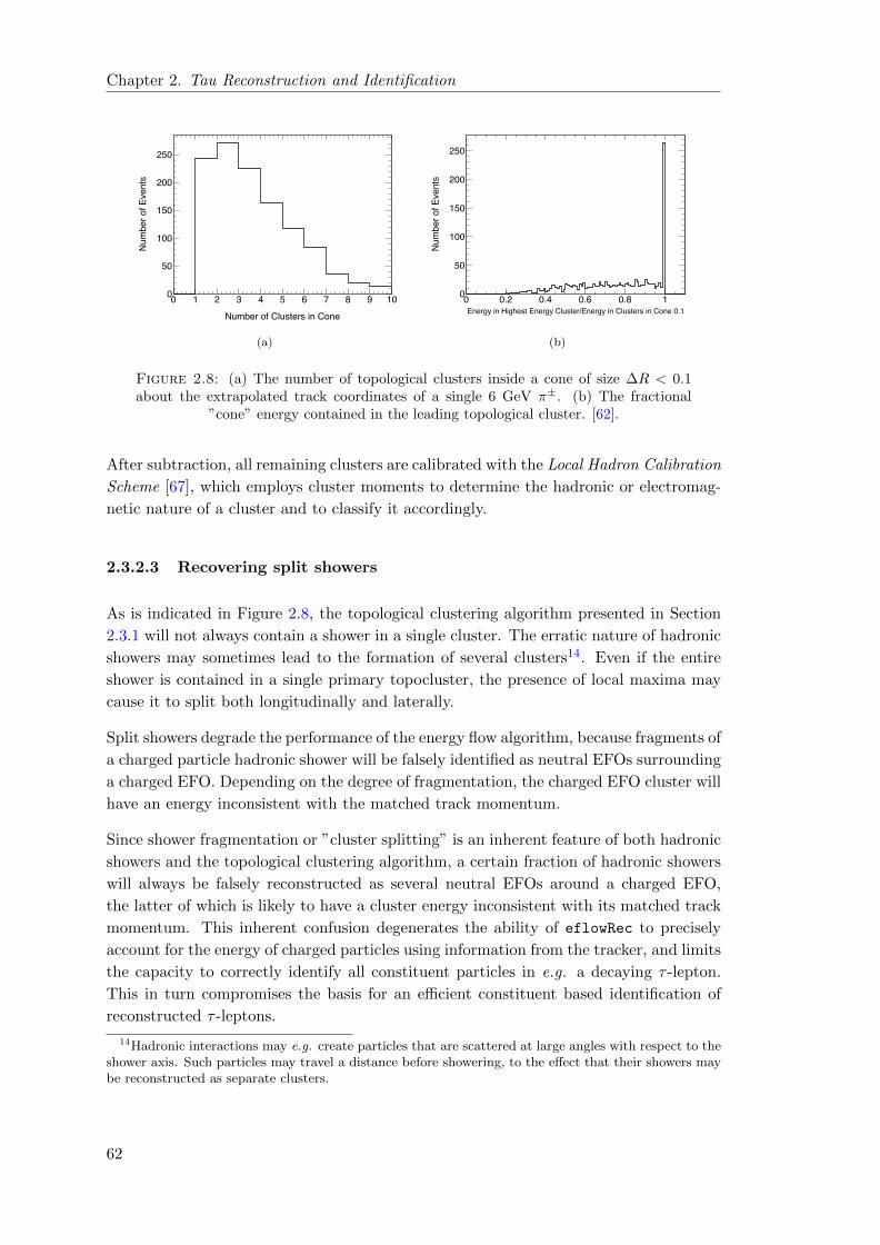
Chapter 2. Tau Reconstruction and Identification
Number of Clusters in Cone0 1 2 3 4 5 6 7 8 9 10
Num
ber o
f Eve
nts
0
50
100
150
200
250
(a)
Energy in Highest Energy Cluster/Energy in Clusters in Cone 0.10 0.2 0.4 0.6 0.8 1
Num
ber o
f Eve
nts
0
50
100
150
200
250
(b)
Figure 2.8: (a) The number of topological clusters inside a cone of size ∆R < 0.1about the extrapolated track coordinates of a single 6 GeV π±. (b) The fractional
”cone” energy contained in the leading topological cluster. [62].
After subtraction, all remaining clusters are calibrated with the Local Hadron Calibration
Scheme [67], which employs cluster moments to determine the hadronic or electromag-
netic nature of a cluster and to classify it accordingly.
2.3.2.3 Recovering split showers
As is indicated in Figure 2.8, the topological clustering algorithm presented in Section
2.3.1 will not always contain a shower in a single cluster. The erratic nature of hadronic
showers may sometimes lead to the formation of several clusters14. Even if the entire
shower is contained in a single primary topocluster, the presence of local maxima may
cause it to split both longitudinally and laterally.
Split showers degrade the performance of the energy flow algorithm, because fragments of
a charged particle hadronic shower will be falsely identified as neutral EFOs surrounding
a charged EFO. Depending on the degree of fragmentation, the charged EFO cluster will
have an energy inconsistent with the matched track momentum.
Since shower fragmentation or ”cluster splitting” is an inherent feature of both hadronic
showers and the topological clustering algorithm, a certain fraction of hadronic showers
will always be falsely reconstructed as several neutral EFOs around a charged EFO,
the latter of which is likely to have a cluster energy inconsistent with its matched track
momentum. This inherent confusion degenerates the ability of eflowRec to precisely
account for the energy of charged particles using information from the tracker, and limits
the capacity to correctly identify all constituent particles in e.g. a decaying τ -lepton.
This in turn compromises the basis for an efficient constituent based identification of
reconstructed τ -leptons.
14Hadronic interactions may e.g. create particles that are scattered at large angles with respect to theshower axis. Such particles may travel a distance before showering, to the effect that their showers maybe reconstructed as separate clusters.
62

Chapter 2. Tau Reconstruction and Identification
In order to counter any performance degradation resulting from cluster splitting, an
attempt is made to recover fragmented showers by re-associating additional neutral
EFOs with the appropriate parent charged EFO:
(i) Identify all charged EFOs whose associated cluster energy is found to be inconsis-
tent with the expected charged deposit as determined by the matched track (and
optionally also any EFOs for which no cluster match was found).
(ii) Build a cone ∆R < 0.2 around the extrapolated track axis.
(iii) Subtract the expected charged energy deposit from any neutral EFO (topoclusters)
whose barycenter is located inside this cone.
(iv) Calibrate any remaining neutral EFOs using the Local Hadron Calibration scheme.
Despite the simplicity of the recovery algorithm described above, Figure 2.9 shows that
it provides a good working performance, correcting for the large majority of cases
where charged pion showers fragment into multiple EFOs. While not run by default
in eflowRec, the recovery algorithm has therefore been applied to all results presented
herein.
2.3.2.4 Applications to tau reconstruction
With the potential to access the substructure of (hadronic) τ -decays using the ATLAS
calorimeters, it is germane to consider the potential benefits of applying generic energy
flow techniques at an early stage in the τ -reconstruction. Figure 2.10 compares the
transverse energy resolutions obtained in τ± → ρ± → π±π0 and τ± → a±1 → π±π0π0
decays using only calibrated topological clusters and using EFOs. Improvements of 19%
and 5%, respectively are found in case of the latter. These improvements currently
come at the cost of an energy scale overestimation of 4%, to be compared with an
underestimation of 0.5% using only topological clusters [62]. (It has also been established
that the reconstructed ρ-mass distributions have notably fatter right-sided tails. At the
time of writing this bias is not understood and under investigation[68]).
2.4 PanTau - particle flow inspired τ-reconstruction
The two canonical approaches to τ -lepton reconstruction and identification in ATLAS
were described in Section 2.2. In what follows, an entirely different approach to τ -
reconstruction will be discussed in the context of a newly developed τ -reconstruction
algorithm for ATLAS, known as PanTau15.
15PanTau (Particle Analysis of Taus) is named after a character by the same name in a Czech/Germanchildren’s television series from the late 1960s and 1970s, known for his magic bowler hat.
63

Chapter 2. Tau Reconstruction and Identification
Reconstructed Et/True Visible Et0 0.2 0.4 0.6 0.8 1 1.2 1.4 1.6 1.8 2
Num
ber o
f Eve
nts
0
20
40
60
80
100
120 0.004±<> = 1.002 0.006± = 0.098 !
(a) τ± → π±ντ , no recovery
Reconstructed Et/True Visible Et0 0.2 0.4 0.6 0.8 1 1.2 1.4 1.6 1.8 2
Num
ber o
f Eve
nts
0
50
100
150
200
250
300
350 0.001±<> = 1.005
0.002± = 0.031 !
(b) τ± → π±ντ , with recovery
Reconstructed Charged ET/Visible Charged ET0 0.2 0.4 0.6 0.8 1 1.2 1.4 1.6 1.8 2
Num
ber o
f Eve
nts
0
50
100
150
200
250
300
(c) τ± → ρ±ντ → π±π0ντ , no recovery
Reconstructed Charged ET/Visible Charged ET0 0.2 0.4 0.6 0.8 1 1.2 1.4 1.6 1.8 2
Num
ber o
f Eve
nts
0
100
200
300
400
500
(d) τ± → ρ±ντ → π±π0ντ , with recovery
Figure 2.9: Transverse energy resolutions with and without the split cluster recoveryalgorithm. The resolutions are calculated using all EFOs in a cone of size ∆R < 0.2
about the charged EFO [62].
This work is the result of a joint effort with Sebastian Fleischmann, with whom all
credit is shared16. Important contributions have also been made by Christian Limbach
and Peter Wienemann. The invaluable support and close cooperation with eflowRec-
author Mark Hodgkinson is also gratefully acknowledged.
2.4.1 The philosophy of PanTau
Inspired by the ideas of particle flow, PanTau aims to identify τ -leptons by way of their
resolved constituent decay particles. Rather than approaching the hadronic decay of a
τ -lepton as a narrow jet in the detector, PanTau seeks to recognize decay topologies
consistent with a hadronically decaying τ using information from resolved ”particles” in
its decay wake. Any potential decay information provided by the topological clustering
of calorimeter cells is harnessed through the exclusive use of EFOs provided by the
eflowRec algorithm. These EFOs form the base units of operation in the algorithm,
under the assumption that they mirror the particle content of the τ -lepton decay and
that most observable properties of the τ -lepton can be derived from these objects alone.
16The authour retains responsibility for any errors, omissions or misgivings in the text.
64

Chapter 2. Tau Reconstruction and Identification
Reconstructed Et/True Visible Et0 0.2 0.4 0.6 0.8 1 1.2 1.4 1.6 1.8 2
Num
ber o
f Eve
nts
0
20
40
60
80
100
120
140
160 0.003±<> = 0.996
0.004± = 0.095 !
(a) τ± → ρ±ντ → π±π0ντ (Topological clusters)
Reconstructed Et/True Visible Et0 0.2 0.4 0.6 0.8 1 1.2 1.4 1.6 1.8 2
Num
ber o
f Eve
nts
020406080
100120140160180 0.003±<> = 1.043
0.003± = 0.080 !
(b) τ± → ρ±ντ → π±π0ντ (Energy flow objects)
Reconstructed Et/True Visible Et0 0.2 0.4 0.6 0.8 1 1.2 1.4 1.6 1.8 2
Num
ber o
f Eve
nts
0
10
20
30
40
50
60
70 0.005±<> = 0.982
0.006± = 0.095 !
(c) τ± → a±1 ντ → π±π0π0ντ (Topological clusters)
Reconstructed Et/True Visible Et0 0.2 0.4 0.6 0.8 1 1.2 1.4 1.6 1.8 2
Num
ber o
f Eve
nts
0
10
20
30
40
50
60
70
80
90 0.005±<> = 1.039
0.007± = 0.095 !
(d) τ± → a±1 ντ → π±π0π0ντ , (Energy flow objects)
Figure 2.10: A comparison of transverse energy resolutions obtained with calibratedtopoclusters (left) and EFOs (right) in 1-prong τ -decays with additional neutrals [62]
Rather than explicitly drawing on information from the detector (such as e.g. the
number of hits in the η-strip layers of the calorimeter or the transverse shower profile
of the τ -jet), the aim throughout is to rely squarely on the use of constituent EFOs to
identify signatures deemed compatible with a physical τ -decay in a manner dissociated
from the details of the underlying detector configuration.
As such, PanTau elicits a natural separation between the physics of the τ -lepton decay
and any detector effects that are sensitive the underlying technology. It is hoped that
this separation, combined with an increasingly modular approach to the combined re-
construction of τ -leptons, may facilitate an improved interpretation of data and a better
understanding of effects that may impact traditional τ -reconstruction tools in ATLAS.
2.4.2 General overview
The overall structure of PanTau is illustrated in the flow chart depicted in Figure 2.11.
The details of the implementation of the this software into the ATLAS software frame-
work ATHENA is detailed elsewhere [69]. Here, only a qualitative description of the
structure of the algorithm will be given with aim to highlight any departures from de-
fault τ -reconstruction in ATLAS. Moreover, this document will only concern itself with
65

Chapter 2. Tau Reconstruction and Identification
the reconstruction of hadronically decaying τ -leptons. The reconstruction of leptonically
decaying τ -leptons within the framework of PanTau is described in [48].
I Input
The raw input to PanTau are EFOs provided by the eflowRec algorithm described in
Section 2.3.2.
In order to identify objects corresponding to a τ decay, some measure must be provided
by which the relevant EFOs are collected and passed to PanTau for inspection. The
simplest (if not necessarily always the best) method of collecting the relevant EFOs is
by way of jet algorithms made to run on all EFOs in a given event.
II Seed selection & classification
These jets serve as seeds for the PanTau algorithm. Each seed is scanned to determine its
composition through a simple count of its constituent charged and neutral EFOs. Seeds
whose composition is found to be inconsistent with the expected particle configuration
of a τ decay (e.g. seeds containing 8 charged EFOs) can therefore be discarded early.
Seeds with a composition compatible with a τ decay are categorized according to their
”particle content”. In this manner, seeds with e.g. one charged EFO and one or more
neutral EFO(s) can be classified as τvis → π± + nπ0 candidate decays, whereas seeds
with e.g. three charged EFOs and no neutral EFOs are classified as τvis → π+π−π+
candidates. As such, the constituent composition of the input seeds provides both a
rough discrimination against false candidates, as well as an estimate of the most probable
decay mode of the τ -lepton candidate. It also follows that any remaining seeds that do
not originate from a true τ decay but still pass the initial selection are likely to greatly
resemble a true τ decay and will be challenging to separate from true τ -leptons.
III Feature determination
Following the comparatively simple classification of seeds, more involved quantities de-
rived from the constituent objects are computed. These quantities, henceforth called
features, provide the basis for the separation of τ -induced seeds from jet-induced seeds.
Unlike the discriminating variables used in the τ -reconstruction algorithms described in
Section 2.2, the seed features all derive squarely from the system of constituent EFOs
and the EFOs themselves. No information is drawn directly from the calorimeter or
tracker.
IV Kinematic fit
Seeds classified as compatible with a τvis → π±+nπ0 decay may optionally be subjected
to a kinematic fit, constrained by the masses and widths of the ρ and a1 resonances.
(At the time of writing, this method is still in a testing phase and will therefore not be
discussed further herein. It is mentioned here for completion only).
V Multivariate discrimination
Several seed features may be combined into a multivariate discriminant to enhance
signal identification efficiency and background suppression. The most appropriate suite
66

Chapter 2. Tau Reconstruction and Identification
Energy flow objects
Jet algorithm onenergy flow objects
PreselectionRejectseed
Seed classification
3-prongw/
neutral
3-prong1-prong
w/neutral
1-prong 2-prong2-prong
w/neutral
Not a τ
Feature determination
Kinematic fit
Multivariatediscrimination
Tau jet building
Figure 2.11: Data flow in PanTau: EFOs form the raw input to the algorithm. Theseare collected by a jet algorithm to form τ -seeds. The seeds are subsequently classifiedaccording to content, if found to satisfy a basic preselection. (Seeds classified as 2-prong or 2-prong w/neutral have two EFO±q .) After classification, properties of theseeds are derived from the constituent objects and fed into a multivariate discriminant
to facilitate the separation of QCD-induced fakes.
67

Chapter 2. Tau Reconstruction and Identification
Category Classification requirements
1-prong 1 EFO±q and absence of neutral energy
1-prong+neutral 1 EFO±q and presence of neutral energy
3-prong 3 or 4 EFO±q and absence of neutral energy
3-prong+neutral 3 or 4 EFO±q and presence of neutral energy
2-prong 2 EFO±q and absence of neutral energy
2-prong+neutral 2 EFO±q and presence of neutral energy
Other 0 or > 4 EFO±q or otherwise failing alternative classification
Table 2.3: The PanTau seed classification scheme.
of features to combine will vary according to the characteristics of each seed category.
The multivariate training is therefore performed separately in each category.
VI Tau-object building
The final step involves the building of a τ -object intended for use in an offline analysis,
with all associated properties as estimated by previous steps in the algorithm.
In the following, a more elaborate discussion of the details pertaining to steps II, III
and V above is provided.
2.4.3 Seeding
With the input EFOs scattered across the detector, some association measure is required
by which relevant systems of EFOs are identified, collected and passed on to PanTau for
closer inspection. In this context, jet algorithms provide a simple method of gathering
all EFOs that may be relevant to the identification of a τ -decay. The resulting jets may
then act as seeds for the τ -reconstruction. Unless stated otherwise, fixed size ∆R = 0.4
cone jets (ref. Section 4.4.4) built on default EFOs have acted as seeds for all results
presented herein. The drawbacks of this approach are discussed below in Section 2.4.3.2.
After an initial scan of its constituent composition, the seed is retained if accepted by a
rough pre-selection designed to enable an early rejection of seeds whose EFO-composition
is plainly incompatible with a hadronically decaying τ -lepton:
1. |EFO∑
Charge| > 0 and |EFO∑
Charge| ≤ 5
2. 0 < NEFO± ≤ 4
3. |ηseed| ≤ 2.7
Seeds passing the minimal preselection are subsequently classified into seven different
categories in accordance with their ”particle content” as detailed in Table 2.3.
In order to facilitate a more accurate classification, the track selection on charged EFOs
is moderately tightened with respect to the default track selection applied in eflowRec.
68

Chapter 2. Tau Reconstruction and Identification
Charged EFOs whose associated tracks satisfy these criteria are henceforth referred to
as charged qualified and labelled EFO±q . An EM neutral EFO is defined as an EFO with
ET > 1 GeV whose associated cluster has not been tagged as hadronic (HAD) by the
Local Hadron Calibration scheme. All considered EFOs are further subjected to a pion
mass hypothesis, whereby their 4-vectors are corrected for the charged or neutral pion
mass.
The presence of neutral energy in the seed is defined by way of the ratio
∑neutral EFO
EEFOT∑
charged EFO
EEFOT
(2.7)
which if found to be smaller than 0.3, qualifies the seed for the appropriate X-prong (w/o
neutrals) category. Otherwise the seed will qualify for an appropriate X-prong+neutral
category provided it does not contain an excess of hadronic neutral transverse energy:
∑HAD neutral EFO
EEFOT∑
all EFO
EEFOT
< 0.4 (2.8)
Seeds failing condition 2.8 will be classified as Other, indicating an inconsistency with the
expected composition of a hadronically decaying τ -lepton, unless the leading hadronic
neutral EFO accounts for a sizeable fraction of the total neutral energy in the seed:
Eleading HAD neutral EFOT ∑
neutral EFO
EEFOT
> 0.4 (2.9)
and the total number of charged EFOs (qualified and unqualified) remains low
NEFO± < 4 (2.10)
The latter requirements protects against cases where EM neutral energy in τ -induced
seeds is falsely tagged as hadronic.
2.4.3.1 Seed classification performance
The performance of the classification scheme described above is shown in Figures 2.12
and 2.13, in which the distribution of τ -induced seeds (seeds matched to a true τ) and
jet-induced seeds (seeds for which no match to a true τ was found) across the different
classification categories is detailed.
69
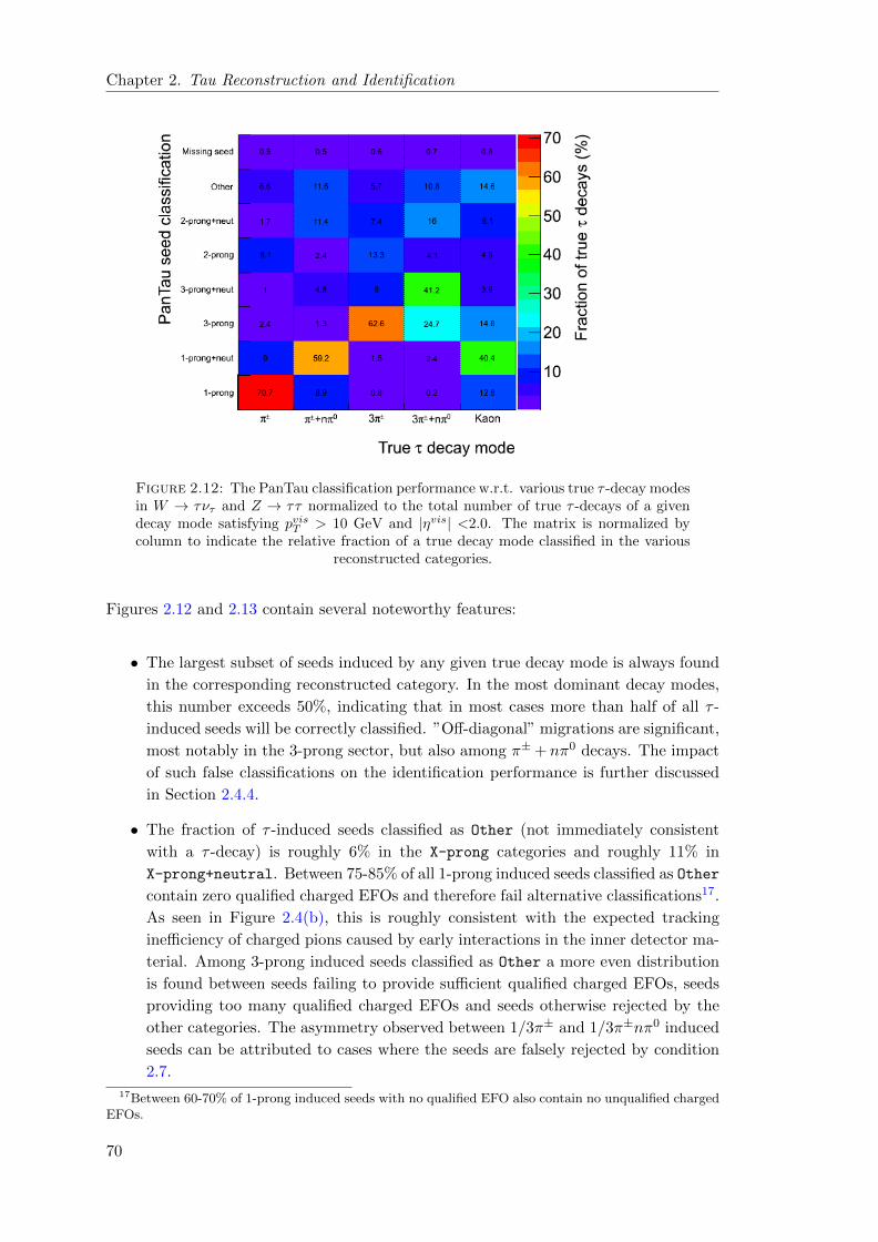
Chapter 2. Tau Reconstruction and Identification
Figure 2.12: The PanTau classification performance w.r.t. various true τ -decay modesin W → τντ and Z → ττ normalized to the total number of true τ -decays of a givendecay mode satisfying pvisT > 10 GeV and |ηvis| <2.0. The matrix is normalized bycolumn to indicate the relative fraction of a true decay mode classified in the various
reconstructed categories.
Figures 2.12 and 2.13 contain several noteworthy features:
• The largest subset of seeds induced by any given true decay mode is always found
in the corresponding reconstructed category. In the most dominant decay modes,
this number exceeds 50%, indicating that in most cases more than half of all τ -
induced seeds will be correctly classified. ”Off-diagonal” migrations are significant,
most notably in the 3-prong sector, but also among π±+nπ0 decays. The impact
of such false classifications on the identification performance is further discussed
in Section 2.4.4.
• The fraction of τ -induced seeds classified as Other (not immediately consistent
with a τ -decay) is roughly 6% in the X-prong categories and roughly 11% in
X-prong+neutral. Between 75-85% of all 1-prong induced seeds classified as Other
contain zero qualified charged EFOs and therefore fail alternative classifications17.
As seen in Figure 2.4(b), this is roughly consistent with the expected tracking
inefficiency of charged pions caused by early interactions in the inner detector ma-
terial. Among 3-prong induced seeds classified as Other a more even distribution
is found between seeds failing to provide sufficient qualified charged EFOs, seeds
providing too many qualified charged EFOs and seeds otherwise rejected by the
other categories. The asymmetry observed between 1/3π± and 1/3π±nπ0 induced
seeds can be attributed to cases where the seeds are falsely rejected by condition
2.7.
17Between 60-70% of 1-prong induced seeds with no qualified EFO also contain no unqualified chargedEFOs.
70

Chapter 2. Tau Reconstruction and Identification
Figure 2.13: The distribution of jet-induced seeds (fakes) from various samples acrossthe different PanTau classification categories normalized to the number of jet-induced
seeds in each sample satisfying seed pT > 10 GeV and seed |η| < 2.0.
• In all τ -decay modes, a small fraction (∼ 0.5%) of decays fail to produce an
adequately matched seed. Entries in the Missing Seed category shown in Figure
2.12 typically correspond to τ -decays of comparatively low visible momenta (< 15
GeV).
• A significant fraction (∼ 30− 60%) of jet-induced seeds are immediately classified
as Other. The remainder are largely distributed across the X-prong+neutral cat-
egories, most notably 3-prong+neutral. The fraction of jet-induced seeds falsely
classified in an X-prong category is small by comparison and does not exceed a few
percent in either category. It naturally follows that jet-induced seeds falsely asso-
ciated with any X-prong(+neutral) category will significantly resemble τ -induced
seeds classified in the same category.
2.4.3.2 A note on the choice of jet algorithm
As described above, the primary purpose of the seed jet is to collect and associate EFOs
that may originate from a τ -decay. The substructure of the seed jet is subsequently
probed to determine whether the seed composition is compatible with a hadronic τ -
decay or not. While the choice of the underlying jet algorithm used to produce the seed
jets is arbitrary, the seeding performance will necessarily depend on the details of the
algorithm that govern which EFOs to associate with a seed jet and which to exclude.
Ideally the collection process should be such that only EFOs associated with the seed
producing particle are contained in the resulting seed jet. The drawbacks of a fixed-sized
cone approach are apparent: a large cone size runs the risk of including unassociated
71

Chapter 2. Tau Reconstruction and Identification
EFOs, whereas a small cone size may exclude relevant EFOs. Either case may result in
either an incorrect classification and/or a reduced identification performance.
Moreover, the appropriate cone size will depend on the energy and showering properties
of the seed producing particle. The distance between constituent objects of a τ -lepton
decay may be comparatively large at low transverse momenta and considerably smaller
at higher momenta. While a narrow cone (∆R ∼ 0.2) is arguably more suitable for the
collection of τ -decay constituents beyond the very low-pT regime, it is likely to grossly
underestimate the true composition of jet-induced seeds from quarks and gluons, artifi-
cially making them appear more τ -like. To avoid unwanted truncations, a comparatively
broad cone (∆R = 0.4) has been used in the studies presented herein.
While a wide cone approach may have its merits in event topologies were the τ -leptons
are relatively isolated, it is arguably more problematic in busy environments where close-
lying unassociated EFOs may be included in the seed jet. Furthermore, a jet-based
approach to seeding is only justified whenever a τ -decay results in several EFOs. In
decay modes such as τ → π±ντ , in which only one EFO is expected, a jet-based seeding
is no longer warranted. Alternative seeding methods are therefore being explored.
2.4.4 Discrimination against QCD jets
While a decent fraction of jet-induced seeds are seen to be filtered away during seed
classification, the various X-prong(+neutral) categories still remain ”contaminated” by
a significant fraction of falsely classified jet-induced seeds. The base composition of these
jet-induced seeds is likely to greatly resemble that of their τ−induced counterparts. In
order to separate τ -induced seeds in a given category from falsely classified jet-induced
seeds, it is necessary to identify properties of either seed type that enable an efficient
differentiation. For an enhanced separation, several such characteristic seed features
can be combined in various multivariate discriminants. The most appropriate choice of
features to combine will often depend on the comparative characteristics of the signal
(τ -induced seeds) and background (jet-induced seeds) in each classification category18.
The most appropriate feature suite will also depend on the background composition (e.g.
gluon jets vs. quark jets) in a given category and their relative contributions in different
kinematic regimes.
2.4.4.1 The relative composition of the signal within categories
An accurate prediction of the expected appearance of τ -induced seeds in a given cate-
gory is a helpful tool to facilitate a separation from jet-induced seeds wrongly classified
in the same category. To enable such a prediction, it is desirable to keep the fraction of
τ -induced seeds from the target decay as high as possible and to minimize any ”contam-
ination” from unwanted off-diagonal migrations. The impact of off-diagonal migrations
18Some features are only properly defined if the seed constituents satisfy some base criteria, e.g. thatthe seed contains a certain number of EFOs of a given type.
72

Chapter 2. Tau Reconstruction and Identification
Figure 2.14: Fractional composition (”purity”) of each PanTau classification categorywith respect to true τ -decays from W → τντ and Z → ττ satisfying seed pT > 10GeV and seed |η| < 2.0. The matrix is normalized by row to indicate the relative
contributions from the various true decay modes in each reconstructed category.
are seen in Figure 2.14 in which the fractional population of various true decay modes
in each reconstructed classification category is shown.
While the categories 1-prong+neutral and 3-prong are notably ”clean” with the ma-
jority contribution originating from the target decay process, large admixtures are seen
in all other reconstructed categories. Significant ”contamination” from falsely classi-
fied π± + nπ0 decays are seen in both 1-prong and 3-prong+neutral categories. The
2-prong category receives roughly equal contributions from 1-prong and 3-prong de-
cays, whereas the 2-prong+neutral category is more dominated by π± + nπ0 decays.
(Kaon decays are seen to distribute themselves more evenly across the different cate-
gories). Large spreads between decay modes, such as those seen in the 3-prong+neutral
and 2-prong categories makes it more difficult to identify unique features to separate
τ -induced seeds from jet-induced seeds.
2.4.4.2 The pT dependence of the classification of fakes
As discussed in Section 2.1.3, the most prolific source of jet-induced seeds at the LHC
is arguably QCD jet production involving a hard scatter between two coloured parti-
cles. Such processes will often be accompanied by (comparatively soft) gluon radiation
both before and after the hard scattering. Jet-induced seeds may arise from both hard
scattered particles and radiated gluons, and the resulting seeds will typically distribute
themselves unevenly across the various PanTau classification categories. As seen in Fig-
ure 2.15, jet-induced seeds originating from comparatively soft gluon emissions are seen
to dominate the background in nearly all classification categories in the lower kinematic
73

Chapter 2. Tau Reconstruction and Identification
(a) (b)
Figure 2.15: Transverse momentum distribution of jet-induced seeds from QCD inthe various classification categories: (a) normalized to the respective total number offake seeds in each category, (b) normalized to the total number of fake seeds of a given
transverse momentum.
region (< 20 GeV). At higher transverse momenta, jet-induced seeds are seen to be
more readily classified as Other or 3-prong+neutral and are consequently less likely to
contribute to the fake contamination of any other category. This strong pT -dependence
is particularly visible in the 1-prong categories, and may illicit the use of different sets of
discriminating variables at low transverse momenta and at higher transverse momenta.
2.4.4.3 Feature classes and feature definitions
In line with the philosophy of PanTau, all seed features are constructed squarely from
the constituent ”particles” (EFOs) found in the input seeds. As the EFOs form the base
unit of all discriminating features, information from the tracker and calorimeters is only
drawn upon in an indirect manner. A large number of features with varying degrees of
discriminating power have been implemented in PanTau which may be broadly organized
in seven different feature classes. Rather than providing a detailed listing of all available
features, examples from either feature class are highlighted below. Distributions for
these features in the various categories are shown in succeeding section.
Class 1: Seed object composition
Even after seed classification, differences in the relative multiplicities of EFOs of a given
type are typically observable between τ -induced and jet-induced seeds. Simple multi-
plicity variables of the type
NCEFO (2.11)
are constructed, where C represents some criteria imposed on the counted EFOs, e.g.
that they be charged with a qualified associated track or that they be tagged as EM
neutral.
74

Chapter 2. Tau Reconstruction and Identification
Another simple, but often useful feature reflecting the seed composition includes the
sum charge of all charged EFOs:
∑EFO±
Q (2.12)
Class 2: Seed shapes and moments
The seed topology will typically vary between τ -induced and jet-induced seeds across
the various classification categories.
Analogous to event shape variables, seed shapes may be deduced from the constituent
EFOs. These shapes encode information on the spatial distribution of objects and energy
inside a seed in a continuous fashion. An example of such a seed shape is the sphericity
defined in terms of the eigenvalues of the sphericity tensor:
Sαβ =
∑EFO
pαi pβi∑
EFO
|pi|2
where α, β represent the x, y and z components of the EFO momentum vectors. Diago-
nalizing Sαβ gives three eigenvalues (λ1 ≥ λ2 ≥ λ3), from which the sphericity
S =2
3(λ2 + λ3) (2.13)
is constructed. The sphericity S → 1 for isotropic distributions, and will therefore
typically be larger in jet-induced seeds than in τ -induced seeds. (In a similar fashion,
the seed topology may be described through alternative quantities such as the thrust,
oblateness, Fox-Wolfram moments, etc. [70]).
The topology may also be described in terms of various moments:
< kn >=1∑
EFO
ET×
∑i∈EFOC
EiTkni (2.14)
where the sum in the numerator runs over all EFOs satisfying some critieria C. The
variable k may be e.g. the distance in η−φ space between the EFOs under consideration
and the seed axis.
Class 3: Angles
Angular relations (∠) between constituent objects or between constructs derived from
constituent objects can be exploited in the separation of τ -induced seeds from jet-induced
seeds. Such relations may be defined ”globally” using all seed constituents:
∠(P±,P0) (2.15)
75

Chapter 2. Tau Reconstruction and Identification
where the P± and P0 are determined from the sum 3-vectors of constituent charged and
neutral EFOs. Angles may also be measured between select objects in a seed, e.g. the
average angle between the three leading charged qualified EFOs:
∠mean(3 leading EFO±q ) =1
3
∑i,j∈1,2,3;i 6=j
∠(EFO±q (i),EFO±q (j)
)(2.16)
Angular measures between planes spanned by a system of EFOs are also provided.
Class 4: Invariant masses
Because the constituent EFOs of a seed are ideally tantamount to decay particles, it is
straightforward to derive the invariant mass MEFOC of EFOs satisfying a given criteria
C from their respective four-momenta. As is discussed in Section 2.4.6.2, the invariant
mass may not only help separate τ -induced seeds from jet-induced seeds, but also help
distinguish between decay modes within a given classification category.
Class 5: Geometric & kinematic spreads
Measures of the spatial distribution of EFOs with respect to an appropriate point of
reference in the seed often provide effective discriminants against jet-induced seeds. The
point of reference is typically taken as the seed-jet axis, but may also be another EFO,
e.g. the leading EFO±q . The transverse energy weighted mean geometrical spread about
a given point of reference (PoR) is defined as:
∆R(EFOC ,PoR) =1∑
EFO
ET
NEFOC∑i
∆R(EFOCi ,PoR)
NEFOC(2.17)
While most of the energy in τ -induced seeds will be concentrated in a few EFOs, jet-
induced seeds are typically characterized by higher object multiplicities and a more
even distribution of energy among constituents. The transverse energy spread across
the various constituents of jet-induced seeds is therefore expected to be smaller than
that of τ -induced seeds. Kinematic spreads of this sort are captured in features such as:
σET∑ET
=1∑
EFO
ET
N
EFOC∑i
E2T,i
NEFOC
−N
EFOC∑i
ET,i
NEFOC
2
12
(2.18)
where the EFOs may optionally be required to satisfy some criteria C.
76
Chapter 2. Tau Reconstruction and Identification
Class 6: Isolation
The highly collimated nature of τ -induced seeds merits the use of isolation variables
which aim to measure the concentration of energy at various radial distances from the
seed axis. Using constituent EFOs, isolation may be expressed in terms of quantities
such as:
Ix/y =1∑ET
∑EFO
ET (∆R < x)∑EFO
ET (∆R < y)(2.19)
where x < y represent fixed ∆R-distances from the seed axis, or alternatively in terms
of ”η-rings” around the seed axis:
I(xa−xb)/(ya−yb) =1∑ET
∑EFO
ET (xa < ∆R < xb)∑EFO
ET (ya < ∆R < yb)(2.20)
where xa(ya) < xb(yb) and xa,b < ya,b.
Class 7: Impact parameters
In τ -induced seeds, the track associated with the leading EFO±q is expected to originate
from a vertex slightly displaced from the primary vertex. Such a displacement is typically
expressed in terms of the transverse impact parameter d0, measuring the shortest distance
between the track and the primary vertex in the transverse plane. The corresponding
transverse impact parameter significance is defined as d0 divided by its estimated error.
From this quantity, a modest discrimination can usually be achieved, especially in 1-
prong induced seeds.
2.4.5 Prong-dependent feature selection
The classification scheme described above, naturally invites usage of separate multivari-
ate discriminants in each classification category. Jet-induced seeds wrongly classified in
a category different from Other are likely to bear significant resemblance to τ -induced
seeds in the same category. The success of any separation will in large part depend
on how sensitive the discriminating features are to the characteristics of the respective
category and on the uniformity of the characteristics within a given category.
In what follows, some distributions T (x) displaying strongly peaked behaviour have been
deliberately transformed by an inverse sigmoid function:
T (x)→ T (x)′ = − ln
(1
x− c)
(2.21)
77

Chapter 2. Tau Reconstruction and Identification
where c is a constant. The transformation serves to smear out peaks and to ease any
subsequent spline-fitting of distributions.
In a similar vein, default values assigned to seed features failing definition (e.g. because
the required EFOC are not present in the seed), have been moved out of the range in
which the feature variable is defined and smeared with a gaussian function to facilitate
better spline-fitting and the exploitation of any information therein.
2.4.5.1 Category: 1-prong
The expected content of seeds classified in this category is one EFO±q and little else.
While the background contamination is comparatively scant in this channel, the low
object multiplicity provides only a limited set of handles with which τ -induced seeds
can be separated from jet-induced seeds. Moreover, the background is concentrated
at low transverse momenta and the low available statistics of jet-induced seeds in the
intermediate kinematic range do not allow for an accurate modeling of distributions.
At intermediate transverse momenta, this category is therefore trained together with
1-prong+neutral. Candidate feature selections chosen for this category are listed in
Tables 2.4 and 2.5.
The features were chosen in reflection of the expected characteristics of τ -induced seeds
classified in this category:
• Expect only one charged object. Additional unqualified charged objects are likely
to originate from jet-induced seeds.
• Expect the charged object to be very well aligned with the jet axis. Contamination
from π±nπ0 decays may skew the balance slightly.
• Jet-induced fakes may well contain hadronic neutrals. Falsely tagged hadronic
neutrals from π±nπ0 decays are likely to be closer to the jet axis.
The discriminating power of these features with respect to jet-induced seeds in the
kinematic region 10-25 GeV is shown in Figure 2.25. The low degree of separation
observed, is testimony to the many similarities between τ -induced seeds and jet-induced
seeds in this particular category.
2.4.5.2 Category: 1-prong+neutral
The 1-prong+neutral category enjoys the highest purity of all the categories, with
roughly 90% of all τ -induced seeds originating from the target process τ± → π±nπ0.
Most of these τ -decays will pass by way of either a ρ± or a±1 resonance to produce a
decay topology consisting of one charged pion accompanied by one or two additional
π0. Ideally therefore, most τ -induced seeds classified in this category should contain
one charged (qualified) EFO and one or two neutral EFOs, the latter ideally tagged
78
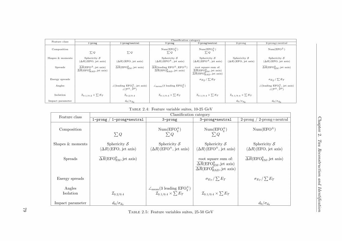
Ch
apter
2.T
au
Reco
nstru
ction
an
dId
entifi
catio
n
Feature classClassification category
1-prong 1-prong+neutral 3-prong 3-prong+neutral 2-prong 2-prong+neutral
Composition Num(EFO±q ) Num(EFO±
q ) Num(EFO±)∑Q
∑Q
∑Q
∑Q
Shapes & moments Sphericity S Sphericity S Sphericity S Sphericity S Sphericity S〈∆R〉(EFO, jet axis) 〈∆R〉(EFO, jet axis) 〈∆R〉(EFO±, jet axis) 〈∆R〉(EFO±, jet axis) 〈∆R〉(EFO, jet axis) 〈∆R〉(EFO, jet axis)
Spreads ∆R(EFO±, jet axis) ∆R(EFO0EM, jet axis) ∆R(leading EFO±,EFO±) root square sum of: ∆R(EFO0
EM, jet axis)
∆R(EFO0HAD, jet axis) ∆R(EFO0
HAD, jet axis) ∆R(EFO0EM, jet axis)
∆R(EFO0HAD, jet axis)
Energy spreads σET/∑ET σET
/∑ET
Angles ∠(leading EFO±q , jet axis) ∠mean(3 leading EFO±
q ) ∠(leading EFO±q , jet axis)
∠(P±,P0) ∠(P±,P0)
Isolation I0.1/0.2 ×∑ET I0.2/0.4 I0.1/0.4 ×
∑ET I0.1/0.4 ×
∑ET I0.1/0.4 ×
∑ET
Impact parameter d0/σd0 d0/σd0 d0/σd0
Table 2.4: Feature variable suites, 10-25 GeV
Feature classClassification category
1-prong / 1-prong+neutral 3-prong 3-prong+neutral 2-prong / 2-prong+neutral
Composition Num(EFO±q ) Num(EFO±q ) Num(EFO±)∑Q
∑Q
∑Q
Shapes & moments Sphericity S Sphericity S Sphericity S Sphericity S〈∆R〉(EFO, jet axis) 〈∆R〉(EFO±, jet axis) 〈∆R〉(EFO±, jet axis) 〈∆R〉(EFO, jet axis)
Spreads ∆R(EFO0EM, jet axis) root square sum of: ∆R(EFO0
EM, jet axis)∆R(EFO0
EM, jet axis)∆R(EFO0
HAD, jet axis)
Energy spreads σET/∑ET σET
/∑ET
Angles ∠mean(3 leading EFO±q )Isolation I0.2/0.4 I0.1/0.4 ×
∑ET I0.1/0.4 ×
∑ET
Impact parameter d0/σd0 d0/σd0
Table 2.5: Feature variables suites, 25-50 GeV
79
Chapter 2. Tau Reconstruction and Identification
as electromagnetic 19. Whenever resolved and properly tagged, EM neutral EFOs are
expected to be located close to the jet axis in τ -induced seeds, whereas a larger spread
can be expected in jet-induced seeds.
Candidate feature selections chosen for this category are again listed in Tables 2.4 and
2.5. The presence of additional neutrals in both signal and background provides more
handles for separation, e.g. through the use of angular relations.
The discriminating power of these features with respect to jet-induced seeds are depicted
in Figures 2.26 and 2.27, indicating a clear improvement when compared to the 1-prong
category.
2.4.5.3 Category: 3-prong
The 3-prong category has the second highest ”purity” of all the categories, with roughly
70% of all τ -induced seeds decending from the target process τ± → π±π∓π±. The large
majority (∼ 90%) of these τ -induced seeds will contain precisely three charged qualified
EFOs. These EFO±q provide a distinct handle on the separation of τ -induced seeds from
jet-induced seeds in this category.
The feature suites considered at low and intermediate transverse momenta are listed
in Tables 2.4 and 2.5, and a comparison of these features in signal and background is
provided in Figures 2.28 and 2.29.
2.4.5.4 Category: 3-prong+neutral
Unlike the 3-prong category, the 3-prong+neutral category contains a significant ad-
mixture of different true τ -decays. While 60% of τ -induced seeds in this category de-
scend from 3-prong decays, almost 35% stem from falsely classified π± + nπ0 decays.
This ”contamination” from 1-prong decays dilutes some of the discriminating power seen
in the variables involving the leading charged EFOs seen in the 3-prong category. The
challenge is exacerbated by the large background in this channel, the largest of all the
X-prong(+neutral) categories.
The feature suites considered at low and intermediate transverse momenta are listed
in Tables 2.4 and 2.5, and a comparison of these features in signal and background is
provided in Figures 2.30 and 2.31.
2.4.5.5 Category: 2-prong
The 2-prong category contains the largest admixture of different τ -induced seeds, and
consequently presents itself as the most challenging category. With roughly one half
19It should be noted, that while it is possible that the decay π0 → γγ may yield two resolved γ-clusters,studies have shown this to be a comparatively rare occurance (∼ 5%) in ATLAS [71].
80
Chapter 2. Tau Reconstruction and Identification
stemming from 1-prong decay modes and the other from 3-prong decay modes, it be-
comes increasingly more difficult to identify features that capture the unique properties
of each decay topology. This problem is exacerbated by the ∼ 2 : 3 ratio of 1-prong
induced seeds from π± to 1-prong induced seeds from π±+ nπ0. Hence a small variable
suite is chosen at low transverse momenta, focusing largely on the global properties of
classified seeds. These are listed in Table 2.4 and a comparison of the corresponding dis-
tributions in signal and background are shown in Figure 2.32. At intermediate transverse
momenta, this category is trained together with the 2-prong+neutral category.
2.4.5.6 Category: 2-prong+neutral
While the 2-prong+neutral category also contains a comparatively large admixture of
τ -induced seeds with different decay mode origin, it is dominated by falsely classified
seeds stemming from π± + nπ0 decays (∼ 67%), the remainder consisting of a roughly
equal admixture of 3π± and 3π±+nπ0. This asymmetry in the admixture makes it easier
to identify defining features with separation power. The high fraction of π±+nπ0 decays
found in this category, motivates feature suites resembling those of 1-prong+neutral.
These are listed in Tables 2.4 and 2.5 and the corresponding feature distributions shown
in Figures 2.33 and 2.34.
2.4.6 Likelihood discriminants and performance evaluation
As was already alluded to in Section 2.4.5, the discriminating power of the variables
suites defined for each reconstruction category can typically be enhanced if the variables
are combined into a single multivariate discriminant. While a wide range of methods of
varying complexity (and transparency) are available, only a simple projective likelihood
approach will be considered herein.
For a given reconstruction category, the projective likelihood is defined in terms of the
likelihood ratio, which for each PanTau seed may be expressed as:
LR =Lτ
Lτ + Ljet. (2.22)
The likelihood functions Lτ/jet are products of the individual probability density functions
Pτ/jet of the input variables pertaining to the category under consideration:
Lτ/jet =
Nfeatures∏i=1
P iτ/jet(xi) (2.23)
The probability density functions Pτ/jet are in turn derived from polynomial splines
fitted to the input variable distributions listed in the previous section and normalized
such that:
81

Chapter 2. Tau Reconstruction and Identification
∫ +∞
−∞Pτ/jet(xi)dxi = 1 (2.24)
As such, the likelihood ratio provides a comparatively simple way to combine the in-
formation in the various input variables into a single measure of the probability that a
given PanTau seed might have originated from a true τ -decay (LR → 1) or from the
hadronization of quarks and gluons (LR → 0).
While the projective likelihood as defined above will generally deliver optimal results
with uncorrelated input variables, its performance is likely to degrade in the presence
of correlations. The inclusion of strongly correlated feature variables has been avoided
whenever possible in the feature selections presented in Section 2.4.5, however non-trivial
and non-linear correlations do persist between input variables within in each category.
In some cases, these correlations are observed to give rise to double peak structures (at
LR ∼ 0 and LR ∼ 1) in the projective likelihoods for τ -induced and/or jet-induced seeds
[72].
Correlations between input variables in a given reconstruction category can scarcely be
avoided and some performance degradation is therefore expected to follow. However,
more than optimizing the separation of τ -induced seeds from falsely classified jet-induced
seeds, the purpose of the following study is to identify and highlight the merits and
shortcomings of the PanTau approach to τ -reconstruction and identification compared
to canonical approaches to τ -reconstruction in ATLAS. To this end, the projective like-
lihood presents itself as a simple and transparent method with respect to which more
complicated and refined methods that are less sensitive to correlations may later be
compared.
The likelihood distributions resulting from each of the variable suites presented in Section
2.4.5 are shown in Figures 2.16 and 2.17. Despite the strong resemblance between τ -
induced and jet-induced seeds classified in the same category, a decent discrimination is
achieved in most reconstructed categories, both at low and intermediate momenta. As
expected, the separation power offered by the likelihood in the categories 1-prong and
2-prong is comparatively poor, a reflection of the difficulty of identifying sufficiently
robust discriminating features in these categories.
In order to assess the utility of PanTau, it is helpful and instructive to compare its
performance with standard τ -reconstruction tools in ATLAS. Such a comparison should
ideally be insensitive to the details of any underlying technical differences between the
algorithms or their reconstructed input. To this end, the performance comparison will
herein be expressed in terms of the signal identification efficiency εS :
εS =Number of tagged τ -candidates ∧ (match to τMC)
Number of τMC(2.25)
and the fake rate:
82

Chapter 2. Tau Reconstruction and Identification
(a) 1-prong (10-25 GeV) (b) 1-prong (25-50 GeV)
(c) 1-prong+neutral (10-25 GeV) (d) 1-prong+neutral (25-50 GeV)
(e) 3-prong (10-25 GeV) (f) 3-prong (25-50 GeV)
(g) 3-prong+neutral (10-25 GeV) (h) 3-prong+neutral (25-50 GeV)
Figure 2.16: Likelihood distributions: 1-prong and 3-prong categories (all distribu-tions are transformed by an inverse sigmoid).
83

Chapter 2. Tau Reconstruction and Identification
(a) 2-prong (10-25 GeV) (b) 2-prong (25-50 GeV)
(c) 2-prong+neutral (10-25 GeV) (d) 2-prong+neutral (25-50 GeV)
Figure 2.17: Likelihood distributions: 2-prong categories (all distributions are trans-formed by an inverse sigmoid).
εFR =Number of tagged τ -candidates ∧ ¬(match to τMC)
Number of events(2.26)
The latter quantity may be more conveniently expressed in terms of the ”rejection”:
R =1− εFRεFR
(2.27)
In either case, a tagged τ -candidate is understood as a reconstructed and identified
candidate produced by the algorithm under consideration. A track-based matching
scheme has been employed to relate reconstructed τ -candidates with Monte Carlo τ
(τMC) by way of an association between reconstructed and true tracks [73].
The reader is advised that the above definition of the rejection differs from the standard
definitions of background rejection employed by the ATLAS Tau Working Group [55, 74].
The latter will typically define the rejection in terms of the background efficiency:
εB =Number of tagged τ -candidates ∧ ¬(match to τMC)
Number of MC jets
84

Chapter 2. Tau Reconstruction and Identification
While this measure has the benefit of normalizing to a quantity that is independent of
the details of the reconstruction, it fails to account for any effects or objects that may
not find an appropriate Monte Carlo jet match, yet still generate a fake seed for the
reconstruction algorithm. Alternatively, one may choose to replace the quantity in the
denominator with the number of reconstructed τ -candidates. Such a measure would take
due account of fake seeds without an appropriate Monte Carlo jet match, but equally be
sensitive to differences in the way in which the algorithms define their τ -candidates (i.e.
it is possible that a given seed for algorithm A would never qualify for algorithm B, and
vice versa). In order to provide a measure of comparison where such subtle effects are
minimized, the rejection is herein defined in terms of the fake rate as given by equation
2.26.
Performance comparisons in the εS − R plane for PanTau and the standard ATLAS
τ -reconstruction package tauRec are provided below. It is notable that the compari-
son is performed against tauRec candidates that are either calorimeter seeded or both
calorimeter and track seeded, i.e. two dedicated τ -reconstruction packages, rather than
one. In all cases, Z → ττ and W → τντ has been used as sources of τ -induced seeds,
whereas a cross-section weighted mixture of QCD dijets covering the hard scattering
range 8-140 GeV has been used as a source of jet-induced seeds. Any jet-induced seeds
from the Z and W samples have been omitted, as have any τ -induced seeds originating
from non-isolated τ -leptons in QCD. All performance comparisons are performed within
|ηseed| <2.0 to stay well within the sensitivity range of the inner detector.
Global performance
The overall performance of PanTau with respect to true 1-prong and 3-prong decays is
compared to that of tauRec in Figures 2.18 and 2.19, respectively. The measure includes
PanTau candidates from all reconstructed categories, save Other. For just comparison,
tauRec candidates are required to have between 1 and 4 associated tracks.
PanTau is seen to underperform with respect to tauRec, whereby the relative differ-
ences in performance are more accentuated at low transverse momenta. At intermediate
momenta, the performances are seen to converge at high efficiency (εS >60%).
As was discussed above, the quality of the PanTau likelihood discriminants varies across
the different reconstruction categories depending on the relative composition of τ -induced
seeds in each category. Moreover, some categories are found to be significantly more sen-
sitive to background contamination than others. Poor performance in one reconstruction
category may therefore diminish the global performance considerably. It is therefore in-
structive to compare the reconstruction and identification performance of specific decay
modes with due regard to the migration matrix shown in Figure 2.14.
1-prong performance
As indicated in Figure 2.14, the categories 1-prong+neutral and 2-prong+neutral
both enjoy a high fraction of τ -induced seeds from τvis → π± + nπ0 decays, with small
or moderate admixtures of seeds from other decay modes. The high ”purity” enjoyed
85

Chapter 2. Tau Reconstruction and Identification
(a) 10-25 GeV
(b) 25-50 GeV
Figure 2.18: Global performance w.r.t. true 1-prong decays (excl. Kaons) for can-didates with transverse momenta between (a) 10-25 GeV and (b) 25-50 GeV. PanTaucandidates from all reconstructed categories except from Other are considered. tauRec
candidates are accordingly required to have between 1 and 4 associated tracks.
86
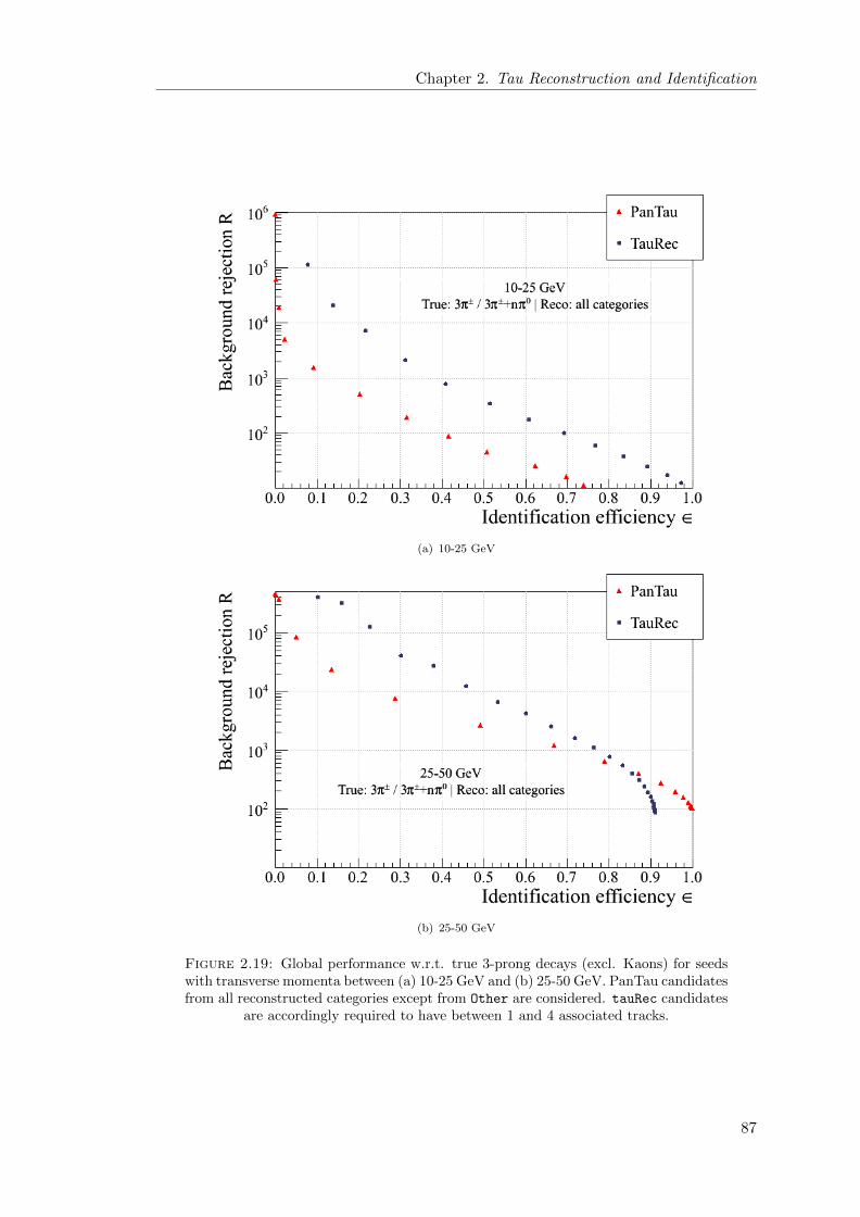
Chapter 2. Tau Reconstruction and Identification
(a) 10-25 GeV
(b) 25-50 GeV
Figure 2.19: Global performance w.r.t. true 3-prong decays (excl. Kaons) for seedswith transverse momenta between (a) 10-25 GeV and (b) 25-50 GeV. PanTau candidatesfrom all reconstructed categories except from Other are considered. tauRec candidates
are accordingly required to have between 1 and 4 associated tracks.
87

Chapter 2. Tau Reconstruction and Identification
in these categories better facilitates the construction of variables sensitive to the char-
acteristic signatures of such decays, and consequently an improvement with respect to
the global 1-prong performance might be expected in these channels.
Figure 2.20 compares the performance with respect to true τvis → π± + nπ0 decays
using only PanTau candidates from the categories 1-prong, 1-prong+neutral and
2-prong+neutral and indicates that a more commensurate performance can be achieved
when using 1-prong candidates from either of these categories. (The latter category is
included in order to extend the efficiency beyond the ∼ 70% of true τvis → π± + nπ0
decays classified as 1-prong or 1-prong+neutral(see Figure 2.12)).
3-prong performance
A similar tendency is observed in the 3-prong sector, albeit only at intermediate trans-
verse momenta. Here the 3-prong category is the only category dominated by τvis →π±π∓π± decays, although 2-prong also contains a significant portion of τvis → π±π∓π±
induced seeds. The performance with respect to true τvis → π±π∓π± decays in these
categories is shown in Figure 2.21 which indicates a competitive performance at inter-
mediate efficiencies (εS > 50%). At lower transverse momenta, the PanTau performance
deteriorates as a result of the diminished likelihood separation in the 3-prong category
in this kinematic region.
While the above results indicate that further improvements are required before Pan-
Tau can be considered a mature and competitive τ -reconstruction tool, they also clearly
vindicate the merits of the driving principles in PanTau. The performance convergence
observed in the most performant and well-behaved reconstruction modi, successfully
demonstrates that it is possible to apply the principles of particle flow to lepton recon-
struction in ATLAS.
2.4.6.1 Transverse energy resolutions
It is instructive to compare the transverse energy resolutions of τ -candidates in PanTau
and tauRec. The precise resolution of the final PanTau τ -objects made available for
analysis are likely to depend on their precise definition20. At the time of writing these
considerations are still ongoing, and the comparison herein will therefore include all
constituent EFOs of a PanTau seed.
Figures 2.22 and 2.23 respectively compare the transverse energy resolutions of 1-prong
induced candidates reconstructed as either 1-prong or 1-prong+neutral and that of 3-
prong induced candidates reconstructed as either 3-prong or 3-prong+neutral. Distri-
butions are shown before and after the application of a moderate identification selection
corresponding to εS ∼ 40%.
It is evident that PanTau tends to overestimate the ET of both 1-prong and 3-prong
induced candidates by roughly 6-8% at low transverse momenta and by 9-10% at more
20i.e should the final category 3-prong candidate include all EFOs found in its corresponding seed, orjust the three leading EFO±q ?
88

Chapter 2. Tau Reconstruction and Identification
(a) 10-25 GeV
(b) 25-50 GeV
Figure 2.20: Performance comparison w.r.t. τ±vis → π± + nπ0 decays for seeds withtransverse momenta between (a) 10-25 GeV and (b) 25-50 GeV. Only candidates fromthe PanTau categories 1-prong, 1-prong+neutral and 2-prong+neutral are consid-
ered. tauRec candidates are required to have between 1 and 2 tracks.
89

Chapter 2. Tau Reconstruction and Identification
(a) 10-25 GeV
(b) 25-50 GeV
Figure 2.21: Performance comparison w.r.t. τ±vis → 3π± decays for seeds with trans-verse momenta between (a) 10-25 GeV and (b) 25-50 GeV. Only candidates from thePanTau categories 3-prong and 2-prong are considered. tauRec candidates are re-
quired to have between 2 and 4 tracks.
90

Chapter 2. Tau Reconstruction and Identification
intermediate transverse momenta. By comparison, tauRec typically underestimates the
ET by circa 0.1-1% in the 1-prong sector and 2-5% in the 3-prong sector at all transverse
momenta. The tendency for eflowRec to overestimate the energy scale of single 1-prong
τ -leptons was briefly mentioned in Section 2.3.2.4 and is reported in [62], however it is
notable that this effect appears to be more pronounced in PanTau, especially at inter-
mediate transverse momenta21. In most cases, the identification is seen to be insensitive
to the overestimation, save in the 3-prong sector at low transverse momenta where it is
seen to favour candidates with an overesimated ET .
The PanTau ET -resolution distributions are moreover seen to be positively skewed (with
broader right-sided tails). This (non-gaussian) asymmetry makes the determination of
resolutions by way of gaussian fits challenging. Herein, the resolutions will therefore
rather be compared in terms of truncated standard deviations. Table 2.6 compares the
standard deviation of the resolution distributions for PanTau and tauRec truncated at
1.0σ and 1.5σ to either side of their respective means. The table also lists the associated
mean (x), skewness22 (Γ) and kurtosis23 (K). According to Table 2.6, PanTau typically
achieves a better resolution at low transverse momenta, but deteriorates slightly with
increasing τ -lepton energy. As expected, this effect is more pronounced in the 3-prong
sector.
Even if the skews are reduced by > 50% after truncation, they remain large when
compared to tauRec. The larger kurtoses observed in PanTau indicate that while the
resolutions are more strongly peaked than in tauRec with the majority of candidates
reconstructed with small deviations from the mean, broader and longer tails persist
where deviations are considerable.
2.4.6.2 Resolving decay resonances
As was discussed early in this Chapter (Sections 2.1.2 and 2.1.3 ), analyses involving τ -
leptons will sometimes want to extract polarization information from the reconstructed
τ -object. The quality of any polarization sensitive measurement will typically depend
on how well the τ -reconstruction tool is able to determine the original decay mode of the
reconstructed τ -object [75]. Because the base unit of PanTau is a reconstructed ”pion”-
object, the algorithm is expected to retain a comparatively high degree of sensitivity to
the details of the τ -decay. It is therefore instructive to consider how well the mass peaks
corresponding to mesonic resonances by which the large majority of τ -leptons decay can
be reconstructed.
21It should be noted that the simulated data samples used herein employ an older version of theeflowRec software than that used to produce the results reported in Section 2.3.2.4. Several bug-fixesin the underlying eflowRec software have since been introduced which may impact the results presentedherein. At the time of writing, these new fixes have not been tested in the context of PanTau. Differencesin the respective seed building procedures may also account for the higher overestimation observed inPanTau.
22The skewness provides a measure for the asymmetry of the distribution, where a positive skew(Γ > 0) corresponds to a left-skew and a negative skew (Γ < 0) corresponds to a right-skew.
23The kurtosis indicates how peaked the distribution is with respect to a gaussian distribution. Ahigher kurtosis implies that deviations from the mean are infrequent but large, rather than comparativelyfrequent, but small.
91

Chapter 2. Tau Reconstruction and Identification
(a) 1-prong: 10-25 GeV, |η| < 2.0 (b) 1-prong: 25-50 GeV, |η| < 2.0
Figure 2.22: Transverse energy resolution of candidates matched to true 1-prongτ -leptons from Z → ττ . PanTau candidates are drawn from the 1-prong and1-prong+neutral categories. tauRec candidates are required to have 1 associatedtrack. The identification selection applied to PanTau candidates correspond to εS ∼
40%.
(a) 3-prong: 10-25 GeV,|η| < 2.0 (b) 3-prong: 25-50 GeV,|η| < 2.0
Figure 2.23: Transverse energy resolution of candidates matched to true 3-prongτ -leptons from Z → ττ . PanTau candidates are drawn from the 3-prong and3-prong+neutral categories. tauRec candidates are required to have 3-4 associ-ated tracks.The identification selection applied to PanTau candidates correspond to
εS ∼ 40%.
92

Chapter 2. Tau Reconstruction and Identification
(a) 1-prong, 10-25 GeV
Global (no truncation) x± 1.0σx x± 1.5σxPanTau TauRec PanTau TauRec PanTau TauRec
x 1.0785±0.0006 0.9943±0.0005 1.0636±0.0003 0.9926±0.0003 1.0643±0.0004 0.9896±0.0004σ 0.1596±0.0004 0.1504±0.0003 0.0780±0.0002 0.0779±0.0002 0.1036±0.0003 0.1046±0.0002Γ 0.938±0.009 0.554±0.008 0.31±0.01 0.004±0.009 0.2718±0.009 0.003±0.008K 2.90±0.02 2.32±0.02 -0.72±0.02 -0.93±0.02 -0.39±0.02 -0.69±0.02
(b) 1-prong, 25-50 GeV
Global (no truncation) x± 1.0σx x± 1.5σxPanTau TauRec PanTau TauRec PanTau TauRec
x 1.1095±0.0006 1.0100±0.0005 1.0890±0.0003 1.0027±0.0003 1.0908±0.0004 0.9989±0.0003σ 0.1447±0.0004 0.1275±0.0004 0.0735±0.0002 0.0626±0.0002 0.0943±0.0003 0.0816±0.0002Γ 1.49±0.01 1.67±0.01 0.38±0.01 0.11±0.01 0.38±0.01 0.10±0.01K 4.94±0.02 8.18±0.02 -0.77±0.02 -0.80±0.02 -0.44±0.02 -0.45±0.02
(c) 3-prong, 10-25 GeV
Global (no truncation) x± 1.0σx x± 1.5σxPanTau TauRec PanTau TauRec PanTau TauRec
x 1.095±0.001 0.958±0.001 1.0730±0.0006 0.9535±0.0003 1.0766±0.0008 0.9505±0.0008σ 0.1528±0.0008 0.1570±0.0007 0.0732±0.0004 0.0830±0.0004 0.0975±0.0005 0.1124±0.0005Γ 1.14±0.02 0.59±0.02 0.48±0.02 0.07±0.02 0.44±0.02 0.07±0.02K 3.19±0.04 1.77±0.03 -0.57±0.04 -0.99±0.04 -0.22±0.04 -0.78±0.03
(d) 3-prong, 25-50 GeV
Global (no truncation) x± 1.0σx x± 1.5σxPanTau TauRec PanTau TauRec PanTau TauRec
x 1.120±0.0008 0.9926±0.0009 1.092±0.0005 0.9825±0.0005 1.0960±0.0006 0.9787±0.0006σ 1.149±0.0006 0.1359±0.0006 0.0755±0.0003 0.0689±0.0004 0.0960±0.0004 0.0907±0.0004Γ 1.56±0.01 1.59±0.02 0.52±0.01 0.15±0.02 0.53±0.01 0.14±0.02K 4.27±0.03 6.75±0.03 -0.64±0.03 -0.85±0.04 -0.33±0.03 -0.54±0.03
Table 2.6: Global and truncated mean values (x), standard deviations (σ), skewness(Γ) and kurtosis (K) derived from ET -resolution distributions for PanTau and tauRec.
Truncations are performed at 1.0σ and 1.5σ to either side of the global mean.
Figure 2.24 shows an attempt to reconstruct the mass peaks corresponding to the two
multi-pion 1-prong decays:
τ±vis → ρ±(770 MeV)→ π±π0
and
τ±vis → a±1 (1230 MeV)→ π±π0π0
using τ -induced candidates from the 1-prong+neutral category. Invariant mass distri-
butions obtained using all EFOs in the seed-jet are contrasted with the corresponding
distributions using only significant EFOs, where the latter quantity comprises all EFO±
and all EFO0EM in the seed.
The effect of additional non-tau related EFOs in the seed jet is to wash out the mass
peaks. These mass peaks can be recovered if the appropriate particle objects are cor-
rectly identified, a task which becomes increasingly more difficult as the transverse
93

Chapter 2. Tau Reconstruction and Identification
(a) PanTau: 10-25 GeV (b) PanTau: 25-50 GeV
(c) TauRec
Figure 2.24: (a)-(b) Invariant mass distributions derived from τ -induced seeds clas-sified in the category 1-prong+neutral. The invariant mass of all constituents iscontrasted with the invariant mass of EFO± and EFO0
EM. Mass peaks are observablebut are seen to wash out as the decay system becomes more collimated. The invariantmass distributions of the EFO±q -system in seeds from the category 3-prong are shownfor comparison. (c) Invariant mass using dedicated π0-reconstruction in tauRec [55].
momenta increases and the boost renders the decay system more collimated. Despite
the comparatively fat tails observed in the ρ-distributions in either regime (an effect
which is believed to be related to the overestimation of energy in τ±vis → ρ± → π±π0
decays in eflowRec), the invariant mass distributions of PanTau are still seen to com-
pare favourably to those obtained with dedicted π0-subclustering routines in tauRec.
The invariant mass of the EFO±q -sytem in 3-prong reconstructed seeds originating from
τ±vis → a±1 → π±π∓π± decays, is shown for comparison. It is evident that an accurate
reconstruction and identification of π0 inside the seed jet is an important prerequisite
for a precise decay mode estimation.
94

Chapter 2. Tau Reconstruction and Identification
2.5 Summary
In the hadronic environment of the LHC, accurate and efficient τ -reconstruction tools
are imperative to enable a full exploitation of the physics potential of the LHC. The
availability of several unique and distinct approaches to the reconstruction of τ -leptons
is therefore an important asset to the experiment, which when used in combination may
facilitate an improved interpretation of the recorded data.
With the development of ever more granular calorimeters capable of separating close
lying showers, the concept of ”particle flow” has emerged as a promising method of
combining and condensing information from all subdetectors into an event description
in which the unit objects may (ideally) be identified with the stable particles of the
event. The prerequisites for successful particle flow calorimetry comprise both the hard-
ware ability to resolve energy deposits from different particles and the software ability to
reconstruct and identify deposits from individual particles. To ensure that both require-
ments are satisfied, both hardware and software for next generation collider experiments
are typically developed in parallel, both driven by the concepts of particle flow [76]. As
the ATLAS detector was conceived and constructed in a different manner, it is therefore
not a priori clear to what extent a full-fledged particle level event description can be
achieved.
The studies herein sought to explore the potential for applying the ideas of particle flow
calorimetry in the context of τ -reconstruction and identification in ATLAS. To this end,
a novel reconstruction algorithm named PanTau has been developed in a collaborative
effort with S. Fleischmann.
It was shown that it is possible to disentangle the constituents of the τ -decay in the
ATLAS calorimeters, and that improved energy resolutions can be obtained if the calori-
metric energy deposits of charged particles is duly replaced by the corresponding mo-
mentum measurement from the tracker. In ATLAS, the latter operation is performed on
all calorimeter clusters with an associated track using a generic energy flow technique
known as eflowRec, the output of which forms the raw input to PanTau.
Rather than viewing the τ -lepton as a narrow jet, PanTau seeks to recognize decay
topologies that are physically consistent with a hadronically decaying τ -lepton using
information from the resolved objects in the decay wake. This approach allows for an
early classification of τ -candidates according to their most probable decay mode and an
equally early rejection of candidates found inconsistent with the decay of a τ -lepton.
The classification scheme naturally invites usage of decay-mode specific discriminants
against fake candidates from QCD, and it was demonstrated how discriminants with
significant separation power can be built from the constituent objects alone, without
directly drawing on information from the calorimeters or the tracker.
Though the overall identification performance was found lacking when compared to
canonical τ -reconstruction tools in ATLAS, it was demonstrated that a comparable per-
formance can be achieved in the most performant reconstruction modi of PanTau. While
95

Chapter 2. Tau Reconstruction and Identification
further improvements are required before the algorithm is fully on par with existing τ -
reconstruction tools in ATLAS, these results serve as a vindication of the feasibility
of the method and the merits of the underlying ideas. It was also shown that Pan-
Tau is sensitive to the decay modes of the τ -lepton and generally provides an improved
transverse energy resolution. As all steps in the algorithm, including the building of
discriminating features, rely squarely on the resolved objects of the decay, PanTau is
distinguished insofar as it maintains a clear and natural separation between detector
effects and the physics of the τ -lepton decay.
96

Chapter 2. Tau Reconstruction and Identification
(a)∑Q (b) (*) ∆R(EFO±, jet axis)
(c) ∆R(EFO0HAD, jet axis) (d) (*) I0.1/0.2 ×
∑ET
(e) (*) Sphericity S (f) (*) 〈∆R〉(EFO, jet axis)
Figure 2.25: Feature distributions: 1-prong, 10 GeV < pseedT < 25 GeV, (|ηseed| <2.0). Distributions marked with an (*) are strongly peaked and have been transformed
with an inverse sigmoid function.
97

Chapter 2. Tau Reconstruction and Identification
(a)∑Q (b) ∆R(EFO0
EM, jet axis)
(c) 〈∆R〉(EFO, jet axis) (d) (*) I0.2/0.4
(e) ∠(leading EFO±q , jet axis) (f) ∠(P±,P0)
(g) d0/σd0
Figure 2.26: Feature distributions: 1-prong+neutral, 10 GeV < pseedT < 25 GeV,(|ηseed| < 2.0). Distributions marked with an (*) have been transformed with an inverse
sigmoid function.
98

Chapter 2. Tau Reconstruction and Identification
(a)∑Q (b) ∆R(EFO0
EM, jet axis)
(c) 〈∆R〉(EFO, jet axis) (d) (*) I0.2/0.4
(e) (*) Sphericity S (f) d0/σd0
Figure 2.27: Feature distributions: 1-prong / 1-prong+neutral, 25 GeV < pseedT <50 GeV, (|ηseed| < 2.0). Distributions marked with an (*) have been transformed with
an inverse sigmoid function.
99
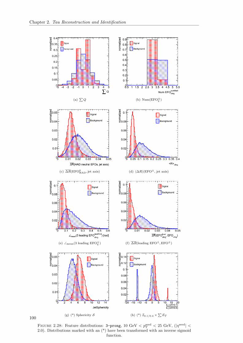
Chapter 2. Tau Reconstruction and Identification
(a)∑Q (b) Num(EFO±q )
(c) ∆R(EFO0HAD, jet axis) (d) 〈∆R〉(EFO±, jet axis)
(e) ∠mean(3 leading EFO±q ) (f) ∆R(leading EFO±,EFO±)
(g) (*) Sphericity S (h) (*) I0.1/0.4 ×∑ET
Figure 2.28: Feature distributions: 3-prong, 10 GeV < pseedT < 25 GeV, (|ηseed| <2.0). Distributions marked with an (*) have been transformed with an inverse sigmoid
function.
100

Chapter 2. Tau Reconstruction and Identification
(a)∑Q (b) Num(EFO±q )
(c) 〈∆R〉(EFO±, jet axis) (d) ∠mean(3 leading EFO±q )
(e) (*) Sphericity S (f) (*) I0.1/0.4 ×∑ET
Figure 2.29: Feature distributions: 3-prong, 25 GeV < pseedT < 50 GeV, (|ηseed| <2.0). Distributions marked with an (*) have been transformed with an inverse sigmoid
function.
101
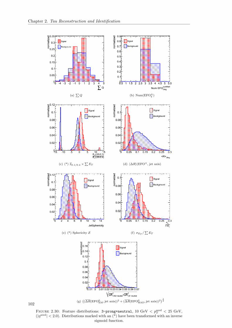
Chapter 2. Tau Reconstruction and Identification
(a)∑Q (b) Num(EFO±q )
(c) (*) I0.1/0.4 ×∑ET (d) 〈∆R〉(EFO±, jet axis)
(e) (*) Sphericity S (f) σET/∑ET
(g)((∆R(EFO0
EM, jet axis))2 + (∆R(EFO0HAD, jet axis))2
) 12
Figure 2.30: Feature distributions: 3-prong+neutral, 10 GeV < pseedT < 25 GeV,(|ηseed| < 2.0). Distributions marked with an (*) have been transformed with an inverse
sigmoid function.
102

Chapter 2. Tau Reconstruction and Identification
(a)∑Q (b) Num(EFO±q )
(c) (*) I0.1/0.4 ×∑ET (d) 〈∆R〉(EFO±, jet axis)
(e) (*) Sphericity S (f) σET/∑ET
(g)((∆R(EFO0
EM, jet axis))2 + (∆R(EFO0HAD, jet axis))2
) 12
Figure 2.31: Feature distributions: 3-prong+neutral, 25 GeV < pseedT < 50 GeV,(|ηseed| < 2.0). Distributions marked with an (*) have been transformed with an inverse
sigmoid function.
103

Chapter 2. Tau Reconstruction and Identification
(a) 〈∆R〉(EFO, jet axis) (b) (*) I0.1/0.4 ×∑ET
(c) d0/σd0 (d) (*) Sphericity S
Figure 2.32: Feature distributions: 2-prong, 10 GeV < pseedT < 25 GeV, (|ηseed| <2.0). Distributions marked with an (*) have been transformed with an inverse sigmoid
function.
104
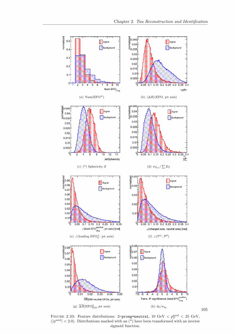
Chapter 2. Tau Reconstruction and Identification
(a) Num(EFO±) (b) 〈∆R〉(EFO, jet axis)
(c) (*) Sphericity S (d) σET/∑ET
(e) ∠(leading EFO±q , jet axis) (f) ∠(P±,P0)
(g) ∆R(EFO0EM, jet axis) (h) d0/σd0
Figure 2.33: Feature distributions: 2-prong+neutral, 10 GeV < pseedT < 25 GeV,(|ηseed| < 2.0). Distributions marked with an (*) have been transformed with an inverse
sigmoid function.
105
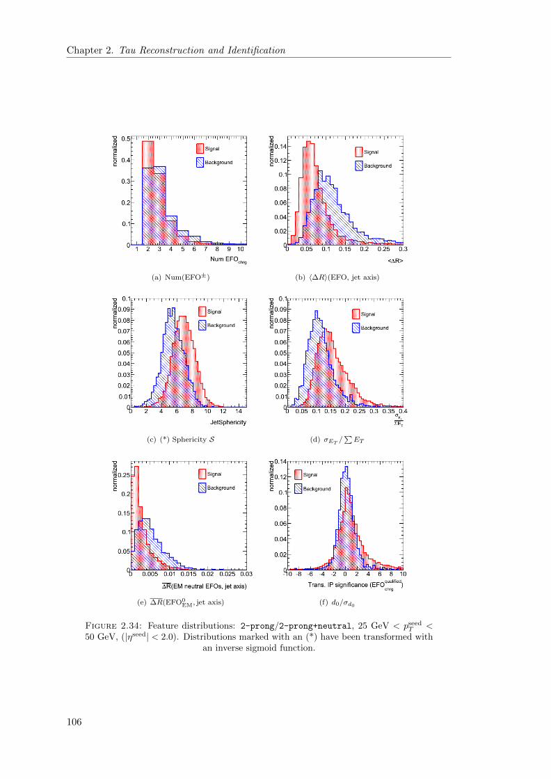
Chapter 2. Tau Reconstruction and Identification
(a) Num(EFO±) (b) 〈∆R〉(EFO, jet axis)
(c) (*) Sphericity S (d) σET/∑ET
(e) ∆R(EFO0EM, jet axis) (f) d0/σd0
Figure 2.34: Feature distributions: 2-prong/2-prong+neutral, 25 GeV < pseedT <50 GeV, (|ηseed| < 2.0). Distributions marked with an (*) have been transformed with
an inverse sigmoid function.
106
Chapter 3
A method to improve Monte
Carlo statistics of QCD induced
instrumental /ET
While most electromagnetically and hadronically interacting particles are absorbed in
the calorimeters and the momenta of charged MIPs such as µ± are measured in the
muon spectrometer, weakly interacting (neutral) particles scarcely react with the detector
material and consequently escape the experimental volume undetected.
The only method of identifying such particles is by way of inference: if all particles in the
event were accounted for, the sum energy-momentum measured in the detector should
ideally equal the√s of the colliding beams. Any discrepancy, often termed /E, may then
be attributed to particles escaping undetected.
At hadron colliders such as the LHC however, this method cannot be straightforwardly
applied to infer the presence of weakly interacting particles. As discussed in Section
1.3.1, the initial momentum fraction carried by the colliding parton constituents is a
priori unknown and hadronic debris scattered at small angles down the beam pipe,
render the longitudinal momentum component unmeasurable. However, insofar as the
transverse momentum component of the incoming partons is negligible (pz pT ), a
momentum balance may still be inferred in the transverse (x,y) plane:
∑ET + /ET = 0 (3.1)
whereupon the missing transverse energy ( /ET ) can be defined as:
/ET = −
√√√√(∑n
Ex
)2
+
(∑n
Ey
)2
. (3.2)
107

Chapter 3. Improving MC statistics of QCD induced instrumental /ET
The sums in Equation 3.2 may run over calorimeter cells, energy flow objects, recon-
structed particle object or combinations thereof.
The ν is the most frequent neutral weakly interacting particle to accompany both ex-
pected and anticipated processes at the LHC. Because ν emerge not only from τ -lepton
decays as discussed in Chapter 2, but also from leptonic decays of W and Z bosons and
from semi-leptonic decays heavy flavour quarks, they constitute a frequent source of /ET .
The ability to accurately quantify the event /ET induced from escaping ν is therefore of
importance to both W and top mass measurements [32], as well as in the search and
measurement of new physics processes such as H → W±W∓ or H → τ±τ∓. Moreover,
underpinned by astrophysical data suggesting an abundance of dark matter in the Uni-
verse, several models of physics beyond the Standard Model predict heavy stable neutral
weakly interacting particles. In particular, the collider phenomenology of all R-parity
conserving SUSY models involves a stable and neutral lightest supersymmetric particle
(LSP) which escapes direct experimental detection and typically renders the event sep-
arable from background by way of a large momentum imbalance. Signatures involving
large /ET beyond Standard Model predictions are thus strongly indicative of new physics
and it is therefore critically important to correctly quantify the event /ET .
3.1 Calculating /ET in ATLAS
ATLAS employs various methods to compute the event /ET , including the so-called
cell-based method, the object based method and the energy flow based method [66]. As
the standard method in ATLAS, the cell-based approach has been used in all studies
presented herein. Therefore, the following provides a cursory description of the cell-based
technique only.
The cell-based method computes the event /ET as the vectorial sum of transverse energy
deposited in the calorimeters and the momenta measured in the muon spectrometer,
applying due corrections for potential energy losses in the cryostat surrounding the
ECAL:
/Ex,y = /Ecalox,y + /Ecryo
x,y + /Eµx,y. (3.3)
The first term /Ecalox,y is obtained by summing over all cells associated with topological
clusters in the calorimeters (see Section 2.3.1):
/Ecalox,y = −
∑clus
∑cell∈clus
Ecellx,y (3.4)
whereby the topological cluster thresholds serve to suppress unwanted contributions
from calorimeter noise. A global calibration of all cells ensues (following either the H1
prescription or the Local Calibration scheme) [32]. To improve on the comparatively
crude global calibration, the calorimeter cells are associated with a reconstructed and
108

Chapter 3. Improving MC statistics of QCD induced instrumental /ET
identified e, γ, µ, τhad, b-jet or light-flavour jet and its calibration adjusted accordingly.
Because such particle objects are generally calibrated to higher accuracy, the overall
/ET measurement thus profits from a more precise calibration. Any cells that cannot be
associated to any reconstructed objects retain their initial global calibration.
In order to correct for undetected energy losses in the dead material of the cryostat
between the ECAL and the HCAL, correlations between energy deposits in the sensitive
layers to either side of the cryostat are exploited and folded into /Ecryox,y [56].
The last term accounts for any transverse momentum measured by the muon spectrom-
eter
/Eµx,y = −∑rec µ
Ex,y (3.5)
where the sum runs over all reconstructed muons. While a track match in the inner
detector wherever possible is required to suppress falsely reconstructed muons, the mo-
mentum measurement is derived from the muon spectrometer alone to avoid double
counting any energy losses in the calorimeters.
3.2 Fake contributions to /ET
A prerequisite for using the event /ET to infer the presence of weakly interacting particles
is the proper exclusion of all possible contributions to the measured /ET that may arise
from instrumental imperfections. The sum of all such contributions is often termed fake
transverse missing energy ( /EfakeT ).
In order to enable an accurate measurement of the event /ET , a hermetically sealed de-
tector is imperative, both in terms of its angular coverage and its ability to fully contain
particles entering the detector volume. While the extended forward coverage of the AT-
LAS calorimetry discussed in Section 1.4.1.2 goes a long way towards providing hermetic
sealing, a full 4π solid angle coverage cannot be achieved. Gaps in the coverage occur
not only in the very forward regions where forward scattered debris escape unnoticed,
but also in the form of narrow uninstrumented regions (”cracks”) in the more central
parts of the calorimeter volume which serve as necessary outlets for cabling and services.
Particle showering in the vicinity of such cracks may lead to full or partial failure to
register particle energies. The muon spectrometer by contrast provides a more limited
forward coverage and like the calorimeter contains a crack to provide an access channel
for services to the other detector systems (|η| ∼ 0).
Very energetic jets may occasionally ”punch through” the outer boundaries of the
calorimeter volume leaking shower particles into the muon spectrometer which in turn
may generate false muon candidates of arbitrary momenta. Very low energy charged
particles by contrast, may evade the calorimeter altogether when sufficiently bent by
the solenoid field of the inner detector.
109

Chapter 3. Improving MC statistics of QCD induced instrumental /ET
Pathological instrumentation, in the form of noisy electronics or faulty (”dead”) calorime-
ter cells may also contribute substantially to the event /EfakeT . Even nominally operating
instrumentation may occasionally generate substantial /EfakeT . A frequent source of po-
tential mismeasurements derives from the limited energy resolution and any potential
non-linearities in the response of the hadronic calorimeters, a problem further aggra-
vated by statistical fluctuations in the hadronic showering. As is further discussed in
the sections below, jet fluctuations may generate significant contributions to the event
/EfakeT in the rich multi-jet environment of the LHC.
At nominal operation the aforementioned challenges are further compounded by over-
lapping contributions from pile-up, beam-halo muons1 and cosmic ray bremstrahlung.
3.3 Accounting for QCD induced /EfakeT from jet fluctua-
tions
Because of its relevance as a key signature for new physics at the LHC, achieving a
sound reconstruction of the event /ET at an early stage of ATLAS operation is a matter
of great importance. An early discovery in channels involving large /ET is contingent
on a comprehensive understanding of all contributions arising from not only undetected
particles, but also any unwanted instrumental effects as discussed in Section 3.2. This is
particularly important in the context of /ET -dependent SUSY searches, where a proper
control of all backgrounds prone to generate large /ET is mandatory [32].
While control samples from processes such as Z → ll may provide a handle on contri-
butions from Z → νν, the effect of poorly reconstructed QCD multi-jet events inducing
large /ET is considerably harder to gauge. This problem is further exacerbated by the
large QCD cross sections at the LHC. Even if QCD events faking large /ET are compara-
tively rare, the enormous cross sections enjoyed by such processes generate non-negligible
contributions to the high end of the measured /ET spectrum. Large cross sections also
prohibit the full simulation of a sufficiently large number of such rare events to obtain
realistic estimates of QCD induced /EfakeT . This is particularly true of instrumental contri-
butions arising from jet energy fluctuations. While contributions from faulty calorimeter
cells or partial shower losses in crack regions can be gauged through the controlled in-
troduction of faulty cells into the simulation or by restricting the simulation of jets to
a problematic region of the detector, estimating the impact of jet energy fluctuations
requires a large sample of fully simulated events across the full detector coverage with
nominal simulation settings.
To partially counter the problem of simulating insufficient numbers of QCD events in face
of large cross sections, the official ATLAS simulated dijet samples (PYTHIA) are generated
in eight different bins of hard scattering pT across the range 8 GeV < pT < 2280 GeV.
While this strategy goes some way towards improving statistics across the full kinematic
range, resulting reconstructed distributions are often still plagued by poorly populated
1Beam interactions with the beampipe may produce showers upstream of the detector. Muons buriedin the shower debris may penetrate the protective shielding and interact inside the detector volume.
110

Chapter 3. Improving MC statistics of QCD induced instrumental /ET
Figure 3.1: Combined reconstructed /ET spectrum of simulated QCD dijets in alleight bins of hard scattering pT . The high end of the kinematic range is plagued by
large statistical uncertainties.
tails with large statistical uncertainties. Figure 3.1 shows the combined reconstructed
/ET spectrum of simulated QCD events in all eight bins of hard scattering pT and clearly
highlights the problem of large statistical uncertainties in the high end of the kinematic
range.
Given the constraints on available CPU-time and storage, a proper estimation of /EfakeT
from jet fluctuations requires the aforementioned pT -binning strategy to be supple-
mented by a generator filter which ensures that only events prone to produce large
/ET are passed on for full simulation and reconstruction, while all remaining events are
discarded. While this is a trivial task for neutrino induced contributions, fake contri-
butions to /ET is an a priori instrumental effect which can only be properly determined
after passing the event through the full simulation and reconstruction. Events prone to
generate large /EfakeT are therefore highly non-trivial to flag at the generator level.
In the following, a method is presented providing a probabilistic estimate for fluctuation-
induced contributions to reconstructed /ET for arbitrary jet configurations at the gener-
ator level.
3.4 The jet imbalance method
As a means of illustration it is instructive to consider a simple dijet event in which the
two jets, J1 and J2, are azimuthally back-to-back. Such an event configuration is a
111

Chapter 3. Improving MC statistics of QCD induced instrumental /ET
priori perfectly balanced in the transverse plane and in the absence of neutrinos buried
in either jet, the event has zero /ET .
After the jet constituents have passed through the detector, the jet four-momenta are
perturbed such that Ptrue 6= Pmeas, where Ptrue and Pmeas indicate the true and measured
jet four vectors, respectively.
The difference,
∆PJ1+J2 = (PJ1meas + PJ2
meas)− (PJ1true + PJ2
true) (3.6)
thus receives a non-zero transverse component ∆PJ1+J2T which can be identified with
the event /EfakeT resulting from instrumental ”smearing”.
To a good first approximation Pmeas is spread in a gaussian manner about Ptrue, so that
each component of ∆PJ1+J2T may be expressed as a sum of two independent gaussians
∆Px,y = ∆PJ1x,y + ∆PJ2
x,y with spreads σJ1(2)(E, η) about a mean of zero2.
As is shown in Appendix C, the probability distribution of the resulting /EfakeT = ∆PJ1+J2
T
can be expressed analytically as:
F(∆PJ1+J2T ) =
∆PJ1+J2T
σ2exp
−(
∆PJ1+J2T
)2
2σ2
(3.7)
If the mean value of the above probability distribution F(∆PT ) is now taken as an
estimate for the magnitude of the /EfakeT in the event, the expected /Efake
T resulting from
jet fluctuations can be expressed as:
〈 /EfakeT 〉J1+J2 =
∫∆PJ1+J2
T F(∆PJ1+J2T )d(∆PJ1+J2
T ) =
√π
2σ (3.8)
where σ =√σ2J1
+ σ2J2
. As detailed in Appendix C, this method of jet imbalance can
easily be extended to arbitrary multi-jet configurations:
〈 /EfakeT 〉Njet = σNjet
√2
Γ(Njet+1
2
)Γ(Njet
2
) (3.9)
where Njet is the number of jets in the event and σNjet =
√√√√Njet∑j=1
σ2j is the root-square-sum
of the assumed gaussian spreads associated with each individual jet.
2While the assumption of gaussian spreads is valid only to a first approximation, non-gaussian effectsare less important in this particular context, as the objective is to construct a generator level quantitywhich correlates with the reconstructed event /ET
112
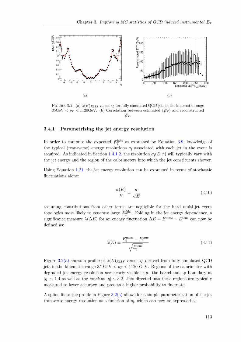
Chapter 3. Improving MC statistics of QCD induced instrumental /ET
η-4 -3 -2 -1 0 1 2 3 4
)G
eV
RM
S (
1
1.2
1.4
1.6
1.8
2
2.2
2.4
2.6
2.8
(a)
(GeV)MC
>missTEstimated <E
0 50 100 150 200 250 300
(G
eV
)m
iss
TR
eco
nstr
ucte
d E
0
50
100
150
200
(b)
Figure 3.2: (a) λ(E)RMS versus ηj for fully simulated QCD jets in the kinematic range35GeV < pT < 1120GeV. (b) Correlation between estimated 〈 /ET 〉 and reconstructed
/ET .
3.4.1 Parametrizing the jet energy resolution
In order to compute the expected /EfakeT as expressed by Equation 3.9, knowledge of
the typical (transverse) energy resolutions σj associated with each jet in the event is
required. As indicated in Section 1.4.1.2, the resolution σj(E, η) will typically vary with
the jet energy and the region of the calorimeters into which the jet constituents shower.
Using Equation 1.21, the jet energy resolution can be expressed in terms of stochastic
fluctuations alone:
σ(E)
E≡ a√
E(3.10)
assuming contributions from other terms are negligible for the hard multi-jet event
topologies most likely to generate large /EfakeT . Folding in the jet energy dependence, a
significance measure λ(∆E) for an energy fluctuation ∆E = Emeas − Etrue can now be
defined as:
λ(E) ≡Emeas
j − Etruej√
Etruej
(3.11)
Figure 3.2(a) shows a profile of λ(E)RMS versus ηj derived from fully simulated QCD
jets in the kinematic range 35 GeV < pT < 1120 GeV. Regions of the calorimeter with
degraded jet energy resolution are clearly visible, e.g. the barrel-endcap boundary at
|η| ∼ 1.4 as well as the crack at |η| ∼ 3.2. Jets directed into these regions are typically
measured to lower accuracy and possess a higher probability to fluctuate.
A spline fit to the profile in Figure 3.2(a) allows for a simple parameterization of the jet
transverse energy resolution as a function of ηj, which can now be expressed as:
113

Chapter 3. Improving MC statistics of QCD induced instrumental /ET
σj(Ej, ηj) = λ(E)RMS,j ×√Ej × sin(θj) (3.12)
where θj = 2 arctan (e−ηj) is the polar angle measured with respect to the beamline.
3.4.2 Expected /ET versus reconstructed /ET
With an η-dependent parameterization from which the expected jet energy resolutions
can be computed individually for each jet in the event, a generator level estimate for
the magnitude of the /ET can be expressed as a (scalar)3 sum of all real and fake contri-
butions:
〈 /ET 〉 =∑
/ET (ν) + 〈 /EfakeT 〉Njet (3.13)
where∑
/ET (ν) indicates a vectorial sum over all neutrino transverse momenta and
〈 /EfakeT 〉Njet is given by Equation 3.9.
The resulting correlation between the generator level estimate 〈 /ET 〉 and the actual
reconstructed /ET as computed by the reconstruction algorithm described in Section 3.1,
is shown in Figure 3.2(b). Because 〈 /ET 〉 is derived from the mean value of a probability
distribution, the estimation method is inherently susceptible to statistical fluctuations.
The reconstructed /ET will therefore often fall low of 〈 /ET 〉 . By the same token, events
with small 〈 /ET 〉 will occasionally fluctuate to produce large reconstructed /ET . Even so,
a correlation between 〈 /ET 〉 and reconstructed /ET is observed, the predictive power of
which enables a rough event categorization.
Figure 3.3 shows the reconstructed /ET spectrum in simulated QCD dijet events, along
with the subset of events flagged as belonging to either of the three categories: low
(〈 /ET 〉 < 50 GeV), intermediate (50 GeV< 〈 /ET 〉 < 100 GeV) and large (〈 /ET 〉 > 100
GeV).
While the method is susceptible to statistical fluctuations and the reconstructed /ETwill often be smaller than estimated at the generator level, the large majority of events
with /ET > 100 GeV are nevertheless seen to be appropriately categorized as large by
〈 /ET 〉. Upward fluctuations will push a small fraction of events flagged as intermediate
into the high tail of the reconstructed /ET spectrum. Such fluctuations are inherent to
the method and can scarcely be avoided. Finally, the tail is seen to contain a few events
flagged with a low probability of producing large /ET . These are principally single events
originating from low pT scattering bins and consequently given large scaling weights.
The large reconstructed /ET in these events is likely to derive from other sources than
jet fluctuations.
3A scalar summation, rather than a vectorial summation is employed because the expected fake con-tribution 〈 /Efake
T 〉 is a scalar quantity determined by way of the mean value of a probability distribution.While a vectorial summation would be more correct, a scalar summation has the additional benefit thatevents containing hard neutrinos buried in jets are weighted without regard to 〈 /Efake
T 〉, the latter ofwhich may be subject to substantial fluctuations.
114

Chapter 3. Improving MC statistics of QCD induced instrumental /ET
reconstructed (GeV)missTE
0 50 100 150 200 250 300 350 400 450 500
-1E
ven
ts / 1
0 G
eV
/ 1
0 f
b
1
10
210
310
410
510
610
710
810
910
1010
1110
1210miss
TCombined reconstructed E
< 50 GeVMC
>miss
TLow: <E
< 100 GeVMC
>miss
TIntermediate: 50 GeV < <E
> 100 GeVMC
>miss
TLarge: <E
Figure 3.3: /ET spectrum of simulated QCD dijets with subsets flagged with 〈 /ET 〉low, intermediate and high.
3.5 The method applied as a generator filter
The ability of the method to correctly flag particle level event configurations prone to
yield large reconstructed /ET , may be exploited in a generator filter. The application
of such a filtering mechanism early in the simulation chain described in Section 1.6
allows for a targeted population of the tail region of the reconstructed /ET -spectrum by
preferentially passing only those generated particle level event configurations prone to
furnish large reconstructed /ET through the full GEANT-based simulation. The resulting
filtered samples with enhanced tail statistics may then be combined with unfiltered
samples to significantly reduce statistical uncertainties across a broader kinematical
regime, a feature which in turn facilitates the development of more accurate search
strategies for new physics in channels involving large /ET .
3.5.1 Filter rejection and efficiency
The performance of the method when applied as a generator filter may be measured in
terms of its ability to:
(A) reject all uninteresting events, thereby reducing the effective cross section as far
as possible
(B) retain all events producing large reconstructed /ET
115
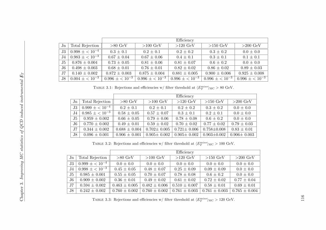
Ch
apte
r3.
Impro
vin
gM
Cst
ati
stic
sof
QC
Din
du
ced
inst
rum
enta
l/ET
Efficiency
Jn Total Rejection >80 GeV >100 GeV >120 GeV >150 GeV >200 GeV
J3 0.998 ± < 10−4 0.3 ± 0.1 0.2 ± 0.1 0.2 ± 0.2 0.3 ± 0.2 0.0 ± 0.0
J4 0.983 ± < 10−3 0.67 ± 0.04 0.67 ± 0.06 0.4 ± 0.1 0.3 ± 0.1 0.1 ± 0.1
J5 0.876 ± 0.004 0.73 ± 0.05 0.81 ± 0.06 0.81 ± 0.07 0.6 ± 0.2 0.0 ± 0.0
J6 0.498 ± 0.003 0.68 ± 0.01 0.76 ± 0.01 0.82 ± 0.02 0.86 ± 0.02 0.89 ± 0.03
J7 0.140 ± 0.002 0.872 ± 0.003 0.875 ± 0.004 0.881 ± 0.005 0.900 ± 0.006 0.925 ± 0.008
J8 0.004 ± < 10−3 0.996 ± < 10−3 0.996 ± < 10−3 0.996 ± < 10−3 0.996 ± < 10−3 0.996 ± < 10−3
Table 3.1: Rejections and efficiencies w/ filter threshold at 〈EmissT 〉MC > 80 GeV.
Efficiency
Jn Total Rejection >80 GeV >100 GeV >120 GeV >150 GeV >200 GeV
J3 0.999 ± < 10−4 0.2 ± 0.1 0.2 ± 0.1 0.2 ± 0.2 0.3 ± 0.2 0.0 ± 0.0
J4 0.985 ± < 10−3 0.58 ± 0.05 0.57 ± 0.07 0.3 ± 0.1 0.2 ± 0.1 0.0 ± 0.0
J5 0.959 ± 0.002 0.66 ± 0.05 0.79 ± 0.06 0.78 ± 0.08 0.6 ± 0.2 0.0 ± 0.0
J6 0.770 ± 0.002 0.49 ± 0.01 0.59 ± 0.02 0.70 ± 0.02 0.77 ± 0.02 0.79 ± 0.03
J7 0.344 ± 0.002 0.688 ± 0.004 0.702± 0.005 0.721± 0.006 0.758±0.008 0.83 ± 0.01
J8 0.096 ± 0.001 0.906 ± 0.001 0.905± 0.002 0.905± 0.002 0.903±0.002 0.906± 0.003
Table 3.2: Rejections and efficiencies w/ filter threshold at 〈EmissT 〉MC > 100 GeV.
Efficiency
Jn Total Rejection >80 GeV >100 GeV >120 GeV >150 GeV >200 GeV
J3 0.999 ± < 10−4 0.0 ± 0.0 0.0 ± 0.0 0.0 ± 0.0 0.0 ± 0.0 0.0 ± 0.0
J4 0.998 ± < 10−3 0.45 ± 0.05 0.48 ± 0.07 0.25 ± 0.09 0.09 ± 0.09 0.0 ± 0.0
J5 0.985 ± 0.001 0.55 ± 0.05 0.70 ± 0.07 0.78 ± 0.08 0.6 ± 0.2 0.0 ± 0.0
J6 0.909 ± 0.002 0.36 ± 0.01 0.49 ± 0.02 0.61 ± 0.02 0.72 ± 0.02 0.77 ± 0.04
J7 0.594 ± 0.002 0.463 ± 0.005 0.482 ± 0.006 0.510 ± 0.007 0.58 ± 0.01 0.69 ± 0.01
J8 0.242 ± 0.002 0.760 ± 0.002 0.760 ± 0.002 0.761 ± 0.003 0.761 ± 0.003 0.765 ± 0.004
Table 3.3: Rejections and efficiencies w/ filter threshold at 〈EmissT 〉MC > 120 GeV. 116

Chapter 3. Improving MC statistics of QCD induced instrumental /ET
Jn samples
1 2 3 4 5 6 7 8
Jn samples
1 2 3 4 5 6 7 8
Re
jec
tio
n
0
0.2
0.4
0.6
0.8
1
Figure 3.4: Filter rejections at three different filter thresholds: Λfilter > 80 GeV(red, triangles), Λfilter > 100 GeV (black, open circles) and Λfilter > 120 GeV (blue,
full circles).
Jn samples3 4 5 6 7 8
Eff
icie
nc
y
0
0.1
0.2
0.3
0.4
0.5
0.6
0.7
0.8
0.9
Figure 3.5: Filter efficiencies achieved with Λfiter > 100 GeV, evaluated at variousthresholds of reconstructed /ET : 80 GeV (red, circle), 100 GeV (blue, square), 120 GeV
(green, dot) and 200 GeV (black, triangle).
117

Chapter 3. Improving MC statistics of QCD induced instrumental /ET
Figure 3.4 shows the total rejections and efficiencies obtained on simulated QCD dijets
in various bins of hard scattering pT , when the method is applied as a generator filter
with 〈 /ET 〉 > Λfilter.
The rejection Rfilter is herein defined as
Rfilter =Ngen −Npassed
gen
Ngen(3.14)
where Npassedgen is the number of events passing the filter from a total of Ngen generated
events. The accuracy of the filtering procedure is herein measured by the filter efficiency:
εfilter =Npassed
gen ( /ET > Λfilter)
Ngen( /ET > Λfilter)(3.15)
where the numerator and denominator indicate the fraction of events with reconstructed
/ET above the filter threshold Λfilter, in the filtered subset and the total sample, respec-
tively.
With a filter threshold of Λfilter = 100 GeV, Figure 3.4 indicates that rejections in excess
of 90% are achieved in the intermediate bins of hard scattering pT (140 GeV-560 GeV),
consequently reducing the effective cross section by 1-2 orders of magnitude. In the bin
beyond (560 GeV< pT <1120 GeV), a rejection of ∼ 75% is achieved, corresponding to
a factor 4 reduction in the effective cross section.
The corresponding efficiencies are shown in Figure 3.5, from which efficiencies between
60% - 80% are observed across the central bins 140 GeV < pT < 1120 GeV. In the case
of the upper bin (560 GeV < pT < 1120 GeV), in which a tail extends well beyond
reconstructed /ET > 100 GeV, Table 3.2 indicates that efficiencies of roughly 70% and
80% are obtained above a reconstructed /ET of 120 GeV and 200 GeV, respectively.
As indicated in Figure 3.3, events with reconstructed /ET> 100 GeV failing filter capture
are typically flagged with 〈 /ET 〉 in the intermediate range. A lowering of Λfilter will
therefore improve filter efficiencies, albeit at the expense of lower filter rejections. Table
3.1 indicates that a lowering of the filter threshold will impact the efficiency-rejection
trade-off in the various bins of hard scattering pT differently. By way of example, a 15 %
efficiency improvement against a marginal 0.2% fall in rejection is achieved in the lower
central scattering bin (140 GeV-280 GeV) in the region of reconstructed /ET> 100 GeV
by lowering the filter threshold Λfilter from 100 GeV to 80 GeV. In the upper central
bin (560 GeV-1120 GeV) by contrast, an efficiency improvement of roughly 30 % is
achieved, but only at the cost of a non-negligible 35% reduction in the total rejection.
In practical terms, the most appropriate filter threshold Λfilter will therefore depend on
the kinematic region of choice and the desired efficiency-rejection trade-off.
118
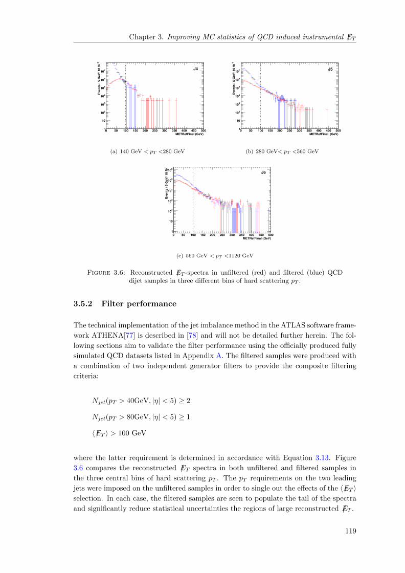
Chapter 3. Improving MC statistics of QCD induced instrumental /ET
METRefFinal (GeV)0 50 100 150 200 250 300 350 400 450 500
-1E
ven
ts / 5
GeV
/ 10 f
b
1
10
210
310
410
510
610
710J4
(a) 140 GeV < pT <280 GeV
METRefFinal (GeV)0 50 100 150 200 250 300 350 400 450 500
-1E
ven
ts / 5
GeV
/ 10 f
b
1
10
210
310
410
510
610
710J5
(b) 280 GeV< pT <560 GeV
METRefFinal (GeV)0 50 100 150 200 250 300 350 400 450 500
-1E
ven
ts / 5
GeV
/ 10 f
b
1
10
210
310
410
510
610
J6
(c) 560 GeV < pT <1120 GeV
Figure 3.6: Reconstructed /ET -spectra in unfiltered (red) and filtered (blue) QCDdijet samples in three different bins of hard scattering pT .
3.5.2 Filter performance
The technical implementation of the jet imbalance method in the ATLAS software frame-
work ATHENA[77] is described in [78] and will not be detailed further herein. The fol-
lowing sections aim to validate the filter performance using the officially produced fully
simulated QCD datasets listed in Appendix A. The filtered samples were produced with
a combination of two independent generator filters to provide the composite filtering
criteria:
Njet(pT > 40GeV, |η| < 5) ≥ 2
Njet(pT > 80GeV, |η| < 5) ≥ 1
〈 /ET 〉 > 100 GeV
where the latter requirement is determined in accordance with Equation 3.13. Figure
3.6 compares the reconstructed /ET spectra in both unfiltered and filtered samples in
the three central bins of hard scattering pT . The pT requirements on the two leading
jets were imposed on the unfiltered samples in order to single out the effects of the 〈 /ET 〉selection. In each case, the filtered samples are seen to populate the tail of the spectra
and significantly reduce statistical uncertainties the regions of large reconstructed /ET .
119

Chapter 3. Improving MC statistics of QCD induced instrumental /ET
jetN0 2 4 6 8 10 12 14 16 18 20
No
rma
lize
d t
o u
nity
0
0.05
0.1
0.15
0.2No cuts
Jet multiplicity
(a) No cuts
jetN0 2 4 6 8 10 12 14 16 18 20
No
rma
lize
d t
o u
nity
0
0.05
0.1
0.15
0.2
0.25
0.3SUSY cuts
Jet multiplicity
(b) SUSY cuts
Figure 3.7: A comparison of the jet multiplicity in events from J5 (280 GeV< pT <560GeV) with reconstructed /ET>100 GeV, in unfiltered (blue, solid circle) and in filtered(red, empty circle) samples. In (a) no additional selection cuts are applied, in (b)
typical SUSY selection cuts are applied.
3.5.3 Event kinematics in filtered events
The reconstructed event kinematics in filtered and unfiltered samples will naturally
differ. With no further selection cuts applied, events from filtered samples with re-
constructed /ET > 100 GeV will tend towards higher jet multiplicities and harder jet
transverse momenta, as shown in Figure 3.7(a), as such event configurations are more
likely to exhibit a greater degree of imbalance and hence produce larger /EfakeT estimates.
Differences in event kinematics should however be duly considered within the context
of the analysis in which the filtered samples are applied. Any differing behaviour in
filtered events that are rejected by the basic selection criteria of the online trigger or
offline selection is clearly of no consequence for the remaining analysis.
In order to compare unfiltered and filtered events within the context of a generic ATLAS
inclusive supersymmetry search, the following selection was applied to both unfiltered
and filtered samples [79]:
/ET > 100 GeV and Njet ≥ 4
pjet 1T > 100 GeV and pjet 2,3,4
T > 50 GeV
transverse sphericity ST4 > 0.2
lepton veto
4The transverse sphericity ST ≡ 2λ2λ1+λ2
is defined in terms of the eigenvalues λ1, λ2 of the transverse
sphericity tensor Sx,y =
(p
(i)x p
(i)x p
(i)x p
(i)y
p(i)x p
(i)y p
(i)y p
(i)y
)
120

Chapter 3. Improving MC statistics of QCD induced instrumental /ET
(GeV)TP0 200 400 600 800 1000 1200 1400
No
rma
lize
d t
o u
nity
0
0.01
0.02
0.03
0.04
0.05
0.06
0.07
No cuts
Jet 1
(GeV)TP0 200 400 600 800 1000 1200 1400
No
rma
lize
d t
o u
nity
0
0.02
0.04
0.06
0.08
0.1
0.12
0.14
0.16
0.18
0.2
0.22
0.24
SUSY cuts
Jet 1
(GeV)TP0 200 400 600 800 1000 1200 1400
No
rma
lize
d t
o u
nity
0
0.01
0.02
0.03
0.04
0.05
0.06
0.07
No cuts
Jet 2
(GeV)TP0 200 400 600 800 1000 1200 1400
No
rma
lize
d t
o u
nity
0
0.02
0.04
0.06
0.08
0.1
0.12
0.14
0.16
0.18
0.2
SUSY cuts
Jet 2
Figure 3.8: Transverse momentum spectra of the two leading jets in events from J5(280 GeV< pT <560 GeV) with reconstructed /ET> 100 GeV, in unfiltered (blue, solidcircle) and in filtered (red, empty circle) samples. Left: no additional cuts applied.
Right: typical SUSY selection cuts applied.
Figures 3.7(b) and 3.8 indicate that the tendency towards higher jet multiplicities and
larger transverse momenta is largely alleviated by the above selection. It was also found
that events which were wrongfully rejected by the filtering method would also tend to
fail the above selection cuts [78].
3.6 Summary
Proper understanding of event /ET is crucial for the discovery of many new physics
scenarios at the LHC. As a particular case in point, R-parity conserving supersymmetry
scenarios are typically characterised by large /ET signatures, making proper control of
all backgrounds faking large /ET an important prerequisite for discovery. In this context,
fluctuating QCD jets pose a particular challenge, one further aggravated by very large
cross sections.
This chapter introduced a probabilistic method to attain a generator level estimate of
instrumental contributions to reconstructed /ET originating from jet fluctuations in the
calorimeters. The method accounts for detector resolution effects through a parametriza-
tion derived from fully simulated data. The estimated fake contributions are then com-
bined with the true /ET from non-interacting particles to yield an estimate for the total
expected /ET in the event.
121
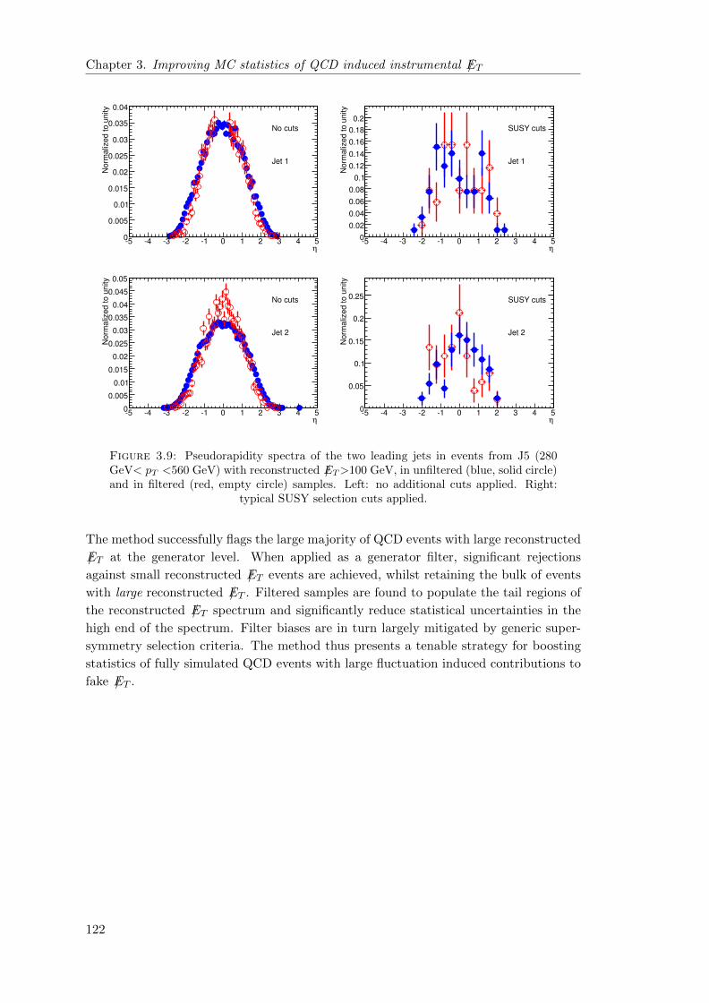
Chapter 3. Improving MC statistics of QCD induced instrumental /ET
η-5 -4 -3 -2 -1 0 1 2 3 4 5
No
rma
lize
d t
o u
nity
0
0.005
0.01
0.015
0.02
0.025
0.03
0.035
0.04
No cuts
Jet 1
η-5 -4 -3 -2 -1 0 1 2 3 4 5
No
rma
lize
d t
o u
nity
0
0.02
0.04
0.06
0.08
0.1
0.12
0.14
0.16
0.18
0.2
SUSY cuts
Jet 1
η-5 -4 -3 -2 -1 0 1 2 3 4 5
No
rma
lize
d t
o u
nity
0
0.005
0.01
0.015
0.02
0.025
0.03
0.035
0.04
0.045
0.05
No cuts
Jet 2
η-5 -4 -3 -2 -1 0 1 2 3 4 5
No
rma
lize
d t
o u
nity
0
0.05
0.1
0.15
0.2
0.25 SUSY cuts
Jet 2
Figure 3.9: Pseudorapidity spectra of the two leading jets in events from J5 (280GeV< pT <560 GeV) with reconstructed /ET>100 GeV, in unfiltered (blue, solid circle)and in filtered (red, empty circle) samples. Left: no additional cuts applied. Right:
typical SUSY selection cuts applied.
The method successfully flags the large majority of QCD events with large reconstructed
/ET at the generator level. When applied as a generator filter, significant rejections
against small reconstructed /ET events are achieved, whilst retaining the bulk of events
with large reconstructed /ET . Filtered samples are found to populate the tail regions of
the reconstructed /ET spectrum and significantly reduce statistical uncertainties in the
high end of the spectrum. Filter biases are in turn largely mitigated by generic super-
symmetry selection criteria. The method thus presents a tenable strategy for boosting
statistics of fully simulated QCD events with large fluctuation induced contributions to
fake /ET .
122
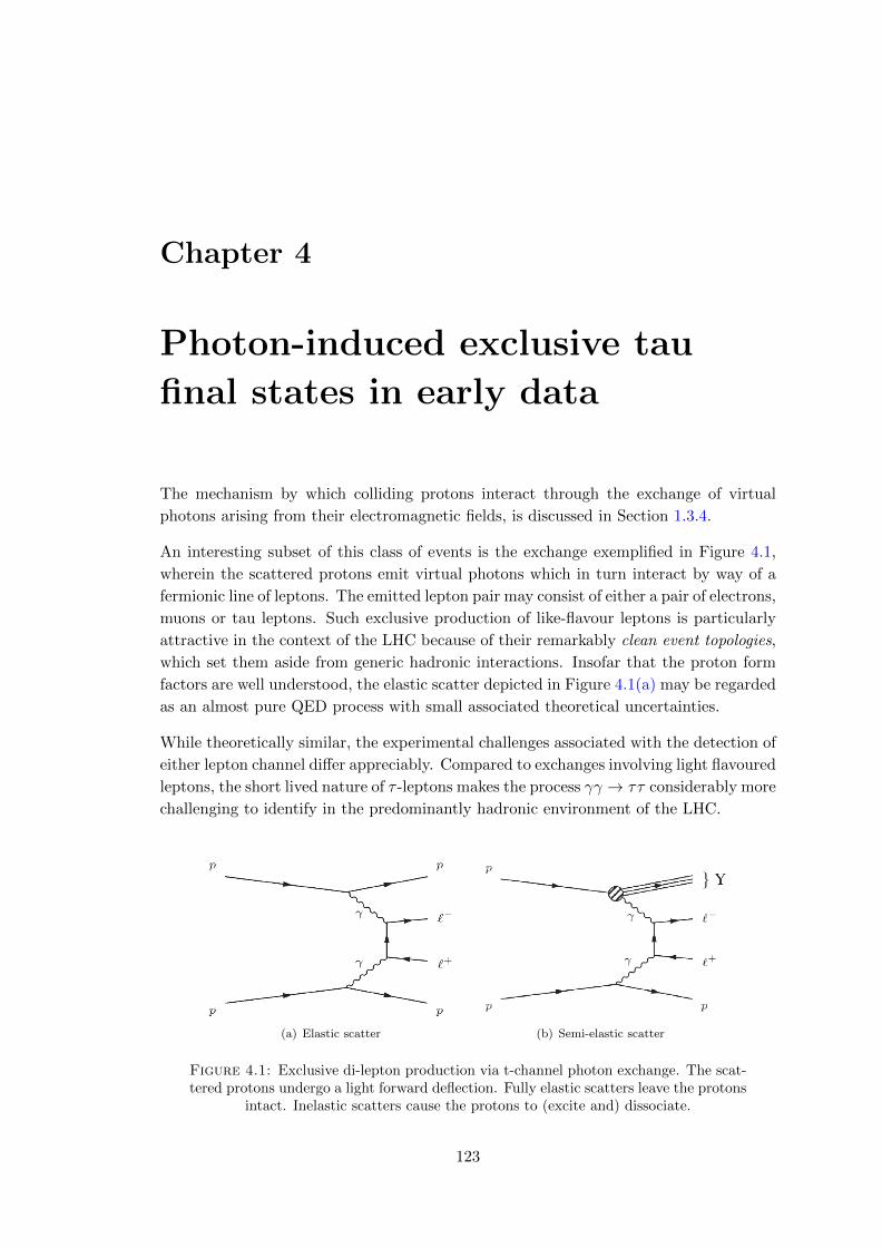
Chapter 4
Photon-induced exclusive tau
final states in early data
The mechanism by which colliding protons interact through the exchange of virtual
photons arising from their electromagnetic fields, is discussed in Section 1.3.4.
An interesting subset of this class of events is the exchange exemplified in Figure 4.1,
wherein the scattered protons emit virtual photons which in turn interact by way of a
fermionic line of leptons. The emitted lepton pair may consist of either a pair of electrons,
muons or tau leptons. Such exclusive production of like-flavour leptons is particularly
attractive in the context of the LHC because of their remarkably clean event topologies,
which set them aside from generic hadronic interactions. Insofar that the proton form
factors are well understood, the elastic scatter depicted in Figure 4.1(a) may be regarded
as an almost pure QED process with small associated theoretical uncertainties.
While theoretically similar, the experimental challenges associated with the detection of
either lepton channel differ appreciably. Compared to exchanges involving light flavoured
leptons, the short lived nature of τ -leptons makes the process γγ → ττ considerably more
challenging to identify in the predominantly hadronic environment of the LHC.
(a) Elastic scatter (b) Semi-elastic scatter
Figure 4.1: Exclusive di-lepton production via t-channel photon exchange. The scat-tered protons undergo a light forward deflection. Fully elastic scatters leave the protons
intact. Inelastic scatters cause the protons to (excite and) dissociate.
123

Chapter 4. Photon-induced exclusive tau final states in early data
In the following, a simulation study is presented which aims to evaluate the feasibility
of detecting photon induced di-lepton final states during the early phase of ATLAS
operation. After a brief introduction to two-photon physics at the LHC, an overview
of expected cross sections and event kinematics as predicted by Monte Carlo simulation
tools is provided. This is followed by a discussion of the experimental challenges which
serve to complicate an offline selection alongside any assumptions made in the analysis. It
is shown, that a common challenge in all three channels (e, µ, τ) is ineffective triggering.
To this end a dedicated trigger strategy has been developed and implemented which
offers early sensitivity to generic exclusive lepton final states. Drawing on these dedicated
triggers, the offline selection potential in the experimentally most challenging process
γγ → ττ is evaluated and results summarized for an integrated luminosity corresponding
to 100 pb−1.
4.0.1 Two-photon physics at other collider facilities
Exclusive di-lepton production as per mechanisms equivalent to those depicted in Figure
4.1, have been observed and studied by experiments at various other collider facilities in
the past. These include the electron-positron collider LEP, the electron-proton collider
HERA and more recently also the the heavy ion collider RHIC, as well as the proton-
antiproton collider TEVATRON. Their continued study at a proton-proton collider such
as the LHC is therefore warranted as a natural extension of a long existing programme.
The observation of photon induced lepton final states long remained elusive in hadron-
hadron collisions. The production cross sections at early hadron colliders such as CERN’s
ISR (proton-proton) and SppS (proton-antiproton), were too minute for potential de-
tection. A recent observation (2006) of exclusive di-leptons by the CDF(II) experi-
ment at TEVATRON (√s = 1.96 TeV), therefore marked the first of its kind at a
hadron collider facility. The experiment measured a cross section of σET>5GeV,|η|<2excl ee =
1.6+0.5−0.3(stat)± 0.3(sys) pb, corresponding to 16 exclusive e+e− candidates over a back-
ground expectation of 1.9 ± 0.3 events at an integrated luminosity of 532 pb−1, where
both cross section and kinematic distributions were found to agree well with theoretical
predictions [80].
This measurement confirms the observability of two-photon interactions in hadron col-
lider environments at TeV energies and partially warrants studies into applications at
the LHC where production rates are expected to increase significantly.
While the process γγ → ττ has been observed and studied at LEP [81] and HERA [82],
its observation remain elusive at hadron colliders at the time of writing. An observation
of this process at the LHC would therefore potentially be the first of its kind at a hadron
collider.
4.0.2 Early two-photon physics at the LHC
As a sizable fraction of pp collisions at the LHC will involve photon exchange interactions,
the LHC may to some extent be considered both a γγ and a γp collider. As discussed
124

Chapter 4. Photon-induced exclusive tau final states in early data
in Section 1.3.4, photon exchange interactions at the LHC are unique in that they may
occur at energies in excess of the electroweak scale, thereby opening for searches and
measurements of new physics coupling to photons [83]. While the effective luminosity
of such collisions is relatively modest, the reward is better understood initial conditions
and remarkably clean event topologies. This is especially true of elastic two-photon
processes and consequently studies into their physics potential is currently receiving
renewed attention.
All flavours of the process γγ → ll will arguably form important control samples for
searches for new physics by exclusive production mechanism. In addition, various pro-
posals have been made for possible applications of photon induced dilepton processes at
the LHC. These include:
• Lepton reconstruction studies: the absence of hadronic debris provides a
unique setting in which to investigate the lepton reconstruction performance at
low energies.
• Absolute luminosity measurements: the relatively large and well known cross
section (O(1%)) of the process γγ → µµ, makes it an intriguing candidate for
absolute luminosity measurements at the LHC [26, 84–86]. This is particularly
true in the early phase of operation when the machine luminosity is low and pile-
up effects negligible. (In principle, the process γγ → ee could be applied to the
same ends, however the comparative ease with which soft muons can be identified
renders the muon channel more favourable to this end).
• Calibration of very forward detector systems: from a measurement of the
pseudorapidities and invariant mass of the dilepton system, the interacting photon
energies can be estimated in the colinear approximation. Such a measurement is
tantamount to an estimation of the proton energy lossEγ
Eproton, which in turn can be
used to calibrate and align very forward detector systems such as those described
in Section 1.4.2.5 [87][26].
The range of applications available with exclusive di-tau processes naturally depends
on the success with which such events can be selected at the LHC. While theoretically
similar to the light flavour lepton channels, this process differs considerably in terms of
its experimental detection and measurement. Tau leptons decay as detailed in Chapter
2, leaving neutrinos in their wake which alter the kinematic balance of the di-tau system.
The escaping neutrinos also serve to reduce the effective cross section for τ -leptons in
the detectable kinematic range, a challenge further compounded by the predominantly
hadronic decay modi of the τ , making it harder to set apart in the hadronic environment
of the LHC.
The detection of the process γγ → ττ is therefore in many ways a considerable experi-
mental challenge in itself, and a confirmation of this process in early LHC data would
not only be an important confirmation of Standard Model physics, but also serve as a
vindication of the experimental capabilities of the ATLAS detector (potentially paving
the way for more exotic searches in exclusive channels).
125
Chapter 4. Photon-induced exclusive tau final states in early data
The striking simplicity of these events set them apart in an LHC context and may
compensate for comparatively modest cross sections. For early τ -lepton reconstruction
studies, this may prove to be an important supplement to more standard processes such
as Z(+jets)→ ττ andW (+jets)→ τντ . While such processes arguably enjoy higher pro-
duction rates and well constrained kinematics, their event topologies are more involved
and complex by comparison. Moreover, as discussed in Section 1.3 their production
cross sections and kinematics are subject to uncertainties in both non-perturbative QCD
effects and in the parton distribution functions of the colliding protons. The presence of
additional jets (V+ jets), further necessitates a dependence on a proper understanding
of the jet energy scale [32].
The almost pure QED nature of exclusive di-lepton processes make them relatively im-
mune to the uncertainties of QCD induced physics. As such they may prove a useful
complement to existing validation processes, such as gauge boson production. Because
the cross section is strongly peaked at low values of lepton transverse momentum, the
process γγ → ττ gives complementary access to a kinematic domain otherwise only
available in the tails of the transverse momentum spectra of leptonic decays of heavy
gauge bosons. Two-photon processes therefore offer an opportunity to collect a strik-
ingly clean sample of τ -candidate around the sensitivity threshold of current τ -lepton
reconstruction and identification tools in ATLAS. Such a sample may be used to shed
light on the performance of the tau reconstruction in the extreme low-energy regime, an
insight that may prove valuable in searches for new physics, such as e.g. certain SUSY
searches where the presence of very low energetic τ -leptons is prolific and an efficient
reconstruction and identification critical for the measurement of model parameters [52]
The cleanliness of exclusive events may potentially also make them attractive for studies
into tau substructure identification performance in current reconstruction algorithms and
provide a unique testbed for new and improved identification techniques. An overlay
with a QCD rich sample may help uncover effects of the underlying event in a controlled
manner.
4.1 Monte Carlo simulations and event characteristics
4.1.1 Monte Carlo simulations
All simulations of the exclusive two-photon process γγ → ll employed in this study were
performed with the event generator LPAIR [88, 89]. LPAIR performs a leading order
Matrix Element calculation of the process γγ → ll. The production cross section is then
computed as a convolution of the virtual photon fluxes and the cross section derived
from the matrix element calculation. LPAIR will also correctly account for the changing
kinematics of the di-lepton system expected in highly virtual photon exchanges. Elastic,
semi-elastic and fully inelastic scatters simulated by LPAIR therefore yield different
kinematic spectra. The hadronisation of the dissociated protons is not handled by
LPAIR, and consequently not treated herein. The implications of this omission is further
discussed in Section 4.2.2.
126
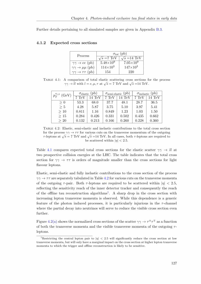
Chapter 4. Photon-induced exclusive tau final states in early data
Further details pertaining to all simulated samples are given in Appendix B.3.
4.1.2 Expected cross sections
Processσtot (pb)√
s =7 TeV√s =14 TeV
γγ → ee (pb) 5.48×10⁹ 7.05×10⁹
γγ → µµ (pb) 114×103 147×103
γγ → ττ (pb) 154 220
Table 4.1: A comparison of total elastic scattering cross sections for the processγγ → ll with l = e, µ, τ at
√s = 7 TeV and
√s =14 TeV.
pτ1,2T (GeV)
σelastic (pb) σsemi-elastic (pb) σinelastic (pb)7 TeV 14 TeV 7 TeV 14 TeV 7 TeV 14 TeV
≥ 0 53.3 68.0 37.7 48.1 28.7 36.5≥ 5 4.28 5.87 3.75 5.10 3.97 5.41≥ 10 0.811 1.16 0.849 1.23 1.03 1.50≥ 15 0.284 0.426 0.331 0.502 0.435 0.662≥ 20 0.132 0.213 0.166 0.260 0.228 0.360
Table 4.2: Elastic, semi-elastic and inelastic contributions to the total cross sectionfor the process γγ → ττ for various cuts on the transverse momentum of the outgoingτ -leptons at
√s = 7 TeV and
√s =14 TeV. In all cases, both τ -leptons are required to
be scattered within |η| < 2.5.
Table 4.1 compares expected total cross sections for the elastic scatter γγ → ll at
two prospective collision energies at the LHC. The table indicates that the total cross
section for γγ → ττ is orders of magnitude smaller than the cross sections for light
flavour leptons.
Elastic, semi-elastic and fully inelastic contributions to the cross section of the process
γγ → ττ are separately tabulated in Table 4.2 for various cuts on the transverse momenta
of the outgoing τ -pair. Both τ -leptons are required to be scattered within |η| < 2.5,
reflecting the sensitivity reach of the inner detector tracker and consequently the reach
of the offline tau reconstruction algorithms1. A sharp drop in the cross section with
increasing lepton transverse momenta is observed. While this dependence is a generic
feature of the photon induced processes, it is particularly injurious in the τ -channel
where the partial decay into neutrinos will serve to reduce the visible cross section even
further.
Figure 4.2(a) shows the normalized cross sections of the scatter γγ → τ±τ∓ as a function
of both the transverse momenta and the visible transverse momenta of the outgoing τ -
leptons.
1Restricting the central lepton pair to |η| < 2.5 will significantly reduce the cross section at lowtransverse momenta, but will only have a marginal impact on the cross section at higher lepton transversemomenta to which the trigger and offline reconstruction is likely to be sensitive.
127
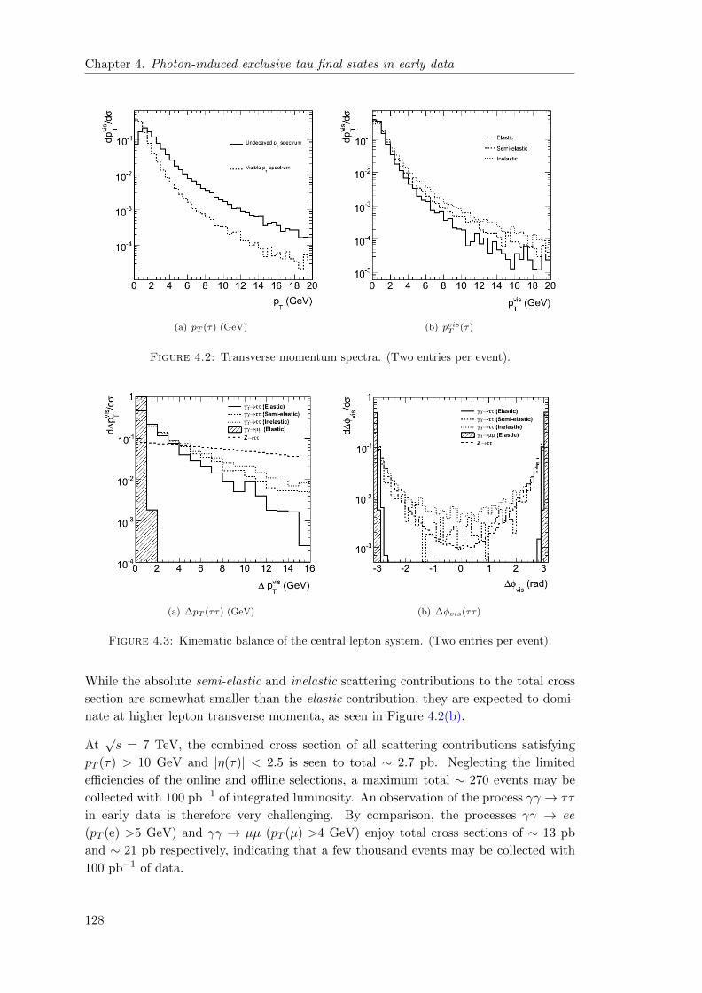
Chapter 4. Photon-induced exclusive tau final states in early data
(a) pT (τ) (GeV) (b) pvisT (τ)
Figure 4.2: Transverse momentum spectra. (Two entries per event).
(a) ∆pT (ττ) (GeV) (b) ∆φvis(ττ)
Figure 4.3: Kinematic balance of the central lepton system. (Two entries per event).
While the absolute semi-elastic and inelastic scattering contributions to the total cross
section are somewhat smaller than the elastic contribution, they are expected to domi-
nate at higher lepton transverse momenta, as seen in Figure 4.2(b).
At√s = 7 TeV, the combined cross section of all scattering contributions satisfying
pT (τ) > 10 GeV and |η(τ)| < 2.5 is seen to total ∼ 2.7 pb. Neglecting the limited
efficiencies of the online and offline selections, a maximum total ∼ 270 events may be
collected with 100 pb−1 of integrated luminosity. An observation of the process γγ → ττ
in early data is therefore very challenging. By comparison, the processes γγ → ee
(pT (e) >5 GeV) and γγ → µµ (pT (µ) >4 GeV) enjoy total cross sections of ∼ 13 pb
and ∼ 21 pb respectively, indicating that a few thousand events may be collected with
100 pb−1 of data.
128

Chapter 4. Photon-induced exclusive tau final states in early data
4.1.3 Event kinematics
The kinematics of exclusive di-lepton events are characterized by a well balanced di-
lepton system, both in transverse momentum (∆pT (l±, l∓)) and acoplanarity (∆φ(l+, l−)).
Figure 4.3 compares the balance of the visible di-tau system with that of an exclusive
di-muon system in both of these quantities. The decay of either τ -lepton is seen to dis-
tort the a priori perfect balance in the di-tau system, as is reflected in the broadening of
the ∆pvisT and ∆φvis spectra. Even so, the absence of additional gluon radiation is seen
to furnish a comparatively well balanced visible di-tau system when contrasted with the
balance in Z → ττ . Despite a relative deterioration when compared to the light flavour
lepton channels, the balance of the visible di-tau system will therefore still prove to be
a useful characteristic to exploit in the offline event selection.
4.2 A note on the experimental challenges and assump-
tions made
4.2.1 Event reconstruction and background suppression
At the very onset, the observation of the process γγ → ττ appears more challenging
to detect than its light flavour counterparts. For one, the soft nature of the scattered
leptons in photon induced processes is more damaging in the τ -channel, because the
sensitivity reach of the reconstruction and identification of τ -leptons typically does not
extend to such low values of transverse momentum as is the case for e± and µ±. The
problem is further exacerbated by the decay into neutrinos which reduces the fraction
of the total τ -momentum available for experimental detection and distorts the balance
in the di-tau system. Because both online and offline τ -reconstruction tools are most
sensitive to the higher end of the di-tau transverse momentum spectrum, any search
will necessarily be susceptible to the theoretical uncertainties in the cross sections of
semi-elastic and inelastic scatters.
The challenges of the τ -channel must also be viewed in light of the experimental climate
of the LHC. Since the rate at which strong interactions occur far exceeds that of photon
interactions, an accurate and efficient identification mechanism is essential to extract
signal events from the overwhelming number of background events prone to mimic the
signal signatures. Because both τ -leptons are very likely to decay hadronically, the
signal will mostly appear strikingly similar to more prolific QCD-induced exclusive jet
processes. Other potential backgrounds are discussed in Section 4.5.
4.2.2 Rapidity gaps and proton dissociation
A hallmark of exclusive two-photon events is the absence of activity to either side of the
central system. Such an empty region of the detector will hence be referred to as a large
rapidity gap. Exclusive elastic scatters should therefore always contain two large rapidity
129

Chapter 4. Photon-induced exclusive tau final states in early data
(a) (b)
Figure 4.4: (a) The |η|-spectrum of forward scattered debris in semi-elastic γγ inter-actions. (b) The |η| versus energy of the most central proton dissociation product in a√
s = 7 TeV semi-elastic scatter.
gaps, a feature which stands in stark contrast to events where the hard scatter breaks
the proton apart and sends the proton remnant into the forward region of the central
detector. Properly identified rapidity gaps, are therefore powerful tools to suppress the
bulk of hadronic interactions. A robust identification in turn rests on proper control of
all physical and instrumental effects that may destroy the rapidity gaps.
Highly virtual photon emissions may excite the photon emitting proton and cause it
to dissociate. Table 4.2 indicates that scatters involving τ -leptons with pT > 10 GeV
typically involve proton dissociation and consequently a non-zero probability that the
rapidity gap is polluted by remnants of the dissociative system. However, because√sγγ
√spp the dissociative system carries a large forward boost and will most likely
escape undetected through the beam pipe. While proton debris might well appear in the
very forward detector systems, the rapidity gaps in the central detector maintain a high
probability of remaining intact. This is confirmed by the spectrum in Figure 4.4(a) in
which the |η|-distribution of proton debris particles in semi-elastic γγ-scatters is shown,
as predicted by the MBR Monte Carlo [90]2. The probability of rapidity gaps remain-
ing intact in face of proton dissociation is seen to be very large. It is also noteworthy
that debris particles scattered into the central detector region are very unlikely to have
energies in excess of a few GeV, as indicated by Figure 4.4(b).
For this reason, this analysis assumes that the dissociative system in semi-elastic and
inelastic scatters is always deflected at such small angles with respect to the beam
pipe, that rapidity gaps are preserved and the events in the central detector appear
indistinguishable from elastic scatters.
2The dissociation kinematics are provided by the fragment cluster function of the Minimum BiasRockefeller (MBR) Monte Carlo, in which the proton is fragmented into pions based on the kinematicinput from LPAIR. The pions are then boosted back to the laboratory frame. I am indebted to A.Hamilton for providing the necessary code fragments.
130

Chapter 4. Photon-induced exclusive tau final states in early data
4.2.3 Event pile-up
As discussed in Section 1.3.6, nominal luminosity running will see each hard scatter
accompanied by several additional scatters taking place between other protons in the
same bunch crossing. This effect is known as event pile-up and will typically result
in several additional tracks and calorimeter hits in the central detector that bare no
relation to the exclusive signal. Pile-up events are therefore potentially devastating to a
search for exclusive photon induced processes, because the probability that rapidity gaps
survive in the presence of pile-up is low. However, as discussed in Section 1.3.6, event
pile-up in the early phases of LHC running is expected to be small. Consequently, pile-
up effects will be neglected in this analysis. The challenge will therefore be to observe a
signal and collect as large a sample as possible with low-luminosity data where pile-up
effects are negligible.
4.2.4 Proton tagging with forward detectors
A commonly proposed method of dicerning exclusive photon interactions involves the
use of forward proton tagging, where an attempt is made to identify the photon emitting
protons in the very forward detector systems. Following the elastic emission of a photon,
the unbroken proton is only lightly deflected and exits the central detector through the
beam pipe along with the spectator protons of the beam. However, the slight loss in
energy following the photon emission results in a larger deflection in the beam magnetic
field and facilities a detection in near-beam detectors positioned at a large distance
from the interaction point. While such techniques provide a potent means of tagging
two-photon interaction processes even in the face of pile-up, the proton tagging devices
discussed in Section 1.4.2.5 will not be available during early LHC operation. They will
therefore not be considered in this study.
4.2.5 Trigger
Finally, an event is not available for offline selection if it does not pass the ATLAS L1
and HLT triggers. The enormous rates at which soft QCD interactions occur at the
LHC severely restricts the extent to which ATLAS can afford to trigger on hadronic
objects with low transverse momenta. Low energetic hadronically decaying τ -leptons
can therefore only be triggered in conjunction with large prescales3 which serve to keep
trigger rates within required limits. Large prescales however, do not allow for efficient
triggering on relatively rare processes such as γγ → ll. A central challenge for this
analysis, and a prerequisite for an observation of the process γγ → ττ in early data, is
therefore to find an efficient means of triggering on the signal at minimal cost to the
overall trigger rate.
3Prescales are introduced as a means of reducing the number of events passing a given trigger chain.The prescale factor dictates the rate at which events satisfying the trigger criteria will be accepted. Aprescale factor of 1000 signifies that only 1 in 1000 events satisfying the trigger criteria will be accepted.Prescales with different factors can be applied at all levels of the trigger chain.
131

Chapter 4. Photon-induced exclusive tau final states in early data
4.3 The online selection of exclusive lepton final states
As explained in Section 1.5, any collision event is required to pass both the L1 trigger
and the HLT triggers before the recorded data are made available for more detailed
offline analysis. The soft nature of photon-induced di-lepton final states makes them
particularly challenging processes to trigger on. As discussed in Chapter 2, this is espe-
cially true of the process γγ → τhadτhad, because hadronically decaying taus often leave
more ambiguous and complicated signatures in the detector. The need to make a rapid
decision on the basis of the comparatively crude information available will necessarily
limit the ability of the L1 trigger to recognise tau signatures, a challenge further com-
pounded by the necessity of keeping the enormous background rates within tolerable
limits. At low transverse momenta, these challenges are typically met by either rais-
ing the threshold on the trigger objects or by applying suitable prescale factors to the
trigger decision or indeed a combination of both. As is explained below, both strategies
are detrimental to the efficiency of triggering on the signal, which is characterised by a
comparatively modest cross-section falling quickly with the pT of the outgoing lepton
pair.
In the following, the shortcomings of default trigger chains in ATLAS with the respect
to the process γγ → ll are discussed, before a dedicated trigger strategy is developed
which aims to target lepton final states from all exclusive sources.
4.3.1 Prospects with default triggers
While the ATLAS trigger chains are designed to retain sensitivity to a variety of different
final states at a range of different energy scales, they typically target particle objects
at higher transverse momenta than is characteristic of photon induced processes. The
relatively high thresholds on the lowest energy leptons triggers is indicative of this fact.
Table 4.3 lists the lowest threshold lepton trigger chains available in the first draft trigger
menu designed for deployment at L ∼ 1031cm−2s−1 along with projected prescales. It
also lists the efficiencies of these chains on various γγ → ll processes with respect to the
minimal offline selection criterion that leptons of the appropriate flavour as defined in
Section 4.4 be reconstructed4.
It should be noted that the ATLAS trigger menus are in flux and are continuously
modified to best meet the needs of the collaboration in a given luminosity scenario
provided by the LHC machine. In particular, early running at instantaneous luminosities
< 1031cm−2s−1 may well see ATLAS operate with lower prescales than reported herein.
The configurations detailed in the following are all based on the draft menu for operation
at 1031cm−2s−1 [32][91] which were valid at the time when the studies presented herein
were conducted.
4In the tau channel, only one hadronic tau candidate is required. In the electron (muon) channel,two reconstructed electrons (muons) are required.
132

Chapter 4. Photon-induced exclusive tau final states in early data
Lepton flavour Signature L1 item Prescales (L1-L2-EF) Efficiency
ε (γγ → τhadτhad)
TaustauNoCut L1_TAU5 10000000-1-1 60%
tau12_loose L1_TAU6 1-10-750 13%tau16_loose L1_TAU9 1-600-1 9%
ε (γγ → ee)
Electronse5_medium L1_EM3 60-1-1 82%e10_medium L1_EM7 1-1-1 18%2e5_medium L1_2EM3 1-1-1 43%
ε (γγ → µµ)
Muons
mu4 L1_MU4 1-5-300 84%mu6 L1_MU6 1-1-30 38%2mu4 L1_2MU4 1-1-1 45%
mu4_mu6 L1_2MU4_MU6 1-1-1 28%
Table 4.3: Lowest threshold lepton triggers for operation at L ∼ 1031cm−2s−1 withtheir (unprescaled) efficiencies on γγ → ll. A minimal object selection as defined inSection 4.4 is applied to offline reconstructed leptons. The samples satisfy the generator
selections: pT (τhad)>10 GeV, pT (e) > 5 GeV and pT (µ) > 4 GeV.
Taus
As indicated by Table 4.3, the lowest threshold tau triggers are all assigned high prescales
rendering them unsuitable for triggering on γγ → τhadτhad. Prescales aside, the thresh-
olds are seen to be too high to secure an efficient signal event collection. The limited
efficiency of even the fully inclusive chain tauNoCut is a reflection of the limited sensi-
tivity reach of the ATLAS L1 tau triggers in the softest end of the tau pT -spectrum.
Electrons
In contrast to hadronically decaying taus, electrons are by comparison easier to trigger
on. This is reflected in the comparatively high efficiency of the lowest threshold trigger
chain e5_medium. A low threshold, however, necessitates the application of a sizable
prescale factor at L1. Prescales can be avoided in the di-electron trigger with the same
threshold, but only at the cost of a∼ 50% reduction in efficiency with respect to γγ → ee.
The second lowest single electron trigger is seen to operate with a threshold twice as
high.
Muons
The high efficiency of the lowest threshold muon trigger is indicative of the comparative
ease with which muons can be triggered even at very low transverse momenta. Both mu4
and mu6 are assigned prescales. Low threshold di-muon triggers may run unprescaled,
albeit with lower efficiency.
In summary, the applicability of existing lepton triggers with respect to γγ → ll is
primarily restricted by:
• moderate trigger reconstruction and identification capabilities at low energies
• the need to apply large prescale factors on single lepton triggers in order to keep
rates within limits
133

Chapter 4. Photon-induced exclusive tau final states in early data
• the modest triggering efficiencies of unprescaled di-lepton triggers
It is notable that the lowest threshold single lepton trigger chains tauNoCut, mu4 and
e5_medium all have acceptable efficiencies in the absence of prescales. In the context of
γγ → ττ , unprescaled single lepton triggers are desirable because they would enable the
unbiased collection of hadronically decaying taus by way of the processes γγ → τhadτµand γγ → τhadτe with the highest possible efficiencies. The di-lepton triggers, while
retaining some sensitivity to e.g. γγ → µµ and γγ → ee, could not be used towards this
end.
4.3.2 Trigger strategy for exclusive leptonic final states
The poor efficiency with which photon-induced leptonic final states are selected by the
default trigger chains, emphasize the need for a dedicated exclusive trigger strategy that
specifically targets exclusive processes. In order to retain a sufficient fraction of the
signal and make this available for offline analysis, such a trigger must necessarily be
able to operate with low-pT thresholds without relying on prescale factors to keep the
integrated trigger rates within required limits.
One manifestation of this exclusivity, is the absence of detector activity in the forward
regions of the detector. As discussed in Section 4.2, the elastic signal is not expected
to leave any traces in the forward devices (save perhaps in the very forward detectors
discussed in Section 1.4.2.5), while inelastic contributions to the signal may occasionally
leave minor traces in the forward region. Rapidity gaps should therefore be visible
to the trigger in the forward detector devices described in Section 1.4.2, such as the
MBTS and LUCID. By the same token, the absence of forward rapidity gaps may
be interpreted as a non-exclusive event. This feature can be exploited to suppress
triggering of unwanted non-exclusive backgrounds, while letting existing low-threshold
trigger items to run unprescaled. In the following, the prospect of using the MBTS to
this end will be further explored5.
4.3.2.1 Constructing MBTS veto triggers at L1
The MBTS technology and primary function is described in Section 1.4.2.1. As men-
tioned therein, its exposure to radiation limits the lifetime of the detector, whereby the
scintillators are expected to deteriorate after 3-4 months of operation at L∼ 1031cm−2s−1
[35]. The use of the MBTS for rapidity gap identification is therefore restricted to the
early phase of LHC operation.
The MBTS is characterised by two thresholds, MBTS_A and MBTS_C, referring to the
multiplicities of hits on either side of the MBTS truncated to 3 bits 6. These are used
to define three L1 trigger items:
5I am indebted to A. Pilkington et. al. for suggesting this approach for triggering on two-photonprocesses with early data.
6”A” and ”C” refer to the two ends of the ATLAS detector along the beampipe, where ”A” pointsin the direction of the city of Geneva and ”C” points to the Jura mountains.
134

Chapter 4. Photon-induced exclusive tau final states in early data
• MBTS_1: ≥1 scintillator hit above threshold on at least one side of the MBTS
(MBTS_A(1) OR MBTS_C(1))
• MBTS_2: ≥2 scintillator hits above threshold on at least one side of the MBTS
(MBTS_A(2) OR MBTS_C(2))
• MBTS_1_1: ≥1 scintillator hit above threshold on either side of the MBTS (MBTS_A(1)
AND MBTS_C(1))
A veto on the latter item (MBTS_1_1) is therefore tantamount to requiring a rapidity gap
within the coverage of the MBTS on at least one side of the ATLAS detector. Whereas
a double sided rapidity gap is expected in two-photon processes, a single sided veto
retains sensitivity to photoproduction processes and inelastic scatters where the proton
dissociation products may occasionally be scattered into the central detector.
The coverage of the MBTS extends from 2.09 < |η| < 3.84, and therefore partially
protracts into the sensitivity reach of the inner detector and hence the forward reach of
lepton reconstruction algorithms (|η| < 2.5). A small fraction of the signal will therefore
potentially cause the MBTS to fire, while the large majority of interesting signal events
are expected to leave no traces in the MBTS.
Henceforth, a veto on the L1 item MBTS_1_1 will be labelled ”MV”. Such a veto may be
combined with other available L1 items to form new dedicated L1 trigger items targeting
exclusive final states.
The enormous rate at which soft QCD interactions occur, severely restricts the use of
unprescaled low-pT tau triggers at L1. Consequently, the lowest threshold L1 tau trigger
items, L1_TAU5 and L1_TAU6, carry prescales of O(107) and O(102), respectively. Single
lepton triggers targeting soft electrons and muons can afford lower thresholds at a more
moderate cost to the overall rate. By way of example, the the lowest threshold L1 muon
trigger item (L1_MU0) runs unprescaled in both start-up and 1031 trigger menus7. The
lowest unprescaled L1 trigger item targeting soft electrons has a sensitivity threshold of
7 GeV (L1_EM7). While these trigger items may run unprescaled at L1 in early phases of
LHC operation, they may easily be awarded prescales if so required. Any combination
with an MV should therefore ensure a rejection efficient enough to allow the full trigger
chain to run unprescaled so as to retain the largest possible number of events for offline
inspection.
Table 4.4 lists the overall efficiencies and estimated rates of the lowest threshold L1
single lepton and jet trigger items required in conjunction with an MV.
The efficiency estimates are measured with respect to the following three subsets of
events in which the true decay of the di-tau system satisfies:
• Hadronic: p1,2T (τhad) >10 GeV
• Semi-leptonic: pT (µ) > 4 GeV / pT (e) > 7 GeV and pT (τhad) >10 GeV
135

Chapter 4. Photon-induced exclusive tau final states in early data
Item εtarget (%) Rate (Hz) Rate w/o MV (Hz)
L1_MU4_MV 75 1.7 1105 (prescale:1)L1_EM3_MV 77 2.6 168 (prescale:60)L1_TAU5_MV 78 4.4 4105 (prescale:1)L1_J5_MV 94 19.2 13 (prescale:2000)L1_J10_MV 74 2.1 1.8 (prescale:1000)
Table 4.4: Efficiency and rate estimates of LVL1 MBTS veto triggers. The ratescorrespond to L=1031cm2s−1. The rates of the new MV trigger configurations wereestimated with a combination of Minimum Bias and various low-pT QCD samples. Therate estimates of the same items without MV applied were provided by the ATLAS
trigger rate group [92].
Figure 4.5: Trigger efficiency of various L1 MV items w.r.t. hadronic tau decays withtrue pT (τ) >10 GeV.
Table 4.4 indicates a limited trigger efficiency with respect to the target true decays
already at L1. This inefficiency is more a reflection of the limited trigger reconstruction
efficiency at low transverse momenta than of shortcomings in the MV strategy. The MV
trigger items are seen to reduce the integrated trigger rates considerably, in some cases
allowing for unprescaled operation at L1.
In terms of integrated rates, the items L1_EM3_MV, L1_TAU5_MV and L1_J10_MV provide
promising candidates for triggering on hadronic τ -decays. The efficiencies of each of
these trigger items are shown in Figure 4.5, as a function of the true visible pT . It is
noteworthy that the item L1_EM3MV is not only seen to trigger efficiently in the electron
channel, but also shows superior performance in the soft end of the pT -spectrum in the
hadronic channel. This is because soft hadronically decaying τ -leptons may deposit a
sizeable fraction of their energy in the electromagnetic calorimeters8, thereby causing
L1_EM3 to fire.
7Single lepton chains seeded by L1MU0 are prescaled at HLT8Such deposits will follow from π0 → γγ decays, but also in part from early π±-showers initiated
before the hadronic calorimeters.
136
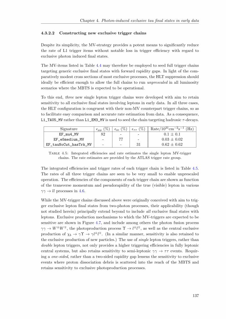
Chapter 4. Photon-induced exclusive tau final states in early data
4.3.2.2 Constructing new exclusive trigger chains
Despite its simplicity, the MV-strategy provides a potent means to significantly reduce
the rate of L1 trigger items without notable loss in trigger efficiency with regard to
exclusive photon induced final states.
The MV-items listed in Table 4.4 may therefore be employed to seed full trigger chains
targeting generic exclusive final states with forward rapidity gaps. In light of the com-
paratively modest cross sections of most exclusive processes, the HLT suppression should
ideally be efficient enough to allow the full chains to run unprescaled in all luminosity
scenarios where the MBTS is expected to be operational.
To this end, three new single lepton trigger chains were developed with aim to retain
sensitivity to all exclusive final states involving leptons in early data. In all three cases,
the HLT configuration is congruent with their non-MV counterpart trigger chains, so as
to facilitate easy comparison and accurate rate estimation from data. As a consequence,
L1_TAU5_MV rather than L1_EM3_MV is used to seed the chain targeting hadronic τ -decays.
Signature εµµ (%) εee (%) εττ (%) Rate/1031cm−2s−1 (Hz)
EF_mu4_MV 82 - - 0.1 ± 0.1EF_e5medium_MV - 77 - 0.03 ± 0.02
EF_tauNoCut_hasTrk_MV - - 31 0.62 ± 0.62
Table 4.5: Integrated efficiencies and rate estimates the single lepton MV-triggerchains. The rate estimates are provided by the ATLAS trigger rate group.
The integrated efficiencies and trigger rates of each trigger chain is listed in Table 4.5.
The rates of all three trigger chains are seen to be very small to enable unprescaled
operation. The efficiencies of the components of each trigger chain are shown as function
of the transverse momentum and pseudorapidity of the true (visible) lepton in various
γγ → ll processes in 4.6.
While the MV-trigger chains discussed above were originally conceived with aim to trig-
ger exclusive lepton final states from two-photon processes, their applicability (though
not studied herein) principally extend beyond to include all exclusive final states with
leptons. Exclusive production mechanisms to which the MV-triggers are expected to be
sensitive are shown in Figure 4.7, and include among others the photon fusion process
γγ → W±W∓, the photoproduction process Υ → l±l∓, as well as the central exclusive
production of χb → γΥ → γl±l∓. (In a similar manner, sensitivity is also retained to
the exclusive production of new particles.) The use of single lepton triggers, rather than
double lepton triggers, not only provides a higher triggering efficiencies in fully leptonic
central systems, but also retains sensitivity to semi-leptonic γγ → ττ events. Requir-
ing a one-sided, rather than a two-sided rapidity gap lessens the sensitivity to exclusive
events where proton dissociation debris is scattered into the reach of the MBTS and
retains sensitivity to exclusive photoproduction processes.
137
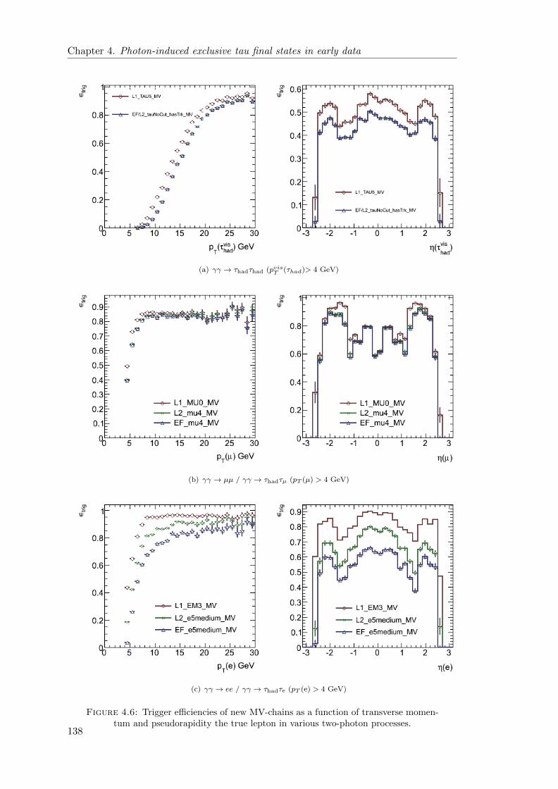
Chapter 4. Photon-induced exclusive tau final states in early data
(a) γγ → τhadτhad (pvisT (τhad)> 4 GeV)
(b) γγ → µµ / γγ → τhadτµ (pT (µ) > 4 GeV)
(c) γγ → ee / γγ → τhadτe (pT (e) > 4 GeV)
Figure 4.6: Trigger efficiencies of new MV-chains as a function of transverse momen-tum and pseudorapidity the true lepton in various two-photon processes.
138
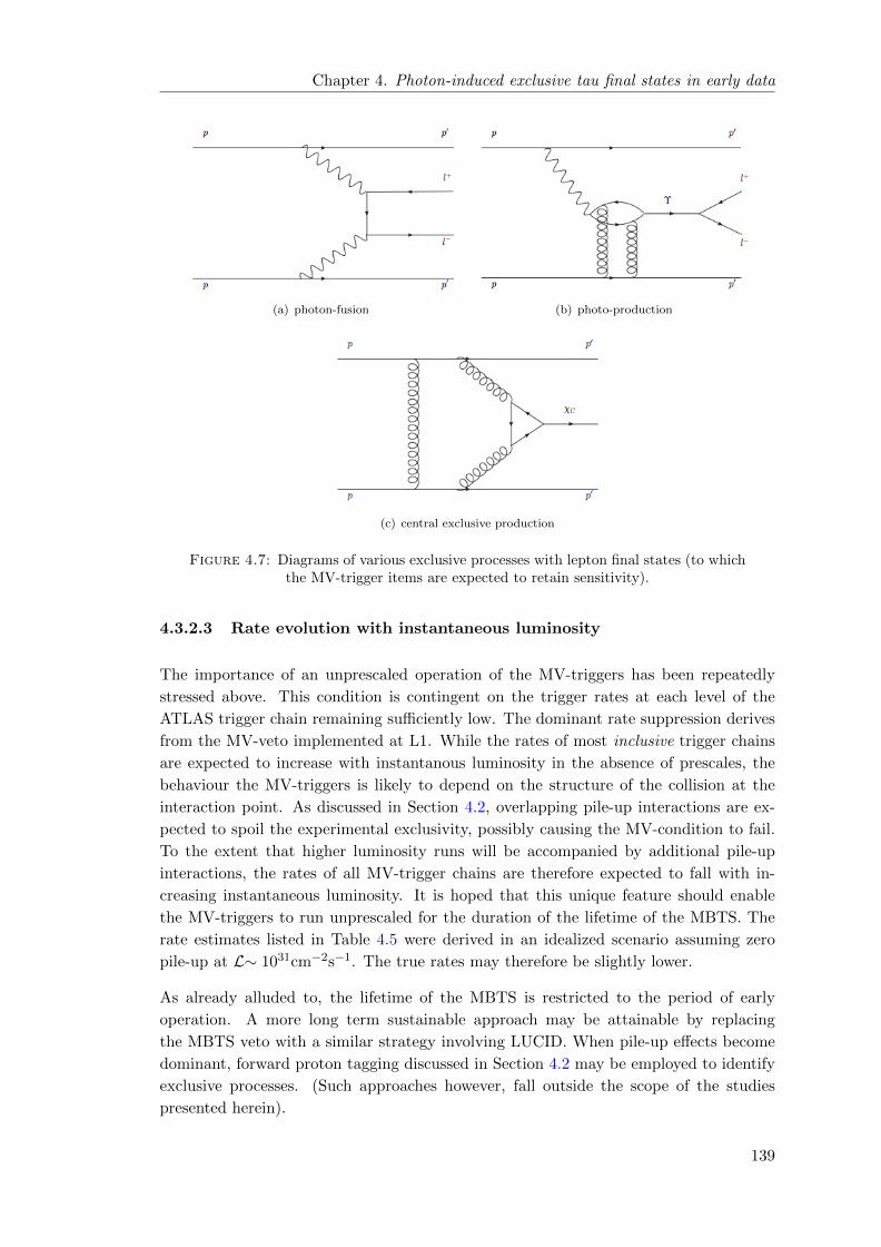
Chapter 4. Photon-induced exclusive tau final states in early data
(a) photon-fusion (b) photo-production
(c) central exclusive production
Figure 4.7: Diagrams of various exclusive processes with lepton final states (to whichthe MV-trigger items are expected to retain sensitivity).
4.3.2.3 Rate evolution with instantaneous luminosity
The importance of an unprescaled operation of the MV-triggers has been repeatedly
stressed above. This condition is contingent on the trigger rates at each level of the
ATLAS trigger chain remaining sufficiently low. The dominant rate suppression derives
from the MV-veto implemented at L1. While the rates of most inclusive trigger chains
are expected to increase with instantanous luminosity in the absence of prescales, the
behaviour the MV-triggers is likely to depend on the structure of the collision at the
interaction point. As discussed in Section 4.2, overlapping pile-up interactions are ex-
pected to spoil the experimental exclusivity, possibly causing the MV-condition to fail.
To the extent that higher luminosity runs will be accompanied by additional pile-up
interactions, the rates of all MV-trigger chains are therefore expected to fall with in-
creasing instantaneous luminosity. It is hoped that this unique feature should enable
the MV-triggers to run unprescaled for the duration of the lifetime of the MBTS. The
rate estimates listed in Table 4.5 were derived in an idealized scenario assuming zero
pile-up at L∼ 1031cm−2s−1. The true rates may therefore be slightly lower.
As already alluded to, the lifetime of the MBTS is restricted to the period of early
operation. A more long term sustainable approach may be attainable by replacing
the MBTS veto with a similar strategy involving LUCID. When pile-up effects become
dominant, forward proton tagging discussed in Section 4.2 may be employed to identify
exclusive processes. (Such approaches however, fall outside the scope of the studies
presented herein).
139
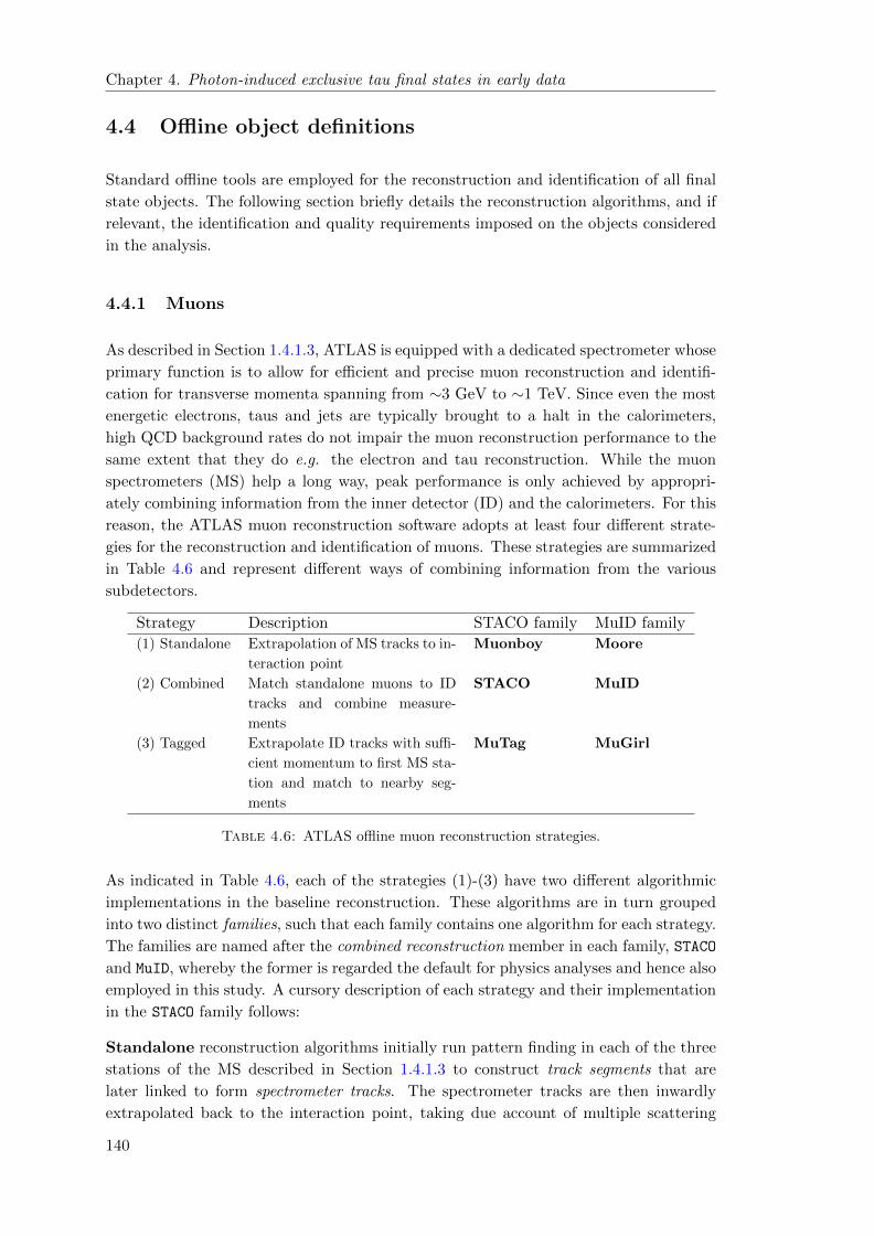
Chapter 4. Photon-induced exclusive tau final states in early data
4.4 Offline object definitions
Standard offline tools are employed for the reconstruction and identification of all final
state objects. The following section briefly details the reconstruction algorithms, and if
relevant, the identification and quality requirements imposed on the objects considered
in the analysis.
4.4.1 Muons
As described in Section 1.4.1.3, ATLAS is equipped with a dedicated spectrometer whose
primary function is to allow for efficient and precise muon reconstruction and identifi-
cation for transverse momenta spanning from ∼3 GeV to ∼1 TeV. Since even the most
energetic electrons, taus and jets are typically brought to a halt in the calorimeters,
high QCD background rates do not impair the muon reconstruction performance to the
same extent that they do e.g. the electron and tau reconstruction. While the muon
spectrometers (MS) help a long way, peak performance is only achieved by appropri-
ately combining information from the inner detector (ID) and the calorimeters. For this
reason, the ATLAS muon reconstruction software adopts at least four different strate-
gies for the reconstruction and identification of muons. These strategies are summarized
in Table 4.6 and represent different ways of combining information from the various
subdetectors.
Strategy Description STACO family MuID family
(1) Standalone Extrapolation of MS tracks to in-
teraction point
Muonboy Moore
(2) Combined Match standalone muons to ID
tracks and combine measure-
ments
STACO MuID
(3) Tagged Extrapolate ID tracks with suffi-
cient momentum to first MS sta-
tion and match to nearby seg-
ments
MuTag MuGirl
Table 4.6: ATLAS offline muon reconstruction strategies.
As indicated in Table 4.6, each of the strategies (1)-(3) have two different algorithmic
implementations in the baseline reconstruction. These algorithms are in turn grouped
into two distinct families, such that each family contains one algorithm for each strategy.
The families are named after the combined reconstruction member in each family, STACO
and MuID, whereby the former is regarded the default for physics analyses and hence also
employed in this study. A cursory description of each strategy and their implementation
in the STACO family follows:
Standalone reconstruction algorithms initially run pattern finding in each of the three
stations of the MS described in Section 1.4.1.3 to construct track segments that are
later linked to form spectrometer tracks. The spectrometer tracks are then inwardly
extrapolated back to the interaction point, taking due account of multiple scattering
140
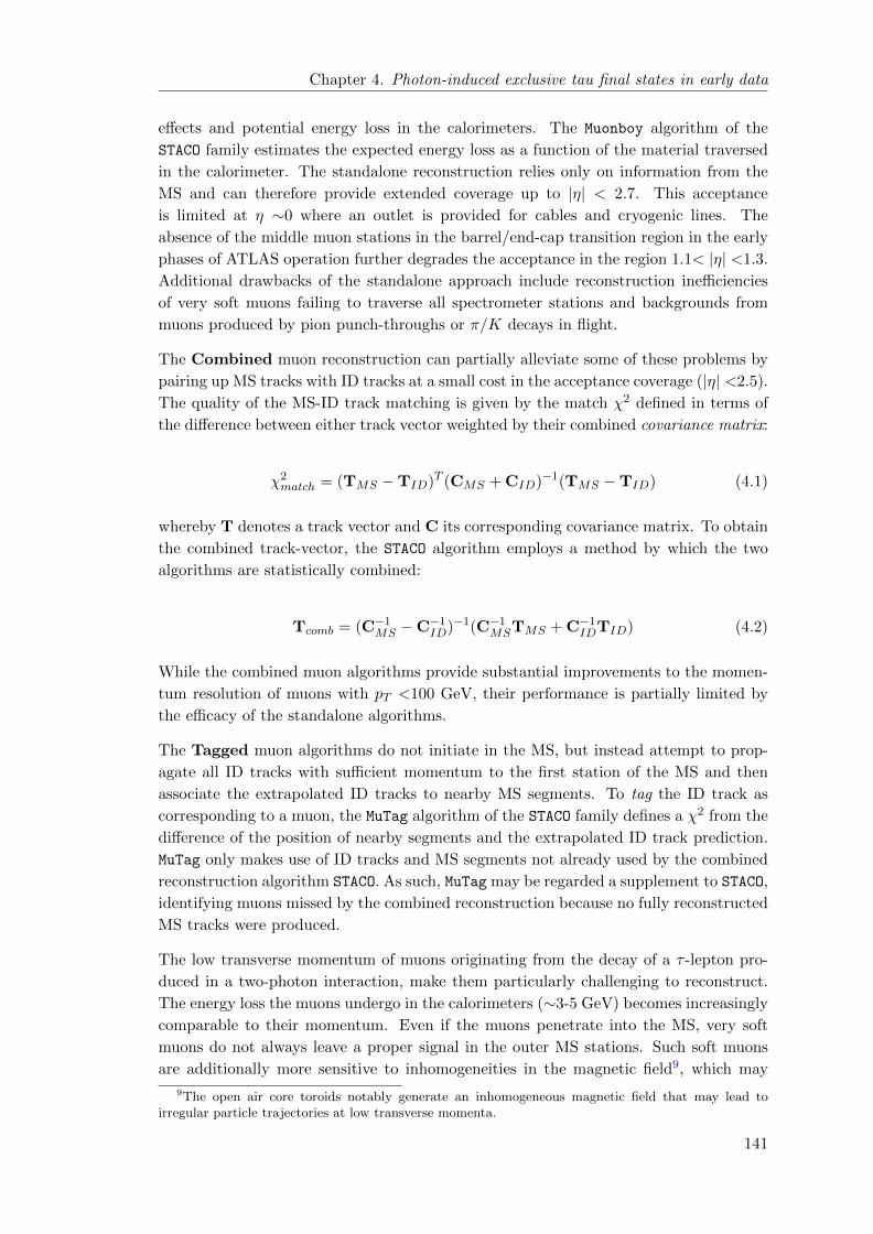
Chapter 4. Photon-induced exclusive tau final states in early data
effects and potential energy loss in the calorimeters. The Muonboy algorithm of the
STACO family estimates the expected energy loss as a function of the material traversed
in the calorimeter. The standalone reconstruction relies only on information from the
MS and can therefore provide extended coverage up to |η| < 2.7. This acceptance
is limited at η ∼0 where an outlet is provided for cables and cryogenic lines. The
absence of the middle muon stations in the barrel/end-cap transition region in the early
phases of ATLAS operation further degrades the acceptance in the region 1.1< |η| <1.3.
Additional drawbacks of the standalone approach include reconstruction inefficiencies
of very soft muons failing to traverse all spectrometer stations and backgrounds from
muons produced by pion punch-throughs or π/K decays in flight.
The Combined muon reconstruction can partially alleviate some of these problems by
pairing up MS tracks with ID tracks at a small cost in the acceptance coverage (|η| <2.5).
The quality of the MS-ID track matching is given by the match χ2 defined in terms of
the difference between either track vector weighted by their combined covariance matrix:
χ2match = (TMS −TID)T (CMS + CID)−1(TMS −TID) (4.1)
whereby T denotes a track vector and C its corresponding covariance matrix. To obtain
the combined track-vector, the STACO algorithm employs a method by which the two
algorithms are statistically combined:
Tcomb = (C−1MS −C−1
ID)−1(C−1MSTMS + C−1
IDTID) (4.2)
While the combined muon algorithms provide substantial improvements to the momen-
tum resolution of muons with pT <100 GeV, their performance is partially limited by
the efficacy of the standalone algorithms.
The Tagged muon algorithms do not initiate in the MS, but instead attempt to prop-
agate all ID tracks with sufficient momentum to the first station of the MS and then
associate the extrapolated ID tracks to nearby MS segments. To tag the ID track as
corresponding to a muon, the MuTag algorithm of the STACO family defines a χ2 from the
difference of the position of nearby segments and the extrapolated ID track prediction.
MuTag only makes use of ID tracks and MS segments not already used by the combined
reconstruction algorithm STACO. As such, MuTag may be regarded a supplement to STACO,
identifying muons missed by the combined reconstruction because no fully reconstructed
MS tracks were produced.
The low transverse momentum of muons originating from the decay of a τ -lepton pro-
duced in a two-photon interaction, make them particularly challenging to reconstruct.
The energy loss the muons undergo in the calorimeters (∼3-5 GeV) becomes increasingly
comparable to their momentum. Even if the muons penetrate into the MS, very soft
muons do not always leave a proper signal in the outer MS stations. Such soft muons
are additionally more sensitive to inhomogeneities in the magnetic field9, which may
9The open air core toroids notably generate an inhomogeneous magnetic field that may lead toirregular particle trajectories at low transverse momenta.
141

Chapter 4. Photon-induced exclusive tau final states in early data
(a) Muon reconstruction efficiency (b) Electron reconstruction efficiency
Figure 4.8: (a) Fractional reconstruction efficiency of muons reconstructed by STACO
(Combined) and MuTag (Tagged) as a function of the selected reconstructed muon trans-verse momentum in γγ → µµ and γγ → τhadτµ. The reconstructed muons are requiredto satisfy the selection outlined in Table 4.7. (b) Reconstruction efficiency with vari-ous cut-based identification methods vs reconstructed electron transverse momentum
in γγ → ee (pT >5 GeV)
result in complicated trajectories more difficult to reconstruct. Since MuTag does not
rely on reconstructed MS tracks, it targets and improves the reconstruction efficiency
in the very soft end of muon pT spectrum. Moreover, it is less sensitive to regions of
degraded performance in the MS.
Selection Description
Combined or Tagged Candidate is reconstructed by STACO or MuTag.χ2 < 100 Match quality requirement on combined muon candidatespT > 4 GeV Minimum transverse momentum requirement on muon candidatenucone40 < 5 Maximal number of tracks in an isolation cone of ∆R <0.4
Table 4.7: Muon preselection requirements.
The muon selection employed in this analysis is summarized in Table 4.7. Figure 4.8(a)
depicts the muon reconstruction efficiency of combined and tagged muons as a function
of the reconstructed muon transverse momentum in γγ → µµ and γγ → τhadτµ.
4.4.2 Electrons
The high rate of QCD jet production at the LHC puts stringent requirements on the
performance of electron identification tools in ATLAS. The ratio between the rates of
isolated electrons to that of QCD jets (20 < pjetT < 50 GeV) is expected to be ∼ 10−5,
a hundred times smaller than the corresponding ratio at the Tevatron [32]. In terms
of electron transverse momentum, the reconstruction requirements demanded by the
physics programme of ATLAS spans a broad kinematic range, from a few GeV to several
TeV. The challenge of reconstructing soft electrons, such as those originating from two-
photon processes, is exacerbated by the energy loss of electrons in the inner detector
volume. To meet with these challenges, complementary electron reconstruction routines
have been developed:
142
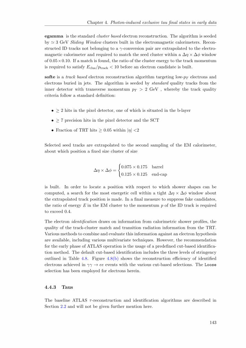
Chapter 4. Photon-induced exclusive tau final states in early data
egamma is the standard cluster based electron reconstruction. The algorithm is seeded
by ' 3 GeV Sliding Window clusters built in the electromagnetic calorimeters. Recon-
structed ID tracks not belonging to a γ-conversion pair are extrapolated to the electro-
magnetic calorimeter and required to match the seed cluster within a ∆η×∆φ window
of 0.05×0.10. If a match is found, the ratio of the cluster energy to the track momentum
is required to satisfy Eclus/ptrack < 10 before an electron candidate is built.
softe is a track based electron reconstruction algorithm targeting low-pT electrons and
electrons buried in jets. The algorithm is seeded by standard quality tracks from the
inner detector with transverse momentum pT > 2 GeV , whereby the track quality
criteria follow a standard definition:
• ≥ 2 hits in the pixel detector, one of which is situated in the b-layer
• ≥ 7 precision hits in the pixel detector and the SCT
• Fraction of TRT hits ≥ 0.05 within |η| <2
Selected seed tracks are extrapolated to the second sampling of the EM calorimeter,
about which position a fixed size cluster of size
∆η ×∆φ =
0.075× 0.175 barrel
0.125× 0.125 end-cap
is built. In order to locate a position with respect to which shower shapes can be
computed, a search for the most energetic cell within a tight ∆η × ∆φ window about
the extrapolated track position is made. In a final measure to suppress fake candidates,
the ratio of energy E in the EM cluster to the momentum p of the ID track is required
to exceed 0.4.
The electron identification draws on information from calorimetric shower profiles, the
quality of the track-cluster match and transition radiation information from the TRT.
Various methods to combine and evaluate this information against an electron hypothesis
are available, including various multivariate techniques. However, the recommendation
for the early phase of ATLAS operation is the usage of a predefined cut-based identifica-
tion method. The default cut-based identification includes the three levels of stringency
outlined in Table 4.8. Figure 4.8(b) shows the reconstruction efficiency of identified
electrons achieved in γγ → ee events with the various cut-based selections. The Loose
selection has been employed for electrons herein.
4.4.3 Taus
The baseline ATLAS τ -reconstruction and identification algorithms are described in
Section 2.2 and will not be given further mention here.
143
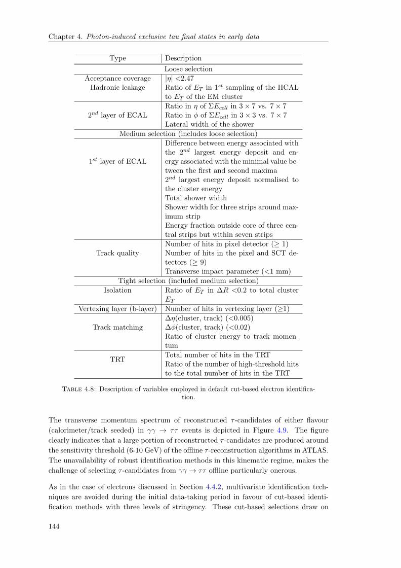
Chapter 4. Photon-induced exclusive tau final states in early data
Type Description
Loose selection
Acceptance coverage |η| <2.47Hadronic leakage Ratio of ET in 1st sampling of the HCAL
to ET of the EM cluster
2nd layer of ECALRatio in η of ΣEcell in 3× 7 vs. 7× 7Ratio in φ of ΣEcell in 3× 3 vs. 7× 7Lateral width of the shower
Medium selection (includes loose selection)
1st layer of ECAL
Difference between energy associated withthe 2nd largest energy deposit and en-ergy associated with the minimal value be-tween the first and second maxima2nd largest energy deposit normalised tothe cluster energyTotal shower widthShower width for three strips around max-imum stripEnergy fraction outside core of three cen-tral strips but within seven strips
Track qualityNumber of hits in pixel detector (≥ 1)Number of hits in the pixel and SCT de-tectors (≥ 9)Transverse impact parameter (<1 mm)
Tight selection (included medium selection)
Isolation Ratio of ET in ∆R <0.2 to total clusterET
Vertexing layer (b-layer) Number of hits in vertexing layer (≥1)
Track matching∆η(cluster, track) (<0.005)∆φ(cluster, track) (<0.02)Ratio of cluster energy to track momen-tum
TRTTotal number of hits in the TRTRatio of the number of high-threshold hitsto the total number of hits in the TRT
Table 4.8: Description of variables employed in default cut-based electron identifica-tion.
The transverse momentum spectrum of reconstructed τ -candidates of either flavour
(calorimeter/track seeded) in γγ → ττ events is depicted in Figure 4.9. The figure
clearly indicates that a large portion of reconstructed τ -candidates are produced around
the sensitivity threshold (6-10 GeV) of the offline τ -reconstruction algorithms in ATLAS.
The unavailability of robust identification methods in this kinematic regime, makes the
challenge of selecting τ -candidates from γγ → ττ offline particularly onerous.
As in the case of electrons discussed in Section 4.4.2, multivariate identification tech-
niques are avoided during the initial data-taking period in favour of cut-based identi-
fication methods with three levels of stringency. These cut-based selections draw on
144
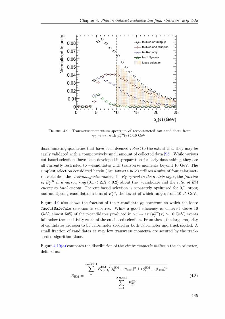
Chapter 4. Photon-induced exclusive tau final states in early data
Figure 4.9: Transverse momentum spectrum of reconstructed tau candidates fromγγ → ττ , with pgenT (τ) >10 GeV.
discriminating quantities that have been deemed robust to the extent that they may be
easily validated with a comparatively small amount of collected data [93]. While various
cut-based selections have been developed in preparation for early data taking, they are
all currently restricted to τ -candidates with transverse momenta beyond 10 GeV. The
simplest selection considered herein (TauCutSafeCalo) utilizes a suite of four calorimet-
ric variables: the electromagnetic radius, the ET spread in the η-strip layer, the fraction
of EEMT in a narrow ring (0.1 < ∆R < 0.2) about the τ -candidate and the ratio of EM
energy to total energy. The cut based selection is separately optimized for 0/1 prong
and multiprong candidates in bins of EvisT , the lowest of which ranges from 10-25 GeV.
Figure 4.9 also shows the fraction of the τ -candidate pT -spectrum to which the loose
TauCutSafeCalo selection is sensitive. While a good efficiency is achieved above 10
GeV, almost 50% of the τ -candidates produced in γγ → ττ (pgenT (τ) > 10 GeV) events
fall below the sensitivity reach of the cut-based selection. From these, the large majority
of candidates are seen to be calorimeter seeded or both calorimeter and track seeded. A
small fraction of candidates at very low transverse momenta are secured by the track-
seeded algorithm alone.
Figure 4.10(a) compares the distribution of the electromagnetic radius in the calorimeter,
defined as:
REM =
∆R<0.4∑i=1
EEMT,i
√(ηEMi − ηseed)2 + (φEM
i − φseed)2
∆R<0.4∑i=1
EEMT,i
(4.3)
145
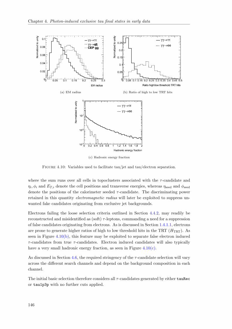
Chapter 4. Photon-induced exclusive tau final states in early data
(a) EM radius (b) Ratio of high to low TRT hits
(c) Hadronic energy fraction
Figure 4.10: Variables used to facilitate tau/jet and tau/electron separation.
where the sum runs over all cells in topoclusters associated with the τ -candidate and
ηi, φi and ET,i denote the cell positions and transverse energies, whereas ηseed and φseed
denote the positions of the calorimeter seeded τ -candidate. The discriminating power
retained in this quantity electromagnetic radius will later be exploited to suppress un-
wanted fake candidates originating from exclusive jet backgrounds.
Electrons failing the loose selection criteria outlined in Section 4.4.2, may readily be
reconstructed and misidentified as (soft) τ -leptons, commanding a need for a suppression
of false candidates originating from electrons. As is discussed in Section 1.4.1.1, electrons
are prone to generate higher ratios of high to low threshold hits in the TRT (HTRT). As
seen in Figure 4.10(b), this feature may be exploited to separate false electron induced
τ -candidates from true τ -candidates. Electron induced candidates will also typically
have a very small hadronic energy fraction, as seen in Figure 4.10(c).
As discussed in Section 4.6, the required stringency of the τ -candidate selection will vary
across the different search channels and depend on the background composition in each
channel.
The initial basic selection therefore considers all τ -candidates generated by either tauRec
or tau1p3p with no further cuts applied.
146
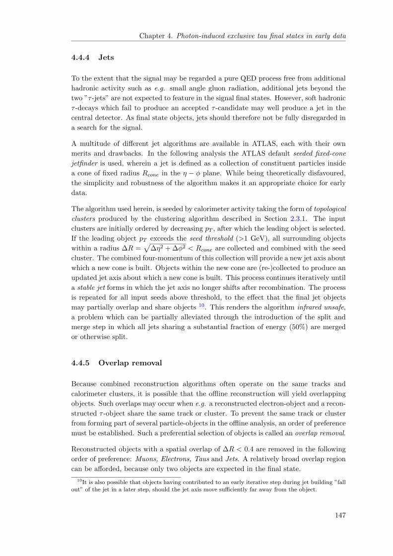
Chapter 4. Photon-induced exclusive tau final states in early data
4.4.4 Jets
To the extent that the signal may be regarded a pure QED process free from additional
hadronic activity such as e.g. small angle gluon radiation, additional jets beyond the
two ”τ -jets” are not expected to feature in the signal final states. However, soft hadronic
τ -decays which fail to produce an accepted τ -candidate may well produce a jet in the
central detector. As final state objects, jets should therefore not be fully disregarded in
a search for the signal.
A multitude of different jet algorithms are available in ATLAS, each with their own
merits and drawbacks. In the following analysis the ATLAS default seeded fixed-cone
jetfinder is used, wherein a jet is defined as a collection of constituent particles inside
a cone of fixed radius Rcone in the η − φ plane. While being theoretically disfavoured,
the simplicity and robustness of the algorithm makes it an appropriate choice for early
data.
The algorithm used herein, is seeded by calorimeter activity taking the form of topological
clusters produced by the clustering algorithm described in Section 2.3.1. The input
clusters are initially ordered by decreasing pT , after which the leading object is selected.
If the leading object pT exceeds the seed threshold (>1 GeV), all surrounding objects
within a radius ∆R =√
∆η2 + ∆φ2 < Rcone are collected and combined with the seed
cluster. The combined four-momentum of this collection will provide a new jet axis about
which a new cone is built. Objects within the new cone are (re-)collected to produce an
updated jet axis about which a new cone is built. This process continues iteratively until
a stable jet forms in which the jet axis no longer shifts after recombination. The process
is repeated for all input seeds above threshold, to the effect that the final jet objects
may partially overlap and share objects 10. This renders the algorithm infrared unsafe,
a problem which can be partially alleviated through the introduction of the split and
merge step in which all jets sharing a substantial fraction of energy (50%) are merged
or otherwise split.
4.4.5 Overlap removal
Because combined reconstruction algorithms often operate on the same tracks and
calorimeter clusters, it is possible that the offline reconstruction will yield overlapping
objects. Such overlaps may occur when e.g. a reconstructed electron-object and a recon-
structed τ -object share the same track or cluster. To prevent the same track or cluster
from forming part of several particle-objects in the offline analysis, an order of preference
must be established. Such a preferential selection of objects is called an overlap removal.
Reconstructed objects with a spatial overlap of ∆R < 0.4 are removed in the following
order of preference: Muons, Electrons, Taus and Jets. A relatively broad overlap region
can be afforded, because only two objects are expected in the final state.
10It is also possible that objects having contributed to an early iterative step during jet building ”fallout” of the jet in a later step, should the jet axis move sufficiently far away from the object.
147

Chapter 4. Photon-induced exclusive tau final states in early data
4.5 Backgrounds
An observation of the exclusive process γγ → ττ in early data relies on an efficient
elimination of all background processes that may falsely mimic the event signatures of
the signal process. The background processes may be classified as either non-exclusive or
exclusive. Each of these two categories present distinct challenges to the offline selection.
Each category also contains two classes of background processes, namely those containing
two τ -leptons in the final state and those whose final states contain < 2 τ -leptons but
other objects with a high likelihood of being falsely identified as τ -leptons.
4.5.1 Non-exclusive
Since the signal is characterised by a relatively balanced and central system accompanied
by large rapidity gaps void of detector activity to either side of the di-lepton axis, a
signal search criterium may be expressed as exclusively two τ -leptons and nothing else.
Non-exclusive backgrounds comprise all processes that also produce final states with two
central leptons, but always in company with something else. Most background processes
stemming from hard pp interactions may readily be identified as non-exclusive. This is
because the proton remnant in such scatters will typically leave signals in the forward
region of the central detector. Their reducibility hinges on a proper identification of any
additional activity between the leptons of the central system. While busier final states
typically enable such an identification, events from non-exclusive sources may still appear
exclusive if not all particles are properly accounted for, either because they are too soft
or because they escape into insensitive regions of the detector. While the occurrence of
such events is comparatively rare, the cross sections of most inclusive backgrounds are
typicallly many orders of magnitude larger than that of the exclusive signal. Efficient
suppression techniques are therefore called for.
A potential means of suppressing backgrounds from non-exclusive sources is by way of
calorimetric exclusivity:
Ωclus =
∑EclusT (|η| < 2.5)∑
EclusT
(4.4)
where the sum in the numerator runs over all topological clusters within |η| < 2.5 and
the sum in the denominator runs over all topological clusters in the event.
The distribution of Ωclus for the exclusive signal and various non-exclusive backgrounds
is shown in Figure 4.11(a). Calorimetric exclusivity as defined in Equation 4.4 is seen to
provide a highly efficient means to separate exclusive events from non-exclusive events.
This is particularly true for non-exclusive backgrounds where the energy scale of the
central objects is comparable to that expected from the signal. As the energy deposits in
the central calorimeters become large with respect to the forward deposits, the separation
power of Ωclus will naturally diminish. This effect is observed e.g. in the upper tail of
the Drell-Yan (DY) spectrum shown Figure 4.11(a).
148

Chapter 4. Photon-induced exclusive tau final states in early data
(a) (b)
Figure 4.11: (a) Calorimetric exclusivity in exclusive and non-exclusive processes.(b) Multiplicity of reconstructed objects after overlap removal in exclusive and non-
exclusive processes.
Event exclusivity may also be measured in terms of the multiplicity of reconstructed
objects. Figure 4.11(b) shows the sum of reconstructed tau, muon, electron and jet
objects after overlap removal. The number of reconstructed objects in the signal pro-
cess will rarely exceed two. This sets two-photon processes apart from non-exclusive
backgrounds, where additional activity beyond the hard scatter is likely to produce ad-
ditional objects in the event. Some degree of suppression may therefore be achieved by
removing events with an excess number of reconstructed objects. It is also noteworthy
that the soft nature of the signal will often generate final states void of reconstructed
objects, or final states with only one reconstructed object. An offline analysis requiring
two reconstructed objects will therefore be insensitive to a large portion of the signal.
Non-exclusive backgrounds considered herein, include:
• Minimum bias (non-diffractive)
• QCD dijets (8< pT <140 GeV)
• DY→ll (l=e,µ,τ)
• J/ψ →ll (l=e, µ)
• Υ→ µµ
Details pertaining to the Monte Carlo data samples are provided in Appendix B.3.
4.5.2 Exclusive backgrounds
Unlike non-exclusive backgrounds, exclusive backgrounds comprise all background pro-
cesses in which the rapidity gaps remain intact. Any features for differentiating the
exclusive signal from exclusive backgrounds must therefore be derived from the central
system alone. Exclusive backgrounds typically have much smaller cross sections than do
149
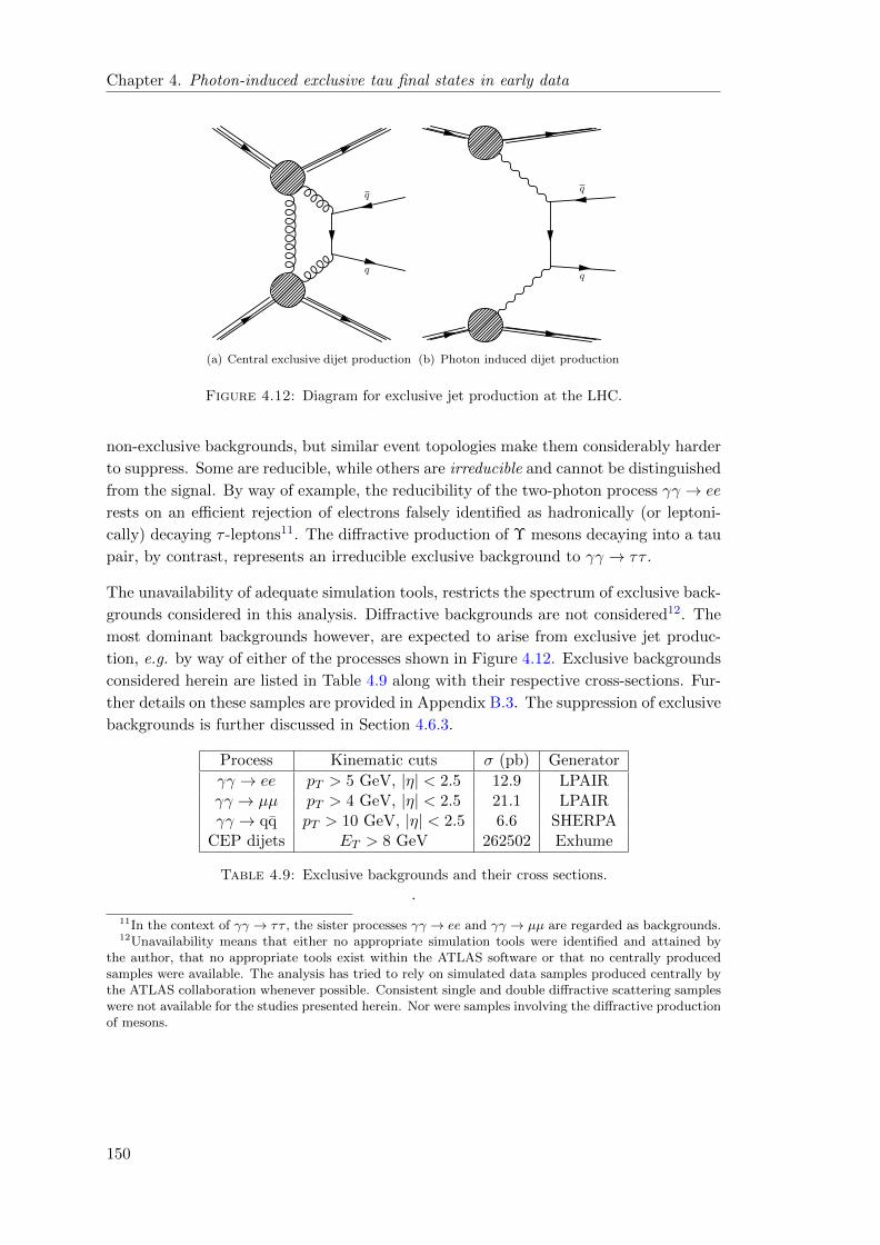
Chapter 4. Photon-induced exclusive tau final states in early data
q
q
(a) Central exclusive dijet production
q
q
(b) Photon induced dijet production
Figure 4.12: Diagram for exclusive jet production at the LHC.
non-exclusive backgrounds, but similar event topologies make them considerably harder
to suppress. Some are reducible, while others are irreducible and cannot be distinguished
from the signal. By way of example, the reducibility of the two-photon process γγ → ee
rests on an efficient rejection of electrons falsely identified as hadronically (or leptoni-
cally) decaying τ -leptons11. The diffractive production of Υ mesons decaying into a tau
pair, by contrast, represents an irreducible exclusive background to γγ → ττ .
The unavailability of adequate simulation tools, restricts the spectrum of exclusive back-
grounds considered in this analysis. Diffractive backgrounds are not considered12. The
most dominant backgrounds however, are expected to arise from exclusive jet produc-
tion, e.g. by way of either of the processes shown in Figure 4.12. Exclusive backgrounds
considered herein are listed in Table 4.9 along with their respective cross-sections. Fur-
ther details on these samples are provided in Appendix B.3. The suppression of exclusive
backgrounds is further discussed in Section 4.6.3.
Process Kinematic cuts σ (pb) Generator
γγ → ee pT > 5 GeV, |η| < 2.5 12.9 LPAIRγγ → µµ pT > 4 GeV, |η| < 2.5 21.1 LPAIRγγ → qq pT > 10 GeV, |η| < 2.5 6.6 SHERPA
CEP dijets ET > 8 GeV 262502 Exhume
Table 4.9: Exclusive backgrounds and their cross sections.
.
11In the context of γγ → ττ , the sister processes γγ → ee and γγ → µµ are regarded as backgrounds.12Unavailability means that either no appropriate simulation tools were identified and attained by
the author, that no appropriate tools exist within the ATLAS software or that no centrally producedsamples were available. The analysis has tried to rely on simulated data samples produced centrally bythe ATLAS collaboration whenever possible. Consistent single and double diffractive scattering sampleswere not available for the studies presented herein. Nor were samples involving the diffractive productionof mesons.
150

Chapter 4. Photon-induced exclusive tau final states in early data
4.5.3 Other background sources
In addition to inclusive and exclusive physics processes, various coincidence backgrounds
may mimic the exclusive signal in the detector. Such backgrounds may fake an exclusive
signature when several independent effects coincide.
Cosmic rays pass through ATLAS at random times. A cosmic event in the central
detector coinciding with a beam crossing involving e.g two single diffractive events or
one double diffractive event may well falsely appear as an exclusive signature.
By the same token, a cosmic event coinciding with an actual exclusive process may
destroy the exclusivity of the recorded event. Similarly, beam halo particles traversing
the long side of the detector may pollute the rapidity gaps of an exclusive event rendering
it effectively non-exclusive13.
Such effects are however expected to be small and will not be considered in the following.
4.6 Offline selection of the process γγ → ττ
In the following, an offline selection strategy is developed with aim to determine the
feasibility of extracting the process γγ → ττ from the first 100 pb−1 of√s = 7 TeV
data recorded by ATLAS assuming stable operation at an instantaneous luminosity
corresponding to L∼ 1031cm2s−1 and a beam configuration were pile-up effects are
negligible.
Differences in the experimental signatures associated with the signal and the various
background processes discussed in Section 4.5 provide the basic tools for a search for the
signal process in recorded data. The selection strategy attempts to target all possible
exclusive final states concurring with the following subsets of the signal:
• Fully hadronic channel: γγ → τhadτhad
• Semi-leptonic channel: γγ → τhadτµ and γγ → τhadτe
• Fully leptonic channel: γγ → τµτe
The offline selection itself may be regarded as a three-step procedure involving an initial
trigger selection, a secondary event preselection, followed by a more dedicated final
search into each target final state. The details pertaining to each step in the selection
procedure are given below.
13Beam Halo refers to secondary particles arising from elastic and inelastic beam proton scattersagainst residual gas inside the beam pipe.
151

Chapter 4. Photon-induced exclusive tau final states in early data
4.6.1 Online trigger selection
As was discussed in Section 4.3.2.2, dedicated trigger chains were developed in order to
retain online sensitivity to exclusive lepton final states during the period of early ATLAS
operation. The optimal trigger selection will necessarily depend on the exact configura-
tion of the trigger menu with which the recorded data is collected, and in particular on
the availability of low threshold trigger chains. Herein, the offline inspection will restrict
itself to events passing at least one of the following MV-trigger chains most of which
were detailed in Section 4.3.2.2:
• EF_tauNoCut_hasTrk_MV
• EF_j15_MV_MbSpTrk14
• EF_mu4_MV
• EF_e5medium_MV
under the assumption that all other low-pT trigger chains are rendered unsuitable by
large prescales.
Table 4.10 summarizes the efficiencies after trigger selection with respect to the signal
process and various exclusive and non-exclusive backgrounds.
While the trigger selection efficiency of the process γγ → ττ is limited, a large fraction
of γγ → ee and γγ → µµ events do pass the online trigger selection. While the explicit
offline selection of these processes will not be considered in the following study, these
processes are interesting in their own right. It is therefore notable that Table 4.10
indicates that sample sizes corresponding to approximately 1000 γγ → ee (pT (e) > 5
GeV) and 1800 γγ → µµ (pT (µ) > 4 GeV) are potentially made available for offline
analysis with an integrated luminosity of 100 pb−1.
The MBTS veto built into all the above trigger chains makes the trigger selection a
formidable suppressor of non-exclusive backgrounds. As a case in point, the trigger
selection efficiency of J/Ψ → ll is suppressed by O(103) with respect to γγ → ll.
Because inclusive background processes invariably involve radiation and proton debris
scattered into the pseudorapidity reach of the MBTS, they are highly unlikely to pass
the online selection.
4.6.2 Offline preselection
The offline event preselection seeks to reject all events whose global features do not
comply with the expected signatures of the signal. As discussed in Section 4.5, the signal
is most strikingly characterized by a small number of reconstructed particle objects and
minimal additional detector activity. Particle multiplicity and event exclusivity therefore
form the corner stone of the preselection:
14This trigger requires a 15 GeV jet, an MBTS-veto and at least one space-point track at L2.
152

Ch
apter
4.P
hoto
n-in
du
cedexclu
siveta
ufi
nal
states
inea
rlydata
Process Trigger Multiplicity Exclusivity Aεsel(%) N100 εsel(%) N100 εsel(%) N100
γγ → ττ (elastic) 38.16±0.22 30.9±0.2 37.00±0.22 30.0±0.2 36.32±0.22 29.4±0.2γγ → ττ (semi-elastic) 44.51±0.28 37.7±0.2 43.19±0.28 36.6±0.2 39.59±0.28 33.6±0.2γγ → ττ (inelastic) 50.20±0.24 51.9±0.2 48.70±0.23 50.4±0.3 41.02±0.23 42.4±0.2γγ → ee (elastic) 75.55±0.43 349.1±2.0 54.25±0.50 250.6±2.3 54.01±0.50 249.5±2.3γγ → ee (semi-elastic) 83.65±0.37 342.9±1.5 59.26±0.49 242.9±2.0 58.20±0.49 238.6±2.0γγ → ee (inelastic) 87.20±0.33 368.0±1.4 60.48±0.49 255.2±2.1 58.03±0.50 244.8±2.1γγ → µµ (elastic) 81.61±0.39 655.3±3.1 3.66 ±0.19 29.3±1.5 3.55±0.19 28.5±1.5γγ → µµ (semi-elastic) 87.86±0.32 572.8±2.1 4.37 ±0.21 28.4±1.4 4.19±0.20 27.3±1.3γγ → µµ (inelastic) 90.30±0.29 586.9±2.0 4.32 ±0.21 28.0±1.3 4.00 ±0.20 26.0±1.3
Minimum bias (ND) (2.48± 0.39) · 10−4 (12.0±1.86)·106 (2.09± 0.36) · 10−4 (10.0±1.7)·106 (1.10+1.02−0.62) · 10−5 533966+495440
−303428
QCD dijets 0.014±0.002 4.49·1010 ± 3.83 · 106 0.008±0.002 1.40·1010 ± 3.82 · 106 0.002±0.0008 1.03·109 ± 1.05 · 106
DY(ee/µµ/ττ) 0.33±0.01 4355±55 0.20±0.01 2709±43 0.015±0.002 209.2±7.6
J/Ψ\Υ 0.04±0.02 (103.11± 3.52) · 106 0.005±0.006 (15.4± 1.32)106 (2.08± 0.68) · 10−6 534747± 170766
Table 4.10: Selection efficiencies (εsel) and projective event numbers at 100 pb−1 (N100) of the trigger selection and event preselection.
153

Chapter 4. Photon-induced exclusive tau final states in early data
Figure 4.13: Fraction of events passing successive selection cuts for the signal and var-ious background processes. The efficiencies are measured with respect to the total eventsample in each process. Inclusive backgrounds are suppressed by O(∼ 105) through the
online and offline preselection, while exclusive backgrounds are largely unaffected.
4.6.2.1 Multiplicity
Depending on just how the di-tau system decays, the reconstructed final state is expected
to contain precisely two reconstructed τ -candidates or alternatively one τ -candidate ac-
companied by a reconstructed electron or muon. (To allow for the possibility that a
hadronically decaying τ -lepton does not produce a τ -candidate, but is instead recon-
structed as a jet, one single jet is permitted in the central detector (|η| < 2.5)). The
multiplicity preselection may then be summarized as follows:
1. At least one, but no more than two reconstructed leptons:
0 < Nleptons ≤ 2
2. No more than 1 light flavour lepton:
Ne ≤ 1 and Nµ ≤ 1
3. No additional jets:
Njets(|η| < 2.5) ≤ 1
where Nleptons signifies the sum of the number of selected electron object (Ne), muon
objects (Nµ) and tau candidate objects (Nτ ).
154
Chapter 4. Photon-induced exclusive tau final states in early data
4.6.2.2 Exclusivity A
The maximal number of tracks in the event should not exceed the six expected from
a fully hadronic double 3-prong decay. Moreover, significant energy deposits in the
calorimeter are only expected in the central detector. The exclusivity preselection may
therefore be summarized as:
1. Track multiplicity:
Ntracks ≤ 6
2. Calorimeter activity:
Ωclus > 0.9
Figure 4.13 compares the cummulative selection efficiency of the trigger and preselection
cuts in various processes.
In addition to reducing non-exclusive backgrounds with excess activity, the multiplicity
preselection is seen to diminish contamination from γγ → µµ. The exclusivity prese-
lection is seen to significantly suppress inclusive backgrounds passing the online trigger
selection.
4.6.3 Offline selectors
Events satisfying the event preselection are classified according to the particle content
in the event and passed to a generic selector which checks the kinematic balance of
the two-object system and checks for additional activity in between the pair of central
objects. Four categories were implemented in reflection of the final states expected from
the signal:
Selector A: targets the subprocess γγ → τhadτhad and is seeded by events con-
taining exclusively two τ -candidates.
Selector B: targets the subprocess γγ → τhadτµ and is seeded by events containing
exclusively one selected muon and one τ -candidate.
Selector C: targets the subprocess γγ → τhadτe and is seeded by events containing
one selected electron and one τ -candidate.
Selector D: targets the subprocess γγ → τµτe and is seeded by events containing
one selected muon and one selected electron.
The object pair in each selector A-D are required to satisfy the following kinematic
requirements:
|∆pT | ≤ 30 GeV and |∆φ| > 2.5
155

Chapter 4. Photon-induced exclusive tau final states in early data
Events satisfying the above kinematic constraints are further subjected to a second ex-
clusivity veto (”Exclusivity B”), whereby events with any detector activity at a distance
greater than ∆R >0.8 from both objects in a pair are rejected. Activity is defined in
terms of calorimeter clusters with Ecluster >5 GeV and tracks with ptrackT > 1.5 GeV.
The stringency on the τ -identification is tailored to the requirements imposed by the
distribution of backgrounds across the various selectors. The τ -object selection applied
in each selector are briefly summarized below.
Selector A
While the subprocess γγ → τhadτhad accounts for the largest portion of the visible cross
section for γγ → ττ , its offline selection is considerably challenged by background from
exclusive jet production. Moreover, soft electrons from γγ → ee failing the electron
selection may readily be misinterpreted as τ -candidates. Hence, comparatively vig-
orous methods for τ -identification and fake suppression are called for. Both selected
τ -candidates are therefore required to satisfy the TauCutSafeCaloLoose selection and
are further ”fortified” with the following selection criteria:
• Low track multiplicity: Ntrack = 0, 1 or 3
• Small EM radius: REM < 0.095
• Significant hadronic component: EEMEHAD
< 25
• Small ratio of high to low threshold TRT hits: HTRT < 0.12
A significant drop in the signal selection efficiency is expected to follow from the above
object selection requirements, principally caused by the transverse momentum cut built
into the TauCutSafeCaloLoose selection (pT > 10 GeV). As indicated in Figure 4.9,
most selected τ -candidates will have transverse momenta below this threshold.
Selector B
The presence of a muon significantly reduces backgrounds from exclusive jets and elec-
trons, permitting a more relaxed τ -object selection. The selected τ -candidate is therefore
only subjected to the following basic track requirement:
Ntracks = 1 or 3
To suppress fake candidates from γγ → µµ, the selected τ -candidate is further required
to pass the default muon veto in which track based τ -candidates with an energy com-
patible with a MIP muon are rejected.
Selector C
While the presence of an electron serves to suppress backgrounds from exclusive jets,
this search channel is very susceptible to background from γγ → ee where one electron
failing the electron selection described in Section 4.4.2 is available to generate a fake
τ -candidate.
156

Chapter 4. Photon-induced exclusive tau final states in early data
Selector NS NB Zn (30%) Zn (50%) Zn(100%)
A 3.9± 0.1 1.2+629.5−0.2 2.3 2.1 1.6
B 12.6± 0.2 1.2+629.5−0.2 5.5 5.1 4.2
C 3.5± 0.1 1.7+1.1−0.3 1.7 1.6 1.1
D 2.0± 0.1 0.04+0.1−0.03 3.1 3.1 2.9
Table 4.11: Expected number of signal (NS) and background (NB) events in selec-tors A-D with
∫L= 100pb−1 of data, along with associated significance Zn achieved
assuming 30%, 50% and 100% uncertainty on the background estimation.
To suppress backgrounds from γγ → ee, the selected τ -candidate is required to pass the
following selection:
• pT > 6 GeV and at least one associated track
• pass the tight electron veto if the candidate has an associated track seed
• significant hadronic energy fraction: EHADEEM+EHAD
> 0.1
• small ratio of high to low threshold TRT hits: HTRT < 0.12
Selector D
While this channel is almost void of backgrounds from both exclusive and inclusive
sources, it accounts for only ∼ 6% of the total signal cross section, making it particularly
challenging to select with modest integrated luminosities.
No further selection cuts of the muon and electron objects beyond those described in
Sections 4.4.1 and 4.4.2 are applied.
4.6.4 Results
The selection efficiencies of each selector described in Section 4.6.3 are summarized in
Tables 4.12-4.15. Backgrounds from which no selector seeds were generated have been
omitted. The errors are purely statistical and correspond to a 68.3 % confidence level
modelled on a binomial distribution [94]. The expected number of signal and background
events after all selection cuts are listed in Table 4.11. The table also lists the signal
significance Zn [56, 95]:
Zn =√
2Erf −1(1− 2p) (4.5)
where the p-value indicates the probability that the background fluctuates to ≥ n =
NS+NB. The p-value is here expressed in terms of a Poisson probability for a background
fluctuation to the observed signal, convoluted with a Gaussian background probability
density with mean value NB and standard deviation σNB encoding the uncertainty in
the background estimation:
157
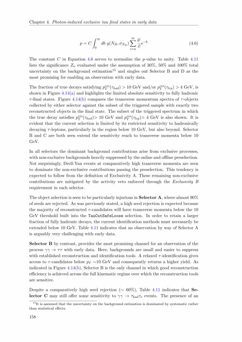
Chapter 4. Photon-induced exclusive tau final states in early data
p = C
∫ ∞0
db g(NB, σNB )
∞∑i=n
bi
i!e−b (4.6)
The constant C in Equation 4.6 serves to normalize the p-value to unity. Table 4.11
lists the significance Zn evaluated under the assumption of 30%, 50% and 100% total
uncertainty on the background estimation15 and singles out Selector B and D as the
most promising for enabling an observation with early data.
The fraction of true decays satisfying pvisT (τhad) > 10 GeV and/or pvisT (τlep) > 4 GeV, is
shown in Figure 4.14(a) and highlights the limited absolute sensitivity to fully hadronic
τ -final states. Figure 4.14(b) compares the transverse momentum spectra of τ -objects
collected by either selector against the subset of the triggered sample with exactly two
reconstructed objects in the final state. The subset of the triggered spectrum in which
the true decay satisfies pvisT (τhad)> 10 GeV and pvisT (τlep)> 4 GeV is also shown. It is
evident that the current selection is limited by its restricted sensitivity to hadronically
decaying τ -leptons, particularly in the region below 10 GeV, but also beyond. Selector
B and C are both seen extend the sensitivity reach to transverse momenta below 10
GeV.
In all selectors the dominant background contributions arise from exclusive processes,
with non-exclusive backgrounds heavily suppressed by the online and offline preselection.
Not surprisingly, Drell-Yan events at comparatively high transverse momenta are seen
to dominate the non-exclusive contributions passing the preselection. This tendency is
expected to follow from the definition of Exclusivity A. These remaining non-exclusive
contributions are mitigated by the activity veto enforced through the Exclusivity B
requirement in each selector.
The object selection is seen to be particularly injurious in Selector A, where almost 90%
of seeds are rejected. As was previously stated, a high seed rejection is expected because
the majority of reconstructed τ -candidates will have transverse momenta below the 10
GeV threshold built into the TauCutSafeLoose selection. In order to retain a larger
fraction of fully hadronic decays, the current identification methods must necessarily be
extended below 10 GeV. Table 4.11 indicates that an observation by way of Selector A
is arguably very challenging with early data.
Selector B by contrast, provides the most promising channel for an observation of the
process γγ → ττ with early data. Here, backgrounds are small and easier to suppress
with established reconstruction and identification tools. A relaxed τ -identification gives
access to τ -candidates below pT ∼10 GeV and consequently returns a higher yield. As
indicated in Figure 4.14(b), Selector B is the only channel in which good reconstruction
efficiency is achieved across the full kinematic regime over which the reconstruction tools
are sensitive.
Despite a comparatively high seed rejection (∼ 60%), Table 4.11 indicates that Se-
lector C may still offer some sensitivity to γγ → τhadτe events. The presence of an
15It is assumed that the uncertainty on the background estimation is dominated by systematic ratherthan statistical effects.
158

Chapter 4. Photon-induced exclusive tau final states in early data
(a) (b)
Figure 4.14: (a) The fraction of true decays satisfying pvisT (τhad) > 10 GeV and/orpvisT (τlep) > 4 GeV, selected by each offline selector after online trigger selection. (b)Transverse momentum spectrum of τ -candidates in the subset of the triggered signalwith exactly two reconstructed objects along with the subsets selected by Selectors A-C. The subsets corresponding to true pT (τhad) > 10 GeV and pT (τlep) > 4 GeV arealso shown for γγ → τhadτhad, γγ → τhadτµ and γγ → τhadτe decays. Selector B is seento be the only selector with a good efficiency with respect to the target process across
the full spectrum.
electron effectively suppresses backgrounds from exclusive jet production. The remain-
ing background therefore consists almost exclusively of poorly reconstructed events from
γγ → ee. As such, any observation in this channel will hinge on a robust and well un-
derstood electron veto.
Virtually background free, Selector D provides another promising channel for the ob-
servation of the process γγ → ττ through the fully leptonic channel. Despite the com-
paratively small branching fraction of the process γγ → τµτe, Table 4.11 indicates that
an observation may be possible in early data provided sufficient pile-up free data is at
hand.
About 30% of triggered signal events have only one reconstructed object in the final state.
Such events will automatically fail to qualify for any of the aforementioned selectors.
While it may be possible to recover some of these events by loosening the requirements
on the objects of the central system, (e.g. by seeding on a muon with back-to-back
activity in the form of a track system or calorimeter clusters), initial studies have proven
this a difficult task with only moderate gain.
The offline selection of fully leptonic same flavour decays, in which both τ -leptons decay
into either a pair of muons or a pair of electrons has not been attempted herein. While
such a selection is arguably very challenging in face of backgrounds from γγ → µµ and
γγ → ee, the distorted kinematics of the central system and small /ET caused by the
decay neutrinos may possibly offer a handle on the offline selection.
159

Ch
apte
r4.
Photo
n-i
ndu
ced
excl
usi
veta
ufi
nal
state
sin
earl
ydata
Process Seed Object selection Kinematics Exclusivity Bεsel(%) N100 εsel(%) N100 εsel(%) N100 εsel(%) N100
γγ → ττ (1.38± 0.01) · 10−1 37.3± 0.3 (1.75± 0.04) · 10−2 4.7± 0.1 (1.59± 0.04) · 10−2 4.2± 0.1 (1.46+0.04−0.03) · 10−2 3.9± 0.1
γγ → ee (1.41± 0.02)10−1 183± 3 (1.71+1.040.63 ) · 10−4 0.22+0.14
−0.08 (1.71+1.04−0.63) · 10−4 0.22+0.14
0.08 (1.71+1.040.63 ) · 10−4 0.22+0.14
0.08
γγ → qq (9.0± 0.3) · 10−2 60± 2 (1.80+0.46−0.39) · 10−3 1.2± 0.3 (1.80+0.46
−0.39) · 10−3 1.2± 0.3 (1.50+0.42−0.36) · 10−3 0.9+0.3
−0.2CEP gluons (1.1+0.2
−0.1) · 10−3 (2.89+0.41−0.37) · 104 < 2.30 · 10−5 < 603 < 2.30 · 10−5 < 603 < 2.30 · 10−5 < 603
Z→ee/ττ (5.71+0.40.3 ) · 10−5 9.7± 0.6 (1.40± 0.20) · 10−5 2.4± 0.3 (1.40± 0.20) · 10−5 2.4± 0.3 < 3.18 · 10−7 < 0.05
QCD dijets (2.93+0.48−0.44) 6437+1061
−956 (0.71+1.07−0.52) · 10−6 156+236
−115 (0.71+1.07−0.52) · 10−6 156+236
−115 < 8.22 · 10−7 < 180
Table 4.12: Selector A: tau-tau
Process Seed Object selection Kinematics Exclusivity Bεsel(%) N100 εsel(%) N100 εsel(%) N100 εsel(%) N100
γγ → ττ (5.51± 0.07) · 10−2 14.8± 0.2 (5.51± 0.07) · 10−2 14.8± 0.2 (4.94± 0.06) · 10−2 13.3± 0.2 (4.70± 0.06) · 10−4 12.6± 0.2γγ → µµ (8.16+1.86
1.47 ) · 10−4 1.7+0.4−0.3 (8.16+1.86
−1.47) · 10−4 1.7+0.4−0.3 (5.69+1.61
−1.22) · 10−4 1.1± 0.3 (5.69+1.611.22 ) · 10−4 1.1± 0.3
γγ → qq (1.47+0.43−0.36) · 10−3 0.9+0.3
−0.2 (3.16+2.26−1.52) · 10−4 0.2+0.2
−0.1 (3.16+2.26−1.52) · 10−4 0.2+0.2
−0.1 (3.16+2.26−1.52) · 10−4 0.2+0.2
−0.1CEP gluons (4.17+3.87
−2.37) · 10−4 1093+1015−621 < 2.39 · 10−5 < 628 < 2.39 · 10−5 < 628 < 2.39 · 10−5 < 628
Z → ττ (2.13+0.43−0.38) · 10−5 1.82+0.37
−0.32 (1.45+0.36−0.31) · 10−5 1.23+0.31
0.26 1.22+0.34−0.28 1.04+0.28
−0.24 < 8.77 · 10−7 0.07
Table 4.13: Selector B: tau-muon
Process Seed Object selection Kinematics Exclusivity Bεsel(%) N100 εsel(%) N100 εsel(%) N100 εsel(%) N100
γγ → ττ (4.37± 0.06)10−2 11.7± 0.2 (1.57± 0.04) · 10−2 4.2± 0.1 (1.41± 0.03) · 10−2 3.7± 0.1 (1.32± 0.03) · 10−2 3.5± 0.1γγ → ee (3.99± 0.03) · 10−1 518± 4 (1.4± 0.2) · 10−3 1.8± 0.3 (1.3± 0.2) · 10−3 1.7± 0.3 (1.2± 0.2) · 10−3 1.6± 0.3γγ → qq (1.1± 0.4) · 10−3 0.7± 0.2 (2+2
−1) · 10−4 0.13+0.12−0.08 (2+2
−1) · 10−4 0.13+0.12−0.08 (2+2
−1) · 10−4 0.13+0.12−0.08
DY (5.3+0.7−0.6) · 10−5 32± 4 (5.0+2.7
−1.7) · 10−6 3.0+1.61.0 (4.6+2.7
−1.7) 2.8+1.7−1.0 < 1.66 · 10−6 < 1.0
Table 4.14: Selector C: tau-electron
Process Seed Object selection Kinematics Exclusivity Bεsel(%) N100 εsel(%) N100 εsel(%) N100 εsel(%) N100
γγ → ττ (8.59+0.27−0.26) · 10−3 2.3± 0.1 (8.53+0.27
−0.26) · 10−3 2.2± 0.1 (7.78+0.26−0.25) · 10−3 2.0± 0.1 (7.54+0.25
−0.24) · 10−3 2.0± 0.1γγ → ee (3.33+7.40
2.44 ) · 10−5 0.04+0.10−0.03 (3.33+7.40
−2.44) · 10−5 0.04+0.10−0.03 (3.33+7.40
−2.44) · 10−5 0.04+0.10−0.03 (3.33+7.40
−2.44) · 10−5 0.04+0.10−0.03
Z → ττ (2.03+1.22−0.87) · 10−6 0.17± 0.01 (2.03+1.22
−0.87) · 10−6 0.17± 0.01 (2.03+1.22−0.87) · 10−6 0.17± 0.01 < 5.8410−7 < 0.05
Table 4.15: Selector D: muon-electron
160
Chapter 4. Photon-induced exclusive tau final states in early data
4.6.5 A note on systematic uncertainties
While the results summarized in Section 4.6.4 suggest that an observation of the pro-
cess γγ → ττ in early data collected by ATLAS may be possible, such an observation
hinges on a proper understanding and control of all possible effects that may introduce
systematic errors into the analysis. While a full consideration of systematic effects is
outside the scope of this analysis, a few potential sources of systematic uncertainties are
listed below.
The analysis is particularly vulnerable to any effects that might distort the exclusive
appearance of the signal. Even in the absence of additional pile-up interactions, such
distortions may arise from various machine backgrounds, as discussed in Section 4.5.3.
Moreover, the calorimetric exclusivity as enforced through the Exclusivity A and B selec-
tions in the offline analysis, is likely to be sensitive to the noise level in the calorimeters.
If noise fluctuations are large, an exclusive event may be mistakenly rejected as an in-
clusive events. Dead cells, while less likely to affect the signal selection efficiency, may
weaken the rejection of non-exclusive events 16. In a similar fashion, the online selection
will necessarily be sensitive to variations in the noise level and response pattern of the
MBTS.
The strong dependence of the cross section on the transverse momentum of the outgoing
central lepton pair, arguably makes the analysis sensitive to variations in both online
and offline object reconstruction efficiencies. Because the analysis presented herein uti-
lizes reconstruction tools close to their respective sensitivity thresholds, any degradation
in the reconstruction performance at low transverse momenta may severely impede a
successful observation.
4.7 Extending the reach with heavy ions
As was mentioned in Section 1.3.4, the LHC programme will include regular shorter
periods (∼1 month) of collision runs with heavy ions, during which the coherent action of
all the protons in a nucleus will serve to significantly enhance the production cross section
for two-photon processes. In recognition of this potential, studies have been undertaken
to explore the prospects offered by ultra-peripheral heavy ion collisions [96][97]. While
a study into the feasibility of utilizing such runs for the collection of γγ → ττ events
is outside the scope of this analysis, it is amusing to consider the prospects offered by
early heavy ion runs.
Table 4.16 lists cross sections as predicted by TPHIC MC [98]17 for the process γγ → ll
in Pb-Pb (Z=82) collisions at√sNN = 4/5.5 TeV/n.
The production cross sections are seen to increase significantly. Assuming early operation
with Pb-Pb collision at√sNN =4 TeV, Table 4.16 indicates that a few hundred γγ →
16Noisy cells may be identified and appropriately masked using data from collisions with empty events.Dead cells in the forward calorimeters should be identifiable with non-exclusive events.
17I am grateful to V. Pozdnyakov for providing the code.
161
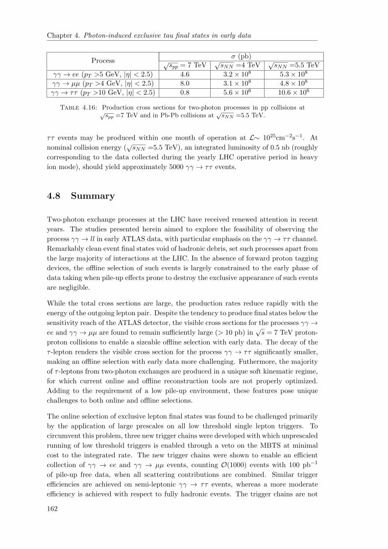
Chapter 4. Photon-induced exclusive tau final states in early data
Processσ (pb)√
spp = 7 TeV√sNN =4 TeV
√sNN =5.5 TeV
γγ → ee (pT >5 GeV, |η| < 2.5) 4.6 3.2× 10⁸ 5.3× 10⁸
γγ → µµ (pT >4 GeV, |η| < 2.5) 8.0 3.1× 10⁸ 4.8× 10⁸
γγ → ττ (pT >10 GeV, |η| < 2.5) 0.8 5.6× 10⁶ 10.6× 10⁶
Table 4.16: Production cross sections for two-photon processes in pp collisions at√spp =7 TeV and in Pb-Pb collisions at
√sNN =5.5 TeV.
ττ events may be produced within one month of operation at L∼ 1025cm−2s−1. At
nominal collision energy (√sNN =5.5 TeV), an integrated luminosity of 0.5 nb (roughly
corresponding to the data collected during the yearly LHC operative period in heavy
ion mode), should yield approximately 5000 γγ → ττ events.
4.8 Summary
Two-photon exchange processes at the LHC have received renewed attention in recent
years. The studies presented herein aimed to explore the feasibility of observing the
process γγ → ll in early ATLAS data, with particular emphasis on the γγ → ττ channel.
Remarkably clean event final states void of hadronic debris, set such processes apart from
the large majority of interactions at the LHC. In the absence of forward proton tagging
devices, the offline selection of such events is largely constrained to the early phase of
data taking when pile-up effects prone to destroy the exclusive appearance of such events
are negligible.
While the total cross sections are large, the production rates reduce rapidly with the
energy of the outgoing lepton pair. Despite the tendency to produce final states below the
sensitivity reach of the ATLAS detector, the visible cross sections for the processes γγ →ee and γγ → µµ are found to remain sufficiently large (> 10 pb) in
√s = 7 TeV proton-
proton collisions to enable a sizeable offline selection with early data. The decay of the
τ -lepton renders the visible cross section for the process γγ → ττ significantly smaller,
making an offline selection with early data more challenging. Futhermore, the majority
of τ -leptons from two-photon exchanges are produced in a unique soft kinematic regime,
for which current online and offline reconstruction tools are not properly optimized.
Adding to the requirement of a low pile-up environment, these features pose unique
challenges to both online and offline selections.
The online selection of exclusive lepton final states was found to be challenged primarily
by the application of large prescales on all low threshold single lepton triggers. To
circumvent this problem, three new trigger chains were developed with which unprescaled
running of low threshold triggers is enabled through a veto on the MBTS at minimal
cost to the integrated rate. The new trigger chains were shown to enable an efficient
collection of γγ → ee and γγ → µµ events, counting O(1000) events with 100 pb−1
of pile-up free data, when all scattering contributions are combined. Similar trigger
efficiencies are achieved on semi-leptonic γγ → ττ events, whereas a more moderate
efficiency is achieved with respect to fully hadronic events. The trigger chains are not
162

Chapter . Photon-induced exclusive tau final states in early data
restricted to γγ → ll, but should be sensitive to generic exclusive final states involving
leptons.
Finally, an offline selection strategy for the process γγ → ττ was presented targeting fully
hadronic, semi-leptonic and fully-leptonic final states. The offline selection is challenged
by large, but reducible non-exclusive backgrounds, various exclusive backgrounds and
inefficiencies of the reconstruction algorithms at low transverse momenta. An efficient
suppression of all large non-exclusive backgrounds is achieved. Suppression of remaining
exclusive backgrounds is best achieved in search channels targeting γγ → τhadτµ and
γγ → τµτe events, both in which an observation of the process γγ → ττ may be possible
with 100 pb−1 of pile-up free data. Such an observation would be the first observation
of the process γγ → ττ at a hadron collider facility.
163

Appendix A
The ATLAS coordinate system
and associated nomenclature
ATLAS employs a right-handed Cartesian coordinate system, whose origin is located at
the center of the detector and in which
the z-axis (horizontal) is directed along the beamline,
the x-axis (horizontal) points to the center of the LHC ring,
and the y-axis (vertical) points vertically upwards.
The associated polar coordinate system more commonly used herein is defined in terms
of:
The azimuthal angle φ ≡ arctanpypx
, φ ∈ [−π,+π], where φ = 0 corresponds to +x
and φ = π2 corresponds to +y.
The polar angle θ ≡ arctan pTpz
, θ ∈ [0, 2π], where θ = 0 corresponds to +z and
θ = π corresponds to -z
The polar angle is commonly parametrized in terms of the pseudorapidity η:
η = − ln
[tan
(θ
2
)]=
1
2ln
(|p|+ pz|p| − pz
)(A.1)
which approaches the true rapdidity y = 12 ln
(E+pzE−pz
)in the massless limit |p| ∼ E.
It is often convenient to parametrize the detector volume in terms of η and φ. The
direction of a particle can be expressed as a point in (η, φ)-space and the distance
between two locations (η1, φ1) and (η2, φ2) as ∆R ≡√
(η2 − η1)2 − (φ2 − φ1)2.
165

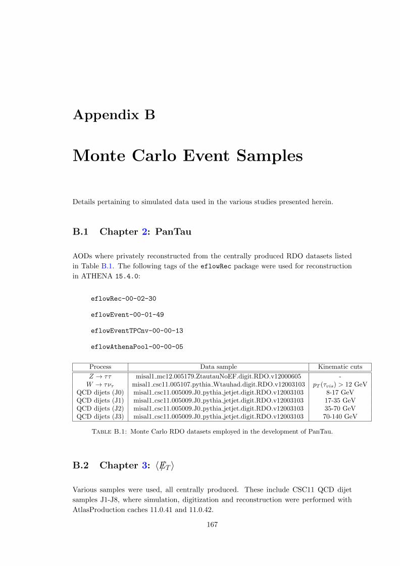
Appendix B
Monte Carlo Event Samples
Details pertaining to simulated data used in the various studies presented herein.
B.1 Chapter 2: PanTau
AODs where privately reconstructed from the centrally produced RDO datasets listed
in Table B.1. The following tags of the eflowRec package were used for reconstruction
in ATHENA 15.4.0:
eflowRec-00-02-30
eflowEvent-00-01-49
eflowEventTPCnv-00-00-13
eflowAthenaPool-00-00-05
Process Data sample Kinematic cuts
Z → ττ misal1 mc12.005179.ZtautauNoEF.digit.RDO.v12000605 -W → τντ misal1 csc11.005107.pythia Wtauhad.digit.RDO.v12003103 pT (τvis) > 12 GeV
QCD dijets (J0) misal1 csc11.005009.J0 pythia jetjet.digit.RDO.v12003103 8-17 GeVQCD dijets (J1) misal1 csc11.005009.J0 pythia jetjet.digit.RDO.v12003103 17-35 GeVQCD dijets (J2) misal1 csc11.005009.J0 pythia jetjet.digit.RDO.v12003103 35-70 GeVQCD dijets (J3) misal1 csc11.005009.J0 pythia jetjet.digit.RDO.v12003103 70-140 GeV
Table B.1: Monte Carlo RDO datasets employed in the development of PanTau.
B.2 Chapter 3: 〈 /ET 〉
Various samples were used, all centrally produced. These include CSC11 QCD dijet
samples J1-J8, where simulation, digitization and reconstruction were performed with
AtlasProduction caches 11.0.41 and 11.0.42.
167

Ap
pen
dix
B.
Mon
teC
arl
oE
ven
tS
am
ple
s
Data set Data sample pT -bin (GeV) Cross-section (mb) No. of events
trig1 misal1 csc11.005013.J4 pythia jetjet.recon.v12000605 005013 (J4) 140-280 3.077×10⁻⁴ 26.6ktrig1 misal1 csc11.005014.J5 pythia jetjet.recon.v12000605 005014 (J5) 280-560 1.258×10⁻⁵ 46.7ktrig1 misal1 csc11.005015.J6 pythia jetjet.recon.v12000605 005015 (J6) 560-1120 3.584×10⁻⁷ 33.0ktrig1 misal1 csc11.005016.J7 pythia jetjet.recon.v12000605 005016 (J7) 1120-2280 5.757×10⁻⁹ 0ktrig1 misal1 csc11.005017.J8 pythia jetjet.recon.v12000605 005017 (J8) > 2280 2.042×10⁻¹¹ 0k
trig1 misal1 mc12.008090.pythia J4 Nj2 FMET100.recon.v12000605 008090 (J4) 140-280 3.077×10⁻⁴ 5k/10ktrig1 misal1 mc12.008091.pythia J5 Nj2 FMET100.recon.v12000605 008091 (J5) 280-560 1.258×10⁻⁵ 33.3k/60ktrig1 misal1 mc12.008092.pythia J6 Nj2 FMET100.recon.v12000605 008092 (J6) 560-1120 3.584×10⁻⁷ 4k/20ktrig1 misal1 mc12.008093.pythia J7 Nj2 FMET100.merge.v12000605 008093 (J7) 1120-2280 5.757×10⁻⁹ 0k/5ktrig1 misal1 mc12.008094.pythia J8 Nj2 FMET100.merge.v12000605 008094 (J8) > 2280 2.042×10⁻¹¹ 0k/5k
Table B.2: Monte Carlo sample statistics.
168

Appendix B. Monte Carlo Event Samples
Validation studies of the generator filter mechanism with centrally produced unfiltered
and filtered samples were performed with the datasets listed in Table B.2. These samples
were passed through HighPtView-00-00-40 in ATHENA 12.0.6.
B.3 Chapter 4: γγ → ττ
B.3.1 Exclusive signal and exclusive backgrounds
All γγ → ll samples were privately generated with LPAIR [88, 89]. All γγ → qq samples
(q=u,d,s,c,b) were privately generated with SHERPA 1.2.1 [99] using the proton photon
PDFs:
(isr)
PDF_LIBRARY=MRST04QEDSherpa
PDF_SET=MRST04QED
PDF_GRID_PATH=MRST04Grid
(isr)
The output of either Monte Carlo generator was interfaced to ATHENA for full sim-
ulation, digitization and reconstruction. AtlasProduction cache 15.6.6.5 was used
throughout with:
• DB release: 9.6.1
• Conditions tag: OFLCOND-DR-BS7T-ANom-11
• Trigger configuration: MCRECO:DB:TRIGGERDBMC:107,61,92, corresponding to the
MC_lumi1E31_simpleL1Calib_physics_prescale trigger menu.
All other settings were concordant with the following production tags: s765 and r1250.
CEP gluon-gluon samples were centrally generated with Exhume [100] and privately re-
processed with the aforementioned simulation and reconstruction settings. All exclusive
samples used are listed in Table B.3.
B.3.2 Non-exclusive background processes
All non-exclusive background samples used were centrally produced and are listed in
Table B.4.
169
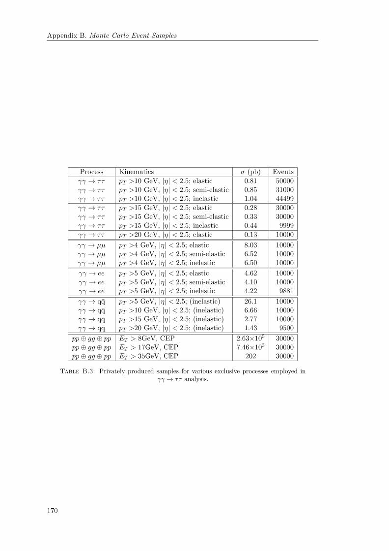
Appendix B. Monte Carlo Event Samples
Process Kinematics σ (pb) Events
γγ → ττ pT >10 GeV, |η| < 2.5; elastic 0.81 50000γγ → ττ pT >10 GeV, |η| < 2.5; semi-elastic 0.85 31000γγ → ττ pT >10 GeV, |η| < 2.5; inelastic 1.04 44499
γγ → ττ pT >15 GeV, |η| < 2.5; elastic 0.28 30000γγ → ττ pT >15 GeV, |η| < 2.5; semi-elastic 0.33 30000γγ → ττ pT >15 GeV, |η| < 2.5; inelastic 0.44 9999
γγ → ττ pT >20 GeV, |η| < 2.5; elastic 0.13 10000
γγ → µµ pT >4 GeV, |η| < 2.5; elastic 8.03 10000γγ → µµ pT >4 GeV, |η| < 2.5; semi-elastic 6.52 10000γγ → µµ pT >4 GeV, |η| < 2.5; inelastic 6.50 10000
γγ → ee pT >5 GeV, |η| < 2.5; elastic 4.62 10000γγ → ee pT >5 GeV, |η| < 2.5; semi-elastic 4.10 10000γγ → ee pT >5 GeV, |η| < 2.5; inelastic 4.22 9881
γγ → qq pT >5 GeV, |η| < 2.5; (inelastic) 26.1 10000γγ → qq pT >10 GeV, |η| < 2.5; (inelastic) 6.66 10000γγ → qq pT >15 GeV, |η| < 2.5; (inelastic) 2.77 10000γγ → qq pT >20 GeV, |η| < 2.5; (inelastic) 1.43 9500
pp⊕ gg ⊕ pp ET > 8GeV, CEP 2.63×10⁵ 30000pp⊕ gg ⊕ pp ET > 17GeV, CEP 7.46×10³ 30000pp⊕ gg ⊕ pp ET > 35GeV, CEP 202 30000
Table B.3: Privately produced samples for various exclusive processes employed inγγ → ττ analysis.
170

Ap
pen
dix
B.
Mon
teC
arlo
Even
tS
am
ples
Process σ (pb) Events ATLAS dataset (Prefix: mc09 7TeV., Suffix: r1260)
Minimum bias (ND) 484.45×10⁸ 1.81×10⁷ 105001.pythia_minbias.merge.AOD.e517_s787_s767_r1250
QCD (8-17 GeV) 985.34×10⁷ 1.10×10⁶ 105009.J0_pythia_jetjet.merge.AOD.e468_s766_s767_r1251
QCD (17-35 GeV) 678.03×10⁶ 1.08×10⁶ 105010.J1_pythia_jetjet.merge.AOD.e468_s766_s767_r1251
QCD (35-70 GeV) 409.79×10⁵ 1.40×10⁶ 105011.J2_pythia_jetjet.merge.AOD.e468_s766_s767_r1251
QCD (70-40 GeV) 219.60×10⁴ 1.40×10⁶ 105012.J3_pythia_jetjet.merge.AOD.e468_s766_s767_r1251
Z0/γ → e±e∓ 855.75 4.54×10⁶ 106046.PythiaZee_no_filter.merge.AOD.e468_s765_s767_r1250
Z0/γ → µ±µ∓ 855.64 4.43×10⁶ 106047.PythiaZmumu_no_filter.merge.AOD.e468_s765_s767_r1250
Z0/γ → τ±τ∓ 854.02 1.97×10⁶ 106052.PythiaZtautau.merge.AOD.e468_s765_s767_r1250
DY low M µ± (3 GeV) 4407 4.99×10⁵ 108321.PythiaDrellYanLowM_mu3.merge.AOD.e518_s765_s767_r1250
DY low M e± (3 GeV) 4406.1 4.99×10⁵ 108322.PythiaDrellYanLowM_ee3.merge.AOD.e518_s765_s767_r1250
DY low M τ± (Mττ >10 GeV) 3443.4 1.95×10⁵ 107055.PythiaDrellYanLowMtautau_M10.merge.AOD.e526_s765_s767_r1250
J/ψ → µ±µ∓ 2.31×10⁹ 4.97×10⁶ 108496.Pythia_directJpsimu0mu0.merge.AOD.e540_s765_s767_r1250
J/ψ → µ±µ∓ (4 GeV) 2.308×10⁹ 1.82×10⁶ 108407.Pythia_directJpsimu4mu4.merge.AOD.e477_s765_s767_r1250
J/ψ → e±e∓ (3 GeV) 246.58×10⁶ 8.99×10⁵ 105734.Pythia_direct_Jpsie3e3.merge.AOD.e511_s765_s767_r1250
Υ→ µ±µ∓ (4 GeV) 19.728×10⁶ 9.50×10⁴ 108484.Pythia_directUpsilonmu4mu4.merge.AOD.e477_s765_s767_r1250
Table B.4: Data samples for various inclusive processes employed in γγ → ττ analysis.
171


Appendix C
/EfakeT probability distribution
function
Derivation of the probability density distribution of N independent gaussian random
variables as a function of radial distance in the space defined by those variables.
Consider N independent gaussian random variables g(xi) of the general form:
g(xi) =1
σ√
2πexp
(x2i
2σ2
)where i ≤ N .
The probability P(R) of being in a small shell of volume dV at radius R is:
P(R) = g(x1, ..., xi, ..., xN )dV
=
N∏i=1
g(xi)dV
=1
σN (2π)N2
exp
(−r2
2σ2
)dV
= FN (r)dr
where FN (r) is the probability density of the this probability sphere as a function of
r =
√√√√ N∑i=1
x2i .
With the volume element dV is given as:
dV =πN2
Γ(N2 + 1
)NrN−1dr
173

Appendix C. /EfakeT probability distribution function
the probability density FN (r) can now be explicitly computed:
FN (r) =
[(√
2)N−2σNΓ
(N
2
)]−1
rN−1 exp
(−r2
2σ2
)
Finally, the mean value 〈r〉 of the probability density function FN (r) is given as:
〈r〉 =
∫rFN (r)dr
=
[(√
2)N−2σNΓ
(N
2
)]−1 ∫ ∞0
rN exp
(−r2
2σ2
)dr
=√
2σΓ(N+1
2
)Γ(N2
) .
174

Bibliography
[1] Lyndon Evans. The Large Hadron Collider: a marvel of technology. Fundamental
Sciences. EPFL Press, Lausanne, 2009.
[2] John Ellis and Keith A Olive. Supersymmetric Dark Matter Candidates. (CERN-
PH-TH-2010-004), Jan 2010. URL http://cdsweb.cern.ch/record/1234835?
ln=en.
[3] Christiane Lefevre. The CERN accelerator complex. Complexe des accelerateurs
du CERN. Jun 2006.
[4] Stefano Catani. Aspects of QCD, from the Tevatron to the LHC, 2000. URL
http://www.citebase.org/abstract?id=oai:arXiv.org:hep-ph/0005233.
[5] Bruning, Oliver Sim. LHC challenges and upgrade options. J. Phys.: Conf. Ser.,
110:112002, 2008.
[6] Rudiger Schmidt. The LHC accelerator: technology and first commis-
sioning. 430. WE-Heraeus-Seminar: Accelerators and Detectors at the
Technology Frontier, 2009. URL http://rudi.home.cern.ch/rudi/docs/
Hereaus-Bad-Honnef-2009.ppt.
[7] Bruning, Oliver Sim and Collier, Paul and Lebrun, P and Myers, Stephen and
Ostojic, Ranko and Poole, John and Proudlock, Paul. LHC Design Report. CERN,
Geneva, 2004. URL http://cdsweb.cern.ch/record/782076.
[8] Tevatron Run II Handbook, 2001. URL http://www-bd.fnal.gov/runII/.
[9] CERN Press Office. LHC to restart in 2009, 2008. URL http://press.web.cern.
ch/press/PressReleases/Releases2008/PR17.08E.html.
[10] CERN Press Office. LHC to run at 3.5 TeV for early part of 2009-2010 run
rising later, 2009. URL http://press.web.cern.ch/press/PressReleases/
Releases2009/PR13.09E.html.
[11] M. Giovannozzi W. Herr J. Jowett M. Lamont E. Shaposhnikova R. Assmann, M.
Ferro-Luzzi. Beam parameters and machine performance to be reached in 2010.
2010. URL http://lhc-commissioning.web.cern.ch/lhc-commissioning/
luminosity/MG_2010_parameters.pdf.
[12] Michelangelo L Mangano and T J Stelzer. Tools for the simulation of hard hadronic
collisions. Annu. Rev. Nucl. Part. Sci.
175

Bibliography
[13] F Petriello. Perturbative QCD for LHC Physics, 2009. URL http://www-conf.
slac.stanford.edu/ssi/2009/images/petriello080709.pdf.
[14] Michael E Peskin and Daniel V Schroeder. An Introduction to Quantum Field
Theory; 1995 ed. Westview, Boulder, CO, 1995.
[15] T. Ohl. Feynmanndiagramme fur Anfanger, 40. Herbstschule Maria Laach,
2.-12.09.08, 2008. URL http://maria-laach.physik.uni-siegen.de/Folien/
2008/Ohl/Laach2008.pdf.
[16] V. N. Gribov and L. N. Lipatov. Deep inelastic e p scattering in perturbation
theory. Sov. J. Nucl. Phys., 15:438–450, 1972.
[17] Guido Altarelli and G. Parisi. Asymptotic Freedom in Parton Language. Nucl.
Phys., B126:298, 1977.
[18] Yuri L. Dokshitzer. Calculation of the Structure Functions for Deep Inelastic
Scattering and e+ e- Annihilation by Perturbation Theory in Quantum Chromo-
dynamics. Sov. Phys. JETP, 46:641–653, 1977.
[19] John C. Collins, Davison E. Soper, and George Sterman. Factorization of Hard
Processes in QCD. Adv. Ser. Direct. High Energy Phys., 5:1–91, 1988. URL
http://aps.arxiv.org/abs/hep-ph/0409313v1.
[20] M. A. Dobbs et al. Les Houches guidebook to Monte Carlo generators for hadron
collider physics. 2004. URL http://arxiv.org/abs/hep-ph/0403045.
[21] B. R. Webber. Soft QCD and Monte Carlo, 2000. URL http://moriond.in2p3.
fr/QCD00/transparencies/4_wednesday/am/webber/proceedings.ps.gz.
[22] Bo Andersson, G. Gustafson, G. Ingelman, and T. Sjostrand. Parton Fragmenta-
tion and String Dynamics. Phys. Rept., 97:31–145, 1983.
[23] B. R. Webber. A QCD Model for Jet Fragmentation Including Soft Gluon Inter-
ference. Nucl. Phys., B238:492, 1984.
[24] The two-photon particle production mechanism. physical problems. applications.
equivalent photon approximation. Physics Reports, 15(4):181 – 282, 1975. ISSN
0370-1573.
[25] J. de Favereau de Jeneret et al. High energy photon interactions at the LHC. 2009.
URL http://arxiv.org/abs/0908.2020.
[26] Xavier Rouby. Measurements of photon induced processes in CMS and forward
proton detection at the LHC.
[27] K. Hencken et al. The Physics of Ultraperipheral Collisions at the LHC. Phys.
Rept., 458:1–171, 2008. URL http://arxiv.org/abs/hep-ex/0201034v1.
[28] G. Baur et al. Hot topics in ultra-peripheral ion collisions. 2002. URL http:
//arxiv.org/abs/hep-ex/0201034v1.
176

Bibliography Appendix C. /EfakeT probability distribution function
[29] M. G. Albrow et al. The FP420 R&D Project: Higgs and New Physics with
forward protons at the LHC. JINST, 4:T10001, 2009. URL http://arxiv.org/
pdf/0806.0302v2.
[30] F. Abe et al. (CDF Collaboration). Double parton scattering in pp collisions at√s = 1.8TeV . Phys. Rev. D, 56(7):3811–3832, Oct 1997.
[31] Mario Deile. Pileup Probabilities and Events per Bunch-Crossing. May 2007. URL
http://cdsweb.cern.ch/record/1109356/.
[32] G Aad. Expected performance of the ATLAS experiment: detector, trigger and
physics. CERN, Geneva, 2009. URL http://cdsweb.cern.ch/record/1125884.
[33] Predicted cross sections in mb from Phojet 1.12 and Pythia 6.420.
URL http://project-atlas-lucid.web.cern.ch/project-atlas-lucid/
taskforce/predicted_xs.pdf.
[34] David G. d’Enterria. Forward Physics at the LHC. 2007. URL http://arxiv.
org/abs/0708.0551.
[35] R. Kwee. Studies for the Development of a Minimum Bias Trigger at Low Lu-
minosities in the ATLAS-Experiment at the Large Hadron Collider, 2007. URL
http://www-atlas.desy.de/theses/Kwee_dipl.pdf.
[36] ATLAS: technical proposal for a general-purpose pp experiment at the Large
Hadron Collider at CERN. LHC Tech. Proposal. CERN, Geneva, 1994. URL
http://cdsweb.cern.ch/record/290968?ln=it.
[37] G. Aad et al. The ATLAS Experiment at the CERN Large Hadron Collider.
JINST, 3:S08003, 2008.
[38] Claude Amsler et al. Review of particle physics. Phys. Lett., B667:1, 2008.
[39] W. R. Leo. Techniques for Nuclear and Particle Physics Experiments. Springer,
1987.
[40] W H Bell, D Berge, J A Gray, R Kwee, B T Martin, A Messina, E L Nurse,
A J Richards, and P A Steinberg. MBTS trigger efficiency for the minimum
bias analysis using Inner Detector tracks from pp interactions at sqrt(s) = 900
GeV. Technical Report ATL-COM-DAQ-2010-003, CERN, Geneva, Jan 2010.
URL http://cdsweb.cern.ch/record/1235379/.
[41] Joleen Pater. The FP420 Project: The challenge of measuring forward protons at
the LHC. J. Phys. Conf. Ser., 110:092022, 2008. URL http://iopscience.iop.
org/1742-6596/110/9/092022/.
[42] S. Agostinelli et al. G4–a simulation toolkit. Nuclear Instruments and Methods
in Physics Research Section A: Accelerators, Spectrometers, Detectors and Associ-
ated Equipment, 506(3):250 – 303, 2003. URL http://www.sciencedirect.com/
science/article/B6TJM-48TJFY8-5/2/23ea98096ce11c1be446850c04cfa498.
177
Bibliography
[43] K Edmonds, S Fleischmann, T Lenz, C Magass, J Mechnich, and A Salzburger.
The Fast ATLAS Track Simulation (FATRAS). Technical Report ATL-SOFT-
PUB-2008-001. ATL-COM-SOFT-2008-002, CERN, Geneva, Mar 2008. URL
http://cdsweb.cern.ch/record/1091969.
[44] Michael Duehrssen and Karl Jakobs. Study of Higgs bosons in the WW final state
and development of a fast calorimeter simulation for the ATLAS experiment. PhD
thesis, Freiburg, University Freiburg, Freiburg, 2009. URL http://cdsweb.cern.
ch/record/1261372?ln=en.
[45] M. L. Perl, G. S. Abrams, A. M. Boyarski, M. Breidenbach, D. D. Briggs, F. Bu-
los, W. Chinowsky, J. T. Dakin, G. J. Feldman, C. E. Friedberg, D. Fryberger,
G. Goldhaber, G. Hanson, F. B. Heile, B. Jean-Marie, J. A. Kadyk, R. R. Larsen,
A. M. Litke, D. Luke, B. A. Lulu, V. Luth, D. Lyon, C. C. Morehouse, J. M.
Paterson, F. M. Pierre, T. P. Pun, and P. A. Rapidis. Evidence for anomalous
lepton production in e + −e− annihilation. Phys. Rev. Lett., 35(22):1489–1492,
Dec 1975. URL http://prl.aps.org/abstract/PRL/v35/i22/p1489_1.
[46] A. Pich. Tau physics. Adv. Ser. Direct. High Energy Phys., 15:453–492, 1998.
URL http://arxiv.org/abs/hep-ph/9704453.
[47] Bechtle et al. Identification of hadronic tau decays with ATLAS detector. Technical
Report ATL-PHYS-INT-2008-003. ATL-COM-PHYS-2007-066, CERN, Geneva,
Sep 2007. URL http://cdsweb.cern.ch/record/1059599?ln=en.
[48] C Limbach. Leptonische Tau-Zerfalle in supersymmetrischen Prozessen im
ATLAS-Detektor, 2009. URL http://lhc-ilc.physik.uni-bonn.de/thesis/
Diplomarbeit_climbach.pdf.
[49] Abdelhak Djouadi. The Anatomy of electro-weak symmetry breaking. II. The
Higgs bosons in the minimal supersymmetric model. Phys. Rept., 459:1–241, 2008.
URL http://arxiv.org/abs/hep-ph/0503172v2.
[50] Kaoru Hagiwara, (Ed. ), J. Kanzaki, (Ed. ), and N. Okada, (Ed. ). Supersymme-
try and unification of fundamental interactions. Proceedings, 12th International
Conference, SUSY 2004, Tsukuba, Japan, June 17-23, 2004. Prepared for 12th
International Conference on Supersymmetry and Unification of Fundamental In-
teractions (SUSY 04), Tsukuba, Japan, 17-23 Jun 2004.
[51] Ian Hinchliffe. Use of Taus in ATLAS. (hep-ph/0210340):6 p, Oct 2002. URL
http://cdsweb.cern.ch/record/588795/.
[52] C. Zendler. Studie zu supersymmetrischen Prozessen mit Taus im Endzustand im
ATLAS-Experiment am LHC, 2007. URL http://lhc-ilc.physik.uni-bonn.
de/thesis/Zendler.pdf.
[53] Till Nattermann, Klaus Desch, Peter Wienemann, and Carolin Zendler. Measuring
τ -polarisation in χ02 decays at the LHC. Journal of High Energy Physics, 2009(04):
057, 2009. URL http://stacks.iop.org/1126-6708/2009/i=04/a=057.
178

Bibliography Appendix C. /EfakeT probability distribution function
[54] Ketevi A Assamagan and Y Coadou. Determination of the charged Higgs mass
and of tan(beta) with ATLAS. Technical Report ATL-PHYS-2001-017, CERN,
Geneva, Nov 2001. URL http://cdsweb.cern.ch/record/685304?ln=en.
[55] A Christov, Y Coadou, Z Czyczula, M Janus, L Janyst, A Kaczmarska, A Kali-
nowski, J Komaragiri, S Lai, W Mader, N Meyer, E Richter-Was, Ch Ruwiedel,
and M Wolter. Performance of the tau reconstruction and identification algorithm
with release 14.2.20 and mc08 data. Technical Report ATL-COM-PHYS-2009-229,
CERN, Geneva, Apr 2009. URL http://cdsweb.cern.ch/record/1174957?ln=
en.
[56] G. Aad et al. Expected Performance of the ATLAS Experiment - Detector, Trigger
and Physics. 2009.
[57] Matteo Cacciari, Gavin P. Salam, and Gregory Soyez. The Anti-k(t) jet clustering
algorithm. JHEP, 0804:063, 2008. URL http://arxiv.org/abs/0802.1189.
[58] C. Schwanenberger. The Jet Calibration in the H1 Liquid Argon Calorimeter.
ArXiv Physics e-prints, September 2002. URL http://arxiv.org/abs/physics/
0209026.
[59] Buskulic et. al. Performance of the ALEPH detector at LEP. Nucl. Instrum.
Methods Phys. Res., A, 360(CERN-PPE-94-170. FSU-SCRI-95-70):481–506. 44 p,
Nov 1994. URL http://cdsweb.cern.ch/record/272484/?ln=it.
[60] M A Thomson. Particle Flow Calorimetry and the PandoraPFA Algorithm. Tech-
nical Report arXiv:0907.3577. CU-HEP-09-11, Jul 2009. URL http://cdsweb.
cern.ch/record/1192027/?ln=de.
[61] A. Bocci, S. Kuhlmann, S. Lami, G. Latino, and A. Bocci. Study of Jet Energy
Resolution at CDF. International Journal of Modern Physics A, 16:255–258, 2001.
URL http://adsabs.harvard.edu/abs/2001IJMPA..16S.255B.
[62] M C Hodgkinson, D R Tovey, and R Duxfield. Energy Flow Reconstruction with
the eflowRec Combined Reconstruction Software in Athena 15.6.9.8. Technical
report, CERN, Geneva. Note in preparation.
[63] Joanna Weng. A Global Event Description using Particle Flow with the CMS
Detector. Technical Report arXiv:0810.3686, Oct 2008. URL http://cdsweb.
cern.ch/record/1135775. Comments: Poster at ICHEP08, Philadelphia, USA,
July 2008. 3 pages.
[64] W Lampl, S Laplace, D Lelas, P Loch, H Ma, S Menke, S Rajagopalan,
D Rousseau, S Snyder, and G Unal. Calorimeter Clustering Algorithms: De-
scription and Performance. Technical Report ATL-LARG-PUB-2008-002. ATL-
COM-LARG-2008-003, CERN, Geneva, Apr 2008. URL http://cdsweb.cern.
ch/record/1099735/.
[65] J.-W. Tsung. Identification of 1-prong τ -decays into nπ0 Final States Using Topo-
logical Clusters with ATLAS, 2008. URL http://lhc-ilc.physik.uni-bonn.
de/thesis/Diplomarbeit_climbach.pdf.
179

Bibliography
[66] M C Hodgkinson, D R Tovey, and R Duxfield. Energy Flow Reconstruction with
eflowRec Combined Reconstruction Software in Athena 12.0.6. Technical Report
ATL-COM-PHYS-2007-082, CERN, Geneva, Oct 2007. URL https://cdsweb.
cern.ch/record-restricted/1064042/.
[67] T Barillari, E Bergeaas Kuutmann, T Carli, J Erdmann, P Giovannini, K J
Grahn, C Issever, A Jantsch, A Kiryunin, K Lohwasser, A Maslennikov, S Menke,
H Oberlack, G Pospelov, E Rauter, P Schacht, F Span, P Speckmayer, P Stavina,
and P Strzenec. Local Hadronic Calibration. Technical Report ATL-LARG-
PUB-2009-001. ATL-COM-LARG-2008-006, CERN, Geneva, Jun 2008. URL
http://cdsweb.cern.ch/record/1112035?ln=pl.
[68] Private communication with M. Hodgkinson.
[69] S Fleischmann, C Limbach, R Prabhu, and P Wienemann. PanTau: An energy-
flow based approach to τ -reconstruction in ATLAS. ATLAS note in preparation.
[70] Torbjorn Sjostrand, Stephen Mrenna, and Peter Z. Skands. PYTHIA 6.4 Physics
and Manual. JHEP, 05:026, 2006. URL http://arxiv.org/abs/hep-ph/
0603175v2.
[71] J Dingfelder, M Janus, and V Scharf. π0 Reconstruction in Tau Decays. Talk given
at the 2009 ATLAS Workshop on tau lepton physics (Copenhagen, Denmark).
[72] A Hcker, J Stelzer, F Tegenfeldt, H Voss, K Voss, A Christov, S Henrot-Versill,
M Jachowski, A Krasznahorkay, Y Mahalalel, X Prudent, and P Speckmayer.
TMVA - Toolkit for Multivariate Data Analysis with ROOT: Users guide. Tech-
nical Report CERN-OPEN-2007-007, CERN, Geneva, Mar 2007. URL http:
//tmva.sourceforge.net/docu/TMVAUsersGuide.pdf.
[73] S Fleischmann. Truth matching for reconstructed taus: Track-based matching
and ∆R matching. Talk given in ATLAS Tau Working Group Meeting, Jun
2009. URL http://indico.cern.ch/contributionDisplay.py?contribId=
5&confId=54879.
[74] Standard Definitions of Efficiency and Rejection for the Tau Working
Group. URL https://twiki.cern.ch/twiki/bin/view/AtlasProtected/
TauIdentification. ATLAS Tau Working Group internal TWIKI page.
[75] T Nattermann. Studie zu Effekten der Tau-Polarisation in den χ02-Zerfallen mit
dem ATLAS-Experiment, 2008. URL http://lhc-ilc.physik.uni-bonn.de/
thesis/DiplomarbeitNattermann.pdf.
[76] M Thomson. Particle Flow Calorimetry and ILC Detector Design. Seminar
talk given at Bonn University, Jan 2008. URL http://pi.physik.uni-bonn.
de/events.php?id=406.
[77] ATLAS computing: Technical Design Report. Technical Design Report ATLAS.
CERN, Geneva, 2005. URL http://cdsweb.cern.ch/record/837738. revised
version submitted on 2005-06-20 16:33:46.
180

Bibliography Appendix C. /EfakeT probability distribution function
[78] R Prabhu, K Desch, and P Wienemann. Estimating Missing Transverse Energy
at the Generator Level. Technical Report ATL-COM-PHYS-2007-019, CERN,
Geneva, Mar 2007. URL http://cdsweb.cern.ch/record/1024673/.
[79] ATLAS detector and physics performance: Technical Design Report, 2. Technical
Design Report ATLAS. CERN, Geneva, 1999. URL http://cdsweb.cern.ch/
record/391177.
[80] A. Abulencia et al. Observation of exclusive electron positron production in hadron
hadron collisions. Phys. Rev. Lett., 98:112001, 2007. doi: 10.1103/PhysRevLett.
98.112001. URL http://arxiv.org/abs/hep-ex/0611040v2.
[81] P. Achard et al. Muon pair and tau pair production in two-photon collisions at
LEP. Phys. Lett., B585:53–62, 2004. doi: 10.1016/j.physletb.2004.02.012.
[82] A. Aktas et al. Tau lepton production in e p collisions at HERA. Eur. Phys. J.,
C48:699–714, 2006. doi: 10.1140/epjc/s10052-006-0028-2.
[83] J. de Favereau de Jeneret et al. High energy photon interactions at the LHC. 2009.
[84] Valery A. Khoze, Alan D. Martin, R. Orava, and M. G. Ryskin. Luminosity mon-
itors at the LHC. Eur. Phys. J., C19:313–322, 2001. doi: 10.1007/s100520100616.
[85] Bryan Lawrence Caron. Luminosity measurement at the Large Hadron Collider.
UMI-NR-13944.
[86] V. I. Telnov A.G. Shamov. Precision luminosity measurement at LHC using two-
photon production of µ+µ− pairs. Nucl. Inst. & Meth., A 494:51–56, 2002.
[87] M Albrow and et al. Technical report.
[88] J. A. M. Vermaseren. Two Photon Processes at Very High-Energies. Nucl. Phys.,
B229:347, 1983. doi: 10.1016/0550-3213(83)90336-X.
[89] S. P. Baranov, O. Duenger, H. Shooshtari, and J. A. M. Vermaseren. LPAIR: A
generator for lepton pair production. In *Hamburg 1991, Proceedings, Physics
at HERA, vol. 3*1478-1482. (see HIGH ENERGY PHYSICS INDEX 30 (1992)
No.12988).
[90] F. et al Abe. Measurement of pp single diffraction dissociation at√s =546 and
1800 GeV. Phys. Rev. D, 50(9):5535–5549, Nov 1994. URL http://prd.aps.
org/abstract/PRD/v50/i9/p5535_1.
[91] 1031 Trigger Menu justification document for the old L1 calibration. AT-
LAS internal Twiki. URL https://twiki.cern.ch/twiki/bin/view/Atlas/
L31TriggerMenuOldL1Calib#Primary_egamma_triggers.
[92] Atlas Trigger Rates. URL https://twiki.cern.ch/twiki/bin/view/Atlas/
AtlasTriggerRates.
[93] Cut based identification of hadronic tau decays. Technical Report ATL-PHYS-
PUB-2010-001. ATL-COM-PHYS-2009-583, CERN, Geneva, Jan 2010. URL
http://cdsweb.cern.ch/record/1233743?ln=en.
181

Bibliography
[94] Marc Paterno. Calculating efficiencies and their uncertainties. 2003. URL http:
//home.fnal.gov/~paterno/images/effic.pdf. FERMILAB-TM-2286-CD.
[95] G Cowan. Discovery significance with statistical uncertainty in the background
estimate. URL http://www.pp.rhul.ac.uk/~cowan/stat/notes/SigCalcNote.
pdf.
[96] Ultraperipheral collisions with the ATLAS detector. Nuclear Physics B - Proceed-
ings Supplements, 184:180 – 181, 2008. ISSN 0920-5632. Proceedings of the Inter-
national Conference on the Structure and Interactions of the Photon, Including the
17th International Workshop on Photon-Photon Collisions and the International
Workshop on High Energy Photon Linear Colliders - PHOTON 2007.
[97] A Angerami, A Ajitanand, G Atoian, M D Baker, S Bathe, W K Brooks, P Chung,
B Cole, R Debbe, D Derendarz, J Dolejsi, N Grau, J Hill, W Holzmann, V Issakov,
J Jia, R Lacey, A Lebedev, M Leite, S Milov, P Nevski, A Olszewski, A Poblaguev,
V Pozdynakov, M Rosati, L Rosselet, M Rybar, H Santos, M Spousta, P Steinberg,
H Takai, S Timoshenko, A Trzupek, I Tserruya, F Videbaek, S White, B Wosiek,
K Wozniak, and M Zeller. Heavy Ion Physics with the ATLAS Detector at the
LHC. Technical Report ATL-COM-PHYS-2009-439, CERN, Geneva, Aug 2009.
URL http://cdsweb.cern.ch/record/1200454?ln=en.
[98] K. Hencken, Yu. V. Kharlov, G. V. Khaustov, S. A. Sadovsky, and V. D.
Samoylenko. TPHIC, event generator of two photon interactions in heavy ion
collisions. URL http://web.ihep.su/library/pubs/prep1996/96-38-e.htm.
IFVE-96-38.
[99] T. Gleisberg, S. Hche, F. Krauss, M. Schnherr, S. Schumann, F. Siegert, and
J. Winter. Event generation with SHERPA 1.1. Journal of High Energy Physics,
2009(02):007, 2009. URL http://stacks.iop.org/1126-6708/2009/i=02/a=
007.
[100] J. Monk and A. Pilkington. ExHuME: A Monte Carlo event generator for exclusive
diffraction. Comput. Phys. Commun., 175:232–239, 2006. URL http://arxiv.
org/abs/hep-ph/0502077.
182


![대신기계중량(지명원)-2013년.ppt [호환 모드] · DaeSin 서울양천구목3동613-2 정원오피스타운411호 (02)2649-8660, FAX: (02)2649-8663 E-mail : leemh3539@naver.com](https://img.dokumen.tips/doc/110x75/607fcc0d51bf4b058d101833/eoeeeee-2013eppt-eeoe-daesin-oeoeee3e613-2.jpg)