Embed Size (px)
Citation preview

University of Karlsruhe (TH)Interactive System LabsProf. Dr. Alexander Waibel
Studienarbeit
Informatik
Thema: Open-set Face Recognition
Lorant Szasz-Toth - [email protected]
JANUAR 2008
Betreuer: Prof. Dr. Alexander WaibelDr.-Ing. Rainer StiefelhagenHazım K. Ekenel

Abstract
This work presents a local appearance-based approach to open-set face recognition. Theopen-set recognition task is formulated as a multi-verification problem. The recognitiontask is carried out as a series of verifications, every new probes’ identity is establishedby performing identity verifications against each known subject in the gallery. Theclassification is based on local appearance-based face recognition approach using DCT.Input images are divided into local blocks to which the discrete cosine transform isapplied. A feature vector is then generated by combining selected local feature coeffi-cients and classification is performed using either support vector machines or nearestneighbor method. Progressive accumulation of confidence scores from each verifier isused to enhance video-based identification. Additionally, a data set has been collectedin front of the entry to an office to evaluate the performance of the proposed approach.

Open-set Face Recognition I
Contents
1 Introduction 1
1.1 Previous work . . . . . . . . . . . . . . . . . . . . . . . . . . . . . . . . 2
1.1.1 Holistic approaches . . . . . . . . . . . . . . . . . . . . . . . . . 3
1.1.2 Local appearance-based approaches . . . . . . . . . . . . . . . . 4
1.1.3 Face verification . . . . . . . . . . . . . . . . . . . . . . . . . . . 4
1.1.4 Open-set face recognition . . . . . . . . . . . . . . . . . . . . . . 5
2 Methodology 6
2.1 Haar cascade classifiers . . . . . . . . . . . . . . . . . . . . . . . . . . . 6
2.1.1 Haar-like features . . . . . . . . . . . . . . . . . . . . . . . . . . 6
2.1.2 Integral image . . . . . . . . . . . . . . . . . . . . . . . . . . . . 7
2.1.3 Boosted classifier cascades . . . . . . . . . . . . . . . . . . . . . 8
2.2 Discrete cosine transformation . . . . . . . . . . . . . . . . . . . . . . . 9
2.3 Local appearance-based face recognition using DCT . . . . . . . . . . . 10
2.4 Support vector machines . . . . . . . . . . . . . . . . . . . . . . . . . . 11
2.4.1 Linear classification . . . . . . . . . . . . . . . . . . . . . . . . . 11
2.4.2 Soft-margin linear classification . . . . . . . . . . . . . . . . . . 12
2.4.3 Non-linear classification . . . . . . . . . . . . . . . . . . . . . . 13
2.5 Nearest neighbor classification . . . . . . . . . . . . . . . . . . . . . . . 13
2.6 K-Means clustering . . . . . . . . . . . . . . . . . . . . . . . . . . . . . 14
3 Open-Set Face Recognition 16
3.1 Face registration . . . . . . . . . . . . . . . . . . . . . . . . . . . . . . 16
3.1.1 Face detection . . . . . . . . . . . . . . . . . . . . . . . . . . . . 16
3.1.2 Eye detection . . . . . . . . . . . . . . . . . . . . . . . . . . . . 16
3.1.3 Alignment . . . . . . . . . . . . . . . . . . . . . . . . . . . . . . 17
3.1.4 Sample augmentation . . . . . . . . . . . . . . . . . . . . . . . . 17
3.2 Feature extraction . . . . . . . . . . . . . . . . . . . . . . . . . . . . . 19
3.2.1 Local DCT coefficients . . . . . . . . . . . . . . . . . . . . . . . 19
3.2.2 Feature normalization . . . . . . . . . . . . . . . . . . . . . . . 19
3.3 Classification . . . . . . . . . . . . . . . . . . . . . . . . . . . . . . . . 20
3.3.1 SVM based classification . . . . . . . . . . . . . . . . . . . . . . 21
3.3.2 Nearest-neighbor based classification . . . . . . . . . . . . . . . 22
3.4 Video information incorporation . . . . . . . . . . . . . . . . . . . . . . 22
3.4.1 Temporal fusion with progressive scores . . . . . . . . . . . . . . 23
4 Experiments 24

II Open-set Face Recognition
4.1 Experimental setup . . . . . . . . . . . . . . . . . . . . . . . . . . . . . 24
4.2 Data set . . . . . . . . . . . . . . . . . . . . . . . . . . . . . . . . . . . 24
4.3 Open-set face recognition performance . . . . . . . . . . . . . . . . . . 27
4.3.1 Comparison of baseline SVM-based and NN-based open-set facerecognition . . . . . . . . . . . . . . . . . . . . . . . . . . . . . 27
4.3.2 Performance comparison . . . . . . . . . . . . . . . . . . . . . . 27
4.4 Further experiments . . . . . . . . . . . . . . . . . . . . . . . . . . . . 30
4.4.1 Influence of the number of training sessions . . . . . . . . . . . 30
4.4.2 Influence of the number of subjects . . . . . . . . . . . . . . . . 30
4.4.3 Influence of time span between training and testing . . . . . . . 32
4.4.4 Influence of undersampling . . . . . . . . . . . . . . . . . . . . . 34
4.5 Classification performance optimization . . . . . . . . . . . . . . . . . . 34
4.5.1 Improvement of video-based classification . . . . . . . . . . . . . 34
4.5.2 Sample augmentation . . . . . . . . . . . . . . . . . . . . . . . . 37
4.6 Overall system performance . . . . . . . . . . . . . . . . . . . . . . . . 38
4.7 System runtime performance . . . . . . . . . . . . . . . . . . . . . . . . 39
5 Conclusion 40

Open-set Face Recognition III
List of Figures
1 Different face recognition tasks . . . . . . . . . . . . . . . . . . . . . . 3
2 Sample Haar-like features . . . . . . . . . . . . . . . . . . . . . . . . . 6
3 Integral image representation . . . . . . . . . . . . . . . . . . . . . . . 7
4 Haar classifier cascades. . . . . . . . . . . . . . . . . . . . . . . . . . . 9
5 DCT image bases . . . . . . . . . . . . . . . . . . . . . . . . . . . . . . 10
6 Maximum margin classification . . . . . . . . . . . . . . . . . . . . . . 11
7 Non-linear classification using kernel functions . . . . . . . . . . . . . . 13
8 Face and eye detection . . . . . . . . . . . . . . . . . . . . . . . . . . . 18
9 Face with failed eye detection . . . . . . . . . . . . . . . . . . . . . . . 18
10 Zig-zag-scan of coefficients . . . . . . . . . . . . . . . . . . . . . . . . . 20
11 Images from dataset . . . . . . . . . . . . . . . . . . . . . . . . . . . . 26
12 Receiver Operating Characteristics curves . . . . . . . . . . . . . . . . 29
13 Development of classification scores with number of training sessions . . 31
14 Development of classification scores with number of subjects . . . . . . 33
15 Development of scores . . . . . . . . . . . . . . . . . . . . . . . . . . . 35
16 Classification score by frame . . . . . . . . . . . . . . . . . . . . . . . . 36

IV Open-set Face Recognition
List of Tables
1 SVM parameters . . . . . . . . . . . . . . . . . . . . . . . . . . . . . . 24
2 The data set . . . . . . . . . . . . . . . . . . . . . . . . . . . . . . . . . 26
3 Data set for open-set performance experiments . . . . . . . . . . . . . . 28
4 Nearest-neighbor classification results . . . . . . . . . . . . . . . . . . . 28
5 SVM classification results, with parametrized hyperplane ∆ = −0.12 . . 28
6 Influence of the number of training sessions . . . . . . . . . . . . . . . . 30
7 Data set for testing the influence of the number of subject . . . . . . . 31
8 Number of examined combinations . . . . . . . . . . . . . . . . . . . . 32
9 Influence of the number of training sessions . . . . . . . . . . . . . . . . 32
10 Influence of time span between training and testing . . . . . . . . . . . 33
11 Effect of undersampling . . . . . . . . . . . . . . . . . . . . . . . . . . 34
12 Reduced data set . . . . . . . . . . . . . . . . . . . . . . . . . . . . . . 35
13 SVM classification results . . . . . . . . . . . . . . . . . . . . . . . . . 36
14 Nearest-neighbor classification results . . . . . . . . . . . . . . . . . . . 36
15 Influence of sample augmentation with two known training sessions . . 38
16 Influence of sample augmentation with four known training sessions . . 38
17 Improvement of classification results by increasing the neighborhoodwhich is used to generate augmentated samples . . . . . . . . . . . . . 38
18 Overall system performance using sample augmentation, SVM-basedclassification, progressive score-based classification . . . . . . . . . . . . 39
19 System runtime performance . . . . . . . . . . . . . . . . . . . . . . . . 39

Open-set Face Recognition 1
1 Introduction
Face recognition plays an important role in human-machine interaction. Especiallysmart environments need robust and unobtrusive means of identifying interaction part-ners in order to achieve the goal of assisting the user without interference.
Face recognition is a natural and innate ability of humans and is used daily by every-body. Usually, we visually identify our communication partner. This further influencesour behavior and helps to improve interaction. Once the identity has been established,it is possible to tap background knowledge in order to better interpret intentions,statements and gestures or modify the own behavior.
Allowing a system to identify its interaction partners helps it to adapt to the user. Asample application domain is customized services based on the user’s preferences. Forexample, a car can recognize its driver and adjust cockpit and seat settings to the user’staste or a smart living room that adjusts ambient lighting and favorite TV channels.
This work focuses on an open-set face recognition scenario. Open-set recognition is thetask of identifying a set of known people from an open set of possible probes, closed-setrecognition on the other hand assumes that every probe is from a closed set of subjectsthat the system was trained on. The difference is therefore that arbitrary people maybe presented to the open-set system which has to decide whether the person is known orunknown and then, in case the probe is known, determine the identity. Generally, mostidentification problems are not of a closed-set nature, therefore open-set recognitionpresents an approach that is more applicable to real-world problems. Nonetheless,open-set recognition is not a common research topic.
The first step to building a biometric system for face recognition is to extract biometricinformation from samples of the subject that the system later has to recognize and tostore these feature templates in a database (or gallery) - these belong to the knownset. The set of unknowns are all those probes presented to the system that do not havea mate in the gallery. Then, during matching, the system is presented a probe samplethat it has to classify.
The main challenges lie in changing illumination, varying pose and varying appearance.Change of illumination is a problem because different lighting levels may yield verydifferent gray value distributions in faces, i.e. the same face looks very different underartificial lighting and in direct sunlight. So much that two different faces may look moresimilar under the same lighting than the same face under different lighting conditions.
Pose variation occurs very frequently because the user cannot be expected to lookstraight into the camera at all time without moving, tilting or turning the head. Thehead may rotate out of image plane, if the user looks at another person instead of thecamera, or in plane, if the user tilts his head. All these distortions shift the positionsof local features because for example in a slightly out of plane rotated face the eyes liecloser.
Appearance may also change over time. For one, people may be wearing differentaccessories like glasses or sunglasses, may grow a beard or makeup. All these changethe overall appearance of the face and they have to be taken into account. Additionally,
2 Open-set Face Recognition
parts of the face may be covered, e.g. the mouth by the user’s hand. And differentfacial expressions like laughing or speaking may also alter the appearance. A numberof approaches have been developed to recognize and identify faces. These range fromfacial feature based methods, to appearance based models. Some of these systemsperform quite well in closed set identification tasks but open set recognition is morechallenging.
Face recognition or identification is the task of establishing a person’s identity by meansof a presented face image. Face detection is the task of determining whether a givenimage contains faces and finding the locations and sizes of all faces. Therefore facedetection is the first step in order to find and extract the face, followed by registrationwhere the detected face is extracted, cropped and aligned. Then, usually a featureextraction step that reduces the data dimensionality follows because an N ×M sizedimage spans a classification space of N ×M dimensions, and dimensionality increasesthe need for more training data. Consequently, the feature extraction usually mapsthe input image into a lower-dimensional space. After feature extraction classificationtakes place. This is the final step in the recognition process where the extracted featureis compared with the previously learned or stored features in a database.
Different classes of face recognition problems exist.
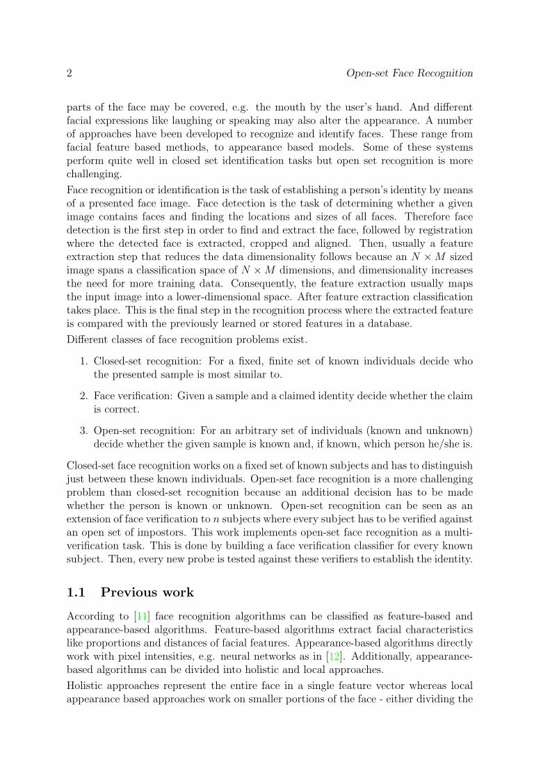
1. Closed-set recognition: For a fixed, finite set of known individuals decide whothe presented sample is most similar to.
2. Face verification: Given a sample and a claimed identity decide whether the claimis correct.
3. Open-set recognition: For an arbitrary set of individuals (known and unknown)decide whether the given sample is known and, if known, which person he/she is.
Closed-set face recognition works on a fixed set of known subjects and has to distinguishjust between these known individuals. Open-set face recognition is a more challengingproblem than closed-set recognition because an additional decision has to be madewhether the person is known or unknown. Open-set recognition can be seen as anextension of face verification to n subjects where every subject has to be verified againstan open set of impostors. This work implements open-set face recognition as a multi-verification task. This is done by building a face verification classifier for every knownsubject. Then, every new probe is tested against these verifiers to establish the identity.
1.1 Previous work
According to [11] face recognition algorithms can be classified as feature-based andappearance-based algorithms. Feature-based algorithms extract facial characteristicslike proportions and distances of facial features. Appearance-based algorithms directlywork with pixel intensities, e.g. neural networks as in [12]. Additionally, appearance-based algorithms can be divided into holistic and local approaches.
Holistic approaches represent the entire face in a single feature vector whereas localappearance based approaches work on smaller portions of the face - either dividing the
Open-set Face Recognition 3
Figure 1: Face recognition tasks as described in [8]
whole face into regions which are analyzed independently or focusing on prominentregions such as eyes or nose.
1.1.1 Holistic approaches
Holistic face recognition approaches analyze the entire face at once. The most well-known holistic approach is the eigenfaces approach [9]. A Karhunen-Loeve transform(KLT) - also known as principal component analysis (PCA) - is applied to a trainingset of previously aligned and cropped faces. Then, the first m principal components(eigenfaces) are selected thereby reducing the dimensionality of the recognition task.Now, new faces can be expressed as a linear combination of this eigenface base socomparing an unknown face with previously learned faces is just a matter of comparingcoefficients that associate with each eigenface. Drawbacks of this approach are itssensitivity to lighting and pose variations as well as registration errors. Fisherfaces [6],[7] is a similar holistic approach that uses Fisher linear discriminant analysis (LDA)for dimensionality reduction. The eigenfaces approach maximizes the overall scatter,whereas fisherfaces uses class information and maximizes the ratio of between-classscatter to within-class-scatter. The eigenfaces approach aims at best reconstruction offace images in a mean square error sense. Fisherfaes on the other hand deals directlywith classification.

4 Open-set Face Recognition
1.1.2 Local appearance-based approaches
It has been found that holistic approaches are more sensitive to lighting and posechanges and suffer from occlusion and changes in facial expression. Therefore local ap-pearance based approaches were introduced. Modular eigenfaces [9] for example thatfocuses on eye and nose regions only for recognition has been shown to outperformthe holistic eigenface approach. Another example that is using local appearance-basedfeatures is [10]. There support vector machines are used as classifiers on local face com-ponents which partially overlap. The local component-based approaches outperformedholistic approaches using support vector machines as well.
1.1.3 Face verification
Face verification plays an important role in secure biometric applications and has beenstudied extensively. It is also important in this work because a multi-verification ap-proach is used to implement open-set face recognition. Support vector machines wereused to implement high-security verification systems, examples are approaches by Jon-sson et al. [17], Kim et al. [19], Lee et al. [20], Phillips [22] and Cardinaux et al.[21].
Phillips [22] applies SVMs to face verification. The work introduces a parametrized de-cision surface in order to optimize the trade-off between the probability of correct verifi-cation PV and false acceptance PF , the decision surface {xεS : wx+b = 0, (w, b)εS×R}is changed to wx + b = ∆, where ∆ allows variation of PV and PF . Classification isperformed in difference space consisting of within-class differences modeling differenceswithin the same class and between-class differences that model differences between dif-ferent classes. Then, the SVM is trained to build a decision surface separating theseclasses. This SVM can be used to estimate similarities between two facial images.
Jonsson et al. [17] employ support vector machines and explore their discriminatorycapabilities. Faces are both represented in principal component and linear discriminantsubspaces for comparison. They show that SVMs can extract the relevant informationand outperform benchmark approaches on non-discriminatory representation but losethis advantage if discriminatory features like those obtained by LDA are used. Unlike[22] this approach uses client-specific support vectors.
Kim et al. [19] build a verification framework considering real-world applicability. Theytry to limit memory consumption and consider easy removal and addition of clients.The approach is based on a feature set comprised of several PCA-based features and anadditional edge map. The work describes the new features as eigenUpper, consisting offorehead, eyes and nose that tries to minimize influence of expression, and eigenTzone,consisting of eyes and nose that tries to compensate illumination. Instead of trainingone SVM per enrolled client an SVM monitor is trained to model an intra-/extra-personsimilarity space on eight different simple similarity measures. By using a similarityspace and a single SVM memory consumption and computational overhead are reduced.
Cardinaux et al. [21] train SVM and MLP classifiers on features consisting of raw-pixelvalues of resized and normalized face images and a skin color distribution vectors. In

Open-set Face Recognition 5
this case the MLP outperformed the SVM approach.
1.1.4 Open-set face recognition
Open Set Face Recognition Using Transduction is one of the few papers [4] that ex-plicitly addresses the issue of open-set recongition.

6 Open-set Face Recognition
2 Methodology
This section gives an overview of the basic principles and techniques used in this work.
2.1 Haar cascade classifiers
Haar cascade classifiers, developed by Viola and Jones (2001) [18], present a fast andefficient object detection framework. The framework utilizes Haar-like features andboosted classifier cascades. Haar-like features are simple rectangle features inspired byHaar basis functions. AdaBoost is then used to select the most promising Haar-likefeatures efficiently. In order to further improve performance a cascaded structure wasintroduced. A cascade is a degenerate decision tree that assesses a limited combinationof features at every stage. Early stages try to reject as many negative samples aspossible while accepting nearly all positive samples. The advantage is then that onlyfew search windows have to descend through the whole cascade.
2.1.1 Haar-like features
Haar-like features are simple rectangle features inspired by Haar basis functions. Com-puted features have advantages over using pixel intensities directly. Although far morerectangle features than pixels exist, once a set of discriminative features has been se-lected they can be evaluated faster and they reduce the classification complexity byutilizing a lower dimensional feature spaces and thus allow better results using a finiteamount of training examples. Examples of these rectangle features can be seen below.
Figure 2: The following sample Haar-like features consist of up to four boxes whosegray value differences are computed
Haar-like features consist of up to four rectangular image regions and they are computedas differences of rectangular image regions. These features can be of arbitrary size andposition within the search window. Therefore even relatively small search windowsyield a large number of possible features.
Albeit being simpler than other possible feature representations Haar-like features haveone distinct advantage. They can be computed very efficiently due to their simplenature. In order to keep computation overhead at a minimum so-called integral imageswere introduced.
Open-set Face Recognition 7
2.1.2 Integral image
In order to compute rectangle features very rapidly the integral image is used. Theintegral image is a different representation of images that allows to compute intensitysums of rectangles very efficiently. Every point of the integral image corresponds tothe sum of all intensities within the rectangle that is spanned from the image origin tothe current point’s location.
The integral image can be calculated according to
ii(x, y) =∑
x′≤x,y′≤y
i(x′, y′) (1)
where x, y are the integral image positions and i(x′, y′) represents the image intensityvalue at (x’, y’). This formula can be computed with a single pass over the im-age by temporarily storing the current row’s intensity sum and referencing previouslycalculated rectangle sums, the row sum being s(x, y) = s(x, y − 1) + i(x, y) and thencalculating the integral image value at (x, y) according to ii(x, y) = ii(x−1, y)+s(x, y).
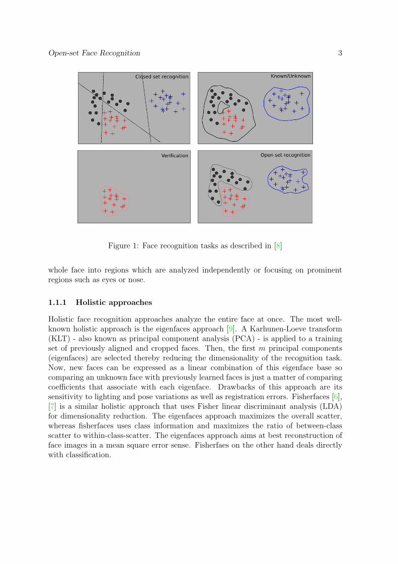
The integral image will quickly provide rectangle intensity sums for rectangles startingat the origin, but arbitrary rectangles also have to be computed. These rectangle sumscan be calculated easily by means of the integral image as can be seen by the illustrationbelow - the empty area on top of and left of the intended rectangle have to be subtractedfrom the large rectangle that spans from top-left to the current point whose area caneasily be obtained from the integral image. Because these subtractions overlap we needto add a small top-left portion where the subtraction occurred twice. Therefore, onlyfour array lookups are needed to calculate the intensity sum of a rectangle.
Figure 3: Integral image representation ii(x; y) is the sum of all pixel intensities con-tained in the box from the upper-left corner to the current point. Computing theintensity sum of an arbitrary box is achieved by subtracting the sum of pixel intensi-ties of boxes B and C from the main box and adding the sum of A, because A, B, Coverlap.
8 Open-set Face Recognition
2.1.3 Boosted classifier cascades
Even rather small search windows yield up to 180,000 possible feature combinations.Therefore an effective feature selection algorithm needs to select the most promisingfeatures. Viola and Jones [18] proposed to use a modified AdaBoost algorithm.
AdaBoost builds strong classifiers from so-called weak classifiers. It combines severalof these weak classifiers via linear combination into a strong classifier that can fulfilla given classification task even though the weak classifiers it consists of need only beslightly better than chance. It does so by selecting the most discriminative featuresgreedily. In the framework presented by Viola and Jones in [18] thresholded Haar-likefeatures are used as weak classifiers. And according to [18] the great challenge is tofind those features that can be combined to form a good classifier.
Consequently, those weak learners are chosen that separate positive and negative exam-ples as good as possible. This is achieved by using a thresholded classification functionthat tries to minimize misclassifications of examples. Thus a weak classifier hj(x) con-sists of a feature fj, a threshold θj and a parity sign pj that indicates the direction ofthe inequality and x being a 24x24 search window:
hj(x) =
{1 if pjfj(x) < pjθj0 otherwise
(2)
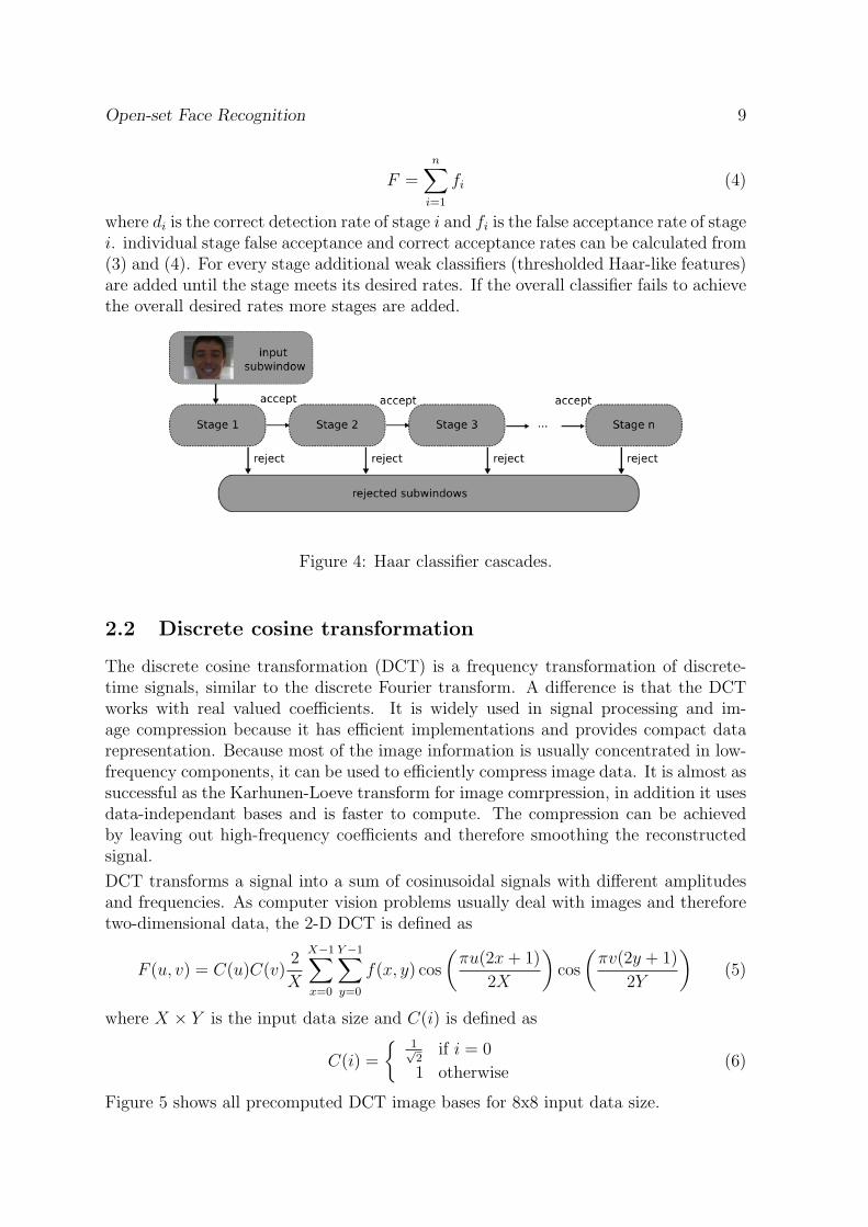
Selecting many features will increase classification performance as many sample detailscan be modeled but at the same time many features lead to higher computation times.That results from the fact that in the current framework all features are evaluatedover every possible search window in the image. To avoid evaluating all selected,discriminating features cascades are introduced. They are basically degenerate decisiontrees where at every stage a search window is either rejected or passed to the next stage,a window is finally accepted if it passes the whole cascade. The idea is to have earlystages that discard many negative samples while still accepting all positive samplesand to have more discriminative stages later that were trained on harder examples.Ideally many easy negative search windows are discarded early on and only hard toclassify windows proceed further through the cascade. Therefore, the entire cascadewill be evaluated in the rare case of positive samples and not for every search windowwhile still retaining all of its discriminative power.
Cascade training is done accordingly. The first stage is usually trained with randomnon-object class negative samples and object class positive samples. The first stagetries to accept nearly 100% positives while rejecting as many negatives as possible.Then the next stage is only trained with the falsely accepted negatives that the firststage missed and this continues through all further stages. Therefore every stage facesa harder classification task than the stage before and thus is better at rejecting falsepositives while still trying to accept nearly all true positives. Now, the overall correctdetection rate D and false detection rate F of a cascade with n stages can computedaccording to
D =n∑i=1
di (3)
Open-set Face Recognition 9
F =n∑i=1
fi (4)
where di is the correct detection rate of stage i and fi is the false acceptance rate of stagei. individual stage false acceptance and correct acceptance rates can be calculated from(3) and (4). For every stage additional weak classifiers (thresholded Haar-like features)are added until the stage meets its desired rates. If the overall classifier fails to achievethe overall desired rates more stages are added.
Figure 4: Haar classifier cascades.
2.2 Discrete cosine transformation
The discrete cosine transformation (DCT) is a frequency transformation of discrete-time signals, similar to the discrete Fourier transform. A difference is that the DCTworks with real valued coefficients. It is widely used in signal processing and im-age compression because it has efficient implementations and provides compact datarepresentation. Because most of the image information is usually concentrated in low-frequency components, it can be used to efficiently compress image data. It is almost assuccessful as the Karhunen-Loeve transform for image comrpression, in addition it usesdata-independant bases and is faster to compute. The compression can be achievedby leaving out high-frequency coefficients and therefore smoothing the reconstructedsignal.
DCT transforms a signal into a sum of cosinusoidal signals with different amplitudesand frequencies. As computer vision problems usually deal with images and thereforetwo-dimensional data, the 2-D DCT is defined as
F (u, v) = C(u)C(v)2
X
X−1∑x=0
Y−1∑y=0
f(x, y) cos
(πu(2x+ 1)
2X
)cos
(πv(2y + 1)
2Y
)(5)
where X × Y is the input data size and C(i) is defined as
C(i) =
{ 1√2
if i = 0
1 otherwise(6)
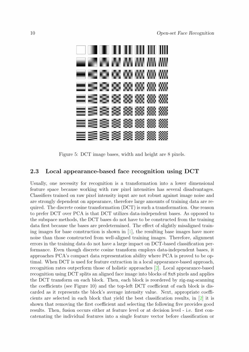
Figure 5 shows all precomputed DCT image bases for 8x8 input data size.
10 Open-set Face Recognition
Figure 5: DCT image bases, width and height are 8 pixels.
2.3 Local appearance-based face recognition using DCT
Usually, one necessity for recognition is a transformation into a lower dimensionalfeature space because working with raw pixel intensities has several disadvantages.Classifiers trained on raw pixel intensity input are not robust against image noise andare strongly dependent on appearance, therefore large amounts of training data are re-quired. The discrete cosine transformation (DCT) is such a transformation. One reasonto prefer DCT over PCA is that DCT utilizes data-independent bases. As opposed tothe subspace methods, the DCT bases do not have to be constructed from the trainingdata first because the bases are predetermined. The effect of slightly misaligned train-ing images for base construction is shown in [1], the resulting base images have morenoise than those constructed from well-aligned training images. Therefore, alignmenterrors in the training data do not have a large impact on DCT-based classification per-formance. Even though discrete cosine transform employs data-independent bases, itapproaches PCA’s compact data representation ability where PCA is proved to be op-timal. When DCT is used for feature extraction in a local appearance-based approach,recognition rates outperform those of holistic approaches [2]. Local appearance-basedrecognition using DCT splits an aligned face image into blocks of 8x8 pixels and appliesthe DCT transform on each block. Then, each block is reordered by zig-zag-scanningthe coefficients (see Figure 10) and the top-left DCT coefficient of each block is dis-carded as it represents the block’s average intensity value. Next, appropriate coeffi-cients are selected in each block that yield the best classification results, in [2] it isshown that removing the first coefficient and selecting the following five provides goodresults. Then, fusion occurs either at feature level or at decision level - i.e. first con-catenating the individual features into a single feature vector before classification or

Open-set Face Recognition 11
classifying locally and then fusing the local decisions.
2.4 Support vector machines
Support vector machines (SVMs) are maximum margin binary classifiers that solve aclassification task using a linear separating hyperplane in a high-dimensional projection-space. This hyperplane is chosen to maximize the distance between positive and neg-ative samples. Real-world problems seldom present linearly separable data, thereforea transformation into a higher-dimensional space is applied before classification withhopes of being able to linearly separate data in the new space. The great advantageis that the hyperplane does not need not be projected down into the original space,instead the classification takes place right in the high-dimensional space implicitly.SVMs are conceptually simple yet powerful and the results are interpretable, all goodreasons to employ SVMs. Further introduction into SVMs can be found in [14] and[15].
2.4.1 Linear classification
Figure 6: Linear classifier and margins - the margin is proportional to the expectedgeneralization ability. Taken from [15].
Let {(x1, y1), (x2, y2), . . . , (xm, ym)} again denote the training data, consisting of atraining vector xi and a corresponding classification class yiε{−1, 1}. Under the as-sumption that the provided data can be separated linearly in an n-dimensional space,we can construct an infinite amount of n − 1-dimensional hyperplanes that correctly

12 Open-set Face Recognition
separate the training data, because there are no restrictions on placement or orienta-tion of the hyperplane as long as the data is correctly classified. The idea of maximummargin classification is then to choose the hyperplane with the maximum separatingmargin between the two classes because it can be expected that this maximum marginhyperplane is best at generalization, i.e. the margin is proportional to generalizationability of the classifier.
A hyperplane can be described as
{xεS : wx+ b = 0, (w, b)εS× R} (7)
and the maximum margin separating hyperplane has to minimize the conditionmini=1...n |wxi + b| = 1 where xi are the training examples. Consequently, the dis-tance between two samples xi and xj relative to the hyperplane can be defined asw·(xi−xj)
‖w‖ . Then the distance between the two classes is 2‖w‖ . So in order to classify
training data correctly the hyperplane can be found by maximizing 2‖w‖ or minimizing
‖w‖2 under the condition
yi(wxi + b) ≥ 1 for i = 1 . . . n, (8)
that guarantees that all samples are correctly classified. This minimization can beachieved using Lagrange multipliers once rewritten into
Lp = L(w, b, a) =1
2‖w‖2 −
n∑i=1
αi(yi(wxi + b)− 1) . (9)
with α1, α2, . . . , αn being Lagrange multipliers. After solving the optimization prob-lem most αi are zero because their conditions are fulfilled. Those xi whose αi > 0are chosen as support vectors to represent the margins, they are the closest vectorsto the hyperplane. Then w can be computed as a linear combination of these αi:w =
∑ni=1 αiyixi.
2.4.2 Soft-margin linear classification
In order to allow a certain number of misclassifications a soft-margin is introduced. Theoptimization condition is changed to yi(wxi + b) ≥ 1− ξi for i = 1 . . . n, ξi ≥ 0, whereξi is the sample xi’s distance from the correct margin, it is sometimes also referred toas slack term. Therefore if ξi > 1 the sample is misclassified, if 0 < ξi < 1 the sampleis correctly classified but within the margin (margin error) and if ξi = 0 the vector lieson the margin. Consequently, the minimization term becomes
minw,b,ξi‖w‖2 + C
(n∑i=1
ξi
)(10)
where C is a weighting parameter that controls the rate of misclassifications - small Cmaximizes the margin, large C yields few misclassifications.
So soft-margin classifiers allow a certain number of misclassifications and can thereforebetter cope with data that is not exactly linearly separable.
Open-set Face Recognition 13
2.4.3 Non-linear classification
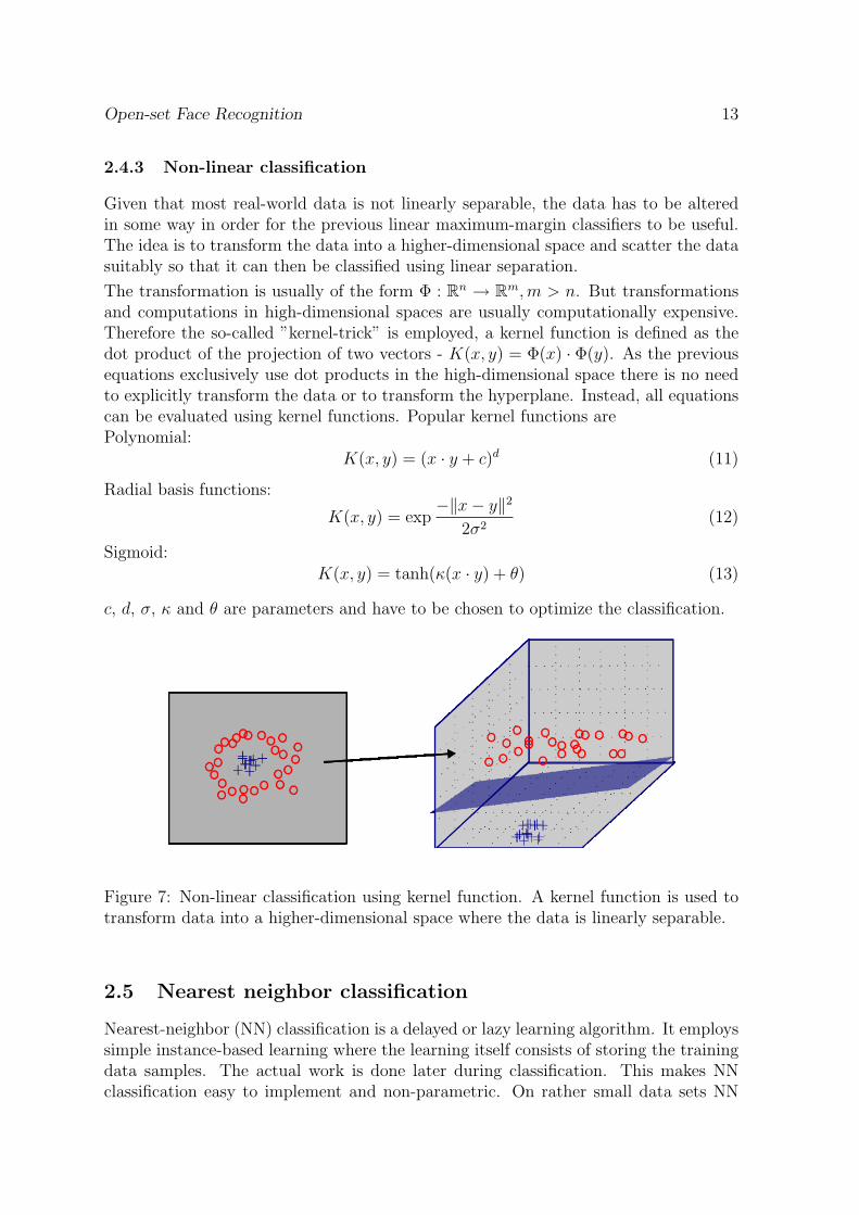
Given that most real-world data is not linearly separable, the data has to be alteredin some way in order for the previous linear maximum-margin classifiers to be useful.The idea is to transform the data into a higher-dimensional space and scatter the datasuitably so that it can then be classified using linear separation.
The transformation is usually of the form Φ : Rn → Rm,m > n. But transformationsand computations in high-dimensional spaces are usually computationally expensive.Therefore the so-called ”kernel-trick” is employed, a kernel function is defined as thedot product of the projection of two vectors - K(x, y) = Φ(x) · Φ(y). As the previousequations exclusively use dot products in the high-dimensional space there is no needto explicitly transform the data or to transform the hyperplane. Instead, all equationscan be evaluated using kernel functions. Popular kernel functions arePolynomial:
K(x, y) = (x · y + c)d (11)
Radial basis functions:
K(x, y) = exp−‖x− y‖2
2σ2(12)
Sigmoid:K(x, y) = tanh(κ(x · y) + θ) (13)
c, d, σ, κ and θ are parameters and have to be chosen to optimize the classification.
Figure 7: Non-linear classification using kernel function. A kernel function is used totransform data into a higher-dimensional space where the data is linearly separable.
2.5 Nearest neighbor classification
Nearest-neighbor (NN) classification is a delayed or lazy learning algorithm. It employssimple instance-based learning where the learning itself consists of storing the trainingdata samples. The actual work is done later during classification. This makes NNclassification easy to implement and non-parametric. On rather small data sets NN

14 Open-set Face Recognition
classification is on par computationally with other classifiers and may even outperformcomplex classification algorithms.
Given the training data {(x1, y1), (x2, y2), . . . , (xm, ym)}, consisting of a training vectorxi and a corresponding classification class yi, and a vector x that is to be classified,NN is defined as
c = argminiε1,...,m
‖x− xi‖ (14)
.
The result is the class of sample xc, namely yc. This approach can easily be extended tok nearest neighbors. In that case, the decision is made by combining the each nearestneighbor’s decision in some way.
Usually, nearest-neighbor classification is performed in an Euclidean space using theEuclidean distance metric, also known as L2 norm. Other norms may be used, such asthe L1 or city-block distance. It is defined as
d(x1, x2) =N∑b=1
|x1[b]− x2[b]| (15)
where xi[b] is the bth component of the vector xi and N is the length of vectors xi.
A detailed evaluation of the use of different distance metrics in nearest-neighbor clas-sification for local appearance-based face recognition is performed in [2]. The paperstates that usually the L1-norm outperforms other norms. Therefore we use L1-normin nearest-neighbor classification later in this work.
2.6 K-Means clustering
The k-means algorithm is an unsupervised learning algorithm that is used to clusterdata, i.e. classify objects into different categories, into k partitions. It was introducedby MacQueen [16] and is related to the expectation-maximization algorithm. In thek-means approach clusters are represented by their respective centroid or mean. Dueto its conceptual simplicity and efficiency it is used widely.
K-means tries to reduce the sum-squared distance of all data-points xj and its associ-ated cluster mean µi. The error term can be formulated as
SSE =k∑i=1
∑xj∈Si
d(xj, µi)2 (16)
where d(x1, x2) denotes the distance between a data-point and a cluster-mean. Gener-ally, Euclidian and city block distance are used as the distance metric.
The simplest form of the algorithm starts by selecting k random cluster means, e.g.by selecting k random data points as initial cluster means. Then, every data point isassigned to its nearest centroid according to the distance function. The next step isto update the centroid locations by calculating the mean of all assigned data pointsto each current cluster. These steps are iterated until either the centroids’ values no

Open-set Face Recognition 15
longer change, until the data points do not switch between clusters or until a certainnumber of iterations is reached.
K-means may in fact converge to local minima. One solution to avoid only locallyoptimal solutions is to start with different random centroids and run the algorithmseveral times.

16 Open-set Face Recognition
3 Open-Set Face Recognition
This chapter covers the implementation and is organized as follows. Section 3.1 de-scribes how the face registration component works, Section 3.2 explains the featureextraction procedure. Then, Section 3.3 introduces the classifiers that were employedand Section 3.4 provides information about the use of additional video-based informa-tion.
3.1 Face registration
Face registration is the task of aligning the faces such that different faces are trans-formed to a common coordinate system. This task is a crucial preparation step forface recognition. Since most recognition algorithms are quite sensitive to even smallchanges in orientation or position correct registration is very important. If registrationfails recognition cannot be performed successfully.
Face registration can be considered as a normalization step and consists of two phases.First, a face detection algorithm needs to find the face. Then, an eye detection algo-rithm is used to detect the eyes. The eye locations are used as reference points, andthe images are transformed so that eye locations in the registered images are the same.
3.1.1 Face detection
Face detection is done by using Haar cascade classifiers. The classifiers were trained onseveral face and randomly chosen non-face images. The detected outline is usually notsuited to be taken directly for recognition. The final Haar cascade classifier output isa fusion of multiple detections that can occur at different scales and slightly differentpositions for same face, so it can be rather crude. Therefore further steps need to betaken.
In order to be able to handle multiple persons appearing and disappearing, in case ofmultiple face detections the largest hit with the least distance from the last detectionis selected.
3.1.2 Eye detection
As stated above, face detection is just a rough first step to estimate face position. Thereturned rectangle can vary significantly in size and sometimes location, a first detectionmay cover just the skin-colored face area, whereas the next detection may cover thewhole face including neck and hair. It is difficult to establish robust recognition ifthe variation between two consequent detections of the same person may already belarger than the overall differences between two totally different people. Therefore, inaddition to face detection, eyes are detected as well to provide more robust cues aboutface orientation and size.
Eye detection is also done using Haar cascade classifiers. Eyes seem to pose a greaterproblem than faces for the Haar cascade classifiers because they contain less discrimi-
Open-set Face Recognition 17
natory intensity features. Fortunately, once a face is detected there are not too manyother similar facial features. Nonetheless, false positive detections may occur aroundthe nose or far more often e.g. on curly hair. Haar cascade detection may fail completelyif the eye-brows are covered by hair. That is because just the eyeball’s appearance byitself contains too few discriminatory information to robustly detect eyes and thereforeadditionally eyebrows were included in training images as there is usually a high con-trast difference between the eye brows and the surrounding area, which improves thedetector.
Additionally, to improve robustness a few checks were included. The eye detection hasto be within the upper half of the face, the left eye must be within the left upper half,and the right eye within the right upper half of the face. In order to minimize thejitter of eye detections the newly detected eye coordinates are compared with the lastdetection and the closest hit is chosen.
If the eye detector fails to detect either eye an educated guess is made based on thecurrent face location and old eye positions. This ensures that infrequent mismatchescan be compensated.
3.1.3 Alignment
After face and eye positions have been established alignment is straight forward. Theimage is rotated and then cropped according to the distance between the eyes. Theoutput of the aligner is a cropped and rotated face image of 128x150 pixels size, thedistance between eyes is 70 pixels and the eyes are located 45 pixels from the top ofthe image. The resulting registered image is then scaled to 64x64 pixels size, the eyelocations in registered images are the same.
3.1.4 Sample augmentation
Imperfect registration may decrease recognition performance but perfect registrationis very hard to achieve and not always possible. The advantage of creating additionalsamples is that a classifier trained with these samples becomes more robust againstregistration variations. This is important because registration in real-world applicationsis usually not perfect. In order to overcome this difficulty an additional processing stepis performed. Before applying the DCT transform to an aligned and cropped faceimage a set of related images are generated by slightly varying detected eye locationsand therefore creating new images with slightly different alignment.
In order to simulate the influence of imprecise registration, each eye’s location is variedindividually by a few pixels in each direction, for example in the 4-neighborhood of thedetection. A variation of the eye location by a single pixel in each direction ({−1, ..., 1}in x direction and {−1, ..., 1} in y direction per eye) yields 24 additional samples.Consequently, 25 times more registered face images are available with just a variationof a single pixel. Increasing the amount of data may cause problems, it may lead tosample data imbalances. So, after creating these additional samples and extractingthe features k-means clustering is applied to reduce the amount of positive samples.
18 Open-set Face Recognition
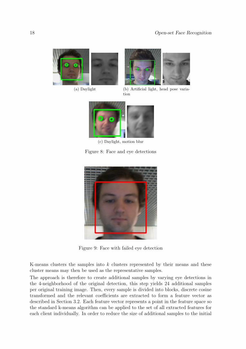
(a) Daylight (b) Artificial light, head pose varia-tion
(c) Daylight, motion blur
Figure 8: Face and eye detections
Figure 9: Face with failed eye detection
K-means clusters the samples into k clusters represented by their means and thesecluster means may then be used as the representative samples.
The approach is therefore to create additional samples by varying eye detections inthe 4-neighborhood of the original detection, this step yields 24 additional samplesper original training image. Then, every sample is divided into blocks, discrete cosinetransformed and the relevant coefficients are extracted to form a feature vector asdescribed in Section 3.2. Each feature vector represents a point in the feature space sothe standard k-means algorithm can be applied to the set of all extracted features foreach client individually. In order to reduce the size of additional samples to the initial

Open-set Face Recognition 19
amount of data, the clustering parameter k is chosen as N25
, where N is the number ofinitial samples and clustering is done using the L1 distance metric. After clustering,the usual training and classification steps can be performed.
3.2 Feature extraction
Every cropped and aligned face image of 64x64 pixels resolution may be interpreted asa single point in a 64x64 dimensional space. But too many training examples wouldbe needed to perform classification in such a high-dimensional space. Therefore thedimensionality of the features has to be reduced. The standard approaches to dimen-sionality reduction include principle component analysis (PCA), linear discriminantanalysis (LDA) and discrete cosine transformation (DCT). DCT has the advantageof utilizing data-independent bases which limit the influence of registration errors be-cause these bases do not have to be constructed from automatically registered inputimages during training. Misaligned training images decrease the performance of sub-space methods because noise is introduced in the basis images, see [2] for examples.OpenCV was used to extract DCT features.
3.2.1 Local DCT coefficients
Every aligned and cropped face image to be classified is first converted into a grayscaleimage of 64x64 pixels and then divided into 8x8 pixel blocks, then DCT is performed oneach of these local blocks. A block size of 8x8 pixels provides a reasonable compromisebetween compression and processing overhead.
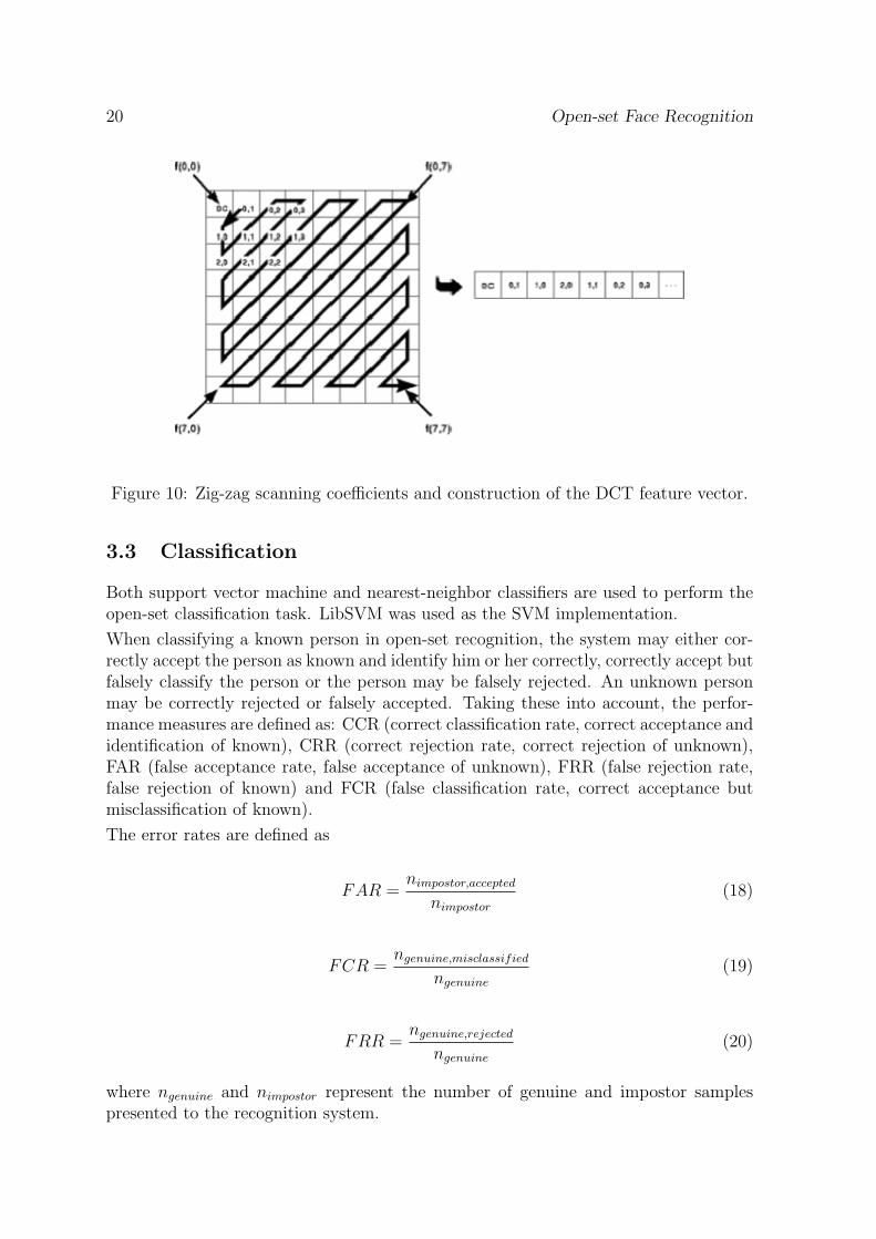
After dividing the image into 8x8 blocks DCT is performed on each block. Then, eachblock’s coefficients are ordered using zig-zag-scanning, see Figure 10. From that sortedlist, the first, so-called DC, component is skipped because it represents the averagepixel intensity of the entire block. The following five coefficients are retained and theremaining coefficients are discarded. Especially these low-frequency coefficients havebeen shown to perform well as features for classification tasks. The process then yieldsfive DCT coefficients for every image block. There are in total local 64 blocks in 64x64input images, so the dimensionality is reduced from 4096 to 320.
3.2.2 Feature normalization
DCT preserves the total image energy of the processed input block, therefore blockswith different brightness levels lead to DCT coefficient with different magnitude values.In order to balance each local block’s contribution to the classification the local featurevector is normalized to unit norm. The magnitude of feature vector f is transformedinto the normalized feature vector fn:
fn =f
||f ||(17)
20 Open-set Face Recognition
Figure 10: Zig-zag scanning coefficients and construction of the DCT feature vector.
3.3 Classification
Both support vector machine and nearest-neighbor classifiers are used to perform theopen-set classification task. LibSVM was used as the SVM implementation.
When classifying a known person in open-set recognition, the system may either cor-rectly accept the person as known and identify him or her correctly, correctly accept butfalsely classify the person or the person may be falsely rejected. An unknown personmay be correctly rejected or falsely accepted. Taking these into account, the perfor-mance measures are defined as: CCR (correct classification rate, correct acceptance andidentification of known), CRR (correct rejection rate, correct rejection of unknown),FAR (false acceptance rate, false acceptance of unknown), FRR (false rejection rate,false rejection of known) and FCR (false classification rate, correct acceptance butmisclassification of known).
The error rates are defined as
FAR =nimpostor,accepted
nimpostor(18)
FCR =ngenuine,misclassified
ngenuine(19)
FRR =ngenuine,rejected
ngenuine(20)
where ngenuine and nimpostor represent the number of genuine and impostor samplespresented to the recognition system.
Open-set Face Recognition 21
3.3.1 SVM based classification
Open-set recognition is a multi-class classification problem, support vector machineson the other hand are binary classifiers. Traditionally, two ways were employed to solvemulti-class problems with SVMs, either a one-vs-one or one-vs-all approach.
The one-vs-one solution works by training m(m−1)2
classifiers to solve an m-class prob-lem. Each classifier is trained to separate two single classes, this is a pairwise approach.
In the one-vs-all approach m classifiers are trained to solve the m-class problem. EachSVM separates one class from all other remaining classes.
This work formulates the open-set recognition problem as a multi-verification task. Asdescribed by McKenna et al. in [8], open-set face recognition can be formulated as aseries of 2-class verification problems. Given a claimed identity, the result of an identityverification is whether the claimed identity is true or false. Given a number of positiveand negative samples it is possible to train a classifier that models the distribution offaces for both cases. In order to carry out open-set recognition, an identity verifieris trained for every one of the n known subjects in the database. Then in order toperform open-set recognition, the probe is presented to each verifier and n verificationsare performed. Once a new probe is presented to the system, it is checked against allclassifiers, if all of them reject, the person is reported as unknown; if one accepts, theperson is accepted with that identity, if more than a single verifier accepts, the identitywith the highest score wins. Scores are inversely proportional to the nearest-neighbordistance. For the n-best list creation, all distances are converted into scores and thena min-max normalization is performed on the list.
The two-class nature of SVM classification lends itself to formulating the open-setrecognition task as a verification problem. Although one-class SVMs exist they werenot used because there is a sufficiently large set of training data that can be used tomodel the class of unknown individuals. Providing samples for both classes allows theSVM classifier to choose the optimal separating support vectors and therefore providea better model of the probability density function than a one-class model that has toestimate the boundary without actually having negative examples.
Since this work focuses on video-based classification, n-best lists are used instead ofa single frame-based score as will be explained later. The advantage of using n-bestlists is that no hard decisions are made immediately so that initial false decisionsmay be revised later. N-best lists are lists containing the n best classification resultsordered by classification score. Therefore scores need to be derived, in case of SVMclassification the score is the distance from the hyperplane. Unlike calibrated sigmoidposterior probabilities as proposed by Platt in [24] these do not represent posteriorprobabilities. In order to reduce variation of distances between frames, the score ismin-max-normalized [25] as
s′i = 1− si − sminsmax − smin
i = 1, 2, ..., n. (21)
This maps scores to [0, 1] and then all scores are renormalized to yield∑n
i=1 s′i = 1 so
that each frame has an equal contribution.

22 Open-set Face Recognition
Training data imbalance consideration
A large set of negative samples, i.e. training samples of unknown clients, is necessaryto capture the large variance of the unknown class in the multi-verification approach.Every recording session consists of roughly 150 frames, unknown people have a singlerecording session which is used for training, whereas four sessions are used for knowntraining. In order to have balanced data, i.e. an equal number of positive (known) andnegative (unknown) training images we would need to have as many recordings of thesingle known person as from all unknowns combined. Therefore, if we use four sessionper known for training with ≈ 600 frames against 20 unknown individuals with ≈ 150frames each (≈ 3000 total) we would have a 1:5 imbalance. In case of only a singleavailable session per known the imbalance is 1:20.
This problem was tackled by undersampling the unknown sequences here. Under-sampling works by selecting only every nth frame to train the classifier if there is animbalance of 1:n.
As Akbani et al. state in [13] undersampling shows a significant performance gain.Undersampling is inferior to the proposed SDC algorithm presented in [13] but outper-forms pure SVM classification on unbalanced datasets.
3.3.2 Nearest-neighbor based classification
The nearest-neighbor based classification method uses the same sort of multi-verificationapproach. Again, for every person to be recognized an individual classifier is trained.
The problem is that the samples of some subjects may have a larger variance in distancethan the samples of some other individual. Nonetheless, we would like to use a commonthreshold that can be tuned globally - for example by finding the equal error rate.
Each nearest-neighbor classifier calculates a normalized distance, this normalized dis-tance is simply shifted by the mean and divided by the standard deviation that is basedon the distances obtained on the training samples:
d′ =d− µciσci
(22)
where d is the distance of the classifier’s input vector to the nearest training sample inclass ci and µci and σci are mean and variance of distances of class ci estimated usingthe training data. If this normalized distance is lower than the global threshold theprobe sample is accepted by the verifier.
3.4 Video information incorporation
This section explains how additional information from video sequences is used to im-prove classification performance.

Open-set Face Recognition 23
3.4.1 Temporal fusion with progressive scores
Since a person’s identity does not change during the video capture, one may try toenforce temporal consistency. In order to make it possible to revise a preliminarydecision later on, instead of relying on a single classification result for every frame ann-best list is used. N-best lists store the first n highest ranked results, n may be chosenfreely, n = 3 was used in this work. Then, for each recognized identity a cumulatedscore is stored that develops over time.
First, the frame n-best list is computed as described in Section 3.3.1 - scores of allaccepting classifiers are gathered into a list, that list is min-max-normalized and thenrenormalized so that the sum of all entries is 1. Then, the scores of the current frameare added to sequence scores. Then, a decision may be made based on sequence scores.Given enough time the real identity should accumulate the highest score because itshould have highest individual frame scores and should have most acceptances.
If there is no face detection over multiple frames in the live system the cumulatedscores are reset because it is assumed that the person has left. Resetting scores allowsthe whole process to restart once another person is located.

24 Open-set Face Recognition
4 Experiments
This section presents the data set and the experiments that were conducted on thedata.
The following section is organized as follows: first the data set is described, then theopen-set face recognition performance of both nearest neighbor and SVM-based base-line systems is compared. After evaluating these baseline systems further optimizationsare introduced and evaluated.
4.1 Experimental setup
The experiments were conducted on a data set that was recorded between Januaryand May 2007. The data set consists of real-world data collected in a wide hallway infront of an office. The system consists of a portable laptop computer and a connectedwebcam that was used to capture short video sequences of the subjects.
The following experiments were performed on an implementation based on LibSVM forSVM-based classification. The SVM parameters were chosen by performing a simplegrid search to find the optimal combination of parameters that yield the best results onan independent cross-validation set based on the FRGC data. The parameter valuesare listed in Table 1.
SVM parametersSVM type C-SVM classifcationSVM kernel Polynomial (γxixj + coef0)d
Polynomial degree d 2γ 2C 32coef0 0ε 10−10
Table 1: SVM parameters
The nearest-neighbor-based classification was performed using the L1 distance metricas supported by results from Ekenel and Stiefelhagen [2].
4.2 Data set
55 people were recorded in front of the office. Lighting was natural or artificial, de-pending on the time of the day. These recordings were split into two groups, a groupof known people and a group of unknown people. From now on, we will use the termknown for those subjects that are added to the database during training, i.e. thoseprobes that have mates in the gallery (or database), unknown will refer to subjectswho are not present in the gallery.

Open-set Face Recognition 25
Each recording session consists of approximately 150 registered frames, i.e. frames inwhich both face and eyes were detected. The recordings are split into training andtesting data. Recordings were executed over a series of four months, so some sessionsare months apart.
Different sets of data were used for training and testing. Known people’s recordingwere split into training and testing sessions which do not overlap. Unknown subjectsused for training are different from those used for testing.
Different experiments required slightly different partitionings of the data, please referto each experiment for a short explanation of the corresponding data set. Dependingon the experiment, either two or four training sessions were used to train known people.25 clients’ sessions were used as unknown training data, the remaining known sessionsand 20 different unknown clients were used for testing.
26 Open-set Face Recognition
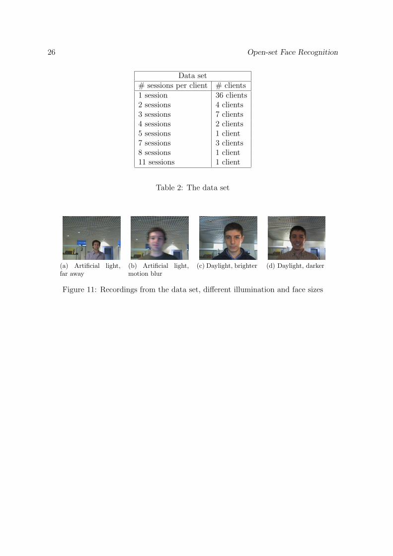
Data set# sessions per client # clients1 session 36 clients2 sessions 4 clients3 sessions 7 clients4 sessions 2 clients5 sessions 1 client7 sessions 3 clients8 sessions 1 client11 sessions 1 client
Table 2: The data set
(a) Artificial light,far away
(b) Artificial light,motion blur
(c) Daylight, brighter (d) Daylight, darker
Figure 11: Recordings from the data set, different illumination and face sizes
Open-set Face Recognition 27
4.3 Open-set face recognition performance
In this subsection, the open-set identification performance of the proposed system is an-alyzed. SVM-based and nearest-neighbor-based classification approaches are comparedand contributions of error types are analyzed based on a baseline system.
4.3.1 Comparison of baseline SVM-based and NN-based open-set facerecognition
The types of errors that can occur during open-set recognition are explained in Section3.3 and defined in Equations 18, 19, 20.
In open-set recognition three error terms, namely FAR, FRR and FCR, have to betraded off against each other and it is not possible to minimize them at the same time.Therefore the equal error rate (EER) performance measure is employed as a combinederror rate measure.
The EER can be found by choosing a threshold for which
FAR = FRR + FCR. (23)
Support vector machines automatically minimize the overall error and try to find theglobal minimum. Therefore if the decision hyperplane is not altered these errors areall automatically minimized. Nonetheless, it may be desirable to fine-tune the system.Depending on the intended use of the system - either for pure recognition or secureapplications - it may be desirable to reduce the number of false rejections and falseclassifications or the number of false acceptances. The ROC curve for SVM-basedclassification was created by using a parametrized decision surface as introduced byPhillips [22]. The decision hyperplane {xεS : wx + b = 0, (w, b)εS × R} is modifiedto wx + b = ∆, where ∆ allows to adjust the false acceptance rate and the correctclassification rate accordingly.
Nearest-neighbor-based classification does not automatically yield the best perfor-mance, a good threshold value has to be selected first. As the nearest-neighbor-basedclassification uses normalized distances a global threshold can be used, the thresholddefines the maximum distance of a test sample to the closest stored training sample ofa given class up to where this test sample is accepted as known. This global thresholdis chosen to satisfy EER criterion.
4.3.2 Performance comparison
This subsection compares open-set classification performance of nearest-neighbor andSVM-based classification. The classification results reported in Table 4 and Table 5were obtained using the data explained in Table 3 and the baseline algorithm usingframe-based classification and undersampling.
Nearest-neighbor-based classification

28 Open-set Face Recognition
Training dataKnown 5 subjects 4 sessions and ≈ 600 frames per personUnknown 25 subjects 1 session, 30 frames per subject
Testing dataKnown 5 subjects 3 – 7 sessions per person and 3646 frames overallUnknown 20 subjects 1 session per person and 3563 frames overall
Table 3: Data set for open-set performance experiments
Classification CCR FRR FAR CRR FCRFrame-based 81.6 % 15.5 % 17.8 % 82.2 % 2.9 %
Table 4: Nearest-neighbor classification results
The above results were obtained using a global threshold of 2.37 that was chosen usingthe equal error rate criterion as in Equation 23.
SVM-based classification
Classification CCR FRR FAR CRR FCRFrame-based 90.9 % 8.6 % 8.5 % 91.5 % 0.5 %
Table 5: SVM classification results, with parametrized hyperplane ∆ = −0.12
The SVM-based classification results were calculated using ∆ = −0.12 for the para-metric hyperplane, according to EER criterion.
Table 4 and Table 5 show that SVM-based classification outperforms nearest-neighborclassification. Studies like [17] suggest that support vector machines perform well inextracting relevant discriminatory information. The nearest-neighbor-based classifica-tion could be further optimized by employing client-specific thresholds and determiningindividual thresholds by means of the EER criterion for each client.
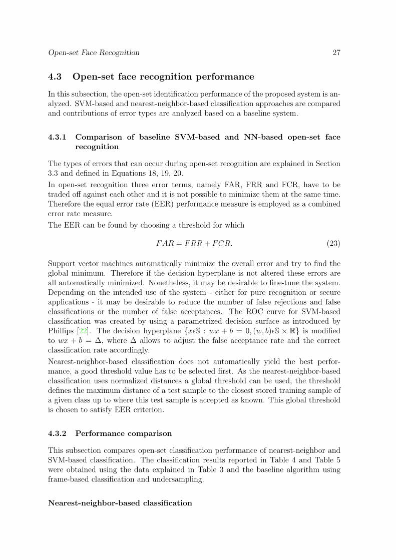
Receiver Operating Characteristic (ROC) curves for both SVM- and nearest-neighbor-based classification are given in Figure 12. The ROC curve plots the correct classi-fication rate against the percentage of impostors accepted by the system. In Figure12, the FAR is represented as the value on the x-axis and correct classification rate isplotted on the y-axis.
Figure 12 a) and b) allows to examine the errors made during classification more closely.The individual contributions of the FRR and FCR can be seen from the graphs. Figure12 shows that at the point of equal error the SVM-based classifier outperforms the NN-based classifier as the CCR is higher.
Open-set Face Recognition 29
0.1 0.2 0.3 0.4 0.5 0.6 0.7 0.8 0.9 10
0.1
0.2
0.3
0.4
0.5
0.6
0.7
0.8
0.9
1
False Acceptance Rate
Cor
rect
Cla
ssifi
catio
n R
ate
FRR
FCR
EER
(a) SVM Receiver Operating Characteristics curve
0 0.1 0.2 0.3 0.4 0.5 0.6 0.7 0.8 0.9 10
0.1
0.2
0.3
0.4
0.5
0.6
0.7
0.8
0.9
1
False Acceptance Rate
Cor
rect
Acc
epta
nce
Rat
e
FRR
FCR
EER
(b) Nearest-neighbor Receiver Operating Characteristics curve
Figure 12: Receiver Operating Characteristics curves

30 Open-set Face Recognition
4.4 Further experiments
This section describes further experiments that were conducted to analyze the per-formance of the proposed system. Unless otherwise stated, SVM-based classificationwas performed using the frame-based baseline approach without optimizations, thehyperplane parameter was kept at δ = 0.
4.4.1 Influence of the number of training sessions
The number of training sessions has an influence on the classification results. Themore training sessions are used the more likely is a good coverage of different poses andlighting conditions. This results in a better client model with more correct acceptancesand less false rejections.
The results in Table 6 were generated using frame-based classification without anyprogressive accumulation of scores. The data set used is described in Table 3. Foursessions were set aside for training of which not all were used depending on the desiredamount of training sessions. Therefore multiple combinations of training sessions arepossible if less than the maximum of four sessions are used for training. In orderto obtain meaningful results, all possible combinations were generated - 1024 for asingle training session, 7776 and 1024 for two and three training sessions and only asingle combination for four training sessions per person. Of these, thirty combinations,if available, were randomly selected for every run. Table 6 reports the mean (µ) ofthe classification rates and their standard deviation (σ) that were computed from theresults of each of these thirty combinations for every run.
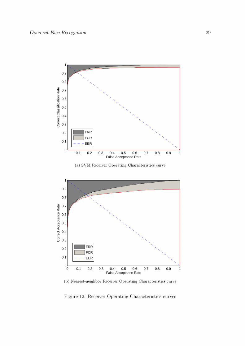
Table 6 and Figure 4.4.1 show that the classification results improve when more datais available. Figure 4.4.1 plots average classification rates and standard deviations fordifferent number of training sessions. More training data covers a greater range ofvariations of the subject in pose, illumination and expression and allows the classifierto better model the subject.
Trainingsessions µCCR σCCR µFRR σFRR µFAR σFAR µCRR σCRR µFCR σFCR1 sess. 29.0 % 8.6 % 71.0 % 8.6 % 0.3 % 0.2 % 99.7 % 0.2 % 0.1 % 0.1 %2 sess. 57.0 % 12.1 % 42.8 % 12.1 % 1.5 % 1.2 % 98.5 % 1.2 % 0.2 % 0.1 %3 sess. 73.8 % 7.8 % 25.8 % 7.8 % 2.6 % 1.1 % 97.4 % 1.1 % 0.4 % 0.1 %4 sess. 87.2 % 0.0% 12.5 % 0.0% 3.7 % 0.0% 96.3 % 0.0% 0.3 % 0.0%
Table 6: Influence of the number of training sessions
4.4.2 Influence of the number of subjects
In order to explore the influence of the number of known subjects in the trainingdatabase the following tests were conducted. Again, frame-based classification wasused and the results can be boosted by using progressive scores.
Open-set Face Recognition 31
1 2 3 40
10
20
30
40
50
60
70
80
90
100
Number of Training Sessions
Cla
ssifi
catio
n R
ate
CCR
FRR
FAR
CRR
FCR
Figure 13: Development of classification scores with number of training sessions. SeeTable 6.
In order to evaluate the influence of the number of known subjects the system canrecognize additional data had to be collected.
Training dataKnown up to 9 subjects 4 sessions per personUnknown 25 subjects 1 session, 30 frames per subject
Testing dataKnown up to 9 subjects 2 sessions per personUnknown 20 subjects 1 session per person
Table 7: Data set for testing the influence of the number of subject
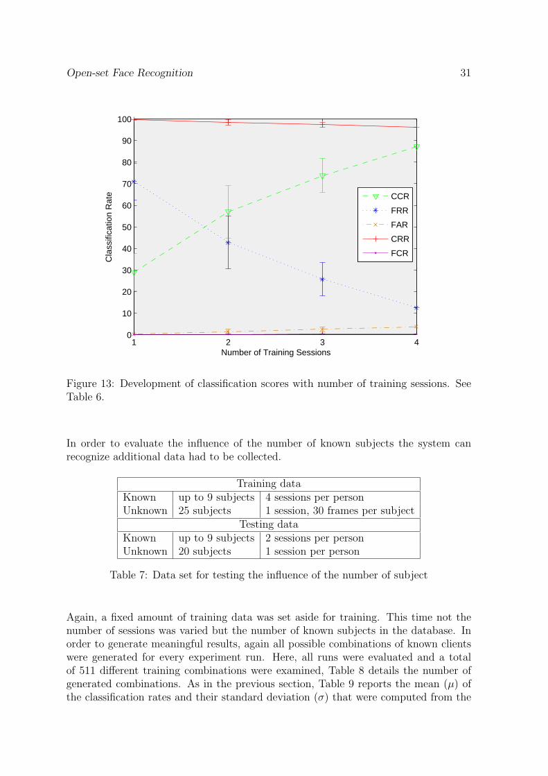
Again, a fixed amount of training data was set aside for training. This time not thenumber of sessions was varied but the number of known subjects in the database. Inorder to generate meaningful results, again all possible combinations of known clientswere generated for every experiment run. Here, all runs were evaluated and a totalof 511 different training combinations were examined, Table 8 details the number ofgenerated combinations. As in the previous section, Table 9 reports the mean (µ) ofthe classification rates and their standard deviation (σ) that were computed from the
32 Open-set Face Recognition
results of each of these combinations for every run.
Due to limited available data only tests with up to nine known subjects could beperformed. Security applications on the other hand have to recognize hundreds ofknown people but that is not the objective of this work. Table 7 explains the dataset that was used in this experiment. Figure 4.4.2 displays the change in classificationperformance as more known subjects are added to the gallery. Table 9 presents thesame results in numeric form and shows that CCR is mostly consistent on average withup to nine known subjects, the CRR decreases slightly as more subjects are added.
# Known subjects # combinations1 known id 92 known ids 363 known ids 844 known ids 1265 known ids 1266 known ids 847 known ids 368 known ids 99 known ids 1Overall 511
Table 8: Number of examined combinations
Subjects µCCR σCCR µFRR σFRR µFAR σFAR µCRR σCRR µFCR σFCR1 subj. 80.9 % 19.4 % 19.1 % 19.4 % 1.1 % 0.9 % 98.9 % 0.9 % 0.0 % 0.0 %2 subj. 80.4 % 12.9 % 19.4 % 12.8 % 2.1 % 1.2 % 97.9 % 1.2 % 0.2 % 0.5 %3 subj. 80.5 % 9.6 % 19.1 % 9.5 % 3.1 % 1.4 % 96.9 % 1.4 % 0.4 % 0.6 %4 subj. 80.8 % 7.5 % 18.6 % 7.3 % 4.0 % 1.4 % 96.0 % 1.4 % 0.6 % 0.6 %5 subj. 80.4 % 6.0 % 18.9 % 5.8 % 5.2 % 1.4 % 94.8 % 1.4 % 0.7 % 0.6 %6 subj. 81.1 % 4.8 % 18.0 % 4.6 % 6.0 % 1.4 % 94.0 % 1.4 % 1.0 % 0.5 %7 subj. 80.7 % 2.9 % 18.8 % 2.6 % 7.9 % 0.3 % 92.1 % 0.3 % 0.6 % 0.3 %8 subj. 79.6 % 0.5 % 18.9 % 0.4 % 8.4 % 0.4 % 91.6 % 0.4 % 1.6 % 0.1 %9 subj. 80.6 % 0.0 % 17.8 % 0.0 % 9.1 % 0.0 % 90.9 % 0.0 % 1.5 % 0.0 %
Table 9: Influence of the number of training sessions
4.4.3 Influence of time span between training and testing
As data was recorded over a time span of four months another interesting experimentwould be to assess the influence of the period of time between training and testing onthe performance. For most knowns there were different sessions which were recorded
Open-set Face Recognition 33
1 2 3 4 5 6 7 8 9
0
20
40
60
80
100
120
Number of Subjects
Cla
ssifi
catio
n R
ate
CCR
FRR
FAR
CRR
FCR
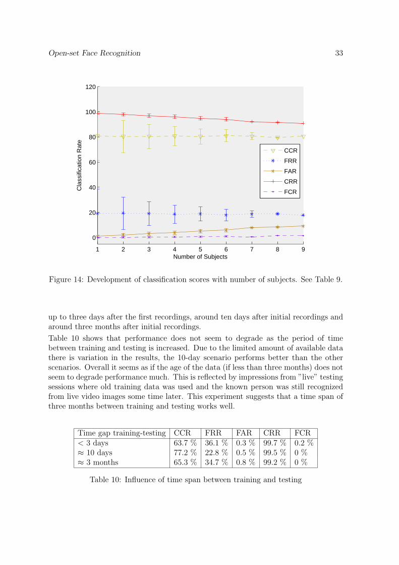
Figure 14: Development of classification scores with number of subjects. See Table 9.
up to three days after the first recordings, around ten days after initial recordings andaround three months after initial recordings.
Table 10 shows that performance does not seem to degrade as the period of timebetween training and testing is increased. Due to the limited amount of available datathere is variation in the results, the 10-day scenario performs better than the otherscenarios. Overall it seems as if the age of the data (if less than three months) does notseem to degrade performance much. This is reflected by impressions from ”live” testingsessions where old training data was used and the known person was still recognizedfrom live video images some time later. This experiment suggests that a time span ofthree months between training and testing works well.
Time gap training-testing CCR FRR FAR CRR FCR< 3 days 63.7 % 36.1 % 0.3 % 99.7 % 0.2 %≈ 10 days 77.2 % 22.8 % 0.5 % 99.5 % 0 %≈ 3 months 65.3 % 34.7 % 0.8 % 99.2 % 0 %
Table 10: Influence of time span between training and testing
34 Open-set Face Recognition
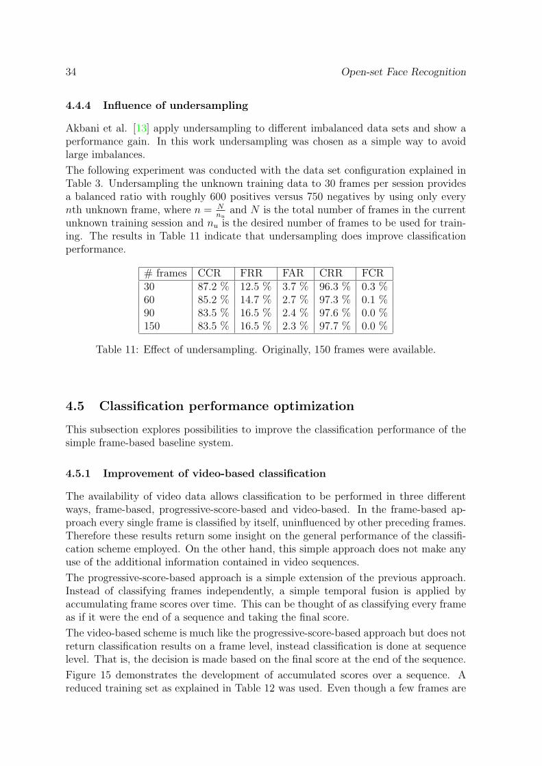
4.4.4 Influence of undersampling
Akbani et al. [13] apply undersampling to different imbalanced data sets and show aperformance gain. In this work undersampling was chosen as a simple way to avoidlarge imbalances.
The following experiment was conducted with the data set configuration explained inTable 3. Undersampling the unknown training data to 30 frames per session providesa balanced ratio with roughly 600 positives versus 750 negatives by using only everynth unknown frame, where n = N
nuand N is the total number of frames in the current
unknown training session and nu is the desired number of frames to be used for train-ing. The results in Table 11 indicate that undersampling does improve classificationperformance.
# frames CCR FRR FAR CRR FCR30 87.2 % 12.5 % 3.7 % 96.3 % 0.3 %60 85.2 % 14.7 % 2.7 % 97.3 % 0.1 %90 83.5 % 16.5 % 2.4 % 97.6 % 0.0 %150 83.5 % 16.5 % 2.3 % 97.7 % 0.0 %
Table 11: Effect of undersampling. Originally, 150 frames were available.
4.5 Classification performance optimization
This subsection explores possibilities to improve the classification performance of thesimple frame-based baseline system.
4.5.1 Improvement of video-based classification
The availability of video data allows classification to be performed in three differentways, frame-based, progressive-score-based and video-based. In the frame-based ap-proach every single frame is classified by itself, uninfluenced by other preceding frames.Therefore these results return some insight on the general performance of the classifi-cation scheme employed. On the other hand, this simple approach does not make anyuse of the additional information contained in video sequences.
The progressive-score-based approach is a simple extension of the previous approach.Instead of classifying frames independently, a simple temporal fusion is applied byaccumulating frame scores over time. This can be thought of as classifying every frameas if it were the end of a sequence and taking the final score.
The video-based scheme is much like the progressive-score-based approach but does notreturn classification results on a frame level, instead classification is done at sequencelevel. That is, the decision is made based on the final score at the end of the sequence.
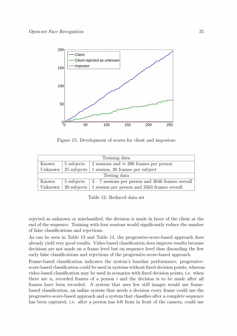
Figure 15 demonstrates the development of accumulated scores over a sequence. Areduced training set as explained in Table 12 was used. Even though a few frames are
Open-set Face Recognition 35
0 50 100 150 200 2500
50
100
150
200
Client
Client rejected as unknown
Impostor
Figure 15: Development of scores for client and impostors
Training dataKnown 5 subjects 2 sessions and ≈ 300 frames per personUnknown 25 subjects 1 session, 30 frames per subject
Testing dataKnown 5 subjects 3 – 7 sessions per person and 3646 frames overallUnknown 20 subjects 1 session per person and 3563 frames overall
Table 12: Reduced data set
rejected as unknown or misclassified, the decision is made in favor of the client at theend of the sequence. Training with four sessions would significantly reduce the numberof false classifications and rejections.
As can be seen in Table 13 and Table 14, the progressive-score-based approach doesalready yield very good results. Video-based classification does improve results becausedecisions are not made on a frame level but on sequence level thus discarding the fewearly false classifications and rejections of the progressive-score-based approach.
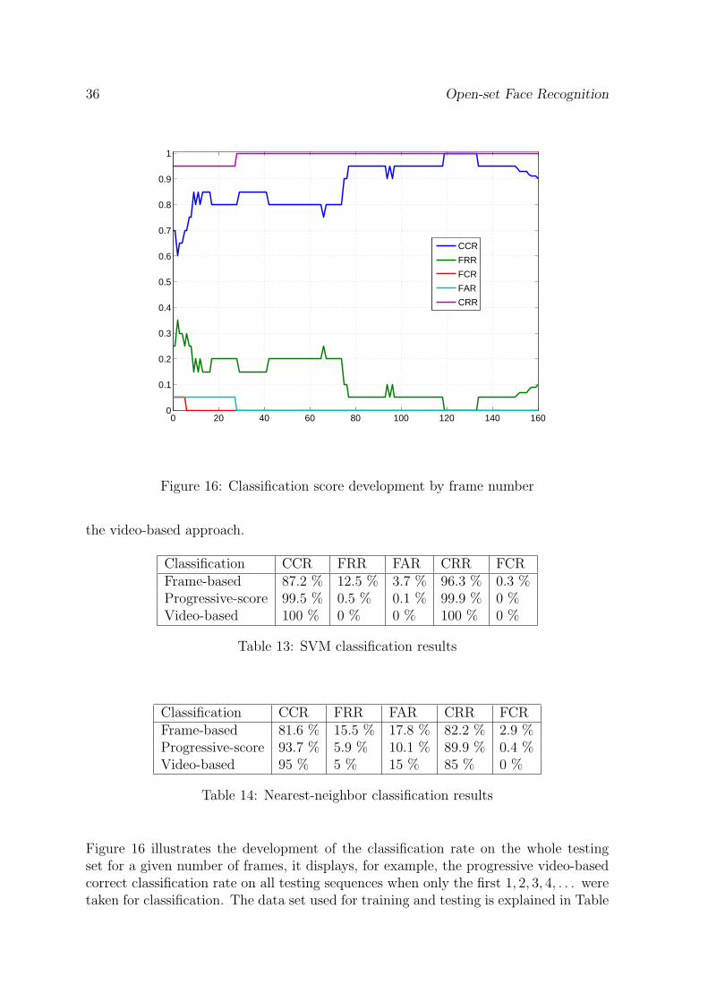
Frame-based classification indicates the system’s baseline performance, progressive-score-based classification could be used in systems without fixed decision points, whereasvideo-based classification may be used in scenarios with fixed decision points, i.e. whenthere are ni recorded frames of a person i and the decision is to be made after allframes have been recorded. A system that uses few still images would use frame-based classification, an online system that needs a decision every frame could use theprogressive-score-based approach and a system that classifies after a complete sequencehas been captured, i.e. after a person has left from in front of the camera, could use
36 Open-set Face Recognition
0 20 40 60 80 100 120 140 1600
0.1
0.2
0.3
0.4
0.5
0.6
0.7
0.8
0.9
1
CCR
FRR
FCR
FAR
CRR
Figure 16: Classification score development by frame number
the video-based approach.
Classification CCR FRR FAR CRR FCRFrame-based 87.2 % 12.5 % 3.7 % 96.3 % 0.3 %Progressive-score 99.5 % 0.5 % 0.1 % 99.9 % 0 %Video-based 100 % 0 % 0 % 100 % 0 %
Table 13: SVM classification results
Classification CCR FRR FAR CRR FCRFrame-based 81.6 % 15.5 % 17.8 % 82.2 % 2.9 %Progressive-score 93.7 % 5.9 % 10.1 % 89.9 % 0.4 %Video-based 95 % 5 % 15 % 85 % 0 %
Table 14: Nearest-neighbor classification results
Figure 16 illustrates the development of the classification rate on the whole testingset for a given number of frames, it displays, for example, the progressive video-basedcorrect classification rate on all testing sequences when only the first 1, 2, 3, 4, . . . weretaken for classification. The data set used for training and testing is explained in Table

Open-set Face Recognition 37
3. Figure 16 shows that after ten frames the correct classification rate is except for oneoccasion above 80% and false acceptance rate is at or below 5%.
4.5.2 Sample augmentation
As previously stated, registration plays an important role. The less precise the regis-tration process is, the more the classification performance decreases. But, it cannotbe assumed that registration is perfect. One scheme to overcome this was proposedin [3]. The approach is to generate artificial, augmented samples by deliberately ma-nipulating the alignment. This can be done by shifting the detected eye coordinatesin the 4-neighborhood around the original detection of the original image. As thatis done on the original image the actual shift of eye positions in the registered imagedepends on the scale of the original face size because it is enlarged/shrinked to 64x64pixels in the process of registration. Alternating eye coordinates in the 4-neighborhoodyields 24 additional samples for every original frame, thus 25-fold amount of data. Inorder to reduce the amount of data again these samples were clustered with k-means.For a total of n original frames that were augmented, k = n
25was chosen in order to
be able to train with the original amount of available data. The experiment resultsin Table 15 were obtained with the data set configuration explained in Table 12 thatuses two training sessions per known. The results in Table 16 were obtained by usingthe data set configuration in Table 3 that uses four training sessions per known. Bothexperiments show improved results.
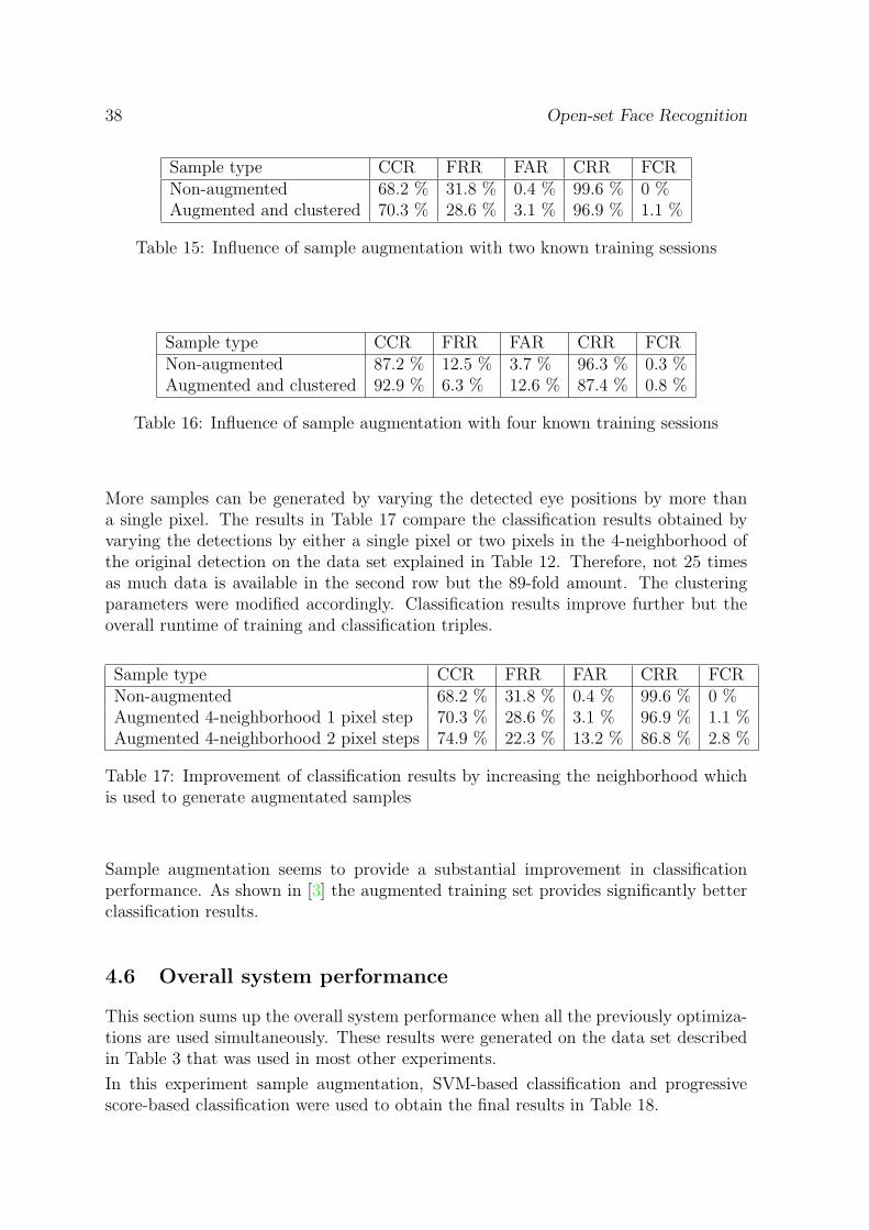
38 Open-set Face Recognition
Sample type CCR FRR FAR CRR FCRNon-augmented 68.2 % 31.8 % 0.4 % 99.6 % 0 %Augmented and clustered 70.3 % 28.6 % 3.1 % 96.9 % 1.1 %
Table 15: Influence of sample augmentation with two known training sessions
Sample type CCR FRR FAR CRR FCRNon-augmented 87.2 % 12.5 % 3.7 % 96.3 % 0.3 %Augmented and clustered 92.9 % 6.3 % 12.6 % 87.4 % 0.8 %
Table 16: Influence of sample augmentation with four known training sessions
More samples can be generated by varying the detected eye positions by more thana single pixel. The results in Table 17 compare the classification results obtained byvarying the detections by either a single pixel or two pixels in the 4-neighborhood ofthe original detection on the data set explained in Table 12. Therefore, not 25 timesas much data is available in the second row but the 89-fold amount. The clusteringparameters were modified accordingly. Classification results improve further but theoverall runtime of training and classification triples.
Sample type CCR FRR FAR CRR FCRNon-augmented 68.2 % 31.8 % 0.4 % 99.6 % 0 %Augmented 4-neighborhood 1 pixel step 70.3 % 28.6 % 3.1 % 96.9 % 1.1 %Augmented 4-neighborhood 2 pixel steps 74.9 % 22.3 % 13.2 % 86.8 % 2.8 %
Table 17: Improvement of classification results by increasing the neighborhood whichis used to generate augmentated samples
Sample augmentation seems to provide a substantial improvement in classificationperformance. As shown in [3] the augmented training set provides significantly betterclassification results.
4.6 Overall system performance
This section sums up the overall system performance when all the previously optimiza-tions are used simultaneously. These results were generated on the data set describedin Table 3 that was used in most other experiments.
In this experiment sample augmentation, SVM-based classification and progressivescore-based classification were used to obtain the final results in Table 18.

Open-set Face Recognition 39
CCR FRR FAR CRR FCROverall system performance 99.6 % 0.2 % 0.2 % 94.2 % 5.8 %
Table 18: Overall system performance using sample augmentation, SVM-based classi-fication, progressive score-based classification
4.7 System runtime performance
This section will present training and testing times of the proposed system. Theruntimes were measured on an Intel Quadcore Xeon 3.00GHz with 2 GB RAM. Thetests were performed on the full dataset as reported in table 3. The base SVM-basedclassification algorithm with frame-based classification was used. The system runs inreal-time, even on much slower laptop computers.
Classification time is 14ms on average including face detection, registration and classi-fication with 5 known subjects trained.
Table 19: System component’s runtime performance
Operation number of executions average runtimeAdding known training samples 1 2 msAdding unknown training samples 1 269 msSVM training 1 21470 msImage preprocessing 10541 < 1 msSVM classification time 7210 14 msClustering of augmented samples 1 359064 ms
Table 19 details the runtime of system components. Training new clients is the singlemost time-consuming procedure. Training five subjects with around 600 frames eachtakes about 21.5 secs. After training, classification can be performed in about 14 ms,excluding image frame capturing but including all preprocessing. The algorithm issufficiently fast to be run on laptop computers in real-time.
Sample augmentation improves the classification results but also imposes a trainingoverhead for generating and clustering the additional samples. When sample augmen-tation is used the generation of new samples and clustering add an additional overheadof about 6 minutes to the training time. Once the clustering is performed there is nofurther performance decrease.

40 Open-set Face Recognition
5 Conclusion
This work presents a fully automatic system for open-set face identification. A multi-verification based approach was chosen and nearest-neighbor and support vector ma-chine classifiers were employed. The classification is based on local features extractedusing discrete cosine transform. Local features were extracted from image blocks byDCT and concatenated into a feature vector that was additionally normalized.
Experiments were conducted on a data set that was collected for this study. We foundthat support vector machines outperform the nearest-neighbor classifier which has beenshown to be a good classifier in closed-set recognition as reported in [1]. Nearest-neighbor-based classification produced quite good results as well, probably due to therather large amount of available data.
The performance of the proposed system could be further improved, especially bysample augmentation which increases training time but yields much improved results.Video-based classification and progressive scores also significantly improved the per-formance. The approach seems to work for larger sets of trained identities but furtherinvestigation is necessary to determine the performance with more than ten clients.From the experimental results it has been observed that the system copes well with atime gap of three months between recording of training and testing data.
The approach worked well in the designated scenario. It seems to cope well withillumination changes. Different poses seem to be a greater problem. Future workis necessary to improve the handling of different viewing angles in order to furtherimprove results.

Open-set Face Recognition 41
References
[1] H.K. Ekenel, R. Stiefelhagen. Local Appearance-based Face Recognition UsingDiscrete Cosine Transform. 13th European Signal Processing Conference (EU-SIPCO 2005). Antalya, Turkey, 2005.
[2] H.K. Ekenel, R. Stiefelhagen. Analysis of Local Appearance-based Face Recogni-tion: Effects of Feature Selection and Feature Normalization. CVPR BiometricsWorkshop, New York, USA, June 2006.
[3] Johannes Stallkamp. Video-based Face Recognition Using Local Appearance-basedModels. Diploma Thesis, November 2006
[4] F. Li and H. Wechsler. Open Set Face Recognition Using Transduction IEEETransactions on Pattern Analysis and Machine Intelligence. 27(11), November2005.
[5] M. Turk and A. Pentland. Eigenfaces for recognition. Journal of Cognitive Science,pp. 71–86, 1991.
[6] W. Zhao, R. Chellappa and P.J. Phillips. Subspace linear discriminant analysisfor face recognition. UMD, 1999.
[7] P.N. Belhumeur, J.P. Hespanha and D.J. Kriegman. Eigenfaces vs. Fisherfaces:Recognition Using Class Specific Linear Projection. IEEE Transactions on PatternAnalysis and Machine Intelligence, 19(7): 711 – 720, 1997
[8] S. McKenna, S. Gong and Y. Raja. Face Recognition in Dynamic Scenes. Proceed-ings of British Machine Vision Conference, 1997.
[9] A. Pentland, B. Moghaddam and T. Starner. View-based and modular eigenspacesfor face recognition. CVPR 94, 1994.
[10] B. Heisele, P. Ho and T. Poggio. Face Recognition with Support Vector Machines:Global versus Component-based Approach. ICCV 2001, pp. 688–694, 2001.
[11] E. Hjelmas and B.K. Lee. Face detection: A survey. Computer Vision and ImageUnderstanding, 83(3): 236-274, Sept. 2001.
[12] H.A. Rowley, S. Baluja and T. Kanade. Neural network-based face detection. IEEETransactions on Pattern Analysis and Machine Intelligence, 20(1): 23 – 38, 1998.
[13] A. Akbani, S. Kwek and N. Japkowicz. Applying Support Vector Machines toImbalanced Datasets. ECML04, 2004.
[14] B. Schlkopf. Support vector learning. DAGM’99, 1999.
[15] K.R. Muller, S. Mika, G. Ratsch, K. Tsuda, B. Scholkopf An Introduction toKernel-Based Learning Algorithms. IEEE TRANSACTIONS ON NEURAL NET-WORKS, 2001.

42 Open-set Face Recognition
[16] J. B. MacQueen. Some methods for classification and analysis of multivariate ob-servations. In Proc. 5th Symp. on Mathematical Statistics and Probability, volume1, pages 281-297. University of California Press, 1967.
[17] K. Jonsson, J. Matas, J. Kittler, and Y. Li. Learning support vectors for faceverification and recognition. Proc. IEEE International Conference on AutomaticFace and Gesture Recognition, pp. 208–213, 2000.
[18] M. J. Jones and P. Viola. Fast multi-view face detection. Technical Report TR2003-96, Mitsubishi Electric Research Laboratories, Cambridge, MA, USA, July 2003.
[19] D.-H. Kim, J.-Y. Lee, J. Soh, Y.-K. Chung. Real-Time Face Verification UsingMultiple Feature Combination and a Support Vector Machine Supervisor. IEEEProceedings of the 2003 IEEE International Conference on Acoustics, Speech. &Signal Processing, 2003
[20] K. Lee, Y. Chung and H. Byun. SVM-based face verification with feature set ofsmall size. ELECTRONICS LETTERS, 38(15):787 – 789, 18th July 2002
[21] F. Cardinaux and S. Marcel. Face Verification using MLP and SVM. XI JourneesNeuroSciences et Sciences pour l’Ingenieur (NSI 2002), num. 21, 2002
[22] P. J. Phillips. Support vector machines applied to face recognition. ProcessingSystems 11, MIT Press, 1999.
[23] Y. Liu and Y. F. Zheng. One-against-all multi-class SVM classification using reli-ability measures. Conference on Neural Networks, IJCNN ’05, Proceedings, 2005.
[24] J.C. Platt. Probabilistic Outputs for Support Vector Machines and Comparisonsto Regularized Likelihood Methods. Advances in Large Margin Classiers, 61–74,MIT Press, 1999.
[25] R. Snelick, U. Uludag, A. Mink, M. Indovina, and A. K. Jain. Large-scale evalua-tion of multimodal biometric authentication using state-of-the-art systems. IEEETrans. Pattern Analysis and Machine Intelligence, 27(3):450455, 2005.