Structured Toolsto Help Organize One’s Thinking When Performing or Reviewing a Reserve Analysis

Jennifer Cheslawski BalesterDeloitte Consulting LLPSeptember 15, 2014

Adam HirschDeloitte Consulting LLP

Agenda

Learning Objectives

Methodology Overview

Actual vs. Expected

Analysis of LDF Picks

Source of Change

- 3 - Stru

ctur

ed T

ools

CLR

S 20

14 p

rese

ntat

ion

FIN

AL.p

ptx

Methodology was developed to stimulate critical thinking about the data and analysis and lead the actuary to identify potential data issues, pattern changes, or other things that would warrant deeper investigation.

Methodology consists of three parts:

Methodology Overview

• Test the reasonableness of the assumptions and conclusions reached in the prior reserve analyses.

• Compare incurred and paid claims activities, assumptions, and ultimate losses between the prior and current studies.

Analysis of LDF Picks

• Quantify the sources of change between current and prior ultimate loss selections.

• The premise of this test is that ultimate losses change for a combination of three reasons:

o Loss emergenceo LDF and Initial Expected

Loss assumptionso Selection of ultimates

• Evaluate how selected loss development factors (LDFs) compare to the patterns being indicated by the data or industry.

• For example, the selected LDFs might be compared to:

o Industry LDFso “5 year weighted” LDF

averages from client triangles

o "5 year excluding high/low" LDF averages from client triangles

Actual vs. Expected Analyses Source of Change Analysis

- 4 - Stru

ctur

ed T

ools

CLR

S 20

14 p

rese

ntat

ion

FIN

AL.p

ptx

We employ both a direct and indirect method of measuring expected emergence. The analysis of actual loss emergence as compared to expected loss emergence allows us to comment on the following questions:

¡ How have the assumptions and conclusions reached in the prior reserve analyses held up when compared to the most recent claims emergence?

¡ Are there any significant differences between the actual versus expected results for incurred versus paid claims emergence?

¡ Are there any significant differences between the actual versus expected results for direct versus indirect expected claims projections?

¡ If the current claims activity is in line with the prior projection, we might reasonably expect current assumptions and ultimate losses to be close to prior assumptions and ultimate losses. Are they?

Actual vs. Expected Analysis

- 5 - Stru

ctur

ed T

ools

CLR

S 20

14 p

rese

ntat

ion

FIN

AL.p

ptx

We want to compare the projected incurred and paid loss with the actualincurred and paid loss where projected losses are calculated by applying prior age to age CDFs to the prior incurred and paid losses

With the Direct method, if the actual activity differs significantly from the expected activity, the expectation is that the prior study’s loss development factors should be revisited accordingly.

Actual vs. Expected Analysis - Direct

Prior Cumulative Incurred /

Paid Claims

Prior CDF

Prior CDF interpolated to current ages

Projected Cumulative

Current Incurred / Paid Claims

Actual Cumulative Current

Incurred / Paid Claims

Compare

- 6 - Stru

ctur

ed T

ools

CLR

S 20

14 p

rese

ntat

ion

FIN

AL.p

ptx

The expected incurred (paid) is calculated by applying interpolated CDFs to the prior incurred (paid) loss amounts.

Actual vs. Expected Analysis - Direct

Note: The CDF for the oldest loss year cannot be interpolated from the CDFs calculated in the prior study. Instead, the CDF must be extrapolated from the decay pattern in the CDFs in the prior study. The methodology used to derive the 1.012 value was to (a) calculate the rate of change in the three oldest CDFs in Column (2); (b) fit an exponential curve to the resulting rates of change using Excel’s “Growth” function; (c) extrapolate the fitted exponential curve one time period into the future; and (d) apply the extrapolated value to the 1.025 value from column (2).

Data from prior analysisInterpolated prior

CDF

Expected Cumulative Current Incurred

= (1) * (2) / (3)

- 7 - Stru

ctur

ed T

ools

CLR

S 20

14 p

rese

ntat

ion

FIN

AL.p

ptx

We want to compare the projected incurred and paid loss with the actualincurred and paid loss where projected losses are calculated as the percent of the prior IBNR or unpaid losses expected to emerge between the two ages implied by the prior CDFs.

With the Indirect method, if the actual activity differs significantly from the expected activity, the expectation is that the prior study’s loss development factors and ultimate loss selections should be revisited accordingly.

Actual vs. Expected Analysis - Indirect

Prior Incurred /

Paid Claims

Prior % incurred / paid

Prior % incurred/paid interpolated to current ages

Projected Current Incurred / Paid

Claims

Actual Current Incurred / Paid

Claims

Compare

Prior IBNR / Unpaid Loss

- 8 - Stru

ctur

ed T

ools

CLR

S 20

14 p

rese

ntat

ion

FIN

AL.p

ptx

First, we must calculate the percent incurred (paid) implied by the prior CDFs at the prior and current ages. The expected incurred (paid) is the amount of the IBNR (unpaid losses) that emerges into incurred (paid) losses between the two ages.

Actual vs. Expected Analysis - Indirect

Data from prior analysis

Interpolated prior % incurred

Expected Cumulative Current Incurred

= (2) * + (1)(4) – (3)

1 – (3)

- 9 - Stru

ctur

ed T

ools

CLR

S 20

14 p

rese

ntat

ion

FIN

AL.p

ptx

If ultimate losses are selected exactly equal to the direct loss development ultimate loss indication, there will be no difference in actual vs. expected results under the direct and indirect methods.

This is demonstrated with the following simplified example:Assume the cumulative incurred losses at time 1 are 1,000 and the prior development pattern is as given in the following table:

§ Ultimate losses at time 1 are selected equal to the Loss Development Method = 1,000 * 1.750 = 1,750

§ Expected cumulative incurred losses at time 2 are:§ Direct Method = 1,000 * 1.750 / 1.167 = 1,500§ Indirect Method = 1,000 + 750 * (0.857 - 0.571) / (1 – 0.571) = 1,500

Comparison of Direct and Indirect Methods

- 10 - Stru

ctur

ed T

ools

CLR

S 20

14 p

rese

ntat

ion

FIN

AL.p

ptx

We extend this example to show that if ultimate losses are not selected equal to the loss development method, the direct and indirect actual vs. expected methods will yield different results.Now assume the cumulative incurred losses at time 1 and the prior development pattern remains as given in the prior example:

§ Incurred Loss Development Method indication at time 1 = 1,000 * 1.750 = 1,750

§ However, the actuary selected ultimate losses at time 1 as 2,000

§ Expected cumulative incurred losses at time 2 are:§ Direct Method = 1,000 * 1.750 / 1.167 = 1,500§ Indirect Method = 1,000 + 1,000 * (0.857 - 0.571) / (1 – 0.571) = 1,667

Comparison of Direct and Indirect Methods

- 11 - Stru

ctur

ed T

ools

CLR

S 20

14 p

rese

ntat

ion

FIN

AL.p

ptx

We have shown that the direct and indirect actual vs. expected methods will only give different results if ultimate losses are not selected equal to the loss development method.§ Direct method produces a quantitative assessment of how the most recent loss

emergence lines up with the emergence pattern the actuary expects. It allows the actuary to pass judgment on or ask questions about the development patterns selected in the prior analysis.

§ Indirect method incorporates a judgmental element in the ultimate loss selections from the prior analysis. This method provides the actuary with a quantitative way of assessing the consistency of the selected ultimate losses from the prior analysis with the most recent loss emergence.

Neither method is inherently “better” than the other. Maximum value is achieved when both are used and differences are identified, analyzed, and understood.

Actual vs. Expected Considerations

- 12 - Stru

ctur

ed T

ools

CLR

S 20

14 p

rese

ntat

ion

FIN

AL.p

ptx

Large differences or inconsistencies between the two methods can lead to additional questions.¡ Could there be something wrong with the data?

¡ Has there been a change in claims handling practice or the way case reserves are set up?

For volatile books of business, there is more randomness in the results, and the actuary may want to look at additional diagnostics.¡ Claim count totals

¡ Data stratifications by claim size

¡ Capped versus excess losses

¡ Historical levels of volatility in less versus more mature accident periods

¡ Adjusting the data to remove calendar year inflationary trends

Actual vs. Expected Considerations

- 13 - Stru

ctur

ed T

ools

CLR

S 20

14 p

rese

ntat

ion

FIN

AL.p

ptx

Returning to our original example, we compare losses expected to emerge by time t to actual cumulative incurred losses as of time t.

§ Direct development results indicate that losses have not emerged as quickly as expected

§ Indirect development results indicate that losses have emerged more quickly than the prior selected ultimate loss selection would have led us to expect

§ The actuary might consider decreasing the loss development factors but increasing initial expected losses or selecting ultimate losses based on a higher method

Interpretation of Results – Original Example

- 14 - Stru

ctur

ed T

ools

CLR

S 20

14 p

rese

ntat

ion

FIN

AL.p

ptx

Higher than expected indirect development is driven by the 2011 year.

The prior ultimate for this year is likely too

low.

We can further refine our analysis by looking at the actual vs. expected results by Accident Year. This may give us additional insight.

Interpretation of Results – Original Example

Our direct method shows lower than expected

development across most years. LDFs should probably be lowered.

- 15 - Stru

ctur

ed T

ools

CLR

S 20

14 p

rese

ntat

ion

FIN

AL.p

ptx

We test the reasonableness of the selected LDF patterns by comparing the indicated test results to those indicated by corresponding industry patterns and mechanical averages taken directly from the company data.§ Various averages can be used

§ Should include different time frames (3 yr vs. 5 yr) and different weighting schemes (weighted vs. straight average, highest vs. second highest, excluding high and low values)

§ Some averages will be biased high (highest, second highest) and some will be biased low (five year excluding high and low values*) allowing selected LDFs to be compared to a wide range of alternatives.

*For discussion of the downward bias in the 5 ex hi/lo average, see “Downward Bias of Using High-Low Averages for Loss Development Factors” by Cheng-Sheng Peter Wu, Casualty Actuarial Society Summer 1997 Forum, Volume 1, pages 197-240 and 1999 Proceedings of the Casualty Actuarial Society, Volume LXXXVI, pages 699 – 735.

Analysis of LDF Picks

- 16 - Stru

ctur

ed T

ools

CLR

S 20

14 p

rese

ntat

ion

FIN

AL.p

ptx

We use the following data triangle for this testing:

Analysis of LDF Picks - Data

- 17 - Stru

ctur

ed T

ools

CLR

S 20

14 p

rese

ntat

ion

FIN

AL.p

ptx

Which results in the following age to age LDFs and averages:

Analysis of LDF Picks - Data

- 18 - Stru

ctur

ed T

ools

CLR

S 20

14 p

rese

ntat

ion

FIN

AL.p

ptx

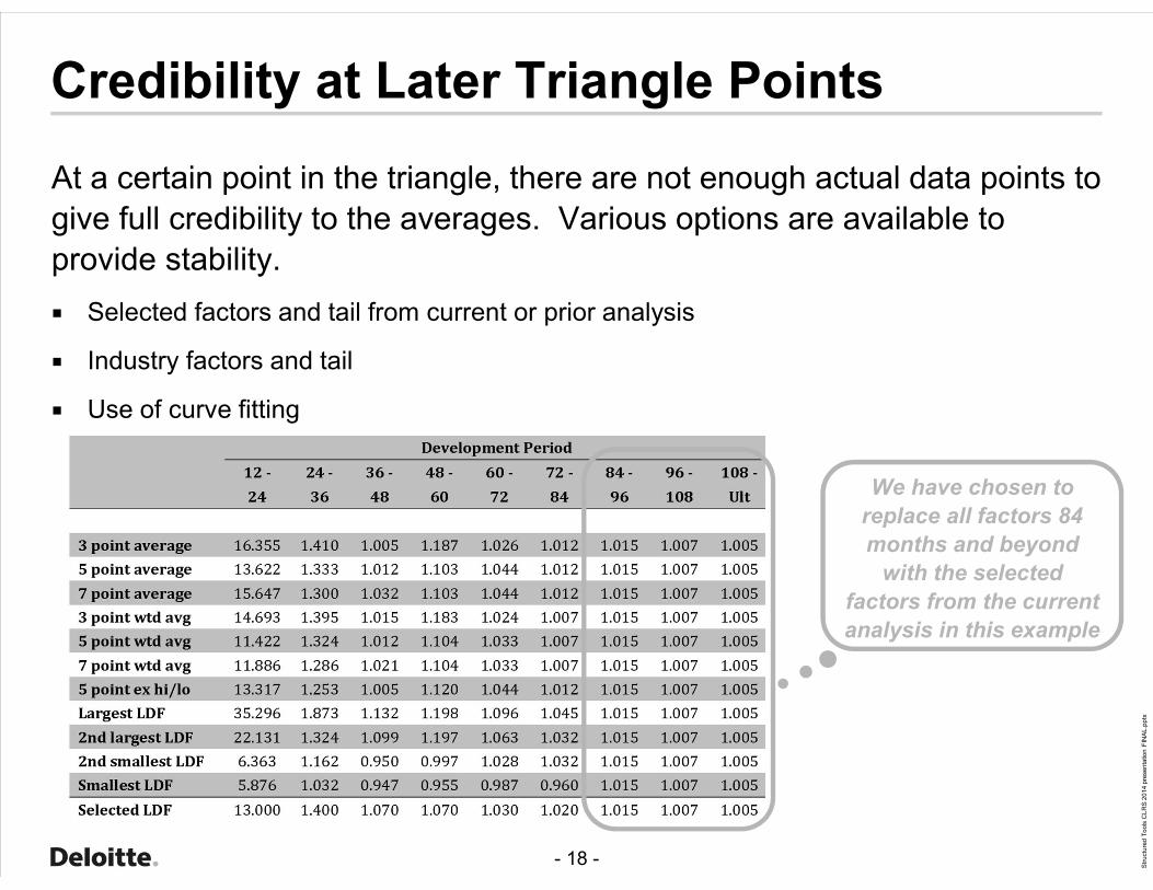
At a certain point in the triangle, there are not enough actual data points to give full credibility to the averages. Various options are available to provide stability.¡ Selected factors and tail from current or prior analysis

¡ Industry factors and tail

¡ Use of curve fitting

Credibility at Later Triangle Points

We have chosen to replace all factors 84months and beyond

with the selected factors from the current analysis in this example

- 19 - Stru

ctur

ed T

ools

CLR

S 20

14 p

rese

ntat

ion

FIN

AL.p

ptx

The next step is to accumulate the factors and calculate the loss development test for each average.

Loss Development Method Calculation

- 20 - Stru

ctur

ed T

ools

CLR

S 20

14 p

rese

ntat

ion

FIN

AL.p

ptx

We total the incurred loss development method results across all accident years for each average and compare this total to the results using the selected LDFs. We have performed the comparison both including and excluding the latest year.

Comparison of Results

We observe that the selected LDFs fall

within the range of the various averages both

including and excluding AY 2012

- 21 - Stru

ctur

ed T

ools

CLR

S 20

14 p

rese

ntat

ion

FIN

AL.p

ptx

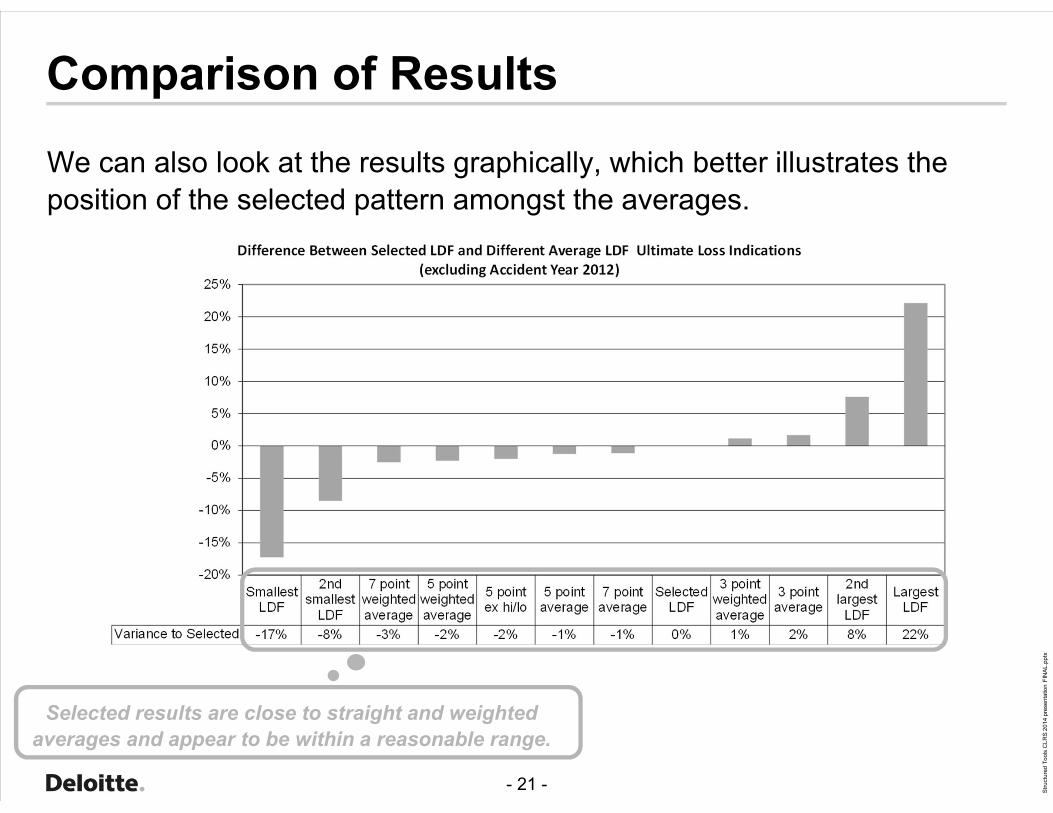
We can also look at the results graphically, which better illustrates the position of the selected pattern amongst the averages.

Comparison of Results

Selected results are close to straight and weighted averages and appear to be within a reasonable range.

- 22 - Stru

ctur

ed T

ools

CLR

S 20

14 p

rese

ntat

ion

FIN

AL.p

ptx

Viewing the different averages may also uncover other trends in the data

Comparison of Results

3 year averages are higher than 5 year and seven year. Are LDFs increasing?

- 23 - Stru

ctur

ed T

ools

CLR

S 20

14 p

rese

ntat

ion

FIN

AL.p

ptx

In this analysis, we examine the drivers of differences between the prior and current ultimate loss selections.

We analyze three drivers:

Source of Change Analysis

¡ Difference between actual and expected loss emergence from the prior analysis to the current analysis

¡ Difference between prior and current assumptions, including loss development factors and initial expected lossesAssumptions

Data

¡ Difference in “Actuarial Judgment” regarding selection of ultimate losses in relation to the ultimate losses indicated by the different actuarial methods

Judgment

- 24 - Stru

ctur

ed T

ools

CLR

S 20

14 p

rese

ntat

ion

FIN

AL.p

ptx

Analyzing these three drivers of change – data, assumptions, and judgment – allows us to comment on the following questions:

¡ What is the impact on ultimate loss estimates of data emerging in a different pattern than expected?

¡ What impact will changing an assumption have on the ultimate loss estimates?

¡ Do any changes in assumptions make sense in relation to what is happening in the data?

¡ Are ultimates selected in a consistent manner relative to the method results? And if not, is this inconsistency reasonable and explainable?

Source of Change Analysis

- 25 - Stru

ctur

ed T

ools

CLR

S 20

14 p

rese

ntat

ion

FIN

AL.p

ptx

We must first calculate three Bornhuetter-Ferguson indications

If exposures are not available, we can follow the same process using the loss development methods, but we have found the BF results to work best due to the stabilizing nature of the methodology that keeps it from over-reacting to large swings in the data.

Source of Change Analysis

¡ BF indication using data as of time t-1 and assumptions as of time t-1

¡ BF indication from prior analysis

¡ BF indication using data as of time t and assumptions as of time t-1

¡ This indication is not calculated or used in either the prior or current analysis

Method B:Current Data

Prior Assumptions

Method A:Prior Data

Prior Assumptions

¡ BF indication using data as of time t and assumptions as of time t

¡ BF indication from current analysis

Method C:Current Data

Current Assumptions

- 26 - Stru

ctur

ed T

ools

CLR

S 20

14 p

rese

ntat

ion

FIN

AL.p

ptx

For this example, we assume time t-1 is 12/31/11 and time t is 12/31/12

BF Method Calculations

(2) * [ 100% - (3) ] + (1)

Method A uses data as of time t-1 and initial

expected loss and LDF assumptions as of time

t-1

- 27 - Stru

ctur

ed T

ools

CLR

S 20

14 p

rese

ntat

ion

FIN

AL.p

ptx

For this example, we assume time t-1 is 12/31/11 and time t is 12/31/12

BF Method Calculations

(2) * [ 100% - (3) ] + (1)

Method B uses data as of time t and initial

expected loss and LDF assumptions as of time

t-1 (interpolated to time t)

- 28 - Stru

ctur

ed T

ools

CLR

S 20

14 p

rese

ntat

ion

FIN

AL.p

ptx

For this example, we assume time t-1 is 12/31/11 and time t is 12/31/12

BF Method Calculations

(2) * [ 100% - (3) ] + (1)

Method C uses data as of time t and initial

expected loss and LDF assumptions as of time t

- 29 - Stru

ctur

ed T

ools

CLR

S 20

14 p

rese

ntat

ion

FIN

AL.p

ptx

The first source of change considered is the change due to data. Unless losses have emerged exactly as expected, updating the loss experience in the analysis will change the resulting method values.

Change due to data should be similar to the indirect actual vs. expected results. However, this test goes one step further to tell us how much the change in data is impacting our method indications.

Change due to Data

Method B

10,984

Method A

10,713

Change due to Data

272

The results show that the data has emerged higher than expected. An increase in the method results due to a change in data indicates that

either the assumptions underlying the prior analysis projected too little development in the period or that the ultimate losses from the prior

analysis should be increased (or some combination of the two)

- 30 - Stru

ctur

ed T

ools

CLR

S 20

14 p

rese

ntat

ion

FIN

AL.p

ptx

The second source of change considered is the change due to assumptions – in this case loss development factors and initial expected losses. Additional insight from having another year’s worth of data may lead us to change our assumptions.

Method B

10,984

Method C

10,935

Change due to Assumptions

Change due to Assumptions

(49)

The results show that the assumptions in the current analysis are lower than the assumptions in the prior analysis.

- 31 - Stru

ctur

ed T

ools

CLR

S 20

14 p

rese

ntat

ion

FIN

AL.p

ptx

For methods with multiple assumptions, we can break out the change in assumptions to measure the change due to each individual assumption, if desired. To do so, calculate successive method values changing one assumption at a time.

Change due to Assumptions – Detailed

Method B1¡ BF indication using current data and all prior assumptions

Method B2

Method B3

Method C

¡ BF indication using current data, current age to age factors, prior tail factor (interpolated to current age), and prior initial expected losses

¡ BF indication using current data, current age to age factors, current tail factor, and prior initial expected losses

¡ BF indication using current data and all current assumptions

- 32 - Stru

ctur

ed T

ools

CLR

S 20

14 p

rese

ntat

ion

FIN

AL.p

ptx

With these methods, we can break the change in assumptions down into its component parts.

Change due to Assumptions – Detailed

Method B1Method B2

Method B3

Method C

Change due to Age to Age Factors

Change due to Tail FactorMethod B2

Change due to Initial Expected LossMethod B3

- 33 - Stru

ctur

ed T

ools

CLR

S 20

14 p

rese

ntat

ion

FIN

AL.p

ptx

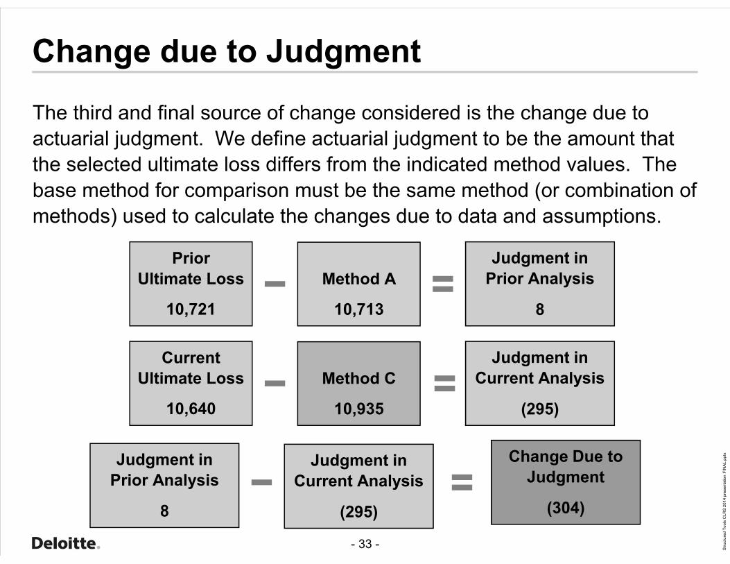
The third and final source of change considered is the change due to actuarial judgment. We define actuarial judgment to be the amount that the selected ultimate loss differs from the indicated method values. The base method for comparison must be the same method (or combination of methods) used to calculate the changes due to data and assumptions.

Judgment in Prior Analysis

8

Prior Ultimate Loss

10,721

Method A

10,713

Change due to Judgment

Judgment in Current Analysis

(295)

CurrentUltimate Loss

10,640

Method C

10,935

Judgment in Prior Analysis

8

Judgment in Current Analysis

(295)

Change Due to Judgment

(304)

- 34 - Stru

ctur

ed T

ools

CLR

S 20

14 p

rese

ntat

ion

FIN

AL.p

ptx

We can also demonstrate that the change due to judgment is equal to the remaining change in ultimates that is not accounted for in the change due to data or the change due to assumptions.

Change due to Judgment

Judgment in Prior Analysis

8

Judgment in Current Analysis

(295)

Change Due to Judgment

(304)

Change in Ultimate Loss

(81)

Prior Ultimate Loss

10,721

CurrentUltimate Loss

10,640

Change due to Data

272

Change in Ultimate Loss

(81)

Change due to Assumptions

(49)

Change Due to Judgment

(304)

- 35 - Stru

ctur

ed T

ools

CLR

S 20

14 p

rese

ntat

ion

FIN

AL.p

ptx

We have found it beneficial to view the Source of Change results graphically.

Source of Change – Interpreting Results

The graph shows us that while data has emerged higher than expected, the actuary is lowering LDF assumptions and judgment in the current analysis.

This may lead us to ask why?

- 36 - Stru

ctur

ed T

ools

CLR

S 20

14 p

rese

ntat

ion

FIN

AL.p

ptx

It can be helpful to break the changes down into smaller steps. We can look at the assumptions separately, as discussed earlier, or look at the component changes for each accident year to see if there is one year driving the results.

Source of Change – Interpreting Results

In our example, we see that accident year 2011 is driving the results due to data. After excluding accident year

2011 from the calculation, the decreases in assumptions and

judgment make more sense

- 37 - Stru

ctur

ed T

ools

CLR

S 20

14 p

rese

ntat

ion

FIN

AL.p

ptx

¡ Do I worry if the change due to data is inconsistent with the actual vs. expected results?

¡ Do I worry if I see different directional changes in my LDF picks and my IELR?

¡ Do I worry if I see a large judgment impact?

Discussion Questions

- 38 - Stru

ctur

ed T

ools

CLR

S 20

14 p

rese

ntat

ion

FIN

AL.p

ptx

¡ Methodology is not designed to provide answers, but rather a structured framework through which to examine a reserve analysis.

¡ Methodology is designed to lead the actuary to ask questions that lead to a better understanding of the results of the actuarial analysis.

¡ Can be a valuable tool in teaching less experienced practitioners the type of critical thinking needed when performing a reserve analysis.

¡ Source of change results over multiple years can be used to evaluate trends in the analysis over time.

Conclusions

Copyright © 2012 Deloitte Development LLC. All rights reserved.