ClickHere

for

FullArticle

Structure of magnetic separators and separator reconnection

C. E. Parnell,1 A. L. Haynes,1 and K. Galsgaard2

Received 12 June 2009; revised 2 August 2009; accepted 11 September 2009; published 26 February 2010.

[1] Magnetic separators are important locations of three‐dimensional magneticreconnection. They are field lines that lie along the edges of four flux domains andrepresent the intersection of two separatrix surfaces. Since the intersection of two surfacesproduces an X‐type structure, when viewed along the line of intersection, the global three‐dimensional topology of the magnetic field around a separator is hyperbolic. It is thereforeusually assumed that the projection of the magnetic field lines themselves onto a two‐dimensional plane perpendicular to a separator is also hyperbolic in nature. In this paper,we use the results of a three‐dimensional MHD experiment of separator reconnection toshow that, in fact, the projection of the magnetic field lines in a cut perpendicular to aseparator may be either hyperbolic or elliptic and that the structure of the magnetic fieldprojection may change in space, along the separator, as well as in time, during the life ofthe separator. Furthermore, in our experiment, we find that there are both spatial andtemporal variations in the parallel component of current (and electric field) along theseparator, with all high parallel current regions (which are associated with reconnection)occurring between counterrotating flow regions. Importantly, reconnection occurs not onlyat locations where the structure of the projected perpendicular magnetic field is hyperbolicbut also where it is elliptic.

Citation: Parnell, C. E., A. L. Haynes, and K. Galsgaard (2010), Structure of magnetic separators and separator reconnection,J. Geophys. Res., 115, A02102, doi:10.1029/2009JA014557.

1. Introduction

[2] Magnetic reconnection is a fundamental plasma phys-ics process that plays an important role in many solar, mag-netospheric, and astrophysical phenomena. Realistic modelingof all these reconnection environments must be done in threedimensions, not simply because they are three dimensional,but, more importantly, because 3‐D reconnection is funda-mentally different than 2‐D reconnection.[3] In two dimensions, magnetic reconnection can only

occur at X‐type null points. At the null a pair of field lineswith different connectivities, say, A → A′ and B → B′, arereconnected to form a new pair of field lines with connec-tivities A → B′ and B → A′. Hence, flux is transferred fromone pair of flux domains into another pair of flux domains.Furthermore, in two dimensions, reconnection involves anX‐type stagnation flow and results in a discontinuous jumpin the field line mapping at the instant reconnection takesplace. There has been a considerable body of work on 2‐Dreconnection, and extensive reviews can be found, forexample, in the works by Priest and Forbes [2000] andBiskamp [2000].

[4] The early research into the nature of 3‐D reconnectionnaturally evolved from the 2‐D reconnection work, andvarious definitions of 3‐D reconnection were proposed,including “plasma flows across a surface which separatesregions including topologically different magnetic fieldlines” [Vasyliunas, 1975, p. 304], “presence of an electricfield along a separator” [Sonnerup, 1979, p. 879], “transferof plasma‐elements from one field line to another (i.e., abreak down of the frozen‐in flux theorem)” [Axford, 1984,p. 1], and “evolution in which it is not possible to preservethe global identification of some field lines” (i.e., magneticfield evolution that is not flux preserving) [Greene, 1993,p. 2355]. The first two of these definitions require theexistence of 3‐D magnetic nulls in order to produce themagnetic separatrices and separators which are an essentialpart of these reconnection scenarios. However, Schindler etal. [1988] and Hesse and Schindler [1988] proposed atheory of generalized magnetic reconnection in which theyestablished that 3‐D reconnection does not require nulls orstructures associated with nulls and which encompasses thereconnection definitions previously suggested. In particu-lar, 3‐Dmagnetic reconnection occurs not only at 3‐D nulls[e.g., Craig et al., 1995; Craig and Fabling, 1996; Priestand Titov, 1996; Pontin and Craig, 2005; Pontin andGalsgaard, 2007; Pontin et al., 2007a, 2007b], but morecommonly it occurs in a null‐less region of a magnetic field[Schindler et al., 1988; Hesse and Schindler, 1988], forinstance, in a hyperbolic flux tube [Priest and Démoulin,1995; Démoulin et al., 1996; Titov et al., 2003; Galsgaard

1School of Mathematics and Statistics, University of St. Andrews,Saint Andrews, UK.

2Niels Bohr Institute, Copenhagen, Denmark.

Copyright 2010 by the American Geophysical Union.0148‐0227/10/2009JA014557$09.00

JOURNAL OF GEOPHYSICAL RESEARCH, VOL. 115, A02102, doi:10.1029/2009JA014557, 2010

A02102 1 of 10

et al., 2003; Linton and Priest, 2003; Aulanier et al., 2005;Pontin et al., 2005a; Aulanier et al., 2006; De Moortel andGalsgaard, 2006a, 2006b; Wilmot‐Smith and De Moortel,2007] or at mode‐rational surfaces [Browning et al., 2008;Hood et al., 2009]. Also, recently, Titov et al. [2009] haveproposed a general method for determining the magneticreconnection in arbitrary 3‐D magnetic configurations. Theydemonstrate, using their method, that, along with magneticnull points, hyperbolic and cusp minimum points are alsofavorable sites for magnetic reconnection.[5] We are concerned in this paper with separator recon-

nection, and since separators link pairs of opposite‐polaritynull points, reconnection at a separator has been viewed bymany as reconnection involving null points. Separators andseparator reconnection have been considered by various au-thors [e.g., Sonnerup, 1979; Lau and Finn, 1990; Longcopeand Cowley, 1996; Galsgaard and Nordlund, 1997;Galsgaard et al., 2000b; Longcope, 2001; Pontin and Craig,2006; Haynes et al., 2007; Parnell et al., 2008; Dorelli andBhattacharjee, 2008]. The authors are unaware of anypapers that specifically address the importance of the nullsduring separator reconnection; this is one of the questions thatis addressed in this paper.[6] Many, but not all, of the above situations depend on

the fact that field lines from flux domains with two differentconnectivities, say, A → A′ and B → B′, are reconnected toform field lines in two new flux domains with connectivitiesA → B′ and B → A′, exactly as in the 2‐D case. In threedimensions, however, it is generally not possible to identifypairs of field lines that reconnect to form new pairs of fieldlines [e.g., Hornig and Priest, 2003; Pontin et al., 2005b],apart from nongeneric special cases. Instead, reconnectionwill occur continually and continuously throughout thefinite diffusion region, converting flux from two domainsinto flux in two other domains. A consequence of this isthat, in three dimensions, the field line mapping is, in general,continuous between prereconnected and postreconnectedfield lines, as opposed to discontinuous. The theory behindthis behavior is explained by Hornig and Priest [2003] usinga kinematic model and is illustrated very nicely usingnumerical experiments by Pontin et al. [2005a] and Aulanieret al. [2006]. From their kinematic model, Hornig and Priest[2003] hypothesize that counterrotating flows are an impor-tant ingredient of 3‐D reconnection. Also, note that such aflow pattern is implicit within the general reconnection modelof Hesse [1995].[7] Generic magnetic separators are lines which divide

four topologically distinct flux domains and hence are loca-tions about which reconnection often occurs. They are theintersection of two separatrix surfaces. (Nongeneric separa-tors involve a spine line from a null, but we ignore these sincethey are structurally unstable.) Separatrix surfaces are sur-faces of field lines that encompass flux from a single source.The field lines in these surfaces originate from nulls, baldedges [Haynes, 2007], or bald patches [Bungey et al., 1996].The four flux domains surrounding a separator are divided bythe two separatrix surfaces. Separators are often termed“X lines” because of the belief that the projection of themagnetic field lines in a 2‐D plane perpendicular to theseparator has the form of a 2‐DX point. Note, however, thatthe term X line is ambiguous and is also commonly used

for a line of X‐type nulls, which is a structurally unstabletopological feature [e.g., Hesse and Schindler, 1988]. Wetherefore do not adopt this term.[8] The aim of this paper is to determine the main char-

acteristics of separator reconnection. In order to make thework in this paper clear, we first explain our terminology insection 2. For comparative purposes, we then discuss brieflythe magnetic field of potential separators (section 3). Ourmain interest is in investigating the 3‐D magnetic fieldstructure of nonpotential separators and, during separatorreconnection, the relationship between the magnetic andvelocity fields in 2‐D planes perpendicular to the separator.To do this, we use a 3‐D resistive MHD experiment whichis described in section 4. In section 5, we address the fol-lowing questions: (1) What is the nature of the currentdensity along a separator? (2) Where does reconnectionoccur along separators? (3) What is the projection of the 3‐Dmagnetic field in a 2‐D cut perpendicular to a separator?(4) During reconnection, what is the structure of the 3‐Dvelocity field in the vicinity of a separator? Finally, theconclusions drawn from our results are discussed insection 6.

2. Terminology

[9] In this paper, we investigate the 3‐D magnetic and3‐D velocity field structures about separators. Since it isnot easy to visualize 3‐D magnetic fields in still images,we consider projections of the magnetic field in 2‐D planes.In general, such projections can be misleading since theresults will differ for each orientation of the projectionplane. Thus, to analyze the 3‐D magnetic field about aseparator at a given point along it, we project the magneticfield onto the unique 2‐D plane which is perpendicular tothe separator at that point. Thus, we can reliably investigatethe 3‐Dmagnetic field both along the length of the separatorand also as the separator varies in times. Before we discussour work, we first define a few terms.[10] 1. The 3‐D topology of a magnetic field is outlined

by its magnetic skeleton, which is made up of sources, nulls,separatrix surfaces, and separators. Therefore, the 3‐Dtopological structure is a global phenomenon. Note thathere we use the word global to mean “large scale” in ageneral sense and not as a reference to the whole Sun ormagnetosphere.[11] 2. The 3‐D magnetic field structure is defined by the

behavior of the magnetic field lines and hence is a local (i.e.,“small‐scale”) phenomena. The structure may be defined ashyperbolic or elliptic depending on the structure of the 2‐Dprojected field in a perpendicular cross section through themagnetic field: a 2‐D saddle (X) or improper fixed point isseen if the 3‐D magnetic field structure is hyperbolic, anda 2‐D spiral or ellipse (O) is seen if the field structure iselliptic (i.e., has a 3‐D helical‐type structure).[12] 3. The 2‐D projected field is the projection of the

magnetic field in planes perpendicular to the separator. LetB be any 3‐D magnetic field that contains a separator andlet x0 be a point on the separator with nk(x0) as the vectordirected along the separator at this point. Then the com-ponent of the magnetic field parallel to the separator at x0

PARNELL ET AL.: SEPARATORS AND SEPARATOR RECONNECTION A02102A02102

2 of 10

is given by Bkx0 = [B · nk(x0)]nk(x0), and therefore, theperpendicular magnetic field component is

B?x0 ¼ B� Bkx0 : ð1Þ

The 2‐D projection of the magnetic field in the planeperpendicular to the separator at x0 is defined as B?x0evaluated in that plane. We call this 2‐D projected fieldProjB?x0. Note that the 2‐D projected field is not amagnetic field since it does not satisfy the solenoidalconstraint, as shown in section 3. The 2‐D projected fieldstructure can be defined as hyperbolic or elliptic, using thepreviously described definitions, depending on the natureof the fixed point in the 2‐D projected field where theseparator pierces the perpendicular 2‐D plane.[13] In purely 2‐D magnetic fields, the magnetic topology

and magnetic field line structure coincide, and hence, the2‐D global and local magnetic structures are the same. It isnot possible to determine the global magnetic topology ofa 3‐D magnetic field unless you know the magnetic fieldin a large number of locations, which is obviously not thecase from solar and magnetospheric observations. Instead,estimations of the local 3‐D magnetic field and 2‐D pro-jections of the magnetic field have been made in magne-tospheric physics. In solar physics, images of the solaratmosphere reveal some structure of the magnetic field, asdo extrapolations of the local 3‐D magnetic field above thephotosphere. Here we show that, unlike in two dimen-sions, the 3‐D magnetic topology and local 3‐D magneticfield line structure are not the same. Therefore, in order tohelp with the interpretation of observational (and numer-ical) results, we investigate what local 3‐D magneticfield and 2‐D projected field structures are associated withseparators.

3. Magnetic Field of a Potential Separator

[14] The 3‐D magnetic topology in the vicinity of a sep-arator (potential or nonpotential) is given by the separatrixsurfaces that intersect to form the separator. As mentioned insection 2, a cut perpendicular to the separator reveals thatthe two separatrix surfaces form an “X,” so we describe the

global 3‐D magnetic topology in the vicinity of a separatoras being hyperbolic (Figure 1a).[15] In the vicinity of a potential separator, what is the

local 3‐D magnetic field structure? To answer this question,we need to consider the 2‐D projected field structure inplanes perpendicular to the separator. By definition, both thedivergence and curl of a potential magnetic field are zero,but what are the divergence and curl of the 2‐D projectedfield in cuts perpendicular to the separator?[16] Let us consider, without loss of generality, a mag-

netic field, Bpot = (Bpx, Bpy, Bpz), which has a pair of 3‐Dnulls at points (0, 0, a) and (0, 0, b) orientated such that theirseparatrix surfaces intersect along the z axis and a separatorlies along this line between z = a and z = b. Hence, Bpot?(x,y, z) = (Bpx, Bpy, 0) and Bpotk(x, y, z) = (0, 0, Bpz). For anypoint (0, 0, z0) along the separator, where a < z0 < b, the 2‐Dprojected perpendicular field is ProjBpot?z0(x, y) = Bpot?(x,y, z0); hence, its components are functions of x and y but notz. Thus, the divergence of the 2‐D projected field becomes

r � ProjBpot?z0ðx; yÞ ¼ @Bpxðx; y; z0Þ@x

þ @Bpyðx; y; z0Þ@y

6¼ 0

since

@Bpzðx; y; zÞ@z

����z¼z0

6¼ 0:

Therefore ProjBpot?z0 is not a magnetic field, but simply a2‐D vector field. Now, the curl of ProjBpot?z0(x, y) is

r� ProjBpot?z0ðx; yÞ ¼ 0; 0;@Bpyðx; y; z0Þ

@x� @Bpxðx; y; z0Þ

@y

� �

¼ ð0; 0; 0Þ

since the 3‐D magnetic field is potential. We note here thatthe curl of the projected magnetic field and the projection ofthe curl of the magnetic field are not commutative, andhence the result above is true for potential fields.[17] Thus, in general, if one linearized ProjBpot?z0(x, y)

about the point (0, 0) through which the separator piercesthe plane, the magnetic field would have the form

ProjBpot?z0ðx; yÞ �a c=2c=2 b

� �xy

� �: ð2Þ

The eigenvalues of this field are

�� ¼ aþ b

2� 1

2

ffiffiffiffiffiffiffiffiffiffiffiffiffiffiffiffiffiffiffiffiffiffiffiffiffiffiffiða� bÞ2 þ c2

q;

so they are always real. This means the structure of the local2‐D projected field in a plane perpendicular to a potentialseparator can be either an X point, a stable or unstableproper node (star), or a stable or unstable improper nodedepending on the relative values of a, b, and c.[18] Now, if the 2‐D plane perpendicular to the separator

is at either of the 3‐D nulls at the ends of the separator, theX‐type 2‐D projected field structure will coincide with theX‐type structure formed by the 3‐D separatrix surfaces. Ithas long been believed that this holds true along the com-

Figure 1. (a) The intersection of the two separatrix surfaces(shown in blue and pink) indicates the X‐type nature of theglobal 3‐D topology about a separator (thick yellow line).(b) The 2‐D projected field structure in a plane perpendicu-lar to the separator (white lines on grey plane) has a nullpoint which coincides with the point at which the separatorpierces the plane. The X‐type structure of the 2‐D projectedfield does not coincide with the 3‐D global X‐type structureformed by the intersection of the two separatrix surfaces.

PARNELL ET AL.: SEPARATORS AND SEPARATOR RECONNECTION A02102A02102

3 of 10

plete length of the separator; however, as we have justshown, this is not necessarily the case since, for some por-tion of the separator, the projection of the 2‐D perpendicularfield may look like a star or an improper fixed point. Fur-thermore, the two separatrix surfaces forming the separatordo not necessarily intersect at right angles along the com-plete length of the separator, so the global 3‐D topologydoes not necessarily form a right‐angled “X.” However, ifthe 2‐D projected field structure is a saddle, then this Xstructure must be right angled since r × ProjBpot? = 0.Thus, these two X‐type structures cannot always coincide,as shown in Figure 1b. Therefore, the 2‐D projected fieldstructure in a plane perpendicular to the separator does notnecessarily reflect the global 3‐D magnetic topology of thefield. Hence, the local 3‐D magnetic field structure andglobal 3‐D magnetic topology do not necessarily coincideeither.[19] In light of this rather surprising discovery about the

nature of the local 3‐Dmagnetic field structure in the vicinityof a potential separator, we now go on to consider non-potential separators and separator reconnection. To do this,we use results from a numerical experiment which we brieflyreview as a whole in section 4 before focusing on the detailsof the separators in this experiment in section 5.

4. Three‐Dimensional Numerical Model

[20] The 3‐D numerical setup used here is very similar tothat used by Galsgaard et al. [2000a], Haynes et al. [2007],

Parnell et al. [2008], and A. L. Haynes et al. (The effects ofmagnetic resistivity on a magnetic flyby model, manuscriptin preparation, 2010), so we only give a very brief de-scription here. We consider a Cartesian grid of 256 × 256 ×129 scaled to 1 × 1 × 1/4. The initial magnetic field is po-tential and involves two sources of finite extent on the baseof the box which contain equal amounts of flux but are ofopposite polarity. An overlying field is then added in the ydirection to ensure that the sources are initially discon-nected. The side boundaries of the box are periodic, whilethe top boundary is closed. On the base, the boundary isclosed apart from the two sources. The sources are drivenalong lanes, at a speed of 0.02 of the initial peak Alfvénspeed in the box, such that they run antiparallel to each otherin a direction perpendicular to the overlying field (the xdirection), resulting in the interaction of their fluxes by wayof reconnection at a series of separators. The drivers areswitched off before the sources leave the box at 26.7 Alfvéncrossing times (where the crossing time of the box is de-termined from the peak Alfvén speed). We start with auniform atmosphere which has an initial density and pres-sure of 1/4 and 1/6, respectively, in dimensionless units.[21] The numerical code is a resistive MHD code which

has a staggered grid and uses sixth‐order spatial derivativeswith fifth‐order interpolation. Time is advanced by a third‐order predictor‐corrector method. In this paper, we consideran experiment in which the magnetic resistivity is heldconstant at 6.25 × 10−5. The Lundquist number for theexperiment is 18,693 (determined from the same values asthe Alfvén crossing time). However, the local magnetic

Figure 2. Snapshots showing the nonpotential magnetic skeleton of our model at times (a) t = 2.53, (b) t =4.50, (c) t = 13.47, and (d) t = 17.85, including the positive and negative sources on the base (white and blackdiscs), the positive and negative separatrix surfaces (pink and blue surfaces), and separators (thick yellowlines).

PARNELL ET AL.: SEPARATORS AND SEPARATOR RECONNECTION A02102A02102

4 of 10

Reynolds number within our domain can vary greatly fromorder unity up to several thousand.

5. Separators and Separator Reconnection

[22] The magnetic configuration in our experiment involvestwo magnetic nulls on the base of the box which remain forthe entire experiment. The initial setup is shown in Figure 2aand contains no separators. However, the boundary drivingmotions lead to the creation of a number of separators linkingthe two nulls, as described by Haynes et al. [2007]. In par-ticular, the first separators created are a pair formed by aglobal double‐separator bifurcation, as shown in Figure 2b.The lower of these two separators rapidly disappears at thebase of the box, leaving the upper separator, which lasts formost of the experiment. This separator is visible in Figures 2cand 2d (central separator). It is this separator that we inves-tigate in detail. Further separators are formed (Figure 2d),but since their characteristics are similar to the one we arefocusing on we do not discuss them in detail.

5.1. Nature of the Current Along a ReconnectingSeparator

[23] In separator reconnection the rate of reconnection isrelated to the amount of electric field parallel to the sepa-rator [Sonnerup, 1979; Hesse and Birn, 1993; Hesse, 1995;Parnell et al., 2008]. When the resistivity h is constant, theparallel electric field is simply related to the parallel electriccurrent by a factor h. Thus, studying the nature of the par-allel current along the separator reveals where, along thelength of the separator, reconnection is actually occurring.[24] Figure 3a shows a contour plot of the parallel current

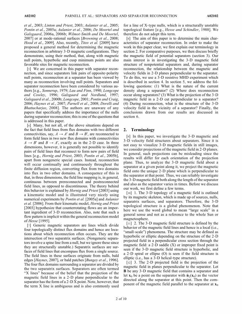
along the length of the separator varying in time. Clearly,the current (and hence the reconnection) is neither constant

in time nor constant along the length of the separator. Ini-tially (t = 4.78), the current grows from two locations nearthe ends of the separator but not at the nulls (Figure 3b). Thecurrent then spreads out along the separator and increases inintensity. At about 14.03 Alfvén times the current peaksnear the center of the separator. Later on (during a phaseincluding further separators) the currents are seen to have adouble (t = 25.74) and triple (t = 28.16) peaked nature(Figure 3b).

5.2. Where Does Reconnection Occur AlongSeparators?

[25] The reconnection along the separator occurs wherethere are high parallel currents and, hence, high parallelelectric fields. From our analysis it is clear that separatorreconnection does not (only) occur at the nulls at the ends ofthe separator but that the vast majority occurs in one or morelocalized regions along its length. In our experiment thereare periods with what appear to be two or three enhancedregions of reconnection along a single separator, as well asperiods where there is just one site extending over much ofthe length of the separator (Figure 3).[26] The reconnection rate rsep at the separator is given by

the formula [Hesse and Birn, 1993; Hesse, 1995; Hornigand Priest, 2003; Parnell et al., 2008]

rsep ¼ d�

dt¼

ZlEkdl ¼ �

Zljkdl; ð3Þ

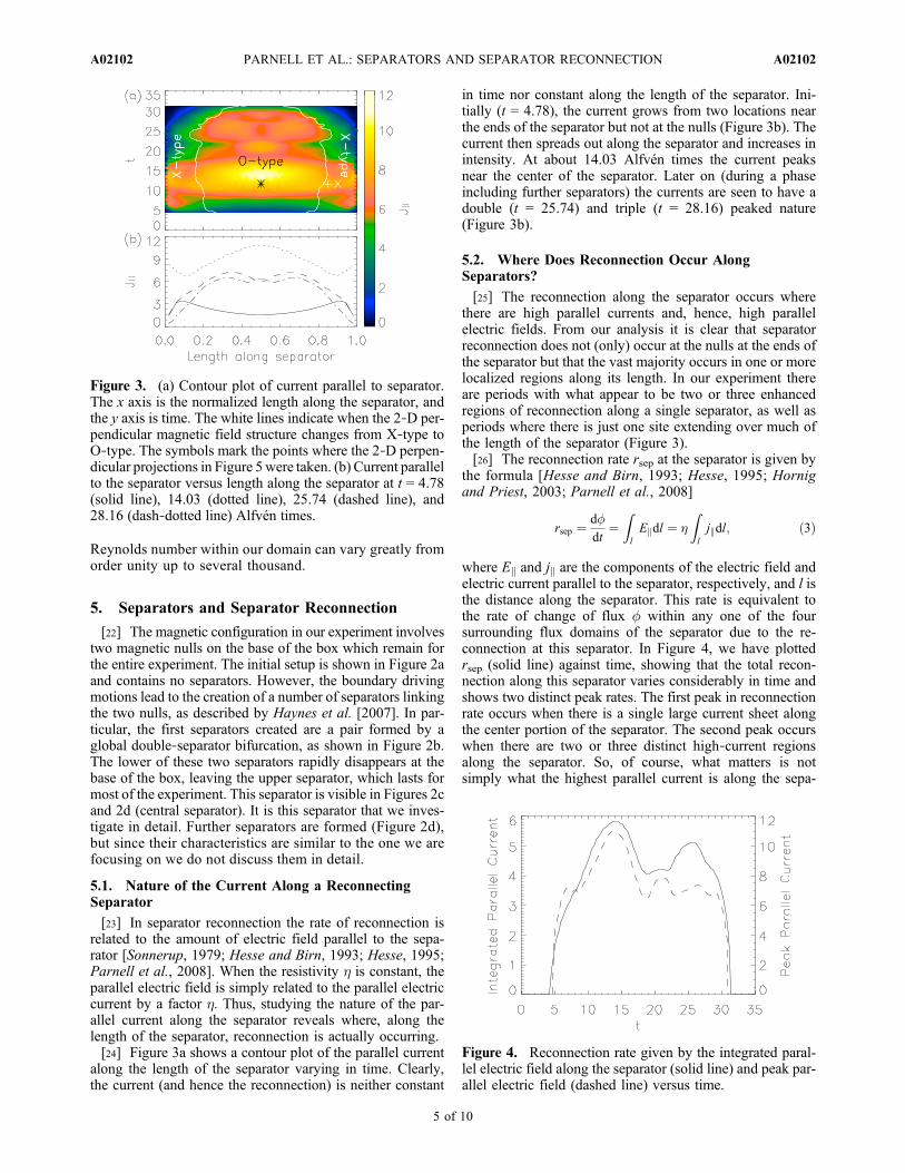
where Ek and jk are the components of the electric field andelectric current parallel to the separator, respectively, and l isthe distance along the separator. This rate is equivalent tothe rate of change of flux � within any one of the foursurrounding flux domains of the separator due to the re-connection at this separator. In Figure 4, we have plottedrsep (solid line) against time, showing that the total recon-nection along this separator varies considerably in time andshows two distinct peak rates. The first peak in reconnectionrate occurs when there is a single large current sheet alongthe center portion of the separator. The second peak occurswhen there are two or three distinct high‐current regionsalong the separator. So, of course, what matters is notsimply what the highest parallel current is along the sepa-

Figure 3. (a) Contour plot of current parallel to separator.The x axis is the normalized length along the separator, andthe y axis is time. The white lines indicate when the 2‐D per-pendicular magnetic field structure changes from X‐type toO‐type. The symbols mark the points where the 2‐D perpen-dicular projections in Figure 5 were taken. (b) Current parallelto the separator versus length along the separator at t = 4.78(solid line), 14.03 (dotted line), 25.74 (dashed line), and28.16 (dash‐dotted line) Alfvén times.

Figure 4. Reconnection rate given by the integrated paral-lel electric field along the separator (solid line) and peak par-allel electric field (dashed line) versus time.

PARNELL ET AL.: SEPARATORS AND SEPARATOR RECONNECTION A02102A02102

5 of 10

rator (dashed line in Figure 4) but the extent of the region(s)over which the parallel current is high (i.e., the size of theoverall reconnection site).

5.3. Projected 3‐D Magnetic Field in a 2‐D CutPerpendicular to the Separator

[27] We have already seen in section 2 that for potentialfields, the global 3‐D magnetic topology and local 3‐Dmagnetic field structures do not necessarily coincide. Herewe consider what the local 3‐D magnetic field structure isabout a nonpotential separator by looking at ProjB?, the2‐D projected field perpendicular to it.[28] The magnetic field in the vicinity of a separator

typically has a strong component parallel to the direction ofthe separator, although this is not true near the ends of theseparator. Again, we use equation (1) to determine the 2‐Dprojected field in a plane perpendicular to the separator, andwe recall that this 2‐D field has a null at the point where theseparator pierces the plane.[29] We have already found that the 2‐D projected field

structure in a plane perpendicular to a potential separator canbe an X‐type or a proper or improper node since the linearfield always has real eigenvalues. In the nonpotential case,though, there are likely to be currents parallel to the sepa-rator as there are during separator reconnection. We find,using the same notation as equation (2), that, to first order,the 2‐D projected field ProjB? about the 2‐D null point at

which the separator pierces the plane, located at the originfor simplicity, has the form

ProjB? ¼ a ðc� jkÞ=2ðcþ jkÞ=2 b

� �x1x2

� �; ð4Þ

where x1 and x2 are orthogonal coordinates lying in the 2‐Dperpendicular plane. The 2‐D null will have real eigenvaluesif (a − b)2 + c2 > jk

2 (creating an X point or a proper orimproper node), and the field will have complex eigenvaluesif (a − b)2 + c2 < jk

2 (creating a spiral or O‐type node), wherejk is the component of current out of the plane. Hence, linear2‐D projected fields are typically spiral or O‐type if thecurrent is large (relative to the other components in thematrix). Therefore, ProjB? about a nonpotential separatorcould take on one of many forms, and its structure is likelyto vary along the separator.[30] Plots of ProjB? determined at 1/2 (Figure 5a) and

9/10 (Figure 5b) of the way along the separator at t = 13.47reveal that, indeed, the 2‐D projected field structure per-pendicular to our separator does change in nature along thelength of the separator. ProjB? is of O type near the centerof the separator while it appears to be of X type near itsend. The asterisk and plus in Figure 3 indicate the pointswhere the above two 2‐D perpendicular plots were taken.We determined the nature of ProjB? at every point alongour separator for every time step and overplotted white

Figure 5. Plots showing (top) the 2‐D projected field structure (white lines) and (bottom) the 2‐D ve-locity field structure (white lines) in perpendicular planes at (a) 0.5, (b) 0.9, (c) 0.5, and (d) 0.85 along theseparator at time t = 13.47. The separator (thick line coming out of the plane) is shaded according to itsparallel current (current, red; temperature (low and high), black and white). The contours on the surfaceperpendicular to the separator show the absolute current in the plane (Figures 5a and 5b) (low (black) tohigh (red)) and the radial velocity in the plane with respect to the point at which the separator pierces theplane (Figures 5c and 5d) (inflow, blue and green; outflow, red and yellow).

PARNELL ET AL.: SEPARATORS AND SEPARATOR RECONNECTION A02102A02102

6 of 10

lines in Figure 3 where the nature of ProjB? changes.These lines reveal that for the entire life of our separator itsperpendicular 2‐D projected field structure has real eigen-values (e.g., is of X type) near the ends of the separator andhas complex eigenvalues (e.g., is either spiral or O‐type) inthe middle, although the length of this complex eigenvalueregion changes in time (note that the other two long‐livedseparators in our experiment show a similar pattern forProjB?). Indeed, for all generic separators (separatorscreated by the intersection of two separatrix surfaces) whichhave a null at either end, ProjB? must have an X‐typenature at the ends of the separator, so it is not a surprise thatour separators show this feature. The spiral or O‐type naturein the middle can be explained by the fact that our two se-paratrix surfaces are driven such that they entwine aroundeach other even though our driving flow is just a simpleshear flow. Thus, even though the global 3‐D topology ofthe magnetic field near the separator is always X‐type, thelocal 3‐Dmagnetic field structure about the separator can beeither hyperbolic or elliptic along different regions of thesame separator. Also, the local 3‐D field structure canchange its nature in time.

5.4. Structure of the 3‐D Velocity About aReconnecting Separator

[31] The specific locations along the separator that havehigh currents should be the locations where the flux isreconnecting fastest. From Figure 3, it can be seen thatthese locations do not coincide exclusively with spiral orO‐type perpendicular fields; however, many of them do.Thus, hyperbolic local 3‐D magnetic field structures arenot essential for reconnection: elliptic ones are also pos-

sible reconnection sites. Therefore, knowing the local 3‐Dstructure of a magnetic field does not allow us to identify aseparator or separator reconnection, but is there anythingspecial about the local 3‐D velocity structure that can allowus to identify possible separator reconnection?[32] From the induction equation, which describes the rate

of change of the magnetic field, one can see that recon-nection requires not only high currents to produce a diffu-sion region but also a velocity flow that carries the magneticfield through the ideal region into the diffusion region. Thus,we also consider what the nature of the 2‐D projected ve-locity structure perpendicular to the separator is, whereProjv? is equal to v? evaluated in the perpendicular planeand v? = v − (v · nk)nk. In Figures 5c and 5d, we show twoplots of Projv? (lines) relative to the separator taken at thesame time as the two graphs in Figures 5a and 5b. InFigure 5c, where the parallel current (hence parallel electricfield) is high (indicated by the asterisk in Figure 3), and thusreconnection is strong, the projection of the streamlinesonto this plane reveals an X‐type stagnation flow within theimmediate vicinity of the separator. However, where re-connection is slower (i.e., the parallel current and electricfield are low, as indicated by the cross in Figure 3), we havean O‐type stagnation flow (Figure 5d). The contours inFigures 5c and 5d reveal the radial flow from the separatorin the plane and show that both flows can give rise to dis-tinct narrow outflow jets associated with the reconnection.[33] The blue and green filled contours in Figure 6a

indicate on a time‐distance graph where the 2‐D perpen-dicular velocity structure has complex eigenvalues (spiralor O type), and the red and yellow filled contours indicatewhere they are real (improper or X type). In comparisonwith Ek (contour lines in Figure 6a) the 2‐D perpendicularvelocity structure is of improper or X type in the regionswhere the electric field is largest. However, the 2‐D per-pendicular velocity structure is not of improper or X typealong the complete length of the separator. This seems toimply that for 3‐D reconnection it is not essential to have a2‐D perpendicular X‐type stagnation flow; instead, a 2‐Dperpendicular spiral or O‐type stagnation flow is possible.[34] Thus, we consider what other characteristic of the

velocity may be important for reconnection. In particular,following Hornig and Priest [2003], we look for counter-rotating flows on either side of the main reconnection region.Figure 6b shows a contour plot of (r × Projv?) · nk. Red andyellow indicate (r × Projv?) · nk > 0, and green and blueindicate (r × Projv?) · nk < 0. The change of the sign of(r × Projv?) · nk on either side of the center of the sepa-rator, where the highest Ek (or jk) occurs, indicates coun-terrotating flows.[35] Interestingly, in the center of the separator the

dividing line between the two counterrotating regionsappears to broaden (e.g., between 8–16 Alfvén times and22–27 Alfvén times (Figure 6b)), and these times coincidewith peaks in the reconnection rate, as shown in Figure 4.The first broad region corresponds to the single large peakin jk at that time. However, between 22 and 27 Alfvéntimes jk is doubly peaked, and the broadening in the di-vision between the counterrotating regions appears morelike a series of multiple counterrotating regions with the twomost distinct divisions between the two counterrotatingflows coinciding with the two peaks in jk. This supports the

Figure 6. (a) The discriminant of Projv?, where blue andgreen imply spiral or O‐type flow and yellow and red implyan improper or X‐type flow. (b) The curl of Projv? (yellowand red, positive; blue and green, negative). Both plots havecontours of Ek (or jk) overplotted. The symbols mark thepoints where the 2‐D perpendicular projections in Figure 5were taken.

PARNELL ET AL.: SEPARATORS AND SEPARATOR RECONNECTION A02102A02102

7 of 10

idea that reconnection at a separator does not occur at asingle location but occurs over an extended region and that itmight even occur at multiple “hot spots” along the separator.

6. Conclusions

[36] In purely 2‐D magnetic fields, the magnetic topologyand magnetic field line structure coincide, and hence, the2‐D global and local magnetic structures are the same. Weshow that for 3‐D magnetic fields, the global 3‐D topo-logical structures and the local 3‐D field structures do notcoincide. This is important since it is not possible to de-termine the 3‐D global magnetic topology of a magneticfield unless you know the magnetic field practically every-where, which is obviously not the case from solar and mag-netospheric observations. Thus, identifying separators inobservations is difficult.[37] Here we determine the nature of separators and sep-

arator reconnection in the hope of finding characteristics thatcan be used to identify them without determining the fulltopology of the field. From our studies, we conclude thefollowing important features of separator reconnection.[38] 1. The parallel electric current (parallel electric field)

along a separator varies both spatially and temporally. Theparallel electric field along the length of a separator is notnecessarily constant. It may be multiply peaked, with thehighest peaks seen along the length of the separator awayfrom its ends (null points).[39] 2. Reconnection occurs in local hot spots of current

along separators. There may be either single or multiplyenhanced locations of reconnection along a separator.[40] 3. Separators may have a 3‐D local magnetic field

structure that is X type or spiral or O type in planes per-pendicular to the separator. The global 3‐D magnetic to-pology about a generic separator (potential or nonpotential)is, by definition, X type (given by the intersection of the twoseparatrix surfaces that form the separator). The 2‐D pro-jected field structure perpendicular to the separator may beeither X type, improper node, spiral, or O type for non-potential separators and can be either X‐type or improper forpotential separators. Furthermore, if the local 2‐D perpen-dicular magnetic field structure is X‐type, then this localX‐type structure will not necessarily coincide with the

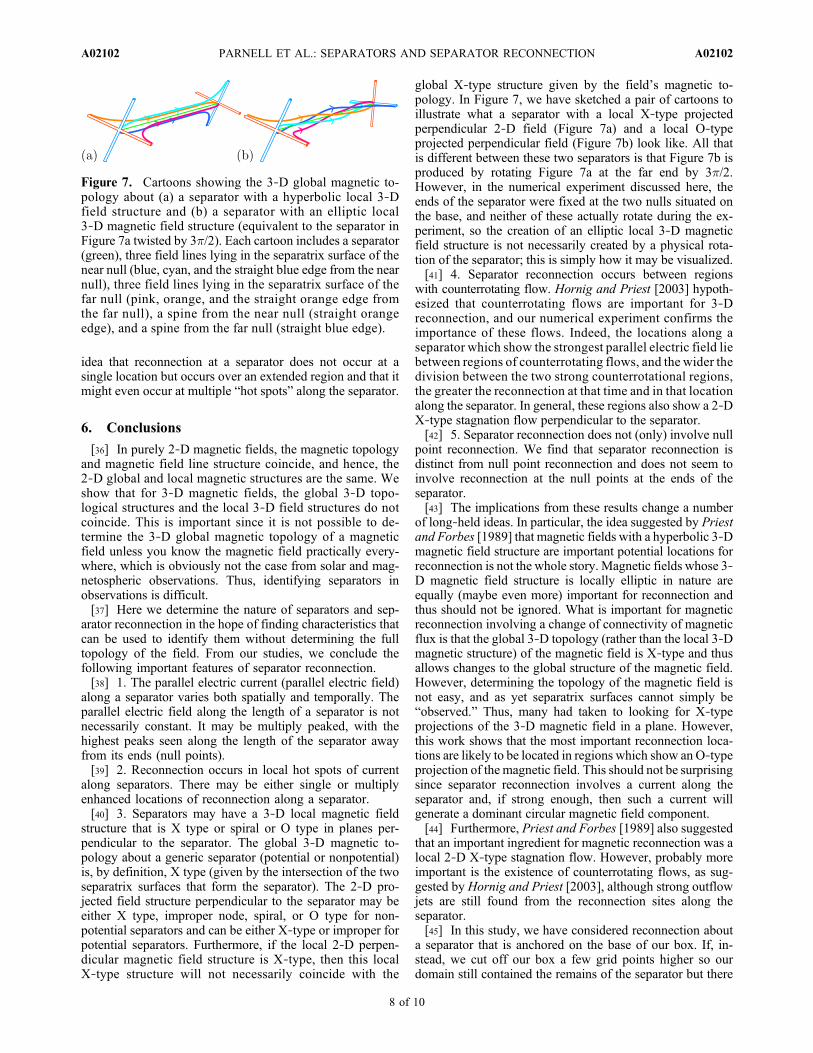
global X‐type structure given by the field’s magnetic to-pology. In Figure 7, we have sketched a pair of cartoons toillustrate what a separator with a local X‐type projectedperpendicular 2‐D field (Figure 7a) and a local O‐typeprojected perpendicular field (Figure 7b) look like. All thatis different between these two separators is that Figure 7b isproduced by rotating Figure 7a at the far end by 3p/2.However, in the numerical experiment discussed here, theends of the separator were fixed at the two nulls situated onthe base, and neither of these actually rotate during the ex-periment, so the creation of an elliptic local 3‐D magneticfield structure is not necessarily created by a physical rota-tion of the separator; this is simply how it may be visualized.[41] 4. Separator reconnection occurs between regions

with counterrotating flow. Hornig and Priest [2003] hypoth-esized that counterrotating flows are important for 3‐Dreconnection, and our numerical experiment confirms theimportance of these flows. Indeed, the locations along aseparator which show the strongest parallel electric field liebetween regions of counterrotating flows, and the wider thedivision between the two strong counterrotational regions,the greater the reconnection at that time and in that locationalong the separator. In general, these regions also show a 2‐DX‐type stagnation flow perpendicular to the separator.[42] 5. Separator reconnection does not (only) involve null

point reconnection. We find that separator reconnection isdistinct from null point reconnection and does not seem toinvolve reconnection at the null points at the ends of theseparator.[43] The implications from these results change a number

of long‐held ideas. In particular, the idea suggested by Priestand Forbes [1989] that magnetic fields with a hyperbolic 3‐Dmagnetic field structure are important potential locations forreconnection is not the whole story. Magnetic fields whose 3‐D magnetic field structure is locally elliptic in nature areequally (maybe even more) important for reconnection andthus should not be ignored. What is important for magneticreconnection involving a change of connectivity of magneticflux is that the global 3‐D topology (rather than the local 3‐Dmagnetic structure) of the magnetic field is X‐type and thusallows changes to the global structure of the magnetic field.However, determining the topology of the magnetic field isnot easy, and as yet separatrix surfaces cannot simply be“observed.” Thus, many had taken to looking for X‐typeprojections of the 3‐D magnetic field in a plane. However,this work shows that the most important reconnection loca-tions are likely to be located in regions which show an O‐typeprojection of the magnetic field. This should not be surprisingsince separator reconnection involves a current along theseparator and, if strong enough, then such a current willgenerate a dominant circular magnetic field component.[44] Furthermore, Priest and Forbes [1989] also suggested

that an important ingredient for magnetic reconnection was alocal 2‐D X‐type stagnation flow. However, probably moreimportant is the existence of counterrotating flows, as sug-gested by Hornig and Priest [2003], although strong outflowjets are still found from the reconnection sites along theseparator.[45] In this study, we have considered reconnection about

a separator that is anchored on the base of our box. If, in-stead, we cut off our box a few grid points higher so ourdomain still contained the remains of the separator but there

Figure 7. Cartoons showing the 3‐D global magnetic to-pology about (a) a separator with a hyperbolic local 3‐Dfield structure and (b) a separator with an elliptic local3‐D magnetic field structure (equivalent to the separator inFigure 7a twisted by 3p/2). Each cartoon includes a separator(green), three field lines lying in the separatrix surface of thenear null (blue, cyan, and the straight blue edge from the nearnull), three field lines lying in the separatrix surface of thefar null (pink, orange, and the straight orange edge fromthe far null), a spine from the near null (straight orangeedge), and a spine from the far null (straight blue edge).

PARNELL ET AL.: SEPARATORS AND SEPARATOR RECONNECTION A02102A02102

8 of 10

were no longer any nulls within our domain, we wouldeffectively have created a quasi‐separator. Since the re-connection found in our experiment occurs along the sep-arator and not at the nulls, we would expect reconnection tooccur in much the same way along our quasi‐separator.Thus, we suspect that reconnection about quasi‐separatorsis likely to be very similar [Titov et al., 2003;Wilmot‐Smithand De Moortel, 2007]. For instance,Wilmot‐Smith and DeMoortel [2007] found that in the middle of their quasi‐separator, where much of their reconnection was occurring,the 2‐D perpendicular magnetic field was elliptic in natureand there was some evidence of counterrotational flows,although in some sense these flows arise simply from thepattern of their driver. However, it is not clear that this is anessential ingredient for 3‐D reconnection. Further studiesneed to be undertaken to investigate the nature of othertypes of reconnecting magnetic structures.[46] Finally, we consider whether the magnetic structure

of separators can be observed. The magnetic field in themagnetosphere is observed using in situ measurements. Forexample, Cluster has four spacecraft and hence can deter-mine all three components of the magnetic field at fourlocations in the magnetosphere simultaneously. Depend-ing on the size of the separator and the extent of the localmagnetic field structure about it, it may be possible toidentify regions that show a 3‐D helical‐like structure, i.e.,with two components of the magnetic field indicating acircular field and the third indicating a single field direc-tion. Evidence of a traditional hyperbolic separator hasbeen found using Cluster data [e.g., Phan et al., 2006];however, as far as the authors know, elliptical separatorfield patterns have not yet been sought. Looking for thesemight be interesting as they are the natural occurrence of ahigh parallel electric field in which reconnection is verylikely to occur, but, of course, they may not be visible ifthe helical structure of the field is very localized.[47] In the solar corona, the magnetic field structure is

inferred from X‐ray or UV images. Since the corona isoptically thin, all the plasma of a given temperature alongthe line of site is observed. Hence, the resulting imagesshow particular magnetic structures, or parts of structures,flattened onto the plane of sky. This means magneticstructures at a different temperature cannot be seen orobservable structures may be obscured from view by otherobservable plasma. Furthermore, structures will appeardifferent depending on the particular plane of sky orien-tation observed (e.g., see the projections of CME magneticfields from the numerical model by Tokman and Bellan[2002]). Therefore, identifying, for example, helical struc-tures will not be easy. Moreover, the sections of the se-parators that have a locally helical field line structure are theregions that have the highest parallel electric fields and arewhere most of the magnetic reconnection is occurring. Insuch regions, prereconnected field lines may not be visible ifthey are too cool, and postreconnected field lines will betransported out of the reconnection site because of the strongoutflow from the reconnection, so they too may not reveal ahelical structure. Finally, the local structure about the sep-arator may be too small to observe with the current imageresolution. In order to properly determine the structures wemight expect to see in the corona in the vicinity of a sepa-rator, we need to forward model the results from a series of

numerical experiments involving separators and calculatecoronal images from various angles. This is outside thescope of the current paper.

[48] Acknowledgments. C.E.P. and A.L.H. would like to thank theLeverhulme Trust: C.E.P. was awarded a Philip Leverhulme Prize in2007 which she is using to support A.L.H. as a research associate. Supportby the European Commission through the Solaire Network (MTRN‐CT‐2006‐035484) is gratefully acknowledged. The authors would like to thankThomas Neukirch and Eric Priest for helpful suggestions in improving thismanuscript.[49] Amitava Bhattacharjee thanks Terry Forbes and another reviewer

for their assistance in evaluating this paper.

ReferencesAulanier, G., E. Pariat, and P. Démoulin (2005), Current sheet formation inquasi‐separatrix layers and hyperbolic flux tubes, Astron. Astrophys.,444, 961–976, doi:10.1051/0004-6361:20053600.

Aulanier, G., E. Pariat, P. Démoulin, and C. R. Devore (2006), Slip‐running reconnection in quasi‐separatrix layers, Sol. Phys., 238(2),347–376, doi:10.1007/s11207-006-0230-2.

Axford, W. I. (1984), Magnetic field reconnection, in Magnetic Reconnec-tion in Space and Laboratory Plasmas, Geophys. Monogr. Ser., vol. 30,edited by E. W. Hones Jr., pp. 1–8, AGU, Washington, D. C.

Biskamp, D. (2000), Magnetic Reconnection in Plasmas, Cambridge Univ.Press, Cambridge, U. K.

Browning, P. K., C. Gerrard, A. W. Hood, R. Kevis, and R. A. M. Van derLinden (2008), Heating the corona by nanoflares: Simulations of energyrelease triggered by a kink instability, Astron. Astrophys., 485, 837–848,doi:10.1051/0004-6361:20079192.

Bungey, T. N., V. S. Titov, and E. R. Priest (1996), Basic topological ele-ments of coronal magnetic fields, Astron. Astrophys., 308, 233–247.

Craig, I. J. D., and R. B. Fabling (1996), Exact solutions for steady state,spine, and fan magnetic reconnection, Astrophys. J., 462, 969–976,doi:10.1086/177210.

Craig, I. J. D., R. B. Fabling, S. M. Henton, and G. J. Rickard (1995), Anexact solution for steady state magnetic reconnection in three dimensions,Astrophys. J., 455, L197, doi:10.1086/309822.

De Moortel, I., and K. Galsgaard (2006a), Numerical modeling of 3Dreconnection due to rotational foot point motions, Astron. Astrophys.,451, 1101–1115, doi:10.1051/0004-6361:20054587.

De Moortel, I., and K. Galsgaard (2006b), Numerical modeling of 3Dreconnection: II. Comparison between rotational and spinning footpoint motions, Astron. Astrophys., 459, 627–639, doi:10.1051/0004-6361:20065716.

Démoulin, P., E. R. Priest, and D. P. Lonie (1996), Three‐dimensionalmagnetic reconnection without null points: 2. Application to twisted fluxtubes, J. Geophys. Res., 101, 7631–7646, doi:10.1029/95JA03558.

Dorelli, J. C., and A. Bhattacharjee (2008), Defining and identifying three‐dimensional magnetic reconnection in resistive magnetohydrodynamicsimulations of Earth’s magnetosphere, Phys. Plasmas, 15, 056504,doi:10.1063/1.2913548.

Galsgaard, K., and Å Nordlund (1997), Heating and activity of the solarcorona: 3. Dynamics of a low beta plasma with three‐dimensional nullpoints, J. Geophys. Res., 102, 231–248, doi:10.1029/96JA02680.

Galsgaard, K., C. E. Parnell, and J. Blaizot (2000a), Elementary heatingevents—Magnetic interactions between two flux sources, Astron.Astrophys., 362, 395–405.

Galsgaard, K., E. R. Priest, and Å Nordlund (2000b), Three‐dimensionalseparator reconnection—How does it occur?, Sol. Phys., 193, 1–16,doi:10.1023/A:1005248811680.

Galsgaard, K., V. S. Titov, and T. Neukirch (2003), Magnetic pinching ofhyperbolic flux tubes. II. Dynamic numerical model, Astrophys. J., 595,506–516, doi:10.1086/377258.

Greene, J. M. (1993), Reconnection of vorticity lines and magnetic lines,Phys. Fluids B, 5, 2355–2362, doi:10.1063/1.860718.

Haynes, A. L. (2007), Magnetic skeletons and 3D magnetic reconnection,Ph.D. thesis, Univ. of St. Andrews, Saint Andrews, U. K.

Haynes, A. L., C. E. Parnell, K. Galsgaard, and E. R. Priest (2007), Mag-netohydrodynamic evolution of magnetic skeletons, Proc. R. Soc. A, 463,1097–1115.

Hesse, M. (1995), Three‐dimensional magnetic reconnection in space‐ andastrophysical plasmas and its consequences for particle acceleration, inCosmic Magnetic Fields, Rev. Mod. Astron., vol. 8, edited by G. Klare,pp. 323–348, Springer, Berlin.

PARNELL ET AL.: SEPARATORS AND SEPARATOR RECONNECTION A02102A02102

9 of 10

Hesse, M., and J. Birn (1993), Parallel electric fields as accelerationmechanisms in three‐dimensional magnetic reconnection, Adv. SpaceRes., 13, 249–252, doi:10.1016/0273-1177(93)90341-8.

Hesse, M., and K. Schindler (1988), A theoretical foundation of generalmagnetic reconnection, J. Geophys. Res., 93, 5559–5567, doi:10.1029/JA093iA06p05559.

Hood, A. W., P. K. Browning, and R. A. M. van der Linden (2009), Coronalheating by magnetic reconnection in loops with zero net current, Astron.Astrophys., 506, 913–925, doi:10.1051/0004-6361/200912285.

Hornig, G., and E. R. Priest (2003), Evolution of magnetic flux in an iso-lated reconnection process, Phys. Plasmas, 10, 2712–2721.

Lau, Y.‐T., and J. Finn (1990), Three‐dimensional kinematic reconnectionin the presence of field nulls and closed field lines, Astrophys. J., 350,672–691.

Linton, M. G., and E. R. Priest (2003), Three‐dimensional reconnection ofuntwisted magnetic flux tubes, Astrophys. J., 595, 1259–1276,doi:10.1086/377439.

Longcope, D. W. (2001), Separator current sheets: Generic features inminimum‐energy magnetic fields subject to flux constraints, Phys.Plasmas, 8, 5277–5290, doi:10.1063/1.1418431.

Longcope, D. W., and S. C. Cowley (1996), Current sheet formation alongthree‐dimensional magnetic separators, Phys. Plasmas, 3, 2885–2897,doi:10.1063/1.871627.

Parnell, C. E., A. L. Haynes, and K. Galsgaard (2008), Recursive reconnec-tion and magnetic skeletons, Astrophys. J., 675, 1656–1665, doi:10.1086/527532.

Phan, T. D., et al. (2006), A magnetic reconnection X‐line extending morethan 390 Earth radii in the solar wind, Nature, 439, 175–178.

Pontin, D. I., and I. J. D. Craig (2005), Current singularities at finitely com-pressible three‐dimensional magnetic null points, Phys. Plasmas, 12,072112, doi:10.1063/1.1987379.

Pontin, D. I, and I. J. D. Craig (2006), Dynamic three‐dimensional recon-nection in a separator geometry with two null points, Astrophys. J., 642,568–578.

Pontin, D. I., and K. Galsgaard (2007), Current amplification and magneticreconnection at a three‐dimensional null point: Physical characteristics,J. Geophys. Res., 112, A03103, doi:10.1029/2006JA011848.

Pontin, D. I., K. Galsgaard, G. Hornig, and E. R. Priest (2005a), A fullymagnetohydrodynamic simulation of three‐dimensional non‐null recon-nection, Phys. Plasmas, 12, 052307, doi:10.1063/1.1891005.

Pontin, D. I., G. Hornig, and E. R. Priest (2005b), Kinematic reconnectionat a magnetic null point: Fan‐aligned current, Geophys. Astrophys. FluidDyn., 99, 77–93.

Pontin, D. I., A. Bhattacharjee, and K. Galsgaard (2007a), Current sheetformation and nonideal behavior at three‐dimensional magnetic nullpoints, Phys. Plasmas, 14, 052106, doi:10.1063/1.2722300.

Pontin, D. I., A. Bhattacharjee, and K. Galsgaard (2007b), Current sheets atthree‐dimensional magnetic nulls: Effect of compressibility, Phys. Plasmas,14, 052109, doi:10.1063/1.2734949.

Priest, E. R., and P. Démoulin (1995), Three‐dimensional magnetic recon-nection without null points: 1. Basic theory of magnetic flipping, J.Geophys. Res., 100, 23,443–23,464, doi:10.1029/95JA02740.

Priest, E. R., and T. G. Forbes (1989), Steady magnetic reconnection inthree dimensions, Sol. Phys., 119, 211–214, doi:10.1007/BF00146222.

Priest, E. R., and T. G. Forbes (2000),Magnetic Reconnection: MHD Theoryand Applications, Cambridge Univ. Press, Cambridge, U. K.

Priest, E. R., and V. S. Titov (1996), Magnetic reconnection at three‐dimensional null points, Philos. Trans. R. Soc. A, 355, 2951–2992.

Schindler, K., M. Hesse, and J. Birn (1988), General magnetic reconnec-tion, parallel electric fields, and helicity, J. Geophys. Res., 93, 5547–5557, doi:10.1029/JA093iA06p05547.

Sonnerup, B. U. Ö. (1979), Magnetic field reconnection, in Space PlasmaPhysics: The Study of Solar‐System Plasmas, vol. 2, 879–972, Natl.Acad. Press, Washington, D. C.

Titov, V. S., K. Galsgaard, and T. Neukirch (2003), Magnetic pinching ofhyperbolic flux tubes. I. Basic estimations, Astrophys. J., 582, 1172–1189, doi:10.1086/344799.

Titov, V. S., T. G. Forbes, E. R. Priest, Z. Mikić, and J. A. Linker (2009),Slip‐squashing factors as a measure of three‐dimensional magneticreconnection, Astrophys. J., 693, 1029–1044, doi:10.1088/0004-637X/693/1/1029.

Tokman, M., and P. M. Bellan (2002), Three‐dimensional model of thestructure and evolution of coronal mass ejections, Astrophys. J., 567,1202–1210, doi:10.1086/338699.

Vasyliunas, V. M. (1975), Theoretical models of magnetic field line merg-ing, Rev. Geophys., 13, 303–336.

Wilmot‐Smith, A. L., and I. De Moortel (2007), Magnetic reconnection influx tubes undergoing spinning foot point motions, Astron. Astrophys.,473, 615–623, doi:10.1051/0004-6361:20077455.

K. Galsgaard, Niels Bohr Institute, Julie Maries vej 30, DK‐2100Copenhagen, Denmark. (kg@astro.ku.dk)A. L. Haynes and C. E. Parnell, School of Mathematics and Statistics,

University of St. Andrews, Saint Andrews KY16 9SS, UK. (andrew@mcs.st‐andrews.ac.uk; clare@mcs.st‐andrews.ac.uk)

PARNELL ET AL.: SEPARATORS AND SEPARATOR RECONNECTION A02102A02102

10 of 10