Embed Size (px)
Citation preview
10 Strongly Correlated Superconductivity
Andre-Marie S. TremblayDepartement de physiqueRegroupement quebecois sur les materiaux de pointeCanadian Institute for Advanced ResearchSherbrooke, Quebec J1K 2R1, Canada
Contents1 Introduction 2
2 The Hubbard model 3
3 Weakly and strongly correlated antiferromagnets 43.1 Antiferromagnets: A qualitative discussion . . . . . . . . . . . . . . . . . . . 53.2 Contrasting methods for weak and strong coupling antiferromagnets
and their normal state . . . . . . . . . . . . . . . . . . . . . . . . . . . . . . . 7
4 Weakly and strongly correlated superconductivity 94.1 Superconductors: A qualitative discussion . . . . . . . . . . . . . . . . . . . . 94.2 Contrasting methods for weakly and strongly correlated superconductors . . . . 11
5 High-temperature superconductors and organics:the view from dynamical mean-field theory 155.1 Quantum cluster approaches . . . . . . . . . . . . . . . . . . . . . . . . . . . 165.2 Normal state and pseudogap . . . . . . . . . . . . . . . . . . . . . . . . . . . 205.3 Superconducting state . . . . . . . . . . . . . . . . . . . . . . . . . . . . . . . 24
6 Conclusion 30
E. Pavarini, E. Koch, and U. SchollwockEmergent Phenomena in Correlated MatterModeling and Simulation Vol. 3Forschungszentrum Julich, 2013, ISBN 978-3-89336-884-6http://www.cond-mat.de/events/correl13

10.2 Andre-Marie S. Tremblay
1 Introduction
Band theory and the BCS-Eliashberg theory of superconductivity are arguably the most suc-cessful theories of condensed matter physics by the breadth and subtlety of the phenomena theyexplain. Experimental discoveries, however, clearly signal their failure in certain cases. Around1940, it was discovered that some materials with an odd number of electrons per unit cell, forexample NiO, were insulators instead of metals, a failure of band theory [1]. Peierls and Mottquickly realized that strong effective repulsion between electrons could explain this (Mott) in-sulating behaviour [2]. In 1979 and 1980, heavy fermion [3] and organic [4] superconductorswere discovered, an apparent failure of BCS theory because the proximity of the superconduct-ing phases to antiferromagnetism suggested the presence of strong electron-electron repulsion,contrary to the expected phonon-mediated attraction that gives rise to superconductivity in BCS.Superconductivity in the cuprates [5], in layered organic superconductors [6,7], and in the pnic-tides [8] eventually followed the pattern: superconductivity appeared at the frontier of antiferro-magnetism and, in the case of the layered organics, at the frontier of the Mott transition [9, 10],providing even more examples of superconductors falling outside the BCS paradigm [11, 12].The materials that fall outside the range of applicability of band and of BCS theory are oftencalled strongly correlated or quantum materials. They often exhibit spectacular properties, suchas colossal magnetoresistance, giant thermopower, high-temperature superconductivity etc.
The failures of band theory and of the BCS-Eliashberg theory of superconductivity are in factintimately related. In these lecture notes, we will be particularly concerned with the failure ofBCS theory, and with the understanding of materials belonging to this category that we callstrongly correlated superconductors. These superconductors have a normal state that is not asimple Fermi liquid and they exhibit surprising superconducting properties. For example, inthe case of layered organic superconductors, they become better superconductors as the Motttransition to the insulating phase is approached [13].
These lecture notes are not a review article. The field is still evolving rapidly, even after morethan 30 years of research. My aim is to provide for the student at this school an overview ofthe context and of some important concepts and results. I try to provide entries to the literatureeven for topics that are not discussed in detail here. Nevertheless, the reference list is far fromexhaustive. An exhaustive list of all the references for just a few sub-topics would take morethan the total number of pages I am allowed.
I will begin by introducing the one-band Hubbard model as the simplest model that containsthe physics of interest, in particular the Mott transition. That model is 50 years old this year[14–16], yet it is far from fully understood. Section 3 will use antiferromagnetism as an exampleto introduce notions of weak and strong correlations and to contrast the theoretical methods thatare used in both limits. Section 4 will do the same for superconductivity. Finally, Section 5will explain some of the most recent results obtained with cluster generalizations of dynamicalmean-field theory, approaches that allow one to explore the weak and strong correlation limitsand the transition between both.

Strongly Correlated Superconductivity 10.3
2 The Hubbard model
The one-band Hubbard model is given by
H = −
i,j,σ
tijc†iσcjσ + U
i
ni↑ni↓ (1)
where i and j label Wannier states on a lattice, c†iσ and ciσ are creation and annihilation operatorsfor electrons of spin σ, niσ = c
†iσciσ is the number of spin σ electrons on site i, tij = t
∗ji are
the hopping amplitudes, which can be taken as real in our case, and U is the on-site Coulombrepulsion. In general, we write t, t
, t
respectively for the first-, second-, and third-nearestneighbour hopping amplitudes.
This model is a drastic simplification of the complete many-body Hamiltonian, but we wantto use it to understand the physics from the simplest point of view, without a large number ofparameters. The first term of the Hubbard model Eq. (1) is diagonal in a momentum-spacesingle-particle basis, the Bloch waves. There, the wave nature of the electron is manifest. If theinteraction U is small compared to the bandwidth, perturbation theory and Fermi liquid theoryhold [17, 18]. This is called the weak-coupling limit.
The interaction term in the Hubbard Hamiltonian, proportional to U , is diagonal in positionspace, i.e., in the Wannier orbital basis, exhibiting the particle nature of the electron. The mo-tivation for that term is that once the interactions between electrons are screened, the dominantpart of the interaction is on-site. Strong-coupling perturbation theory can be used if the band-width is small compared with the interaction [19–23].
Clearly, the intermediate-coupling limit will be most difficult, the electron exhibiting both waveand particle properties at once. The ground state will be entangled, i.e. very far from a productstate of either Bloch (plane waves) of Wannier (localized) orbitals. We refer to materials in thestrong or intermediate-coupling limits as strongly correlated.
When the interaction is the largest term and we are at half-filling, the solution of this Hamil-tonian is a Mott insulating state. The ground state will be antiferromagnetic if there is nottoo much frustration. That can be seen as follows. If hopping vanishes, the ground state is2N -fold degenerate if there are N sites. Turning-on nearest-neighbour hopping, second or-
der degenerate perturbation theory in t leads to an antiferromagnetic interaction JSi · Sj withJ = 4t
2/U [24, 25]. This is the Heisenberg model. Since J is positive, this term will be small-
est for anti-parallel spins. The energy is generally lowered in second-order perturbation theory.Parallel spins cannot lower their energy through this mechanism because the Pauli principle for-bids the virtual, doubly occupied state. P.W. Anderson first proposed that the strong-couplingversion of the Hubbard model could explain high-temperature superconductors [26].
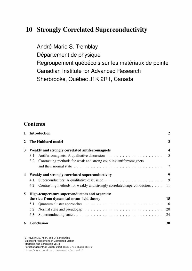
A caricature of the difference between an ordinary band insulator and a Mott insulator is shownin Figure 1. Refer to the explanations in the caption.
10.4 Andre-Marie S. Tremblay
Fig. 1: Figure from Ref. [27]. In a band insulator, as illustrated on the top-left figure, thevalence band is filled. For N sites on the lattice, there are 2N states in the valence band,the factor of 2 accounting for spins, and 2N states in the conduction band. PES on the fig-ures refers to “Photoemission Spectrum” and IPES to “Inverse Photoemission Spectrum”. Thesmall horizontal lines represent energy levels and the dots stand for electrons. In a Mott in-sulator, illustrated on the top-right figure, there are N states in the lower energy band (LowerHubbard band) and N in the higher energy band (Upper Hubbard band), for a total of 2N aswe expect in a single band. The two bands are separated by an energy U because if we add anelectron to the already occupied states, it costs an energy U . Perhaps the most striking differ-ence between a band and a Mott insulator manifests itself when the Fermi energy EF is movedto dope the system with one hole. For the semiconductor, the Fermi energy moves, but the banddoes not rearrange itself. There is one unoccupied state right above the Fermi energy. Thisis seen on the bottom-left figure. On the bottom-right figure, we see that the situation is verydifferent for a doped Mott insulator. With one electron missing, there are two states just abovethe Fermi energy, not one state only. Indeed one can add an electron with a spin up or down onthe now unoccupied site. And only N ! 1 states are left that will cost an additional energy U ifwe add an electron. Similarly, N ! 1 states survive below the Fermi energy.
3 Weakly and strongly correlated antiferromagnets
A phase of matter is characterized by very general “emergent” properties, i.e., properties thatare qualitatively different from those of constituent atoms [28–30]. For example, metals areshiny and they transport DC current. These are not properties of individual copper or goldatoms. It takes a finite amount of energy to excite these atoms from their ground state, so theycannot transport DC current. Also, their optical spectrum is made of discrete lines whereasmetals reflect a continuous spectrum of light at low energy. In other words, the Fermi surfaceis an emergent property. Even in the presence of interactions, there is a jump in momentum
Strongly Correlated Superconductivity 10.5
occupation number that defines the Fermi surface. This is the Landau Fermi liquid [17, 18].Emergent properties appear at low energy, i.e., for excitation energies not far from the groundstate. The same emergent properties arise from many different models. In the renormalizationgroup language, phases are trivial fixed points, and many Hamiltonians flow to the same fixedpoint.In this section, we use the antiferromagnetic phase to illustrate further what is meant by anemergent property and what properties of a phase depend qualitatively on whether we are dom-inated by band effects or by strong correlations. Theoretical methods appropriate for each limitare described in the last subsection.
3.1 Antiferromagnets: A qualitative discussion
Consider the nearest-neighbour Hubbard model at half-filling on the cubic lattice in three di-mensions. At T = 0, there is a single phase, an antiferromagnet, whatever the value of theinteraction U . One can increase U continuously without encountering a phase transition. Thereis an order parameter in the sense of Landau, in this case the staggered magnetization. This orderparameter reflects the presence of a broken symmetry: time reversal, spin rotational symmetryand translation by a lattice spacing are broken, while time reversal accompanied by translationby a lattice spacing is preserved.A single-particle gap and spin waves as Goldstone modes are emergent consequences of thisbroken symmetry. Despite the fact that we are in a single phase, there are qualitative differencesbetween weak and strong coupling as soon as we probe higher energies. For example, at strong-coupling spin waves, at an energy scale of J , persist throughout the Brillouin zone, whereas atweak coupling they enter the particle-hole continuum and become Landau damped before wereach the zone boundary. The ordered moment is saturated to its maximum value when U islarge enough but it can become arbitrarily small as U decreases.The differences between weak and strong coupling are also striking at finite temperature. This isillustrated in a schematic fashion in Fig. 2a. The Neel temperature TN , increases as we increaseU because the instability of the normal state fundamentally comes from nesting. In other words,thinking again of perturbation theory, the flat parts of the Fermi surface are connected by theantiferromagnetic wave vector Q = (π, π) which implies a vanishing energy denominator atthat wave vector and thus large spin susceptibility χ with a phase transition occuring when Uχ
is large enough. At strong coupling, TN decreases with increasing U because the spin stiffness isproportional to J = 4t
2/U . Since we can in principle vary the ratio t/U by changing pressure,
it is clear that the pressure derivative of the Neel temperature has opposite sign at weak andstrong coupling. The normal state is also very different. If we approach the transition from theleft, as indicated by the arrow marked ”Slater”, we are in a metallic phase. We also say that theantiferromagnet that is born out of this metallic phase is an itinerant antiferromagnet. On thecontrary, approaching the transition from the right, we come from an insulating (gapped) phasedescribed by the Heisenberg model. Increasing U at fixed T above the maximum TN , we haveto cross over from a metal, that has a Fermi surface, to an insulator, that has local moments, a

10.6 Andre-Marie S. Tremblay
J = 4t2 /U
T
U
AFM
SlaterHeisenberg
Mott
U
T
M I
(a)
(b)
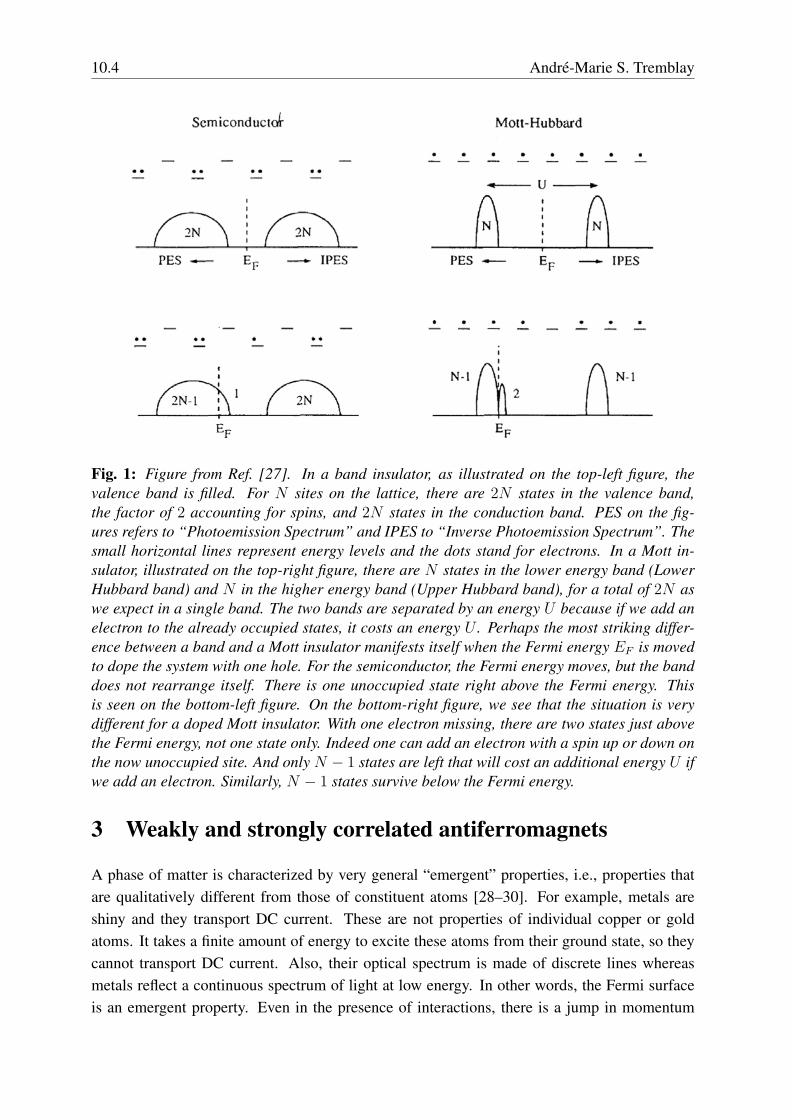
Fig. 2: Schematic phase diagram of the half-filled 3d Hubbard model in the temperature T
vs. interaction U plane for perfect nesting. (a) The solid red line is the Neel temperature TN
below which the system is antiferromagnetic. Coming from the left, it is a metallic state thatbecomes unstable to antiferromagnetism by the Slater mechanism. Coming from the right, itis a gapped insulator with local moments described by the Heisenberg model that becomesunstable to antiferromagnetism. The dashed green line above the maximum TN indicates acrossover from a metallic state with a Fermi surface to a gapped state with local moments.That crossover can be understood in (b) where antiferromagnetism is prevented from occurring.There dynamical mean-field theory predicts a first-order phase transition between a metal anda Mott insulator, with a coexistence region indicated in blue.
gap, and no Fermi surface. This highly non-trivial physics is indicated by a dashed green linein Fig. 2a and marked “Mott” [31].Fig. 2b illustrates another way to understand the dashed green line. Imagine that antiferro-magnetism does not occur before we reach zero temperature. This can be achieved in two di-mensions where the Mermin-Wagner-Hohenberg [32,33] theorem prevents a broken continuoussymmetry at finite temperature. More generally antiferromagnetism can be prevented by frus-tration [34]. Frustration can come either from longer-range hopping that leads to longer-rangeantiferromagnetic interactions or from the geometry of the lattice (e.g. the triangular lattice). Ineither case, it becomes impossible to minimize the energy of all the individual antiferromagneticbonds without entering a contradiction. In Dynamical Mean-Field Theory [35–37], which we
Strongly Correlated Superconductivity 10.7
will discuss later in more detail, antiferromagnetism can simply be prevented from occurring inthe theory. In any case, what happens in the absence of antiferromagnetism is a first-order tran-sition at T = 0 between a metal and an insulator. This is the Mott phase transition that ends at acritical temperature. This transition is seen, for example, in layered organic superconductors ofthe κ-BEDT family that we will briefly discuss later [6, 7]. The dashed green line at finite tem-perature is the crossover due to this transition. In the case where the antiferromagnetic phase isartificially prevented from occurring, the metallic and insulating phases at low temperature aremetastable in the same way that the normal metal is a metastable state below the superconduct-ing transition temperature. Just as it is useful to think of a Fermi liquid at zero temperature evenwhen it is not the true ground state, it is useful to think of the zero-temperature Mott insulatoreven when it is a metastable state.
3.2 Contrasting methods for weak and strong coupling antiferromagnetsand their normal state
In this subsection, I list some of the approaches that can be used to study the various limitingcases as well as their domain of applicability wherever possible. Note that the antiferromagneticstate can occur away from half-filling as well, so we also discuss states that would be bestcharacterized as Fermi liquids.
3.2.1 Ordered state
The ordered state at weak coupling can be described for example by mean-field theory applieddirectly to the Hubbard model [38]. Considering spin waves as collective modes, one canproceed by analogy with phonons and compute the corresponding self-energy resulting from theexchange of spin waves. The staggered moment can then be obtained from the resulting Greenfunction. It seems that this scheme interpolates smoothly and correctly from weak to strongcoupling. More specifically, at very strong coupling in the T = 0 limit, the order parameter isrenormalized down from its bare mean-field value by an amount very close to that predicted ina localized picture with a spin wave analysis of the Heisenberg model: In two dimensions onthe square lattice, only two thirds of the full moment survives the zero-point fluctuations [39].This is observed experimentally in the parent high-temperature superconductor La2CuO4 [40].At strong coupling when the normal state is gapped, one can perform degenerate perturbationtheory, or systematically apply canonical transformations to obtain an effective model [41, 42]that reduces to the Heisenberg model at very strong coupling. When the interaction is not strongenough, higher order corrections in t/U enter in the form of longer-range exchange interactionsand so-called ring-exchanges [41–45]. Various methods such as 1/S expansions [46], 1/Nexpansions [47] or non-linear sigma models [48] are available.Numerically, stochastic series expansions [49], high-temperature series expansions [50], quan-tum Monte Carlo (QMC) [51], world-line or worm algorithms [52, 53], and variational meth-ods [54] are popular and accurate. Variational methods can be biased since one must guess a

10.8 Andre-Marie S. Tremblay
wave function. Nevertheless, variational methods [55] and QMC have shown that in two di-mensions, on the square lattice, the antiferromagnetic ground state is most likely [56]. Statesdescribed by singlet formation at various length scales, so-called resonating valence bond spinliquids, are less stable. For introductions to various numerical methods, see the web archives ofthe summer schools [57] and [58].
3.2.2 The normal state
In strong coupling, the normal state is an insulator described mostly by the non-linear sigmamodel [59,60]. In the weak-coupling limit, the normal state is a metal described by Fermi liquidtheory. To describe a normal state that can contain strong antiferromagnetic fluctuations [61],one needs to consider a version of Fermi liquid theory that holds on a lattice. Spin propagatesin a diffusive manner. These collective modes are known as paramagnons. The instability of thenormal state to antiferromagnetism can be studied by the random phase approximation (RPA),by self-consistent-renormalized theory (SCR) [62], by the fluctuation exchange approximation(FLEX) [63,64], by the functional renormalization group (FRG) [65–67], by field-theory meth-ods [68, 69], and by the two-particle self-consistent approach (TPSC) [70–72], to give someexamples. Numerically, quantum Monte Carlo (QMC) is accurate and can serve as benchmark,but in many cases it cannot go to very low temperature because of the sign problem. That prob-lem does not occur in the half-filled nearest-neighbor one-band Hubbard model, which can bestudied at very low temperature with QMC [73].The limitations of most of the above approaches have been discussed in the Appendices ofRef. [70]. Concerning TPSC, in short, it is non-perturbative and the most accurate of the analyt-ical approaches at weak to intermadiate coupling, as judged from benchmark QMC [70,72,74].TPSC also satisfies the Pauli principle in the sense that the square of the occupation number forone spin species on a lattice site is equal to the occupation number itself, in other words 12 = 1
and 02= 0. RPA is an example of a well known theory that violates this constraint (see, e.g.,
Appendix A3 of Ref. [70]). Also, TPSC satisfies conservation laws and a number of sum rules,including those which relate the spin susceptibility to the local moment and the charge suscep-tibility to the local charge. Most importantly, TPSC satisfies the Mermin-Wagner-Hohenbergtheorem in two dimensions, contrary to RPA. Another effect included in TPSC is the renor-malization of U coming from cross channels (Kanamori, Bruckner screening) [15, 75]. On amore technical level, TPSC does not assume a Migdal theorem in the calculation of the self-energy and the trace of the matrix product of the self-energy with the Green function satisfiesthe constraint that it is equal to twice the potential energy.The most important prediction that came out of TPSC for the normal state on the two-dimensionalsquare lattice, is that precursors of the antiferromagnetic ground state will occur when theantiferromagnetic correlation length becomes larger than the thermal de Broglie wave lengthvF/kBT [76–78]. The latter is defined by the inverse of the wave vector spread that is causedby thermal excitations ∆ε ∼ kBT . This result was verified experimentally [79] and it explainsthe pseudogap in electron-doped high-temperature superconductors [72, 80, 81].

Strongly Correlated Superconductivity 10.9
4 Weakly and strongly correlated superconductivity
As discussed in the previous section, antiferromagnets have different properties depending onwhether U is above or below the Mott transition, and appropriate theoretical methods mustbe chosen depending on the case. In this section, we discuss the analogous phenomenon forsuperconductivity. A priori, the superconducting state of a doped Mott insulator or a dopeditinerant antiferromagnet are qualitatively different, even though some emergent properties aresimilar.
4.1 Superconductors: A qualitative discussion
As for antiferromagnets, the superconducting phase has emergent properties. For an s-wavesuperconductor, global charge conservation, or U(1) symmetry, is broken. For a d-wave su-perconductor, in addition to breaking U(1) symmetry, the order parameter does not transformtrivially under rotation by π/2. It breaks the C4v symmetry of the square lattice. In both caseswe have singlet superconductivity, i.e., spin-rotational symmetry is preserved. In both cases,long-range forces push the Goldstone modes to the plasma frequency by the Anderson-Higgsmechanism [82]. The presence of symmetry-dictated nodes in the d-wave case is an emergentproperty with important experimental consequences: for example, the specific heat will vanishlinearly with temperature and similarly for the thermal conductivity κ. The ratio κ/T reachesa universal constant in the T = 0 limit, i.e., that ratio is independent of disorder [83, 84]. Theexistence of a single-particle gap with nodes determined by symmetry is also an emergent prop-erty, but its detailed angular dependence and its size relative to other quantities, such as thetransition temperature Tc, is dependent on details.A possible source of confusion in terminology is that in the context of phonon mediated s-wavesuperconductivity, there is the notion of strong-coupling superconductivity. The word strong-coupling has a slightly different meaning from the one discussed up to now. The context shouldmake it clear what we are discussing. Eliashberg theory describes phonon-mediated strong-coupling superconductivity [85–89]. In that case, quasiparticles survive the strong electron-phonon interaction, contrary to the case where strong electron-electron interactions destroy thequasiparticles in favour of local moments in the Mott insulator.There are important quantitative differences between BCS and Eliashberg superconductors. Inthe latter case, the self-energy becomes frequency dependent so one can measure the effect ofphonons on a frequency dependent gap function that influences in turn the tunnelling spectra.Predictions for the critical field Hc(T ) or for the ratio of the gap to Tc for example differ. TheEliashberg approach is the most accurate.Let us return to our case, namely superconductors that arise from a doped Mott insulator(strongly correlated) and superconductors that arise from doping an itinerant antiferromag-net (weakly correlated). Again there are differences between both types of superconductorswhen we study more than just asymptotically small frequencies. For example, as we will seein Section 5, in strongly correlated superconductors, the gap is no-longer particle-hole sym-

10.10 Andre-Marie S. Tremblay
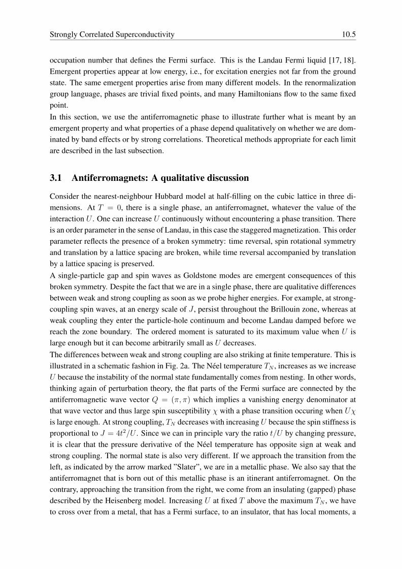
Fig. 3: Absorption spectrum for a sharp atomic level whose energy is about 0.5 keV below theFermi level. At half-filling, or zero doping x = 0, it takes about 530 eV to excite an electronfrom the deep level to the upper Hubbard band. As one dopes, the upper Hubbard band stillabsorbs, but new states appear just above the Fermi level, allowing the X-ray to be absorbedat an energy about 2 eV below the upper Hubbard band. These states are illustrated on thebottom right panel of Fig. 1. The important point is that the spectral weight in the states justabove the Fermi energy grows about twice as fast as the spectral weight in the upper Hubbardband decreases, in agreement with the cartoon picture of a doped Mott insulator. Figure fromRef. [102]
metric, and the transition temperature sometimes does not scale like the order parameter. Astrongly-coupled superconductor is also more resilient to nearest-neighbor repulsion than aweakly-coupled one [90].
We should add a third category of strongly-correlated superconductors, namely superconductorsthat arise, in the context of the Hubbard model, at half-filling under a change of pressure. This isthe case of the layered organics. There again superconductivity is very special since, contrary tonaive expectations, it becomes stronger as we approach the Mott metal-insulator transition [13].
Just as for antiferromagnets, the normal state of weakly-correlated and of strongly-correlated su-perconductors is very different. Within the one-band Hubbard model as usual, the normal stateof weakly-correlated superconductors is a Fermi liquid with antiferromagnetic fluctuations. Inthe case of strongly correlated superconductors, the normal state exhibits many strange proper-ties, the most famous of which is probably the linear temperature dependence of resistivity thatpersists well above the Mott-Ioffe-Regel (MIR) limit [91–93]. This limit is defined as follows:Consider a simple Drude formula for the conductivity, σ = ne
2τ/m, where n is the density,
e is the electron charge, m the mass, and τ the collision time. Using the Fermi velocity vF ,one can convert the scattering time τ to a mean-free path . The MIR minimal conductivityis determined by stating that the mean-free path cannot be smaller than the Fermi wavelength.This means that, as a function of temperature, resistivity should saturate to that limit. This is

Strongly Correlated Superconductivity 10.11
seen in detailed many-body calculations with TPSC [94] (These calculations do not include thepossibility of the Mott transition). For a set of two-dimensional planes separated by a distanced, the MIR limit is set by d/e2. That limit can be exceeded in doped Mott insulators [93, 95].The strange-metal properties, including the linear temperature dependence of the resistivity, areoften considered as emergent properties of a new phase. Since new phases of matter are difficultto predict, one approach has been to find mean-field solutions of gauge-field theories. Thesegauge theories can be derived from Hubbard-Stratonovich transformations or from assumptionsas to the nature of the emergent degrees of freedom [96].As in the case of the antiferromagnet, the state above the optimal transition temperature instrongly correlated superconductors is a state where crossovers occur. There is much evi-dence that hole-doped high-temperature superconductors are doped Mott insulators. The high-temperature thermopower [97,98] and Hall coefficient [99] are examples of properties that are asexpected from Mott insulators. We can verify the doped Mott insulator nature of the hole-dopedcuprates from the experimental results for soft X-ray absorption spectroscopy as illustrated inFig. 3. This figure should be compared with the cartoon in Fig. 1. More recent experimentalresults on this topic [100] and comparison with the Hubbard model [101] are available in theliterature.
4.2 Contrasting methods for weakly and strongly correlatedsuperconductors
In most phase transitions, a simple analysis at weak coupling indicates that the normal stateis unstable towards a new phase. For example, one can compute an appropriate susceptibil-ity in the normal state and observe that it can sometimes diverge at sufficiently low tempera-ture, indicating an instability. For an antiferromagnet, we would compute the staggered spin-susceptibility. Alternatively, one could perform a mean-field factorization and verify that thereis a self-consistent broken symmetry solution at low temperature. Neither of these two pro-cedures however leads to a superconducting instability when we start from a purely repulsiveHubbard model. In this section, we will discuss how to overcome this.Surprisingly, a mean-field factorization of the Hubbard model at strong coupling does lead toa superconducting d-wave ground state [103–105]. There are reasons, however, to doubt theapproximations involved in a simple mean-field theory at strong coupling.
4.2.1 The normal state and its superconducting instability
In the weakly correlated case, the normal state must contain slow modes that replace thephonons to obtain a superconducting instability. It is as if the superconducting instability cameat a second level of refinement of the theory. This all started with Kohn and Luttinger [106,107]:They noted that the interaction between two electrons is screened by the other electrons. Com-puting this screening to leading order, they found that in sufficiently high angular-momentumstates and at sufficiently low temperature (usually very low) there is always a superconducting

10.12 Andre-Marie S. Tremblay
instability in a Fermi liquid (see, e.g., Ref. [108] for a review). It is possible to do calculationsin this spirit that are exact for infinitesimally small repulsive interactions [109].Around 1986, before the discovery of high-temperature superconductivity, it was realized thatif instead of a Fermi liquid in a continuum, one considers electrons on a lattice interactingwith short-range repulsion, then the superconducting instability may occur more readily. Morespecifically, it was found that exchange of antiferromagnetic paramagnons between electronscan lead to a d-wave superconducting instability [110, 111]. This is somewhat analogous towhat happens for ferromagnetic fluctuations in superfluid 3He (for a recent exhaustive reviewof unconventional superconductivity, see Ref. [112]). These types of theories [113], like TPSCbelow, have some features that are qualitatively different from the BCS prediction [114, 115].For example, the pairing symmetry depends more on the shape of the Fermi surface than on thesingle-particle density of states. Indeed, the shape of the Fermi surface determines the wavevector of the largest spin fluctuations, which in turn favor a given symmetry of the d-waveorder parameter, for example dx2−y2 vs. dxy [116], depending on whether the antiferromagneticfluctuations are in the (π, π) or (π, 0) direction, respectively. It is also believed that conditionsfor maximal Tc are realized close to the quantum critical point of an apparently competingphase, such as an antiferromagnetic phase [117, 118], or a charge ordered phase [119].In the case of quasi-one-dimensional conductors, a more satisfying way of obtaining d-wave su-perconductivity in the presence of repulsion consists of using the renormalization group [120,121]. In this approach, one finds a succession of effective low-energy theories by eliminat-ing perturbatively states that are far away from the Fermi surface. As more and more degreesof freedom are eliminated, i.e., as the cutoff decreases, the effective interactions for the low-energy theory can grow or decrease, or even change sign. In this approach then, all fluctuationchannels are considered simultaneously, interfering with and influencing each other. The ef-fective interaction in the particle-particle d-wave channel can become attractive, signalling asuperconducting instability.Whereas this approach is well justified in the one-dimensional and quasi one-dimensional casesfrom the logarithmic behavior of perturbation theory, in two dimensions more work is needed.Nevertheless, allowing the renormalized interactions to depend on all possible momenta, onecan devise the so-called functional renormalization group. One can follow either the Wilsonprocedure [67], as was done orginally for fermions by Bourbonnais [122, 123], or a functionalapproach [65,66] closer in spirit to quantum field-theory approaches. d-wave superconductivityhas been found in these approaches [124–126].As we have already mentioned, in two dimensions, even at weak to intermediate coupling, thenormal state out of which d-wave superconductivity emerges is not necessarily a simple Fermiliquid. It can have a pseudogap induced by antiferromagnetic fluctuations. Because TPSCis the only approach that can produce a pseudogap in two dimensions over a broad range oftemperature, we mention some of the results of this approach [116,127]. The approach is similarin spirit to the paramagnon theories above [110, 111, 113], but it is more appropriate because,as mentioned before, it satisfies the Mermin-Wagner theorem, is non-perturbative, and satisfiesa number of sum rules. The irreducible vertex in the particle-particle channel is obtained from
Strongly Correlated Superconductivity 10.13
functional derivatives. Here are some of the main results:
1. The pseudogap appears when the antiferromagnetic correlation length exceeds the ther-mal de Broglie wave length. This is why, even without competing order, Tc decreasesas one approaches half-filling despite the fact that the AFM correlation length increases.This can be seen in Fig. 3 of Ref [127]. States are removed from the Fermi level and hencecannot lead to pairing. The dome is less pronounced when second-neighbor hopping t
is finite because the fraction of the Fermi surface where states are removed (hot spots) issmaller.
2. The superconducting Tc depends rather strongly on t. At fixed filling, there is an optimal
frustration, namely a value of t where Tc is maximum as illustrated in Fig. 5 of Ref. [116].
3. Fig. 6 of Ref. [116] shows that Tc can occur below the pseudogap temperature or above.(The caption should read U = 6 instead of U = 4). For the cases considered, that includeoptimal frustration, the AFM correlation length at the maximum Tc is about 9 latticespacings, as in Ref. [128]. Elsewhere, it takes larger values at Tc.
4. A correlation between resistivity and Tc in the pnictides, the electron-doped cuprates, andthe quasi one-dimensional organics was well established experimentally in Ref. [129].Theoretically it is well understood for the quasi one-dimensional organics [121]. (It seemsto be satisfied in TPSC, as illustrated by Fig. 5 of Ref. [81], but the analytical continuationhas some uncertainties.)
5. There is strong evidence that the electron-doped cuprates provide an example where anti-ferromagnetically mediated superconductivity can be verified. Figs. 3 and 4 of the paperby the Greven group [79] show that at optimal Tc the AFM correlation length is of theorder of 10 lattice spacings. The photoemission spectrum and the AFM correlation lengthobtained from the Hubbard model [80] with t
= −0.175 t, t
= 0.05 t and U = 6.25 t
agree with experiment. In particular, in TPSC one obtains the dynamical exponent z = 1
at the antiferromagnetic quantum critical point [81], as observed in the experiments [79].This comes from the fact that at that quantum critical point, the Fermi surface touchesonly one point when it crosses the antiferromagnetic zone boundary. The strange discon-tinuous doping dependence of the AFM correlation length near the optimal Tc obtainedby Greven’s group is however unexplained. The important interference between anti-ferromagnetism and d-wave superconductivity found with the functional renormalizationgroup [121] is not included in TPSC calculations however. I find that in the cupratefamily, the electron-doped systems are those for which the case for a quantum-criticalscenario [117, 118, 130, 131] for superconductivity is the most justified.
In a doped Mott insulator, the problem becomes very difficult. The normal state is expectedto be very anomalous, as we have discussed above. Based on the idea of emergent behavior,many researchers have considered slave-particle approaches [96]. The exact creation operatorsin these approaches are represented in a larger Hilbert space by products of fermionic and

10.14 Andre-Marie S. Tremblay
bosonic degrees of freedom with constraints that restrict the theory to the original Hilbert space.There is large variety of these approaches: Slave bosons of various kinds [132–134], slavefermions [135,136], slave rotors [137], slave spins [138], or other field theory approaches [139].Depending on which of these methods is used, one obtains a different kind of mean-field theorywith gauge fields that are used to enforce relaxed versions of the exact constraints that thetheories should satisfy. Since there are many possible mean-field theories for the same startingHamiltonian that give different answers, and lacking variational principle to decide betweenthem [140], one must rely on intuition and on a strong belief of emergence in this kind ofapproaches.At strong coupling, the pseudogap in the normal state can also be treated phenomenologicallyquite successfully with the Yang Rice Zhang (YRZ) model [141]. Inspired by renormalizedmean-field theory, which I discuss briefly in the following section, this approach suggests amodel for the Green function that can then be used to compute many observable properties [142,143].The normal state may also be treated by numerical methods, such as variational approaches, orby quantum cluster approaches. Section 5 below is devoted to this methodology.It should be pointed out that near the Mott transition at U = 6 on the square lattice where TPSCceases to be valid, the value of optimal Tc that is found in Ref. [127] is close to that found withthe quantum cluster approaches discussed in Sec. 5 below [144]. The same statement is valid atU = 4 [74, 127, 145], where this time the quantum cluster approaches are less accurate than atlarger U . This agreement of non-perturbative weak and strong coupling methods at intermediatecoupling gives us confidence in the validity of the results.
4.2.2 Ordered state
Whereas the Hubbard model does not have a simple mean-field d-wave solution, its strong-coupling version, namely the t-J model does [103–105]. More specifically if we performsecond-order degenerate perturbation theory starting from the large U limit, the effective low-energy Hamiltonian reduces to
H = −
i,j,σ
tijPc†iσcjσP + J
i,j
Si · Sj , (2)
where P is a projection operator ensuring that hopping does not lead to double occupancies. Inthe above expression, correlated hopping terms and density-density terms have been neglected.To find superconductivity, one proceeds like Anderson [26] and writes the spin operators interms of Pauli matrices σ and creation-annihilation operators so that the Hamiltonian reduces to
H = −
i,j,σ
tijPc†iσcjσP + J
i,j,α,β,γ,δ
1
2c†iασαβciβ
·1
2c†jγσγδcjδ
. (3)
Defining the d-wave order parameter, with N the number of sites and unit lattice spacing, as
d =d=
1
N
k
(cos kx − cos ky) ck↑c−k↓ , (4)

Strongly Correlated Superconductivity 10.15
a mean-field factorization, including the possibility of Neel order m, leads to the mean-fieldHamiltonian
HMF =
k,σ
ε (k) c†kσckσ − 4Jmm− Jd
d+ d
†. (5)
The dispersion relation ε (k) is obtained by replacing the projection operators by the averagedoping. The d-wave nature of the order was suggested in Refs. [104,146] The superconductingstate in this approach is not much different from an ordinary BCS superconductor, but withrenormalized hopping parameters. In the above approach, it is clear that the instantaneousinteraction J causes the binding. This has led Anderson to doubt the existence of a “pairingglue” in strongly correlated superconductors [147]. We will see in the following section thatmore detailed numerical calculations give a different perspective [148, 149].The intuitive weak-coupling argument for the existence of a d-wave superconductor in the pres-ence of antiferromagnetic fluctuations [115, 150] starts from the BCS gap equation
∆p = −
dp
(2π)2U (p− p
)∆p
2Ep
1− 2f
Ep
(6)
where Ep =
ε2p +∆2p and f is the Fermi function. In the case of an s-wave superconductor,
the gap is independent of p so it can be simplified on both sides of the equation. There will bea solution only if U is negative since all other factors on the right-hand side are positive. In thepresence of a repulsive interaction, in other words when U is positive, a solution where the orderparameter changes sign is possible. For example, suppose p on the left-hand side is in the (π, 0)direction of a square lattice. Then if, because of antiferromagnetic fluctuations, U (p− p
) ispeaked near (π, π), then the most important contributions to the integral come from points suchthat p is near (0, π) or (π, 0), where the gap has a different sign. That sign will cancel with theoverall minus sign on the right-hand side, making a solution possible.Superconductivity has also been studied with many strong-coupling methods, including theslave-particle-gauge-theory approaches [96], the composite-operator method [151], and theYRZ approach mentioned above [141]. In the next section, we focus on quantum cluster ap-proaches.
5 High-temperature superconductors and organics:the view from dynamical mean-field theory
In the presence of a Mott transition, the unbiased numerical method of choice is dynamicalmean-field theory. When generalized to a cluster [152–154], one sometimes refers to thesemethods as “quantum cluster approaches”. For reviews, see Refs. [74,155,156]. The advantageof this method is that all short-range dynamical and spatial correlations are included. Longrange spatial correlations on the other hand are included at the mean-field level as broken sym-metry states. The symmetry is broken in the bath only, not on the cluster. Long-wavelengthparticle-hole and particle-particle fluctuations are, however, missing.
10.16 Andre-Marie S. Tremblay
After a short formal derivation of the method, we will present a few results for the normal andfor the superconducting state. In both cases, we will emphasize the new physics that arises inthe strong coupling regime.
5.1 Quantum cluster approaches
In short, dynamical mean-field theory (DMFT) can be understood simply as follows: In infinitedimension one can show that the self-energy depends only on frequency [157]. To solve theproblem exactly, one considers a single site with a Hubbard interaction immersed in a bath ofnon-interacting electrons [35–37]. Solving this problem, one obtains a self-energy that shouldbe that entering the full lattice Green function. The bath is determined self-consistently byrequiring that when the lattice Green function is projected on a single site, one obtains the sameGreen function as that of the single-site in a bath problem. In practice, this approach works wellin three dimensions. In lower dimension, the self-energy acquires a momentum dependence andone must immerse a small interacting cluster in a self-consistent bath. One usually refers to thecluster or the single-site as “the impurity”. The rest of this subsection is adapted from Ref. [74];for a more detailed derivation see the lecture of R. Eder. It is not necessary to understand thedetails of this derivation to follow the rest of the lecture notes.Formally, the self-energy functional approach, devised by Potthoff [158–161], allows one toconsider various cluster schemes from a unified point of view. It begins with Ωt[G], a functionalof the Green function
Ωt[G] = Φ[G]− Tr((G−10t −G
−1)G) + Tr ln(−G). (7)
The Luttinger Ward functional Φ[G] entering this equation is the sum of two-particle irreducibleskeleton diagrams. For our purposes, what is important is that (i) The functional derivative ofΦ[G] is the self-energy
δΦ[G]
δG= Σ (8)
and (ii) it is a universal functional of G in the following sense: whatever the form of the one-body Hamiltonian, it depends only on the interaction and, functionnally, it depends only on G
and on the interaction, not on the one-body Hamiltonian. The dependence of the functionalΩt[G] on the one-body part of the Hamiltonian is denoted by the subscript t and it comes onlythrough G
−10t appearing on the right-hand side of Eq. (7).
The functional Ωt[G] has the important property that it is stationary when G takes the valueprescribed by Dyson’s equation. Indeed, given the last two equations, the Euler equation takesthe form
δΩt[G]
δG= Σ −G
−10t +G
−1= 0. (9)
This is a dynamic variational principle since it involves the frequency appearing in the Greenfunction, in other words excited states are involved in the variation. At this stationary point, andonly there, Ωt[G] is equal to the grand potential. Contrary to Ritz’s variational principle, this
Strongly Correlated Superconductivity 10.17
variation does not tell us whether the stationary point of Ωt[G] is a minimum, a maximum, or asaddle point.Suppose we can locally invert Eq. (8) for the self-energy to write G as a functional of Σ. Wecan use this result to write,
Ωt[Σ] = F [Σ]− Tr ln(−G−10t +Σ), (10)
where we defined
F [Σ] = Φ[G]− Tr(ΣG) (11)
and where it is implicit that G = G[Σ] is now a functional of Σ. We refer to this functional asthe Potthoff functional. Potthoff called this method the self-energy functional approach. Severaltypes of quantum cluster approaches may be derived from this functional. A crucial observationis that F [Σ], along with the expression (8) for the derivative of the Luttinger-Ward functional,define the Legendre transform of the Luttinger-Ward functional. It is easy to verify that
δF [Σ]
δΣ=
δΦ[G]
δG
δG[Σ]
δΣ−Σ
δG[Σ]
δΣ−G = −G . (12)
Hence, Ωt[Σ] is stationary with respect to Σ when Dyson’s equation is satisfied
δΩt[Σ]
δΣ= −G+ (G
−10t −Σ)
−1= 0 . (13)
We now take advantage of the fact that F [Σ] is universal, i.e., that it depends only on theinteraction part of the Hamiltonian and not on the one-body part. This follows from the universalcharacter of its Legendre transform Φ[G]. We thus evaluate F [Σ] exactly for a Hamiltonian H
that shares the same interaction part as the Hubbard Hamiltonian, but that is exactly solvable.This Hamiltonian H
is taken as a cluster decomposition of the original problem, i.e., we tilethe infinite lattice into identical, disconnected clusters that can be solved exactly. Denoting thecorresponding quantities with a prime, we obtain,
Ωt [Σ] = F [Σ
]− Tr ln(−G
−10t +Σ
) (14)
from which we can extract F [Σ]. It follows that
Ωt[Σ] = Ωt [Σ
] + Tr ln(−G
−10t +Σ
)− Tr ln(−G
−10t +Σ
) . (15)
The fact that the self-energy (real and imaginary parts) Σ is restricted to the exact self-energyof the cluster problem H
, means that variational parameters appear in the definition of theone-body part of H .In practice, we look for values of the cluster one-body parameters t such that δΩt[Σ
]/δt =
0. It is useful for what follows to write the latter equation formally, although we do not useit in actual calculations. Given that Ωt [Σ
] is the grand potential evaluated for the cluster,

10.18 Andre-Marie S. Tremblay
∂Ωt [Σ]/∂t is cancelled by the explicit t dependence of Tr ln(−G
−10t + Σ
) and we are left
with
0 =δΩt[Σ
]
δΣ δΣ
δt= −Tr
1
G−10t −Σ −
1
G−10t −Σ
δΣ
δt
. (16)
Given that the clusters corresponding to t are disconnected and that translation symmetry holdson the superlattice of clusters, each of which contains Nc sites, the last equation may be written
ωn
µν
N
Nc
1
G−10t −Σ (iωn)
µν
−
k
1
G−10t (k)−Σ (iωn)
µν
δΣνµ(iωn)
δt= 0. (17)
5.1.1 Cellular dynamical mean-field theory
The Cellular dynamical mean-field theory (CDMFT) [153] is obtained by including in the clus-ter Hamiltonian H
a bath of uncorrelated electrons that somehow must mimic the effect of therest on the lattice on the cluster. Explicitly, H takes the form
H= −
µ,ν,σ
tµνc
†µσcνσ + U
µ
nµ↑nµ↓aασ +H.c.) +
α
αa†ασaασ (18)
where aασ annihilates an electron of spin σ on a bath orbital labeled α. The bath is characterizedby the energy α of each orbital and the bath-cluster hybridization matrix Vµα. The effect of thebath on the electron Green function is encapsulated in the so-called hybridization function
Γµν(ω) =
α
VµαV∗να
ω − α(19)
which enters the Green function as
[G−1
]µν = ω + µ− tµν − Γµν(ω)−Σµν(ω). (20)
Moreover, the CDMFT does not look for a strict solution of the Euler equation (17), but tries in-stead to set each of the terms between brackets to zero separately. Since the Euler equation (17)can be seen as a scalar product, CDMFT requires that the modulus of one of the vectors vanishto make the scalar product vanish. From a heuristic point of view, it is as if each component ofthe Green function in the cluster were equal to the corresponding component deduced from thelattice Green function. This clearly reduces to single site DMFT when there is only one latticesite.Clearly, in this approach we have lost translational invariance. The self-energy and Green func-tions depends not only on the superlattice wave vector k, but also on cluster indices. By goingto Fourier space labeled by as many K values as cluster indices, the self-energy or the Greenfunction may be written as functions of two momenta, for example G(k + K, k + K
). Inthe jargon, periodizing a function to recover translational-invariance, corresponds to keepingonly the diagonal pieces, K = K. The final lattice Green function from which one computes

Strongly Correlated Superconductivity 10.19
observable quantities is obtained by periodizing the self-energy [153], the cumulants [162], orthe Green function itself. The last approach can be justified within the self-energy functionalmentioned above because it corresponds to the Green function needed to obtain the densityfrom ∂Ω/∂µ = −Tr(G). Periodization of the self-energy gives additional unphysical statesin the Mott gap [163]. There exists also a version of DMFT formulated in terms of cumu-lants Ref. [164]. The fact that the cumulants are maximally local is often used to justify theirperiodization [162]. Explicit comparisons of all three methods appear in Ref. [165].The DCA [152] cannot be formulated within the self-energy functional approach [166]. It isbased on the idea of discretizing irreducible quantities, such as the self-energy, in reciprocalspace. It is believed to converge faster for q = 0 quantities, whereas CDMFT converges expo-nentially fast for local quantities [167–170].
5.1.2 Impurity solver
The problem of a cluster in a bath of non-interacting electrons is not trivial. It can be attacked bya variety of methods, ranging from exact diagonalization [171–177] and numerical renormaliza-tion group [178] to Quantum Monte Carlo [152]. The continuous-time quantum-Monte-Carlosolver can handle an infinite bath and is the only one that is in principle exact, apart fromcontrollable statistical uncertainties [179].For illustration, I briefly discuss the exact diagonalization solver introduced in Ref. [171] in thecontext of DMFT (i.e., a single site). For a pedagogical introduction, see also [180,181]. Whenthe bath is discretized, i.e., is made of a finite number of bath “orbitals”, the left-hand side ofEq. (17) cannot vanish separately for each frequency, since the number of degrees of freedom inthe bath is insufficient. Instead, one adopts the following self-consistent scheme: (i) start with aguess value of the bath parameters (Vµα, α) and solve the cluster Hamiltonian H
numerically;(ii) then calculate the combination
G−10 =
k
1
G−10t (k)− Σ (iωn)
−1
+ Σ(iωn) (21)
and (iii) minimize the following canonically invariant distance function
d =
n,µ,ν
iωn + µ− t
− Γ (iωn)− G−10
µν
2
(22)
over the set of bath parameters (changing the bath parameters at this step does not require anew solution of the Hamiltonian H
, but merely a recalculation of the hybridization functionΓ ). The bath parameters obtained from this minimization are then put back into step (i) and theprocedure is iterated until convergence.In practice, the distance function (22) can take various forms, for instance by adding a frequency-dependent weight in order to emphasize low-frequency properties [172, 182, 183] or by usinga sharp frequency cutoff [172]. These weighting factors can be considered as rough approxi-mations for the missing factor δΣ
νµ(iωn)/δt in the Euler equation (17). The frequencies are

10.20 Andre-Marie S. Tremblay
summed over a discrete, regular grid along the imaginary axis, defined by some fictitious inversetemperature β, typically of the order of 20 or 40 (in units of t−1).
5.2 Normal state and pseudogap
Close to half-filling, as we discussed above, the normal state of high-temperature superconduc-tors exhibits special properties. Up to optimal doping, roughly, there is a doping dependenttemperature T
∗, where a gap slowly opens up as temperature is decreased. This phenomenonis called a ”pseudogap”. We have discussed it briefly above. T
∗ decreases monotonicallywith increasing doping. The signature of the pseudogap is seen in many physical properties.For example, the uniform magnetic spin susceptibility, measured by the Knight shift in nu-clear magnetic resonance [184], decreases strongly with temperature, contrary to an ordinarymetal, where the spin susceptibility, also known as Pauli susceptibility, is temperature inde-pendent. Also, the single-particle density of states develops a dip between two energies oneither side of the Fermi energy whose separation is almost temperature independent [185].Angle-Resolved-Photoemission (ARPES) shows that states are pushed away from the Fermienergy in certain directions [186, 187]. To end this non-exhaustive list, we mention that thec-axis resistivity increases with decreasing temperature while the optical conductivity developsa pseudogap [188]. For a short review, see Ref. [189]. An older review appears in Ref. [190].There are three broad classes of mechanisms for opening a pseudogap:
1. Since phase transitions often open up gaps, the pseudogap could appear because of afirst-order transition rounded by disorder.
2. In two-dimensions the Mermin-Wagner-Hohenberg theorem prohibits the breaking of acontinuous symmetry. However, there is a regime with strong fluctuations that leads tothe opening of a precursor of the true gap that will appear in the zero-temperature orderedstate. We briefly explained this mechanism at the end of Sec. 3.2.2 and its application toelectron-doped cuprates, which are less strongly coupled than the hole-doped ones [191,192]. Further details are in Ref. [72].
3. Mott physics by itself can lead to a pseudogap. This mechanism, different from theprevious ones, as emphasized before [191, 193], is considered in the present section. Asdiscussed at the end of Section 4.1 and in Fig. 3, the hole-doped cuprates are doped Mottinsulators, so this last possibility for a pseudogap needs to be investigated.
Before proceeding further, note that the candidates for the order parameter of a phase transi-tion associated with the pseudogap are numerous: stripes [203], nematic order [200], d-densitywave [204], antiferromagnetism [205], . . . . There is strong evidence in several cuprates ofa charge-density wave [196, 198, 206], anticipated from transport [207] and quantum oscilla-tions [208], and of intra-unit cell nematic order [209]. All of this is accompanied by Fermisurface reconstruction [208, 210, 211]. Time-reversal symmetry breaking also occurs, as ev-idenced by the Kerr effect [195] and by the existence of intra unit-cell spontaneous currents
Strongly Correlated Superconductivity 10.21
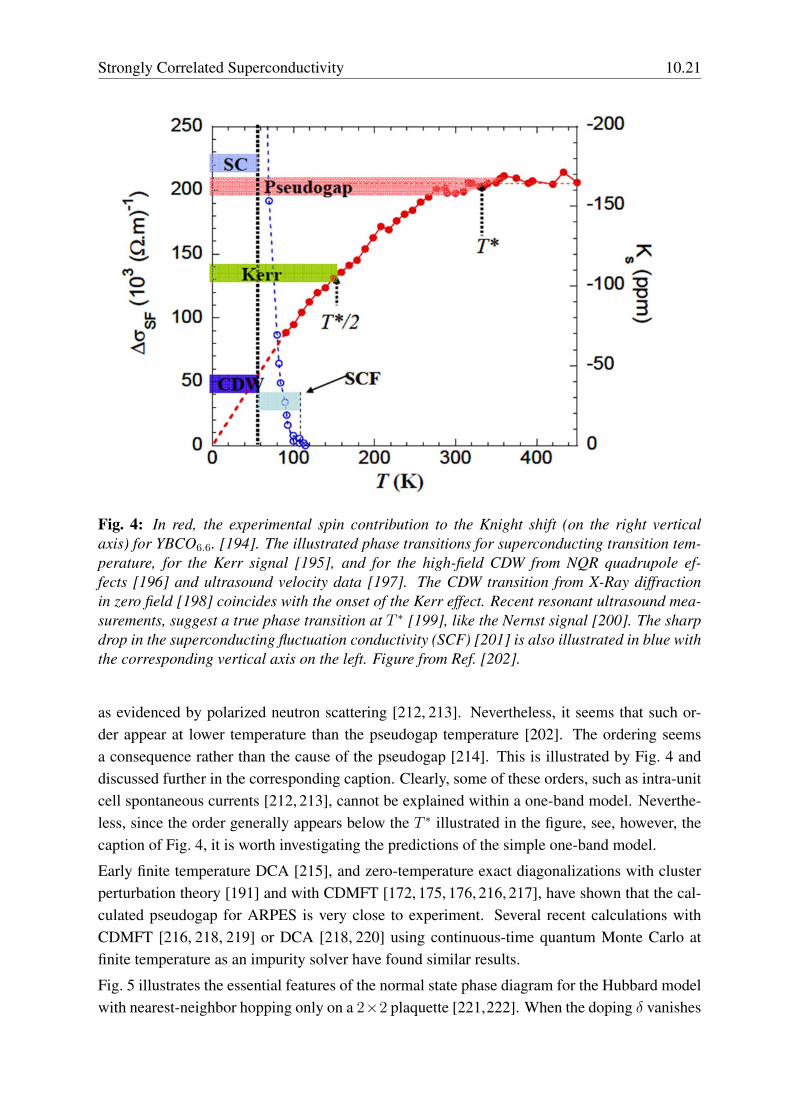
Fig. 4: In red, the experimental spin contribution to the Knight shift (on the right verticalaxis) for YBCO6.6. [194]. The illustrated phase transitions for superconducting transition tem-perature, for the Kerr signal [195], and for the high-field CDW from NQR quadrupole ef-fects [196] and ultrasound velocity data [197]. The CDW transition from X-Ray diffractionin zero field [198] coincides with the onset of the Kerr effect. Recent resonant ultrasound mea-surements, suggest a true phase transition at T ∗ [199], like the Nernst signal [200]. The sharpdrop in the superconducting fluctuation conductivity (SCF) [201] is also illustrated in blue withthe corresponding vertical axis on the left. Figure from Ref. [202].
as evidenced by polarized neutron scattering [212, 213]. Nevertheless, it seems that such or-der appear at lower temperature than the pseudogap temperature [202]. The ordering seemsa consequence rather than the cause of the pseudogap [214]. This is illustrated by Fig. 4 anddiscussed further in the corresponding caption. Clearly, some of these orders, such as intra-unitcell spontaneous currents [212, 213], cannot be explained within a one-band model. Neverthe-less, since the order generally appears below the T
∗ illustrated in the figure, see, however, thecaption of Fig. 4, it is worth investigating the predictions of the simple one-band model.
Early finite temperature DCA [215], and zero-temperature exact diagonalizations with clusterperturbation theory [191] and with CDMFT [172, 175, 176, 216, 217], have shown that the cal-culated pseudogap for ARPES is very close to experiment. Several recent calculations withCDMFT [216, 218, 219] or DCA [218, 220] using continuous-time quantum Monte Carlo atfinite temperature as an impurity solver have found similar results.
Fig. 5 illustrates the essential features of the normal state phase diagram for the Hubbard modelwith nearest-neighbor hopping only on a 2×2 plaquette [221,222]. When the doping δ vanishes
10.22 Andre-Marie S. Tremblay
Correlated metal
PG
(a)
(b)
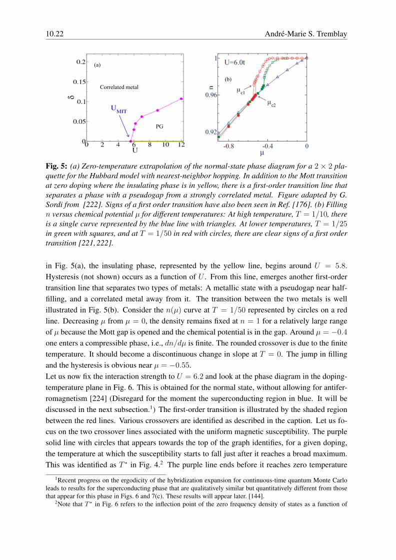
Fig. 5: (a) Zero-temperature extrapolation of the normal-state phase diagram for a 2 × 2 pla-quette for the Hubbard model with nearest-neighbor hopping. In addition to the Mott transitionat zero doping where the insulating phase is in yellow, there is a first-order transition line thatseparates a phase with a pseudogap from a strongly correlated metal. Figure adapted by G.Sordi from [222]. Signs of a first order transition have also been seen in Ref. [176]. (b) Fillingn versus chemical potential µ for different temperatures: At high temperature, T = 1/10, thereis a single curve represented by the blue line with triangles. At lower temperatures, T = 1/25
in green with squares, and at T = 1/50 in red with circles, there are clear signs of a first ordertransition [221, 222].
in Fig. 5(a), the insulating phase, represented by the yellow line, begins around U = 5.8.Hysteresis (not shown) occurs as a function of U . From this line, emerges another first-ordertransition line that separates two types of metals: A metallic state with a pseudogap near half-filling, and a correlated metal away from it. The transition between the two metals is wellillustrated in Fig. 5(b). Consider the n(µ) curve at T = 1/50 represented by circles on a redline. Decreasing µ from µ = 0, the density remains fixed at n = 1 for a relatively large rangeof µ because the Mott gap is opened and the chemical potential is in the gap. Around µ = −0.4
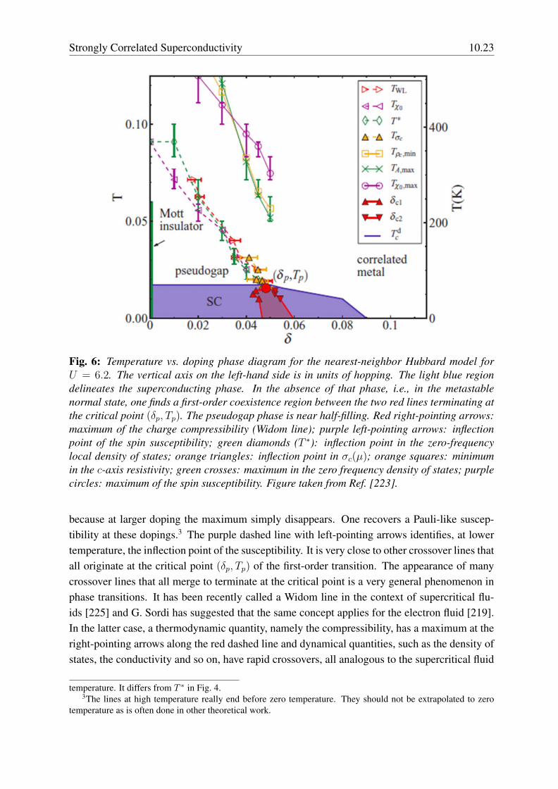
one enters a compressible phase, i.e., dn/dµ is finite. The rounded crossover is due to the finitetemperature. It should become a discontinuous change in slope at T = 0. The jump in fillingand the hysteresis is obvious near µ = −0.55.Let us now fix the interaction strength to U = 6.2 and look at the phase diagram in the doping-temperature plane in Fig. 6. This is obtained for the normal state, without allowing for antifer-romagnetism [224] (Disregard for the moment the superconducting region in blue. It will bediscussed in the next subsection.1) The first-order transition is illustrated by the shaded regionbetween the red lines. Various crossovers are identified as described in the caption. Let us fo-cus on the two crossover lines associated with the uniform magnetic susceptibility. The purplesolid line with circles that appears towards the top of the graph identifies, for a given doping,the temperature at which the susceptibility starts to fall just after it reaches a broad maximum.This was identified as T
∗ in Fig. 4.2 The purple line ends before it reaches zero temperature
1Recent progress on the ergodicity of the hybridization expansion for continuous-time quantum Monte Carloleads to results for the superconducting phase that are qualitatively similar but quantitatively different from thosethat appear for this phase in Figs. 6 and 7(c). These results will appear later. [144].
2Note that T ∗ in Fig. 6 refers to the inflection point of the zero frequency density of states as a function of
Strongly Correlated Superconductivity 10.23
Fig. 6: Temperature vs. doping phase diagram for the nearest-neighbor Hubbard model forU = 6.2. The vertical axis on the left-hand side is in units of hopping. The light blue regiondelineates the superconducting phase. In the absence of that phase, i.e., in the metastablenormal state, one finds a first-order coexistence region between the two red lines terminating atthe critical point (δp, Tp). The pseudogap phase is near half-filling. Red right-pointing arrows:maximum of the charge compressibility (Widom line); purple left-pointing arrows: inflectionpoint of the spin susceptibility; green diamonds (T ∗): inflection point in the zero-frequencylocal density of states; orange triangles: inflection point in σc(µ); orange squares: minimumin the c-axis resistivity; green crosses: maximum in the zero frequency density of states; purplecircles: maximum of the spin susceptibility. Figure taken from Ref. [223].
because at larger doping the maximum simply disappears. One recovers a Pauli-like suscep-tibility at these dopings.3 The purple dashed line with left-pointing arrows identifies, at lowertemperature, the inflection point of the susceptibility. It is very close to other crossover lines thatall originate at the critical point (δp, Tp) of the first-order transition. The appearance of manycrossover lines that all merge to terminate at the critical point is a very general phenomenon inphase transitions. It has been recently called a Widom line in the context of supercritical flu-ids [225] and G. Sordi has suggested that the same concept applies for the electron fluid [219].In the latter case, a thermodynamic quantity, namely the compressibility, has a maximum at theright-pointing arrows along the red dashed line and dynamical quantities, such as the density ofstates, the conductivity and so on, have rapid crossovers, all analogous to the supercritical fluid
temperature. It differs from T ∗ in Fig. 4.3The lines at high temperature really end before zero temperature. They should not be extrapolated to zero
temperature as is often done in other theoretical work.
10.24 Andre-Marie S. Tremblay
case.It is noteworthy that above the crossover line where a c-axis resistivity minimum occurs (orangesquares in Fig. 6), the temperature dependence is almost linear. In that regime, the c-axis resis-tivity can exceed the appropriate version of the Mott-Ioffe-Regel criterion [226]. Also, at zero-temperature in the pseudogap phase, it was demonstrated that very small orthorhombicity leadsto very large conductivity anisotropy in a doped Mott insulator. This called electronic dynamicalnematicity [227]. Such a very large anisotropy is observed experimentally in YBCO [228].From the microcopic point of view, the probability that the plaquette is in a singlet state withfour electrons increases rapidly as temperature decreases, reaching values larger than 0.5 at thelowest temperatures. The inflection point as a function of temperature of the probability for theplaquette singlet coincides with the Widom line [219].From the point of view of this analysis, the pseudogap is a distinct phase, separated from thecorrelated metal by a first-order transition. It is an unstable phase at low temperature since itappears only if we suppress antiferromagnetism and superconductivity. Nevertheless, as in thecase of the Mott transition, the crossovers at high-temperatures are remnants of the first-ordertransition. The phase transition is in the same universality class as the liquid-gas transition. AsU increases, the critical point moves to larger doping and lower temperature. These calculationswere for values of U very close to the Mott transition so that one could reach temperatures lowenough that the first-order transition is visible. Although one sees crossover phenomena up tovery large values of U , the possibility that the first-order transition turns into a quantum criticalpoint cannot be rejected.In summary for this section, one can infer from the plaquette studies that even with antiferro-magnetic correlations that can extend at most to the first-neighbors, one can find a pseudogapand, as I discuss below, d-wave superconductivity. The pseudogap mechanism in this case isclearly related to short-range Mott physics, not to AFM correlation lengths that exceed the ther-mal de Broglie wavelength. Similarly, the pairing comes from the exchange interaction J , butthat does not necessarily mean long wavelength antiferromagnetic correlations.
5.3 Superconducting state
When the interaction U is larger than that necessary to lead to a Mott insulator at half-filling,d-wave superconductivity has many features that are very non-BCS like. That is the topic ofthis section.But first, is there d-wave superconductivity in the one-band Hubbard model or its strong-coupling version, the t-J model? Many-methods suggest that there is [114, 128, 230–232].But there is no unanimity [233]. For reviews, see for example Refs. [74,108,115]. In DCA withlarge clusters and finite-size study, Jarrell’s group has found convincing evidence of d-wavesuperconductivity [145] at U = 4t. This is too small to lead to a Mott insulator at half-fillingbut even for U below the Mott transition there was still sometimes some dispute regarding theexistence of superconductivity. For larger U and 8-site clusters [229] one finds d-wave super-conductivity and a pseudogap. It is remarkable that very similar results were obtained earlier
Strongly Correlated Superconductivity 10.25
with the variational cluster approximation on various size clusters [234–236] and with CDMFTon 2 × 2 plaquettes [172, 216, 224]. With a realistic band-structure, the competition betweensuperconductivity and antiferromagnetism can be studied and the asymmetry between the holeand electron-doped cuprates comes out clearly [172, 234–236].Let us move back to finite temperature results. Fig. 6 shows that the superconducting phaseappears in a region that is not delimited by a dome, as in experiment, but that instead the tran-sition temperature T
dc becomes independent of doping in the pseudogap region [224]. There is
a first-order transition to the Mott insulator at half-filling. One expects that a mean-field treat-ment overestimates the value of T d
c . That transition temperature Tdc in the pseudogap region is
interpreted as the temperature at which local pairs form. This could be the temperature at whicha superconducting gap appears in tunneling experiments [214, 237] without long-range phasecoherence. Many other experiments suggest the formation of local pairs at high temperaturein the pseudogap region [238–242]. Note, however, that T d
c is not the same as the pseudogaptemperature. The two phenomena are distinct [224].It is important to realize the following non-BCS feature of strongly correlated superconductivity.The saturation of T d
c at low temperature occurs despite the fact that the order parameter has adome shape, vanishing as we approach half-filling [172,224]. The order parameter is discussedfurther below. For now, we can ask what is the effect of the size of the cluster on T
dc . Fig. 7(a)
for an 8 site cluster [229] shows that T dc at half-filling is roughly 30% smaller than at optimal
doping, despite the fact that the low temperature superfluid density vanishes at half-filling, asseen in Fig. 7(b). Again, this is not expected from BCS. Since it seems that extremely largeclusters would be necessary to observe a dome shape with vanishing T
dc at infinitesimal doping,
it would be natural to conclude that long wavelength superconducting or antiferromagneticfluctuations are necessary to reproduce the experiment. The long-wavelength fluctuations thatcould be the cause of the decrease of T d
c could be quantum and classical phase fluctuations [243–246], fluctuations in the magnitude of the order parameter [247], or of some competing order,such as antiferromagnetism or a charge-density wave. Evidently, the establishment of long-range order of a competing phase would also be effective [248]. Finally, in the real system,disorder can play a role [249, 250].Another non-BCS feature of strongly correlated superconductivity appears in the single-particledensity of states [224]. Whereas in BCS the density of states is symmetrical near zero frequency,Fig. 7(c) demonstrates that the strong asymmetry present in the pseudogap normal state (dashedred line) survives in the superconducting state. The asymmetry is clearly a property of the Mottinsulator since it is easier to remove an electron (ω < 0) than to add one (ω > 0). Very nearω = 0, all the densities of states in Fig. 7(c) are qualitatively similar since they are dictated bythe symmetry-imposed nodes nodes that are an emergent property of d-wave superconductors.Once the normal state is a correlated metal, for example at doping δ = 0.06, the (particle-hole)symmetry is recovered.The correlated metal leads then to superconducting properties akin to those of spin-fluctuationmediated BCS superconductivity. For example, in the overdoped regime superconductivity dis-appears concomitantly with the low frequency peak of the local spin susceptibility [149]. But in

10.26 Andre-Marie S. Tremblay
(a) (b)
(c)
(d)
Fig. 7: (a) Superconducting critical temperature of the Hubbard model with nearest neighborhopping calculated for U = 6 t using the 8-site DCA [229]. Dashed red line denotes a crossoverto the normal state pseudogap. Dotted blue lines indicate the range of temperatures studied.Note that the temperature axis does not begin at zero. Figure from Ref. [229]. (b) Superfluidstiffness at T = t/60. Figure from Ref. [229]. (c) Low frequency part of the local density ofstates ρ(ω) at U = 6.2t, T = 1/100 for the normal state and the superconducting state (reddashed and blue solid lines). Figure from Ref. [224]. (d) Cumulative order parameter, i.e., theintegral of the anomalous Green function (or Gork’ov function) IF (ω). The dashed green lineis IF (ω) for a d-wave BCS superconductor with a cutoff at ωc = 0.5, which plays the role of theDebye frequency. In that case, the indices i and j in Eq. (23) are near-neighbor. The magentaline is extracted [149] from Eliashberg theory for Pb in Ref. [89]. Frequencies in that caseare measured in units of the transverse phonon frequency, ωT . The scale of the vertical axis isarbitrary. For the s-wave superconductors, one takes i = j in Eq. (23). Figure from Ref. [149].
the underdoped regime, where there is a pseudogap, the difference between the pairing mech-anism in a doped Mott insulator and the pairing mechanism in a doped fluctuating itinerantantiferromagnet comes out very clearly when one takes into account nearest-neighbor repul-sion [90]. Indeed, the doped Mott insulator is much more resilient to near-neighbor repulsionthan a spin-fluctuation mediated BCS superconductor, for reasons that go deep into the natureof superconductivity in a doped Mott insulator. This is an important result that goes much be-yond the mean-field arguments of Eqs. (2) to (5). In this approach, when there is near-neighborrepulsion, one finds that superconductivity should disappear when V > J . In cuprates, taking

Strongly Correlated Superconductivity 10.27
the value of the near-neighbor Coulomb interaction with a relative dielectric constant of order10 we estimate that V , the value of near-neighbor repulsion, is of order V ≈ 400 meV whileJ ≈ 130 meV. So, from the mean-field point of view, superconductivity would not occur in thehole-doped cuprates under such circumstances.To understand the resilience of strongly correlated superconductivity to near-neighbor repulsionV , we need to worry about the dynamics of pairing. To this end, consider the function IF (ω),defined through the integral
IF (ω) = − ω
0
dω
πImF
Rij (ω
) , (23)
where FR is the retarded Gork’ov function (or off-diagonal Green function in the Nambu for-
malism) defined in imaginary time by Fij ≡ −Tci↑(τ)cj↓(0) with i and j nearest-neighbors.The infinite frequency limit of IF (ω) is equal to ci↑cj↓ which in turn is proportional to thed-wave order parameter ψ. As should become clear below, IF (ω) is useful to estimate thefrequencies that are relevant for pair binding. The name “cumulative order parameter” forIF (ω) [90] is suggestive of the physical content of that function.Fig. 7(d) illustrates the behavior of IF (ω) in well known cases. The dashed green line is IF (ω)
for a d-wave BCS superconductor with a cutoff at ωc = 0.5. In BCS theory, that would be theDebye frequency. In BCS then, IF (ω) is a monotonically increasing function of ω that reachesits asymptotic value at the BCS cutoff frequency ωc [149]. The magenta line in Fig. 7(d) isobtained from Eliashberg theory for Pb in Ref. [89]. The two glitches before the maximumcorrespond to the transverse, ωT , and longitudinal, ωL, peaks in the phonon density of states. Inthe Eliashberg approach, which includes a retarded phonon interaction as well as the Coulombpseudopotential µ∗ that represents the repulsive electron-electron interaction [149], the functionovershoots its asymptotic value at frequencies near the main phonon frequencies before decay-ing to its final value. The decrease occurs essentially because of the presence of the repulsiveCoulomb pseudopotantial, as one can deduce [90] from the examples treated in Ref. [89].The resilience of strongly correlated superconductors to near-neighbor repulsion is best illus-trated by Figs. 8(a) to (c). Each panel illustrates the order parameter as a function of doping.The dome shape that we alluded to earlier appears in panels (b) and (c) for U larger than thecritical value necessary to obtain a Mott insulator at half-filling. At weak coupling, U = 4t
in panel (a), the dome shape appears if we allow antiferromagnetism to occur [172]. Panel (a)illustrates the sensitivity of superconductivity to near-neighbor repulsion V at weak coupling.At V/U = 1.5/4 superconductivity has disappeared. By contrast, at strong coupling, U = 8t
in panel (b), one notices that for V twice as large as in the previous case and for the same ratioV/U = 3/8 superconductivity is still very strong. In fact, the order parameter is not very sen-sitive to V in the underdoped regime. Sensitivity to V occurs mostly in the overdoped regime,which is more BCS-like. The same phenomena are observed in panel (c) for U = 16t.To understand the behavior of the order parameter in the strongly correlated case, let us returnto the cumulative order parameter. If we define the characteristic frequency ωF as the frequencyat which the cumulative order parameter reaches half of its asymptotic value, one can check that

10.28 Andre-Marie S. Tremblay
(d)
(e)
(f)
(b)
(c)
Fig. 8: All results for these figures were obtained with CDMFT and the exact diagonalizationsolver with the bath parametrization defined in Ref. [90]. The three panels on the left are forthe d-wave order parameter ψ obtained from the off-diagonal component of the lattice Greenfunction as a function of cluster doping for (a) U = 4t, (b) U = 8t and (c) U = 16t andvarious values of V . The three panels on the right represent the integral of the anomalousGreen function (or Gork’ov function) IF (ω) obtained after extrapolation to η = 0 of ω + iη forseveral values of V at (d) U = 8t, δ = 0.05 (e) U = 8t, δ = 0.2 (f) U = 16t, δ = 0.05 with δ
the value of doping. Frequency is measured in energy units with t = 1. The asymptotic valueof the integral, IF (∞), equal to the order parameter, is shown as horizontal lines. IF (ω) is thecumulative order parameter defined by Eq. (23). The characteristic frequency ωF is defined asthe frequency at which IF (ω) is equal to half of its asymptotic value. The horizontal arrow inpanel (d) indicates how ωF is obtained.
this frequency scales as J . Hence, not only does the optimal value of the order parameter scaleas J , but so does the characteristic frequency over which the order parameter builds up.
The qualitative aspects of the effects of V , are clearer if we focus on the largest value U = 16t
in panel (f) for the underdoped case δ = 0.05. The red curve with filled circles is for V = 0. ForV = 8t, the black curve with open squares shows that the maximum of the cumulative orderparameter is larger by roughly a factor of 2 than for the V = 0 case. This is because at strongcoupling V also contributes to the effective J and thus to attraction at low frequencies. Indeed,in the presence of V , J increases from 4t
2/U at V = 0 to 4t
2/(U − V ). That increase can
be understood by considering two singly-occupied neighboring spins on a square lattice. If allother sites are occupied, the contribution to the potential energy from V is 7V . When one of thetwo electrons is placed on the same site as its neighbor, they together now have three neighbors,hence the potential energy contribution from V is 6V . The energy denominator in second-order degenerate perturbation theory thus becomes U − 7V + 6V = U − V , which explains

Strongly Correlated Superconductivity 10.29
the increased value of J in the presence of V . The ratio of the effective J at U = 16t, V = 8t
to that at U = 16t, V = 0 is U/(U − V ) = 2, which explains the observed increase in themaximum value of IF (ω) by a factor of two. At larger frequencies, however, V is detrimentalto superconductivity, leading to a Coulomb pseudopotential µ∗ that reduces the value of theorder parameter, just as in the case of lead described above. The effect of µ∗ is largest when V
is largest, as expected. Overall, the low-frequency contribution of J to the increase in bindingis compensated by the high-frequency detrimental effect of V .
It is also remarkable that the frequency scale over which the cumulative order parameter reachesits asymptotic value seems to equal a few times J , just as it equals a few times the largest phononfrequency in Fig. 7(d) for the Eliashberg theory of lead. This observation is consistent with thefact that the order parameter reaches its asymptotic value for U = 16t in Fig 8(f) at a frequencyroughly half that where the asymptotic regime is reached for U = 8t in Fig 8(d). Indeed, atV = 0, J is smaller by a factor of two when U increases by a factor of two.
By comparing Fig. 7(d) for the BCS and Eliashberg cases with Fig. 8(e) for the overdoped caseδ = 0.20 and Fig. 8(c) for the underdoped case δ = 0.05, both for U = 8t, one verifies thatthe overdoped case is more BCS-like. This is consistent with the greater sensitivity of the orderparameter to V that one can observe in the overdoped regime of Figs. 8(b) and (c).
Let us end with one of the most striking properties of strongly-correlated superconductivity.Layered organic superconductors of the κ-BEDT family can be modelled by the one-band Hub-bard model on an anisotropic triangular lattice at half-filling [13, 251]. By changing pressure,one can tune the normal state through a Mott transition. The metallic state is at high pressure.At low temperature, pressure changes the insulating state, which can be either antiferromag-netic [11] or spin liquid [252], to a superconducting state with a non s-wave order parameter.See Ref. [253] for a review. One finds experimentally that the superconducting Tc is largest atthe transition, in other words, closest to the insulating phase. In addition, Tc is larger in thecompounds that have the largest mass renormalization in the normal metallic state, i.e., in themost strongly correlated ones [13]. All of this is highly counter-intuitive. I have run out ofspace to explain the theoretical situation on this issue. Let us just remark that at T = 0 withan exact diagonalization solver, one finds with quantum cluster methods [254] that indeed theorder-parameter is largest near the first-order Mott transition [255]. If Tc scales with the orderparameter, this type of approach thus reproduces a counter-intuitive result. The existence ofunconventional superconductivity in the Hubbard model on the anisotropic triangular lattice is,however, disputed [256].
In the model for the cuprates, the value of the order parameter at optimal doping increases withU starting from small U and reaches a maximum at intermediate coupling before decreasingwith J at large U . In other words, as a function of U , the largest value that the order parametercan take is for U ≈ 6t where the Mott transition occurs at half-filling. Analogously, as a func-tion of doping, at U = 6.2, the maximum Tc occurs near the critical doping for the pseudogapto correlated metal transition [224].
10.30 Andre-Marie S. Tremblay
6 ConclusionProgress with numerical methods, especially cluster generalizations of DMFT, has shown inrecent years that much of the physics of strongly correlated superconductors is contained in theone-band Hubbard model. Confidence in the method comes from extensive benchmarking, andfrom the agreement at intermediate coupling with TPSC, which is also benchmarked and validup to intermediate coupling. The fact that both the cuprates and the layered organics are welldescribed gives additional confidence in the validity of the approach. Much physical insight canbe gained by these methods. In the future, it will be useful to use them to discriminate betweenthe various versions of mean-field theories based on slave-particle approaches. A mean-fieldapproach that would contain most of the features of numerical approaches might help us togain further insight into the problem. Variational wave functions, even if treated with numericalmethods, are also helpful to this end.Much remains to be done. In the one-band model, it is necessary to develop methods thatallow us to reliably investigate long-wavelength instabilities, such as the CDW observed forthe cuprates. Investigating theoretically all the details of the highly unusual superconductingproperties of the layered organics also remains to be done. And the description of all featuresof the cuprates at lower temperature calls for even more extensive studies of the three-bandmodel [115, 257–259].
AcknowledgmentsI am especially grateful to David Senechal, Giovanni Sordi, Patrick Semon, Dominic Bergeron,Yury Vilk, Bumsoo Kyung, Kristjan Haule and to many other collaborators on some of thework discussed above, including V. Bouliane, M. Capone, A. Day, M. Civelli, B. Davoudi,S. Kancharla, G. Kotliar, J.-S. Landry, P.-L. Lavertu, M.-A. Marois, S. Roy. This work waspartially supported by the Tier I Canada Research Chair Program (A.-M.S.T.) by CFI, MELS,Calcul Quebec and Compute Canada.

Strongly Correlated Superconductivity 10.31
References[1] J.H. de Boer and E.J.W. Verwey, Proceedings of the Physical Society 49, 59 (1937)
[2] M. Imada, A. Fujimori, and Y. Tokura, Rev. Mod. Phys. 70, 1039 (1998)
[3] F. Steglich, J. Aarts, C.D. Bredl, W. Lieke, D. Meschede, W. Franz, and H. Schafer,Physical Review Letters 43, 1892 (1979)
[4] D. Jerome, A. Mazaud, M. Ribault, and K. Bechgaard, J. Phys. Lett. 41, L95 (1980)
[5] J. Bednorz and K. Muller, Z. Phys. B 64, 189 (1986)
[6] J. Williams, A.J. Schultz, U. Geiser, K.D. Carlson, A.M. Kini, H. Wang, W.K. Kwok,M.-H. Whangbo, and J.E. Schriber, Science 252, 1501 (1991)
[7] D. Jerome, Science 252, 1509 (1991)
[8] Y. Kamihara, T. Watanabe, M. Hirano, and H. Hosono,J. Am. Chem. Soc. 130, 3296 (2008)
[9] H. Ito, T. Ishiguro, M. Kubota, and G. Saito, J. Phys. Soc. Japan 65, 2987 (1996)
[10] K. Kanoda, Physica C: Superconductivity 282-287. part 1, 299 (1997)
[11] S. Lefebvre, P. Wzietek, S. Brown, C. Bourbonnais, D. Jerome, C. Meziere,M. Fourmigue, and P. Batail, Phys. Rev. Lett. 85, 5420 (2000)
[12] P. Limelette, P. Wzietek, S. Florens, A. Georges, T.A. Costi, C. Pasquier, D. Jerome,C. Meziere, and P. Batail, Phys. Rev. Lett. 91, 016401 (2003)
[13] B.J. Powell and R.H. McKenzie, J. Phys. Cond. Mat. 18, R827 (2006)
[14] J. Hubbard, Proc. Roy. Soc. London A 276, 238 (1963)
[15] J. Kanamori, Prog. Theor. Phys. 30, 275 (1963)
[16] M.C. Gutzwiller, Phys. Rev. Lett. 10, 159 (1963)
[17] P. Nozieres and J.M. Luttinger, Phys. Rev. 127, 1423 (1962)
[18] J.M. Luttinger and P. Nozieres, Phys. Rev. 127, 1431 (1962)
[19] A.B. Harris and R.V. Lange, Phys. Rev. 157, 295 (1967)
[20] W. Metzner, Phys. Rev. B 43, 8549 (1991)
[21] M. Bartkowiak and K.A. Chao, Phys. Rev. B 46, 9228 (1992)
[22] S. Pairault, D. Senechal, and A.-M.S. Tremblay, Phys. Rev. Lett. 80, 5389 (1998)
10.32 Andre-Marie S. Tremblay
[23] S. Pairault, D. Senechal, and A.-M.S. Tremblay, Eur. Phys. J. B 16, 85 (2000)
[24] C. Gros, R. Joynt, and T.M. Rice, Phys. Rev. B 36, 381 (1987)
[25] P.W. Anderson, Phys. Rev. 115, 2 (1959)
[26] P.W. Anderson, Science 235, 1196 (1987)
[27] M.B.J. Meinders, H. Eskes, and G.A. Sawatzky, Phys. Rev. B 48, 3916 (1993)
[28] P.W. Anderson, Science 177, 393 (1972)
[29] R.B. Laughlin: A Different Universe: Reinventing Physics from the Bottom Down(Basic Books, 2006)
[30] D. Pines: Emergent Behavior in Quantum Matter (2010)http://www.learner.org/courses/physics/unit/text.html?
unit=8&secNum=0
[31] A. Reymbaut, unpublished (2013)
[32] N.D. Mermin and H. Wagner, Phys. Rev. Lett. 17, 1133 (1966)
[33] P.C. Hohenberg, Phys. Rev. 158, 383 (1967)
[34] G. Toulouse, Commun. Phys. (1977)
[35] A. Georges and G. Kotliar, Phys. Rev. B 45, 6479 (1992)
[36] M. Jarrell, Phys. Rev. Lett. 69, 168 (1992)
[37] A. Georges, G. Kotliar, W. Krauth, and M.J. Rozenberg, Rev. Mod. Phys. 68, 13 (1996)
[38] J.R. Schrieffer, X.G. Wen, and S.C. Zhang: Phys. Rev. B 39, 11663 (1989)
[39] J.D. Reger and A.P. Young, Phys. Rev. B 37, 5978 (1988)
[40] D. Vaknin, S.K. Sinha, D.E. Moncton, D.C. Johnston, J.M. Newsam, C.R. Safinya, andH.E. King, Phys. Rev. Lett. 58, 2802 (1987)
[41] M. Takahashi, J. Phys. C: Solid State Physics 10, 1289 (1977)
[42] A.H. MacDonald, S.M. Girvin, and D. Yoshioka, Phys. Rev. B 37, 9753 (1988)
[43] J.-Y.P. Delannoy, M.J.P. Gingras, P.C.W. Holdsworth, and A.-M.S. Tremblay,Phys. Rev. B 72, 115114 (2005)
[44] H.-Y. Yang, A.M. Lauchli, F. Mila, and K.P. Schmidt,Phys. Rev. Lett. 105, 267204 (2010)
Strongly Correlated Superconductivity 10.33
[45] B. Dalla Piazza, M. Mourigal, M. Guarise, H. Berger, T. Schmitt, K.J. Zhou, M. Grioni,and H.M. Rønnow, Phys. Rev. B 85, 100508 (2012)
[46] T. Holstein and H. Primakoff, Phys. Rev. 58, 1098 (1940)
[47] A.V. Chubukov and S. Sachdev, Phys. Rev. Lett. 71, 169 (1993)
[48] F.D.M. Haldane, Phys. Rev. Lett. 50, 1153 (1983)
[49] A.W. Sandvik: Lecture notes for course given at the 14th Training Course in Physics ofStrongly Correlated Systems, Salerno (Vietri sul Mare, Italy, October 2009)http://arxiv.org/abs/1101.3281
[50] M. Campostrini, M. Hasenbusch, A. Pelissetto, P. Rossi, and E. Vicari,Phys. Rev. B 65, 144520 (2002)
[51] E. Kozik, E. Burovski, V.W. Scarola, and M. Troyer, Phys. Rev. B 87, 205102 (2013)
[52] N. Prokof’ev, B. Svistunov, and I. Tupitsyn, Phys. Lett. A 238, 253 (1998)
[53] M. Boninsegni, N.V. Prokof’ev, and B.V. Svistunov, Phys. Rev. E 74, 036701 (2006)
[54] S. Sorella, Phys. Rev. B 71, 241103 (2005)
[55] T. Giamarchi and C. Lhuillier, Phys. Rev. B 43, 12943 (1991)
[56] E. Manousakis, Rev. Mod. Phys. 63, 1 (1991)
[57] http://pitp.physics.ubc.ca/confs/sherbrooke/archives.html
[58] http://pitp.physics.ubc.ca/confs/sherbrooke2012/archives.
html
[59] S. Chakravarty, B.I. Halperin, and D.R. Nelson, Phys. Rev. B 39, 2344 (1989)
[60] B. Keimer, N. Belk, R. J. Birgeneau, A. Cassanho, C.Y. Chen, M. Greven, M.A. Kastner,A. Aharony, Y. Endoh, R.W. Erwin, and G. Shirane, Phys. Rev. B 46, 14034 (1992)
[61] P. Monthoux and D. Pines, Phys. Rev. B 47, 6069 (1993)
[62] T. Moriya: Spin Fluctuations in Itinerant Electron Magnetism(Springer, Heidelberg, 1985)
[63] N.E. Bickers, D.J. Scalapino, and S.R. White, Phys. Rev. Lett. 62, 961 (1989)
[64] N.E. Bickers and D.J. Scalapino, Ann. Phys. (USA) 193, 206 (1989)
[65] D. Zanchi and H.J. Schulz, Phys. Rev. B 61, 13609 (2000)

10.34 Andre-Marie S. Tremblay
[66] C. Honerkamp, M. Salmhofer, N. Furukawa, and T.M. Rice,Phys. Rev. B 63, 035109 (2001)
[67] R. Shankar, Rev. Mod. Phys. 66, 129 (1994)
[68] R.K. Kaul, M.A. Metlitski, S. Sachdev, and C. Xu, Phys. Rev. B 78, 045110 (2008)
[69] S. Sachdev, M.A. Metlitski, Y. Qi, and C. Xu, Phys. Rev. B 80, 155129 (2009)
[70] Y.M. Vilk and A.-M.S. Tremblay, J. Phys I (France) 7, 1309 (1997)
[71] S. Allen, A.-M.S. Tremblay, and Y.M. Vilk, in D. Senechal, C. Bourbonnais, and A.-M.S. Tremblay (eds.): Theoretical Methods for Strongly Correlated Electrons (2003)
[72] A. M. S. Tremblay: Two-Particle-Self-Consistent Approach for the Hubbard Modelin F. Mancini and A. Avella (eds.): Strongly Correlated Systems (Springer, 2011)
[73] N. Bulut, D.J. Scalapino, and S.R. White, Phys. Rev. Lett. 73, 748 (1994)
[74] A. M.S. Tremblay, B. Kyung, and D. Senechal, Low Temp. Phys. 32, 424 (2006)
[75] K.A. Brueckner, T. Soda, P.W. Anderson, and P. Morel, Phys. Rev. 118, 1442 (1960)
[76] Y. M. Vilk and A.-M.S. Tremblay, J. Phys. Chem. Solids (UK) 56, 1769 (1995)
[77] Y. M. Vilk and A.-M.S. Tremblay, Europhys. Lett. 33, 159 (1996)
[78] S. Moukouri, S. Allen, F. Lemay, B. Kyung, D. Poulin, Y.M. Vilk, and A.-M.S. Tremblay,Phys. Rev. B 61, 7887 (2000)
[79] E.M. Motoyama, G. Yu, I.M. Vishik, O.P. Vajk, P.K. Mang, and M. Greven,Nature 445, 186 (2007)
[80] B. Kyung, V. Hankevych, A.-M. Dare, and A.-M.S. Tremblay,Phys. Rev. Lett. 93, 147004 (2004)
[81] D. Bergeron, D. Chowdhury, M. Punk, S. Sachdev, and A.-M.S. Tremblay,Phys. Rev. B 86, 155123 (2012)
[82] C.M. Varma, J. Low Temp. Phys. 126, 901 (2002)
[83] P.A. Lee, Phys. Rev. Lett. 71, 1887 (1993)
[84] L. Taillefer, B. Lussier, R. Gagnon, K. Behnia, and H. Aubin,Phys. Rev. Lett. 79, 483 (1997)
[85] G.M. Eliashberg, Soviet Phys. JETP 11, 696 (1960)
[86] J.P. Carbotte, Rev. Mod. Phys. 62, 1027 (1990)

Strongly Correlated Superconductivity 10.35
[87] F. Marsiglio and J. Carbotte, arXiv:cond-mat/0106143 (2001)
[88] J.R. Schrieffer: Theory of Superconductivity (W.A. Benjamin, New York, 1964)
[89] D.J. Scalapino, J.R. Schrieffer, and J W. Wilkins, Phys. Rev. 148, 263 (1966)
[90] D. Senechal, A.G.R. Day, V. Bouliane, and A.-M.S. Tremblay,Phys. Rev. B 87, 075123 (2013)
[91] N.E. Hussey, K. Takenaka, and H. Takagi, Phil. Mag. 84, 2847 (2004)
[92] M. Gurvitch and A.T. Fiory, Phys. Rev. Lett. 59, 1337 (1987)
[93] O. Gunnarsson, M. Calandra, and J.E. Han, Rev. Mod. Phys. 75, 1085 (2003)
[94] D. Bergeron, V. Hankevych, B. Kyung, and A.-M.S. Tremblay,Phys. Rev. B 84, 085128 (2011)
[95] W. Xu, K. Haule, and G. Kotliar: arXiv:1304.7486 (2013)
[96] P.A. Lee, N. Nagaosa, and X.-G. Wen, Rev. Mod. Phys. 78, 17 (2006)
[97] S.D. Obertelli, J.R. Cooper, and J.L. Tallon, Phys. Rev. B 46, 14928 (1992)
[98] T. Honma and P. H. Hor, Phys. Rev. B 77, 184520 (2008)
[99] Y. Ando, Y. Kurita, S. Komiya, S. Ono, and K. Segawa,Phys. Rev. Lett. 92, 197001 (2004)
[100] D.C. Peets, D.G. Hawthorn, K.M. Shen, Y.-J. Kim, D.S. Ellis, H. Zhang, S. Komiya,Y. Ando, G.A. Sawatzky, R. Liang, D. A. Bonn, and W.N. Hardy,Phys. Rev. Lett. 103, 087402 (2009)
[101] P. Phillips and M. Jarrell, Phys. Rev. Lett. 105, 199701 (2010)
[102] C.T. Chen, F. Sette, Y. Ma, M.S. Hybertsen, E.B. Stechel, W.M.C. Foulkes, M. Schulter,S.-W. Cheong, A.S. Cooper, L.W. Rupp, B. Batlogg, Y.L. Soo, Z.H. Ming, A. Krol, andY.H. Kao, Phys. Rev. Lett. 66, 104 (1991)
[103] K. Miyake, S. Schmitt-Rink, and C.M. Varma, Phys. Rev. B 34, 6554 (1986)
[104] G. Kotliar and J. Liu, Phys. Rev. Lett. 61, 1784 (1988)
[105] P.W. Anderson, P.A. Lee, M. Randeria, T.M. Rice, N. Trivedi, and F.C. Zhang,J. Phys.: Condensed Matter 16, R755 (2004)
[106] W. Kohn and J.M. Luttinger, Phys. Rev. Letters 15, 524 (1965)
[107] J. Mraz and R. Hlubina, Phys. Rev. B 67, 174518 (2003)
10.36 Andre-Marie S. Tremblay
[108] S. Maiti and A.V. Chubukov: arXiv:1305.4609 (2013)
[109] S. Raghu, S.A. Kivelson, and D.J. Scalapino, Phys. Rev. B 81, 224505 (2010)
[110] M.T. Beal-Monod, C. Bourbonnais, and V.J. Emery, Phys. Rev. B 34, 7716 (1986)
[111] D.J. Scalapino, J. Loh, E., and J.E. Hirsch, Phys. Rev. B 34, 8190 (1986)
[112] M.R. Norman, M. Randeria, B. Janko, and J.C. Campuzano,Phys. Rev. B 61, 14742 (2000)
[113] T. Moriya and K. Ueda, Rep. Prog. Phys. 66, 1299 (2003)
[114] P. Monthoux, D. Pines, and G.G. Lonzarich, Nature 450, 1177 (2007)
[115] D.J. Scalapino: Physica C 470, S1 (2010)
[116] S.R. Hassan, B. Davoudi, B. Kyung, and A.-M.S. Tremblay,Phys. Rev. B 77, 094501 (2008)
[117] D.M. Broun, Nat Phys 4, 170 (2008)
[118] S. Sachdev, physica status solidi (b) 247, 537 (2010)
[119] N. Doiron-Leyraud and L. Taillefer, Physica C 481, 161 (2012)
[120] L.G. Caron and C. Bourbonnais Physica B & C 143, 453 (1986)
[121] C. Bourbonnais and A. Sedeki, Phys. Rev. B. in press (2012)
[122] C. Bourbonnais, Mol. Crys. Liq. Crys. 119, 11 (1985)
[123] C. Bourbonnais, in C.B. Dou and J. Zinn-Justin (eds.) Les Houches 1991, Session LVI:Strongly interacting fermiions and high Tc superconductivity (Elsevier, 1995), pp. 307
[124] C.J. Halboth and W. Metzner, Phys. Rev. Lett. 85, 5162 (2000)
[125] M. Salmhofer, C. Honerkamp, W. Metzner, and O. Lauscher,Prog. Theor. Phys. 112, 943 (2004)
[126] W. Metzner, M. Salmhofer, C. Honerkamp, V. Meden, and K. Schonhammer,Rev. Mod. Phys. 84, 299 (2012)
[127] B. Kyung, J.-S. Landry, and A.-M.S. Tremblay, Phys. Rev. B 68, 174502 (2003)
[128] S. Nishiyama, K. Miyake, and C. Varma, cond-mat/1302.2160v1 (2013)
[129] N. Doiron-Leyraud, P. Auban-Senzier, S. Rene de Cotret, C. Bourbonnais, D. Jerome,K. Bechgaard, and L. Taillefer, Phys. Rev. B 80, 214531 (2009)

Strongly Correlated Superconductivity 10.37
[130] Y. Zhang, E. Demler, and S. Sachdev, Phys. Rev. B 66, 094501 (2002)
[131] S.-X. Yang, H. Fotso, S.-Q. Su, D. Galanakis, E. Khatami, J.-H. She, J. Moreno,J. Zaanen, and M. Jarrell, Phys. Rev. Lett. 106, 047004 (2011)
[132] S.E. Barnes, J. Phys. F 6, 1375 (1976)
[133] P. Coleman, Phys. Rev. B 29, 3035 (1984)
[134] G. Kotliar and A.E. Ruckenstein, Phys. Rev. Lett. 57, 1362 (1986)
[135] D. Yoshida, J. Phys. Soc. Japan 58, 32 (1989)
[136] C. Jayaprakash, H.R. Krishnamurthy, and S. Sarker, Phys. Rev. B 40, 2610 (1989)
[137] S. Florens and A. Georges, Phys. Rev. B 66, 165111 (2002)
[138] S.R. Hassan and L. de’ Medici, Phys. Rev. B 81, 035106 (2010)
[139] P. Phillips, Rev. Mod. Phys. 82, 1719 (2010).
[140] D. Boies, F. A. Jackson, and T. A. M. S., Int. J. Mod. Phys. B 9, 1001 (1995)
[141] K.-Y. Yang, T.M. Rice, and F.-C. Zhang, Phys. Rev. B 73, 174501 (2006)
[142] E. Schachinger and J.P. Carbotte, Phys. Rev. B 81, 014519 (2010)
[143] J.P.F. LeBlanc, J.P. Carbotte, and E.J. Nicol, Phys. Rev. B 83, 184506 (2011)
[144] P.Semon and G. Sordi, unpublished (2013)
[145] T.A. Maier, M. Jarrell, T.C. Schulthess, P.R.C. Kent, and J.B. White,Phys. Rev. Lett. 95, 237001 (2005)
[146] M. Inui, S. Doniach, P.J. Hirschfeld, and A.E. Ruckenstein, Phys. Rev. B 37, 2320 (1988)
[147] P.W. Anderson, Science 316, 1705 (2007)
[148] T.A. Maier, D. Poilblanc, and D.J. Scalapino, Phys. Rev. Lett. 100, 237001 (2008)
[149] B. Kyung, D. Senechal, and A.-M.S. Tremblay, Phys. Rev. B 80, 205109 (2009)
[150] D.J. Scalapino, Physics Reports 250, 329 (1995)
[151] A. Avela and F. Mancini: The Composite Operator Method (COM)in F. Mancini and A. Avella (eds.): Strongly Correlated Systems (Springer, 2011)
[152] M.H. Hettler, A.N. Tahvildar-Zadeh, M. Jarrell, T. Pruschke, and H.R. Krishnamurthy,Phys. Rev. B 58, R7475 (1998)

10.38 Andre-Marie S. Tremblay
[153] G. Kotliar, S. Y. Savrasov, G. Palsson, and G. Biroli, Phys. Rev. Lett. 87, 186401 (2001)
[154] A.I. Lichtenstein and M.I. Katsnelson, Phys. Rev. B 62, R9283 (2000)
[155] T. Maier, M. Jarrell, T. Pruschke, and M.H. Hettler, Rev. Mod. Phys. 77, 1027 (2005)
[156] G. Kotliar, S.Y. Savrasov, K. Haule, V.S. Oudovenko, O. Parcollet, and C.A. Marianetti,Rev. Mod. Phys. 78, 865 (2006)
[157] W. Metzner and D. Vollhardt, Phys. Rev. Lett. 62, 324 (1989)
[158] M. Potthoff, M. Aichhorn, and C. Dahnken, Phys. Rev. Lett. 91, 206402 (2003)
[159] M. Potthoff, Eur. Phys. J. B 36, 335 (2003)
[160] M. Potthoff, Eur. Phys. J. B 32, 429 (2003)
[161] M. Potthoff: Self-Energy-Functional Theoryin F. Mancini and A. Avella (eds.): Strongly Correlated Systems (Springer, 2011)
[162] T.D. Stanescu, M. Civelli, K. Haule, and G. Kotliar: Ann. Phys. 321, 1682 (2006)
[163] D. Senechal: In D. Senechal (ed.) High Performance Computing Systems and Applica-tions and OSCAR symposium (2003)
[164] T. D. Stanescu and G. Kotliar: Phys. Rev. B 70, 205112 (2004)
[165] S. Sakai, G. Sangiovanni, M. Civelli, Y. Motome, K. Held, and M. Imada,Phys. Rev. B 85, 035102 (2012)
[166] Th. Maier, M. Potthoff and D. Senechal, unpublished
[167] G. Biroli and G. Kotliar, Phys. Rev. B 65, 155112 (2002)
[168] K. Aryanpour, T.A. Maier, and M. Jarrell, Phys. Rev. B 71, 037101 (2005)
[169] G. Biroli and G. Kotliar, Phys. Rev. B 71, 037102 (2005)
[170] B. Kyung, G. Kotliar, and A.-M.S. Tremblay, Phys. Rev. B 73, 205106 (2006)
[171] M. Caffarel and W. Krauth, Phys. Rev. Lett. 72, 1545 (1994)
[172] S.S. Kancharla, B. Kyung, D. Senechal, M. Civelli, M. Capone, G. Kotliar, andA.-M.S. Tremblay, Phys. Rev. B 77, 184516 (2008)
[173] M. Capone, M. Civelli, S.S. Kancharla, C. Castellani, and G. Kotliar,Phys. Rev. B 69, 195105 (2004)
[174] M. Civelli: Investigation of strongly correlated electron system with cellular dynamicalmean-field theory. (Ph.D. thesis, Rutgers University, 2006)
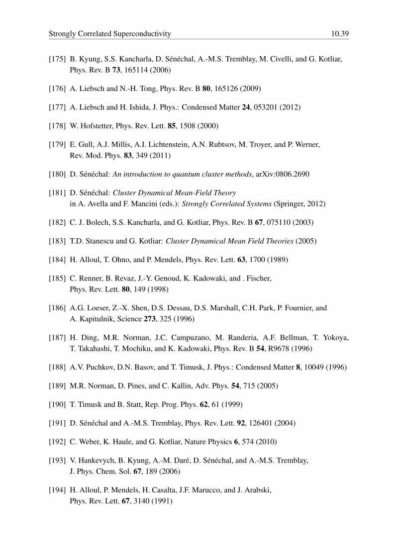
Strongly Correlated Superconductivity 10.39
[175] B. Kyung, S.S. Kancharla, D. Senechal, A.-M.S. Tremblay, M. Civelli, and G. Kotliar,Phys. Rev. B 73, 165114 (2006)
[176] A. Liebsch and N.-H. Tong, Phys. Rev. B 80, 165126 (2009)
[177] A. Liebsch and H. Ishida, J. Phys.: Condensed Matter 24, 053201 (2012)
[178] W. Hofstetter, Phys. Rev. Lett. 85, 1508 (2000)
[179] E. Gull, A.J. Millis, A.I. Lichtenstein, A.N. Rubtsov, M. Troyer, and P. Werner,Rev. Mod. Phys. 83, 349 (2011)
[180] D. Senechal: An introduction to quantum cluster methods, arXiv:0806.2690
[181] D. Senechal: Cluster Dynamical Mean-Field Theoryin A. Avella and F. Mancini (eds.): Strongly Correlated Systems (Springer, 2012)
[182] C. J. Bolech, S.S. Kancharla, and G. Kotliar, Phys. Rev. B 67, 075110 (2003)
[183] T.D. Stanescu and G. Kotliar: Cluster Dynamical Mean Field Theories (2005)
[184] H. Alloul, T. Ohno, and P. Mendels, Phys. Rev. Lett. 63, 1700 (1989)
[185] C. Renner, B. Revaz, J.-Y. Genoud, K. Kadowaki, and . Fischer,Phys. Rev. Lett. 80, 149 (1998)
[186] A.G. Loeser, Z.-X. Shen, D.S. Dessau, D.S. Marshall, C.H. Park, P. Fournier, andA. Kapitulnik, Science 273, 325 (1996)
[187] H. Ding, M.R. Norman, J.C. Campuzano, M. Randeria, A.F. Bellman, T. Yokoya,T. Takahashi, T. Mochiku, and K. Kadowaki, Phys. Rev. B 54, R9678 (1996)
[188] A.V. Puchkov, D.N. Basov, and T. Timusk, J. Phys.: Condensed Matter 8, 10049 (1996)
[189] M.R. Norman, D. Pines, and C. Kallin, Adv. Phys. 54, 715 (2005)
[190] T. Timusk and B. Statt, Rep. Prog. Phys. 62, 61 (1999)
[191] D. Senechal and A.-M.S. Tremblay, Phys. Rev. Lett. 92, 126401 (2004)
[192] C. Weber, K. Haule, and G. Kotliar, Nature Physics 6, 574 (2010)
[193] V. Hankevych, B. Kyung, A.-M. Dare, D. Senechal, and A.-M.S. Tremblay,J. Phys. Chem. Sol. 67, 189 (2006)
[194] H. Alloul, P. Mendels, H. Casalta, J.F. Marucco, and J. Arabski,Phys. Rev. Lett. 67, 3140 (1991)
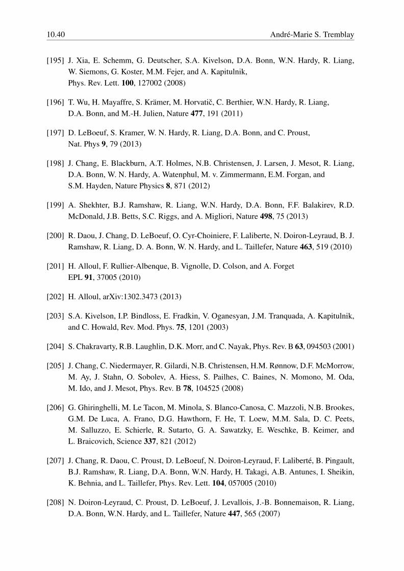
10.40 Andre-Marie S. Tremblay
[195] J. Xia, E. Schemm, G. Deutscher, S.A. Kivelson, D.A. Bonn, W.N. Hardy, R. Liang,W. Siemons, G. Koster, M.M. Fejer, and A. Kapitulnik,Phys. Rev. Lett. 100, 127002 (2008)
[196] T. Wu, H. Mayaffre, S. Kramer, M. Horvatic, C. Berthier, W.N. Hardy, R. Liang,D.A. Bonn, and M.-H. Julien, Nature 477, 191 (2011)
[197] D. LeBoeuf, S. Kramer, W. N. Hardy, R. Liang, D.A. Bonn, and C. Proust,Nat. Phys 9, 79 (2013)
[198] J. Chang, E. Blackburn, A.T. Holmes, N.B. Christensen, J. Larsen, J. Mesot, R. Liang,D.A. Bonn, W. N. Hardy, A. Watenphul, M. v. Zimmermann, E.M. Forgan, andS.M. Hayden, Nature Physics 8, 871 (2012)
[199] A. Shekhter, B.J. Ramshaw, R. Liang, W.N. Hardy, D.A. Bonn, F.F. Balakirev, R.D.McDonald, J.B. Betts, S.C. Riggs, and A. Migliori, Nature 498, 75 (2013)
[200] R. Daou, J. Chang, D. LeBoeuf, O. Cyr-Choiniere, F. Laliberte, N. Doiron-Leyraud, B. J.Ramshaw, R. Liang, D. A. Bonn, W. N. Hardy, and L. Taillefer, Nature 463, 519 (2010)
[201] H. Alloul, F. Rullier-Albenque, B. Vignolle, D. Colson, and A. ForgetEPL 91, 37005 (2010)
[202] H. Alloul, arXiv:1302.3473 (2013)
[203] S.A. Kivelson, I.P. Bindloss, E. Fradkin, V. Oganesyan, J.M. Tranquada, A. Kapitulnik,and C. Howald, Rev. Mod. Phys. 75, 1201 (2003)
[204] S. Chakravarty, R.B. Laughlin, D.K. Morr, and C. Nayak, Phys. Rev. B 63, 094503 (2001)
[205] J. Chang, C. Niedermayer, R. Gilardi, N.B. Christensen, H.M. Rønnow, D.F. McMorrow,M. Ay, J. Stahn, O. Sobolev, A. Hiess, S. Pailhes, C. Baines, N. Momono, M. Oda,M. Ido, and J. Mesot, Phys. Rev. B 78, 104525 (2008)
[206] G. Ghiringhelli, M. Le Tacon, M. Minola, S. Blanco-Canosa, C. Mazzoli, N.B. Brookes,G.M. De Luca, A. Frano, D.G. Hawthorn, F. He, T. Loew, M.M. Sala, D. C. Peets,M. Salluzzo, E. Schierle, R. Sutarto, G. A. Sawatzky, E. Weschke, B. Keimer, andL. Braicovich, Science 337, 821 (2012)
[207] J. Chang, R. Daou, C. Proust, D. LeBoeuf, N. Doiron-Leyraud, F. Laliberte, B. Pingault,B.J. Ramshaw, R. Liang, D.A. Bonn, W.N. Hardy, H. Takagi, A.B. Antunes, I. Sheikin,K. Behnia, and L. Taillefer, Phys. Rev. Lett. 104, 057005 (2010)
[208] N. Doiron-Leyraud, C. Proust, D. LeBoeuf, J. Levallois, J.-B. Bonnemaison, R. Liang,D.A. Bonn, W.N. Hardy, and L. Taillefer, Nature 447, 565 (2007)
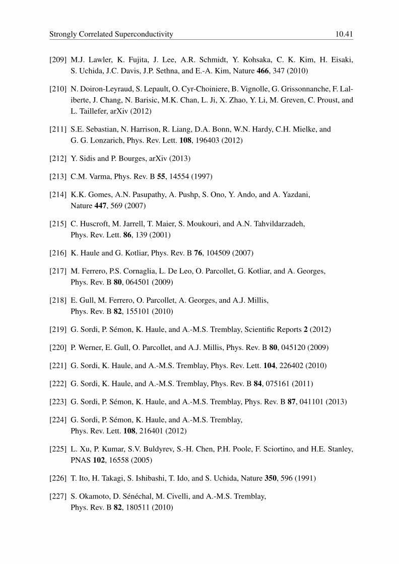
Strongly Correlated Superconductivity 10.41
[209] M.J. Lawler, K. Fujita, J. Lee, A.R. Schmidt, Y. Kohsaka, C. K. Kim, H. Eisaki,S. Uchida, J.C. Davis, J.P. Sethna, and E.-A. Kim, Nature 466, 347 (2010)
[210] N. Doiron-Leyraud, S. Lepault, O. Cyr-Choiniere, B. Vignolle, G. Grissonnanche, F. Lal-iberte, J. Chang, N. Barisic, M.K. Chan, L. Ji, X. Zhao, Y. Li, M. Greven, C. Proust, andL. Taillefer, arXiv (2012)
[211] S.E. Sebastian, N. Harrison, R. Liang, D.A. Bonn, W.N. Hardy, C.H. Mielke, andG. G. Lonzarich, Phys. Rev. Lett. 108, 196403 (2012)
[212] Y. Sidis and P. Bourges, arXiv (2013)
[213] C.M. Varma, Phys. Rev. B 55, 14554 (1997)
[214] K.K. Gomes, A.N. Pasupathy, A. Pushp, S. Ono, Y. Ando, and A. Yazdani,Nature 447, 569 (2007)
[215] C. Huscroft, M. Jarrell, T. Maier, S. Moukouri, and A.N. Tahvildarzadeh,Phys. Rev. Lett. 86, 139 (2001)
[216] K. Haule and G. Kotliar, Phys. Rev. B 76, 104509 (2007)
[217] M. Ferrero, P.S. Cornaglia, L. De Leo, O. Parcollet, G. Kotliar, and A. Georges,Phys. Rev. B 80, 064501 (2009)
[218] E. Gull, M. Ferrero, O. Parcollet, A. Georges, and A.J. Millis,Phys. Rev. B 82, 155101 (2010)
[219] G. Sordi, P. Semon, K. Haule, and A.-M.S. Tremblay, Scientific Reports 2 (2012)
[220] P. Werner, E. Gull, O. Parcollet, and A.J. Millis, Phys. Rev. B 80, 045120 (2009)
[221] G. Sordi, K. Haule, and A.-M.S. Tremblay, Phys. Rev. Lett. 104, 226402 (2010)
[222] G. Sordi, K. Haule, and A.-M.S. Tremblay, Phys. Rev. B 84, 075161 (2011)
[223] G. Sordi, P. Semon, K. Haule, and A.-M.S. Tremblay, Phys. Rev. B 87, 041101 (2013)
[224] G. Sordi, P. Semon, K. Haule, and A.-M.S. Tremblay,Phys. Rev. Lett. 108, 216401 (2012)
[225] L. Xu, P. Kumar, S.V. Buldyrev, S.-H. Chen, P.H. Poole, F. Sciortino, and H.E. Stanley,PNAS 102, 16558 (2005)
[226] T. Ito, H. Takagi, S. Ishibashi, T. Ido, and S. Uchida, Nature 350, 596 (1991)
[227] S. Okamoto, D. Senechal, M. Civelli, and A.-M.S. Tremblay,Phys. Rev. B 82, 180511 (2010)
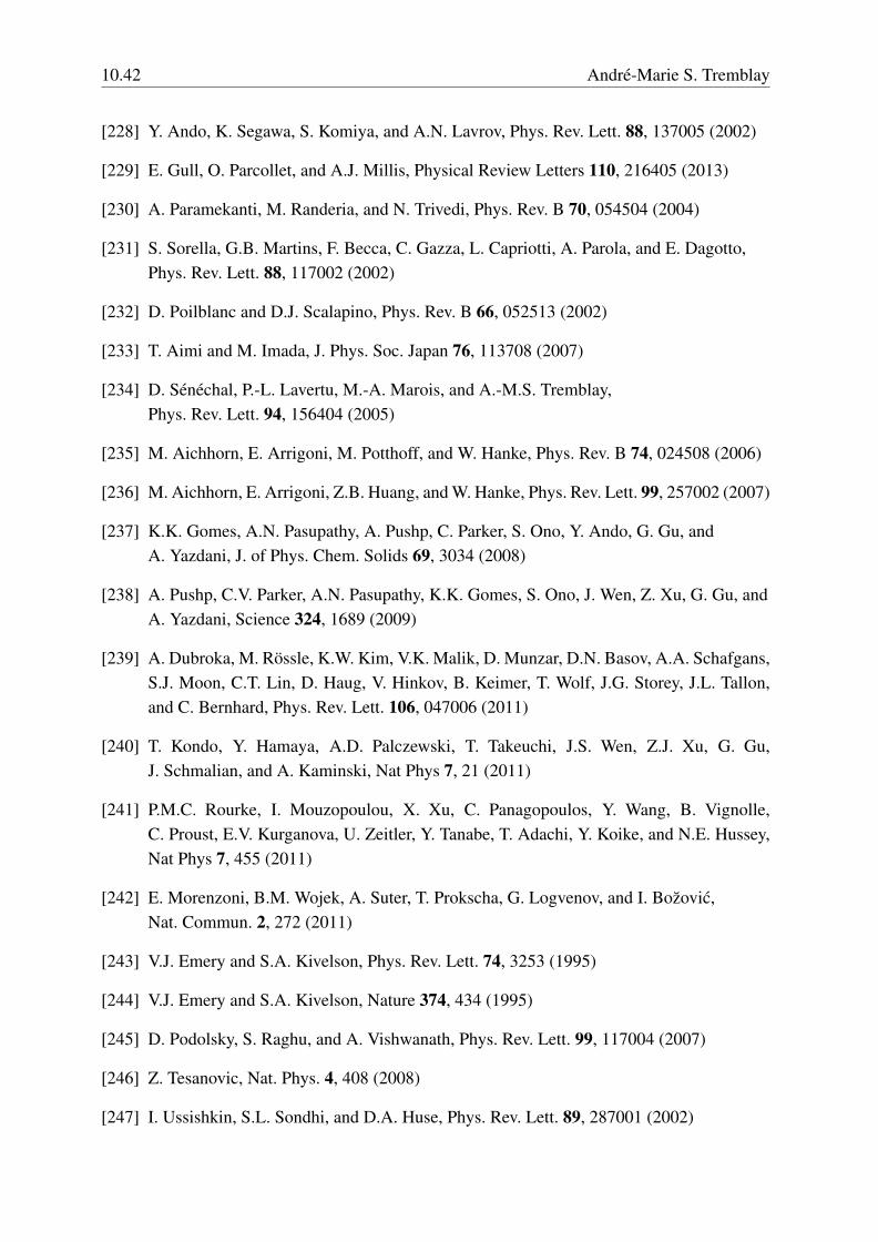
10.42 Andre-Marie S. Tremblay
[228] Y. Ando, K. Segawa, S. Komiya, and A.N. Lavrov, Phys. Rev. Lett. 88, 137005 (2002)
[229] E. Gull, O. Parcollet, and A.J. Millis, Physical Review Letters 110, 216405 (2013)
[230] A. Paramekanti, M. Randeria, and N. Trivedi, Phys. Rev. B 70, 054504 (2004)
[231] S. Sorella, G.B. Martins, F. Becca, C. Gazza, L. Capriotti, A. Parola, and E. Dagotto,Phys. Rev. Lett. 88, 117002 (2002)
[232] D. Poilblanc and D.J. Scalapino, Phys. Rev. B 66, 052513 (2002)
[233] T. Aimi and M. Imada, J. Phys. Soc. Japan 76, 113708 (2007)
[234] D. Senechal, P.-L. Lavertu, M.-A. Marois, and A.-M.S. Tremblay,Phys. Rev. Lett. 94, 156404 (2005)
[235] M. Aichhorn, E. Arrigoni, M. Potthoff, and W. Hanke, Phys. Rev. B 74, 024508 (2006)
[236] M. Aichhorn, E. Arrigoni, Z.B. Huang, and W. Hanke, Phys. Rev. Lett. 99, 257002 (2007)
[237] K.K. Gomes, A.N. Pasupathy, A. Pushp, C. Parker, S. Ono, Y. Ando, G. Gu, andA. Yazdani, J. of Phys. Chem. Solids 69, 3034 (2008)
[238] A. Pushp, C.V. Parker, A.N. Pasupathy, K.K. Gomes, S. Ono, J. Wen, Z. Xu, G. Gu, andA. Yazdani, Science 324, 1689 (2009)
[239] A. Dubroka, M. Rossle, K.W. Kim, V.K. Malik, D. Munzar, D.N. Basov, A.A. Schafgans,S.J. Moon, C.T. Lin, D. Haug, V. Hinkov, B. Keimer, T. Wolf, J.G. Storey, J.L. Tallon,and C. Bernhard, Phys. Rev. Lett. 106, 047006 (2011)
[240] T. Kondo, Y. Hamaya, A.D. Palczewski, T. Takeuchi, J.S. Wen, Z.J. Xu, G. Gu,J. Schmalian, and A. Kaminski, Nat Phys 7, 21 (2011)
[241] P.M.C. Rourke, I. Mouzopoulou, X. Xu, C. Panagopoulos, Y. Wang, B. Vignolle,C. Proust, E.V. Kurganova, U. Zeitler, Y. Tanabe, T. Adachi, Y. Koike, and N.E. Hussey,Nat Phys 7, 455 (2011)
[242] E. Morenzoni, B.M. Wojek, A. Suter, T. Prokscha, G. Logvenov, and I. Bozovic,Nat. Commun. 2, 272 (2011)
[243] V.J. Emery and S.A. Kivelson, Phys. Rev. Lett. 74, 3253 (1995)
[244] V.J. Emery and S.A. Kivelson, Nature 374, 434 (1995)
[245] D. Podolsky, S. Raghu, and A. Vishwanath, Phys. Rev. Lett. 99, 117004 (2007)
[246] Z. Tesanovic, Nat. Phys. 4, 408 (2008)
[247] I. Ussishkin, S.L. Sondhi, and D.A. Huse, Phys. Rev. Lett. 89, 287001 (2002)

Strongly Correlated Superconductivity 10.43
[248] E. Fradkin, S.A. Kivelson, M.J. Lawler, J.P. Eisenstein, and A.P. Mackenzie,Annual Review of Condensed Matter Physics 1, 153 (2010)
[249] F. Rullier-Albenque, H. Alloul, F. Balakirev, and C. Proust, EPL 81, 37008 (2008)
[250] H. Alloul, J. Bobroff, M. Gabay, and P.J. Hirschfeld, Rev. Mod. Phys. 81, 45 (2009)
[251] H. Kino and H. Fukuyama: J. Phys. Soc. Japan 65, 2158 (1996)
[252] Y. Shimizu, K. Miyagawa, K. Kanoda, M. Maesato, and G. Saito,Phys. Rev. Lett. 91, 107001 (2003)
[253] B.J. Powell and R.H. McKenzie, Rep. Prog. Phys. 74, 056501 (2011)
[254] P. Sahebsara and D. Senechal, Phys. Rev. Lett. 97, 257004 (2006)
[255] B. Kyung, G. Kotliar, and A.-M.S. Tremblay, Phys. Rev. B 73, 205106 (2006)
[256] S. Dayal, R.T. Clay, and S. Mazumdar, Phys. Rev. B 85, 165141 (2012)
[257] V.J. Emery, Phys. Rev. Lett. 58, 2794 (1987)
[258] A. Macridin, T.A. Maier, M.S. Jarrell, and G.A. Sawatzky,Phys. Rev. B 71, 134527 (2005)
[259] W. Hanke, M. Kiesel, M. Aichhorn, S. Brehm, and E. Arrigoni,Eur. Phys. J. 188, 15 (2010)


![Strongly Correlated Superconductivity · Strongly Correlated Superconductivity 10.5 occupation number that defines the Fermi surface. This is the Landau Fermi liquid [17,18]. Emergent](https://img.dokumen.tips/doc/110x75/5eb5d8e916c37935a563db58/strongly-correlated-superconductivity-strongly-correlated-superconductivity-105.jpg)