Strategic Consumer Response to Dynamic Pricing of Perishable Products

Minho Cho · Ming Fan · Yong-Pin Zhou§ Department of Information Systems and Operations Management

Michael G. Foster School of Business, University of Washington, Seattle, WA 98195-3200

mc9@u.washington.edu · mfan@u.washington.edu · yongpin@u.washington.edu

August 2008

Abstract

Dynamic pricing is a standard practice that sellers use for revenue management. With the vast

availability of pricing and inventory data on the Internet, it is possible for consumers to become

aware of the pricing strategies used by sellers and to develop strategic responses. In this paper,

we study the strategic response of consumers to dynamic prices for perishable products. As price

fluctuates with the changes in time and inventory, a strategic consumer may choose to postpone a

purchase in anticipation of lower prices in the future. We analyze a threshold purchasing policy

for the strategic consumer, and conduct numerical studies to study its impact on both the

strategic consumer’s benefits and the seller’s revenue. We find that in most cases the policy can

benefit both the strategic consumer and the seller. In practice, the seller could encourage

consumers waiting by adopting a target price purchasing system.

1. Introduction

Pricing has been an age-old management issue, especially for perishable products facing

uncertain demand. Under the common fixed-price scheme, if the price is set too low, potential

revenue will be lost; but if the price is set too high, demand will be low and perishable products

§ Corresponding author. (Phone) 1-206-221-5324 (Fax) 1-206-543-3968.

2

may be wasted when they expire. Revenue management (a.k.a. yield management) has become

an increasingly popular management tool in selling perishable products. It is widely used not

only in the hospitality industry (e.g. airlines, hotels, and cruise lines), but also in many other

industries where products or capacity are perishable (e.g., golf course reservation, natural gas

pipeline reservation, concert and ball game ticket sales, and fashion products). A detailed review

on the subject was provided by McGill and van Ryzin (1999). Essentially, revenue management

is a method that aims to sell the right inventory unit to the right consumer, at the right time, and

for the right price (Kimes 1989). This is mainly achieved through dynamic pricing and inventory

allocation. More recently, sellers begin to take advantage of the Internet to sell perishable

products online (Choi and Kimes 2002, Liddle 2003). To many sellers, the Internet offers a new

opportunity to implement revenue management techniques such as dynamic pricing because

price changes are easy, inexpensive, and potentially more effective.

Most of the research on revenue management focuses on developing optimal pricing and

inventory allocation policies (e.g. Littlewood 1972, Belobaba 1989, Gallego and van Ryzin

1994, Zhao and Zheng 2000). These models generally assume that consumers are non-forward-

looking and will purchase the products when the prices are below their reservation values. In

contrast, this paper examines how, by looking forward, consumers can strategically respond to

the seller’s dynamic prices over time. The growing use of the Internet provides an opportunity

for consumers to gather information on sellers’ pricing policies and respond strategically. Since

price variation for consumer products on the Internet is high, comparison-shopping can provide

real benefits. The primary online shopping tools that consumers use today are shopbots that do

price comparisons (Montgomery et al. 2004). Traditional shopbots compare prices spatially by

checking the prices at various websites at roughly the same time. They do not anticipate possible

3

future price changes. More recently, researchers have shown interests in developing shopbots

that can also compare prices temporally. One example is the “Hamlet” program1 that studies past

trends in the variation of airline fares and establishes the patterns, which can then be used to

decide whether the consumer should make a purchase immediately or wait for possible future

price reductions (Etzioni et al. 2003). Many critics doubt the effectiveness and the accuracy of

Hamlet's prediction, however, because the underlying factors that determine the prices are not

clearly understood (Knapp 2003).

In this research, we examine the behavior of strategic consumers who responds to

dynamic prices by timing the purchase. The tradeoff is clear: Since the price of a perishable

product changes continuously over time, there is a chance to get the same product at a lower

price by waiting. On the other hand, there is a chance that the product, which is available and

affordable now, may be sold out or become more expensive later if the strategic consumer waits.

We develop a threshold purchasing policy that balances this tradeoff, and examine its impact on

both the consumer and the seller. Focusing on the main factors that influence price, our

analytical approach gives simple and effective solutions, and allows us to derive insights. Using

simulation we also find that the strategic consumer delay could benefit both the consumer and

the seller. This conclusion is closely related to the reservation option used by the seller in

Elmaghraby et al. (2009) which shows the seller can benefit from allowing a strategic customer

who delays his/her purchase to reserve the item (the consumer must purchase the item if its

prices drops to a lower, previously agreed-upon sales price).

It should be noted that in most existing models, while consumer purchasing patterns can

be strategic, their arrivals patterns are usually assumed exogenous. In Biyalorgorsky (2009), the

1 This led to the recent establishment of the website http://farecast.com.

4

author present a model in which the customer can decide strategically to show up or not,

depending on the offering price. It is shown that the seller can use contingent pricing to influence

consumers to show up at the desired time and improve his/her own profit.

The rest of the paper is organized as follows. In the next section, we provide a brief

review of the related literature. In Section 3, we derive a threshold policy that helps a single

strategic consumer to decide when to purchase. In Section 4, we use simulations to evaluate its

benefit to both the strategic consumer and the seller. In Section 5, we examine extensions to our

base model. We make concluding remarks in Section 6.

2. Literature Review

There is an extensive body of literature on revenue management, mostly in the context of airline

ticket sales. For a comprehensive review, see Talluri and van Ryzin (2004). Two different

approaches complement each other. The first assumes that consumers can be categorized into

different classes (e.g. leisure and business travelers) and focuses the analysis on the allocation of

capacity among these classes. Based on the demand forecast for each consumer class, a “booking

limit” of perishable products (e.g. airplane tickets) is computed for each consumer type. These

thresholds can vary over time as demand unfolds (Littlewood 1972, Brumelle and McGill 1993,

Robinson 1995). Literature on capacity allocation usually assumes a monopoly market structure

with the exception that Netessine and Shumsky (2005) analyze seat allocation under both

horizontal and vertical competitions using a game theoretical model. The second approach in

revenue management focuses more on the dynamic pricing aspect of revenue management.

Gallego and van Ryzin (1994) analyze the dynamic pricing policy for one type of product and

homogeneous consumers. The consumers arrive randomly and their valuations for the product

are also random. Important monotonicity properties are derived for the seller’s optimal pricing

5

policy. Zhao and Zheng (2000) extend this model to include non-homogeneous demand.

Consumers are time sensitive so their reservation price distribution may change over time. None

of these models consider consumers’ reaction to the seller’s pricing strategy, however. In their

review of dynamic pricing models, Bitran and Caldentey (2003) point out “incorporating

rationality on the behavior of consumers” as an interesting field of research.

Rather than assuming consumers are price takers, some marketing researchers have

studied rational shopper behavior in the face of random price variations. In Ho, Tang and Bell’s

rational shopper model (1998), the seller chooses one of a finite set of pricing scenarios and

rational shoppers react by purchasing more when the price is low and less when the price is high.

They find, among other things, that when price variability is high, the rational shoppers shop

more frequently and buy fewer units every time. The type of product under consideration is the

daily consumer product, which needs to be purchased and consumed repeatedly and continually

over time. Consequently the main tradeoff for a rational shopper is between the purchase costs

and the inventory holding costs. This differs from the one-time purchase of perishable products,

which is the focus of this paper. Moreover, the price variation in Ho, Tang and Bell (1998) is

random, while the price variation in our paper follows certain optimally determined curves that

are given in the revenue management literature.

Besanko and Winston (1990) study a game between a monopolist, who sets prices for a

new product over time, and strategic consumers, who decide whether to purchase now for the

sure utility or postpone the purchase so as to maximize the future expected utility. In the

equilibrium, the monopolist systematically reduces price over time. Elmaghraby et al. (2005)

also study a game where the seller changes price over time and the buyers submit the desired

quantities at any given price. Liu and van Ryzin (2005) study a similar problem in a discrete

6

time-period setting, and allow consumers to be risk averse. All three papers are based on the

assumption that all consumers are present at the beginning of the game, which results in certain

monotonicity properties. In our paper, consumers arrive randomly over time. Therefore, the

optimal price trajectory depends on the realization of the consumer arrival process, and it may

experience gradual decrease over time and sudden increase right after a purchase is made.

Aviv and Pazgal (2003) also study the strategic consumer reaction to price variations, and

allow consumers to arrive over time. When forward-looking consumers have information about

future price discounts, they may decide to postpone their purchases to a later time when

discounts are offered. In their model, there are only a pre-fixed number of price changes, and the

price-setting seller announces the prices and the price change times ahead of time. While this

may represent a retail-type environment, it does not apply to the situations where the seller

continuously changes its price in response to the realization of stochastic demands. In addition,

in Aviv and Pazgal (2003), the consumers’ valuations are homogeneous and decrease over time

according to a deterministic function known to the seller. Thus, a consumer who arrives at a

certain time will have a deterministic valuation for the product. In contrast, our model assumes

heterogeneous consumer valuations and random consumer arrivals. Consequently, the prices

consumers face are also stochastic.

Anderson and Wilson (2003) study consumer reactions to the dynamic allocation of

airline seats to various fare classes. When all the low-price fares are closed, consumers may

decide to wait before purchasing a ticket in the hope that a low-price fare class will reopen. The

paper does not model consumer behavior explicitly, however.

The model in our paper is most closely related to the dynamic pricing model in Gallego

and van Ryzin (1994). Gallego and van Ryzin (1994) assume that all consumers are price-takers:

7

those who can afford the price purchase right away and those who can’t, leave. In our model,

strategic consumers are patient and would not purchase until the desired time or price of the

product is reached. We are interested in the effect of such a strategy on the consumers’ utility

and the seller’s total revenue.

3. Strategic Consumer Behavior 3.1. Dynamic Pricing Model

We assume that the seller’s pricing strategy follows that in Gallego and van Ryzin (1994), which

we call the GVR model. Therefore, we begin with a brief review of the GVR model. There is a

fixed number, n, of one type of perishable product to be sold during a finite time horizon T. The

product is perishable so all units left at the end of the sales period are worth nothing2. Let k

denote the number of products left, 0 k n≤ ≤ , and t the time units left in the sale horizon,

0 t T≤ ≤ . As is the convention, t gets smaller as time goes by. Therefore, the state of the system

can be described by the vector ),( tk .

Consumer purchases follow a price-sensitive Poisson process. That is, if price is p, then

the instantaneous Poisson arrival rate is ( )pλ , where ( )pλ is decreasing in p and lim 0( )p

pλ→∞

= .

There is another way to interpret this consumer arrival process: Let the arrival of all potential

consumers follow a Poisson process with a constant rate (0)λ . Moreover, let each consumer’s

valuation of the product, v, have the cumulative probability distribution (CDF) ( )( ) 1(0)pF p λ

λ= − .

Thus, when the price is p , an arriving consumer can afford the product with the probability of

2 It will be straightforward to include an end-of-horizon salvage value for each unsold unit.

8

1 ( )F p− . Consequently, the price-sensitive purchase arrival process is Poisson with the

instantaneous rate [ ](0) 1 ( ) ( )F p pλ λ− = . In this paper, the second interpretation will be used.

In any state (k,t), the seller chooses the best price p - or equivalently λ(p) - to maximize

its total expected revenue J(k,t). No inventory holding cost is considered for the seller, which is

standard in the one-period problem setting. Gallego and van Ryzin (1994) show that J(k,t) is

determined by the following equation, with boundary conditions J(n,0)=0 and J(0,t)=0:

( )[ ] ,0 ,1 ,),1(),()(sup),(>∀≥∀−−−=

∂∂ tntkJtkJp

ttkJ λλλ

λ

where p(λ) is the inverse function of λ(p).

The seller’s dynamic pricing strategy is thus summarized in a pricing function ( , )p k t .

Clearly, it is reasonable to expect the price to be higher when fewer units are left, or when more

time is left. Thus, ( , )p k t is decreasing in k but increasing in t . Those properties are proved in

Gallego and van Ryzin (1994).

In the GVR model, all consumers are price takers, which we call regular consumers. In

this paper, we assume there are two types of consumers: regular consumers (RC) and strategic

consumers (SC). To begin with, in this section and next we will assume that there is only one SC

in the system and analyze his/her behavior. In Section 5, we study the extension of having

multiple SCs in the system.

We assume that the SC, with the help of software agents, is able to collect information

about the seller’s pricing policy ( , )p k t and the demand arrival function ( )pλ , and use them to

optimize the timing of her purchase.

The SC exhibits two major differences in her behavior from that of a RC. First, when a

RC cannot afford the item, she simply leaves. In contrast, an SC chooses to wait so that, if the

9

price drops later, she may afford it. Second, when a RC can afford the item at the current price,

she purchases right away. In contrast, an SC may decide to postpone the purchase so that she

may purchase the product at a lower price later.

3.2. Threshold Purchasing Policy

When the SC arrives to find the system in state ( ,k t ), the decision for her is whether to purchase

at the current price ( , )p k t or to wait. If she decides to wait, then what is the desired time or price

level to make the purchase? We study the following two policies:

THRESHOLD TIME POLICY (TTP). With k products available, purchase if and only if there are kt

time units or less left in the sales time horizon, i.e. purchase if and only if kt t≤ .

THRESHOLD PRICE POLICY (TPP). With k products available, purchase if and only if the price is

below a certain threshold price level kp .

Since the SC knows that the seller changes price dynamically, waiting a little bit to

purchase may result in a lower price. How long she waits will have to depend on both the

number of units left, k, and the time left, t. This results in the TTP. From another perspective,

the SC waits till a target price is reached, which is the TPP. Below, we show that the two

policies are equivalent. All proofs of in this paper are shown in the Appendix.

PROPOSITION 1. The threshold price policy (TPP) is equivalent to the threshold time policy

(TTP).

All of the proofs in this paper are provided in the appendix.

Because the TTP and the TPP are equivalent, in this paper we will use them

interchangeably.

10

If the SC arrives with little time but many products left (i.e., small t and big k), the price

may already be lower than her target price kp so the SC will purchase right away. In other

situations, the SC may wait. Clearly, during the wait, it is possible that another consumer may

arrive and make a purchase. In this case, k becomes 1k − , and the SC will continue to follow

the above policies and wait for 1kt − (or 1kp − ).

Now we study how the SC determines the kt s and kp s. Let her have a valuation of v for

the product. The objective for her is to maximize her utility, which is defined to be the difference

between v and the price paid for the product. Clearly, the SC will only purchase the product if the

price is no more than v (i.e., no negative utility). If the SC ends up unable to purchase the

product because the price is higher than v, we say that the consumer receives a utility of 0.

At any time, if the price is below the SC’s valuation, she has two options: purchase now

and get the sure utility, or wait till later to either get the product at a lower price or see the price

jump due to other consumers’ purchases. The SC must carefully balance the consequences of the

two options. We let the threshold tk be the point at which the SC is indifferent between

purchasing now and waiting a little longer. That the threshold tks are such indifference points is

intuitive. Moreover, due to bounded rationality, it is reasonable to assume that the strategic

consumer only considers these two options. A more rigorous approach would also consider the

option of waiting to purchase at a more distant future time. In this case, although we believe the

following proposition still holds, we can only prove it for some special cases. Even when one

considers Equation (1) to be a heuristic, our simulations in Section 4 show it is very effective.

PROPOSITION 2. Let kt be the solution to

{ } ( )

( , )min ( 1, ), ( , ) .

( , )

p k ttp k t v p k tp k tλ

∂∂− = + (1)

11

If kt t≥ , the strategic consumer will purchase right away; and if tk < t, the strategic consumer

will wait and the target purchase time is kt .3.3. Exponential Valuation of the Consumers

Equation (1) can be used to derive the thresholds for any given price strategy p(k,t). To evaluate

its efficiency, we will apply it to the case in which v follows an exponential distribution. This is

the same distribution used in Kincaid and Darling (1963) and Gallego and van Ryzin (1994).

Let the arrival of potential consumers follow a Poisson process with a constant rate of a.

Each consumer’s valuation of the product, v, follows an exponential distribution with a rate of

α . Consequently, when the price is ( , )p k t , the probability that an arriving consumer has a

valuation v higher than ( , )p k t is ( , )p k te α− . Hence, the price-sensitive Poisson arrival rate is

( , )( ( , )) p k tp k t ae αλ −= . For simplicity of notation, α is set to one.

Under these assumptions, Gallego and van Ryzin (1994) show that the optimal pricing

policy for the seller satisfies:

( , ) ( , ) ( 1, ) 1p k t J k t J k t= − − + (2)

where ( , )J k t is the maximum revenue function for the seller and it satisfies:

( , ) ( , )J k t k tt

λ∂=

∂ (3)

and

0

1( , ) log ( ) .!

ki

i

atJ k te i=

⎛ ⎞= ⎜ ⎟⎝ ⎠∑ (4)

In what follows, we will further characterize these functions and derive properties that

will simplify the analysis of Equation (1). To streamline the exposition, we will use ( ),k tλ

instead of ( )( , )p k tλ , and define ( )

( , )

( , ) ( , ),

p k ttg k t p k t

k tλ

∂∂= + . We prove the following results:

12

LEMMA 1. ( )

( , )

( , ),

p k ttp k t

k tλ

∂∂+ is increasing in t.

LEMMA 2. ( )

( , )

( 1, ) ( , ),

p k ttp k t p k t

k tλ

∂∂− > + .

Based on Lemmas 1 and 2, we can find the optimal purchasing thresholds.

PROPOSITION 3. (i) The kt s for the TTP are solutions to ( )

( , )

( , ) .,

p k ttv p k t

k tλ

∂∂= +

(ii) A unique finite solution, kt , exists for every k if and only if 1v ≥ .

Proposition 3 reduces the computational effort for the time thresholds and facilitates

further theoretical analysis. It also has a simple interpretation: When the SC decides not to

purchase right now, two things are possible: the price may go up if another consumer arrives and

the effect of this is [ ]( , ) ( 1, ) ( , )k t p k t p k tλ − − ; or if there is no other arrivals then the price will

gradually go down over time and the effect of this is ( , )p k tt

∂∂

. Proposition 3 shows that the first,

price-jump effect always exceeds the second, time effect.

Therefore, if v is very high, the SC will always purchase immediately. However, the

existence of a finite v limits the first effect, and makes the waiting option more attractive. One

can also easily deduce that the lower the v, the more restrictions it puts on the price-jump effect,

and the consumer is more willing to wait. The properties of the TTP are formally stated in

Proposition 4.

13

PROPOSITION 4. The solution of the TTP has the following properties:

(i) The tks are increasing in v.

(ii) The tks are decreasing in a.

Intuitively speaking, when v is small, the utility for the SC is small if she purchases the

product right away; so the SC has little to lose if she waits and other RCs make purchases (and

the price goes above v), but she has much to gain if the price keeps dropping. On the other hand,

the SC with a higher v will have a higher loss if the price jumps if she waits; but her gain from

waiting for a lower price remains the same as that with a lower v. As a result, the SC with a

higher v will purchase earlier. Numerically, this holds true especially for 1k = . For 1k > , the tks

are quite insensitive to v.

Proposition 4 also states that the bigger the arrival rate a, the smaller the tk. This means

that if the product is “hot,” then the consumer will want to wait longer. This seems counter-

intuitive at first, but it makes sense after a careful examination. When the demand rate is high,

the seller also knows it. As a result, for the same k and t, the price will be higher for a higher a.

Therefore the utility to gain for a consumer with a fixed v is lower. The SC’s risk of losing this

current utility by waiting is smaller now (since a is larger). So the consumer is willing to wait

longer.

When the SC follows the TTP, she needs to estimate the following three parameters to

determine her time thresholds:

• t , the time left

• k , the number of products left

• a, the arrival rate

14

In general, while t is usually easy to estimate, k may not be. If it is a physical item on

display in retail stores, the consumers can check the level of inventory. On the other hand, if the

product is not a physical item (e.g. air ticket), it may be difficult to obtain the seller’s inventory

information. However, sellers are increasingly volunteering such inventory information on their

website and making it easier for consumers to find3. Hence, here we assume consumers can

obtain the inventory level information. In Section 5, we relax this assumption and examine a

policy that does not rely on the sellers’ inventory information.

For the arrival rate a, we prove in the following proposition that when a consumer

follows the TPP, there is no need to estimate that parameter at all:

PROPOSITION 5. The solution to the TPP, kp , is independent of a.

From the proof we see that the pks are independent of a and the tks depend on a only

through the product kat . This makes sense because what’s important for the SC at time t, for a

fixed inventory level k, is not the arrival rate of other consumers, but rather the expected number

of other consumers who will arrive later. This is the product of the arrival rate and how much

time is left, at.

That the threshold prices can be determined with only k and t makes the TPP a lot easier

to use. Also, it is worth noting that the use of the TPP is quite similar to that of the limit order in

stock trading: a consumer arrives to find the current prevailing market price and decides to

transact later when a threshold price is reached. We will have more discussion on this later.

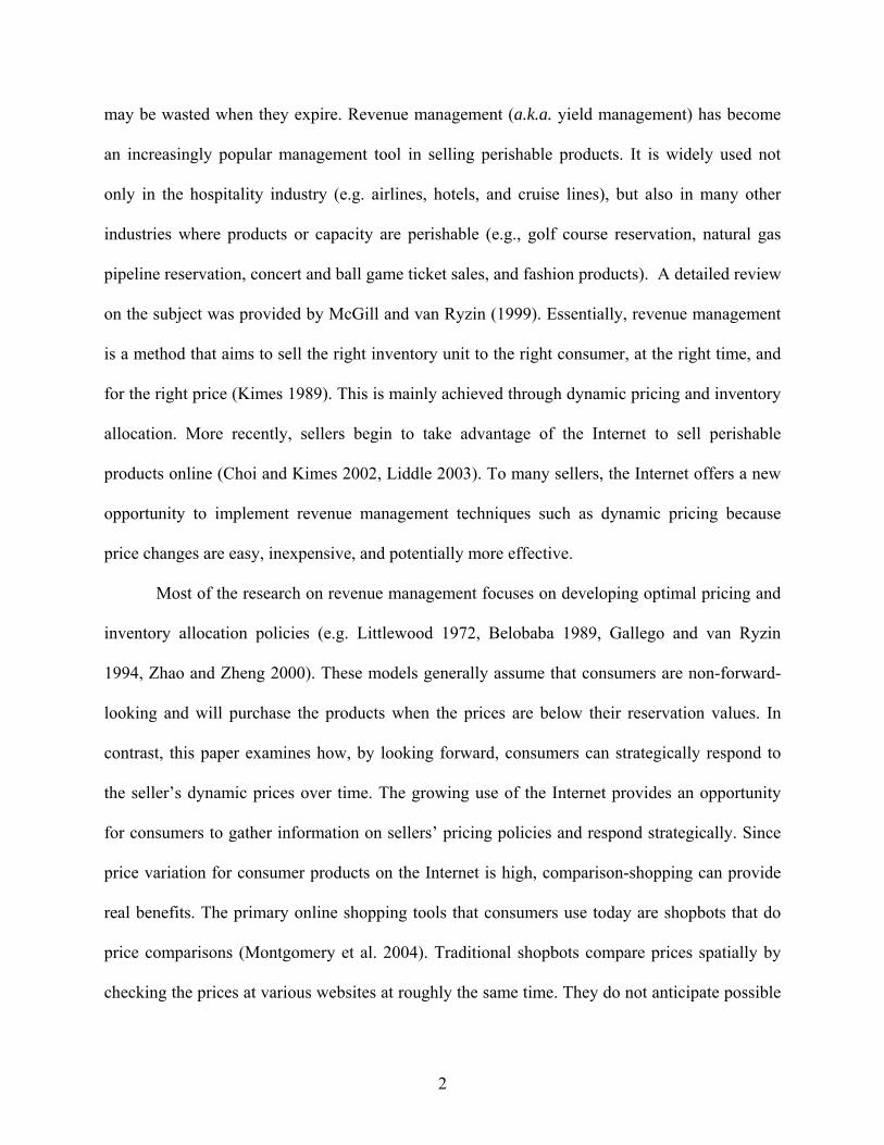
The example in Figure 1 illustrates how the threshold policy works for the SC. Numerical

results show that the threshold policy uses a different threshold time (tk) for each inventory level

3 For example, AA.com, expedia.com, and Travelocity.com all show how many seats/tickets are still left to potential buyers (sometimes on the first screen after a search). Moreover, on websites such as www.expertflyer.com consumers can get an inside peek into the airline’s inventory.

15

(k). As shown in Figure 1, the threshold time decreases in k (this decrease is also observed in all

the numerical tests we carried out for the simulations in the next section), which suggests that

when inventory is higher, the SC should wait shorter. The reason is that, when inventory is high,

the seller’s price will be low, which means the SC does not need to wait long for the price to

drop below the threshold level.

0.9

1

1.1

1.2

1.3

1.4

1.5

Time Left (t)

Pric

e

SC arrives

SC purchases

p (k, t) Dynamic price

Threshhold prices p k

Decreasing k

1 0.8 0.9 0.7 0.3 0.4 0.5 0.6

Figure 1: Strategic Consumer Purchasing Policy (a = 70, n = 25, v = 1.05)

4. Simulation Results

4.1. Benefits to the Strategic Consumer

We conduct simulation studies to examine the benefit of using the TPP to the strategic consumer.

The main purpose is to investigate the magnitude of the SC’s benefit when different sets of

parameters are considered. For every sample path of all consumer arrivals, we run two

simulations simultaneously. In Simulation 1, we randomly pick a consumer to be the SC. This

SC will follow the TPP. Simulation 2 is identical to Simulation 1 except that we replace the SC

16

with a RC. If her valuation is less than the current price, the RC in Simulation 2 will leave the

market while the corresponding SC in Simulation 1 will wait. If her valuation is higher than or

equal to the current price, the RC in Simulation 2 will purchase the item right away, while the SC

in Simulation 1 may still wait.

We compute two measures of the benefit to the SC. The first is the difference in utility

gain between the SC in Simulation 1 and her corresponding RC in Simulation 2. The second is

the difference in the probability of obtaining the product between the two consumers. We report

the results in Figures 2 and 3 respectively.

It is worth noting that the price formula in Equation (2) yields a minimum price of 1.

Therefore, any consumer with valuation of less than 1 will never be able to afford the product. In

the simulation tests, we allow the consumer valuations to follow the exponential distribution, but

will present only results on the consumers with valuations more than 1.

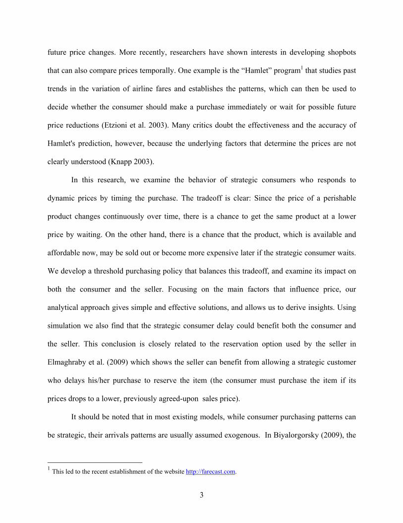
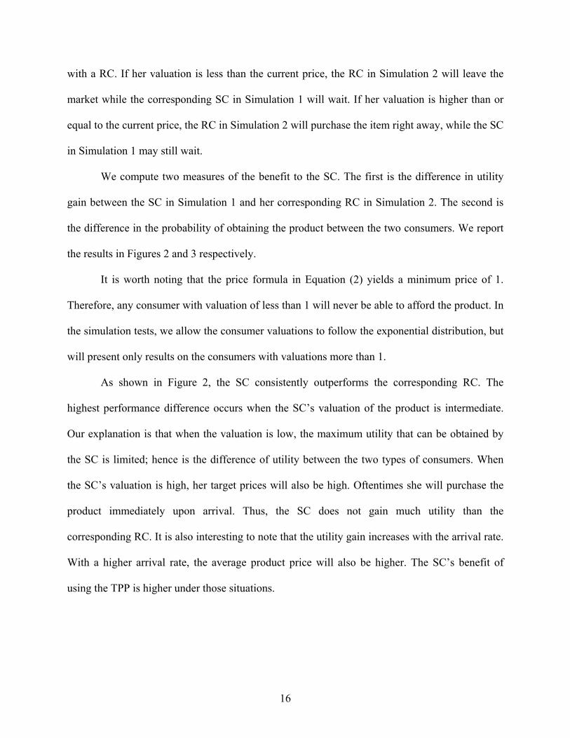
As shown in Figure 2, the SC consistently outperforms the corresponding RC. The

highest performance difference occurs when the SC’s valuation of the product is intermediate.

Our explanation is that when the valuation is low, the maximum utility that can be obtained by

the SC is limited; hence is the difference of utility between the two types of consumers. When

the SC’s valuation is high, her target prices will also be high. Oftentimes she will purchase the

product immediately upon arrival. Thus, the SC does not gain much utility than the

corresponding RC. It is also interesting to note that the utility gain increases with the arrival rate.

With a higher arrival rate, the average product price will also be higher. The SC’s benefit of

using the TPP is higher under those situations.

17

0.00

0.02

0.04

0.06

0.08

0.10

0.12

0.14

1.1 1.3 1.5 1.7 1.9 2.1 2.3 2.5

Valuation

Util

ity G

ain

a = 60a = 80a = 100a = 120a = 140

Figure 2. Average Utility Gain for SC

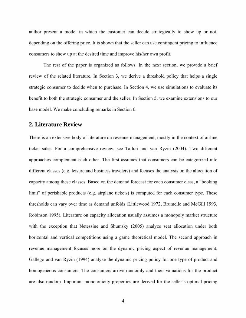
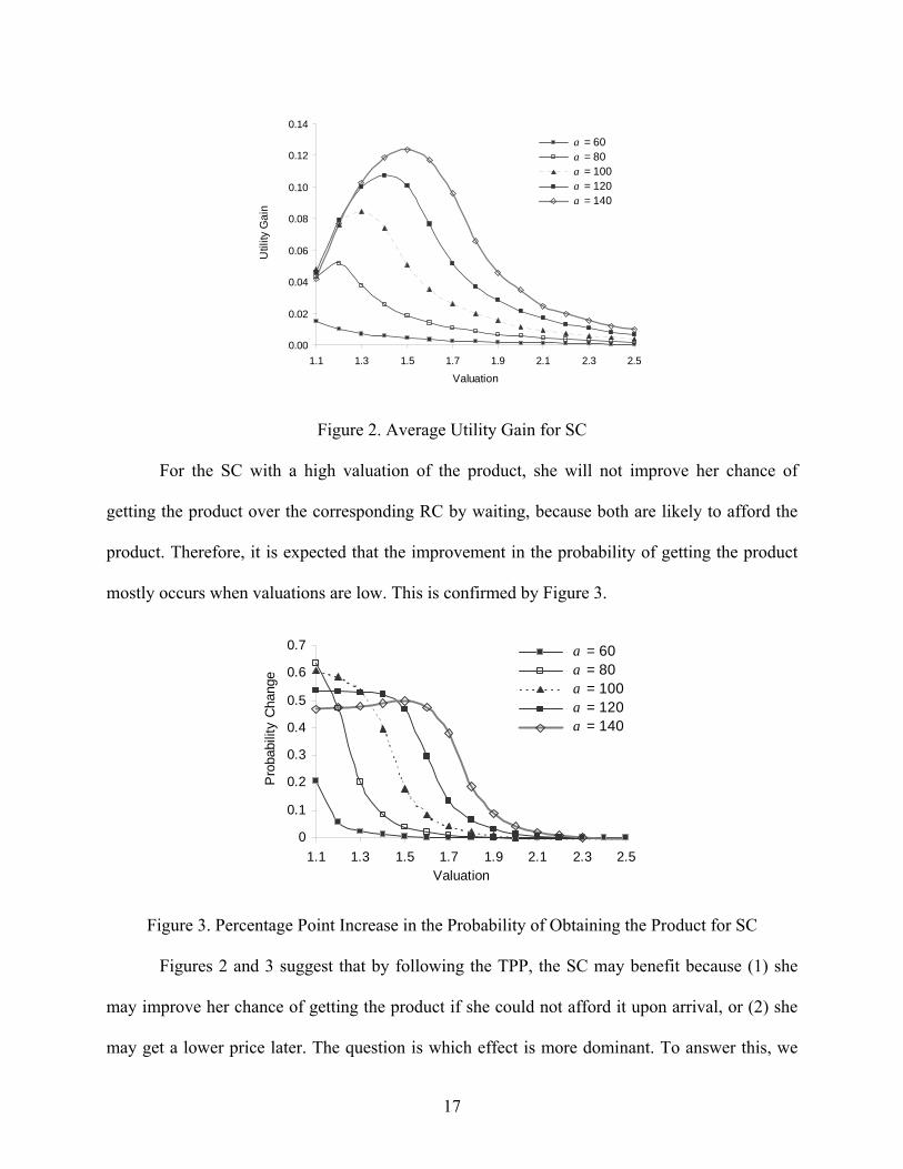
For the SC with a high valuation of the product, she will not improve her chance of

getting the product over the corresponding RC by waiting, because both are likely to afford the

product. Therefore, it is expected that the improvement in the probability of getting the product

mostly occurs when valuations are low. This is confirmed by Figure 3.

0

0.1

0.2

0.3

0.4

0.5

0.6

0.7

1.1 1.3 1.5 1.7 1.9 2.1 2.3 2.5Valuation

Pro

babi

lity

Cha

nge

a = 60a = 80a = 100a = 120a = 140

Figure 3. Percentage Point Increase in the Probability of Obtaining the Product for SC

Figures 2 and 3 suggest that by following the TPP, the SC may benefit because (1) she

may improve her chance of getting the product if she could not afford it upon arrival, or (2) she

may get a lower price later. The question is which effect is more dominant. To answer this, we

18

perform more detailed analysis. We categorize all the simulation outcomes into two cases. In

Case 1, the SC cannot afford the product upon arrival (i.e. v p< ). In Case 2, the SC can afford

the product upon arrival (i.e. v p≥ ). The corresponding RC, who has the same valuation as the

SC, will get a utility of 0 in Case 1. Thus, the SC will always be better off in Case 1. In Case 2,

there are three scenarios. First, the SC buys the product immediately. In this scenario, there is no

difference on the benefit. Second, the SC manages to purchase the product later. We believe that

on average she will be able to purchase at a lower price and, thus, is better off by waiting. Third,

the SC waits but does not get the product. Because the corresponding RC purchases the product,

the SC is worse off in this scenario.

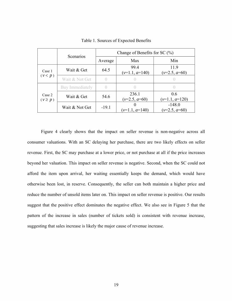
The simulation results show that the expected utility gain of SC is positive in both Cases

1 and 2, suggesting that on average the SC is always better off. Furthermore, we find that the

expected gain predominantly comes from Case 1 when the valuation is low and the arrival rate is

high. For example, about 99% of the benefit comes from Case 1 when v = 1.1 and a = 140, while

only 12% of the benefit comes from Case 1 when v = 2.5 and a=60. When the valuation is low

and the arrival rate is high, the price is less affordable, and the TPP allows the SC to have the

chance to purchase the product at a price lower than his valuation. When the price is more

affordable due to either a lower arrival rate or a higher consumer valuation, a higher percentage

of the expected gain comes from Case 2. Table 1 provides a summary.

4.2. Impact on the Seller

Since the use of the threshold purchase policy benefits the strategic consumer, one may expect

that the seller will be worse off if it continues to use the original dynamic pricing policy.

Revenue could decline because strategic consumers will delay their purchases and pay lower

prices. On the contrary, we find the sellers by and large do better with a strategic consumer.

19

Table 1. Sources of Expected Benefits

Change of Benefits for SC (%) Scenarios

Average Max Min

Wait & Get 64.5 99.4 (v=1.1, a=140)

11.9 (v=2.5, a=60) Case 1

( v p< ) Wait & Not Get 0 0 0

Buy Immediately 0 0 0

Wait & Get 54.6 236.1 (v=2.5, a=60)

0.6 (v=1.1, a=120)

Case 2 ( v p≥ )

Wait & Not Get -19.1 0 (v=1.1, a=140)

-148.0 (v=2.5, a=60)

Figure 4 clearly shows that the impact on seller revenue is non-negative across all

consumer valuations. With an SC delaying her purchase, there are two likely effects on seller

revenue. First, the SC may purchase at a lower price, or not purchase at all if the price increases

beyond her valuation. This impact on seller revenue is negative. Second, when the SC could not

afford the item upon arrival, her waiting essentially keeps the demand, which would have

otherwise been lost, in reserve. Consequently, the seller can both maintain a higher price and

reduce the number of unsold items later on. This impact on seller revenue is positive. Our results

suggest that the positive effect dominates the negative effect. We also see in Figure 5 that the

pattern of the increase in sales (number of tickets sold) is consistent with revenue increase,

suggesting that sales increase is likely the major cause of revenue increase.

20

0%

1%

2%

3%

1.1 1.3 1.5 1.7 1.9 2.1 2.3 2.5

Valuation

Rev

enue

Cha

nge

a=80a=100a=120

0%

1%

2%

3%

1.1 1.3 1.5 1.7 1.9 2.1 2.3 2.5

Valuation

Sale

s C

hang

e

a=80

a=100

a=120

Figure 4. Percentage of Revenue Change Figure 5. Percentage of Sales Change

Note in Figure 4 that the positive impact is most significant when consumer valuation is

low. Because consumer valuations are exponentially distributed, which favors low valuations,

the seller’s overall revenue increase should be significant. To see that, we conduct further

simulations by following a random SC, whose valuation follows the exponential distribution. We

find both the average seller revenue improvement and average sales improvement increase

increases in the arrival rate (Figure 6). Figures 2 and 6 together suggest that when the product is

“hot” (higher demand relative to supply), the use of the TPP results in higher benefits for both

the SC and the seller. To explain this, we note first that when the arrival rate is high, the price is

also high. Individual consumers are more likely to be priced out of the market when they arrive.

This may even happen to high-valuation consumers at the beginning of the sales horizon. With

the SC waiting, when price drops below the SC’s threshold price, the SC will purchase. Thus, the

SC provides a valuable demand cushion for the seller, especially when the arrival rate is high.

21

0

0.2

0.4

60 80 100 120 140

Arrival Rate

Rev

enue

0

0.2

0.4

60 80 100 120 140

Arrival Rate

Sale

s

Figure 6. Average Revenue and Sales Increase by Arrival Rate

Moreover, using standard deviation or CV to measure price volatility in the original GVR

model, we find that price volatility increases in the consumer arrival rate (Figure 7). Intuitively,

with a higher arrival rate, the seller will price products higher. However, if expected demand

does not materialize, the seller has to reduce the price more sharply. Therefore, the higher arrival

rate leads to higher price volatility.

0

0.04

0.08

0.12

0.16

0.2

40 60 80 100 120 140

Arrival Rate

Pric

e Vo

latil

ity

StandardDeviationCV

Figure 7. Price Volatility and Arrival Rate (n = 25)

It seems that the increase in both the SC’s utility and the seller’s revenue can be

explained by the increase in price volatility when the arrival rate is high. This is consistent with

the results in financial literature on the limit order trading discussed earlier. In general, when the

market is more volatile, individual market participants can benefit by being patient and waiting

22

to a threshold price. Essentially, it is a form of transferring demand over time. When demand is

stochastic, this practice will help improve the overall market performance as well. In financial

market, limit orders narrow the bid-ask spread (Chung et al. 1999) and reduce transaction costs.

In the market of perishable products studied in our research, the use of the TPP reduces wasteful

inventory and increases seller revenue.

5. Extensions

5.1. Multiple SCs and a Simplified Threshold Price Policy

Realizing that the strategic consumer’s waiting could increase sellers’ revenue, sellers may

develop a system to encourage consumer waiting. An interesting analogy, as mentioned early, is

that allowing limit orders in financial markets helps to improve the overall market performance

(Chung et al. 1999). There are many options to encourage consumers to stay around rather than

leave instantly when prices are too high. We consider a simple system that allows consumers to

indicate an intention of future purchase. For example, the seller can ask the consumer to create a

“wish list” of the product and the target price, as well as the email address where the consumer

can be informed when the price is reached.4

In this section, we numerically investigate the impact of such a system on the seller’s

revenue. In Section 4, we already study the impact of a single SC on the seller’s revenue; but a

target purchase system will be open to all the consumers and there likely will be more than one

SC. In our simulations, we let each consumer choose to use such a system with a certain

probability and systematically vary this probability. (We will continue to call these consumers

SC.) Prior studies have reported that, even after many years in existence, online searching

4 While this practice is quite common for online retailers such as Amazon.com, it is rare in the airline industry. Recently, however, Travelocity.com introduced a “FareWatcher” feature that allows users to be notified when the ticket price of a particular flight reaches a certain level or drops by a certain amount.

23

activities are still limited (Johnson et al. 2004, Montgomery et al. 2004). Therefore, we expect

the use of such a target purchase system to be limited as well. Consequently, we vary the

proportion of SCs from 2.5% to 15%.

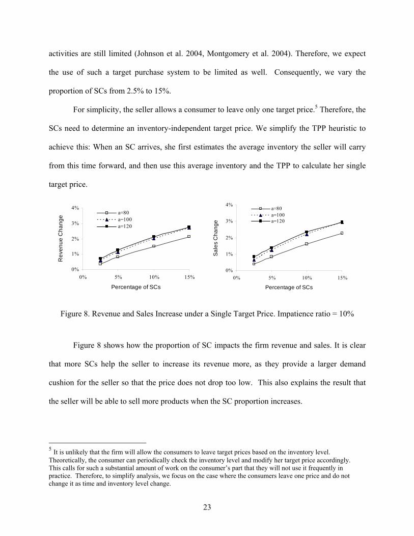
For simplicity, the seller allows a consumer to leave only one target price.5 Therefore, the

SCs need to determine an inventory-independent target price. We simplify the TPP heuristic to

achieve this: When an SC arrives, she first estimates the average inventory the seller will carry

from this time forward, and then use this average inventory and the TPP to calculate her single

target price.

0%

1%

2%

3%

4%

0% 5% 10% 15%

Percentage of SCs

Rev

enue

Cha

nge

a=80a=100a=120

0%

1%

2%

3%

4%

0% 5% 10% 15%

Percentage of SCs

Sal

es C

hang

ea=80a=100a=120

Figure 8. Revenue and Sales Increase under a Single Target Price. Impatience ratio = 10%

Figure 8 shows how the proportion of SC impacts the firm revenue and sales. It is clear

that more SCs help the seller to increase its revenue more, as they provide a larger demand

cushion for the seller so that the price does not drop too low. This also explains the result that

the seller will be able to sell more products when the SC proportion increases.

5 It is unlikely that the firm will allow the consumers to leave target prices based on the inventory level. Theoretically, the consumer can periodically check the inventory level and modify her target price accordingly. This calls for such a substantial amount of work on the consumer’s part that they will not use it frequently in practice. Therefore, to simplify analysis, we focus on the case where the consumers leave one price and do not change it as time and inventory level change.

24

It is an interesting research topic to examine how the seller should react when the portion

of SCs is more significant, but we do not pursue this further since it is beyond the scope of our

paper. Interested readers are referred to Su (2006).

5.2. Constraints on Strategic Consumer Waiting

Our model so far has assumed an infinitely patient SC who does not incur cost while waiting for

the target time/price. In this section, we exam two approaches that incorporate constraints on SC

waiting. First, we include waiting cost for the SC. Second, we consider impatient SCs.

In the first approach, we extend the base model by including a linear waiting cost. That

is, for every unit of time the SC waits, she incurs a cost of c , which can be a function of the SC’s

valuation v. For example, if the SC is waiting for an air ticket, then while waiting she has to

endure and manage the uncertainty imposed on her other activities during the trip (booking hotel,

rental car, tour etc.). It turns out that it is fairly straightforward to extend the base model to

include c . The following proposition parallels Proposition 3.

PROPOSITION 6. The kt s for the TTP are solutions to ( )

( , )

( , ) .,

p k ttv p k t c

k tλ

∂∂= + −

It is interesting to note that, in terms of choosing target times, the inclusion of c

effectively makes an SC with valuation v act like an SC with valuation v+c in the base model.

Using Proposition 4, we observe that the higher the waiting cost, the bigger the tks, and the

shorter the SC’s waiting time. Although intuitive, Proposition 6 provides a way to quantify the

effect of c.

Another way to incorporate the constraint on consumer waiting is to explicitly model

those consumers who wait but then leave the system before making a purchase; i.e. some SCs are

impatient. The difference between this approach and the waiting cost approach is akin to that

25

between abandonment and waiting cost in the queueing literature. We believe that abandonment

is a more realistic and robust way to model consumer waiting because the cost of waiting could

be difficult to quantify. Therefore, we focus on this approach in subsequent simulation studies.

In the simulations we allow a certain portion of SCs to be impatient. We call this portion

the impatience ratio. Those impatient SCs are randomly selected, and each has her own time-to-

abandonment which is uniformly distributed between their arrival time and the end of the sales

horizon. In addition to consumer impatience level, the impatience ratio can also reflect the level

of competition (e.g. how many airlines fly between the city pair on that date) and the level of

consumer loyalty (e.g. whether the consumer belongs to a loyalty program). In our simulations

we vary the impatience ratio from zero to fifteen percent.

0%

1%

2%

3%

0% 5% 10% 15%

SC Impatience Ratio

Rev

enue

Cha

nge

a=80 a=100 a=120

0%

1%

2%

3%

0% 5% 10% 15%

SC Impatience Ratio

Sale

s C

hang

e

a=80 a=100 a=120

Figure 9. Percentage of Impatient SCs and the Changes of Revenue and Sales

Figure 9 displays the impact of impatience ratio on seller revenue and sales. We set the

proportion of SCs of all consumers to 10% and let all the SCs follow a single target price

heuristic—the simplified TPP. Not surprisingly, as impatience ratio increases, both revenue and

sales increase decrease, but they remain positive.

26

Figures 9, together with Figure 8, also reveal that the revenue increase with SCs is higher

with a higher customer arrival rate. This again suggests that sellers with more price volatility

should benefit more by providing a target purchase option to their customers.

6. Conclusions and Future Research

In this research, we study the strategic response of consumers to dynamic prices of revenue

management. The SCs wait to purchase at specific target prices (TPP) or target times (TTP) that

depend on the consumers’ valuation of the product and the current inventory level. We present

an analytical model of the behavior of a single SC and derive the TPP and TTP. We also

conduct simulations to study the performance of the TTP/TPP. We show that consumers benefit

by following these policies. In particular we find that when the consumer valuation is low or the

arrival rate is high, most of the utility gains come from the improved probability of getting the

product by waiting (hence, the utility improves to non-zero from zero). When the consumer

valuation of the product is high, then most of the benefit comes from the lower price by waiting.

Overall, the benefit is the greatest for low-valuation consumers (low v) and hot products (high a).

We also show that the firm also benefits from having SCs who follow the TTP/TPP. This

result first seems to be counter-intuitive until one realizes that this is not a zero-sum game. The

firm may benefit because, while RCs will leave the market if they cannot afford the product upon

arrival, SCs are kept in the waiting pool, especially early in the sales period when the product

price is usually higher. This waiting of SCs provides a cushion to price volatility and prevents

the price from falling too low. It also serves as an additional demand that helps to reduce wasted

inventory at the end. This benefit is somewhat similar to the benefits of limit orders in stock

trading which provide liquidity to the market (Chung et al. 1999, Forcault 1999).

27

When high-valuation SCs wait and get a lower price, this will negatively affect the firm’s

revenue. But our results show that, in general, the potential revenue loss from the delay of

purchase is limited. High-valuation consumers, as it turns out, have higher target prices, and are

very likely to purchase immediately upon arrival. Keeping low-valuation consumers in the

waiting pool helps to reduce wasted inventory and prevent firms from deep price discounts

toward the end. This could be especially beneficial to industries with a fixed cost for the

products, e.g. airline tickets and hotel rooms, where the revenue loss of each wasted inventory is

large.

This discovery of benefits to the firm is important as it encourages companies to develop

systems that can allow consumers to place a “limit order” for the products or services. Actual

implementation can be flexible. Consumers can choose to be notified of price changes through

emails. A promising direction for future research is to model the impact of such practices on

firm’s revenue analytically and quantify the tradeoffs between the higher sales and the lower

prices paid by some consumers.

The analytical results in this paper are based on the modeling of a single SC.

Nevertheless, simulation results show that with multiple SCs, the benefits to each individual SC

(the utility gain and the probability of obtaining the product) remains quite stable, while the

benefit to the firm (higher revenue) increases with the proportion of SCs. This result holds for

small proportions of SCs (2.5%–15%). As the proportion increases, the benefit to the firm may

plateau; but more importantly SCs will be aware of the existence and impact of other SCs. Their

purchasing behavior will adjust accordingly. Similarly, the seller may also need to adopt a

different pricing formula when the proportion is high. A game theoretical framework is

28

necessary to study these issues. It is beyond the scope of this paper, but is certainly an

interesting direction for future research.

Reference

Anderson, C.K. and J.G. Wilson. 2003. Wait or buy? The strategic consumer: Pricing and profit

implications. Journal of the Operational Research Society 54 (3), 299-306.

Aviv, Y. and A. Pazgal. 2003. Optimal pricing of seasonal products in the presence of forward-

looking consumers. Working Paper, Olin School of Business, Washington University.

Available at: http://www.olin.wustl.edu/faculty/aviv/.

Belobaba, P. 1989. Application of a probabilistic decision model to airline seat inventory control.

Operations Research 37, 183-197.

Besanko, D. and W. Winston. 1990. Optimal price skimming by a monopolist facing rational

consumers. Management Science 36(5), 555-567.

Bitran, G. and R. Caldentey. 2003. An overview of pricing models for revenue management.

Manufacturing & Service Operations Management 5 (3), 203 –229.

Biyalorgorsky, E. 2009. Shaping Consumer Demand through the Use of Contingent Pricing, in

Operations Management Models with Consumer-Driven Demand, edited by Serguei

Netessine and Christopher S. Tang, Springer.

Brumelle, S.L. and J.I. McGill. 1993. Airline seat allocation with multiple nested classes.

Operations Research 41 127-137.

Choi, S. and S.E. Kimes. 2002. Electronic distribution channel's effect on hotel revenue

management. Cornell Hotel and Restaurant Administration Quarterly 43 (3), 23-31.

29

Chung, K., B. Van Ness, R. Van Ness. 1999. Limit orders and the bid-ask spread. Journal of

Financial Economics 53, 255-287.

Elmaghraby, W., A. Gulcu, and P. Keskinocak. 2005. Optimal markdown mechanisms in the

presence of rational consumers with multi-unit demands. Working paper, Georgia

Institute of Technology. Available at:

http://www.smith.umd.edu/faculty/welmaghraby/pdf/markdown.pdf.

Elmaghraby, W., S. Lippman, C.S. Tang, and R. Yin 2009. Will More Purchasing Options

Benefit Customers? Forthcoming, Production and Operations Management.

Etzioni, O., C. Knoblock, R. Tuchinda, and A. Yates, 2003. To buy or not to buy: Mining airfare

data to minimize ticket purchase price. SIGKDD ’03, August 24-27, 2003. Washington,

DC, USA.

Foucault, T. 1999. Order flow composition and trading costs in a dynamic limit order market.

Journal of Financial Markets 2, 99-134.

Gallego, G. and G. van Ryzin. 1994. Optimal dynamic pricing of inventories with stochastic

demand over finite horizon. Management Science 40, 999-1020.

Harris, L. and J. Hasbrouck. 1996. Market vs. limit orders: the SuperDOT evidence on order

submission strategy. Journal of Financial and Quantitative Analysis 31, 213-231.

Ho, T., C.S. Tang, and D.R. Bell. 1998. Rational shopping behavior and the option value of

variable pricing. Management Science 44, 145-160.

Johnson, E., W. Moe, P. Fader, S. Bellman, and G. Lohse. 2004. On the depth and dynamics of

online search behavior. Management Science 50 (3), 299-308.

Kimes, S.E. 1989. Yield management: a tool for capacity-constrained service firm. Journal of

Operations Management 8, 348-363.

30

Kincaid, W. M., D. A. Darling. 1963. An inventory pricing problem. Journal of

Mathematical Analysis and Applications 7 (2), 183–208.

Knapp, L. April 9, 2003. Algorithms key to cheap air fare. Wired News.

Liddle, A. 2003. Using web for discounting clicks with digital diners. Nation's Restaurant News

37 (20), 172.

Littlewood, K. 1972. Forecasting and control of passengers. 12th AGIFORS Symposium

Proceedings. Nathanya, Israel 95–128.

Liu, Q. and G. van Ryzin. 2005. Strategic capacity rationing to induce early purchases.

Manufacturing & Service Operations Management 8(1), 110-115.

McGill, J. and G. van Ryzin. 1999. Revenue Management: Research Overview and Prospects.

Transportation Science 33, 233-256.

Montgomery, A., K. Hosanagar, R. Krishnan, and K. Clay. 2004. Designing a better shopbot.

Management Science 50 (2), 189-206.

Netessine, S. and R.A. Shumsky. 2005. Revenue management games: Horizontal and Vertical

Competition. Management Science 51 (5), 813-831.

Robinson, L.W. 1995. Optimal and approximate control policies for airline booking with

sequential nonmonotonic fare classes. Operations Research 43 252-263.

Su, X. 2006. Inter-temporal pricing with strategic customer behavior. Working Paper, University

of California, Berkeley. Available at: http://faculty.haas.berkeley.edu/xuanming/.

Talluri, K., and G. van Ryzin. 2004. The theory and practice of revenue management. Kluwer

Academic Publishers.

Zhao, W., and Y. Zheng. 2000. Optimal dynamic pricing for perishable assets with

nonhomogeneous demand. Management Science 46, 375-388.

31

32

Appendix

PROOF OF PROPOSITION 1.

Because the pricing curves ( , )p k t are strictly increasing in t for the fixed k, it is easy to show

that there exists a one-to-one relationship between tk and ( , )k kp p k t= such that t > tk ⇔ p > pk,

and t < tk ⇔ p < pk. Thus, there is a one-to-one correspondence between the TPP and the TTP.■

PROOF OF PROPOSITION 2.

Suppose that the SC arrives in the state (k,t) and sees the price ( , )p k t . We denote ( , , )iq k t tΔ

the probability of i consumers arriving during [ , ]t t t− Δ who can afford ( , )p k t . It is easy to

see 00lim ( , , ) 1

tq k t t

Δ →Δ = , ( )1

0

( , , )lim ( , )t

q k t t p k tt

λΔ →

Δ=

Δ, and

2( , , ) ( )i

iq k t t o t

≥

Δ = Δ∑ . If the SC

purchases the product at t, the realized utility is ( , )v p k t− . If the SC waits and purchases after

tΔ , the expected utility is

{ } [ ]1 0( , , ) max 0, ( 1, ) ( , , ) ( , ) ( )q k t t v p k t t q k t t v p k t t o tΔ − − − Δ + Δ − − Δ + Δ . (A.1)

At the threshold tk, the SC is indifferent between purchasing and waiting a little bit. By equating

these two utilities and letting tΔ go to 0, we obtain

[ ]

{ } [ ]

1 0

0

100

1 ( , , ) ( , , )lim ( , )

( , ) ( , )( , , ) ( )lim ( , ) min ( 1, ), ( , , ) .

t

t

q k t t q k t t v p k tt

p k t p k t tq k t t o tp k t p k t t v q k t tt t t

Δ →

Δ →

− Δ − Δ⎡ ⎤ −⎢ ⎥Δ⎣ ⎦⎧ ⎫− −ΔΔ Δ

= − − −Δ + Δ +⎡ ⎤⎨ ⎬⎣ ⎦Δ Δ Δ⎩ ⎭

This

amounts to ( ) { }0 ( , ) ( , ) min ( 1, ), ( , )p k t p k t p k t v p k tt

λ ∂= − − +⎡ ⎤⎣ ⎦ ∂

. Therefore, the time threshold

tk satisfies: { } ( )

( , )min ( 1, ), ( , ) .

( , )

p k ttp k t v p k tp k tλ

∂∂− = + ■

33

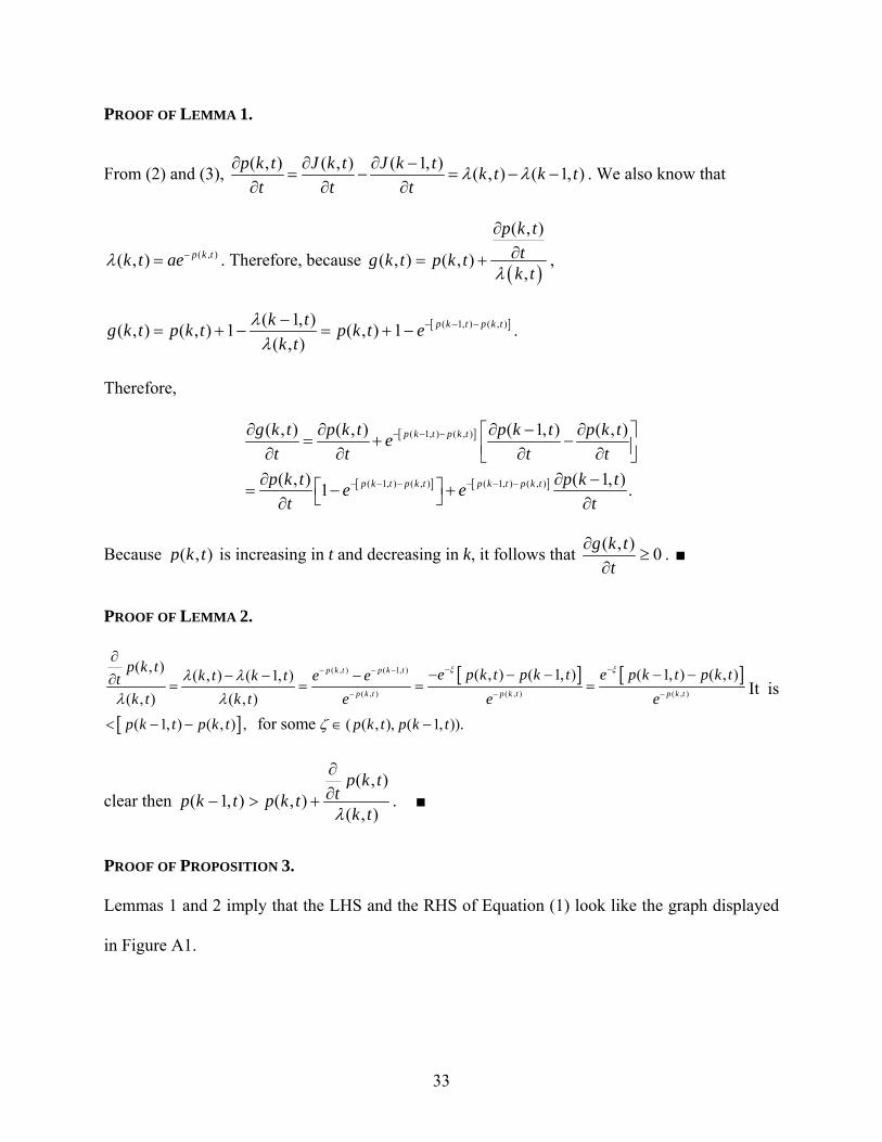
PROOF OF LEMMA 1.

From (2) and (3), ( , ) ( , ) ( 1, ) ( , ) ( 1, )p k t J k t J k t k t k tt t t

λ λ∂ ∂ ∂ −= − = − −

∂ ∂ ∂. We also know that

( , )( , ) p k tk t aeλ −= . Therefore, because ( )

( , )

( , ) ( , ),

p k ttg k t p k t

k tλ

∂∂= + ,

[ ]( 1, ) ( , )( 1, )( , ) ( , ) 1 ( , ) 1( , )

p k t p k tk tg k t p k t p k t ek t

λλ

− − −−= + − = + − .

Therefore,

[ ]

[ ] [ ]

( 1, ) ( , )

( 1, ) ( , ) ( 1, ) ( , )

( , ) ( , ) ( 1, ) ( , )

( , ) ( 1, )1 .

p k t p k t

p k t p k t p k t p k t

g k t p k t p k t p k tet t t t

p k t p k te et t

− − −

− − − − − −

∂ ∂ ∂ − ∂⎡ ⎤= + −⎢ ⎥∂ ∂ ∂ ∂⎣ ⎦∂ ∂ −⎡ ⎤= − +⎣ ⎦∂ ∂

Because ( , )p k t is increasing in t and decreasing in k, it follows that ( , ) 0g k tt

∂≥

∂. ■

PROOF OF LEMMA 2.

[ ] [ ]

[ ]

( , ) ( 1, )

( , ) ( , ) ( , )

( , ) ( , ) ( 1, ) ( 1, ) ( , )( , ) ( 1, )( , ) ( , )

( 1, ) ( , ) , ( ( , ), ( 1, )) for some .

p k t p k t

p k t p k t p k t

p k t e p k t p k t e p k t p k tk t k t e etk t k t e e e

p k t p k t p k t p k t

ξ ξλ λλ λ

ζ

− −− − −

− − −

∂− − − − −− − −∂ = = = =

< − − ∈ −

It is

clear then ( , )

( 1, ) ( , )( , )

p k ttp k t p k t

k tλ

∂∂− > + . ■

PROOF OF PROPOSITION 3.

Lemmas 1 and 2 imply that the LHS and the RHS of Equation (1) look like the graph displayed

in Figure A1.

34

(i) From Figure A1, it is clear that, because ( 1, )p k t− is always greater than the RHS, kt is the

intersection of v and the RHS. In effect, Equation (1) can be simplified to

( )

( , )( , ) .

( , )

p k ttv p k tp k tλ

∂∂= + (A.2)

(ii) Next, we prove that the two curves will intersect if and only if 1v ≥ . Since the RHS is

increasing in t, its minimum is achieved at 0t = , which is 1. So clearly v needs to be at least one.

On the other hand, when t goes to 0, the RHS goes to 1; and when t goes to ∞, the value goes to

∞. Because the RHS is continuous, we conclude that for any v ≥ 1, there exists a tk such that the

equality holds. The uniqueness follows easily from the monotonicity of the RHS (Lemma 1). ■

PROOF OF PROPOSITION 4.

(i) follows immediately from Figure A1. For (ii), we note that

[ ]

[ ] [ ]

( 1, ) ( , )

( 1, ) ( , ) ( 1, ) ( , )

( , ) ( , ) ( 1, ) ( , )

( , ) ( 1, )1 .

p k t p k t

p k t p k t p k t p k t

g k t p k t p k t p k tea a a a

p k t p k te ea a

− − −

− − − − − −

∂ ∂ ∂ − ∂⎡ ⎤= + −⎢ ⎥∂ ∂ ∂ ∂⎣ ⎦∂ ∂ −⎡ ⎤= − +⎣ ⎦∂ ∂

Figure A1. Solution to the Threshold Policy.

0 0.2 0.4 0.6 0.8 1

t

LHS RHS

v

tk

35

Because ( , )p k t is increasing in a, it follows that ( , )g k t is also increasing in a. Clearly from

Figure A1, as the RHS increases and v stays the same, the intersection point, kt , decreases. ■

PROOF OF PROPOSITION 5.

First of all, note the following:

[ ].1),(

),1(1

),(),1(),(

),(

),(

),(

),(),1( kk tkptkp

k

k

k

kk

k

k

kk

evtk

tkv

tktktkv

tkt

tkp

vtkpp

−−−+−=−

+−=

−−−=∂

∂

−==

λλ

λλλ

λ (A.3)

Because ⎟⎟⎠

⎞⎜⎜⎝

⎛= ∑

=

k

i

i

ieattkJ

0 !)/(log),( and 1),1(),(),( +−−= tkJtkJtkp , both ),( tkJ and ),( tkp

depend on a only through the product at. So if we let atx = then both ),( tkJ and ),( tkp

become functions of only x (i.e. they are free of a). Therefore, we can simply solve (A.2) to

obtain kk atx = and plug them into (A.3) to compute kp . The kp s thus computed are all free of

a. ■

PROOF OF PROPOSITION 6.

This proof is very similar to that of Proposition 2. If the SC purchases the product at t, the

realized utility is ( , )v p k t− . If the SC waits and purchases after tΔ , the expected utility is

{ } [ ]1 0( , , ) max 0, ( 1, ) ( , , ) ( , ) ( )q k t t v p k t t q k t t v p k t t o tc tΔ − − − Δ + Δ − − Δ + Δ− Δ . (A.4)

At the threshold tk, the SC is indifferent between purchasing and waiting a little bit. By equating

these two utilities and letting tΔ go to 0, we obtain

[ ]

{ } [ ]

1 0

0

100

1 ( , , ) ( , , )lim ( , )

( , ) ( , )( , , ) ( )lim ( , ) min ( 1, ), ( , , ) .

t

t

q k t t q k t t v p k tt

p k t p k t tq k t t o tp k t p k t t v q k t t ct t t

Δ →

Δ →

− Δ − Δ⎡ ⎤ −⎢ ⎥Δ⎣ ⎦⎧ ⎫− −ΔΔ Δ

= − − −Δ + Δ − +⎡ ⎤⎨ ⎬⎣ ⎦Δ Δ Δ⎩ ⎭

36

This amounts to ( ) { }0 ( , ) ( , ) min ( 1, ), ( , )p k t p k t p k t v p k t ct

λ ∂= − − + −⎡ ⎤⎣ ⎦ ∂

. Therefore, the time

threshold tk satisfies:

{ } ( )

( , )min ( 1, ), ( , ) .

( , )

p k ttp k t v p k t cp k tλ

∂∂− = + − (A.5)

If kt t≥ , the strategic consumer will purchase right away; and if tk < t, the strategic

consumer will wait and the target purchase time is kt . Also, similar to Lemmas 1 and 2 (the

proofs are hence omitted), we can show that

1) ( )

( , )

( , ),

p k ttp k t c

k tλ

∂∂+ − is increasing in t, and

2) ( )

( , )

( 1, ) ( , ),

p k ttp k t p k t c

k tλ

∂∂− > + − .

The second result above allows us to simplify (A.3) to ( )

( , )

( , ),

p k ttv p k t c

k tλ

∂∂= + − , which completes

the proof. We note, from Figure A1, that a positive c will increase the target time tks, which

means the SC is willing to wait less when there is a cost. While this is intuitive, Propositions 3

and 6 show a way to quantify the difference. ■