Embed Size (px)
Citation preview
Strategic BiopharmaceuticalProduction Planning for Batch
and Perfusion Processes
A thesis submitted to UCL
for the degree of
Engineering Doctorate
by
Cyrus Carlos Siganporia
The Advanced Centre for Biochemical EngineeringDepartment of Biochemical Engineering
UCLTorrington PlaceLondon WC1E 7JE
July, 2016

2

Declaration
I, Cyrus Siganporia, confirm that the work presented in this thesis is my own.
Where information has been derived from other sources, I confirm that this has
been indicated in the thesis.
3

4

Abstract
Capacity planning for multiple biopharmaceutical therapeutics across a large net-
work of manufacturing facilities, including contract manufacturers, is a complex
task. Production planning is further complicated by portfolios of products requir-
ing different modes of manufacture: batch and continuous. Capacity planning
decisions each have their own costs and risks which must be carefully considered
when determining manufacturing schedules. Hence, this work describes a frame-
work which can assimilate various input data and provide intelligent capacity
planning solutions.
First of all, a mathematical model was created with the objective of min-
imising total cost. Various challenges surrounding the biomanufacturing of both
perfusion and fed-batch products were solved. Sequence-dependent changeover
times and full decoupling between upstream and downstream production suites
were incorporated into the mixed integer linear program, which was used on an
industrial case study to determine optimal manufacturing schedules and capital
expenditure requirements. The effect of varying demands and fermentation titres
was investigated via scenario analysis. To improve computational performance
of the model, a rolling time horizon was introduced, and was shown to not only
improve performance but also solution quality.
The performance of the model was then improved via appropriate reformu-
lations which consider the state task network (STN) topology of the problem
domain. Two industrial case studies were used to demonstrate the merits of
using the new formulation, and results showed that the STN improved perfor-
mance in all test cases, and even performed better than the rolling time horizon
5

approach from the previous model in one test case. Various strategic options
regarding capacity expansion were analysed, in addition to an illustration of how
the framework could be used to de-bottleneck existing capacity issues.
Finally, a multi-objective component is added to the model, enabling the con-
sideration of strategic multi-criteria decision making. The ε-constraint method
was shown to be the superior multi-objective technique, and was used to demon-
strate how uncertain input parameters could affect the different objectives and
capacity plans in question.
6

Acknowledgements
I would like to thank my academic supervisor, Prof. Suzanne Farid, for her
continual support, trust and insightful guidance throughout the course of my
project. I would also like to show my appreciation to Prof. Lazaros Papageorgiou,
who has provided fruitful discussions and directions surrounding my thesis. I
wish to extend my gratitude to Bayer Technology Services, in particular Soumitra
Ghosh, Christian Ramsch, Andreas Schluck, Brijesh Tanjore Vasudeva Rao, Todd
Roman, Scott Probst, and Thomas Daszkowski. Their time, supervision and
industrial knowledge was immensely useful in developing this work.
I wish to thank the UK Engineering and Physical Sciences Research Coun-
cil (EPSRC) Centre for Innovative Manufacturing in Emergent Macromolecular
Therapies, hosted by UCL with Imperial College London and a consortium of
industrial and government users. Financial support from the EPSRC and Bayer
Technology Services is gratefully acknowledged.
I wish to extend my thanks to friends who have helped along the way, includ-
ing Songsong Liu and Richard Allmendinger. Finally, I would like to thank my
family for their patience and kindness throughout my doctorate degree.
7

8

Contents
1 Literature Review 13
1.1 Biopharmaceutical Drug Development and Manufacturing . . . . . 14
1.2 Problems Facing the Biopharmaceutical Industry . . . . . . . . . . 16
1.3 Current Industrial Practice . . . . . . . . . . . . . . . . . . . . . . 20
1.4 Mathematical Programming . . . . . . . . . . . . . . . . . . . . . . 22
1.4.1 Linear programming . . . . . . . . . . . . . . . . . . . . . . 22
1.4.2 Techniques . . . . . . . . . . . . . . . . . . . . . . . . . . . 25
1.4.3 Multi-objective methods . . . . . . . . . . . . . . . . . . . . 29
1.5 Alternative Heuristic Search Methods . . . . . . . . . . . . . . . . 31
1.5.1 Simulated annealing . . . . . . . . . . . . . . . . . . . . . . 31
1.5.2 Genetic algorithms . . . . . . . . . . . . . . . . . . . . . . . 33
1.5.3 Swarm intelligence . . . . . . . . . . . . . . . . . . . . . . . 35
1.6 Justification of Mathematical Programming Approach . . . . . . . 37
1.7 Aims and Organisation of Thesis . . . . . . . . . . . . . . . . . . . 37
2 Requirements and Analysis 41
2.1 Detailed Problem Statement . . . . . . . . . . . . . . . . . . . . . . 41
2.2 Computational Complexity . . . . . . . . . . . . . . . . . . . . . . 45
2.3 Framework Structure . . . . . . . . . . . . . . . . . . . . . . . . . . 46
2.4 Model Requirements . . . . . . . . . . . . . . . . . . . . . . . . . . 47
2.5 Summary . . . . . . . . . . . . . . . . . . . . . . . . . . . . . . . . 49
3 Capacity planning for batch and perfusion bioprocesses across
multiple biopharmaceutical facilities 51
9

CONTENTS
3.1 Introduction . . . . . . . . . . . . . . . . . . . . . . . . . . . . . . . 51
3.2 Problem Definition . . . . . . . . . . . . . . . . . . . . . . . . . . . 53
3.2.1 Facility features . . . . . . . . . . . . . . . . . . . . . . . . . 53
3.2.2 Fed-batch versus perfusion culture processes . . . . . . . . . 54
3.2.3 Key performance indicators . . . . . . . . . . . . . . . . . . 56
3.3 Mathematical formulation and solution procedure . . . . . . . . . . 57
3.3.1 Technical and commercial constraints . . . . . . . . . . . . 57
3.3.2 Objective function . . . . . . . . . . . . . . . . . . . . . . . 66
3.3.3 Optimisation Strategies . . . . . . . . . . . . . . . . . . . . 67
3.4 Illustrative Example . . . . . . . . . . . . . . . . . . . . . . . . . . 68
3.4.1 Input Data . . . . . . . . . . . . . . . . . . . . . . . . . . . 68
3.4.2 Computational Results . . . . . . . . . . . . . . . . . . . . . 72
3.4.3 Computational Statistics . . . . . . . . . . . . . . . . . . . 78
3.5 Summary . . . . . . . . . . . . . . . . . . . . . . . . . . . . . . . . 80
3.6 Nomenclature . . . . . . . . . . . . . . . . . . . . . . . . . . . . . . 82
4 Biopharmaceutical Capacity Planning using a State Task Net-
work Topology 85
4.1 Introduction . . . . . . . . . . . . . . . . . . . . . . . . . . . . . . . 85
4.2 Problem Definition . . . . . . . . . . . . . . . . . . . . . . . . . . . 87
4.2.1 State-Task Network . . . . . . . . . . . . . . . . . . . . . . 87
4.2.2 Perfusion ramp-up times . . . . . . . . . . . . . . . . . . . . 88
4.2.3 Retrofitting considerations . . . . . . . . . . . . . . . . . . . 89
4.2.4 Contract manufacturing . . . . . . . . . . . . . . . . . . . . 89
4.2.5 Decentralised production . . . . . . . . . . . . . . . . . . . 90
4.2.6 Multi-purpose facilities . . . . . . . . . . . . . . . . . . . . . 90
4.3 Mathematical Formulation . . . . . . . . . . . . . . . . . . . . . . . 91
4.3.1 Technical and commercial constraints . . . . . . . . . . . . 91
4.3.2 Objective function . . . . . . . . . . . . . . . . . . . . . . . 102
4.4 Illustrative Example . . . . . . . . . . . . . . . . . . . . . . . . . . 104
4.5 Results . . . . . . . . . . . . . . . . . . . . . . . . . . . . . . . . . . 107
10

CONTENTS
4.5.1 Model size . . . . . . . . . . . . . . . . . . . . . . . . . . . . 108
4.5.2 Performance comparison . . . . . . . . . . . . . . . . . . . . 109
4.5.3 Effect of new features on production planning . . . . . . . . 116
4.5.4 Decentralised manufacturing . . . . . . . . . . . . . . . . . 117
4.5.5 Retrofitting a multi-purpose facility . . . . . . . . . . . . . 120
4.5.6 De-bottlenecking production plans . . . . . . . . . . . . . . 122
4.6 Summary . . . . . . . . . . . . . . . . . . . . . . . . . . . . . . . . 124
4.7 Nomenclature . . . . . . . . . . . . . . . . . . . . . . . . . . . . . . 126
5 Multi-Criteria Strategic Planning for Biopharmaceutical Pro-
duction 129
5.1 Introduction . . . . . . . . . . . . . . . . . . . . . . . . . . . . . . . 129
5.2 Problem Definition . . . . . . . . . . . . . . . . . . . . . . . . . . . 130
5.2.1 Multi-objective criteria . . . . . . . . . . . . . . . . . . . . 130
5.3 Mathematical Formulation . . . . . . . . . . . . . . . . . . . . . . . 131
5.3.1 Goal programming . . . . . . . . . . . . . . . . . . . . . . . 131
5.3.2 ε-constraint method . . . . . . . . . . . . . . . . . . . . . . 133
5.4 Illustrative Example . . . . . . . . . . . . . . . . . . . . . . . . . . 136
5.5 Results . . . . . . . . . . . . . . . . . . . . . . . . . . . . . . . . . . 140
5.5.1 Comparing multi-objective methods . . . . . . . . . . . . . 140
5.5.2 Effect of variability on multi-objective criteria . . . . . . . . 143
5.6 Summary . . . . . . . . . . . . . . . . . . . . . . . . . . . . . . . . 148
5.7 Nomenclature . . . . . . . . . . . . . . . . . . . . . . . . . . . . . . 149
6 Conclusions and Future Work 151
6.1 Introduction . . . . . . . . . . . . . . . . . . . . . . . . . . . . . . . 151
6.2 Contributions of this thesis . . . . . . . . . . . . . . . . . . . . . . 152
6.2.1 Capacity planning for batch and perfusion bioprocesses across
multiple biopharmaceutical facilities . . . . . . . . . . . . . 153
6.2.2 Biopharmaceutical Capacity Planning using a State Task
Network Topology . . . . . . . . . . . . . . . . . . . . . . . 153
11
CONTENTS
6.2.3 Multi-Criteria Strategic Planning for Biopharmaceutical Pro-
duction . . . . . . . . . . . . . . . . . . . . . . . . . . . . . 154
6.3 Recommendations for Future Work . . . . . . . . . . . . . . . . . . 154
6.3.1 Problem features . . . . . . . . . . . . . . . . . . . . . . . . 155
6.3.2 Uncertainty . . . . . . . . . . . . . . . . . . . . . . . . . . . 157
6.3.3 Alternative search heuristics . . . . . . . . . . . . . . . . . . 158
References 159
Appendix A Genetic algorithm optimisation procedure 173
Appendix B Papers by the author 183
12

Chapter 1
Literature Review
The biopharmaceutical industry has grown enormously since the first drug was
released to the market in 1982. In the year 2000, there were 84 biopharmaceuticals
approved globally, and by 2014 that number had grown to almost 250 (Walsh,
2014). However, this number may be closer to 170, since some of the therapeutics
are very similar to each other biologically. This rapid growth is largely down
to advances in molecular biology technology, providing improved platforms for
the discovery and manufacture of monoclonal antibodies, protein hormones and
genetically engineered vaccines (three major biopharmaceuticals). The success of
these drugs can be measured by the profitability and growth of the companies
manufacturing them. In 2014 alone, revenue for biopharmaceutical companies
within the US, Europe, Canada and Australia increased by 24% (Ernst & Young,
2015). However, these biopharmaceutical drugs take approximately 8 years to
go from initial development to reaching the market, placing huge pressures on
the companies to reduce development and manufacturing costs (Foo et al., 2001).
This, along with the inherent risks associated with biopharmaceutical sector,
provides the reasoning behind the development of a decision support tool to help
the industry perform more efficiently under uncertain conditions.
This chapter will discuss the development process of new drugs, and the
pressures facing the biopharmaceutical industry. It will also describe some work
that has already been carried out on capacity planning, and explain some of the
techniques used in optimisation.
13
CHAPTER 1. LITERATURE REVIEW
1.1 Biopharmaceutical Drug Development and Man-
ufacturing
In order to get a drug to the market, it must first undergo preclinical and clinical
trials, and then if successful, a New Drug Application (NDA) can be applied
for and the drug then sold to the market. However, many drug candidates will
be unsuccessful, and thus biopharmaceutical companies must develop many drug
candidates simultaneously so that hopefully at least one will succeed. In general,
only 1 in every 5,000 to 10,000 molecules that enter the drug discovery stage will
successfully reach the market (Lipsky and Sharp, 2001), and on average it takes
8-12 years and has been estimated to cost between $1 - 1.8 billion (Adams and
Brantner, 2010; Paul et al., 2010). The drug discovery stage involves computa-
tional chemistry, which is followed by 2-4 years of preclinical studies on animals.
If successful, an investigational new drug (IND) application can be opened with
the Food and Drug Administration (FDA), and then clinical trials on humans
can begin. Phase I, II, and III take approximately one, two, and three years
respectively to complete, and finally the manufacturer files for an NDA with the
FDA for approval. Sometimes the FDA requires further studies to be undertaken
before approval can be granted. Even after granting approval they can ask the
manufacturer to continue post-marketing studies, especially for drugs which are
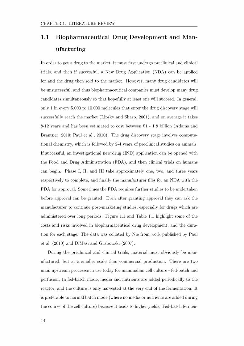
administered over long periods. Figure 1.1 and Table 1.1 highlight some of the
costs and risks involved in biopharmaceutical drug development, and the dura-
tion for each stage. The data was collated by Nie from work published by Paul
et al. (2010) and DiMasi and Grabowski (2007).
During the preclinical and clinical trials, material must obviously be man-
ufactured, but at a smaller scale than commercial production. There are two
main upstream processes in use today for mammalian cell culture - fed-batch and
perfusion. In fed-batch mode, media and nutrients are added periodically to the
reactor, and the culture is only harvested at the very end of the fermentation. It
is preferable to normal batch mode (where no media or nutrients are added during
the course of the cell culture) because it leads to higher yields. Fed-batch fermen-
14
CHAPTER 1. LITERATURE REVIEW
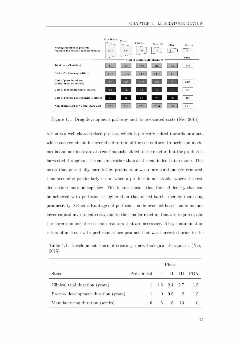
Figure 1.1: Drug development pathway and its associated costs (Nie, 2015)
tation is a well characterised process, which is perfectly suited towards products
which can remain stable over the duration of the cell culture. In perfusion mode,
media and nutrients are also continuously added to the reactor, but the product is
harvested throughout the culture, rather than at the end in fed-batch mode. This
mean that potentially harmful by-products or waste are continuously removed,
thus becoming particularly useful when a product is not stable, where the resi-
dence time must be kept low. This in turn means that the cell density that can
be achieved with perfusion is higher than that of fed-batch, thereby increasing
productivity. Other advantages of perfusion mode over fed-batch mode include
lower capital investment costs, due to the smaller reactors that are required, and
the fewer number of seed train reactors that are necessary. Also, contamination
is less of an issue with perfusion, since product that was harvested prior to the
Table 1.1: Development times of creating a new biological therapeutic (Nie,2015)
Phase
Stage Pre-clinical I II III FDA
Clinical trial duration (years) 1 1.6 2.4 2.7 1.5
Process development duration (years) 1 0 0.5 2 1.5
Manufacturing duration (weeks) 6 5 5 13 0
15
CHAPTER 1. LITERATURE REVIEW
contamination is still viable (checks are made with every harvest, which is often
daily), whereas with fed-batch mode the entire batch would have to be discarded.
These advantages of perfusion mode over fed-batch mode can sometimes lead to
manufacturers choosing perfusion during clinical trial phases (where production
quantities are low and thus do not warrant the higher investment costs for batch
systems), but then move to fed-batch mode for production quantity (Meuwly
et al., 2006). The reason for this is that perfusion reactors are traditionally much
smaller than fed-batch reactors, meaning that for large-scale production it is usu-
ally more efficient to use fed-batch reactors. Of course, the type of product being
manufactured has a huge bearing on which process is chosen. Monoclonal anti-
bodies are commonly manufactured using fed-batch fermentation, since they are
relatively stable molecules, whereas blood factors such as Factor VIII would be
too unstable to be manufactured under fed-batch mode, thus perfusion is used
in these cases. Figure 1.2 shows the conceptual difference between perfusion and
batch mode processes.
1.2 Problems Facing the Biopharmaceutical Industry
Risks involving clinical trial failure are obviously important parameters that need
to be considered when developing new drugs, especially with the high costs in-
volved, but there are also issues with the manufacturing. In recent years, around
27% of all new medicines in active development come from biopharmaceuticals,
but many of the unit processes involved in the manufacture of these products are
not fully characterised, creating fluctuations in the performance and productiv-
ity of the entire process (Undey et al., 2010). Typically the process will involve
fermentation followed by cell harvesting and product recovery, and finally pu-
rification and formulation. There are also the concerns of sterilisation, quality
control and assurance, validation and regulatory approval to take into considera-
tion. The European Medicines Agency (EMA) regards quality, safety and efficacy
as the three main criteria upon which to approve new drug candidates (Benzi and
Ceci, 1998). The fact that biological material can often be unpredictable is one
16

CHAPTER 1. LITERATURE REVIEW
Figure 1.2: Schematic of batch and perfusion modes (Acuna et al., 2011). Typ-ically, batch-based processes have downstream sized according to the size of onereactor. Since the culture duration can be quite long (>10 days), multiple ves-sels are staggered so that the downstream equipment is more efficiently utilised.Also, the larger vessel sizes in batch-mode require more seed train vessels forscale-up. In perfusion mode, material is harvested continuously and sometimesfrozen, before being processed downstream. Manufacturers may choose to freezethe material before DSP to increase flexibility, thereby completely separating theUSP from the DSP.
of the main challenges that biopharmaceutical companies face. The biological
nature of the product manifests itself in other problematic areas, such as more
stringent regulatory control, leading to extra costs being incurred in the purifi-
cation stages of biomanufacturing, namely the chromatographic steps, which in
turn increases the overall cost.
The basic hurdles that biopharmaceutical companies strive to overcome in-
clude reducing manufacturing costs and product development times, increasing
manufacturing productivity, and ultimately increasing a product’s profitability.
Many of these hurdles are shared with the pharmaceutical (chemical) industry,
but owing to the factors outlined above biopharmaceuticals are under larger pres-
sure. Another key issue that pharmaceutical companies are facing is that of
patents expiring. For example, analysts in 2011 estimated that Eli Lilly could
see a 50% reduction in sales by 2020 as their main drugs come off patent and lose
exclusivity (Edwards, 2011). AstraZenica and Pfizer both face similar outlooks,
17

CHAPTER 1. LITERATURE REVIEW
Figure 1.3: Diagram showing how a perfusion process changes over time (adaptedfrom Acuna et al. (2011)). During the ramp-up stage, cells are growing, and thusthe harvest rate is gradually increased until it reaches a steady state. Sometimesmanufacturers discard material harvested during the ramp-up stage. The laststage is termination, which is not necessarily fixed, but is often preferred to bekept constant. The graph shows two processes with different termination points.
as shown in Figure 1.4. Such patent expirations have been forcing companies
to consider either acquiring another smaller biotechnology company which has
drugs in the pipeline, or be acquired itself. Pfizer’s CEO has discussed strategies
involving breaking the company into smaller parts, leading to a smaller but more
profitable drug company (Barry, 2015). Pfizer has also cut costs by slashing jobs
and closing down facilities in R&D, saving approximately $1.5bn (Inman and
Hawkes, 2011). Other ways in which to cut costs are being investigated by bio-
pharmaceutical companies, so that they remain competitive even after patents
have expired. Decision-making frameworks which optimise portfolio selection and
capacity planning are examples of areas which are currently being researched, and
are the premise of this piece of work.
There are various examples of the repercussions of incorrect capacity planning,
including high profile company acquisitions owing to over- and under-capacity re-
spectively (Ransohoff, 2004). Capacity sourcing strategies for biopharmaceutical
companies often involve consideration of build-versus-buy decisions, i.e. choosing
whether to outsource manufacturing to a contract manufacturing organisation
(CMO) or build in-house facilities (Langer, 2011). Developing a comprehensive
production planning strategy requires careful assessment of the cost, risk, and
time trade-offs of each option (George et al., 2007).
18

CHAPTER 1. LITERATURE REVIEW
(a) Base pharmaceutical revenues to 2020, normalised to 2010
(b) Total company revenues (Base + Pipeline + Non-Pharma divisions) to 2020,normalised to 2010
Figure 1.4: Comparison between major pharmaceutical companies’ future rev-enue estimates (Edwards, 2011). Companies include GlaxoSmithKline (GSK),Novartis (NVS), Merck (MRK), Sanofi (SNY), Bristol Myers Squibb (BMY),Roche (ROG), Pfizer (PFE), AstraZenica (AZN) and Eli Lilly (LLY).
19
CHAPTER 1. LITERATURE REVIEW
Decisions to build a facility for commercial production need to be scheduled
several years in advance before a drug’s full market potential, likely dose range,
cell line productivity and process yields are known. The use of CMOs enables
such capital outlays to be delayed whilst incurring a premium for their services.
A further factor affecting the decision relates to the relative difference in manu-
facturing efficiencies assumed between in-house and external manufacturing. In
the case study presented in this paper, third party manufacturers were assumed
to have higher manufacturing yields than the drug developer company (Laksh-
mikanthan, 2007).
By outsourcing to CMOs, biopharmaceutical companies can mitigate risks
concerning failed batches, natural disasters, incorrect market demand forecasts,
or a clinical trial failure. The downside of using CMOs is usually the loss of pro-
cess control, or delays in technology transfer to in-house facilities if later required
(Blackwell et al., 2010). Building a new facility on the other hand, requires con-
sideration of the lead time for construction, commissioning and validation of the
facility, all of which can take up to four years to complete, and can cost $40-650M
for large commercial antibody facilities (Farid, 2007).
1.3 Current Industrial Practice
Presently, there are no software packages which conduct true biopharmaceutical
capacity planning within an optimisation framework. Currently, production plans
are created manually in an Excel spreadsheet or by using Microsoft Project (or its
equivalents). For small numbers of products/facilities this is a feasible strategy
(albeit non optimal). As portfolios increase in size, automated methods need to
be devised, hence the purpose of this work.
There are simulation-based programs which are used for biopharmaceutical
manufacturing. BioSolve Process (Biopharm Services, Chesham, UK) is an Excel-
based software package which allows a user to create bioprocesses from a set of
predetermined unit processes, and then calculates the costs that the user would
likely observe given a certain annual throughput. A limited amount of scheduling
20

CHAPTER 1. LITERATURE REVIEW
can be conducted, but the software is not designed to be used for scheduling of a
multi-product facility, nor is it designed to be used from a higher level capacity
planning perspective. The scheduling information it provides is in hours, but
for one batch only. This is not particularly useful when a 10 year plan is being
considered. It is, however, a good piece of software when a process engineer wants
to tweak a process in order to achieve higher yields or when trying to minimise
the size of unit operations. In fact, BioSolve can be used as an input for many
of the parameters (costs and yields) in the model presented in this thesis.
ExtendSim (ImagineThat! Inc, San Jose, USA) is a discrete-event simula-
tion package which has its own programming language enabling users to create
their own processes. This dynamic modelling framework, which allows a user to
explicitly define the mass balance equations in each unit operation, offers more
flexibility at the expense of increased complexity. Whilst it can be an excellent
tool to use at a process level, it is not widely used for capacity planning. It has
been used to evaluate the operational, economic and environmental characteris-
tics of fed-batch and perfusion bioprocesses (Pollock et al., 2013). ExtendSim
was also used to conduct capacity planning for one facility over a time horizon
of one year (Ashouri, 2011). Brute force was used over a selection of campaign
combinations in order to find an optimal schedule. This was made possible by
the fact the model was very small, and only 12 different manufacturing scenarios
were considered.
INOSIM (INOSIM Software GmbH, Dortmund, Germany) is another package
which allows a user to design a process and conduct mass balancing. It can
also carry out optimisation at the process level, covering production costs, tank
dimensions, sequences of units, or other parameters. These optimisations are at
the process level, and therefore cannot be regarded as capacity planning for multi-
product multi-suite biomanufacturing. The three software packages mentioned
in this section each have their merits, but are not the right tools for long-term
capacity planning. Hence, new techniques must be investigated for this purpose.
21

CHAPTER 1. LITERATURE REVIEW
1.4 Mathematical Programming
During World War II, the allied forces were under huge amounts of pressure to
supply ground troops with food and weaponry in the shortest amount of time and
at the lowest transportation cost. Similar issues were raised when tasked with
finding the optimum pathway for destroying German U-boats, so that the British
and American fleets would not be destroyed whilst delivering supplies. Great
mathematicians were recruited into solving these optimisation problems, and from
these studies came the birth of the renowned simplex method. Mathematical
programming as it is known today owes its initial development to this time period,
but has since then evolved through the use of more advanced techniques. In
this section a discussion will be made on how mathematical programming has
been used in the biopharmaceutical industry, and how some of the mathematical
techniques used have progressed over the decades.
1.4.1 Linear programming
Linear programming is a branch of mathematical programming which derives its
name from the fact that the mathematical expressions used in the constraints
and objective function are all linear. Programming is a slight misnomer in that
it does not refer to any computer programming, but rather the older definition
of the word meaning ‘planning’. One may think that modelling the world using
linear equations is not particularly useful, since many problems that occur in
practice do not exhibit linear relationships, and would therefore be inaccurately
modelled. In reality however, linear programming has been shown to be useful
in many cases, especially those which involve scheduling (Lorigeon et al., 2002),
capacity planning (Papageorgiou et al., 2001), transportation (Abara, 1989) and
distribution (Eraslan and Derya, 2010). In 1970 IBM stated that approximately
25% of all scientific computation was dedicated to linear programming (Chin-
neck, 2000). Although its application to the biopharmaceutical industry is not as
prevalent as to that of the chemical industry (partly due to the added complex-
ities of modelling biological processes), there have been developments in recent
22

CHAPTER 1. LITERATURE REVIEW
years owing to biopharmaceutical companies wishing to seek alternative methods
of cost-cutting. Research conducted on the pharmaceutical, food and bever-
age, and certain specialised chemical industries (Moreno and Montagna, 2009;
Lazaro et al., 1989) can be applied to the biopharmaceutical industry since they
commonly deal in terms of batches. The number of batches must be an integer
number, and thus techniques used to solve mixed integer linear programs (MILP)
have been developed (see Section 1.4.2).
Early research into capacity planning has been reviewed by Papageorgiou and
Pantelides (1996), in addition to which a general mathematical formulation for
multiple campaigns in multi-purpose batch plants is also presented. Descriptions
of how particular characteristics of campaign-based batch processes, such as cam-
paign changeovers and inventory profiles, were addressed. A mathematical MILP
formulation encompassing strategies for product development, capacity planning
and investment for pharmaceutical industries has been created (Papageorgiou
et al., 2001). They outlined the various characteristics present in modelling the
pharmaceutical industry as well as the significance of taxation, different sales
regions and other financial attributes in obtaining a meaningful solution. They
also mentioned how scale-up and qualification constraints could be used to model
the extra time and cost required to start manufacturing a product in a facility for
the first time. It should be noted that the model used time periods of one year,
and hence it was solely to be used for capacity planning rather than scheduling.
Biological systems often show great variability in productivity during early
development, and thus attempts to capture uncertainties within the model are
important. Capacity planning for three products under uncertainty in clinical
trials has been addressed by Rotstein et al. (1999), where the model was used to
determine whether plans for the investment into future manufacturing capabilities
should be made. Gatica et al. (2003a) build upon these models, but instead of
clinical trials being either a success or failure as seen in other research conducted
(Maravelias and Grossmann, 2001), they created four levels of product success,
resulting in 4N scenarios in the final stage of the model (with N being the number
of products). Overall it became a large scale stochastic programming problem,
23
CHAPTER 1. LITERATURE REVIEW
which in their case of four products was not too problematic to solve, but the
problem could easily escalate in complexity. Thus Gatica et al. (2003b) discussed
using a scenario-based aggregation/disaggregation procedure to provide a more
efficient solution strategy without compromising the quality of the final solution.
The MILP model that was formulated was used in assisting the product portfolio
and investment decision-making. A framework which includes both stochastic
simulation and an MILP model was described by Varma et al. (2008). They
created an integrated resource management tool with the goals of maximizing a
pharmaceutical portfolio’s expected net present value (ENPV), controlling risk
and reducing drug development cycle times.
Lakhdar et al. (2005) developed a mathematical formulation for the planning
and scheduling of a multi-product biopharmaceutical manufacturing facility, and
showed it to be more efficient in terms of facility utilisation and cost reduction
than the standard industrial rule based approach. This model, which was for-
mulated as MILP, was later expanded into a multi-facility and multi-product
model whereby fluctuations in demand were considered, as well as multi objec-
tive criteria such as customer service level and facility utilisation by means of goal
programming (Lakhdar et al., 2007). Lakhdar and Papageorgiou (2008) also il-
lustrated how a different optimisation algorithm could be used to provide greater
optimisation over deterministic approaches when carrying out Monte Carlo sim-
ulations on uncertain fermentation titres. Sousa et al. (2008) discussed a multi-
stage approach being applied to an agrochemical industrial case study (but also
applicable to pharmaceutical cases) whereby initially in the first stage the pro-
duction and distribution plan is optimised for a one year time horizon, and then
the results from this stage are fed into the second stage where a detailed schedule
with a smaller time horizon is calculated. A new technique for the calculation
of production profiles for large multi-product facilities was shown by Sung and
Maravelias (2006), where an offline analysis of the MILP problem allowed for
linear constraints to be added to the model, producing high quality scheduling
information and solutions, without being as computationally expensive.
Short-term scheduling of batch plants with sequence-dependent changeover
24

CHAPTER 1. LITERATURE REVIEW
times has been addressed using continuous-time representation MILP models
with either binary variables or extra constraints (Castro et al., 2006). Combined
planning and scheduling models can be computationally expensive and have been
tackled by different approaches such as the multi-stage MILP approach described
by Sousa et al. (2008), and by mathematical programming formulations with
separate scheduling and planning aspects of supply chain optimisation which are
then linked sequentially via a common time basis (Amaro and Barbosa-Povoa,
2008).
1.4.2 Techniques
Simplex method
Early methods of linear programming (Kantorovich, 1960) were later refined by
the simplex method (Dantzig, 1951). The techniques used in most commercial
linear programming solvers are based around this simplex method, the details of
which are beyond the scope of this review. There are a few important points to
make though, so that one can understand why the simplex method does not fair
so well in certain situations. Figure 1.5 shows how the simplex method moves
Figure 1.5: Graphical illustration of simplex method with five constraints. Thefeasible region is shaded in grey.
from one corner of the feasible region to another until there are no better adjacent
corners, at which point it has found the optimum value for the objective function.
The corners are always optimal (i.e. no point lying on a constraint line will ever
be better), so only corners need to be checked. To solve the problem algebraically
though, a simplex tableau is formed and slack variables are added to inequality
25

CHAPTER 1. LITERATURE REVIEW
constraints as shown below:
x1 ≥ 0→ x1 + s1 = 0
Although more variables are introduced (by means of adding slack variables, and
artificial variables in more complicated examples), this does not turn out to have
a large effect on the time it takes to solve the problem, since the speed of the
solution depends largely on the number of constraints. Adding more constraints
creates further corner points, and it is these corner points which need to be
traversed which consumes the most time (moving to adjacent corners involves
costly pivot operations in the tableau). The algorithm runs very efficiently in
practice, generally in 2m to 3m iterations, where m is the number of constraints
(Zadeh, 2008). Although the average cases run in polynomial time, in some
pathological cases the solution complexity can become exponential (Klee and
Minty, 1972). Some problems which are very large with many constraints perform
badly with the simplex method, hence alternative techniques were developed.
Interior point method
The simplex method involves moving from one corner point to another, and thus
it will always lie on the surface of the polyhedron (shaded feasible region). The in-
terior point method (Karmarkar, 1984) allows for movement into the polyhedron,
as shown in Figure 1.6, and thus can provide a more efficient way of reaching the
optimum for very large problems. The commercially sold CPLEX solver includes
variants of this algorithm rather than using just the standard simplex method
(Darby-Dowman and Wilson, 2002). It has been shown that while large problems
are solved quicker via the interior point method, small to medium sized problems
are still better suited towards the simplex method (Paparrizos et al., 2003). This
is down to the fact that while the interior point method can quickly get close
to the optimum by skipping through corner points, it then takes a long time to
truly reach the optimum.
26

CHAPTER 1. LITERATURE REVIEW
(a) Simplex method (b) Interior point method
Figure 1.6: Comparison between solution pathways for simplex and interior pointmethods.
Dual simplex method
The dual simplex method uses the interesting relationship of the mirror-image of
the linear model to reduce the solving time. Every model (primal) has a mirror-
image (dual) which can be thought of as the tableau configured sideways. If the
primal model has more constraints than variables, then the dual model will be
the opposite way round - fewer constraints and more variables. As mentioned
previously, problems are quicker to solve when there are fewer constraints, hence
the dual simplex method can prove to be very beneficial for large problem sets.
There have been studies carried out showing that a 94-fold reduction in time
over the standard simplex algorithm can be achieved via a primal dual algorithm
(Paparrizos et al., 2003). It has the additional benefit of being able to be used in
conjunction with interior point methods, again improving performance.
Branch and cut algorithm
The simplex method and interior point method can be used to solve problems with
continuous variables, but are not able to cope with discrete variables. Discrete
variables are those which cannot take real values, for example integer variables
cannot have fractional values like 1.5. This makes the problem much harder to
solve, and forms a new branch of mathematical programming called Mixed Integer
Programming (MIP). One way of solving these problems is by enumerating every
possible solution and then picking the best one, but this would be very unwieldy
for large problems. Thus a technique using the branch and cut algorithm is used
27
CHAPTER 1. LITERATURE REVIEW
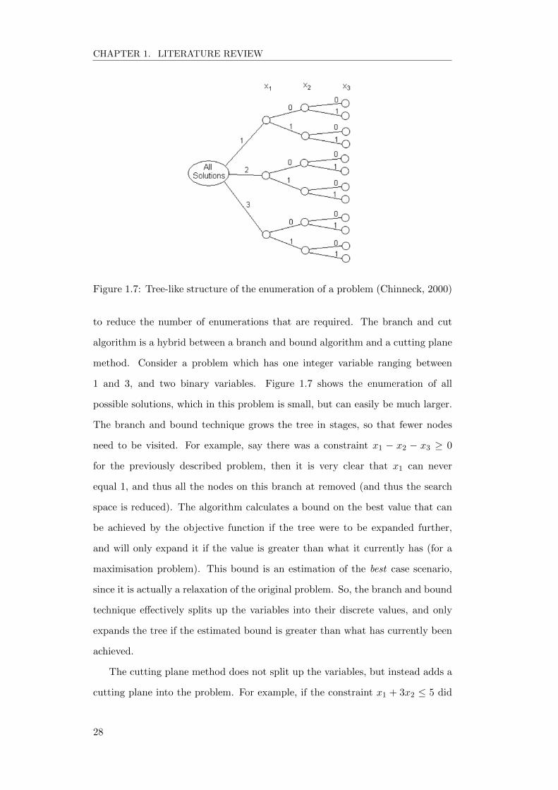
Figure 1.7: Tree-like structure of the enumeration of a problem (Chinneck, 2000)
to reduce the number of enumerations that are required. The branch and cut
algorithm is a hybrid between a branch and bound algorithm and a cutting plane
method. Consider a problem which has one integer variable ranging between
1 and 3, and two binary variables. Figure 1.7 shows the enumeration of all
possible solutions, which in this problem is small, but can easily be much larger.
The branch and bound technique grows the tree in stages, so that fewer nodes
need to be visited. For example, say there was a constraint x1 − x2 − x3 ≥ 0
for the previously described problem, then it is very clear that x1 can never
equal 1, and thus all the nodes on this branch at removed (and thus the search
space is reduced). The algorithm calculates a bound on the best value that can
be achieved by the objective function if the tree were to be expanded further,
and will only expand it if the value is greater than what it currently has (for a
maximisation problem). This bound is an estimation of the best case scenario,
since it is actually a relaxation of the original problem. So, the branch and bound
technique effectively splits up the variables into their discrete values, and only
expands the tree if the estimated bound is greater than what has currently been
achieved.
The cutting plane method does not split up the variables, but instead adds a
cutting plane into the problem. For example, if the constraint x1 + 3x2 ≤ 5 did
28
CHAPTER 1. LITERATURE REVIEW
not produce an integer feasible solution, the cutting plane method may choose to
change the constraint to x1 + 3x2 ≤ 4 and see if an integer solution is obtained
this time. A combination of both branching and cutting is what makes the B&C
algorithm powerful, and allows very large problems to be solved more easily.
There are many intricacies in the B&C algorithm, and it is up to the developer
of the algorithm to make it more efficient. The mathematical modeller should
be aware of how it works, but should not necessarily need to delve into the
details of its implementation. Colvin and Maravelias (2010) describe how they
developed a novel branch and cut algorithm which can reduce the time required
to obtain an optimal solution. It was applied to scheduling of clinical trials in
pharmaceutical research, and they illustrated that by understanding the real-
world problem they were able to adapt the algorithm to remove nodes from the
tree that were unnecessary, thus increasing speed. They mention that although
the methods were specific to a particular case, they could also be applicable to a
general class of problems.
1.4.3 Multi-objective methods
Most work involving capacity planning revolves around optimising single-objective
models. Usually the objective under consideration is total cost or net present
value (NPV). However, models which can incorporate multiple criteria are better
placed to provide more holistic manufacturing schedules which meet the various
conflicting objectives a biopharmaceutical company may have.
In terms of the stage at which a decision maker makes his/her preference,
there are three categories of multi-objective optimisation: the a priori methods,
the interactive methods and the a posteriori or generation methods (Hwang and
Masud, 1979). An example of a priori methods would include weighted-sum goal
programming, whereby a decision maker makes a preference prior to optimisation
by setting goals and weights in the objective function. The main issue with this
type of method is that it is difficult to determine beforehand which goal targets
and weights should be used. In the interactive methods, a decision maker reaches
the most preferred solution through dialogue with the multi-objective model. The
29

CHAPTER 1. LITERATURE REVIEW
search process will eventually converge to a solution that is most suitable given
the responses by the decision maker. However, this method prevents the user
from being able to see the entire decision space. In the a posteriori methods,
a complete set of efficient solutions is generated, and then the decision maker
selects the most suitable solution given his/her criteria.
There is extensive literature surrounding multi-objective optimisation of sup-
ply chain management. Amodeo et al. (2007) developed a simulation-based multi-
objective optimisation method for the inventory policies of supply chains. They
showed that their approach was able to obtain better solutions in terms of two
objectives: total inventory cost and service level. Roghanian et al. (2007) con-
sidered a probabilistic bi-level linear multi-objective programming problem and
applied fuzzy programming techniques adapted from Osman et al. (2004) to deal
with uncertain input parameters. As previously mentioned, Lakhdar et al. (2007)
incorporated multiple objectives, including cost, customer service level and ca-
pacity utilisation, into a biopharmaceutical capacity planning model via the use
of goal programming. Vahdani et al. (2012) developed a bi-objective mathemat-
ical programming formulation which minimizes the total costs and the expected
transportation costs after failure of facilities in a logistics network.
The ε-constraint method is an a posteriori method for multi-objective opti-
misation, and has been used in the context of supply chain management. Bashiri
et al. (2014) describe its use in a supply chain network for the objectives of cost
and customer satisfaction. The ε-constraint method was also used to generate
Pareto-optimal curves in a bi-criterion non-convex MINLP for the global optimi-
sation of chemical supply chains (Guillen and Grossmann, 2010). Pishvaee and
Razmi (2012) used the ε-constraint method to consider multiple environmental
impacts beside the traditional cost minimisation objective. Pozo et al. (2012)
use principal component analysis to reduce the number of objectives that need
to be considered within a chemical supply chain, and then use the ε-constraint
method to generate a set of Pareto solutions. Guillen et al. (2005) combined the
ε-constraint method with a two stage programming model to tackle the problem
of design and retrofit of a supply-chain network consisting of several production
30

CHAPTER 1. LITERATURE REVIEW
plants, warehouses, and markets, and the associated distribution systems. The
objectives considered were NPV, demand satisfaction and financial risk, with a
set Pareto of solutions generated to aid the decision maker. Mavrotas (2009)
presented a novel version of the ε-constraint method which avoided the genera-
tion of weakly Pareto optimal solutions and increases performance by removing
redundant iterations. The authors then improved the method with particular
attention to multi-objective integer problems (Mavrotas and Florios, 2013).
1.5 Alternative Heuristic Search Methods
Although formulating the problem using mathematical modelling allows for the
use of high performance solvers, sometimes the problem is too large to be solved
in reasonable time, and other times the problem is too complex to be described as
linear. In these cases, heuristic search methods can provide alternative methods
of arriving to an optimised solution. They may not be mathematically the best
solutions, but they can be very close to the optimal value, and the added benefit of
being able to model more complex situations with greater flexibility can outweigh
the downsides.
1.5.1 Simulated annealing
Simulated annealing is one of the older heuristic search methods (Metropolis
et al., 1953), and has been used for a variety of problems. Its name comes from
annealing in metals, whereby the metal is heated and then cooled down slowly,
thus increasing the size of its crystals and reducing their defects. The heat gives
the atoms energy to move away from their original positions (which can be clas-
sified as a local minimum of the internal energy) and move randomly through
states of higher energy; the slow cooling gives them more chance of finding con-
figurations with lower internal energy than the initial one. In combinatorial
optimisation, it works by searching through the entire problem space, preventing
itself from becoming trapped in a local optimum by allowing itself to move to
inferior solutions under certain conditions. Switching to an inferior solution is
31

CHAPTER 1. LITERATURE REVIEW
dependent on an acceptance probability function, which takes into account the
change in solution value (∆c), and temperature (T):
P () =
1 if ∆c > 0
e−∆cT if ∆c < 0
(1.1)
If P() is less than a uniform random number, R ∈ [0, 1], then a move to the
newly calculated solution will take place. Thus, if a solution is inferior to the
previously calculated solution, the algorithm may still change to it depending
on the probabilistic outcome of Equation 1.1. The temperature is reduced after
each iteration (T ← αT , where α is a constant close to 1), thus reducing the
chance of switching to an inferior solution as the iteration process goes on. The
initial temperature that is used is important, as this will determine how easily it
switches to inferior solutions at the beginning - starting with a low temperature
may result in becoming trapped in a local optima very quickly. Choosing an initial
temperature requires some knowledge of the problem, and can take trial an error
to get right. It should be noted that the number of iterations is dependent on
the initial temperature used, the α constant used to reduce the temperature, and
the final temperature (the temperature at which the process is stopped). The
final temperature is again somewhat problem dependent, but Lundy and Mees
proposed stopping when:
T ≤ ε
ln[(|S| − 1)/θ](1.2)
where S is the solution space, and the final solution is within ε of the optimum
with probability θ (Lundy and Mees, 1986).
Ku and Karimi (1991) showed one of the first applications of simulated an-
nealing in scheduling problems, and reported that out of the four algorithms that
they tried using, the simulated annealing algorithm provided the best solution,
although at the expense of greater CPU time when compared to their other iter-
ative algorithms. A similar result was obtained by Tandon et al. (1995), where
they showed that a simulated annealing algorithm provided better solutions than
32
CHAPTER 1. LITERATURE REVIEW
those given by other heuristic methods and the list scheduling algorithm. Their
approach incorporated sequence dependent clean-up times, and they measured
performance based on tardiness minimisation (i.e. ensuring products are deliv-
ered on time). There are examples of simulated annealing being used in computer
science, one being capacity planning of networks (Habib and Marimuthu, 2010).
They showed how the use of SA algorithms allowed them to cut network traffic by
20%, thereby increasing their overall network capacity and reducing maintenance
costs. Other work (Tsenov, 2006) showed how SA algorithms could be used to
optimise telecommunication networks by using different criteria such as network
reliability, restricting traffic congestion below a certain threshold, and respecting
a maximum transit time (the time for which a packet of information is travelling
through the network). In terms of biopharmaceutical manufacturing, this could
be interpreted as backlog delays, facility utilisation, and product shelf-life respec-
tively. Another example of SA being used is for the optimisation of investment
in a transportation network under uncertainty (Sun and Turnquist, 2007). The
model sought to maximise expected system capacity, subject to uncertainty of
future demand, and this had the effect of the model finding investment plans that
will create capacity flexibility as well as increasing expected capacity.
1.5.2 Genetic algorithms
Genetic algorithms (GA) are part of a branch of meta-heuristics called evolu-
tionary algorithms, termed as such because they derive much of their operating
characteristics from situations arising in biology. The technique for genetic al-
gorithms (Goldberg, 1989) starts by using a collection of solutions (known as a
population of chromosomes), and then using selective breeding and recombina-
tion strategies, better solutions are produced. Generally, the optimisation stops
when a certain number of generations have been produced, or when a satisfac-
tory solution has been reached. In terms of recombination, different numbers
of crossovers between chromosomes can be used to vary the offspring, and the
mutation rate can be varied too. Some studies have shown that having both a
higher mutation rate and different rates for different bits on the chromosomes
33

CHAPTER 1. LITERATURE REVIEW
can be beneficial; in fact it may also be useful to increase the mutation rate as
the search progresses.
Berning et al. (2004) have shown how genetic algorithms can be used for
supply chain optimisation in the chemical process industry. They describe how
the scheduling can be split up into two distinct parts: long-term planning which
look far ahead and provides a rough sketch of production capacity, and short-
term scheduling which considers production sequencing, keeping idle time and
inventory low, and all the other production constraints that are present. They
mention how mathematical modelling is often not the most ideal tool to use,
since many production constraints such as sequence dependencies and lot size
restrictions lead to NP -hard optimisation problems (Monma and Potts, 1989).
Recently, Ramteke and Srinivasan (2011) showed how GAs could be integrated
with a graph-based network structure so as to speed up the solution time. The
optimisation was concerning large-scale refinery crude-oil scheduling, where the
problem involved multiple objectives. They showed a significant reduction in
CPU time when compared to a standard MILP formulation, from 2988 seconds
to 34 seconds, with only a small decrease in profit for the GAs. Urselmann
et al. (2009) described the use of a hybrid algorithm, which they term a ‘memetic
algorithm’, which incorporates both GAs and local mathematical solvers. The
combination of the two optimisation methods reduced the overall search space,
and allowed for large global optimisation. The memetic algorithm exploits GAs’
ability to escape local optima, and uses a local NLP solver to optimise large
continuous problems locally. Together, these two methods gave a 75% increase
in speed in certain conditions when compared to an alternative algorithm called
OQNLP. This alternative algorithm is a scatter search based multi-start heuristic,
and works by generating multiple starting points from which a local NLP solver
(CONOPT in this case) starts its optimisation.
Estimation of Distribution Algorithms (EDAs), which are a branch of GAs,
have been used in a multi-objective optimisation framework, where the three
main criteria that were addressed were portfolio management, scheduling of drug
development and manufacturing, and whether or not third parties should be used
34

CHAPTER 1. LITERATURE REVIEW
for manufacturing or development of candidate drugs (George and Farid, 2008a).
The model built upon previous work (George et al., 2007) where simulation was
used in a multi-criteria decision-making framework to aid companies when faced
with the acquisition of commercial-scale biopharmaceutical manufacturing ca-
pacity. The detailed economic model from this work, alongside with the genetic
algorithms added in the optimisation framework, allowed George and Farid to
show that by taking multiple drug candidates into consideration rather than just
one single drug, the overall risk to NPV can be reduced, although one of the side
effects of reducing NPV risk is that the overall mean NPV is reduced. The results
suggested the integration of all activities in-house in scenarios without budgetary
constraints. However, in scenarios with budgetary constraints, the results indi-
cated that managing risk through outsourcing to CMOs and sharing capacity
with partners would be a more optimal strategy. Hence, the optimization out-
puts propose committing to creating capacity as late as possible with limited
budgetary constraints. However, the key point of the work was that an opti-
misation framework, using evolutionary algorithms and machine learning, had
been used to solve portfolio development and capacity planning simultaneously,
something which had not been done before.
1.5.3 Swarm intelligence
Swarm intelligence is a branch of artificial intelligence which takes ideas from
behaviour prevalent amongst social insects or animal societies, and applies them
to the design of multi-agent systems. Techniques using swarm intelligence for op-
timisation have recently become popular, largely due to their ability to deal with
complex problems in a robust and flexible manner. Two of the more successful
techniques are ant colony optimisation and particle swarm optimisation, the first
of which will be discussed here. The use of ant colony optimisation (ACO) in
combinatorial optimisation was first described by Dorigo et al. (1991), the inspi-
ration of which came from observing how ants forage for food. Figure 1.8 shows
a summary of how ant foraging works.
A good explanation of how ant foraging can be applied to optimisation prob-
35

CHAPTER 1. LITERATURE REVIEW
Figure 1.8: Shortest path find by an ant colony (Dreo, 2006). Ants can followany of the four routes from the nest (N) to the food source (F). As they return tothe nest, they lay a pheromone trail. The ant which took the shortest route willreturn first, and thus the probability of the shorter path having more pheromone(which influences the ants’ decision on which path to take) will be higher. Thenet effect is that over time, almost all the ants will follow the shorter path.
lems can be found in paper by Blum and Li (2008), where they outline a frame-
work that can be used to solve the travelling salesman problem (TSP). Compared
to other state-of-the-art techniques, the original ACO algorithm was not as good
at solving the TSP, and thus different variants of the ACO framework came into
existence, mainly varying in the rules applied to pheromone update (Dorigo, 1992;
Dorigo and Gambardella, 1997; Stutzle and Hoos, 2000). ACO has been applied
to a number of problem types, including bioinformatics (Shmygelska et al., 2002),
scheduling (Merkle et al., 2000), multi-objective problems (Guntsch and Midden-
dorf, 2003), and dynamic problems (Guntsch and Middendorf, 2001). One of
the problems with ACO is that when a problem becomes highly constrained (for
example, in scheduling problems), ACO performance is inferior to other meth-
ods of optimisation. This is also seen with other search heuristics, the reason
being that when a problem in not excessively constrained, the hard part becomes
36

CHAPTER 1. LITERATURE REVIEW
optimisation rather than finding a feasible solution. In these instances, ACO al-
gorithms and other meta-heuristic algorithms perform well. However, when the
problem is very constrained, the difficulty lies in finding feasible solutions rather
than the optimisation. Restricting the search space to promising regions is part
of something called constraint programming, and has been hybridised with ACO
to enable its use to more challenging problems (Meyer and Ernst, 2004). Wang
and Chen (2009) developed an ant algorithm that can solve non-linear mixed in-
teger programming models which maximise profit through capacity planning and
resource allocation. They used constraint programming techniques mentioned
previously to deal with the problem’s inherent complexities, and found that the
solutions provided by the algorithm were equal to that of genetic algorithms.
1.6 Justification of Mathematical Programming Ap-
proach
This work focuses on MILP methods to determine optimal manufacturing sched-
ules. Other methods have been highlighted in this literature review, but none
provide the proof that a solution is globally optimal. Furthermore, bioman-
ufacturing capacity plans have not been researched extensively using heuristic
methods, whereas encouraging attempts have already been made in mathemati-
cal programming. Whilst literature for mathematical techniques in biomanufac-
turing are limited, there is extensive research that has been conducted in other
sectors for the case of capacity planning. Other techniques can also be inves-
tigated in tandem, but they should ultimately be compared to exact methods,
hence this thesis predominately focuses on MILP methods.
1.7 Aims and Organisation of Thesis
The previous sections have described the main issues the biopharmaceutical in-
dustry are currently facing, and how these pressures influence decisions regarding
capacity planning. Optimisation techniques addressing how capacity planning
37
CHAPTER 1. LITERATURE REVIEW
challenges have been solved in other industries have been discussed. Mathemat-
ical techniques such as mixed integer linear programming and alternative search
heuristics such as genetic algorithms have been investigated in the context of
biopharmaceutical capacity planning. Despite the attention that has been given
to this problem domain in literature, cases where both perfusion and fed-batch
processes are present have not been considered. As manufacturers start to see the
benefits of using perfusion systems, there will be a greater need for optimisation
models that can cater for these processes.
The aim of this thesis is to develop a computational decision tool which can
provide biomanfacturing production plans for different modes of cell culture. In
particular, it should provide:
• Modelling of perfusion mode and fed-batch mode cell cultures
• Manufacturing schedules for long-term planning horizons
• Biomanfacturing costs and capital investment profiles
• Optimal selection of capacity expansion options
• Analysis and optimisation surrounding multi-criteria strategic decision mak-
ing
• Analysis of the impact of uncertainty on biopharmaceutical capacity plan-
ning
The aim of this thesis is therefore to create a framework that produces optimal
solutions to biopharmaceutical capacity planning problems, considering various
capacity expansion options and different product types. The remainder of this
thesis is structured around achieving these aims.
Chapter 2 discusses the problem domain in greater detail, including the
model’s input requirements and expected outputs. The need for an automated
decisional tool is highlighted by an illustration of the computational complex-
ity of the problem. Finally, an overview of how the framework is constructed is
presented.
38

CHAPTER 1. LITERATURE REVIEW
Chapter 3 outlines the challenges present in biopharmaceutical manufacturing
when both perfusion and fed-batch processes must be considered. A discrete-time
mixed integer linear program is created which accurately models both perfusion
and fed-batch processes to produce optimal capacity plans. Sequence-dependent
changeovers are introduced to correctly model the increased time required to
switch between different process modes. To improve computational performance,
a rolling time horizon is implemented.
The performance of the mathematical model is improved further in Chapter
4. A state task network (STN) representation is used to reduce the number of
constraints and variables in the model, and improve computational efficiency and
solution quality. The performance of the STN model is tested on two industrial
case studies. New features are also added to the model, to further increase realism
of the manufacturing schedules.
Chapter 5 discusses the addition of a multi-objective component to the STN
model. Two methods are compared, weighted-sum goal programming and the
ε-constraint method. The multi-criteria nature of biopharmaceutical capacity
planning is explored via the consideration of various strategic objectives. An
analysis of the impact these considerations can have on manufacturing schedules,
capital expenditure and risk is discussed.
Chapter 6 outlines the important conclusions of this work, and possible av-
enues of extending the framework. Finally, Appendix B lists papers of the author
published during the course of this work.
39

CHAPTER 1. LITERATURE REVIEW
40

Chapter 2
Requirements and Analysis
This section will outline the problem being solved in more detail. It will discuss
why the problem needs to be addressed, what information is required in order
to solve the problem, and what exactly should be expected from the decision-
support tool being developed. Finally, the components of the framework and
how they work together are discussed.
2.1 Detailed Problem Statement
In order to reduce costs, biopharmaceutical manufacturers would like more guid-
ance and assistance in decision-making regarding strategic planning. In terms of
capacity planning, they would like to know when and where they should manu-
facture a product. This is simple for cases involving a small number of products
in their portfolios, with one or two manufacturing facilities to choose from. How-
ever, as the number of products and facilities increases, so does the complexity of
the problem, becoming much more difficult to solve manually. In order to better
understand the problem, it is first necessary to discuss some of the constraints
and inputs which influence the decision-making.
First of all, a list of the products and facilities that are to be included in the
model need to be analysed. Different products will have distinct modes of cell
culture (for example, fed-batch or perfusion mode). Facilities will also have their
own capabilities regarding which products they can manufacture (see Figure 2.1).
41

CHAPTER 2. REQUIREMENTS AND ANALYSIS
Secondly, some information regarding the process needs to be ascertained. For a
more detailed and complex model, information on the individual unit processes
would be needed, but if the model is to assume a black box approach, then just
the overall output information is required. For example, this could include data
akin to the output of each batch (in kilograms), the time it takes to produce one
batch, and the cost of manufacturing each batch. Then, using demand targets,
one can begin working out which product needs to be produced where.
DSPUSP
Market
DSPUSP
USP suites: 2
DSP suites: 2
(a)
DSPUSP
Market
DSPUSP
USP suites: 2
DSP suites: 1
(b)
DSPUSP
Market
DSPUSP
USP suites: 1
DSP suites: 2
(c)
Figure 2.1: Capability matrices for a network of two USP suites and two DSP
suites. The number of suites available for use for a particular product is shown
on the left. In (a) both USP and DSP suites are available, in (b) only one DSP
suite can be used, and in (c) only one USP suite is available.
The problem becomes more complicated when other factors are considered,
such as product shelf-life (the product cannot be stored indefinitely but must
be sold before it expires), an individual facility’s storage capacity, and sequence
dependent changeover times (Figure 2.2). The time required to switch between
products includes the time to clean the suite and also move any equipment,
and thus will depend on the equipment the processes use. Therefore, sequence
dependent changeover times are required when the model contains vastly different
product types. There are also options to manufacture in a CMO, or build a future
42

CHAPTER 2. REQUIREMENTS AND ANALYSIS
facility to cope with future demand. In fact, some facilities can also be retrofitted
so that they are able to manufacture other products, again making the problem
more complex. Figure 2.3 shows an overall view on some of the aspects which
can be included in the model.
P1 P2
Time
No changeovers
Fixed changeovers
P3
P1 P2 P3
Sequence dependent
changeoversP1 P2 P3
Figure 2.2: Different methods of modelling changeover times between products
The mathematical model must be realistic in order for the results to be mean-
ingful. It must try as closely as possible to mimic what would happen in practice,
and thus different versions of the model will be developed as the model evolves in
complexity. For the simple case, the whole process (both USP and DSP) can be
treated as a black box (Siganporia et al., 2012). However, one of the key limita-
tions of that model is the lack of manufacturing flexibility from coupling upstream
and downstream processes to one another. One reason why it is beneficial to de-
couple upstream and downstream production is because for perfusion processes,
manufacturers often completely separate the upstream and downstream process,
freezing the intermediate product in between. Allowing the USP and DSP to be
modelled separately permits products to be manufactured alongside each other
within the same facility, which would not have been possible with a simple black
box design.
In theory, the material produced upstream in one facility can be processed
downstream in a completely different facility, and thus the model can be adapted
for this scenario too.
43
CHAPTER 2. REQUIREMENTS AND ANALYSIS
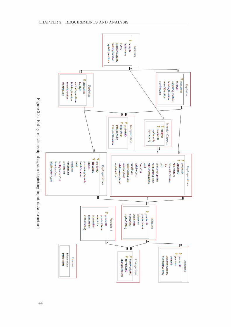
Fig
ure
2.3:E
ntity
relationsh
ipd
iagramd
epictin
gin
pu
td
atastru
cture
44

CHAPTER 2. REQUIREMENTS AND ANALYSIS
Figure 2.4: Separating USP from DSP. Note that this assumes that there wasalready some intermediate product stored for product 2.
2.2 Computational Complexity
To create a capacity plan manually, taking all these constraints into consideration,
is a very difficult task - but not impossible. The dilemma is that any solution
that is found manually is extremely unlikely to be optimal, and in the case of
multi-billion dollar biopharmaceutical companies, any sub-optimal solution could
be costing them a huge amount in losses. The need for a decision-support tool
becomes even more evident when one examines a small test case:
Imagine there are two facilities (i) and two products (p), and that there is a
demand for both products at some time in the future. In any given time period,
the possible solutions are:
1. p1 is produced in i1
2. p1 is produced in i2
3. p2 is produced in i1
4. p2 is produced in i2
5. p1 is produced in i1 AND p1 is produced in i2
6. p2 is produced in i1 AND p2 is produced in i2
7. p1 is produced in i1 AND p2 is produced in i2
8. p2 is produced in i1 AND p1 is produced in i2
9. No production in either i1 or i2
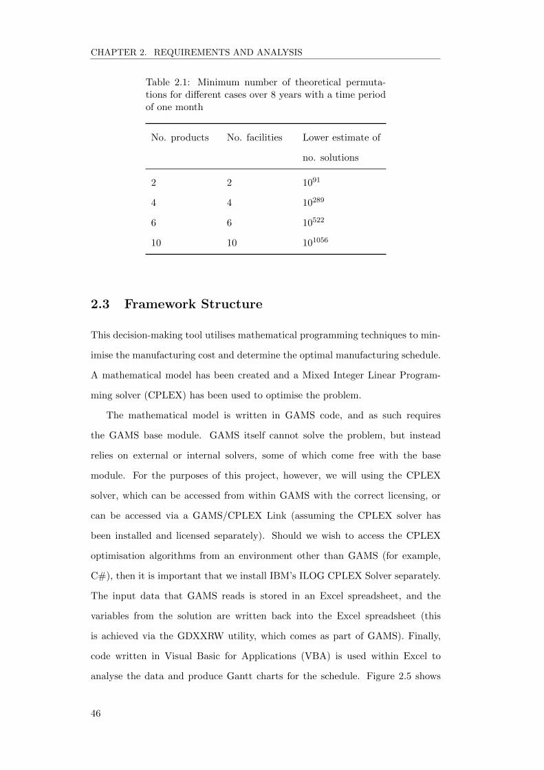
Bearing in mind that this is just for one time period, it becomes easy to
see that with a greater number of products and facilities, the problem becomes
exponentially more difficult to solve (see Table 2.1).
45
CHAPTER 2. REQUIREMENTS AND ANALYSIS
Table 2.1: Minimum number of theoretical permuta-tions for different cases over 8 years with a time periodof one month
No. products No. facilities Lower estimate of
no. solutions
2 2 1091
4 4 10289
6 6 10522
10 10 101056
2.3 Framework Structure
This decision-making tool utilises mathematical programming techniques to min-
imise the manufacturing cost and determine the optimal manufacturing schedule.
A mathematical model has been created and a Mixed Integer Linear Program-
ming solver (CPLEX) has been used to optimise the problem.
The mathematical model is written in GAMS code, and as such requires
the GAMS base module. GAMS itself cannot solve the problem, but instead
relies on external or internal solvers, some of which come free with the base
module. For the purposes of this project, however, we will using the CPLEX
solver, which can be accessed from within GAMS with the correct licensing, or
can be accessed via a GAMS/CPLEX Link (assuming the CPLEX solver has
been installed and licensed separately). Should we wish to access the CPLEX
optimisation algorithms from an environment other than GAMS (for example,
C#), then it is important that we install IBM’s ILOG CPLEX Solver separately.
The input data that GAMS reads is stored in an Excel spreadsheet, and the
variables from the solution are written back into the Excel spreadsheet (this
is achieved via the GDXXRW utility, which comes as part of GAMS). Finally,
code written in Visual Basic for Applications (VBA) is used within Excel to
analyse the data and produce Gantt charts for the schedule. Figure 2.5 shows
46

CHAPTER 2. REQUIREMENTS AND ANALYSIS
the architecture of the framework, and gives examples of the type of data or
actions that link components together.
Figure 2.5: System Design
One of the drawbacks of using Excel as the input for GAMS is that editing
spreadsheets when changing case studies is a tedious and error-prone process.
GAMS must read data as matrices, thus if the number of products or facilities
change, the size of the tables in Excel also change, leading to scaling issues. Thus
the data was also converted to a relational database format, thereby increasing
scalability and ease of use. The entity relationship diagram shown in Figure 2.3
demonstrates how the tables within the database are linked to each other. This
change in input format was not completed in time to be incorporated into the
framework described here, but it was used in a separate model which used genetic
algorithms to optimise production plans. This is explained in more detail later.
2.4 Model Requirements
Having explained the problem in more detail, and how the framework components
are structured, it is now necessary to outline what functionality the framework
47
CHAPTER 2. REQUIREMENTS AND ANALYSIS
should be expected to provide. The following are some requirements:
• Gantt chart showing the production schedule
• Number of batches and hence material output per time period
• Facility utilisation
• Customer service level
• COGS
• Capital expenditure
• Net present value
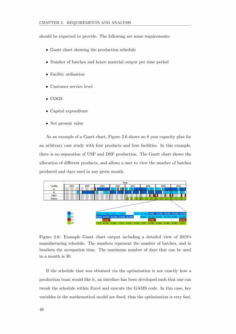
As an example of a Gantt chart, Figure 2.6 shows an 8 year capacity plan for
an arbitrary case study with four products and four facilities. In this example,
there is no separation of USP and DSP production. The Gantt chart shows the
allocation of different products, and allows a user to view the number of batches
produced and days used in any given month.
Figure 2.6: Example Gantt chart output including a detailed view of 2019’s
manufacturing schedule. The numbers represent the number of batches, and in
brackets the occupation time. The maximum number of days that can be used
in a month is 30.
If the schedule that was obtained via the optimisation is not exactly how a
production team would like it, an interface has been developed such that one can
tweak the schedule within Excel and execute the GAMS code. In this case, key
variables in the mathematical model are fixed, thus the optimisation is very fast,
48

CHAPTER 2. REQUIREMENTS AND ANALYSIS
and acts more like an infeasibility checker. This flexibility can help in instances
where there is a bias to manufacturing in a certain way, but where cost is not
affected (and hence is not considered in the mathematical model).
2.5 Summary
This chapter has described in more detail the problem being tackled by this
decision-support tool. The usefulness of a tool that will aid strategic planning for
future products is undoubtedly high, and can enable a company to better predict
likely cash outflows owing to capital investment. Uncertainty can be incorporated
via running different scenarios, and can help identify more robust manufacturing
strategies, and thereby help contain risk.
In the next chapter, a description of the mathematical model is outlined,
with results showing how the tool was used on an industrial case study to help
determine optimal manufacturing schedules.
49

CHAPTER 2. REQUIREMENTS AND ANALYSIS
50

Chapter 3
Capacity planning for batch
and perfusion bioprocesses
across multiple
biopharmaceutical facilities
3.1 Introduction
Biopharmaceutical companies with growing portfolios of commercial therapeu-
tics face the challenge of generating medium and long-term production plans
for several drugs across several multi-product manufacturing sites that maximise
capacity whilst minimising cost.
Production planning is complicated by portfolios of commercial candidates
that are made with different cell culture modes: fed-batch mode, or continuous
perfusion for labile products. The complication arises from the fact that perfusion
cell cultures can span many months, whereas fed-batch cell cultures are usually
two weeks in duration. The discrete time representation used in this model is
of one month, thus extra modelling constraints need to be introduced to ensure
that production is not stopped half-way through a cell culture (since it is meant
to model a continuous process). Every time a new perfusion cell culture begins,
51

CHAPTER 3. CAPACITY PLANNING FOR BATCH AND PERFUSIONBIOPROCESSES ACROSS MULTIPLE BIOPHARMACEUTICAL FACILITIES
ramp-up times need to be considered, since the manufacturer may choose not
to harvest any material during this period, due to it not meeting all required
specifications. Material is normally harvested semi-continuously from perfusion
processes, which is conceptually different from a fed-batch process where material
is harvested at the end of the cell culture. Thus these continuous harvests need to
be incorporated in the model’s constraints. Changing from one mode of operation
to another also increases the changeover time normally associated with product
switchovers. This adds more complexity to the optimisation since a larger number
of constraints is required.
This chapter describes the development of a discrete-time mixed integer linear
programming (MILP) model that incorporates both perfusion and fed-batch pro-
cesses to produce capacity plans and manufacturing schedules. Extra constraints
have been incorporated to more realistically model the perfusion process. For
example, ramp-up times and cell culture durations spanning multiple time peri-
ods have been implemented for perfusion-mode processes. One of the challenges
met by this formulation is the ability to include sequence-dependent changeover
times between products, which is necessary because switching between perfusion
and fed-batch modes takes longer than staying within the same process mode.
Annual fixed costs are also included in the model, along with other investment
considerations such as retrofitting costs and investment into constructing new
facilities. These additional features allow the model to pick strategies based on
a more holistic approach, and thus provide more economically feasible solutions.
Strategic inventory targets have also been implemented such that the manufac-
turer can choose to have extra stock of product should demand unexpectedly
rise or supply suddenly fall. These extra features add to the complexity of the
model, and thus require additional CPU resources in order to obtain a satis-
factory solution. Hence a rolling time horizon has been implemented and has
successfully managed to improve solutions, whilst at the same time reduce CPU
requirements. The impact of variations on key parameters such as demand or
titres on the optimal production plans and costs was captured through scenario
analysis.
52

CHAPTER 3. CAPACITY PLANNING FOR BATCH AND PERFUSIONBIOPROCESSES ACROSS MULTIPLE BIOPHARMACEUTICAL FACILITIES
The remainder of this chapter consists of an explanation of the problem do-
main in Section 3.2, followed by a description of the mathematical formulation
used in the MILP model in Section 3.3. An industrial case study is then used
to explore the capabilities of the model and identify trends which can be used to
aid business decisions. The mathematical nomenclature can be found at the end
of this paper.
3.2 Problem Definition
The focus of this work is on long-term multi-site production planning for bio-
pharmaceuticals to minimise the total manufacturing cost and investment whilst
satisfying demands. The key features of the problem are discussed below.
3.2.1 Facility features
Allocation of biopharmaceutical facilities across multiple sites requires an under-
standing of the different facility features such as scale and capability to manu-
facture each product as well as any differences in fermentation titres and down-
stream processing yields. The number and size of bioreactors will directly affect a
facility’s upstream processing (USP) capacity. The same product could be man-
ufactured in two different facilities, with each facility having a different number
of bioreactors available, hence the optimisation will select which facility to use
based on cost and capacity requirement. Downstream processing (DSP) scales
will also vary, since there may be different sized purification equipment such as
chromatography columns or filtration rigs. Depending on how the DSP is set up,
it could mean that the time required for purification is different between facilities.
For example, if the same amount of material is to be processed by a facility with a
smaller filtration device, that particular step will be slower (when compared to a
larger filtration unit with greater throughput). There may also be multiple DSP
trains to process the material from one harvest, which is common for antibody
production with high titres (Kelley, 2009). On the other hand, operators could
decide to keep the purification time constant, but change the amount of material
53

CHAPTER 3. CAPACITY PLANNING FOR BATCH AND PERFUSIONBIOPROCESSES ACROSS MULTIPLE BIOPHARMACEUTICAL FACILITIES
processed. These process choices must be correctly captured in the model for
there to be realistic manufacturing flexibility.
The capability of a facility to manufacture a product will differ, not just owing
to logistical aspects, but also strategic. For example, if a future facility is built
with perfusion products in mind, then it may not be possible to later manufacture
fed-batch products. A CMO however, may be capable of manufacturing all of
the products, but due to licensing and IP issues a company may wish to keep
production of certain products in-house. Another key facility feature is the cost
of manufacturing a product there. Cost differences are present between in-house
and CMO facilities to reflect the extra service cost with CMOs (George and Farid,
2008b).
3.2.2 Fed-batch versus perfusion culture processes
The USP stages of mammalian cell culture processes typically involve either fed-
batch or perfusion culture (Pollock et al., 2013). It is also possible to have one or
more steps of the seed train as perfusion-mode, and the production cell culture
as fed-batch (Pohlscheidt et al., 2013). Perfusion culture is necessary for labile
products such as blood factors and enzymes (e.g., Cerezyme) and has also been
used for certain stable monoclonal antibody (mAb) products (e.g., Remicade) us-
ing retention devices that range from gravity settlers to filtration devices (Pollock
et al., 2013). Perfusion processes typically offer higher daily volumetric produc-
tivities and hence smaller facility footprints than fed-batch culture strategies.
However, they are generally more complex to operate, require increased amounts
of media, and are susceptible to higher failure rates (Cacciuttolo, 2007). Newer
perfusion retention devices using external tangential flow filters aim to overcome
some of these obstacles with the capability to attach to single-use bioreactors
combined with lower failure rates and higher productivities (Clincke et al., 2013).
This has increased interest in the business case for perfusion-based processes and
process economic analyses have explored the cost-benefit of perfusion versus fed-
batch processes.23, 25 However, in recent years, fed-batch culture has become
the platform choice for most mAbs due to dramatic increases in fed-batch titres
54
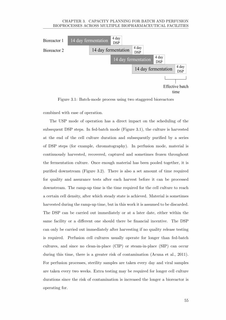
CHAPTER 3. CAPACITY PLANNING FOR BATCH AND PERFUSIONBIOPROCESSES ACROSS MULTIPLE BIOPHARMACEUTICAL FACILITIES
14 day fermentation 4 dayDSP
Bioreactor 1
14 day fermentation 4 dayDSPBioreactor 2
14 day fermentation 4 dayDSP
14 day fermentation 4 dayDSP
Effective batchtime
Figure 3.1: Batch-mode process using two staggered bioreactors
combined with ease of operation.
The USP mode of operation has a direct impact on the scheduling of the
subsequent DSP steps. In fed-batch mode (Figure 3.1), the culture is harvested
at the end of the cell culture duration and subsequently purified by a series
of DSP steps (for example, chromatography). In perfusion mode, material is
continuously harvested, recovered, captured and sometimes frozen throughout
the fermentation culture. Once enough material has been pooled together, it is
purified downstream (Figure 3.2). There is also a set amount of time required
for quality and assurance tests after each harvest before it can be processed
downstream. The ramp-up time is the time required for the cell culture to reach
a certain cell density, after which steady state is achieved. Material is sometimes
harvested during the ramp-up time, but in this work it is assumed to be discarded.
The DSP can be carried out immediately or at a later date, either within the
same facility or a different one should there be financial incentive. The DSP
can only be carried out immediately after harvesting if no quality release testing
is required. Perfusion cell cultures usually operate for longer than fed-batch
cultures, and since no clean-in-place (CIP) or steam-in-place (SIP) can occur
during this time, there is a greater risk of contamination (Acuna et al., 2011).
For perfusion processes, sterility samples are taken every day and viral samples
are taken every two weeks. Extra testing may be required for longer cell culture
durations since the risk of contamination is increased the longer a bioreactor is
operating for.
55
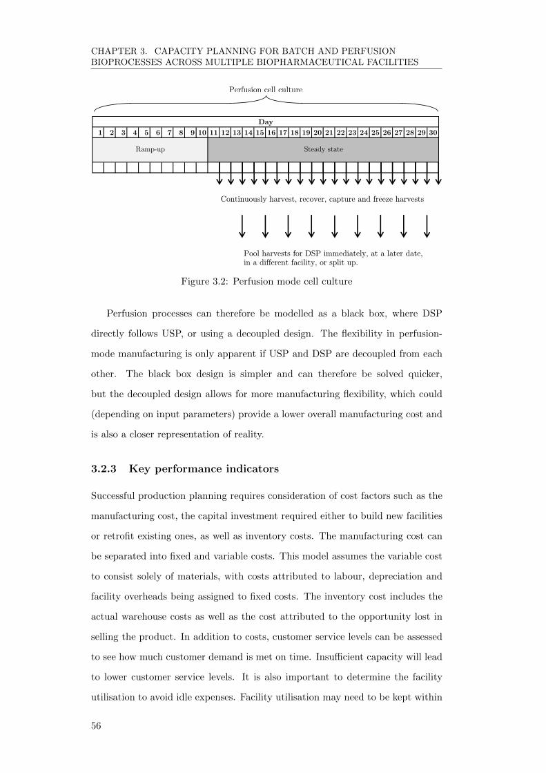
CHAPTER 3. CAPACITY PLANNING FOR BATCH AND PERFUSIONBIOPROCESSES ACROSS MULTIPLE BIOPHARMACEUTICAL FACILITIES
1 2 3 4 5 6 7 8 9 10 11 12 13 14 15 16 17 18 19 20 21 22 23 24 25 26 27 28 29 30
Continuously harvest, recover, capture and freeze harvests
Day
Pool harvests for DSP immediately, at a later date, in a different facility, or split up.
Perfusion cell culture
Ramp-up Steady state
Figure 3.2: Perfusion mode cell culture
Perfusion processes can therefore be modelled as a black box, where DSP
directly follows USP, or using a decoupled design. The flexibility in perfusion-
mode manufacturing is only apparent if USP and DSP are decoupled from each
other. The black box design is simpler and can therefore be solved quicker,
but the decoupled design allows for more manufacturing flexibility, which could
(depending on input parameters) provide a lower overall manufacturing cost and
is also a closer representation of reality.
3.2.3 Key performance indicators
Successful production planning requires consideration of cost factors such as the
manufacturing cost, the capital investment required either to build new facilities
or retrofit existing ones, as well as inventory costs. The manufacturing cost can
be separated into fixed and variable costs. This model assumes the variable cost
to consist solely of materials, with costs attributed to labour, depreciation and
facility overheads being assigned to fixed costs. The inventory cost includes the
actual warehouse costs as well as the cost attributed to the opportunity lost in
selling the product. In addition to costs, customer service levels can be assessed
to see how much customer demand is met on time. Insufficient capacity will lead
to lower customer service levels. It is also important to determine the facility
utilisation to avoid idle expenses. Facility utilisation may need to be kept within
56

CHAPTER 3. CAPACITY PLANNING FOR BATCH AND PERFUSIONBIOPROCESSES ACROSS MULTIPLE BIOPHARMACEUTICAL FACILITIES
certain targets. If facility utilisation is too high, any unplanned downtime could
severely affect the customer service level. Under-utilisation, on the other hand,
may suggest a misplaced investment in capacity. Together, these performance
indicators help a manufacturer to assess the viability of a production plan.
3.3 Mathematical formulation and solution procedure
The following section describes the mathematical formulation developed to ad-
dress the problem domain. The nomenclature can be found at the end of this
chapter. It is important to note that many of the variables have been duplicated
for the upstream and downstream parts of the model (for example, the number
of batches produced). To aid with legibility, the superscripts ‘U’ or ‘D’ denote
upstream or downstream respectively. This model uses a discrete time represen-
tation, with monthly time resolution. This means, for example, that for an eight
year planning horizon there would be 96 time periods. One of the assumptions
made in this model is that only one product can be produced in any given time
period. This can be justified by the fact that for biopharmaceutical manufac-
turing, it is unlikely that there is going to be a high rate of switching between
products (owing to quality, control, and logistic issues that may arise). So as long
as the time periods are relatively small, this limitation of one product per time
period should be of no concern. This model uses monthly time periods, hence
there should be no issue. Indeed, all the perfusion products in the case study
have fermentation cell cultures which last at least than one month, thus are not
affected by this limit. One of the reasons this assumption was made was because
it made it easier to model the scheduling of the problem, with less computational
effort required.
3.3.1 Technical and commercial constraints
Production constraints
In essence, the number of upstream batches produced in time period t, for prod-
uct p, in fermentation suite i, is denoted by BUipt and is equal to the batch rate
57

CHAPTER 3. CAPACITY PLANNING FOR BATCH AND PERFUSIONBIOPROCESSES ACROSS MULTIPLE BIOPHARMACEUTICAL FACILITIES
(rUip) multiplied by the amount of time available (TUipt). If there is a changeover
between products p′ and p, ZUip′pt will equal 1, and a campaign changeover time
(αp′p) is subtracted from the available time. Depending on whether the product
is manufactured using fed-batch or perfusion culture, an additional time is sub-
tracted. For perfusion products p ∈ P p (Equation 3.1), the ramp-up times (βp)
are subtracted when new perfusion cell cultures begin (Fipt = 1). For fed-batch
products p /∈ P p (Equation 3.2), the time required for the first batch (τ ′p) is
subtracted so that the effective batch rate can be used from that point onwards.
For example, if the fed-batch process is like that shown in Figure 3.1, the first
upstream batch would take 14 days, but from that point onwards there will be
another batch every 7 days. The extra time necessary for the first batch is only
required when a new campaign starts (Y ′ipt = 1). To compensate for the removal
of time for the first batch, Y ′ipt is added to the number of batches. Hence, when a
new campaign of a fed-batch product begins, Y ′ipt is equal to 1, and the number
of batches produced is equal to 1 plus the effective batch rate multiplied by time
available minus time required for the first batch.
BUipt = rUip(T
Uipt − βpFipt −
∑p′
αp′pZUip′pt) ∀t, p ∈ P p, i ∈ It ∩ Ip (3.1)
BUipt = Y ′ipt + rUip(T
Uipt − τ ′pY ′ipt −
∑p′
αp′pZUip′pt) ∀t, p /∈ P p, i ∈ It ∩ Ip
(3.2)
To ensure only one product is manufactured in a suite at any given time, the
binary variables Y Uipt and Y D
ipt, which are equal to 1 if product p is manufactured in
suite i at time t for upstream and downstream suites respectively, are constrained
as follows:
∑p
Y Uipt ≤ 1 ∀ t, i ∈ It (3.3)
58
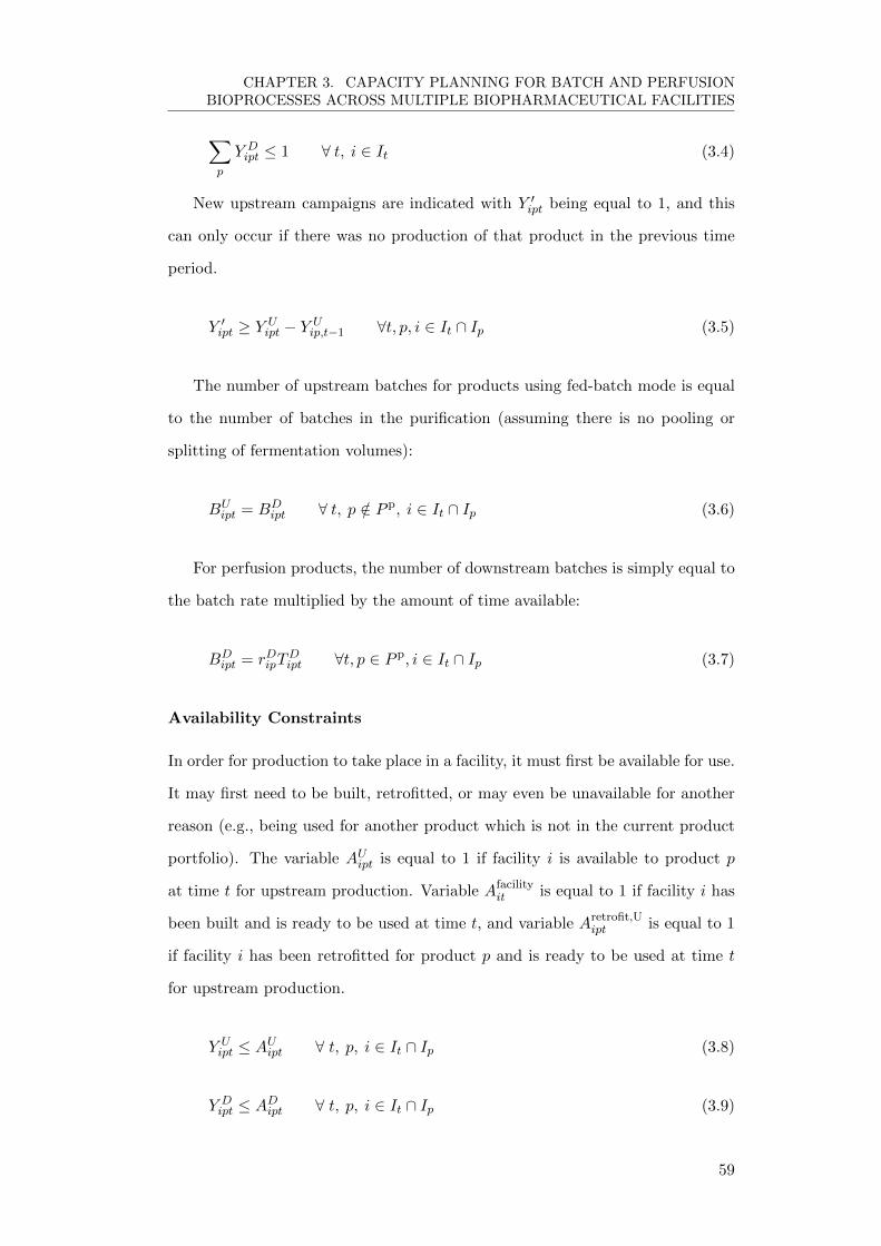
CHAPTER 3. CAPACITY PLANNING FOR BATCH AND PERFUSIONBIOPROCESSES ACROSS MULTIPLE BIOPHARMACEUTICAL FACILITIES
∑p
Y Dipt ≤ 1 ∀ t, i ∈ It (3.4)
New upstream campaigns are indicated with Y ′ipt being equal to 1, and this
can only occur if there was no production of that product in the previous time
period.
Y ′ipt ≥ Y Uipt − Y U
ip,t−1 ∀t, p, i ∈ It ∩ Ip (3.5)
The number of upstream batches for products using fed-batch mode is equal
to the number of batches in the purification (assuming there is no pooling or
splitting of fermentation volumes):
BUipt = BD
ipt ∀ t, p /∈ P p, i ∈ It ∩ Ip (3.6)
For perfusion products, the number of downstream batches is simply equal to
the batch rate multiplied by the amount of time available:
BDipt = rDipT
Dipt ∀t, p ∈ P p, i ∈ It ∩ Ip (3.7)
Availability Constraints
In order for production to take place in a facility, it must first be available for use.
It may first need to be built, retrofitted, or may even be unavailable for another
reason (e.g., being used for another product which is not in the current product
portfolio). The variable AUipt is equal to 1 if facility i is available to product p
at time t for upstream production. Variable Afacilityit is equal to 1 if facility i has
been built and is ready to be used at time t, and variable Aretrofit,Uipt is equal to 1
if facility i has been retrofitted for product p and is ready to be used at time t
for upstream production.
Y Uipt ≤ AUipt ∀ t, p, i ∈ It ∩ Ip (3.8)
Y Dipt ≤ ADipt ∀ t, p, i ∈ It ∩ Ip (3.9)
59

CHAPTER 3. CAPACITY PLANNING FOR BATCH AND PERFUSIONBIOPROCESSES ACROSS MULTIPLE BIOPHARMACEUTICAL FACILITIES
AUipt ≤ Afacilityit ∀ t, p, i ∈ It ∩ Ip (3.10)
ADipt ≤ Afacilityit ∀ t, p, i ∈ It ∩ Ip (3.11)
AUipt ≤ Aretrofit,Uipt ∀ t, p, i ∈ It ∩ Ip (3.12)
ADipt ≤ Aretrofit,Dipt ∀ t, p, i ∈ It ∩ Ip (3.13)
The availabilities for building a facility or retrofitting (Afacilityit , Aretrofit,U
ipt ) are
linked to the investment constraints which follow.
Investment Constraints
Before a facility can be used, there must first be investment into the construction
of that facility. The facility is not available before the time is takes to construct
it (τbuildi ). Construction starts as soon as investment is made. The variable Kit
is equal to 1 if capital is invested at time t.
Afacilityit ≤ Afacility
i,t−1 +Ki,t−τbuildi
∀ i, t (3.14)
In order for a product to be manufactured in a facility, any relevant retrofitting
must be carried out. LUipt is equal to 1 if facility i has been retrofitted for product
p at time t. The investment for retrofitting must be spent τ retrofiti time periods
before the facility becomes available for that product.
Aretrofit,Uipt ≤ Aretrofit,U
ip,t−1 + LUip,t−τ retrofit
i∀ t, p, i ∈ It ∩ Ip (3.15)
Aretrofit,Dipt ≤ Aretrofit,D
ip,t−1 + LDip,t−τ retrofit
i∀ t, p, i ∈ It ∩ Ip (3.16)
The model also includes any licence fees and start-up costs, and this is in-
dicated via Lipt. There is no differentiation between upstream and downstream
here, since a licence is assumed to be required per facility, not per suite. If there
are special licences or costs that are applicable to suites rather than facilities,
60

CHAPTER 3. CAPACITY PLANNING FOR BATCH AND PERFUSIONBIOPROCESSES ACROSS MULTIPLE BIOPHARMACEUTICAL FACILITIES
then they can be incorporated into the retrofitting costs.
AUipt ≤ AUip,t−1 + Lipt ∀ t, p, i ∈ It ∩ Ip (3.17)
ADipt ≤ ADip,t−1 + Lipt ∀ t, p, i ∈ It ∩ Ip (3.18)
Fixed Cost Constraints
A simplified fixed cost model is used to calculate the annual fixed cost in each
facility. Generally, the products would have different fixed costs, and thus, the an-
nual fixed cost would be the maximum of the fixed costs of the products produced
in that year. If no product is manufactured in a given year, then there is still a
fixed cost applied because the facility still needs to be maintained under Good
Manufacturing Practice (GMP) conditions. Upstream and downstream suite use
(UUi and UDj ) is separated so that fixed costs can be attributed individually. If
a suite has never been used over the planning horizon (e.g., if it had never been
built, or if no product was ever allocated to it), then no fixed costs need to be
applied for that suite. Also note that only the facilities which are owned (Iowned)
need to be subjected to fixed costs. This is achieved in the objective function
where the cost is applied.
UUi ≥ Y Uipt ∀ t, p, i ∈ It ∩ Ip (3.19)
UDi ≥ Y Dipt ∀ t, p, i ∈ It ∩ Ip (3.20)
Timing Constraints
In order to tighten the optimisation’s search for an integer number of batches, a
minimum processing time can be enforced. The maximum utilisation time in any
given month, Tmaxp , is usually just equal to 30 days, but in some cases this can
be adjusted to tighten the optimisation.
Tmin,Up Y U
ipt ≤ TUipt ≤ Tmax,Up Y U
ipt ∀ t, p, i ∈ It ∩ Ip (3.21)
61

CHAPTER 3. CAPACITY PLANNING FOR BATCH AND PERFUSIONBIOPROCESSES ACROSS MULTIPLE BIOPHARMACEUTICAL FACILITIES
TDipt ≤ Tmax,Dp Y D
ipt −∑p′
αp′pZDip′pt ∀ t, p, i ∈ It ∩ Ip (3.22)
Changeovers occur when there is a product switch within the same facility.
In the following equations, ZUip′pt is equal to 1 when there is a changeover from
product p′ to p. If there is an idle period, this model will assume that the
changeover will take place in the idle period and thus will not subtract from
available production time.
ZUip′pt ≥ Y Uipt + Y U
ip′,t−1 − 1 ∀ t, p′, p, i ∈ Ip ∩ Ip′ ∩ It (3.23)
ZUip′pt ≤ 1− Y Uipt + Y U
ip′,t−1 − 1 ∀ t, p′, p, i ∈ Ip ∩ Ip′ ∩ It (3.24)
ZDip′pt ≥ Y Dipt + Y D
ip′,t−1 − 1 ∀ t, p′, p, i ∈ Ip ∩ Ip′ ∩ It (3.25)
For perfusion products, new cell cultures start (Fipt = 1) when a new cam-
paign starts:
Fipt ≥ Y Uipt − Y U
ip,t−1 ∀ t, p ∈ P p, i ∈ Ip ∩ It (3.26)
Since perfusion cell cultures have a fixed length (τTp ), it is necessary to ensure
that a new cell culture is started once the previous one has finished.
Fipt ≥ Y Uipt + Fip,t−τTp − 1 ∀ t, p ∈ P p, i ∈ Ip ∩ It (3.27)
The following constraint ensures that the perfusion campaign is run for its
entire length, and that each day in the month is also used. This last point is
important, since once a perfusion process has started, it should be run continu-
ously, and thus there cannot be idle days in the middle of the cell culture. The
cell culture’s duration in days and time periods are represented by τp and τTp
respectively. Thus, if a new 150 day cell culture is started, Fipt will be equal to
1, and so the equation forces the total time used during the cell culture to be
equal to 150 days. Note that although the equation does not explicitly restrict
62

CHAPTER 3. CAPACITY PLANNING FOR BATCH AND PERFUSIONBIOPROCESSES ACROSS MULTIPLE BIOPHARMACEUTICAL FACILITIES
the total time, it is limited in the timing constraint from earlier (Equation 3.21).
τpFipt ≤τTp −1∑θ=0
TUip,t+θ ∀ t, p ∈ P p, i ∈ Ip ∩ It (3.28)
The following constraint is needed to prevent the situation where perfusion
campaigns are started near the end of the planning horizon, without enough time
to finish. It also solves a problem where Fipt can potentially be equal to 1 even
if it is not the beginning of a new perfusion campaign (this can happen if the
model wishes to add downtime to lower the cost or meet a constraint).
Fipt = 0 ∀ i, p ∈ P p, t ∈ T : t > (|T | − τTp + 1) (3.29)
Inventory Constraints
The constraint shown in Equation 3.30 states that the inventory level for the fer-
mentation product (IUipt) is equal to its previous level plus any material produced
in subsequent batches (taking into consideration quality checks of duration τqcp ),
minus any material which is used for purification (Qijpt). The amount of material
produced in one time period is equal to the output per batch (xUip) multiplied by
the number of batches, and is adjusted using a rejection coefficient (R). So if 5%
of material is rejected, then 95% of the material from the batches can enter the
inventory.
IUipt = xUip(1−R)BUip,t−τqc
p+ IUip,t−1 −
∑j
Qijpt ∀ t, p, i ∈ It ∩ Ip (3.30)
The flow of material from the fermentation suite, i, to the purification suite, j,
is characterised by Qijpt. As previously mentioned, the lot size for the purification
train is fixed for each product, and this is enforced by the following constraint:
∑i
Qijpt = xloadp BD
jpt ∀ t, p, j ∈ It ∩ Ip (3.31)
where i is the fermentation suite and j is the purification suite. Equation 3.31
63

CHAPTER 3. CAPACITY PLANNING FOR BATCH AND PERFUSIONBIOPROCESSES ACROSS MULTIPLE BIOPHARMACEUTICAL FACILITIES
states that the total flow of material in a given time period from all the fermen-
tation suites to the current purification suite must equal an integer number of
batches multiplied by the batch lot size. This constraint means that material can
be pooled from different fermentation suites and processed as one batch in a DSP
suite. This is an assumption in the model, and should be adapted if pooling is
not allowed.
The downstream inventory level of product p in time period t in facility i
is equal to the amount produced (taking into consideration production losses)
plus the previous month’s inventory level, minus any amount of material sold
(Sipt) or wasted (Wipt). The amount sold is limited by demand (Equation 3.39).
Assuming all material here is used, the amount produced is simply equal to the
output per batch (xDip) multiplied by the number of batches (BDipt).
IDipt = xDipBDipt + IDip,t−1 − Sipt −Wipt ∀ t, p, i ∈ It ∩ Ip (3.32)
In any given time period, the model will try to maintain the strategic inventory
level (Iminp ) by calculating the gap between the inventory level and the target
(Iunder,Upt ), and then penalising this variable in the objective function.
∑i
IUipt ≥ Imin,Up − Iunder,U
pt ∀ p, t (3.33)
∑i
IDipt ≥ Imin,Dp − Iunder,D
pt ∀ p, t (3.34)
Utilisation Constraints
There are maximum utilisation targets for in-house facilities, and thus constraints
need to be put into place to accomplish this. For every in-house facility and each
year, the following equations restrict the total time used for each product in each
month of the year to be below the maximum allowed. Therefore, if the maximum
desired facility utilisation is 75%, Tmax util can be set to 270 days. The model
64
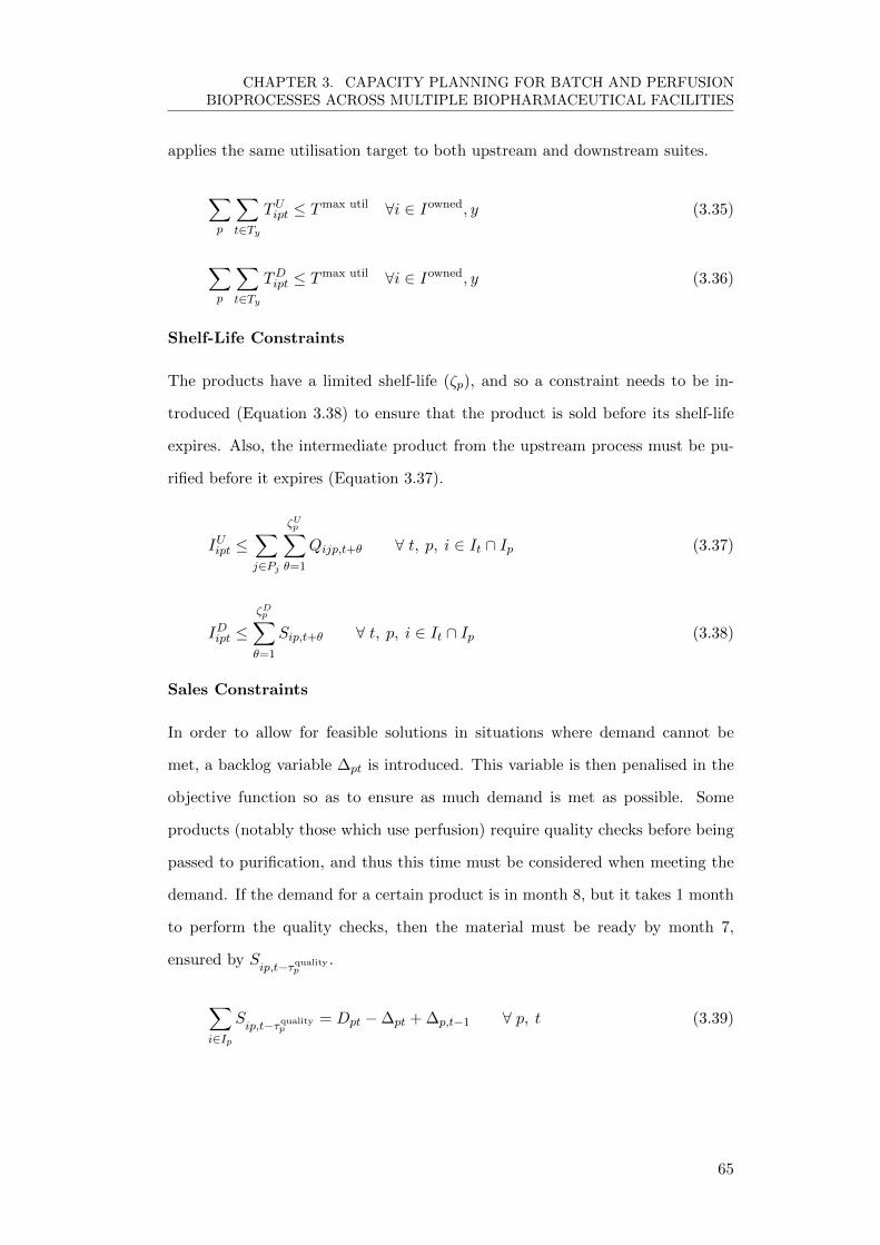
CHAPTER 3. CAPACITY PLANNING FOR BATCH AND PERFUSIONBIOPROCESSES ACROSS MULTIPLE BIOPHARMACEUTICAL FACILITIES
applies the same utilisation target to both upstream and downstream suites.
∑p
∑t∈Ty
TUipt ≤ Tmax util ∀i ∈ Iowned, y (3.35)
∑p
∑t∈Ty
TDipt ≤ Tmax util ∀i ∈ Iowned, y (3.36)
Shelf-Life Constraints
The products have a limited shelf-life (ζp), and so a constraint needs to be in-
troduced (Equation 3.38) to ensure that the product is sold before its shelf-life
expires. Also, the intermediate product from the upstream process must be pu-
rified before it expires (Equation 3.37).
IUipt ≤∑j∈Pj
ζUp∑θ=1
Qijp,t+θ ∀ t, p, i ∈ It ∩ Ip (3.37)
IDipt ≤ζDp∑θ=1
Sip,t+θ ∀ t, p, i ∈ It ∩ Ip (3.38)
Sales Constraints
In order to allow for feasible solutions in situations where demand cannot be
met, a backlog variable ∆pt is introduced. This variable is then penalised in the
objective function so as to ensure as much demand is met as possible. Some
products (notably those which use perfusion) require quality checks before being
passed to purification, and thus this time must be considered when meeting the
demand. If the demand for a certain product is in month 8, but it takes 1 month
to perform the quality checks, then the material must be ready by month 7,
ensured by Sip,t−τquality
p.
∑i∈Ip
Sip,t−τquality
p= Dpt −∆pt + ∆p,t−1 ∀ p, t (3.39)
65

CHAPTER 3. CAPACITY PLANNING FOR BATCH AND PERFUSIONBIOPROCESSES ACROSS MULTIPLE BIOPHARMACEUTICAL FACILITIES
3.3.2 Objective function
The discount factor is calculated as:
εt =
(1 + f
1 + g
)t−1
(3.40)
where f and g are the inflation and interest rate respectively.
The individual costs have been broken down as follows:
Inventory cost = IC =∑i
∑p
∑t
εt(ρip(I
Uipt+IDipt)+ρcarry
ip (IUipt+IDipt))
(3.41)
Inventory penalty cost = IPC =∑p
∑t
εt(Ipenaltyip (Iunder,U
ipt +Iunder,Dipt )
)(3.42)
Variable cost = V C =∑i
∑p
∑t
εt(ηbiasip (ηUipB
Uipt + ηDipB
Dipt))
(3.43)
Fixed cost = FC =∑
i∈Iowned
∑t
εt(ucost,Ui UUi + ucost,D
i UDi)
(3.44)
Transportation cost = TC =∑i
∑j
∑p
∑t
εt(qcijQijpt) (3.45)
Waste cost = WC =∑i
∑p
∑t
εt(wcostWipt
)(3.46)
Backlog penalty cost = BPC =∑p
∑t
εt(δp∆pt)
)(3.47)
Facility investment = FI =∑i
∑t
εt(κiKit
)(3.48)
Retrofitting cost = RC =∑i
∑p
∑t
εt(λUipL
Uipt + λDipL
Dipt
)(3.49)
Licence cost = LC =∑i
∑p
∑t
εt(λipL
Uipt
)(3.50)
The total cost consists of all the above costs summed together, and finally
equations 3.1-3.51 form the MILP problem to be optimised.
Minimise Total Cost = IC+IPC+V C+FC+TC+WC+BPC+FI+RC+LC
(3.51)
66
CHAPTER 3. CAPACITY PLANNING FOR BATCH AND PERFUSIONBIOPROCESSES ACROSS MULTIPLE BIOPHARMACEUTICAL FACILITIES
3.3.3 Optimisation Strategies
To obtain a good solution within reasonable time becomes increasingly more
difficult as the number of products, facilities or time periods being captured rises.
In order to achieve better solutions, a rolling time horizon was used, whereby a
smaller optimisation problem was run first, and part of the solution to this sub-
problem was used to initiate the subsequent larger problem. For example, if
the capacity plan was for 8 years, the first sub-problem could be a 4 year plan,
and once this has solved the second sub-problem could be 5 years in length,
but with the binary variables in the first year fixed to the solution from the
previous sub-problem. The next sub-problem would be 6 years in length, with
the first 2 years fixed from previous solutions, and the process continues until the
full 8 years has been captured. Although this approach is unlikely to find the
true optimum (since optimality gaps are accumulated for each sub-problem), for
the example investigated in this work it can provide better solutions than the full
scale optimisation under finite time. It should be stressed that given an unlimited
amount of time, the full scale mode will always provide the best solution. Figure
3.3 shows a rolling time horizon where only four years are actually optimised in
any given sub-problem, with the time horizon expanding by one year each time,
fixing the binary variables of earlier years using the solution from the previous
sub-problem. The rolling horizon approach implemented in this work avoids
infeasible situations by allowing backlogs to accumulate if demands in future years
are greater than the model was previously able to detect in the sub-problems.
Backlogs are penalised in the objective function, hence inferior solutions could
arise. However, in the base case presented here, the rolling time horizon approach
performed better than the full model in finite time.
67

CHAPTER 3. CAPACITY PLANNING FOR BATCH AND PERFUSIONBIOPROCESSES ACROSS MULTIPLE BIOPHARMACEUTICAL FACILITIES
Sub problem 1 2 3 4 5 6 7 8
1
2
3
4
5
Year
Figure 3.3: Illustration of a rolling time horizon. Dark grey boxes show yearswhere optimisation takes place, white boxes where no optimisation occurs, andlight grey boxes where the binary variables are fixed from the previous solution.
3.4 Illustrative Example
3.4.1 Input Data
This framework is tested on a case study of a generic portfolio of four drugs
and four facilities, key details of which are listed in Tables 3.1-3.4. Representa-
tive data for this case study were derived from literature sources (for example,
(Marichal-Gallardo and Alvarez, 2012)) as well as through discussions with indus-
trial practitioners involved in fed-batch and perfusion processes as well as produc-
tion planning. The four facilities consist of two in-house facilities, one contract
manufacturer, and one facility that can be built in the future if required. The
four products are in differing stages of clinical trials, but the demands modelled
here are for when the products reach the consumer market. Hence the points
where demands start in Table 3.3 differ according to how close the product is to
market penetration. The time horizon for this case study is eight years.
The quality control / quality assurance (QC/QA) time shown in Table 3.1 is
only applicable to perfusion processes, whereby the intermediate frozen material
from fermentation is checked prior to purification. This can lead to a substantial
lag between material being produced in the fermentation step and it being able
to be purified and thus meet demand, hence is included in the model.
Not all products can be manufactured in every facility, and for those combi-
nations which are allowed there may be a one-off retrofitting cost associated with
initial production. For example, for strategic reasons a company may wish to
keep the production of one of their products to in-house facilities only, and thus
68
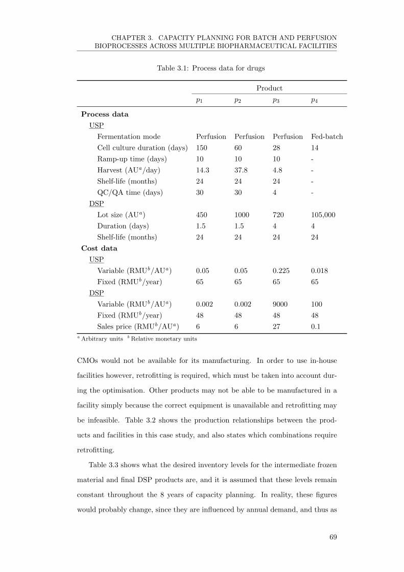
CHAPTER 3. CAPACITY PLANNING FOR BATCH AND PERFUSIONBIOPROCESSES ACROSS MULTIPLE BIOPHARMACEUTICAL FACILITIES
Table 3.1: Process data for drugs
Product
p1 p2 p3 p4
Process data
USP
Fermentation mode Perfusion Perfusion Perfusion Fed-batch
Cell culture duration (days) 150 60 28 14
Ramp-up time (days) 10 10 10 -
Harvest (AUa/day) 14.3 37.8 4.8 -
Shelf-life (months) 24 24 24 -
QC/QA time (days) 30 30 4 -
DSP
Lot size (AUa) 450 1000 720 105,000
Duration (days) 1.5 1.5 4 4
Shelf-life (months) 24 24 24 24
Cost data
USP
Variable (RMUb/AUa) 0.05 0.05 0.225 0.018
Fixed (RMUb/year) 65 65 65 65
DSP
Variable (RMUb/AUa) 0.002 0.002 9000 100
Fixed (RMUb/year) 48 48 48 48
Sales price (RMUb/AUa) 6 6 27 0.1a Arbitrary units b Relative monetary units
CMOs would not be available for its manufacturing. In order to use in-house
facilities however, retrofitting is required, which must be taken into account dur-
ing the optimisation. Other products may not be able to be manufactured in a
facility simply because the correct equipment is unavailable and retrofitting may
be infeasible. Table 3.2 shows the production relationships between the prod-
ucts and facilities in this case study, and also states which combinations require
retrofitting.
Table 3.3 shows what the desired inventory levels for the intermediate frozen
material and final DSP products are, and it is assumed that these levels remain
constant throughout the 8 years of capacity planning. In reality, these figures
would probably change, since they are influenced by annual demand, and thus as
69
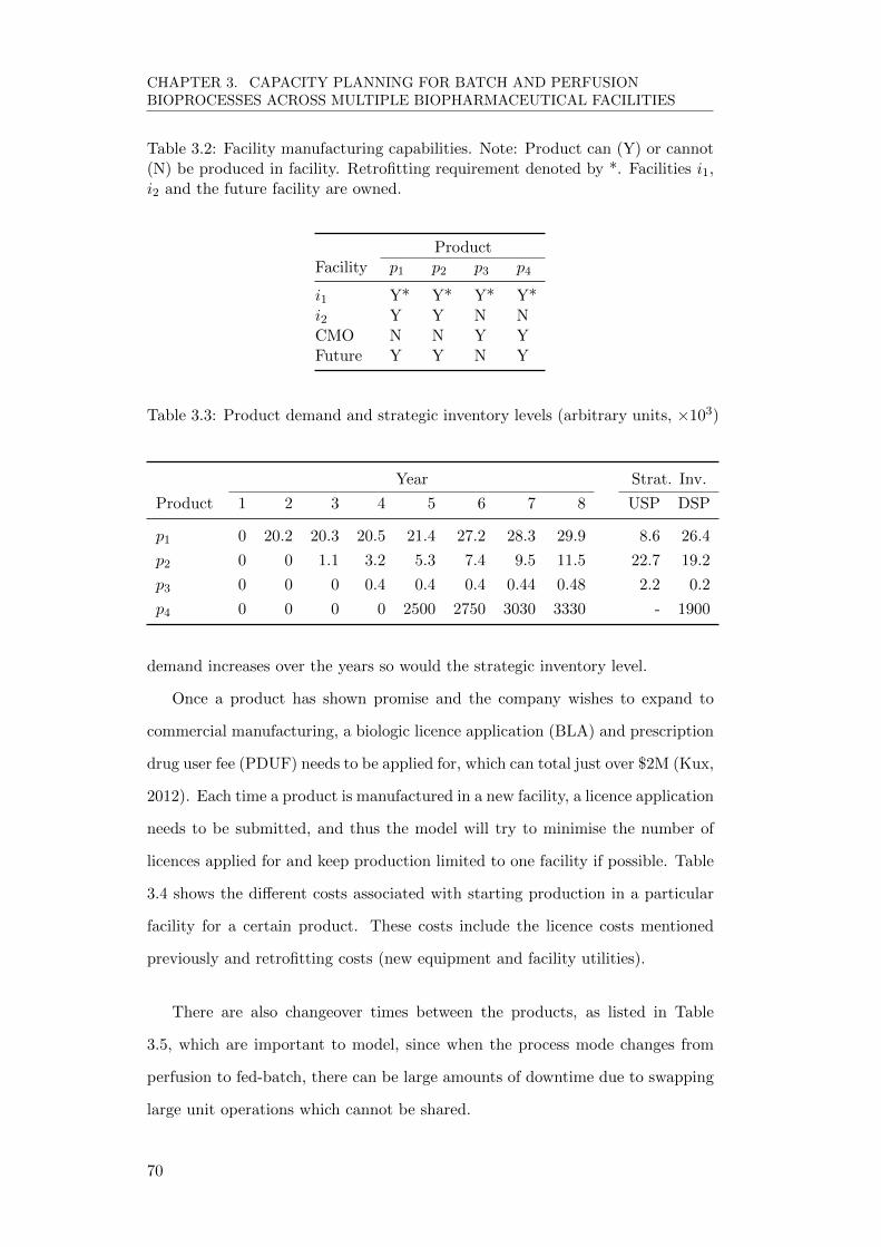
CHAPTER 3. CAPACITY PLANNING FOR BATCH AND PERFUSIONBIOPROCESSES ACROSS MULTIPLE BIOPHARMACEUTICAL FACILITIES
Table 3.2: Facility manufacturing capabilities. Note: Product can (Y) or cannot(N) be produced in facility. Retrofitting requirement denoted by *. Facilities i1,i2 and the future facility are owned.
ProductFacility p1 p2 p3 p4
i1 Y* Y* Y* Y*i2 Y Y N NCMO N N Y YFuture Y Y N Y
Table 3.3: Product demand and strategic inventory levels (arbitrary units, ×103)
Year Strat. Inv.
Product 1 2 3 4 5 6 7 8 USP DSP
p1 0 20.2 20.3 20.5 21.4 27.2 28.3 29.9 8.6 26.4
p2 0 0 1.1 3.2 5.3 7.4 9.5 11.5 22.7 19.2
p3 0 0 0 0.4 0.4 0.4 0.44 0.48 2.2 0.2
p4 0 0 0 0 2500 2750 3030 3330 - 1900
demand increases over the years so would the strategic inventory level.
Once a product has shown promise and the company wishes to expand to
commercial manufacturing, a biologic licence application (BLA) and prescription
drug user fee (PDUF) needs to be applied for, which can total just over $2M (Kux,
2012). Each time a product is manufactured in a new facility, a licence application
needs to be submitted, and thus the model will try to minimise the number of
licences applied for and keep production limited to one facility if possible. Table
3.4 shows the different costs associated with starting production in a particular
facility for a certain product. These costs include the licence costs mentioned
previously and retrofitting costs (new equipment and facility utilities).
There are also changeover times between the products, as listed in Table
3.5, which are important to model, since when the process mode changes from
perfusion to fed-batch, there can be large amounts of downtime due to swapping
large unit operations which cannot be shared.
70

CHAPTER 3. CAPACITY PLANNING FOR BATCH AND PERFUSIONBIOPROCESSES ACROSS MULTIPLE BIOPHARMACEUTICAL FACILITIES
Table 3.4: Initial start-up costs (including retrofitting, CMO negotiation fees,and licences) in relative monetary units.
Product
p1 p2 p3 p4
USP
i1 32.5 32.5 32.5 32.5
i2 0 0 - -
CMO - - 7 7
Future 10 10 - 10
DSP
i1 87.5 87.5 87.5 87.5
i2 0 0 - -
CMO - - 7 7
Future 10 10 - 10
Table 3.5: Changeover times between products. The units are in days, andrepresent the time taken to change from product p′ to p.
Product (p)
p1 p2 p3 p4
Product
(p′)
p1 7 7 7 14
p2 7 7 7 14
p3 7 7 7 14
p4 14 14 14 7
71

CHAPTER 3. CAPACITY PLANNING FOR BATCH AND PERFUSIONBIOPROCESSES ACROSS MULTIPLE BIOPHARMACEUTICAL FACILITIES
3.4.2 Computational Results
The model optimised the production plan of the four products across four avail-
able facilities. The results in Figure 3.4 show the plan over 8 years for different
demand scenarios. The base case requires the use of a CMO to meet the demand
for p3 and excess demand for p4. Note that the manufacturing of a product is
kept within one facility if possible so as to minimise licence fees. It is clear to see
that when the demand is low, all production can be met in-house and without
further expansion. Higher demands require almost full use of all the facilities
available, and expansion to a CMO and new facility. Despite not being shown
here, the market demands for all the products were met in full for almost all
scenarios (100% customer service level). Only in the last year of the +50% de-
mand case was there a small backlog for p3 and p4 (customer service level of
95%). Therefore, from a strategic viewpoint, the scenario with higher demand
looks less robust since the facilities are heavily utilised and there are already
small backlogs accumulating. There is very little margin for error should there
be a contamination or failed batches, thus extra capacity would be desirable.
A cost breakdown for the three demand cases shown in Figure 3.5 was con-
ducted and shows a clear increase in cost attributed to CMO activity in the
higher demand case (Figure 3.5c). For in-house production, the ratio between
variable to fixed costs ranges from approximately 1:7 (low demand) to 1:4 (high
demand). This range is justifiable, since as the demand increases, so too will the
variable costs, whilst the fixed costs will remain unchanged. It should be noted
that for this particular case study, once production in a facility has started, an-
nual fixed costs will be applied to that facility from that point onwards, because
most activities included in the fixed costs (such as labour, facility maintenance
and cleaning) will be on-going even if there is an idle year. The higher demand
case also shows that 5% of the total cost comes from the investment required to
build the new facility.
Capital expenditure information for all three demand cases is shown in Figure
3.6, and correlates to the retrofitting and facility investment costs in Figure 3.5.
72

CHAPTER 3. CAPACITY PLANNING FOR BATCH AND PERFUSIONBIOPROCESSES ACROSS MULTIPLE BIOPHARMACEUTICAL FACILITIES
(a)
(b)
(c)
Figure 3.4: Manufacturing schedule for (a) the base case , (b) -50% demand and(c) +50% demand.
The capital expenditures for the reduced demand case and base case are only
that of retrofitting. For the higher demand scenario a new facility is required,
and the cost of building the facility is spread out over four years, hence the
expenditure between years one to four. Retrofitting costs are minimised by the
model attempting to keep production within one facility if possible.
Another scenario that may occur is variability in titres for certain products.
Process parameters for products in early stages of development are not as well-
known as process parameters for commercial products or products in late stage
development. Also, when approaching a CMO they may have superior technolo-
73
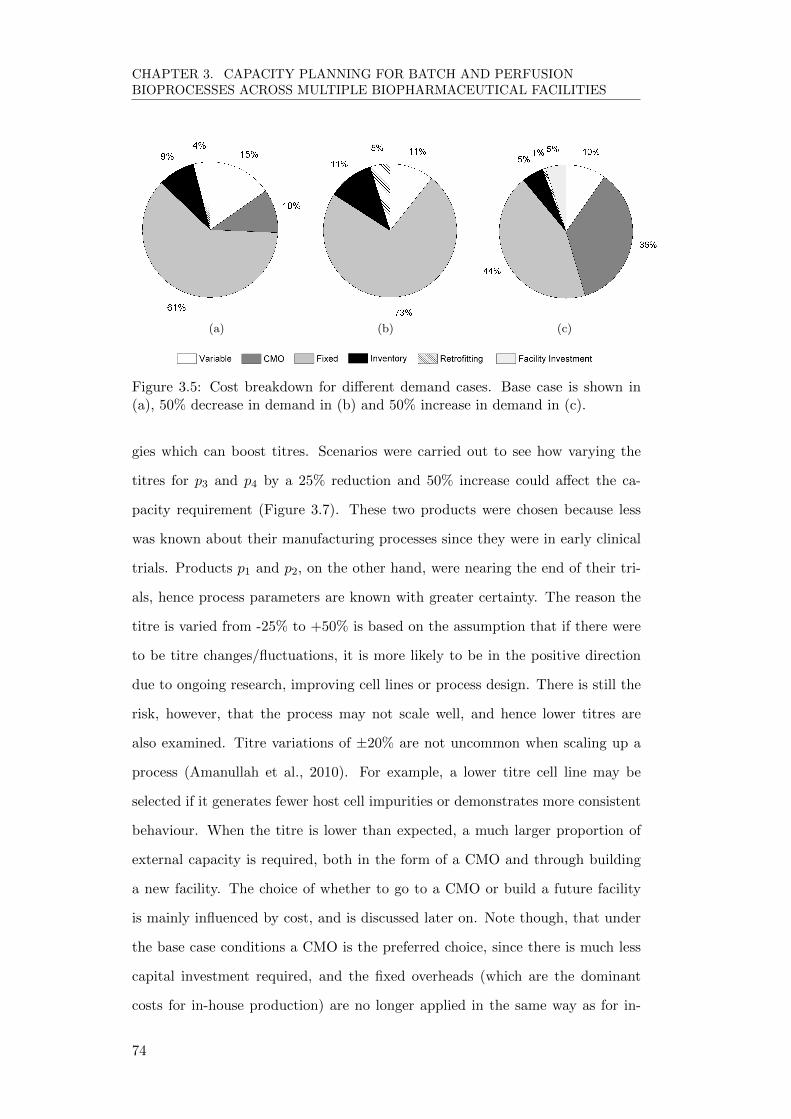
CHAPTER 3. CAPACITY PLANNING FOR BATCH AND PERFUSIONBIOPROCESSES ACROSS MULTIPLE BIOPHARMACEUTICAL FACILITIES
(a) (b) (c)
Figure 3.5: Cost breakdown for different demand cases. Base case is shown in(a), 50% decrease in demand in (b) and 50% increase in demand in (c).
gies which can boost titres. Scenarios were carried out to see how varying the
titres for p3 and p4 by a 25% reduction and 50% increase could affect the ca-
pacity requirement (Figure 3.7). These two products were chosen because less
was known about their manufacturing processes since they were in early clinical
trials. Products p1 and p2, on the other hand, were nearing the end of their tri-
als, hence process parameters are known with greater certainty. The reason the
titre is varied from -25% to +50% is based on the assumption that if there were
to be titre changes/fluctuations, it is more likely to be in the positive direction
due to ongoing research, improving cell lines or process design. There is still the
risk, however, that the process may not scale well, and hence lower titres are
also examined. Titre variations of ±20% are not uncommon when scaling up a
process (Amanullah et al., 2010). For example, a lower titre cell line may be
selected if it generates fewer host cell impurities or demonstrates more consistent
behaviour. When the titre is lower than expected, a much larger proportion of
external capacity is required, both in the form of a CMO and through building
a new facility. The choice of whether to go to a CMO or build a future facility
is mainly influenced by cost, and is discussed later on. Note though, that under
the base case conditions a CMO is the preferred choice, since there is much less
capital investment required, and the fixed overheads (which are the dominant
costs for in-house production) are no longer applied in the same way as for in-
74

CHAPTER 3. CAPACITY PLANNING FOR BATCH AND PERFUSIONBIOPROCESSES ACROSS MULTIPLE BIOPHARMACEUTICAL FACILITIES
1 2 3 4 5 6 7 80
20
40
60
80
100
Cap
ital E
xpe
nditu
re (
RM
U)
Year
Base Case50% Demand150% Demand
Figure 3.6: Capital expenditure profiles for the base case, 50% demand, and 150%demand.
house facilities. The CMO would still pass on its fixed costs to its customers, but
if manufacturing does not span an entire year and the CMO has other clients,
this will amount to less than would have otherwise been spent in-house. A CMO
alone would not have been enough to meet demand for the reduced titre scenario,
hence the future facility was required. With higher titres, the model pushes for
a greater proportion of in-house manufacturing (75%), since there is now unused
capacity in the existing facilities.
This case study includes a CMO in the list of available facilities, and as
such the costs of production there will be different to the in-house production
costs shown in Table 3.1. The cost of production in a CMO can be up to three
times greater than in-house manufacturing, depending on the scale of production
(Kelley, 2009). In the base case we have stated that the CMO costs are 50%
higher. However, this is only an assumption, and hence the model was used to
show what would happen to the capacity plan if the CMO costs were to change.
CMOs are naturally more expensive than in-house production, since they not
only need to cover their costs but also charge commission. The extra amount
that is paid will be dependent on the CMO’s experience, location and technology
it has to offer. Given that the CMO costs in this particular case study are
75

CHAPTER 3. CAPACITY PLANNING FOR BATCH AND PERFUSIONBIOPROCESSES ACROSS MULTIPLE BIOPHARMACEUTICAL FACILITIES
0
2000
2500
3000
Cos
t (R
MU
)
-30 -20 -10 0 10 20 30 40 50 600
25
50
75
100
Allo
catio
n of
tota
l ut
ilils
atio
n (%
)
Titre Change (%)
FutureCMOIn-house
Figure 3.7: Cost and utilisation vs. titre variance. The size of the bubblesrepresent the amount of extra capacity required to meet the demand. This extracapacity could be sourced from a CMO, or a future facility. The utilisationpercentage used for this figure relates to the USP only.
uncertain, an analysis was conducted to see how much more expensive the CMO
had to become before it became cheaper to build a new facility and produce
in-house. Figure 3.8 shows that once the CMO becomes 50% more expensive
than in-house production, a future facility provides alternative means of meeting
market demand at lower costs. The utilisation of the CMO decreases as the cost
of the CMO increases, but it never reaches 0% (even at 10 times the cost of
in-house production) because there is simply not enough capacity in the existing
facilities for the fermentation of p3 (which is being produced in the CMO). On
top of this, the future facility cannot produce p3, hence the fall in utilisation for
the CMO is not as large as one would initially expect.
Inventory profiles are useful to see whether the results are what one would
expect, since they clearly show whether the targets are being met and if there
is a lot of variation. Figure 3.9 shows the inventory profile for a perfusion-
mode process, and thus includes the upstream inventory level as well as the
downstream level. The figure also includes the strategic inventory levels that
should be maintained throughout the capacity plan. As noted before, the levels
may in reality change over time, but this model assumes them to remain constant.
76

CHAPTER 3. CAPACITY PLANNING FOR BATCH AND PERFUSIONBIOPROCESSES ACROSS MULTIPLE BIOPHARMACEUTICAL FACILITIES
1.0 1.5 2.0 2.5 3.00
10
20
30
40
50
60
70
80
90
100
Ave
rage
Util
isat
ion
(%)
Ratio of in-house:CMO cost, 1:x
CMOFuture
Figure 3.8: Utilisation of CMO facilities will decrease as its cost goes up, meaningmore production goes to in-house manufacturing. Since the existing in-housefacilities are already near full capacity in the base case, a future facility is builtin order to cope with demand. The utilisation percentages displayed here are forthe USP production and are the average monthly utilisation from the momentthe facility is used to the end of the eight year capacity plan.
The figure quickly demonstrates to a manager that the correct inventory levels
are being maintained in the middle of the plan, but near the end the levels tend to
drift downwards towards zero. This is actually owing to the fact that the penalty
applied for being under the strategic level in the objective function is applied
on a monthly basis, and thus near the end there are fewer months available to
penalise the shortfall, hence being under the strategic level no longer has such
a detrimental effect on the objective function. It therefore becomes cheaper to
have less product in storage.
Utilisation graphs can also be used to detect if extra capacity could be directed
towards an existing facility with low utilisation, or whether a facility is deemed to
be utilised too much and hence raises risk concerns should there be any unplanned
downtime. Figure 3.10 shows how facility i2 is almost at maximum capacity, with
only small breaks in production. The breaks in production are actually there on
purpose, since there is a utilisation cap of 75%. This provides leeway should
problems with failed batches occur. Facility i1 still has some available capacity,
but not enough to meet all demand, hence why the CMO is used in the base case.
77

CHAPTER 3. CAPACITY PLANNING FOR BATCH AND PERFUSIONBIOPROCESSES ACROSS MULTIPLE BIOPHARMACEUTICAL FACILITIES
20 40 60 800
500
1000
1500
2000
2500
3000
3500In
ven
tory
Le
vel (
arb
itra
ry u
nits
)
Month
USP InventoryDSP InventoryUSP Strategic TargetDSP Strategic Target
Figure 3.9: Inventory profile for p1, including both USP and DSP levels. Theoptimisation attempts to maintain strategic levels, but it will always place moreimportance on meeting demand first.
3.4.3 Computational Statistics
The optimisation was performed on an Intel Xeon W3565 Quad-core 3.2GHz
processor, with 6GB RAM running Microsoft Windows XP 64-bit. The frame-
work presented in this paper uses the CPLEX 12.5.1 solver (Corporation, 2012)
within GAMS 24.1.3 (Rosenthal, 2011) to solve the MILP problem, and outputs
the solution to Microsoft Excel for analysis using Visual Basic for Applications
(VBA). All optimisations (full-scale and rolling time horizon sub-problems) were
completed to within 5% optimality. The optimality gap is defined as:
Optimality gap =Best theoretical objective− Best feasibile objective
Best feasible objective
(3.52)
Here, the best theoretical objective is the solution obtained when the model
is relaxed and no longer has to abide by integer constraints. This is of course not
necessarily going to provide a feasible solution, but is a limit to how good the
solution could be if there were no integer constraints. The best feasible solution
78

CHAPTER 3. CAPACITY PLANNING FOR BATCH AND PERFUSIONBIOPROCESSES ACROSS MULTIPLE BIOPHARMACEUTICAL FACILITIES
(a) (b)
Figure 3.10: Monthly utilisation charts for in-house facilities (a) i1 (a) and (b)i2 for the base case. The percentages are of all products aggregated together forthe fermentation (USP). Note that i1 cannot be used for the first two years sinceduring that time another product (not modelled here) has been designated to it.
is one where integer constraints are in place. A 5% optimality gap means that the
objective value of the resulting solution is 5% away from the theoretical best if
there were no integer constraints. It may be the case that the solution is actually
the best solution available, but cannot be proven by the solver.
Although the case study outlined previously is relatively small, in that it only
consists of four products and four facilities (each with upstream and downstream
suites), the problem itself is computationally difficult to solve. Table 3.6 shows
how the number of variables and constraints in the model increases substantially
with increasing numbers of products, facilities and time periods. It should be
noted that these numbers would fluctuate depending on the individual case. For
example, if a product cannot be manufactured in a certain facility, then a set of
Table 3.6: Model statistics for various numbers of prod-ucts (p), facilities (i) and time periods (t). The casestudy presented in this paper is highlighted in bold.
Case Constraints Continuous
Variables
Discrete
Variables
2p, 2i, 48t 6,605 4,719 1,148
4p,4i,96t 33,183 25,037 5,184
8p, 8i, 192t 426,567 350,349 45,696
79
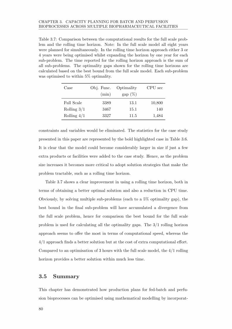
CHAPTER 3. CAPACITY PLANNING FOR BATCH AND PERFUSIONBIOPROCESSES ACROSS MULTIPLE BIOPHARMACEUTICAL FACILITIES
Table 3.7: Comparison between the computational results for the full scale prob-lem and the rolling time horizon. Note: In the full scale model all eight yearswere planned for simultaneously. In the rolling time horizon approach either 3 or4 years were being optimised whilst expanding the horizon by one year for eachsub-problem. The time reported for the rolling horizon approach is the sum ofall sub-problems. The optimality gaps shown for the rolling time horizons arecalculated based on the best bound from the full scale model. Each sub-problemwas optimised to within 5% optimality.
Case Obj. Func.
(min)
Optimality
gap (%)
CPU sec
Full Scale 3389 13.1 10,800
Rolling 3/1 3467 15.1 140
Rolling 4/1 3327 11.5 1,484
constraints and variables would be eliminated. The statistics for the case study
presented in this paper are represented by the bold highlighted case in Table 3.6.
It is clear that the model could become considerably larger in size if just a few
extra products or facilities were added to the case study. Hence, as the problem
size increases it becomes more critical to adopt solution strategies that make the
problem tractable, such as a rolling time horizon.
Table 3.7 shows a clear improvement in using a rolling time horizon, both in
terms of obtaining a better optimal solution and also a reduction in CPU time.
Obviously, by solving multiple sub-problems (each to a 5% optimality gap), the
best bound in the final sub-problem will have accumulated a divergence from
the full scale problem, hence for comparison the best bound for the full scale
problem is used for calculating all the optimality gaps. The 3/1 rolling horizon
approach seems to offer the most in terms of computational speed, whereas the
4/1 approach finds a better solution but at the cost of extra computational effort.
Compared to an optimisation of 3 hours with the full scale model, the 4/1 rolling
horizon provides a better solution within much less time.
3.5 Summary
This chapter has demonstrated how production plans for fed-batch and perfu-
sion bioprocesses can be optimised using mathematical modelling by incorporat-
80

CHAPTER 3. CAPACITY PLANNING FOR BATCH AND PERFUSIONBIOPROCESSES ACROSS MULTIPLE BIOPHARMACEUTICAL FACILITIES
ing various costs and time constraints, including sequence-dependent changeover
times. Both the upstream and downstream processes have been incorporated into
the model, and decoupled by the use of an intermediate storage step, which allows
greater flexibility for perfusion processes. The results demonstrate how capacity
plans can be quickly determined for various scenarios, aiding the manufacturer in
deciding when to consider outsourcing production, and the capital expenditure
likely to be required.
The solutions acquired using this framework were improved through a rolling
time horizon solution procedure, and the CPU time required was also substan-
tially reduced. Future work will include incorporating features to maintain strate-
gic inventory levels throughout the time horizon, addressing multiple objectives,
and reducing the optimality gap even further by appropriate model reformula-
tions.
81

CHAPTER 3. CAPACITY PLANNING FOR BATCH AND PERFUSIONBIOPROCESSES ACROSS MULTIPLE BIOPHARMACEUTICAL FACILITIES
3.6 Nomenclature
Indices
i, j facility (alias)p, p′ product (alias)t, θ time period (alias))y year
Sets
I faclitiesIp facilities which produce product pIt facilities available in time period tIowned owned facilitiesP productsP p perfusion productsPi products which are produced by facility iT time periodsTy time periods in year yY years
Scalars
H time horizon (days)R rejection coefficientτ retrofit retrofitting time)wcost waste cost
82
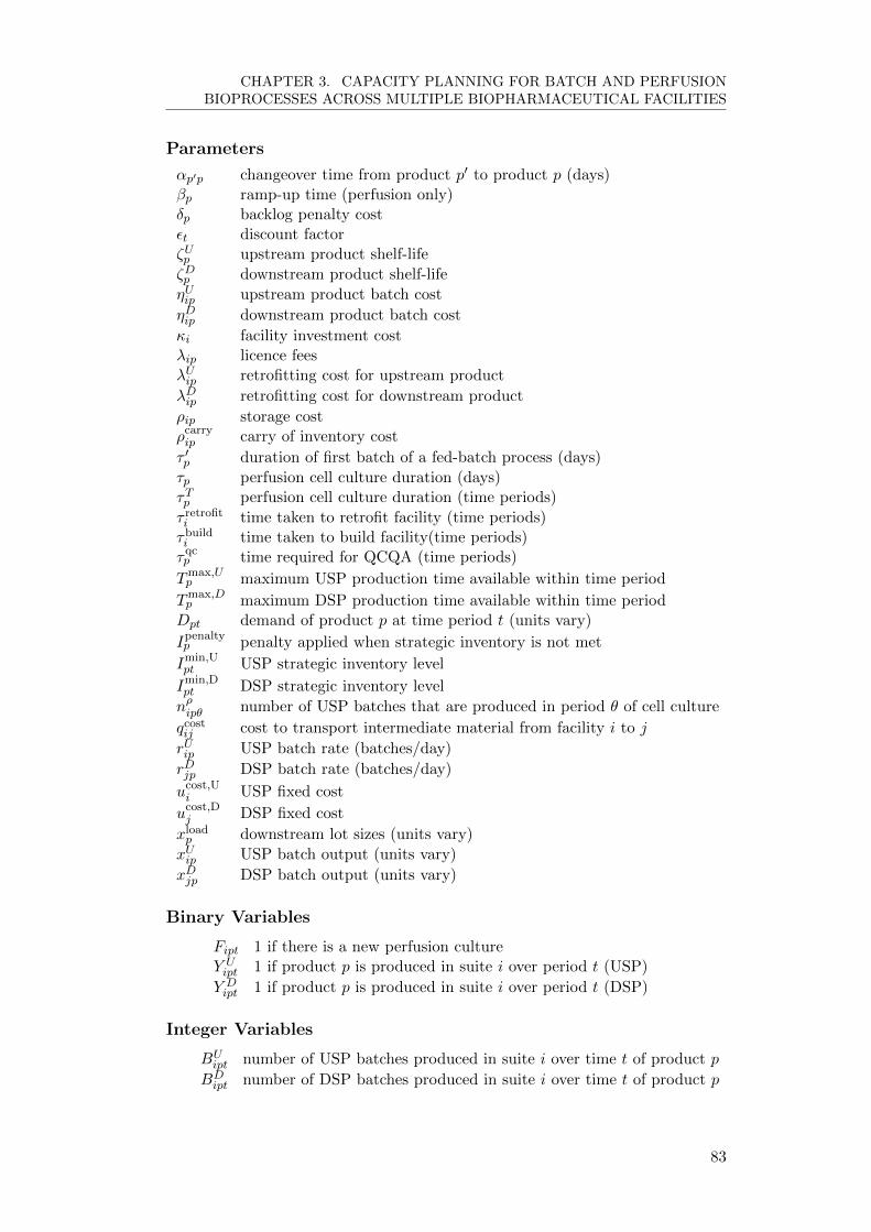
CHAPTER 3. CAPACITY PLANNING FOR BATCH AND PERFUSIONBIOPROCESSES ACROSS MULTIPLE BIOPHARMACEUTICAL FACILITIES
Parameters
αp′p changeover time from product p′ to product p (days)βp ramp-up time (perfusion only)δp backlog penalty costεt discount factorζUp upstream product shelf-life
ζDp downstream product shelf-life
ηUip upstream product batch cost
ηDip downstream product batch cost
κi facility investment costλip licence feesλUip retrofitting cost for upstream product
λDip retrofitting cost for downstream product
ρip storage costρcarryip carry of inventory cost
τ ′p duration of first batch of a fed-batch process (days)
τp perfusion cell culture duration (days)τTp perfusion cell culture duration (time periods)
τ retrofiti time taken to retrofit facility (time periods)τbuildi time taken to build facility(time periods)τqcp time required for QCQA (time periods)
Tmax,Up maximum USP production time available within time period
Tmax,Dp maximum DSP production time available within time periodDpt demand of product p at time period t (units vary)
Ipenaltyp penalty applied when strategic inventory is not met
Imin,Upt USP strategic inventory level
Imin,Dpt DSP strategic inventory level
nρipθ number of USP batches that are produced in period θ of cell culture
qcostij cost to transport intermediate material from facility i to j
rUip USP batch rate (batches/day)
rDjp DSP batch rate (batches/day)
ucost,Ui USP fixed cost
ucost,Dj DSP fixed cost
xloadp downstream lot sizes (units vary)
xUip USP batch output (units vary)
xDjp DSP batch output (units vary)
Binary Variables
Fipt 1 if there is a new perfusion cultureY Uipt 1 if product p is produced in suite i over period t (USP)
Y Dipt 1 if product p is produced in suite i over period t (DSP)
Integer Variables
BUipt number of USP batches produced in suite i over time t of product p
BDipt number of DSP batches produced in suite i over time t of product p
83

CHAPTER 3. CAPACITY PLANNING FOR BATCH AND PERFUSIONBIOPROCESSES ACROSS MULTIPLE BIOPHARMACEUTICAL FACILITIES
Positive Variables
AUipt, ADipt 1 if USP or DSP suite is available
Aretrofit,Uipt 1 if USP suite has been retrofitted
Aretrofit,Dipt 1 if DSP suite has been retrofitted
Afacilityit 1 if suite has been built
IUipt, IDipt USP/DSP inventory level
Iunder,Uipt USP inventory amount deviating from strategic level
Iunder,Dipt DSP inventory amount deviating from strategic level
Kit 1 if investment to construct facility i took place in period tLUipt 1 if retrofitting for product p in suite i starts at t
LDipt 1 if retrofitting for product p in suite i starts at t
Lipt, Ljpt 1 if licence payment for product p starts at t in suite iQijpt flow of material from USP to DSP suiteSjpt sales amount of product p (units vary)Wjpt amount of product p which is wasted (units vary)Y ′ipy 1 if new campaign starts
UUi , UDi 1 if there has been USP or DSP production in facility i
ZUip′pt, ZDip′pt 1 if there is a changeover from p′ → p in USP or DSP suites
∆pt demand not met
Free Variables
Cost manufacturing cost (to be minimised)
84

Chapter 4
Biopharmaceutical Capacity
Planning using a State Task
Network Topology
4.1 Introduction
In the previous chapter a standard MILP formulation was developed to address
the challenge of biopharmaceutical capacity planning involving batch and per-
fusion processes as well as build versus outsourcing production. Owing to the
computational complexity of the model, a rolling time horizon was required in
order to obtain solutions within reasonable time. This proved to be successful,
but one of the issues of using a rolling time horizon is that it is highly unlikely
that the overall optimal solution will be found, since at each sub-problem there is
an optimality gap. A method which could potentially solve the problem without
using a rolling time horizon would therefore be beneficial. This chapter explores
a more efficient mathematical formulation for the problem involving a state task
network representation. An alternative method using a genetic algorithm was also
developed, but was unfortunately not as successful. Details of that algorithm can
be found in Appendix A.
Resource task networks (RTNs) and state task networks (STNs) have been
85

CHAPTER 4. BIOPHARMACEUTICAL CAPACITY PLANNING USING A STATETASK NETWORK TOPOLOGY
described before in literature as a way of formulating a problem in a more generic
manner. Kondili et al. (1993) were the first to present the use of an STN as a
method of representing batch processes for short term scheduling problems. By
modelling the problem as an STN, ambiguities surrounding a process input and
output streams were removed. RTNs differ from STNs in the way a problem
is represented, namely the resources in RTNs show no distinction between raw
materials, equipment and utilities. The states in an STN represent material
states (for example, raw material, intermediate product, or final product). Using
an RTN or STN can simplify the modelling constraints, and thus help improve
performance.
The work presented in this chapter demonstrates how the standard mathe-
matical representation introduced in the previous chapter can be reformulated
using an STN topology, and how this contributes to performance improvements.
The model is then expanded to include additional features which help provide
more realistic manufacturing schedules. For example, retrofitting downtime is
now included whenever a suite is retrofitted for a new product. This makes it
less likely that a suite will be retrofitted for many products, since the downtime
would adversely affect capacity. Once an upstream suite has been retrofitted,
only products utilising the same process mode may be manufactured, unless an-
other retrofitting takes place. This more accurately represents real-life scenarios.
To add flexibility, only retrofitting downtime is applied to downstream suites.
CMO production has been altered to allow for the simultaneous manufacturing
of multiple products. This effectively means that the model can contain multi-
ple CMOs with little added computational effort. A constraint on the minimum
amount of material outsourced to a CMO in a given year has been added, to
more closely represent the nature of contract manufacturing. A feature of the
STN presented in this work is the ability to change time resolutions. In addition
to a rolling time horizon, a two month time resolution has been compared to
the one month resolution to determine whether improvements could be made in
performance and the solution.
An examination of the best way to expand in-house capacity through con-
86
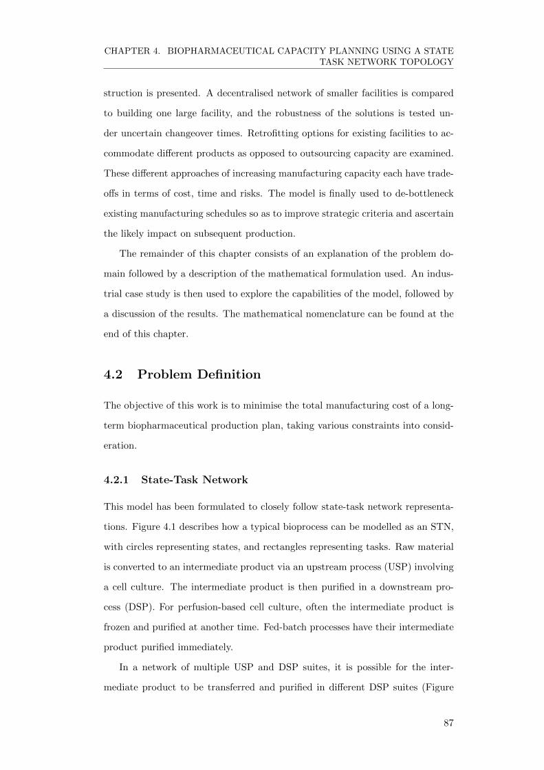
CHAPTER 4. BIOPHARMACEUTICAL CAPACITY PLANNING USING A STATETASK NETWORK TOPOLOGY
struction is presented. A decentralised network of smaller facilities is compared
to building one large facility, and the robustness of the solutions is tested un-
der uncertain changeover times. Retrofitting options for existing facilities to ac-
commodate different products as opposed to outsourcing capacity are examined.
These different approaches of increasing manufacturing capacity each have trade-
offs in terms of cost, time and risks. The model is finally used to de-bottleneck
existing manufacturing schedules so as to improve strategic criteria and ascertain
the likely impact on subsequent production.
The remainder of this chapter consists of an explanation of the problem do-
main followed by a description of the mathematical formulation used. An indus-
trial case study is then used to explore the capabilities of the model, followed by
a discussion of the results. The mathematical nomenclature can be found at the
end of this chapter.
4.2 Problem Definition
The objective of this work is to minimise the total manufacturing cost of a long-
term biopharmaceutical production plan, taking various constraints into consid-
eration.
4.2.1 State-Task Network
This model has been formulated to closely follow state-task network representa-
tions. Figure 4.1 describes how a typical bioprocess can be modelled as an STN,
with circles representing states, and rectangles representing tasks. Raw material
is converted to an intermediate product via an upstream process (USP) involving
a cell culture. The intermediate product is then purified in a downstream pro-
cess (DSP). For perfusion-based cell culture, often the intermediate product is
frozen and purified at another time. Fed-batch processes have their intermediate
product purified immediately.
In a network of multiple USP and DSP suites, it is possible for the inter-
mediate product to be transferred and purified in different DSP suites (Figure
87
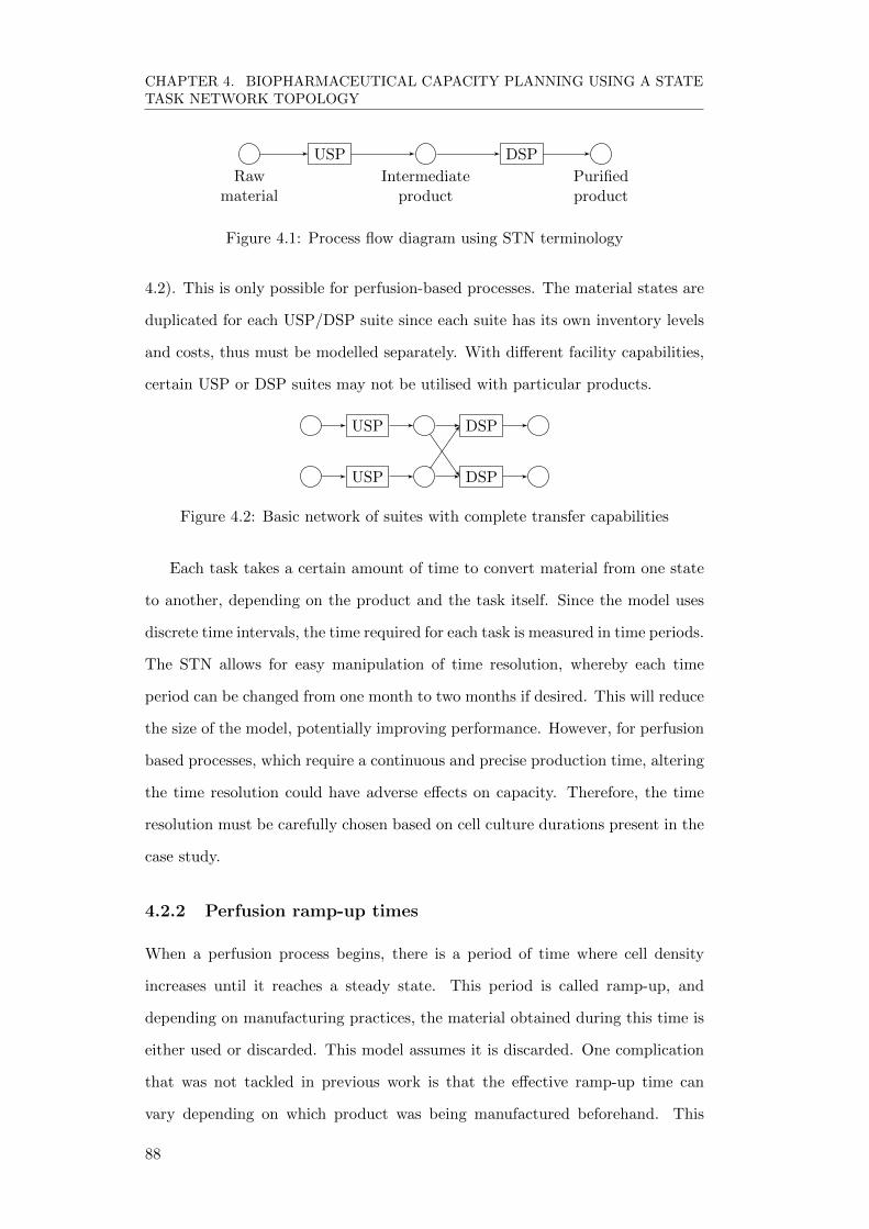
CHAPTER 4. BIOPHARMACEUTICAL CAPACITY PLANNING USING A STATETASK NETWORK TOPOLOGY
Rawmaterial
USP
Intermediateproduct
DSP
Purifiedproduct
Figure 4.1: Process flow diagram using STN terminology
4.2). This is only possible for perfusion-based processes. The material states are
duplicated for each USP/DSP suite since each suite has its own inventory levels
and costs, thus must be modelled separately. With different facility capabilities,
certain USP or DSP suites may not be utilised with particular products.
USP DSP
USP DSP
Figure 4.2: Basic network of suites with complete transfer capabilities
Each task takes a certain amount of time to convert material from one state
to another, depending on the product and the task itself. Since the model uses
discrete time intervals, the time required for each task is measured in time periods.
The STN allows for easy manipulation of time resolution, whereby each time
period can be changed from one month to two months if desired. This will reduce
the size of the model, potentially improving performance. However, for perfusion
based processes, which require a continuous and precise production time, altering
the time resolution could have adverse effects on capacity. Therefore, the time
resolution must be carefully chosen based on cell culture durations present in the
case study.
4.2.2 Perfusion ramp-up times
When a perfusion process begins, there is a period of time where cell density
increases until it reaches a steady state. This period is called ramp-up, and
depending on manufacturing practices, the material obtained during this time is
either used or discarded. This model assumes it is discarded. One complication
that was not tackled in previous work is that the effective ramp-up time can
vary depending on which product was being manufactured beforehand. This
88
CHAPTER 4. BIOPHARMACEUTICAL CAPACITY PLANNING USING A STATETASK NETWORK TOPOLOGY
characteristic only occurs if there are multiple bioreactors. When a new cell
culture begins from scratch, each bioreactor sequentially undergoes ramp-up, and
slowly all bioreactors will be online. However, if the same product was produced in
the previous campaign, then it is not necessary that all bioreactors must be offline.
Instead, a subset of the bioreactors undergo ramp-up at a time. In this way, the
effective time that was lost due to ramp-up is less. Since sequence-dependent
changeover variables are present in this model, it was possible to include this
feature.
4.2.3 Retrofitting considerations
Previous work addressed retrofitting from the perspective of capital expenditure,
but did not consider the implications of downtime associated with it. This model
expands the retrofitting constraints such that there is downtime applied to both
USP and DSP suites if they are retrofitted. To accomplish this, extra binary
variables needed to be introduced. Once retrofitted, depending on bioreactor size
and fittings within the suite, it may or may not be possible to continue produc-
tion of products using a different cell culture process. This added complexity
requires further constraints to be enforced. This model assumes it is possible to
switch products freely in DSP suites, but not in USP suites, owing to the size of
commercial bioreactors in fed-batch systems.
4.2.4 Contract manufacturing
The option to manufacture using a CMO is given more flexibility in this model,
by allowing multiple products to be produced simultaneously. Originally, if three
products were able to be manufactured in a CMO, they would have to be sched-
uled correctly with no overlap of production. Now, it would be possible for all
three products to be manufactured at the same time, effectively creating three
CMOs rather than one. There is still limited capacity in the CMO, but this
added flexibility means extra CMOs can be used without increasing the number
of variables or constraints in the model. A certain amount of time and money is
required to start licensing agreements with a CMO. In addition, CMOs generally
89

CHAPTER 4. BIOPHARMACEUTICAL CAPACITY PLANNING USING A STATETASK NETWORK TOPOLOGY
require a minimum amount to be manufactured at commercial scale. Thus to
ensure that this requirement is met, extra constraints are included to enforce
minimum annual production levels.
4.2.5 Decentralised production
The question of whether to build one large facility or multiple smaller facilities
is an important consideration when choosing how to expand capacity. Building
one large facility can reduce the overall capital expense, but offers less flexibil-
ity in terms of scheduling. Additionally, the fact that the facility is located in
one place can increase risk, since any unforeseen natural disasters could affect
manufacturing capabilities.
A network of smaller facilities can spread any natural or geopolitical risk, and
can also help minimise transportation costs to various markets across the world.
The flexibility in scheduling of having multiple facilities also helps production
teams find solutions when problems occur in one facility (for example, a contam-
ination breach). The trade-off is that the overall costs may be higher when total
fixed costs and capital expenditure are considered.
4.2.6 Multi-purpose facilities
Perfusion-mode cell cultures use vastly different bioreactor sizes than commer-
cial scale fed-batch cell cultures. This is due to the increased productivity that
perfusion processes allow, thereby reducing the required size of the bioreactors.
In contrast, most antibody production is carried out using larger stainless steel
bioreactors under fed-batch mode operation. Large stainless steel equipment is
difficult to move, and thus increases the logistical challenge of switching between
products. The dormant equipment must also be stored in a separate suite, which
may not always be feasible. Therefore, a challenge exists to make a facility truly
multi-purpose, whereby a production team can switch between different process
modes if required.
If a decision is made that prevents both types of processes from being manu-
factured in the same suite, then there will be ramifications on capacity planning.
90

CHAPTER 4. BIOPHARMACEUTICAL CAPACITY PLANNING USING A STATETASK NETWORK TOPOLOGY
Instead, it may be elected that retrofitting a facility will allow production for all
both types of process modes. This could be accomplished through careful plan-
ning and consideration of the retrofit, or through the use of alternative equipment
(for example, the use of disposables). Therefore, it is important to analyse the
requirements of a company based on their portfolio of products and facilities, to
determine whether various retrofitting options could help with capacity planning
and overall costs.
4.3 Mathematical Formulation
The following section describes the mathematics behind the model. The nomen-
clature can be found at the end of this chapter. Similar to the previous model,
many of the variables have been duplicated for the upstream and downstream
parts of the model (e.g., the number of batches produced). Therefore, the su-
perscripts U or D denote upstream or downstream, respectively. This model
continues to use a discrete time representation, with monthly time resolution (al-
though a two month resolution is also examined in the results section). With a
monthly resolution, an 8 year planning horizon would contain 96 time periods.
4.3.1 Technical and commercial constraints
Production Constraints
The number of upstream batches produced in time period t, for product p, in
fermentation suite i, is denoted by BUipt. Normally this could be calculated by
multiplying the production rate by the time used in a particular time period.
However, this requires extra time variables, and when taking into consideration
perfusion campaigns, can lead to less tight constraints. The approach taken
here utilises the idea of a state-task network (STN) to determine how many
batches are produced in a given time period, regardless of whether the product
is produced using a perfusion or fed-batch process, whilst still maintaining the
correct modelling conditions. Each perfusion cell culture will have a duration in
terms of time periods (τp). For each time period within a cell culture, a number
91

CHAPTER 4. BIOPHARMACEUTICAL CAPACITY PLANNING USING A STATETASK NETWORK TOPOLOGY
of batches are produced (nρipθ). The first part of Equation 4.1 sums over the
cell culture duration in reverse order to find out where the current time period
is within the cell culture, and then takes the number of batches from nρipθ. For
example, if a cell culture begins in month one (Fip,1 = 1), and lasts 5 months,
then if the number of batches for month 3 were to be calculated, the sum would
expand to: nρip,0Fip,3 + nρip,1Fip,2 + nρip,2Fip,1 = nρip,2 (where nρipθ is zero-indexed).
From this quantity, a number of batches (nUip′p) are subtracted due to changeovers
(ZUip′pt). This number that is subtracted will consider the downtime from cleaning
the facility and moving equipment, as well as ramp-up times. In the previous
model, ramp-up times were fixed per product, but in this model we allow greater
flexibility by linking it to the sequence-dependent changeover variables. Note
that the number of batches subtracted also depends on the facility being used,
since the batch rates may be different, thus for the same amount of downtime, a
greater or fewer number of batches will be subtracted.
BUipt =
τp−1∑θ=0
(nρipθFip,t−θ)−∑p′∈Pi
nUip′pZUip′pt ∀ p ∈ Pi ∩ P p ∩ P r, t, i ∈ It
(4.1)
For fed-batch processes, the idea is the same, except that since the cell cultures
are much shorter, rather than representing a single cell culture, Fipt represents
the fact that production is taking place in that time period. The value of nρipθ
is equal to the number of batches that can be produced in a time period, which
could consist of multiple fed-batch cell cultures. For example, if an E. coli cell
culture takes 5 days, then in a 30 day time period there could be a maximum of
6 batches (excluding downtime due to new campaigns and changeovers). Since
the USP and DSP production in fed-batch processes are coupled to one another,
there may be fewer than 6 batches if the downstream process is the bottleneck.
In this case, one would be able to predetermine the actual number of batches
that can be produced, and adjust nρipθ accordingly. Also, since the fed-batch
processes are not continuous (and thus do not need to run for the entire month),
92
CHAPTER 4. BIOPHARMACEUTICAL CAPACITY PLANNING USING A STATETASK NETWORK TOPOLOGY
the equality symbol has be changed to an inequality.
BUipt ≤
τp−1∑θ=0
(nρipθFip,t−θ)−∑p′∈Pi
nUip′pZUip′pt ∀ p ∈ {Pi − P p ∩ P r}, t, i ∈ It
(4.2)
To ensure that only one cell culture can take place in any suite at any given
time, Equation 4.3 is enforced. Not only does it prevent multiple products being
produced in the same time period, but it also back-checks up to the cell cul-
ture duration for each product, blocking any future production. This makes the
constraint more restrictive and helps fix the binary variable Fipt in more places.
∑p∈Pi
τp−1∑θ=0
Fip,t−θ ≤ 1 ∀ t, i ∈ It ∩ Iowned (4.3)
To prevent the case where cell cultures begin near the end of the time horizon and
there is not enough time for completion, the following constraint is introduced.
Fipt = 0 ∀ i, p, t ∈ T : t > (|T | − τp + 1) (4.4)
The calculation of downstream batches is similar to that of upstream, except
the concept of cell culture duration does not exist. Thus, if production takes
place in a time period (Y Dipt = 1), the number of batches is less than or equal
to the maximum number of DSP batches, nD,maxjpt , minus any subtracted due to
changeover downtime.
BDjpt ≤ n
D,maxjpt Y D
jpt−∑p′∈Pj
nDjp′pZDjp′pt ∀ t, p ∈ P r, j ∈ Jt∩Jp∩Jowned (4.5)
There may be a minimum number of DSP batches that are required per produc-
tion cycle. It should be noted that both nD,maxjpt and nD,min
jpt are parameters which
can vary with time, hence allowing flexibility should there be planned downtime
in one of the months, or if the maximum number of DSP batches changes due to
93

CHAPTER 4. BIOPHARMACEUTICAL CAPACITY PLANNING USING A STATETASK NETWORK TOPOLOGY
extra/fewer equipment.
BDjpt ≥ n
D,minjpt Y D
jpt ∀ t, p, j ∈ Jt ∩ Jp (4.6)
For fed-batch processes, where the USP and DSP production are coupled to each
other, the number of USP batches must equal the number of DSP batches, hence
the following constraints:
BDjpt = BU
ipt ∀ t, p ∈ {P r − P p}, j ∈ Jt ∩ Jp, i = j (4.7)
Y Djpt = Fipt ∀ t, p ∈ {P r − P p}, j ∈ Jt ∩ Jp, i = j (4.8)
The amount of material required per DSP batch, xloadp , must come from USP
inventory, and the flow of material from a USP to DSP suite is represented as
Qijpt. This only applies to perfusion-based products.
xloadp BD
jpt =∑
i∈Ip∩It
Qijpt ∀ t, p ∈ P r ∩ P p, j ∈ Jt ∩ Jp (4.9)
To prevent more that one product being produced simultaneously in the same
suite, the following constraint is included:
∑p∈Pj∩P r
Y Djpt ≤ 1 ∀ t, j ∈ Jt ∩ Jowned (4.10)
Timing Constraints
Changeovers occur when there is a product switch within the same suite. The
following equations enforce a changeover from product p′ → p if p′ was produced
in the previous time period. Changeovers for upstream production need to be
strict, because otherwise the model may choose to reduce the upstream produc-
tion time by arbitrarily adding a changeover that should not exist. For perfusion
processes, this can add inaccuracies to the modelling. If there is an idle period,
this model will assume that the changeover will take place in the idle period
and thus will not subtract from available production time. This is accomplished
94

CHAPTER 4. BIOPHARMACEUTICAL CAPACITY PLANNING USING A STATETASK NETWORK TOPOLOGY
by adjusting nδjp′p accordingly. These changeover constraints are different to the
ones used in the previous chapter, since they sum over one set of the products,
thereby reducing the number of constraints. A pseudo-product is introduced to
allow for idle periods, all real products are members of P r. For distinct p′ and p:
∑p∈Pi
ZUip′pt = Fip′,t−τp′ ∀ p′, t > τp′ , i ∈ Ip′ ∩ It ∩ Iowned (4.11)
∑p′∈Pi
ZUip′pt = Fipt ∀ t, p, i ∈ Ip ∩ It ∩ Iowned (4.12)
ZUip′pt = Fipt ∀ p′ /∈ P r, p, i ∈ Ip ∩ It ∩ Iowned, t = τ starti (4.13)
Since changeovers are less strict for downstream production (owing to there
not being any continuous downstream processes being modelled here), only one
equation is necessary. By using the older version of the changeover constraint,
the pseudo-product for downstream variables is not required, thereby reducing
the number of additional discrete variables. The impact of the extra discrete
variables would not warrant the reduction in the number of constraints.
ZDjp′pt ≥ Y Djpt + Y D
jp′,t−1 − 1 ∀ t, p′ ∈ P r, p ∈ P r, j ∈ Jp′ ∩ Jt ∩ Jp (4.14)
Availability Constraints
To prevent cases where production takes place in a suite which is not yet ready,
the following constraints are included. AUipt is equal to 1 if the suite is ready for
production, and this is linked to whether the facility has been built (Ait) and/or
retrofitted (Aretrofit,Uipt ). These variables are in turn linked to the investment con-
straints which follow this section.
Fipt ≤ AUipt ∀ t, i ∈ It, p ∈ Pi ∩ P r (4.15)
Y Djpt ≤ ADjpt ∀ t, j ∈ Jt, p ∈ Pj ∩ P r (4.16)
95

CHAPTER 4. BIOPHARMACEUTICAL CAPACITY PLANNING USING A STATETASK NETWORK TOPOLOGY
AUipt ≤ Ait ∀ t, i ∈ It, p ∈ Pi ∩ P r (4.17)
AUipt ≤ Aretrofit,Uipt ∀ t, i ∈ It, p ∈ Pi ∩ P r (4.18)
ADjpt ≤ Ajt ∀ t, j ∈ Jt, p ∈ Pj ∩ P r (4.19)
ADjpt ≤ Aretrofit,Djpt ∀ t, j ∈ Jt, p ∈ Pj ∩ P r (4.20)
Investment Constraints
In order to use a facility, it must first be built if it does not already exist. The
following equation forces Kit to 1 if that facility is to be used. This pseudo-binary
variable is then penalised in the objective function by a parameter representing
the construction cost. The constraint also ensures that the facility is not available
until after the construction time, τbuildi .
Ait ≤ Ai,t−1 +Ki,t−τbuildi
∀ i, t > τbuildi (4.21)
Licence costs are also considered, and they are modelled such that the licence is
per facility, rather than any individual suite.
AUipt ≤ AUip,t−1 + Lipt ∀ p ∈ P r, i ∈ Ip, t ∈ Ti (4.22)
ADjpt ≤ ADjp,t−1 + Ljpt ∀ p ∈ P r, j ∈ Jp, t ∈ Tj (4.23)
Similar to the investment constraints in the previous chapter, these equations
ensure that in order for a product to be manufactured in a facility, any relevant
retrofitting must be carried out. For example, LUipt is equal to 1 if retrofitting for
product p starts at time t in facility i. The investment for retrofitting must be
96

CHAPTER 4. BIOPHARMACEUTICAL CAPACITY PLANNING USING A STATETASK NETWORK TOPOLOGY
spent τ retrofiti time periods before the facility becomes available for that product.
Aretrofit,Uipt ≤ Aretrofit,U
ip,t−1 + LUip,t−τ retrofit
i∀ p ∈ P r, i ∈ Ip, t > τ retrofit
i (4.24)
Aretrofit,Djpt ≤ Aretrofit,D
jp,t−1 +LDjp,t−τ retrofit
j∀ p ∈ P r, j ∈ Jp, t > τ retrofit
j (4.25)
Retrofitting Constraints
One of the new features of this model is that of applying downtime when retrofitting
takes place. When a facility is being retrofitted for another product, current pro-
duction must stop. For these constraints to work, LUipt and LDjpt must be made
binary variables. The following equation forces there to be idle time in all time
periods where retrofitting is taking place. Idle time occurs when Fipt = 1 for the
pseudo-product, p /∈ P r.
τ retrofiti −1∑θ=0
Fip,t+θ ≥ τ retrofiti
∑p′∈P r∩Pi
LUip′t ∀ p /∈ P r, i ∈ Iretrofit, t ∈ Ti (4.26)
A similar concept applies to retrofitting downstream production, except that
the constraint here does not force idle time directly, but rather prevents other
products from being manufactured. The reason for this is that, as mentioned
in the downstream changeover constraints, there is no pseudo-product in down-
stream production. Without the pseudo-product, idle time cannot be directly
enforced.
τ retrofitj −1∑θ=0
Y Djp,t+θ ≤ τ retrofit
j (1−∑
p′∈P r∩Pj
LDjp′t) ∀ p ∈ P r, j ∈ J retrofit, t ∈ Tj
(4.27)
An upstream or downstream suite can only be retrofitted one product at a
time, hence the following constraints ensure that this requirement is met for both
97

CHAPTER 4. BIOPHARMACEUTICAL CAPACITY PLANNING USING A STATETASK NETWORK TOPOLOGY
USP and DSP suites.
∑p∈P r∩Pi
τ retrofiti −1∑θ=0
LUip,t+θ ≤ 1 ∀ i, t ∈ Ti (4.28)
∑p∈P r∩Pj
τ retrofitj −1∑θ=0
LDjp,t+θ ≤ 1 ∀ j, t ∈ Tj (4.29)
In the case of upstream suites, large equipment cannot be easily moved in
and out, especially if they are fixed. In this model, it is assumed that if a USP
suite has been retrofitted for a fed-batch product, then the perfusion processes
can no longer take place, unless the suite is retrofitted again, thereby preventing
fed-batch production. This limitation is only applied to USP suites, since it is
assumed that the DSP suite is more flexible due to the nature of the equipment
sizes.
∑p′∈P r∩Pp
Aretrofit,Uip′t ≤ 1−LUipt ∀ p ∈ {P r−P p}, i ∈ Iretrofit, t ∈ Ti∩Tp (4.30)
∑p′∈{P r−Pp}
Aretrofit,Uip′t ≤ 1−LUipt ∀ p ∈ P r∩P p, i ∈ Iretrofit, t ∈ Ti∩Tp (4.31)
CMO Constraints
This model places restrictions on the minimum amount of material that is pro-
duced in a CMO in a given year. This is to prevent the case where a CMO is
used sparingly just to meet the demand on the infrequent occasion where in-house
capacity is limited. It is more likely that, should a CMO be selected, there would
be a minimum amount produced during that campaign. The following equation
calculates how much material of a product was manufactured in a CMO that
98

CHAPTER 4. BIOPHARMACEUTICAL CAPACITY PLANNING USING A STATETASK NETWORK TOPOLOGY
year, Cjpy.
Cjpy =∑
t∈Ty∩Tj
xDjpBDjpt ∀ p ∈ P r, j ∈ {Jp − Jowned}, y (4.32)
If a CMO has been used in that year (Xjpy), then the minimum amount must
be enforced:
Cjpy ≥ xmin,CMOpy Xjpy ∀ p ∈ P r, j ∈ {Jp − Jowned}, y (4.33)
The following equation forces Xjpy to be equal to 1 when production of p has
occurred in that year.
∑y∈Yt
Xjpy ≥ Y Djpy ∀ p ∈ P r, j ∈ {Jp − Jowned}, t ∈ Tj (4.34)
Utilisation Constraints
There are maximum utilization targets for in-house facilities, and thus constraints
need to be put into place to accomplish this. For every in-house facility and each
year, the following equations restrict the total time used for each product in each
month of the year to be below the maximum allowed. Therefore, if the maximum
desired facility utilization is 75%, Havailable,y can be set to 270 days. The model
applies the same utilization target to both upstream and downstream suites. It
should be noted that these constraints limit actual production time, rather than
utilisation time. Therefore it does not include changeover or ramp-up times.
These could be included if desired, or Havailable,y could be adjusted to reflect this
difference.
∑p∈Pi∩P r
∑t∈Ty∩Ti
BUipt
rUip≤ Havailable,y ∀i ∈ Iowned, y (4.35)
99

CHAPTER 4. BIOPHARMACEUTICAL CAPACITY PLANNING USING A STATETASK NETWORK TOPOLOGY
∑p∈Pj∩P r
∑t∈Ty∩Tj
BDjpt
rDjp≤ Havailable,y ∀j ∈ Jowned, y (4.36)
The following two equations are shown if actual utilisation calculations are
required. They were used instead of the two equations above when comparing to
the previous chapter’s model.
∑p∈Pi∩P r
∑t∈Ty∩Ti
(BUipt +
∑p′∈Ip∩P r
αUip′pZUip′pt)/r
Uip ≤ Havailable,y ∀i ∈ Iowned, y
∑p∈Pj∩P r
∑t∈Ty∩Tj
(BDjpt +
∑p′∈Jp∩P r
αDjp′pZDjp′pt)/r
Djp ≤ Havailable,y ∀j ∈ Jowned, y
Fixed Cost Constraints
The modelling of fixed costs is the same here as it was in the previous chapter.
Upstream and downstream suite use (UUi and UDj ) is separated so that fixed costs
can be attributed individually. These constraints check to see whether the suite
has been used, and if so set UUi or UDj to 1. These variables are then used in the
objective function when applying fixed costs. If a suite has never been used over
the planning horizon (e.g., if it had never been built, or if no product was ever
allocated to it), then no fixed costs need to be applied for that suite. Also note
that only the facilities which are owned (Iowned) need to be subjected to fixed
costs.
UUi ≥ Fipt ∀ i ∈ Iowned, p ∈ Pi ∩ P r, t ∈ Ti (4.37)
UDj ≥ Yjpt ∀ j ∈ Iowned, p ∈ Pj ∩ P r, t ∈ Tj (4.38)
100
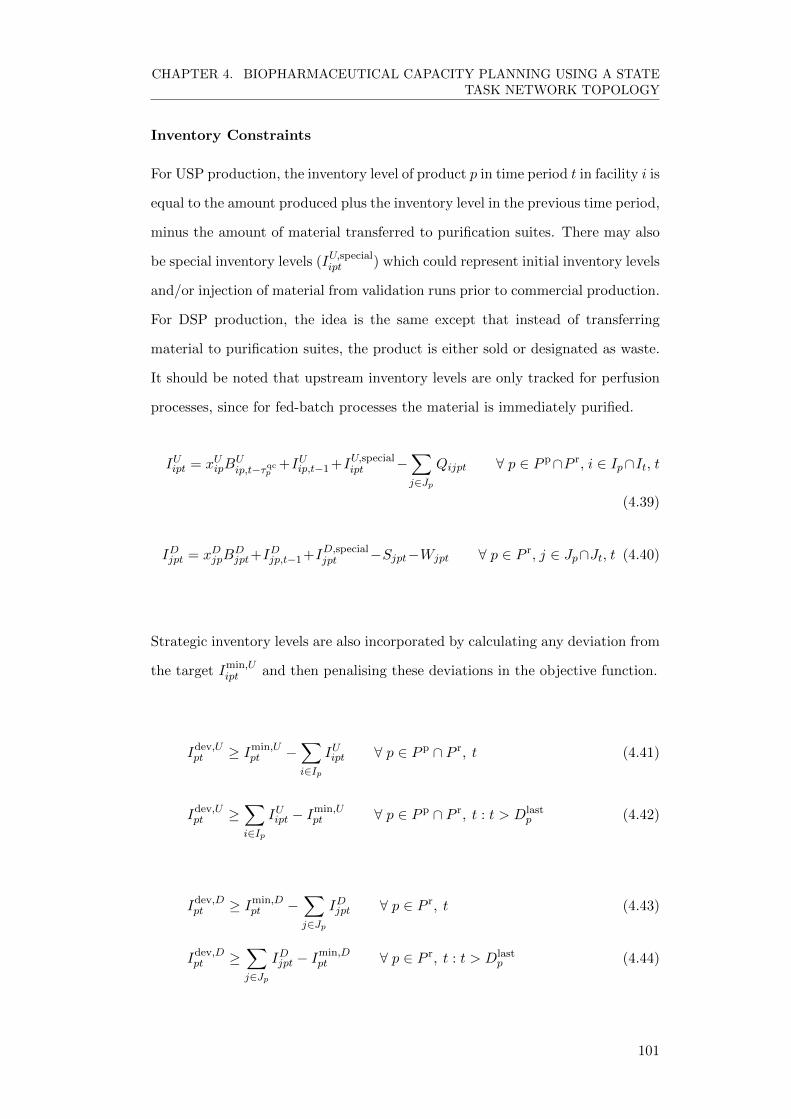
CHAPTER 4. BIOPHARMACEUTICAL CAPACITY PLANNING USING A STATETASK NETWORK TOPOLOGY
Inventory Constraints
For USP production, the inventory level of product p in time period t in facility i is
equal to the amount produced plus the inventory level in the previous time period,
minus the amount of material transferred to purification suites. There may also
be special inventory levels (IU,specialipt ) which could represent initial inventory levels
and/or injection of material from validation runs prior to commercial production.
For DSP production, the idea is the same except that instead of transferring
material to purification suites, the product is either sold or designated as waste.
It should be noted that upstream inventory levels are only tracked for perfusion
processes, since for fed-batch processes the material is immediately purified.
IUipt = xUipBUip,t−τqc
p+IUip,t−1 +IU,special
ipt −∑j∈Jp
Qijpt ∀ p ∈ P p∩P r, i ∈ Ip∩It, t
(4.39)
IDjpt = xDjpBDjpt+I
Djp,t−1+ID,special
jpt −Sjpt−Wjpt ∀ p ∈ P r, j ∈ Jp∩Jt, t (4.40)
Strategic inventory levels are also incorporated by calculating any deviation from
the target Imin,Uipt and then penalising these deviations in the objective function.
Idev,Upt ≥ Imin,U
pt −∑i∈Ip
IUipt ∀ p ∈ P p ∩ P r, t (4.41)
Idev,Upt ≥
∑i∈Ip
IUipt − Imin,Upt ∀ p ∈ P p ∩ P r, t : t > Dlast
p (4.42)
Idev,Dpt ≥ Imin,D
pt −∑j∈Jp
IDjpt ∀ p ∈ P r, t (4.43)
Idev,Dpt ≥
∑j∈Jp
IDjpt − Imin,Dpt ∀ p ∈ P r, t : t > Dlast
p (4.44)
101

CHAPTER 4. BIOPHARMACEUTICAL CAPACITY PLANNING USING A STATETASK NETWORK TOPOLOGY
Shelf-Life Constraints
The products have a limited shelf-life, and a constraint needs to be put in place
to ensure that the product is sold before its lifetime expires, or else it should be
discarded as waste. There is also a shelf-life for the intermediate product coming
from upstream production. In this case, the product must be purified before it
expires.
IUipt ≤∑j∈Pj
t+ζUp∑θ=t+1
Qijpθ ∀ i, p ∈ Pi ∩ P r, t ∈ Ti : t < (|T | − ζUp ) (4.45)
IDjpt ≤t+ζDp∑θ=t+1
Sjpθ ∀ j, p ∈ Pj ∩ P r, t ∈ Tj : t < (|T | − ζDp ) (4.46)
Sales Constraints
The amount sold is equal to the demand minus any backlogs. Since the backlogs
can accumulate, the amount that was late in the previous time period is also
considered, such that the model can make up for lost sales.
∑j∈Jp∩Jt
Sjpt = Dpt −∆pt + ∆p,t−1 ∀ p, t (4.47)
4.3.2 Objective function
The discount factor is calculated as:
εt =
(1 + f
1 + g
)t−1
(4.48)
where f and g are the inflation and interest rate respectively.
The individual costs have been broken down as follows:
Inventory cost = IC =∑i
∑p
∑t
εt(ρip(I
Uipt+IDipt)+ρcarry
ip (IUipt+IDipt))
(4.49)
102

CHAPTER 4. BIOPHARMACEUTICAL CAPACITY PLANNING USING A STATETASK NETWORK TOPOLOGY
Inventory penalty cost = IPC =∑p
∑t
εt(Ipenaltyip (Idev,U
ipt + Idev,Dipt )
)(4.50)
Variable cost = V C =∑i
∑p
∑t
εt(ηbiasip (ηUipB
Uipt + ηDipB
Dipt))
(4.51)
Fixed cost = FC =∑i
∑t∈Ti
εt(ucost,Ui UUi + ucost,D
i UDi)
(4.52)
Transportation cost = TC =∑i
∑j
∑p
∑t
εt(qcijQijpt) (4.53)
Waste cost = WC =∑i
∑p
∑t
εt(wcostWipt
)(4.54)
Backlog penalty cost = BPC =∑p
∑t
εt(δp∆pt)
)(4.55)
Facility investment = FI =∑i
∑t
εt(κiKit
)(4.56)
Retrofitting cost = RC =∑i
∑p
∑t
εt(λUipL
Uipt + λDipL
Dipt
)(4.57)
Licence cost = LC =∑i
∑p
∑t
εt(λipL
Uipt
)(4.58)
Minimise Total Cost = IC+IPC+V C+FC+TC+WC+BPC+FI+RC+LC
(4.59)
This chapter compares the STN to the standard representation (SR) described
in the previous chapter. To make a fair comparison, not all the constraints listed
above were used as described. The CMO features were excluded, as were the
constraints under the retrofitting subheading. Inventory level calculations did not
include special inventory levels, and inventory levels above strategic targets were
not considered. Changeover times were included in the utilisation calculations.
Equations 1 - 4.59 form the STN* model, and represent the STN with new
features.
103

CHAPTER 4. BIOPHARMACEUTICAL CAPACITY PLANNING USING A STATETASK NETWORK TOPOLOGY
Table 4.1: Process Data for Drugs in Case Study 2
Product
p1 p2 p3 p4 p5 p6
Product typeBlood-
factor
Blood-
factor
Blood-
factormAb Fab ADC
Process data
USP
Fermentation mode Perfa Perfa Perfa FBb FBb FBb
Cell culture duration (days) 150 120 60 10 3 10
Harvest (AUc/day) 120 130 490 - - -
QC/QA time (days) 60 30 30 - - -
DSP
Lot size (AUc) 320 450 1000 6 2 6
Duration (days) 1.5 1.5 1.5 1.5 3.5 3.5
Cost data
USP
Variable (RMUd/AUc) 0.005 0.005 0.005 0.004 0.007 0.004
Fixed (RMUd/year) 65 65 65 3.5 6.6 3.5
DSP
Variable (RMUd/AUc) 0.002 0.002 0.002 0.02 0.02 0.1
Fixed (RMUd/year) 48 48 48 5 15 5
CMO (RMUd/AUc) - - - 0.23 0.56 1a Perfusion b Fed-batch c Arbitrary units d Relative monetary units
4.4 Illustrative Example
In order to compare the STN to the standard mathematical model, optimisations
were run for two different case studies. The first case study is the same one as pre-
sented in the previous chapter, consisting of four products and four facilities. The
second case study consists of 6 products and 11 facilities. The second case study
was chosen to be larger than the first case study, so that we could examine the
performance of the mathematical model when presented with a larger portfolio
of products and facilities. Product information regarding process data and costs
are shown in Table 4.1. The six products are a mixture of perfusion mode cell
cultures and fed-batch cell cultures, reflecting the different product types being
manufactured (namely blood-factors and antibodies respectively). The fragment
104

CHAPTER 4. BIOPHARMACEUTICAL CAPACITY PLANNING USING A STATETASK NETWORK TOPOLOGY
Table 4.2: Product and facility capability matrix for Case Study 2. Note: B -both upstream and downstream capability, U - upstream only, N - no capability,* - retrofitting required.
Startingyear
Product USP scaleFacility p1 p2 p3 p4 p5 p6 p1 − p3 p4 − p6
i1 1 B B* B* B* B* B* 6 x 200 L 2 x 2000 Li2 1 U B B N N N 6 x 200 L 2 x 2000 Li3 1 U N N N N N 2 x 200 L -i4 5 N U U N N N 6 x 200 L -i5 7 N B B N N N 6 x 200 L -i6 3 N N N B B B - 2 x 2000 Li7 5 N N N B B B - 6 x 2000 Li8 6 N N N B B B - 2 x 2000 Li9 7 N N N B B B - 2 x 2000 Li10 8 N N N B B B - 2 x 2000 Li11 1 N N N B B B - 2 x 2000 L
Table 4.3: Costs for retrofitting, licences, and otherstart-up costs for Case Study 2 (relative monetaryunits)
Product
p1 p2 p3 p4 − p6
Licence /
start-up
cost
i1 5 5 5 5
i2 − i3 0 0 0 -
i4 - 5 5 -
i5 - 5 5 -
i6 − i10 - - - 5
i11 - - - 7
USP retrofit i1 0 16.5 16.5 11
DSP retrofit i1 0 38.5 38.5 44
105

CHAPTER 4. BIOPHARMACEUTICAL CAPACITY PLANNING USING A STATETASK NETWORK TOPOLOGY
antigen binding (Fab) product uses E. coli as the cell culture expression system,
and thus has a much shorter cell culture duration than mammalian cell alter-
natives. The downstream processing takes longer however, since extra steps are
required for pegylation and further polishing.
Table 4.4: Demand and strategic inventory profiles for Case Study 2(arbitrary units, ×102)
Year
Product 1 2 3 4 5 6 7 8
Demand p1 200 200 200 158 87 44 11 0
p2 0 0 51 121 151 178 211 220
p3 0 0 0 46 120 178 208 226
p4 0 0 0 6 11 16 30 30
p5 0 0 0 0 5 6 11 16
p6 0 0 0 0 3 5 6 11
USP
strategic
inventory
p1 64 64 51 28 13 0 0 0
p2 0 0 15 28 44 51 54 56
p3 0 0 22 88 174 204 221 234
p4 0 0 0 0 0 0 0 0
p5 0 0 0 0 0 0 0 0
p6 0 0 0 0 0 0 0 0
DSP
strategic
inventory
p1 100 100 79 44 23 7 0 0
p2 0 0 33 56 89 107 110 116
p3 0 0 12 46 89 104 114 120
p4 0 0 3 6 8 15 15 15
p5 0 0 0 3 3 6 8 8
p6 0 0 0 2 3 3 6 8
Similar to the first case study, not all products can be manufactured in all
facilities. The manufacturing capability matrix and upstream bioreactor scale are
shown in Table 4.2. Certain facilities need to be retrofitted in order to allow the
manufacturing of products, and other facilities only have upstream capabilities. It
should be noted that facilities i1−i3 and i6 are already existing in-house facilities,
i4, i5 and i7 − i10 are future in-house facilities which need capital expenditure to
be built, and i11 is a CMO. One of the features of the new STN model is that
the CMO is seen as an option to manufacture using third parties, rather than
106

CHAPTER 4. BIOPHARMACEUTICAL CAPACITY PLANNING USING A STATETASK NETWORK TOPOLOGY
a single CMO facility. Therefore, multiple products can be manufactured using
CMOs simultaneously, since different CMOs could be used if necessary. In the
case that a facility is currently being used for production (clinical or commercial)
of other products, or that a facility needs to be built before it can be used, there
is also a starting year shown in the table, representing when a facility is available
from.
Retrofitting costs and other costs associated with starting up production in a
facility are shown in Table 4.3. As with Case Study 1, licence fees include biologic
licence applications (BLA) and prescription user drug fees. There are also CMO
negotiation costs, and any costs associated with technology transfer.
Demand and strategic inventory levels are shown for all products in Table 4.4.
In this model, material from upstream production of antibody-based products is
not stored, but instead processed immediately in a purification suite. Therefore,
there are no USP strategic inventory levels for p4 − p6. Generally, the strategic
levels are a function of demand in subsequent years, and are seen as a safety
margin should unforeseen events, such as earthquakes, occur.
4.5 Results
The mathematical model from the previous chapter is referred to as the stan-
dard representation (SR), whereas the new formulation uses a state-task network
(STN). There are also new features which have been included in the STN, but
must be excluded whilst comparing the STN to the SR, otherwise infeasible solu-
tions would occur during the comparison process. The STN with extra features
is denoted by STN*. The optimizations were performed on an Intel Xeon W3565
Quad-core 3.2 GHz processor, with 6 GB RAM running Microsoft Windows 7
64-bit. The framework presented in this chapter uses the CPLEX 12.5.1 solver
within GAMS 24.1.3.
107
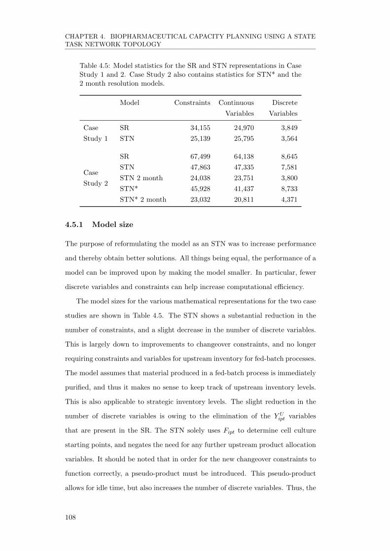
CHAPTER 4. BIOPHARMACEUTICAL CAPACITY PLANNING USING A STATETASK NETWORK TOPOLOGY
Table 4.5: Model statistics for the SR and STN representations in CaseStudy 1 and 2. Case Study 2 also contains statistics for STN* and the2 month resolution models.
Model Constraints Continuous
Variables
Discrete
Variables
Case
Study 1
SR 34,155 24,970 3,849
STN 25,139 25,795 3,564
Case
Study 2
SR 67,499 64,138 8,645
STN 47,863 47,335 7,581
STN 2 month 24,038 23,751 3,800
STN* 45,928 41,437 8,733
STN* 2 month 23,032 20,811 4,371
4.5.1 Model size
The purpose of reformulating the model as an STN was to increase performance
and thereby obtain better solutions. All things being equal, the performance of a
model can be improved upon by making the model smaller. In particular, fewer
discrete variables and constraints can help increase computational efficiency.
The model sizes for the various mathematical representations for the two case
studies are shown in Table 4.5. The STN shows a substantial reduction in the
number of constraints, and a slight decrease in the number of discrete variables.
This is largely down to improvements to changeover constraints, and no longer
requiring constraints and variables for upstream inventory for fed-batch processes.
The model assumes that material produced in a fed-batch process is immediately
purified, and thus it makes no sense to keep track of upstream inventory levels.
This is also applicable to strategic inventory levels. The slight reduction in the
number of discrete variables is owing to the elimination of the Y Uipt variables
that are present in the SR. The STN solely uses Fipt to determine cell culture
starting points, and negates the need for any further upstream product allocation
variables. It should be noted that in order for the new changeover constraints to
function correctly, a pseudo-product must be introduced. This pseudo-product
allows for idle time, but also increases the number of discrete variables. Thus, the
108
CHAPTER 4. BIOPHARMACEUTICAL CAPACITY PLANNING USING A STATETASK NETWORK TOPOLOGY
STN should perform better as the number of products increases, thereby reducing
the impact of the extra pseudo-product. This can be seen in the table, where
the STN in case study 1 shows a 7.4% reduction in discrete variables, whereas
in case study 2 the reduction is 12.3%, reflecting the fact that there are 6 rather
than 4 products.
Owing to the way the STN is formulated, it is possible to change the time
resolution. The resolution was changed to two months to see whether it could
help improve performance. Having a resolution of two months means that each
time period is 60 days rather than 30 days, and thus an 8 year capacity plan
becomes 48 time periods rather than 96. This drastically reduces the size of
the model, as shown in Table 4.5. The performance implications are discussed
later. The STN with extra features (STN*) has a greater number of discrete
variables, since the retrofitting variables LUipt and LD
jpt have been moved from
being continuous to discrete. This is so that the retrofitting constraints work
correctly for the downtime that is now applied when retrofitting takes place.
Although there are now new constraints regarding retrofitting, there are fewer
surrounding the scheduling of production in the CMO, thus the overall number
of constraints is slightly reduced. Again, the two month resolution of STN* also
shows a dramatic reduction in model size.
4.5.2 Performance comparison
The performance of the models are shown in Table 4.6. In addition to the objec-
tive value, the actual cost, and customer service level (CSL) are also shown. The
actual cost excludes penalty costs arising from backlogs and strategic inventory
deficits. It is shown so that it is easier to determine how or why a particular
solution is better than another. For example, in case study 1 the SR and STN
rolling time horizons have very similar objective values, and yet the actual cost
of the STN 4/1 RH is 35 units less. This means that for a similar objective value,
it has found a cheaper solution that can still manufacture enough material to
minimise penalty costs to a similar degree at the SR 4/1 RH. Showing the actual
cost can also help identify when a solution or case study is heavily influenced by
109

CHAPTER 4. BIOPHARMACEUTICAL CAPACITY PLANNING USING A STATETASK NETWORK TOPOLOGY
Table 4.6: Computational results for the SR and STN for the two case studies.Case Study 2 also includes results for the 2 month resolution model, and the STNwith extra features (STN*). Optimality gaps for the rolling time horizons (RH)are for each sub-problem. Actual cost excludes penalty costs. Customer servicelevel (CSL) is also shown.
Model Obj Actual
Cost
CSL (%) Time (s) Optimality
(%)
Case
Study 1
SR 3667 2939 100 10000 12.8
STN 3574 2760 100 10000 8.4
SR 4/1 RH 3528 2631 100 3455 3
STN 4/1 RH 3533 2596 100 1362 3
STN 4/1 RH 3,2 3515 2564 100 1651 3,2a
Case
Study 2
SR 5230 3213 97.4 36000 9.4
STN 5029 2996 97.7 650 5
SR 4/1 RH 5045 3050 97.4 2440 5
STN 2 month 5689 3006 96.9 196 5
STN* 3158 2620 100 36000 13.7
STN* 4/1 RH 3249 3044 100 6611 5b
STN* 2 month 3157 2969 100 32958 5b Last sub-problem was run to 2% optimalityb Last sub-problem timed-out after 3600 seconds at 7.1 % optimality
penalty costs.
Case study 1 proved to be problematic for both the SR and STN, but the
STN has a tighter model and thus reached greater optimality. The STN also
obtained a superior solution, both in terms of the objective value and the actual
cost. A rolling time horizon was used to see whether better solutions could be
achieved by breaking the problem into smaller sub-problems. Each sub-problem
was optimised to 3% optimality, and as explained in the previous chapter, only
optimises 4 years at any given point. The STN 4/1 RH is faster than SR 4/1
RH, but does not provide a better objective value. It was noticed that the
STN was a tighter model, and the lower bound moved rapidly in the last sub-
problem, not allowing enough time for superior solutions to arise. Therefore,
the rolling horizon procedure was modified slightly so that the last sub-problem
was optimised to 2% optimality, and this resulted in a better solution, with only
a slight increase in computational effort. This modification was not applied to
110
CHAPTER 4. BIOPHARMACEUTICAL CAPACITY PLANNING USING A STATETASK NETWORK TOPOLOGY
the SR 4/1 RH because it was already running substantially slower. Figure 4.3a
shows the optimisation profile for the SR and STN, clearly demonstrating that
at any given point in time, the STN provides not only a better solution but also
greater optimality.
Case study 2 has a larger number of products and facilities, and therefore
the models are greater in size (as seen in Table 4.5). It would be expected,
therefore, that the performance of the models for this case study would be worse,
but as seen in Table 4.6 it is actually better in terms of the optimality gap
being achieved. This can be attributed to the fact that there are large penalty
costs being applied to backlogs, as observed by the large discrepancy between
actual costs and objective values. Since the penalty costs overshadow the other
smaller costs, the optimality gap is closed faster. In case study 1, the CSL
was 100%, and thus there were no backlogs. Case study 2 has approximately
97% CSL (excluding STN* which has new features which help alleviate capacity
bottlenecks). Nevertheless, despite obtaining better optimality, the SR was still
intractable, timing out after 10 hours of optimisation. The STN, however, reached
5% optimality in just over 10 minutes, obtaining a much better solution in the
process. To improve upon the SR’s performance, a rolling time horizon was used
once again. Whilst the rolling time horizon did improve upon the SR (both in
terms of objective value and time), it did not outperform the standalone STN.
Figure 4.3b shows the performance profile for the SR and STN in case study
2, and it can be noticed that for a given solution, the STN provided a tighter
lower bound and therefore greater optimality. The SR only slowly improved upon
its solution and lower bound, and from 8000 seconds until 36,000 seconds (only
the first 10,000 seconds are shown in the figure), the model barely improves the
optimality or objective value. It should be noted that the solution from the STN
was subsequently used to fix the optimisation for the SR to ensure that it was
indeed a feasible solution for both models.
To see whether the STN’s performance could be improved further, a two
month resolution version was run. As explained previously, this would mean that
the model would be approximately half the size, and thus would hopefully run
111
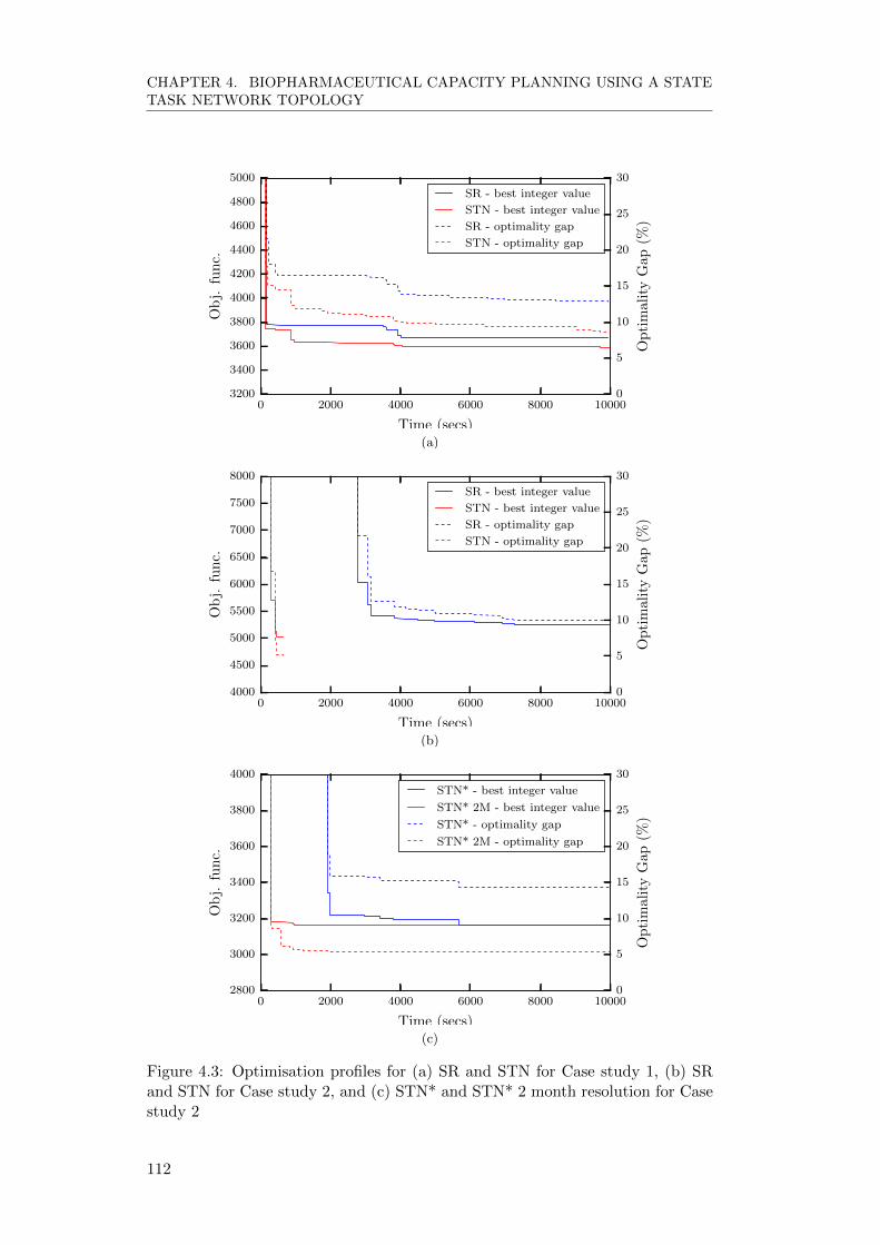
CHAPTER 4. BIOPHARMACEUTICAL CAPACITY PLANNING USING A STATETASK NETWORK TOPOLOGY
0 2000 4000 6000 8000 10000
Time (secs)
3200
3400
3600
3800
4000
4200
4400
4600
4800
5000
Ob
j.fu
nc.
SR - best integer value
STN - best integer value
SR - optimality gap
STN - optimality gap
0
5
10
15
20
25
30
Op
tim
alit
yG
ap(%
)
(a)
0 2000 4000 6000 8000 10000
Time (secs)
4000
4500
5000
5500
6000
6500
7000
7500
8000
Ob
j.fu
nc.
SR - best integer value
STN - best integer value
SR - optimality gap
STN - optimality gap
0
5
10
15
20
25
30
Op
tim
alit
yG
ap(%
)
(b)
0 2000 4000 6000 8000 10000
Time (secs)
2800
3000
3200
3400
3600
3800
4000
Ob
j.fu
nc.
STN* - best integer value
STN* 2M - best integer value
STN* - optimality gap
STN* 2M - optimality gap
0
5
10
15
20
25
30
Op
tim
alit
yG
ap(%
)
(c)
Figure 4.3: Optimisation profiles for (a) SR and STN for Case study 1, (b) SRand STN for Case study 2, and (c) STN* and STN* 2 month resolution for Casestudy 2
112

CHAPTER 4. BIOPHARMACEUTICAL CAPACITY PLANNING USING A STATETASK NETWORK TOPOLOGY
faster. Table 4.6 shows how the STN two month model does indeed run much
faster, but at the expense of a worse solution. The issue with a two month reso-
lution is that when capacity becomes limited, the model is less flexible, and thus
cannot produce enough to meet demand or strategic inventory targets. Originally,
the STN had a CSL of 97.7%, thus it was already clear that there were issues
with backlogs. The two month resolution compounds this problem, resulting in a
greater objective value. When penalty costs are removed, it can be seen that the
actual costs for the STN and STN two month resolution are relatively similar,
but the CSL has dropped for the two month resolution model. Allowing the op-
timisation to continue for longer, and thus achieve greater optimality, would not
help in this situation. When comparing the two month resolution (2M) to the
one month resolution (1M) model, the solution from 2M was converted offline so
that it was compatible with 1M, and then 1M was fixed with that solution (apart
from idle time) and optimised. This second optimisation is incredibly quick, and
reaches 0.1% optimality within seconds, but it is necessary to ensure the solutions
are feasible, and that the costs are calculated correctly.
The second half of the results from case study 2 contain solutions from the
STN with new features (STN*). One of the features which had a great impact on
the objective value is that of initial inventory levels. Having initial inventory levels
meant that the backlogs which occurred near the beginning of the capacity plan
no longer existed, and therefore the penalty costs no longer applied. However,
this did not mean that the optimisation was faster. Indeed, STN* only reached
13.7% optimality after 10 hours. This is consistent with case study 1, where
the 100% CSL meant no backlog penalties, and greater optimality gaps. Whilst
it could be argued that STN* had a greater number of discrete variables than
the STN, this is unlikely to be the main cause of the performance bottleneck.
It may be that without large penalty costs, the optimisation procedure finds it
difficult to quickly differentiate between solutions, making it hard to tighten the
lower bound and obtain better objective values. This is confirmed with the STN*
2 month resolution model (STN* 2M), which has a smaller model size than the
original STN, and yet requires much longer to reach 5% optimality. A comparison
113

CHAPTER 4. BIOPHARMACEUTICAL CAPACITY PLANNING USING A STATETASK NETWORK TOPOLOGY
between the STN* and the STN* 2M can be seen in Figure 4.3c, and an important
point to bear in mind is that although the STN* 2M required a long time to reach
5% optimality, the actual solution never changed from 1500 seconds onwards, and
the optimality gap at that point was already approximately 5.5%. Thus is was a
slow tightening of the lower bound which allowed it to reach termination point.
It is a similar story for the STN*, which reached its best solution after almost
6000 seconds.
Interestingly, although the objective values are almost identical for the STN*
and the STN* 2M, the STN* had a much lower actual cost (that is, the cost
excluding penalty factors). Examining the Gantt charts (Figure 4.4) revealed
that owing to the greater fine-grain control of production that the one month
resolution has, STN* was able to eliminate the use of facility i3, and therefore
the fixed costs for i3 were no longer being applied. The STN* 2M, however, did
require the use of i3. The product which was most problematic from a capacity
perspective was p1, and this product has a 150 day cell culture. With a one
month resolution, this means 5 time periods are used for the cell culture. With
a two month resolution, 3 time periods are required, each 2 months long. This
means that each cell culture for this product requires an allocation of 6 months
rather than the 5 months in the STN*, resulting in problems with backlogs.
The STN* 2M combats this situation by using i3, but this incurs a large fixed
cost. The STN* 2M did however save on cost by using an existing facility i6
for the production of antibodies, rather than build a new facility as per the
STN*. Thus a hybrid between the STN* and the STN* 2M would provide the
best solution. Whilst the actual cost of the STN* is lower, there were greater
penalties attributed to strategic inventory levels, hence why the objective values
between the one month and two month models are similar. A rolling time horizon
was used with the STN*, but it did not achieve a better solution. This could
be down to the fact that when optimising for the first 4 years, it chooses to use
i3 so as to minimise strategic inventory level penalties. The fixed cost is not
as great, since it is only applied for 4 years at this stage. When expanding the
optimisation to 5 years and above, the first years are fixed, thus i3 will continue
114

CHAPTER 4. BIOPHARMACEUTICAL CAPACITY PLANNING USING A STATETASK NETWORK TOPOLOGY
(a) STN
(b) STN*
(c) STN* 2 month resolution
Figure 4.4: Comparison of Gantt charts for Case Study 2. Facilities i6 - i10
and the CMO can only be used by fed-batch processes. Since these do not haveupstream and downstream decoupling, it is not shown in the figures.
115

CHAPTER 4. BIOPHARMACEUTICAL CAPACITY PLANNING USING A STATETASK NETWORK TOPOLOGY
-2000.00 -1500.00 -1000.00 -500.00 0.00 500.00
Backlogs
Transport
Licence
Retrofitting
CMO
Cap. Exp.
Inventory
Variable
Strat. Inv.
Fixed
Cost deviation
Backlogs
Transport
Licence
Retrofitting
CMO
Cap. Exp.
Inventory
Variable
Strat. Inv.
Fixed
(a) STN (b) STN*
(c)
Figure 4.5: Cost breakdown between the STN and the STN with new features(STN*) in Case Study 2. Cost deviations are shown in (c), where positive valuesrepresent places where STN* has a greater cost.
to be used, but now the fixed costs associated with it will be extrapolated for a
greater number of years, thus increasing overall cost.
4.5.3 Effect of new features on production planning
Comparing the Gantt charts of the STN* to the STN shows how the new features
influence the solutions. First of all, initial inventory levels remove the need for
facility i3. Secondly, the retrofitting downtime constraints have meant that it is
no longer optimal to start manufacturing p4 in facility i1. Instead, the demand
for p4 has been met in part by facility i7 and a CMO. This is made possible by the
STN*’s feature of being able to use a CMO for multiple products simultaneously.
116
CHAPTER 4. BIOPHARMACEUTICAL CAPACITY PLANNING USING A STATETASK NETWORK TOPOLOGY
In effect, it would be like having one CMO from years 3-8 (producing p4 in
years 3-4, and p5 in years 5-8), and another CMO used just in year 5 for p6.
A breakdown of the costs between the STN and the STN* is shown in Figure
4.5. It confirms that the majority of the cost difference between the two models
stems from backlog penalties in the STN. It also shows that fixed costs form
the majority of the overall cost in both models, with the STN* having lower
fixed costs in absolute terms for the reasons outlined earlier. The higher capital
expenditure is owing to the construction of facility i7.
Upon examination of the results, it seems that the model size is not a good
indication of computational time required. It would appear that the penalty costs
and overall spare capacity has a large impact on how quickly the optimality gap
can be narrowed. It is not straightforward to determine what the penalty cost
parameters should be, since if they are too small, the model will allow backlogs
unnecessarily. If they are too large, the model solves very quickly, but not neces-
sarily with the best real solution. Spare capacity (especially if there is symmetry
between various manufacturing options) means it is more likely that penalties
will have less impact (since demands can be met on time), and thus causes the
optimisation to slow down as very similar solutions are analysed.
4.5.4 Decentralised manufacturing
The previous sections discussed the use of a state-task network design to improve
performance. Furthermore, new features were included into the model to enhance
the model’s realism and accuracy. The subsequent sections continue to explore
these new features and answer fundamental questions surrounding production
planning.
One of the decisions that must be made when considering how to expand in-
house capacity, is the kind of facility to be built. A company could choose to build
either multiple smaller facilities or one large facility. The case study presented
in this chapter has one large facility which contains 6 x 2000 L bioreactors, and
two smaller facilities each containing 2 x 2000 L bioreactors. The downstream
suites are sized per batch, and are therefore the same size between facilities.
117

CHAPTER 4. BIOPHARMACEUTICAL CAPACITY PLANNING USING A STATETASK NETWORK TOPOLOGY
For mammalian cell cultures, the upstream process is often the bottleneck, with
durations of around 10-14 days. Downstream processes generally take far less
time, and thus having multiple bioreactors function in parallel could greatly help
eliminate the upstream bottleneck. The cost to build the large facility, i7, is 180
RMU, whereas each small facility costs 90 RMU. In this section, the decision was
made to keep production in-house, and hence the use of a CMO was disabled.
(a)
(b)
Figure 4.6: Effect of changeover times for fed-batch cultures on decision to builda centralised or decentralised capacity network. Changeover times are (a) 1 weekand (b) 2 weeks. Facility i7 is large, and i8 − i9 are small.
Figure 4.6 shows how the decision to build one large facility was chosen as
the optimal solution in terms of cost with a standard changeover duration of
118

CHAPTER 4. BIOPHARMACEUTICAL CAPACITY PLANNING USING A STATETASK NETWORK TOPOLOGY
one week. The objective values were {Cost: 3526, CSL: 100%, Inventory: 84%}.
The existing facility i6 was retrofitted to allow for the production of p5, and the
new large facility i7 was used to continue the production of p4 and p6. As soon
as the changeover times for antibody production were increased to two weeks,
the option of building a single large facility was unable to meet market demand
unless facility i1 was also retrofitted. Since retrofitting is expensive, the cheaper
option now was to build two smaller facilities (Figure 4.6b). Utilising two smaller
facilities allows for greater flexibility and fewer changeovers, hence it is able to
cope with the increased changeover duration without any further retrofitting of i1.
In addition, since i6 does not need to be retrofitted for the production of p5, the
other antibody products can continue to use the facility during year three, leading
to higher inventory levels. The objective values for this solution were {Cost: 3576,
CSL: 100%, Inventory: 88%}. The increased cost when compared to the large
facility with one week changeovers is due to the fact that having two smaller
facilities requires more fixed cost than one large facility, which accumulates over
the 5-6 years that they are used.
Importantly, whilst the large facility had greater upstream capacity than the
two smaller facilities combined, it was not able to cope with small changes in oper-
ating procedures in this particular case study. The more robust option was build-
ing two small facilities. The capital expenditure was the same, but in conjunction
with i6, three products could be manufactured simultaneously, rather than two
in the large option. This greater flexibility increased the solution’s robustness to
uncertainty. If there were unplanned downtime due to a contamination or equip-
ment failure, and one of the suites had to be closed down temporarily, having
an extra suite would help satisfy demands. It should be noted that although not
shown here, the scenario with the CMO re-enabled was also run. The findings
were that the model still preferred using two smaller facilities (given two week
changeover durations). The overall cost was slightly greater using a CMO, be-
cause the higher costs of producing in a CMO over 8 years outweighed the capital
expenditure of building smaller facilities.
119

CHAPTER 4. BIOPHARMACEUTICAL CAPACITY PLANNING USING A STATETASK NETWORK TOPOLOGY
4.5.5 Retrofitting a multi-purpose facility
In the previous chapter, constraints were incorporated into the model so that
when the upstream suite of facility i1 was retrofitted for fed-batch production,
the original perfusion-based products could no longer be manufactured. This was
due to the fact that the 2000 L bioreactors used for the antibodies would be too
large to move in and out of a suite. Additionally, if the equipment were moved
from the suite, it would still need to be stored elsewhere. However, the impact
of these operating restrictions can have huge consequences on capacity planning,
as shown in Figure 4.7.
In this figure, it is assumed that the large facility i7 was built, and that owing
to an increase in changeover times, retrofitting i1 was required. The option of
using a CMO was removed, since there was the desire to keep production in-house.
When retrofitting for fed-batch processes blocks any further perfusion cell
cultures, the manufacturing of products p2 − p3 must be conducted in facility i5.
This facility must be built, hence large capital expenditure must be employed.
If, on the other hand, i1 was truly multi-purpose and allowed both fed-batch and
perfusion mode processes to be run, then the capital expense of building a new
facility could be avoided. One may argue that a 30 day changeover time is not
enough to move all the equipment. This is a valid concern, but can be addressed
in two ways.
First, when retrofitting the facility, one could have in mind that the equipment
cannot be moved, and thus enough space must be made available to house both
sets of equipment. In this way, switching between products would not require
extensive moving of large equipment, but extra cleaning and validation may be
required to prove to regulatory bodies that good manufacturing practices are
being maintained.
The second option is to use single-use bioreactors (SUB) for the fed-batch cell
cultures. In this case study, the bioreactors are 2000 L in size, which is within the
size limitations of SUBs. Using disposable equipment will negate the difficulty
of moving large stainless steel bioreactors, and could allow the suite to become
120

CHAPTER 4. BIOPHARMACEUTICAL CAPACITY PLANNING USING A STATETASK NETWORK TOPOLOGY
(a)
(b)
Figure 4.7: Multi-purpose facility options for i1: (a) retrofitting for fed-batch pro-cesses restricts subsequent perfusion production, (b) fully multi-purpose facilitywith 30 day changeovers between different process modes.
multi-purpose.
The implications of restricting a suite to only one process mode can be large
if it then forces the construction of new facilities. Building new facilities increases
the risk a company adopts. Demand is only a forecast, and if the market demand
reduces then the company will be left with an expensive, under-utilised facility.
Retrofitting an existing facility eliminates much of this risk, and can also be
performed quicker. The total costs for 4.7a and 4.7b are 3828 RMU and 3587
RMU respectively, highlighting the fact that in this case study, the better option
121
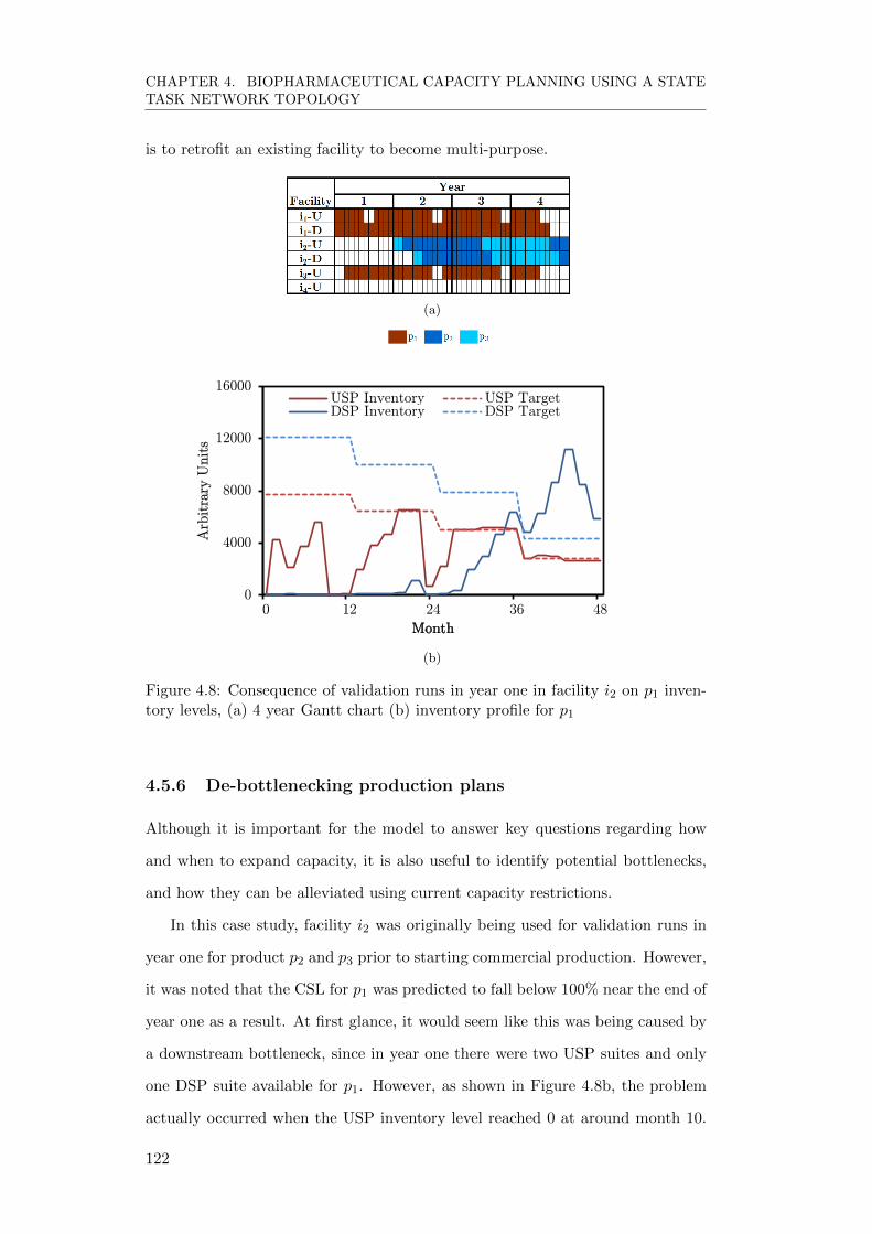
CHAPTER 4. BIOPHARMACEUTICAL CAPACITY PLANNING USING A STATETASK NETWORK TOPOLOGY
is to retrofit an existing facility to become multi-purpose.
(a)
0
4000
8000
12000
16000
0 12 24 36 48
Arb
itra
ry U
nit
s
Month
USP Inventory USP TargetDSP Inventory DSP Target
0
4000
8000
12000
16000
0 12 24 36 48
Arb
itra
ry U
nit
s
Month
USP Inventory USP TargetDSP Inventory DSP Target
(b)
Figure 4.8: Consequence of validation runs in year one in facility i2 on p1 inven-tory levels, (a) 4 year Gantt chart (b) inventory profile for p1
4.5.6 De-bottlenecking production plans
Although it is important for the model to answer key questions regarding how
and when to expand capacity, it is also useful to identify potential bottlenecks,
and how they can be alleviated using current capacity restrictions.
In this case study, facility i2 was originally being used for validation runs in
year one for product p2 and p3 prior to starting commercial production. However,
it was noted that the CSL for p1 was predicted to fall below 100% near the end of
year one as a result. At first glance, it would seem like this was being caused by
a downstream bottleneck, since in year one there were two USP suites and only
one DSP suite available for p1. However, as shown in Figure 4.8b, the problem
actually occurred when the USP inventory level reached 0 at around month 10.
122
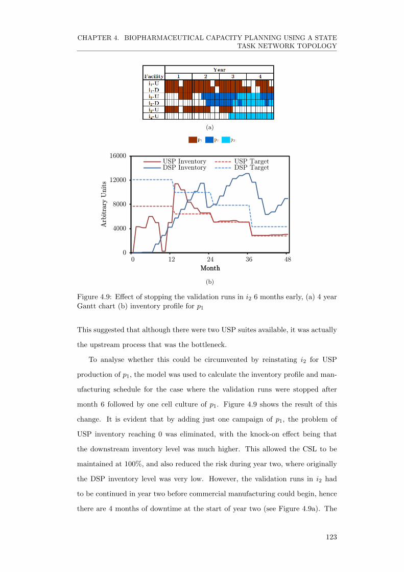
CHAPTER 4. BIOPHARMACEUTICAL CAPACITY PLANNING USING A STATETASK NETWORK TOPOLOGY
(a)
0
4000
8000
12000
16000
0 12 24 36 48
Arb
itra
ry U
nit
s
Month
USP Inventory USP TargetDSP Inventory DSP Target
(b)
Figure 4.9: Effect of stopping the validation runs in i2 6 months early, (a) 4 yearGantt chart (b) inventory profile for p1
This suggested that although there were two USP suites available, it was actually
the upstream process that was the bottleneck.
To analyse whether this could be circumvented by reinstating i2 for USP
production of p1, the model was used to calculate the inventory profile and man-
ufacturing schedule for the case where the validation runs were stopped after
month 6 followed by one cell culture of p1. Figure 4.9 shows the result of this
change. It is evident that by adding just one campaign of p1, the problem of
USP inventory reaching 0 was eliminated, with the knock-on effect being that
the downstream inventory level was much higher. This allowed the CSL to be
maintained at 100%, and also reduced the risk during year two, where originally
the DSP inventory level was very low. However, the validation runs in i2 had
to be continued in year two before commercial manufacturing could begin, hence
there are 4 months of downtime at the start of year two (see Figure 4.9a). The
123

CHAPTER 4. BIOPHARMACEUTICAL CAPACITY PLANNING USING A STATETASK NETWORK TOPOLOGY
effect of this is that i4 is required for the production of p3, the demand for which
could previously be met solely in i2. Facility i4 needs to be built, hence this
change increases the capital expenditure of the company, albeit keeping the CSL
at 100%. In reality, a company could choose to delay the launch of a product
or reduce the amount it will supply to the market in the first few years, thereby
removing the need to build a new facility, or at least delaying the construction.
Here, it was assumed that the demands and launch date remained unchanged.
Nevertheless, the model allowed the user to quickly determine whether a slight
change to the production plan could help eliminate a bottleneck, and calculate the
repercussions this would have on the production of other products in subsequent
years.
4.6 Summary
This chapter has demonstrated the performance benefits of reformulating the
mathematical model as a state-task network. The STN was able to outperform
the SR in all cases, and in one of the case studies the standalone full-scale STN
proved superior to the SR using a rolling time horizon. Issues still remain when
the customer service level is close to 100%, and penalty costs have less impact on
the objective value. A method which could eliminate the use of penalty costs may
help with these issues, and could provide a more realistic production schedule.
The model presented here also demonstrated the use of extra features which
make the scheduling more realistic from a production perspective. Retrofitting
downtime has a large effect on determining optimal solutions. Allowing a CMO to
be modelled as multiple third-parties rather than one facility, with minimum an-
nual production limits, also adds more functionality and flexibility to the model.
In addition to the monthly resolution model, a two month time resolution
was also used with the STN. Although faster, the solutions obtained from the
two month model were not as good when capacity was nearing its limit. When
capacity is not a large bottleneck, the two month model provides equally good
solutions in much less time, reaching optimality targets in the process.
124

CHAPTER 4. BIOPHARMACEUTICAL CAPACITY PLANNING USING A STATETASK NETWORK TOPOLOGY
The advantages of using a decentralised production plan were discussed in
the context of an industrial case study. The increased manufacturing flexibility
of having multiple smaller facilities improved the robustness of the production
plans should any unforeseen downtime occur.
The impact that different retrofitting options had on capacity planning was
considered for multi-purpose facilities. The implications of preventing a facility
from being truly multi-purpose, were an increase in capital expenditure, and
greater risk associated with unused capacity in new builds.
Finally, the model was used to identify bottlenecks in production, and allowed
the user to quickly determine how these bottlenecks could be removed. The
impact this would have on the manufacturing of other products could then be
analysed rapidly.
The next chapter discusses the use of a multi-objective model, which can help
a production team determine which solution is best for them given their own
strategic criteria.
125

CHAPTER 4. BIOPHARMACEUTICAL CAPACITY PLANNING USING A STATETASK NETWORK TOPOLOGY
4.7 Nomenclature
Indices
i, j suite (alias)p, p′ product (alias)t, θ time period (alias))y year
Sets
I, J suitesIp, Jp suites which produce product pIt, Jt suites available in time period tIowned, Jowned suites which are ownedIretrofit, J retrofit suites which have retrofitting capabilitiesP productsP p products which are produced by perfusionP r products which are real (not pseudo-product)Pi, Pj products which are produced by suite i or jT time periodsTy time periods which are part of year yTi, Tj time periods which suite i or j are available inYt year which contains time period t
Scalars
H time horizon (days)Havailabley maximum utilisation time in a year (days)
wcost cost to discard a unit of any product
126

CHAPTER 4. BIOPHARMACEUTICAL CAPACITY PLANNING USING A STATETASK NETWORK TOPOLOGY
Parameters
δp backlog penalty costεt discount factorζUp upstream product shelf-life (time periods)
ζDp downstream product shelf-life (time periods)
ηUip upstream product batch cost
ηDjp downstream product batch cost
κi facility investment costλip licence feesλUip retrofitting cost for upstream product
λDjp retrofitting cost for downstream product
ρip storage costρcarryip carry of inventory cost
τp perfusion cell culture duration (time periods)τ retrofiti , τ retrofit
j retrofitting duration (time periods)
τbuildi suite construction duration (time periods)τqcp time required for QCQA (time periods)τ starti starting time period for facility iDpt demand of product p at time period t (units vary)Dlastp the time period containing the last demand of product p
Ipenaltyp penalty applied when strategic inventory is not met
IU,specialipt USP additional inventory (e.g., initial levels)
ID,specialjpt DSP additional inventory (e.g., initial levels)
Imin,Upt USP strategic inventory level
Imin,Dpt DSP strategic inventory level
nρipθ number of USP batches that are produced in period θ of cell culture
nUip′p number of USP batches subtracted due to changeover time
nDjp′p number of DSP batches subtracted due to changeover time
nD,maxjpt maximum number of DSP batches that can be produced in a time period
nD,minjpt minimum number of DSP batches that should be produced in a time period
qcostij cost to transport intermediate material from facility i to j
rUip USP batch rate (batches/day)
rDjp DSP batch rate (batches/day)
ucost,Ui USP fixed cost
ucost,Dj DSP fixed cost
xloadp downstream lot sizes (units vary)
xmin,CMOpy minimum amount of p that should be produced in a CMO in a yearxUip USP batch output (units vary)
xDjp DSP batch output (units vary)
Binary Variables
Fipt 1 if a new cell culture of product p is started in facility i over period tY Djpt 1 if product p is produced in suite j over period t
LUipt 1 if retrofitting for product p in suite i starts at t
LDjpt 1 if retrofitting for product p in suite j starts at t
127

CHAPTER 4. BIOPHARMACEUTICAL CAPACITY PLANNING USING A STATETASK NETWORK TOPOLOGY
Integer Variables
BUipt number of USP batches produced in suite i over time t of product p
BDjpt number of DSP batches produced in suite j over time t of product p
Positive Variables
AUipt, ADjpt 1 if USP or DSP suite is available
Aretrofit,Uipt 1 if USP suite has been retrofitted
Aretrofit,Djpt 1 if DSP suite has been retrofitted
Ait 1 if suite has been builtCjpy amount of product p produced in outsourced suites in year yIUipt, I
Djpt USP/DSP inventory level
Idev,Uipt USP inventory amount deviating from strategic level
Idev,Djpt DSP inventory amount deviating from strategic level
Kit 1 if investment to construct suite i took place in period tLipt, Ljpt 1 if licence payment for product p starts at t in suite i or jQijpt flow of material from USP to DSP suiteSjpt sales amount of product p (units vary)Wjpt amount of product p which is wasted (units vary)UUi , U
Dj 1 if suite i or j have been used
Xjpy 1 if product p is produced in suite j in year yZUip′pt, Z
Djp′pt 1 if there is a changeover from p′ → p in USP or DSP suites
∆pt demand not met
Free Variables
Cost manufacturing cost (to be minimised)
128

Chapter 5
Multi-Criteria Strategic
Planning for
Biopharmaceutical Production
5.1 Introduction
Biopharmaceutical companies face increasing pressure to meet market demands
for multiple commercial therapeutics whilst minimising costs and capital expendi-
ture. Different stakeholders will place emphasis on separate and often conflicting
objectives, such as maximising customer service levels, posing various capacity
planning challenges.
A tool that can incorporate various strategic criteria into the optimisation
process is advantageous not only in terms of operational cost savings that result
from optimal manufacturing schedules, but also in that it provides a clearer
understanding of how uncertainty within the manufacturing environment can
affect the robustness of a solution.
Hence this chapter builds upon the long-term production planning model de-
scribed in the previous chapter by incorporating multiple objectives, including
minimising the manufacturing cost whilst maintaining high customer service lev-
els and strategic inventory targets. Two multi-objective methods are compared to
129

CHAPTER 5. MULTI-CRITERIA STRATEGIC PLANNING FORBIOPHARMACEUTICAL PRODUCTION
one another: goal programming and the ε-constraint method, and the advantages
of using the ε-constraint method are discussed.
An industrial case study is presented with results showing how these factors,
including varying the changeover times, can impact the different objectives and
manufacturing schedules, highlighting some of the key challenges within strategic
decision-making in the biopharmaceutical industry.
5.2 Problem Definition
The problem being discussed here is that of minimising the total cost of biophar-
maceutical production over a finite time horizon. A diverse portfolio of different
product types must be optimally allocated across a network of different facilities,
each with their own manufacturing capabilities. The robustness of a solution is
an important aspect to production planning, and thus methods are required to
identify those solutions which would provide a more consistent schedule given
various strategic criteria.
5.2.1 Multi-objective criteria
Often there are multiple conflicting objectives that must be met in biopharma-
ceutical production planning. For example, a company may wish to minimise
the total cost and capital expenditure, while simultaneously satisfying market
demands and maintaining strategic inventory levels. Whilst these concerns can
be included in a single-objective model by applying penalty costs to any unmet
criteria (for example, penalising backlogs), this method does not allow a user to
easily determine how the different objectives interact with one another.
A multi-objective model can help a decision maker analyse the effects various
objectives have on manufacturing decisions. In addition, by generating a set of
optimal solutions one can determine which production plan is best suited to the
company’s attitude to risk.
130

CHAPTER 5. MULTI-CRITERIA STRATEGIC PLANNING FORBIOPHARMACEUTICAL PRODUCTION
5.3 Mathematical Formulation
This chapter adds a multi-objective component to the STN mathematical for-
mulation outlined in the previous chapter. Three objectives were investigated:
cost, customer service level, and strategic inventory levels. Two techniques were
used to obtain multi-objective solutions, goal programming and the ε-constraint
method.
5.3.1 Goal programming
The weighted goal programming method used here has been described in relation
to biopharmaceutical capacity planning elsewhere (Lakhdar et al., 2007). One
of the main reasons for using goal programming is that it is easy and intuitive
to use for a decision maker, since placing targets on objectives and assigning
weights is an understandable process. However, although easy to understand,
sometimes it is not straightforward to determine which targets and weights to
use, and this can have a large effect on the solutions found. There is also the issue
of Pareto optimality, whereby one of the objectives in a solution provided by goal
programming could be improved further without degrading any other objective.
Although there are methods for fixing solutions so that they are Pareto optimal
(Tamiz et al., 1999), there is still the problem of determining the full Pareto set
of solutions.
Three key variables are introduced into the model. The goal target for
each goal g, GTg, the goal level, GLg, and the deviations from the goal tar-
gets, GDg,dev. There are two deviations that are possible, positive and negative,
whereby both GDg,pos and GDg,neg are positive variables.
Cost
The total cost is equal to all operating costs and capital expenditure. More
precisely, it includes inventory costs, variable costs, fixed costs, transport costs,
waste costs, facility investment, retrofitting costs, and licence costs. The following
equation sums these costs to form the goal level GLcost. Individual components
131

CHAPTER 5. MULTI-CRITERIA STRATEGIC PLANNING FORBIOPHARMACEUTICAL PRODUCTION
of the equation are listed in the previous chapter.
GLcost = IC + V C + FC + TC +WC + FI +RC + LC (5.1)
Customer service level
The customer service level (CSL) is calculated as a percentage of demand that is
met on time. The parameter P dt represents the number of products that have a
demand in time period t, and is used to divide the summation of demand met, so
that the CSL never exceeds 100%. GLTcsl,t represents the goal level for customer
service level achieved for all products that have a demand in time period t. This
variable is then summed over all time periods which have demands present, T d,
and divided by the cardinality of T d (that is, the total number of time periods
which have a demand present). This then forms the goal level for CSL, GLcsl.
GLTcsl,t = 100×∑
p|Dpt>0
( ∑j∈Jp∩Jt
Sjpt
)−∆p,t−1
Dpt/P dt ∀ t (5.2)
GLcsl =
∑t∈T d
GLTcsl,t
card(T d)(5.3)
Strategic inventory level
The inventory level for downstream production is often desired to be at a certain
target level so that any problems with production have less of an impact on
meeting demand. Here, the amount of inventory that is within the target level
for a given time period is represented by GLTinv,t. The actual goal level, GLinv,
is then calculated by summing GLTinv,t over all time periods which have an
inventory target, T inv. A value of 100% means that inventory targets have been
132

CHAPTER 5. MULTI-CRITERIA STRATEGIC PLANNING FORBIOPHARMACEUTICAL PRODUCTION
met for all products over all time periods.
GLTinv,t = 100×( ∑p|Imin,D
pt >0
(1−
Idev,Dpt
Imin,Dpt
))/P inv
t ∀ t (5.4)
GLinv =
∑t∈T inv
GLTinv,t
card(T inv)(5.5)
Normalisation constraints
The difference between the goal targets, GTg, and goal levels, GLg, is used to
calculate the deviation variables GDg,pos and GDg,neg.
GLg −GTg = GDg,pos −GDg,neg ∀g (5.6)
In order to create an objective function which considers all goal deviations,
they must first be normalised. The normalised deviations, GDnormg,dev are calculated
as follows:
GDnormg,dev = 100×
GDg,dev
GTg∀g,dev (5.7)
Finally, the weighted sum of these goal deviations is used in the objective
function, where wg,dev represents the weight assigned to a particular goal devia-
tion.
minimise∑g,dev
wg,devGDnormg,dev (5.8)
The full goal programming model consists of Equations 4.1-4.58, and 5.1 - 5.8.
5.3.2 ε-constraint method
One of the drawbacks of weighted goal programming is that of determining the
weights and targets. Even once established, it is difficult to obtain a set of Pareto
solutions using goal programming. Here, we describe the ε-constraint method,
133

CHAPTER 5. MULTI-CRITERIA STRATEGIC PLANNING FORBIOPHARMACEUTICAL PRODUCTION
and how it is applied to our model. The method used here is called AUGMECON2
and has been described in other work (Mavrotas and Florios, 2013).
The ε-constraint method works by converting all but one of the objectives into
constraints, and then using an iterative process (see Figure 5.1) to find optimal
values for all objectives. In general terms, to find the optimal solution x over p
objective functions, f1(x) to fp(x), we use the following:
Problem P:
max(f1(x) + eps× (s2/r2 + 10−1s3/r3 + . . .+ 10−(p−2)sp/rp)
)st
fk(x)− sk = ek k = 2 . . . p
x ∈ S (5.9)
where:
S is the feasible region of the original problem
sk are non-negative slack variables
ek = lbk + ik × stepk
lbk is the lower bound for objective k
stepk = rk/gk: the step for objective k
rk is the range for objective k
gk is the number of intervals for objective k
ik is the counter for objective k for parametric variation of the constraint’s RHS
eps is a very small number (10−3)
For this piece of work, the three objectives considered are cost, CSL and
strategic inventory targets, represented by f1(x), f2(x) and f3(x) respectively.
Since Equation 5.9 is formulated as a maximisation problem, the sign of the
objective value for cost is inversed.
The method first creates a payoff table from which it determines a range of
values for CSL and inventory targets. It splits these ranges into equally spaced
134

CHAPTER 5. MULTI-CRITERIA STRATEGIC PLANNING FORBIOPHARMACEUTICAL PRODUCTION
START
Create payoff table (lexmaxfk(x), k = 1 . . . p)
Set lower bounds lbk for k = 2 . . . p
Calculate ranges rk for k = 2 . . . p
Divide rk into gk intervals (set number ofgridpoints = gk + 1)
Initialise counters: ik = 0 fork = 2 . . . p, np = 0
ip = ip + 1
ip−1 = ip−1 + 1
i2 = i2 + 1
Solve problem P
Feasible?
np = np + 1Calculate b =int(s2/step2)
i2 = i2 + b
i2 = g2 i2 < g2?
i2 = 0
ip−1 < gp−1?
ip−1 = 0
ip < gp?
END
yes
no no
yes
yes
no
no
yes
Figure 5.1: Flowchart of the ε-constraint method used in this work. Adaptedfrom Mavrotas and Florios (2013)
135
CHAPTER 5. MULTI-CRITERIA STRATEGIC PLANNING FORBIOPHARMACEUTICAL PRODUCTION
points. It then picks the first point for inventory targets, and the first point
for CSL. These points become the respective ek values in Equation 5.9. The
optimisation as per Equation 5.9 is run, whereby the lowest cost is found given
that the two other objectives are at least as big as their ek values. It then changes
the ek for CSL to the next point in its range, and repeats the optimisation. This
is repeated until the CSL range is exhausted, at which point its ek is reset to the
first point, and the inventory target ek is incremented to the next point in its
range. The CSL ek is again varied through its range. This process is repeated
until ek has been varied for all values in both ranges. This method, therefore,
provides solutions for all combinations of CSL and inventory targets within a
range and predefined number of grid points.
The individual objectives are calculated as per Equations 5.1-5.5. Equations
4.1-4.58 from the previous chapter form the remaining constraints. These equa-
tions, together with Equation 5.9, form the ε-constraint model.
5.4 Illustrative Example
The case study presented here consists of 6 products and 10 facilities. Prod-
uct information regarding process data and costs are shown in Table 5.1. The
costs for antibody products p4−p6 were assimilated using discussions with indus-
try and the commercial software BioSolve (Biopharm Services, Chesham, UK).
Three types of antibodies were included: monoclonal antibodies (mAbs), frag-
ment antigen binding (Fab) fragments, and antibody drug conjugates (ADCs).
For in-house production, capital costs were removed from the calculations, since
capital expenditure associated with equipment purchases and retrofitting were in-
cluded separately in our model. Fixed costs in our model include labour, utilities,
cleaning, insurance and taxes. The costs derived from consumables and materials
constitute the variable costs. In order to calculate the costs for CMOs, capital
charges were added to the previous costs, and the resulting cost was increased
by 50% to reflect the additional expense of using a CMO. Costs for p1 − p3 were
obtained from industrial discussion and used a variable:fixed cost ratio which
136

CHAPTER 5. MULTI-CRITERIA STRATEGIC PLANNING FORBIOPHARMACEUTICAL PRODUCTION
Table 5.1: Process data for products in Case Study 3
Product
p1 p2 p3 p4 p5 p6
Product typeBlood-
factor
Blood-
factor
Blood-
factormAb Fab ADC
Process data
USP
Fermentation mode Perfa Perfa Perfa FBb FBb FBb
Cell culture duration (days) 180 120 60 10 3 10
Harvest (AUc/day) 120 130 490 - - -
QC/QA time (days) 60 30 30 - - -
DSP
Lot size (AUc) 320 450 1000 6 2 6
Duration (days) 1.5 1.5 1.5 1.5 3.5 3.5
Cost data
USP
Variable (RMUd/AUc) 0.019 0.019 0.019 0.004 0.002 0.004
Fixed (RMUd/year) 14.4 14.4 14.4 3.5 3.9 3.5
DSP
Variable (RMUd/AUc) 0.018 0.018 0.018 0.02 0.026 0.156
Fixed (RMUd/year) 9 9 9 4.7 7.1 5.6
CMO (RMUd/AUc) - - - 0.42 0.54 0.64a Perfusion b Fed-batch c Arbitrary units d Relative monetary units
reflected the expected annual output.
The manufacturing capability matrix and upstream bioreactor scale are shown
in Table 5.2. It should be noted that p5 uses E. coli as its expression system,
and thus it would be unlikely that it would be able to be produced in the same
suite as a product using mammalian cells. Great effort would be required to
show that there is a clear segregation between the processes, and that there is
no sharing of equipment. The cost and risk involved in convincing regulatory
bodies are likely to outweigh any benefit from having dual production, especially
since the incentive of sharing equipment would be non-existent. With careful
consideration, it may be possible to convince regulatory authorities by using
disposable equipment, but this would probably be limited to toxicology or phase I
137
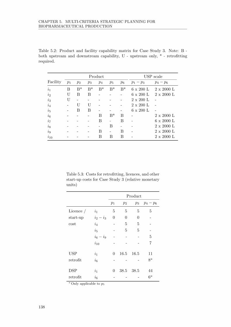
CHAPTER 5. MULTI-CRITERIA STRATEGIC PLANNING FORBIOPHARMACEUTICAL PRODUCTION
Table 5.2: Product and facility capability matrix for Case Study 3. Note: B -both upstream and downstream capability, U - upstream only, * - retrofittingrequired.
Product USP scaleFacility p1 p2 p3 p4 p5 p6 p1 − p3 p4 − p6
i1 B B* B* B* B* B* 6 x 200 L 2 x 2000 Li2 U B B - - - 6 x 200 L 2 x 2000 Li3 U - - - - - 2 x 200 L -i4 - U U - - - 2 x 200 L -i5 - B B - - - 6 x 200 L -i6 - - - B B* B - 2 x 2000 Li7 - - - B - B - 6 x 2000 Li8 - - - - B - - 2 x 2000 Li9 - - - B - B - 2 x 2000 Li10 - - - B B B - 2 x 2000 L
Table 5.3: Costs for retrofitting, licences, and otherstart-up costs for Case Study 3 (relative monetaryunits)
Product
p1 p2 p3 p4 − p6
Licence /
start-up
cost
i1 5 5 5 5
i2 − i3 0 0 0 -
i4 - 5 5 -
i5 - 5 5 -
i6 − i9 - - - 5
i10 - - - 7
USP
retrofit
i1 0 16.5 16.5 11
i6 - - - 8a
DSP
retrofit
i1 0 38.5 38.5 44
i6 - - - 6a
a Only applicable to p5
138
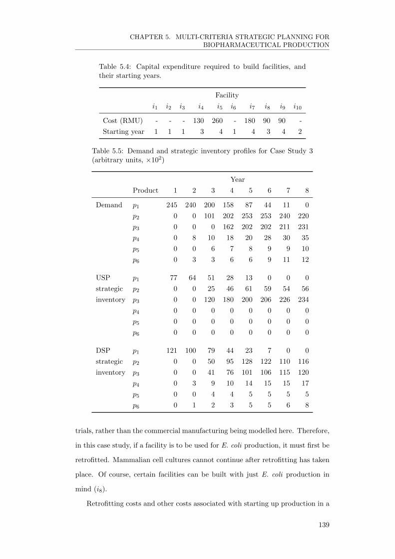
CHAPTER 5. MULTI-CRITERIA STRATEGIC PLANNING FORBIOPHARMACEUTICAL PRODUCTION
Table 5.4: Capital expenditure required to build facilities, andtheir starting years.
Facility
i1 i2 i3 i4 i5 i6 i7 i8 i9 i10
Cost (RMU) - - - 130 260 - 180 90 90 -
Starting year 1 1 1 3 4 1 4 3 4 2
Table 5.5: Demand and strategic inventory profiles for Case Study 3(arbitrary units, ×102)
Year
Product 1 2 3 4 5 6 7 8
Demand p1 245 240 200 158 87 44 11 0
p2 0 0 101 202 253 253 240 220
p3 0 0 0 162 202 202 211 231
p4 0 8 10 18 20 28 30 35
p5 0 0 6 7 8 9 9 10
p6 0 3 3 6 6 9 11 12
USP
strategic
inventory
p1 77 64 51 28 13 0 0 0
p2 0 0 25 46 61 59 54 56
p3 0 0 120 180 200 206 226 234
p4 0 0 0 0 0 0 0 0
p5 0 0 0 0 0 0 0 0
p6 0 0 0 0 0 0 0 0
DSP
strategic
inventory
p1 121 100 79 44 23 7 0 0
p2 0 0 50 95 128 122 110 116
p3 0 0 41 76 101 106 115 120
p4 0 3 9 10 14 15 15 17
p5 0 0 4 4 5 5 5 5
p6 0 1 2 3 5 5 6 8
trials, rather than the commercial manufacturing being modelled here. Therefore,
in this case study, if a facility is to be used for E. coli production, it must first be
retrofitted. Mammalian cell cultures cannot continue after retrofitting has taken
place. Of course, certain facilities can be built with just E. coli production in
mind (i8).
Retrofitting costs and other costs associated with starting up production in a
139

CHAPTER 5. MULTI-CRITERIA STRATEGIC PLANNING FORBIOPHARMACEUTICAL PRODUCTION
facility are shown in Table 5.3. The cost to build a facility, and the year that it
can begin being used, is shown in Table 5.4. Demand and strategic inventory lev-
els are shown for all products in Table 5.5. In this model, material from upstream
production of antibody-based products is not stored, but instead processed im-
mediately in a purification suite. Therefore, there are no USP strategic inventory
levels for p4 − p6. Generally, the strategic levels are a function of demand in
subsequent years, and are seen as a safety margin should unforeseen events, such
as earthquakes, occur.
5.5 Results
5.5.1 Comparing multi-objective methods
The first section of the results will discuss the merits of using the ε-constraint
method over weighted goal programming for multi-objective problems. As men-
tioned earlier, one of the problems with using weighted goal programming is that
it is difficult to obtain a complete set of Pareto solutions. Two ways in which a
user could attempt to generate a set of solutions are (a) varying the weights, and
(b) varying the targets. In contrast, the ε-constraint method eliminates the need
of assigning weights or targets, and instead uses an iterative process to obtain a
set of Pareto optimal solutions.
Figure 5.2 shows the different set of solutions generated for two objectives by
goal programming methods and the ε-constraint method. The two objectives are
total cost and customer service level (CSL). In Figure 5.2a, the cost and CSL
target were kept constant (750 RMU and 100% respectively) and the weights
were varied as follows. The weight for cost was kept at 1, and CSL was varied
as 1.2, 1.4, 1.6, 1.8, 2, 3, ... , 8, 9. This was then repeated the other way round.
Hence, in total 25 optimisations were conducted (24 from varying the weights,
and one base case with the weights set at 1:1). Despite the fact that a wide range
of weights were explored, the set of solutions obtained was not evenly dispersed.
Instead, there are clusters of solutions around five distinct points. This shows
two things: (a) the value of the weights chosen by the decision maker has a
140
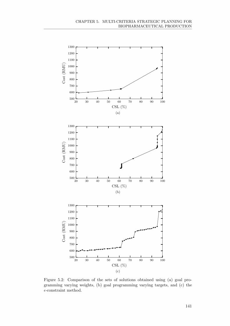
CHAPTER 5. MULTI-CRITERIA STRATEGIC PLANNING FORBIOPHARMACEUTICAL PRODUCTION
20 30 40 50 60 70 80 90 100
CSL (%)
500
600
700
800
900
1000
1100
1200
1300
Cos
t(R
MU
)
(a)
20 30 40 50 60 70 80 90 100
CSL (%)
500
600
700
800
900
1000
1100
1200
1300
Cos
t(R
MU
)
(b)
20 30 40 50 60 70 80 90 100
CSL (%)
500
600
700
800
900
1000
1100
1200
1300
Cos
t(R
MU
)
(c)
Figure 5.2: Comparison of the sets of solutions obtained using (a) goal pro-gramming varying weights, (b) goal programming varying targets, and (c) theε-constraint method.
141

CHAPTER 5. MULTI-CRITERIA STRATEGIC PLANNING FORBIOPHARMACEUTICAL PRODUCTION
real impact on the solutions obtained, and (b) varying the weights is not a good
method of generating a Pareto set.
The effect of varying the targets on the set of solutions obtained was inves-
tigated next. Here, the weights were kept constant at 1:1. The CSL target was
also kept constant, at 100%. The cost target was varied from 500 RMU to 1250
RMU, with steps of 10 RMU. Hence, 76 optimisations were conducted. As Fig-
ure 5.2b shows, whilst there is a slight improvement in the number of different
solutions obtained, most are not useful since they are just dominated solutions.
For example, at 95% CSL there is a set of solutions ranging from approximately
1000-1150 RMU. Obviously, for the same CSL, the solution with the lowest cost is
preferable. This clearly illustrates the problem of Pareto inefficiencies generated
using weighted sum goal programming. It should be noted that no attempt was
made to repair the solutions to ensure Pareto optimality, since the added com-
putational time required to accomplish this was deemed unnecessary given that
other multi-objective techniques were available. In addition, even if solutions
were repaired, it would be difficult to obtain an even distribution of solutions
along the curve. The other issue visible in the figure is that no solutions with a
CSL lower than approximately 60% were attained. This is due to the fact that
the CSL target was kept constant at 100%, and highlights the problem of varying
weights and targets to obtain a complete Pareto set.
The ε-constraint method used in this work should in theory be able to generate
an evenly distributed set of Pareto optimal solutions. The CSL range used was 20-
100%, with 48 evenly distributed optimisations. Figure 5.2c shows the resulting
curve, and it is clear to see that the solutions obtained are superior to those from
the goal programming method, since for any given CSL, the same or a lower
cost is achieved. Owing to the nature of the method, the solutions are evenly
distributed along the curve. However, Pareto optimality is only guaranteed if the
individual optimisations are run to 100% optimality. Owing to computational
reasons, this could not be achieved here. However, since the optimality gap used
here was just 1%, the majority of the solutions generated were very close to being
Pareto efficient, with only a couple of noticeable outliers (namely, around 25%
142

CHAPTER 5. MULTI-CRITERIA STRATEGIC PLANNING FORBIOPHARMACEUTICAL PRODUCTION
CSL).
The computational effort of obtaining the set of solutions presented in Figure
5.2 varies between methods. All three methods were executed for a three year
capacity plan, with goal programming methods run to 3% optimality and the ε-
constraint method to 1%. Changing the weights in goal programming resulted in a
total time of 5310 seconds, changing the targets resulted in 3150 seconds, and the
ε-constraint method required 2280 seconds. Given the fact that the ε-constraint
method was not only quicker, but also provided a more evenly distributed set
of solutions with greater Pareto efficiency, it seems to be a better choice when
facing multi-objective problems like the one presented here.
5.5.2 Effect of variability on multi-objective criteria
The use of a multi-objective model is demonstrated through the heat maps pre-
sented in this section. Three objectives are considered: cost, customer service
level, and strategic inventory levels. Using the ε-constraint method, the CSL
and inventory level objectives are split into 8 points each, ranging from 70-100%.
Thus, up to 64 optimisations are used to generate each heat map. Sometimes
fewer than 64 optimisations are run, because the particular ε-constraint method
used here can skip optimisations which provide no additional information. Here,
the capacity plan is for three years and considered antibody production only.
The colours on the heat maps represent total cost, which includes manufacturing
costs and capital expenditure, amongst other costs (see Equation 5.1).
The changeover times between products are sometimes not known precisely
until personnel have had the experience of manufacturing the products for them-
selves. Different operating practices and personnel experience levels can have an
effect on the changeover times. Equipment sizes can vary widely between prod-
ucts and will also have an impact on the time, to the point where it may even
be deemed infeasible to switch between certain products. In addition, if the seed
train is to be produced in the same suite as the production-scale bioreactor, then
the changeover times could easily be extended to 3-4 weeks for a mammalian cell
culture at a 2000 L commercial scale.
143
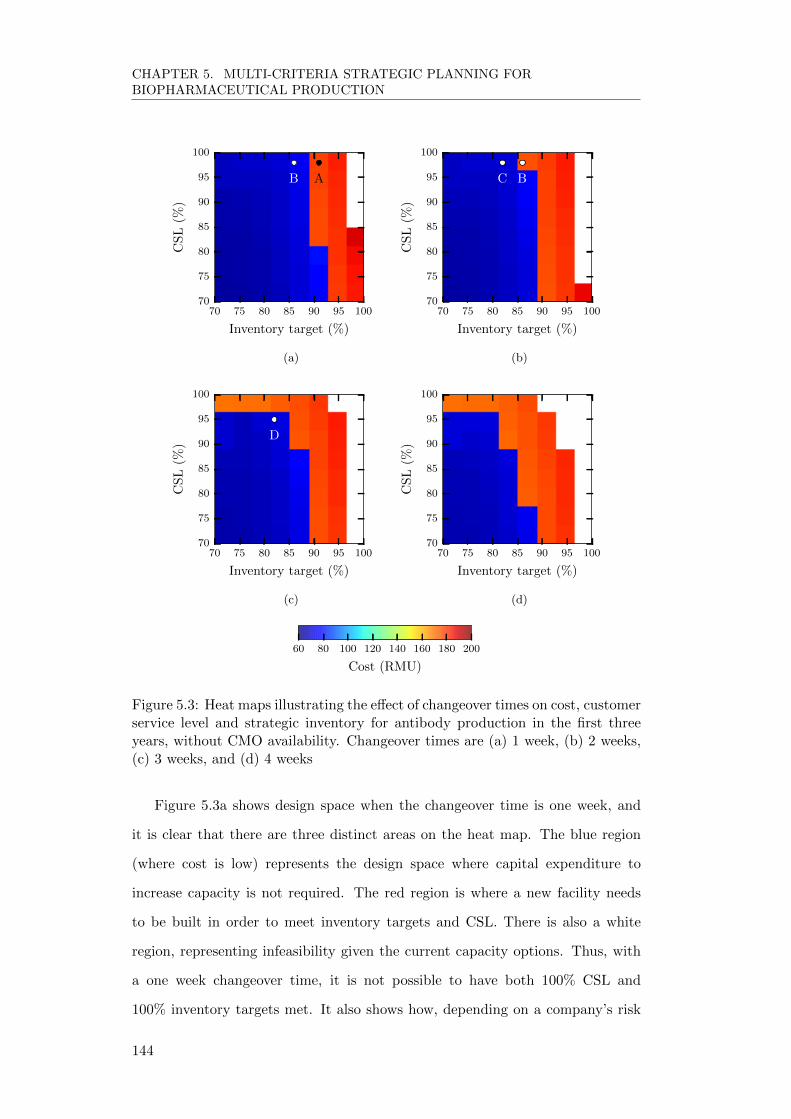
CHAPTER 5. MULTI-CRITERIA STRATEGIC PLANNING FORBIOPHARMACEUTICAL PRODUCTION
70 75 80 85 90 95 100
Inventory target (%)
70
75
80
85
90
95
100
CS
L(%
)AB
(a)
70 75 80 85 90 95 100
Inventory target (%)
70
75
80
85
90
95
100
CS
L(%
)
BC
(b)
70 75 80 85 90 95 100
Inventory target (%)
70
75
80
85
90
95
100
CS
L(%
)
D
(c)
70 75 80 85 90 95 100
Inventory target (%)
70
75
80
85
90
95
100C
SL
(%)
(d)
60 80 100 120 140 160 180 200
Cost (RMU)
Figure 5.3: Heat maps illustrating the effect of changeover times on cost, customerservice level and strategic inventory for antibody production in the first threeyears, without CMO availability. Changeover times are (a) 1 week, (b) 2 weeks,(c) 3 weeks, and (d) 4 weeks
Figure 5.3a shows design space when the changeover time is one week, and
it is clear that there are three distinct areas on the heat map. The blue region
(where cost is low) represents the design space where capital expenditure to
increase capacity is not required. The red region is where a new facility needs
to be built in order to meet inventory targets and CSL. There is also a white
region, representing infeasibility given the current capacity options. Thus, with
a one week changeover time, it is not possible to have both 100% CSL and
100% inventory targets met. It also shows how, depending on a company’s risk
144

CHAPTER 5. MULTI-CRITERIA STRATEGIC PLANNING FORBIOPHARMACEUTICAL PRODUCTION
tolerance, one could drastically reduce cost by moving from point A to point B.
The customer service level remains constant between the points, but the inventory
target is reduced by 5%. This will negate the need to build a new facility and
hence reduce capital expenditure by 90 RMU.
At first glance this seems to be a good trade-off, and worth the risk. However,
if changeover times were to be extended to two weeks (Figure 5.3b), point B can
no longer be maintained without a new facility. If the decision had already been
made to forgo the new build and begin manufacturing at operating point B (with
one week changeovers in mind), then it may be impossible to continue operating
at point B altogether if changeovers became two weeks. This is because there
is a construction time associated with building a facility. Thus a delay in the
construction starting time would alter the design space. However, CSL can still
be kept at 100% by moving to point C, at the expense of reducing inventory levels
even further.
Matters are compounded when the changeover duration is extended to three
weeks (Figure 5.3c). In this case, 100% CSL is not possible unless a new facility
is built, thus if the original strategy was to operate at point B (which is no longer
possible), then the CSL would have to drop to 95%, seen at point D. Of course,
it may also be possible to reduce inventory targets to below 70% and achieve
100% CSL, but here we are assuming that management want to operate within
the design space shown. Finally, four week changeovers are shown in Figure
5.3d. As can be seen from the heat maps, there is a gradual increase in the
infeasible space as changeover times increase. However, so long as a new facility
is built, there will always be the possibility to maintain 100% CSL. Thus, the
less risky option, and potentially better option overall, would be to build a new
facility, and thereby have a more robust manufacturing schedule that can cope
with unexpected downtime or operating changes. It should be noted that these
results disable the use of a CMO. The effect of using a CMO is discussed next,
in the context of titre variation.
Titres often fluctuate throughout the course of commercial manufacturing,
owing to the inherent uncertainty present in biological systems (Stonier et al.,
145
CHAPTER 5. MULTI-CRITERIA STRATEGIC PLANNING FORBIOPHARMACEUTICAL PRODUCTION
2013). There is also the possibility that titres for new products do not meet
expectations as the process is scaled up to commercial manufacturing. As men-
tioned in Chapter 3, there is also the chance that a lower titre cell line is chosen
if it generates fewer host cell impurities and thus allows for easier purification.
Therefore, an analysis on the effect of a ±20% variation in titre for antibody
products is examined in Figure 5.4. The antibody products were chosen because
the case study used generic platform processes for their production, and thus key
variables such as titre may change. The changeover time was kept constant at
one week.
When the titre was reduced by 20%, it became impossible to satisfy demand
and maintain 70% inventory targets using existing facilities (Figure 5.4a). A new
facility had to be built (represented by the red region), but even then it may
be risky should changeover times increase or other factors occur which further
reduce capacity. The base case shown in Figure 5.4b is the same as that shown in
Figure 5.3a. When titres increased by 20% in Figure 5.4c, the infeasible demands
in the base case can now be met with the use of the new facility. The stark
difference between the three figures show the large impact titres have on capacity
requirements and the decisions that must be made accordingly. In Figure 5.3, it
seemed like building a new facility would be sufficient in terms of meeting demand
given uncertain changeover times. When variable titres are considered however,
it may be that it is deemed too risky.
To reduce some of the inherent risk associated with the uncertainty surround-
ing titres and changeover times, one may wish to outsource capacity to a CMO.
Figures 5.4d-5.4f demonstrate how by using a CMO one can satisfy demands and
strategic inventory levels at all times. Notice that the dark blue regions cover the
same areas as those covered in the respective ‘non-CMO’ heat maps, highlight-
ing the fact that the model will use in-house facilities where possible, and only
outsource when using a CMO is cheaper than any other alternative (for example,
building a facility). For this particular case study, it would seem that a CMO
is the least risky option, and also offers a reasonable cost trade-off. It should be
noted that in order to use a CMO, time would be required for technology transfer
146

CHAPTER 5. MULTI-CRITERIA STRATEGIC PLANNING FORBIOPHARMACEUTICAL PRODUCTION
70 75 80 85 90 95 100
Inventory target (%)
70
75
80
85
90
95
100
CS
L(%
)
(a)
70 75 80 85 90 95 100
Inventory target (%)
70
75
80
85
90
95
100
CS
L(%
)
(b)
70 75 80 85 90 95 100
Inventory target (%)
70
75
80
85
90
95
100
CS
L(%
)
(c)
70 75 80 85 90 95 100
Inventory target (%)
70
75
80
85
90
95
100
CS
L(%
)
(d)
70 75 80 85 90 95 100
Inventory target (%)
70
75
80
85
90
95
100
CS
L(%
)
(e)
70 75 80 85 90 95 100
Inventory target (%)
70
75
80
85
90
95
100
CS
L(%
)
(f)
60 80 100 120 140 160 180 200
Cost (RMU)
Figure 5.4: Heat maps illustrating the effect of titre fluctuations on antibodyproduction in the first three years. Titres are (a) -20%, (b) base case, (c) +20%.This is repeated with CMO availability in (d)-(f).
147

CHAPTER 5. MULTI-CRITERIA STRATEGIC PLANNING FORBIOPHARMACEUTICAL PRODUCTION
and negotiating contracts. Hence, if a CMO is to be used, the decision needs to be
made early on. A point to bear in mind is that these figures are showing the best
options available over a three year capacity plan. If the planning horizon were to
be extended to eight years, it may be that building new facilities is actually the
best long-term option.
The multi-objective model can help decision makers determine the best op-
erating points given their risk tolerance and long-term strategy. Variations in
processes or operating procedures can influence the choices made. The results
from this case study suggest that using a CMO is potentially the safest option
for the first few years. There are reasons why a company may not want to use
a CMO however, and thus the figures allow a decision maker to identify points
where capacity bottlenecks could occur.
5.6 Summary
This chapter has explored the use of a multi-objective model in aiding a deci-
sion maker in choosing desired operating points for production planning. Both
goal programming and the ε-constraint method were investigated as ways in
which different solutions could be obtained. The ε-constraint method provided a
more evenly distributed set of solutions, and allowed a user to more easily deter-
mine inflection points where capacity could be affected. Uncertainty surrounding
biopharmaceutical production planning was explored using the multi-objective
model to examine the robustness of solutions, allowing decision makers to iden-
tify the best schedules based on their risk tolerances.
This chapter has shown the merits of developing a tool which can quickly cal-
culate optimal manufacturing schedules based on strategic criteria that a decision
maker may enforce. It can also be easily adapted should one wish to consider
other objectives or scenarios.
148

CHAPTER 5. MULTI-CRITERIA STRATEGIC PLANNING FORBIOPHARMACEUTICAL PRODUCTION
5.7 Nomenclature
Indicesg goal (objective)dev goal deviation
SetsT d time periods which have a demandT inv time periods which have a stategic inventory level
ParametersP invt number of products which have a strategic inventory level at time period tP dt number of products which have a demand at time period tGTg goal targetwg,dev weight assigned to goal deviation
Positive VariablesGLTgt goal level at time period tGDg,dev goal deviation
Free VariablesGLg goal levelGDnorm
g,dev normalised goal deviation
149

CHAPTER 5. MULTI-CRITERIA STRATEGIC PLANNING FORBIOPHARMACEUTICAL PRODUCTION
150
Chapter 6
Conclusions and Future Work
6.1 Introduction
The purpose of this thesis was to develop a framework which can be used to
determine optimal capacity plans for biopharmaceutical production, and allow
an end-user to investigate how uncertain input parameters can affect the result.
In order to accurately model a capacity plan, a biopharmaceutical strategist must
consider the following:
• The process details including yield and duration for upstream and down-
stream production of each product.
• Manufacturing capabilities in each suite, and the network structure regard-
ing transferral of intermediate product.
• Strategic options available to the company regarding capacity expansion,
for example, outsourcing to a CMO or building new facilities.
• The multiple strategic criteria by which a capacity plan is optimised for.
• Financial requirements of manufacturing the therapeutics being modelled.
• Capital expenditure requirements for retrofitting or building facilities.
• Operational constraints between different products.
151

CHAPTER 6. CONCLUSIONS AND FUTURE WORK
• The parameters which demonstrate uncertainty in the manufacturing and
capacity planning stages.
This thesis has addressed all of these features of biopharmaceutical capacity
planning in detail. Results are shown on how uncertainty surrounding CMO cost
and product titres affect the capacity plans in question, and the overall costs over
a finite period of time. The complexity of the model resulted in computational in-
efficiencies which were addressed by reformulating the model. Although the new
formulation was a large improvement over the original model, there were still
computational issues surrounding certain case studies. An extension to this work
would investigate alternative formulations which would improve performance even
further. The multi-criteria nature of biopharmaceutical manufacturing was ad-
dressed via the use of multi-objective optimisation. Three objectives were con-
sidered, with results showing the trade-offs surrounding the costs and risks asso-
ciated with operating at various design points. The number of objectives could
be increased further, but would compound the computational effort required to
obtain sets of optimal solutions. The graphical representation of higher dimen-
sional data would also be more difficult to understand. Lastly, the optimisation
of biopharmaceutical capacity plans is an important aspect to biomanufactur-
ing. As portfolios of products and the number of available manufacturing suites
increase in size, the problem becomes non-trivial to solve. Therefore, computa-
tional tools which intelligently obtain optimal manufacturing schedules, as shown
in this work, is of great relevance to industry.
6.2 Contributions of this thesis
The primary aim of this work is the creation of a mathematical model which
obtains the optimal manufacturing schedules and capacity plans for a portfo-
lio of products displaying different modes of cell-culture, amongst a network of
multi-purpose facilities. Various constraints inherent in biopharmaceutical man-
ufacturing make this computationally difficult. The work conducted to solve this
problem and the contributions of this thesis are outlined below.
152

CHAPTER 6. CONCLUSIONS AND FUTURE WORK
6.2.1 Capacity planning for batch and perfusion bioprocesses
across multiple biopharmaceutical facilities
Chapter 3 describes the development of a novel model which includes both per-
fusion and fed-batch processes in its capacity planning capabilities. In order to
correctly accommodate the differences between different process modes, sequence-
dependent changeovers were introduced, adding further complexity to the model.
The introduction of decoupled upstream and downstream production added fur-
ther flexibility to the model, and more realistically represented biomanufacturing
of perfusion based products.
A rolling time horizon procedure was used to obtain solutions using fewer
computational resources, and was shown to provide capacity plans with lower
overall costs. An industrial case study was analysed using the model to demon-
strate the usefulness of a computational framework that optimises manufacturing
schedules in a holistic manner that considers capital investment.
6.2.2 Biopharmaceutical Capacity Planning using a State Task
Network Topology
Chapter 4 demonstrates the performance improvement obtained by reformulating
the mathematical model into a state task network. Two case studies were used
to show the merits of the reformulation in terms of model size and performance.
In all cases, the state task network (STN) formulation was faster and provided
better solutions.
The STN also added extra features to the model that increased the realism
of the manufacturing schedules. Retrofitting downtime was included, and was
shown to have a large impact on the solutions that were obtained. Increased
flexibility in the way in which CMOs were modelled also changed the optimal
solutions, resulting in cases where multiple CMOs were utilised during periods of
high demand and restricted in-house capacity.
An investigation into the effect of changing the time resolution of the STN to
two months was carried out, and was shown to drastically reduce the computa-
153
CHAPTER 6. CONCLUSIONS AND FUTURE WORK
tional effort required. However, depending on the case study, it did not always
provide better solutions overall.
Various strategic options surrounding how best to expand capacity were in-
vestigated. A decentralised expansion programme was compared to a centralised
programme, and shown to be more robust when increased changeover durations
were introduced. The issue of vastly different equipment in perfusion and fed-
batch processes was examined in terms of retrofitting options. Executive decisions
which prevent a suite from being multi-purpose were shown to be sub-optimal
both in terms of the extra capital expenditure that would be required otherwise,
and the increased risk involved in building new facilities to satisfy demands. Fi-
nally, the model was used to demonstrate its de-bottlenecking capabilities, and
its usefulness in aiding a strategic planner in predicting how small changes in the
manufacturing schedule affect long-term planning.
6.2.3 Multi-Criteria Strategic Planning for Biopharmaceutical
Production
Chapter 5 continued with the development of the STN in Chapter 4 by adding a
multi-objective component that could take into account the multi-criteria aspect
of biomanufacturing. The ε-constraint method was compared to weighted-sum
goal programming, and was shown to be the superior multi-objective method for
generating complete sets of optimal solutions. It was then used to show how
variations in certain input parameters could affect the design space and points at
which capacity expansion was required.
6.3 Recommendations for Future Work
Creating a framework which closely represents the intricate details of biomanu-
facturing is a difficult task. Ways in which the framework developed here could
be extended include:
• Problem features
154

CHAPTER 6. CONCLUSIONS AND FUTURE WORK
• Uncertainty
• Alternative search heuristics
This section discusses how the framework could be extended to consider each
of the above points.
6.3.1 Problem features
The mathematical model presented in this thesis is a close representation of real
biomanufacturing for both perfusion and fed-batch processes. However, there are
areas which could be extended in order to add further realism to the model. One
of the issues with adding more functionality is that the computational effort will
also be increased. Computational complexity is often a limiting factor in deciding
which features to include, and thus new methods of improving the performance
of the model should also be investigated. Some features which would enhance
the model are discussed below.
Timing considerations
This model has used sequence-dependent changeover times to take into account
the additional complexity of switching between fed-batch and perfusion processes.
However, these times cannot exceed one time period, and thus if one wished to
include extra setup times into the model (for example, extended seed train times),
this would not be possible with the current formulation. Changeover times could
be measured in terms of time periods instead of days, but that would not be
a feasible strategy for long-term capacity planning where time periods are one
month or greater. Alternatively, since idle time is considered a pseudo-product
in the STN model, one could enforce downtime associated with changeovers by
starting a campaign of the pseudo-product. This would also require changing
the formulation of the model such that it allows a maximum of two products to
be produced in a time period. A potential reformulation could be taken from
examples of the proportional lot size and scheduling problem, where any unused
time within a time period can be used for scheduling a second product. This
155

CHAPTER 6. CONCLUSIONS AND FUTURE WORK
type of reformulation may also aid with increasing the flexibility of scheduling,
especially when capacity is limited and multiple short campaigns of different
products is required.
The number of time periods in the model has a large effect on computational
efficiency. Efforts were made to reduce the number of time periods by making the
time horizon two months rather than one. Whilst this did help obtain solutions
faster, it led to inferior solutions when capacity was limited. A hybrid model could
be useful in these situations. One model could use monthly time horizons, and
another could use 2 month or quarterly horizons. Then the user can pick which
model should be used in various parts of the 10 year capacity plan. A simple case
would be to say that the finer model should be used at the beginning (perhaps
the first year) when demands are more certain, and then use the less fine model
in subsequent years. A hybrid model could also be used in a more systematic
way. For example, use the fine model for the first year, and for the last 9 years
use the coarse model. If there are any capacity bottlenecks in the subsequent 9
years, rerun the optimisation, but this time using the fine model in the year that
had the bottleneck. This can be repeated until there are no bottlenecks, or until
the entire 10 years is using the fine model. Given the performance improvement
of using a coarser model, this method will not be as computationally expensive
as it may first seem, and could provide better solutions faster in most cases.
Transportation duration was not included in the mathematical model, but
would be an important factor when capacity is tight and intermediate inventory
levels are low. Moving material between countries which are far apart would ob-
viously require time and careful logistic planning. The model could be adapted to
include transportation times by changing Equation 4.45 such that Qijpt becomes
Qijp,t+τ transportij
, where τ transportij is the transportation duration between suites i
and j.
Fixed costs
Currently, fixed costs are assigned to a particular suite a priori, and if that suite
is used, the cost is applied in the objective function. This assumption is valid
156

CHAPTER 6. CONCLUSIONS AND FUTURE WORK
if the fixed costs do not vary much between different products, but otherwise a
different approach may be more suitable. Siganporia et al. (2012) use a model
which calculates the fixed costs dynamically based on which products have been
manufactured in a given suite. However, the performance hit from having extra
constraints was deemed to outweigh the benefit of having this type of fixed cost
model.
Objectives
This work introduced equations which considered objectives including total man-
ufacturing cost, maintaining strategic inventory levels, and maximising customer
service levels. The model could be extended by considering alternative criteria
of interest to a strategic planner. Often, manufacturers prefer to have cam-
paigns of longer duration rather than switching many times between products.
Longer campaigns are easier to manage logistically and can minimise the risk
of cross-contamination. Therefore, an objective which minimises the number of
changeovers could be of interest. Alternatively, one could minimise the amount
of downtime in a year attributed to changeovers, which is perhaps a more intu-
itive way of thinking about the same problem. Companies often have utilisation
targets for their facilities, thus an objective could be introduced which minimises
the distance between the targets and current utilisation levels. Capital expendi-
ture is also high on the agenda for many biopharmaceutical companies, thus an
objective which could minimise investment may also be of interest. In this work,
capital investment is included in the total costs objective, thus moving this to a
separate objective may be a more useful measure of performance, depending on
a company’s priorities.
6.3.2 Uncertainty
Uncertainty has been introduced into this work via the use of scenario based
analysis, whereby input parameters are varied and the model is re-optimised.
Whilst this is a useful technique, one may wish to obtain results which also
have probabilities assigned to them. That is, given a probability distribution
157

CHAPTER 6. CONCLUSIONS AND FUTURE WORK
of demands, one may want to know what the likelihood is of building a new
facility. This is only possible if the input parameters are assigned probabilities.
There are different ways in which uncertainty could be introduced. One method
would be to randomly choose an input parameter’s value based on a probability
distribution, and then run the optimisation. This process is then repeated many
times, such that a set of solutions is obtained, each with probability assigned to
them. Another method would be to obtain a base case solution, and then measure
its robustness by fixing the solution and varying the input parameters. The model
would then be able to determine things such as how likely the customer service
level is to be 100% given uncertain titres.
Another area where the model could be expanded is in considering attrition
rates in clinical trials. The current model assumes that all products in its portfolio
have or will have successfully passed their clinical trials. The development of
biopharmaceutical drugs is inherently risky, with just 10-20% of drug candidates
successfully reaching FDA approved status (Nie, 2015). Therefore, one could
leverage this information to provide capacity plans where the probability of drugs
reaching the market is also considered. In this way, the expected net present value
could be obtained for optimal production plans. However, one of the reasons this
idea was not built upon in this work is because of the added computational
complexity required. The model was already hitting performance bottlenecks, so
adding an extra layer would only deteriorate the situation. If further performance
improvements are found, then including clinical trial attrition rates could be of
interest to biopharmaceutical manufacturers.
6.3.3 Alternative search heuristics
Whilst mathematical programming provides a precise way of defining and solving
complex problems, it can quickly become computationally intractable for larger
problem sizes. Therefore, it may be useful to investigate other intelligent search
techniques for determining optimal manufacturing schedules. Genetic algorithms
are commonly used heuristics, but up till now have not been applied to bio-
pharmaceutical capacity planning. An overview of a genetic algorithm that was
158

CHAPTER 6. CONCLUSIONS AND FUTURE WORK
developed and used in this work is presented in Appendix A. Unfortunately, it
did not provide better or faster solutions that the MILP model. Changing the
chromosome structure or reformulating the way in which a genetic algorithm is
used for capacity planning are two possible ways of improving the algorithm, and
could be the basis of future work.
In summary, the work in this thesis provides a strong base for future work in
the area of developing advanced capacity planning models for the sector.
159

CHAPTER 6. CONCLUSIONS AND FUTURE WORK
160

References
Abara, J. (1989). Applying integer linear programming to the fleet assignment
problem. INTERFACES, 19(4):20–28.
Acuna, J., Hewitt, M., Johnston, R., Kirkland, D., Shikibu, T., and Zhang,
D. (2011). Modelling perfusion processes in biopharmaceutical production.
BioProcess International, 9:52–59.
Adams, C. P. and Brantner, V. V. (2010). Spending on new drug development.
Health Economics, 19(2):130–141.
Amanullah, A., Otero, J. M., Mikola, M., Hsu, A., Zhang, J., Aunins, J., Schreyer,
H. B., Hope, J. A., and Russo, A. P. (2010). Novel micro-bioreactor high
throughput technology for cell culture process development: Reproducibility
and scalability assessment of fed-batch cho cultures. Biotechnology and Bio-
engineering, 106(1):57–67.
Amaro, A. and Barbosa-Povoa, A. (2008). Planning and scheduling of industrial
supply chains with reverse flows: A real pharmaceutical case study. Computers
& Chemical Engineering, 32(11):2606 – 2625.
Amodeo, L., Chen, H., and El Hadji, A. (2007). Multi-objective supply chain
optimization: An industrial case study. In Giacobini, M., editor, Applications
of Evolutionary Computing, volume 4448 of Lecture Notes in Computer Science,
pages 732–741. Springer Berlin Heidelberg.
Ashouri, P. (2011). A Dynamic Simulation Framework for Biopharmaceutical
Capacity Management. PhD thesis, University College London.
161

REFERENCES
Barry, F. (2015). Pfizer considers splitting company or going after M&A.
Bashiri, M., Khorasani, H., and Shiri, M. (2014). Multi objective supply chain
network design considering customer satisfaction. In Industrial Engineering
and Engineering Management (IEEM), 2014 IEEE International Conference
on, pages 923–927.
Benzi, G. and Ceci, A. (1998). The ‘drug value’ in the european pharmaceutical
system. Pharmacological Research, 37(5):333 – 337.
Berning, G., Brandenburg, M., Grsoy, K., Kussi, J. S., Mehta, V., and Tolle,
F.-J. (2004). Integrating collaborative planning and supply chain optimization
for the chemical process industry (i) - methodology. Computers & Chemical
Engineering, pages 913–927.
Blackwell, J., Ransohoff, T. C., and Levine, H. L. (2010). Monoclonal antibody
manufacturing strategies for the 21st century. Pharmaceutical Outsourcing,
11:28–35.
Blum, C. and Li, X. (2008). Swarm Intelligence: Introduction and Application,
volume Swarm Intelligence in Optimization. Springer.
Cacciuttolo, M. (2007). Perfusion or fed-batch? A matter of perspective. Cell
culture and upstream processing, page 173184.
Castro, P. M., Grossmann, I. E., and Novais, A. Q. (2006). Two new continuous-
time models for the scheduling of multistage batch plants with sequence depen-
dent changeovers. Industrial & Engineering Chemistry Research, 45(18):6210–
6226.
Chinneck, J. W. (2000). Practical optimization: A gentle introduction.
Clincke, M.-F., Molleryd, C., Zhang, Y., Lindskog, E., Walsh, K., and Chotteau,
V. (2013). Very high density of cho cells in perfusion by ATF or TFF in WAVE
bioreactor. Part I. Effect of the cell density on the process. Biotechnology
Progress, 29:754767.
162
REFERENCES
Colvin, M. and Maravelias, C. T. (2010). Modeling methods and a branch and
cut algorithm for pharmaceutical clinical trial planning using stochastic pro-
gramming. European Journal of Operational Research, 203(1):205 – 215.
Corporation, G. D. (2012). CPLEX 12 Solver Manual.
Dantzig, G. B. (1951). Maximization of a linear function of variables subject to
linear inequalities. In Koopmans, T., editor, Activity Analysis of Production
and Allocation. Wiley, New York.
Darby-Dowman, K. and Wilson, J. M. (2002). Developments in linear and integer
programming. The Journal of the Operational Research Society, 53(10):pp.
1065–1071.
DiMasi, J. A. and Grabowski, H. G. (2007). The cost of biopharmaceutical R&D:
is biotech different? Managerial and Decision Economics, 28(4-5):469–479.
Dorigo, M. (1992). Optimization, Learning and Natural Algorithms. PhD thesis,
Dipartimento di Elettronica, Politecnico di Milano, Italy.
Dorigo, M. and Gambardella, L. M. (1997). Ant colony system: A cooperative
learning approach to the traveling salesman problem. IEEE Transactions on
Evolutionary Computation, 1:53–66.
Dorigo, M., Maniezzo, V., Colorni, A., Dorigo, M., Dorigo, M., Maniezzo, V.,
Maniezzo, V., Colorni, A., and Colorni, A. (1991). Positive feedback as a
search strategy. Technical report.
Dreo, J. (2006). http://en.wikipedia.org/wiki/File:Aco_branches.svg.
Edwards, J. (2011). Patent cliff losses mean eli lilly must acquire or be acquired.
Eraslan, E. and Derya, T. (2010). Daily newspaper distribution planning with
integer programming: an application in turkey. Transportation Planning and
Technology, 33(5):423–433.
Ernst & Young (2015). Beyond borders - Biotechnology Industry Report 2015.
163
REFERENCES
Farid, S. S. (2007). Process economics of industrial monoclonal antibody manu-
facture. Journal of Chromatography B, 848(1):8 – 18.
Foo, F., Karri, S., Davies, E., Titchener-Hooker, N., and Dunnill, P. (2001).
Biopharmaceutical process development: Part i, information from the first
product generation. Pharmaceutical Technology Europe, 13(6):58+60+62–64.
cited By (since 1996) 8.
Gatica, G., Papageorgiou, L., and Shah, N. (2003a). Capacity planning under
uncertainty for the pharmaceutical industry. Chemical Engineering Research
and Design, 81(6):665 – 678.
Gatica, G., Shah, N., and Papageorgiou, L. G. (2003b). An aggregation approach
for capacity planning under uncertainty for the pharmaceutical industry. Foun-
dations of Computer-Aided Process Operations, 4:245–248.
George, E., Titchener-Hooker, N. J., and Farid, S. S. (2007). A multi-criteria
decision-making framework for the selection of strategies for acquiring bio-
pharmaceutical manufacturing capacity. Computers & Chemical Engineering,
31(8):889 – 901. 7th World Congress of Chemical Engineering.
George, E. D. and Farid, S. S. (2008a). Stochastic combinatorial optimization ap-
proach to biopharmaceutical portfolio management. Industrial & Engineering
Chemistry Research, 47(22):8762–8774.
George, E. D. and Farid, S. S. (2008b). Strategic biopharmaceutical portfolio
development: An analysis of constraint-induced implications. Biotechnology
Progress, 24(3):698–713.
Goldberg, D. (1989). Genetic Algorithms in Search, Optimization, and Machine
Learning. Addison-Wesley Professional.
Guillen, G. and Grossmann, I. (2010). A global optimization strategy for the
environmentally conscious design of chemical supply chains under uncertainty
in the damage assessment model. Computers & Chemical Engineering, 34(1):42
– 58.
164
REFERENCES
Guillen, G., Mele, F., Bagajewicz, M., Espuna, A., and Puigjaner, L. (2005).
Multiobjective supply chain design under uncertainty. Chemical Engineering
Science, 60(6):1535 – 1553.
Guntsch, M. and Middendorf, M. (2001). Pheromone modification strategies for
ant algorithms applied to dynamic TSP. In Proceedings of the EvoWorkshops
on Applications of Evolutionary Computing, pages 213–222, London, UK, UK.
Springer-Verlag.
Guntsch, M. and Middendorf, M. (2003). Solving multi-criteria optimization
problems with population-based ACO. In Proceedings of the 2nd international
conference on Evolutionary multi-criterion optimization, EMO’03, pages 464–
478, Berlin, Heidelberg. Springer-Verlag.
Habib, S. J. and Marimuthu, P. N. (2010). Optimized capacity planning and per-
formance measurement through OPNET modeler. In International Conference
on Computer Applications and Industrial Electronics.
Hwang, C. and Masud, A. (1979). Multiple Objective Decision Making - Methods
and Applications: A State of the Art Survey, volume 164 of Lecture Notes in
Economics and Mathematical Systems. Springer-Verlag.
Inman, P. and Hawkes, A. (2011). Pfizer to close factory with loss of 2,400 jobs
as manufacturing soars.
Kantorovich, L. V. (1960). Mathematical methods of organizing and planning
production. Management Science, 6(4):pp. 366–422.
Karmarkar, N. (1984). A new polynomial-time algorithm for linear programming.
Combinatorica, 4:373–395. 10.1007/BF02579150.
Kelley, B. (2009). Industrialization of mab production technology: the biopro-
cessing industry at a crossroads. mAbs, 1(5):443–452.
Klee, V. and Minty, G. J. (1972). How good is the simplex algorithm? In Third
Sympos. (Univ. California, CA, ., editor, Inequalities, III, pages 159–175, New
York. Academic Press.
165
REFERENCES
Kondili, E., Pantelides, C., and Sargent, R. (1993). A general algorithm for short-
term scheduling of batch operations - I. MILP formulation. Computers &
Chemical Engineering, 17(2):211 – 227. An International Journal of Computer
Applications in Chemical Enginnering.
Ku, H. M. and Karimi, I. A. (1991). Scheduling algorithms for serial multiproduct
batch processes with tardiness penalties. Computers & Chemical Engineering,
15(5):283 – 286.
Kux, L. (2012). Prescription drug user fee rates for fiscal year 2013. Federal
Register, 77:45639–45643.
Lakhdar, K. and Papageorgiou, L. G. (2008). An iterative mixed integer optimi-
sation approach for medium term planning of biopharmaceutical manufacture
under uncertainty. Chemical Engineering Research and Design, 86(3):259 –
267.
Lakhdar, K., Savery, J., Papageorgiou, L., and Farid, S. S. (2007). Multiobjective
long-term planning of biopharmaceutical manufacturing facilities. Biotechnol-
ogy Progress, 23(6):1383–93.
Lakhdar, K., Zhou, Y., Savery, J., Titchener-Hooker, N. J., and Papageorgiou,
L. G. (2005). Medium term planning of biopharmaceutical manufacture using
mathematical programming. Biotechnology Progress, 21(5):1478–1489.
Lakshmikanthan, J. (2007). Outsourcing: Biologics manufacturing: The CMO
advantage. BioPharm International, 20.
Langer, E. S. (2011). Survey examines trends in the outsourcing relationship.
BioPharm International, 24:26–33.
Lazaro, M., na, A. E., and Puigjaner, L. (1989). A comprehensive approach
to production planning in multipurpose batch plants. Computers & Chemical
Engineering, 13(9):1031 – 1047.
Lipsky, M. S. and Sharp, L. K. (2001). From idea to market: the drug approval
process. American Board of Family Practice, 14:362–367.
166

REFERENCES
Lorigeon, T., Billaut, J.-C., and Bouquard, J.-L. (2002). A dynamic programming
algorithm for scheduling jobs in a two-machine open shop with an availability
constraint. The Journal of the Operational Research Society, 53(11):pp. 1239–
1246.
Lundy, M. and Mees, A. (1986). Convergence of an annealing algorithm. Math-
ematical Programming, 34:111–124. 10.1007/BF01582166.
Maravelias, C. T. and Grossmann, I. E. (2001). Simultaneous planning for new
product development and batch manufacturing facilities. Industrial & Engi-
neering Chemistry Research, 40(26):6147–6164.
Marichal-Gallardo, P. A. and Alvarez, M. M. (2012). State-of-the-art in down-
stream processing of monoclonal antibodies: Process trends in design and val-
idation. Biotechnology Progress, 28(4):899–916.
Mavrotas, G. (2009). Effective implementation of the epsilon-constraint method
in multi-objective mathematical programming problems. Applied Mathematics
and Computation, 213(2):455–465.
Mavrotas, G. and Florios, K. (2013). An improved version of the augmented
ε-constraint method (augmecon2) for finding the exact pareto set in multi-
objective integer programming problems. Applied Mathematics and Computa-
tion, 219(18):9652 – 9669.
Merkle, D., Middendorf, M., and Schmeck, H. (2000). Ant colony optimization for
resource-constrained project scheduling. In IEEE Transactions on Evolutionary
Computation, pages 893–900. Morgan Kaufmann.
Metropolis, N., Rosenbluth, A. W., Rosenbluth, M. N., Teller, A. H., and Teller,
E. (1953). Equation of State Calculations by Fast Computing Machines. J.
Chem. Phys., 21:1087–1092.
Meuwly, F., Weber, U., Ziegler, T., Gervais, A., Mastrangeli, R., Crisci, C.,
Rossi, M., Bernard, A., von Stockar, U., and Kadouri, A. (2006). Conversion
167

REFERENCES
of a CHO cell culture process from perfusion to fed-batch technology without
altering product quality. Journal of Biotechnology, 123(1):106 – 116.
Meyer, B. and Ernst, A. (2004). Integrating ACO and constraint propagation.
In Dorigo, M., Birattari, M., Blum, C., Luca, Mondada, F., and Stutzle, T.,
editors, Ant Colony, Optimization and Swarm Intelligence: 4th International
Workshop, ANTS 2004, volume 3172 of Lecture Notes in Computer Science,
pages 166–177. Springer Verlag GmbH.
Monma, C. L. and Potts, C. N. (1989). On the complexity of scheduling with
batch setup times. Operations Research, 37:798–804.
Moreno, M. S. and Montagna, J. M. (2009). A multiperiod model for production
planning and design in a multiproduct batch environment. Mathematical and
Computer Modelling, 49(7-8):1372 – 1385.
Nie, W. (2015). Cost Evaluation and Portfolio Management Optimization for
Biopharmaceutical Product Development. PhD thesis, UCL.
Osman, M., Abo-Sinna, M., Amer, A., and Emam, O. (2004). A multi-level non-
linear multi-objective decision-making under fuzziness. Applied Mathematics
and Computation, 153(1):239 – 252.
Papageorgiou, L. G. and Pantelides, C. C. (1996). Optimal campaign plan-
ning/scheduling of multipurpose batch/semicontinuous plants. 1. Mathemat-
ical formulation. Industrial & Engineering Chemistry Research, 35(2):488–509.
Papageorgiou, L. G., Rotstein, G. E., and Shah, N. (2001). Strategic supply
chain optimization for the pharmaceutical industries. Industrial & Engineering
Chemistry Research, 40(1):275–286.
Paparrizos, K., Samaras, N., and Stephanides, G. (2003). A new efficient primal
dual simplex algorithm. Computers & Operations Research, 30(9):1383 – 1399.
Paul, S. M., Mytelka, D. S., Dunwiddie, C. T., Persinger, C. C., Munos, B. H.,
Lindborg, S. R., and Schacht, A. L. (2010). How to improve R&D productivity:
168

REFERENCES
the pharmaceutical industry’s grand challenge. Nat Rev Drug Discov, 9(3):203–
214.
Pishvaee, M. S. and Razmi, J. (2012). Environmental supply chain network design
using multi-objective fuzzy mathematical programming. Applied Mathematical
Modelling, 36(8):3433 – 3446.
Pohlscheidt, M., Jacobs, M., Wolf, S., Thiele, J., Jockwer, A., Gabelsberger, J.,
Jenzsch, M., Tebbe, H., and Burg, J. (2013). Optimizing capacity utilization by
large scale 3000 L perfusion in seed train bioreactors. Biotechnology Progress,
29:222–229.
Pollock, J., Ho, S. V., and Farid, S. S. (2013). Fed-batch and perfusion culture
processes: Economic, environmental, and operational feasibility under uncer-
tainty. Biotechnology and Bioengineering, 110(1):206–219.
Pozo, C., Ruz-Femenia, R., Caballero, J., Guilln-Goslbez, G., and Jimnez, L.
(2012). On the use of principal component analysis for reducing the number of
environmental objectives in multi-objective optimization: Application to the
design of chemical supply chains. Chemical Engineering Science, 69(1):146 –
158.
Ramteke, M. and Srinivasan, R. (2011). Integrating graph-based representation
and genetic algorithm for large-scale optimization: Refinery crude oil schedul-
ing. Computer Aided Process Engineering, 29:567–571.
Ransohoff, T. C. (2004). Considerations impacting the make vs. buy decision.
American Pharmaceutical Outsourcing.
Roghanian, E., Sadjadi, S., and Aryanezhad, M. (2007). A probabilistic bi-level
linear multi-objective programming problem to supply chain planning. Applied
Mathematics and Computation, 188(1):786 – 800.
Rosenthal, R. E. (2011). GAMS - A User’s Guide. GAMS Development Corpo-
ration, Washington, DC, USA.
169
REFERENCES
Rotstein, G., Papageorgiou, L., Shah, N., Murphy, D., and Mustafa, R. (1999).
A product portfolio approach in the pharmaceutical industry. Computers &
Chemical Engineering, 23(Supplement 1):S883 – S886. European Symposium
on Computer Aided Process Engineering, Proceedings of the European Sym-
posium.
Shmygelska, A., Hernandez, R. A., and Hoos, H. H. (2002). An ant colony
optimization algorithm for the 2d hp protein folding problem. In Proceedings
of the Third International Workshop on Ant Algorithms, ANTS ’02, pages 40–
53, London, UK. Springer-Verlag.
Siganporia, C., Ghosh, S., Daszkowski, T., Papageorgiou, L. G., and Farid, S. S.
(2012). Production planning of batch and semi-continuous bioprocesses across
multiple biopharmaceutical facilities. In Bogle, I. D. L. and Fairweather, M.,
editors, 22nd European Symposium on Computer Aided Process Engineering,
volume 30 of Computer Aided Chemical Engineering, pages 377 – 381. Elsevier.
Siganporia, C. C., Ghosh, S., Daszkowski, T., Papageorgiou, L. G., and Farid,
S. S. (2014). Capacity planning for batch and perfusion bioprocesses across
multiple biopharmaceutical facilities. Biotechnology Progress, 30(3):594–606.
Sousa, R., Shah, N., and Papageorgiou, L. G. (2008). Supply chain design and
multilevel planning–an industrial case. Computers & Chemical Engineering,
32(11):2643 – 2663. Enterprise-Wide Optimization.
Stonier, A., Pain, D., Westlake, A., Hutchinson, N., Thornhill, N. F., and Farid,
S. S. (2013). Integration of stochastic simulation with multivariate analysis:
Short-term facility fit prediction. Biotechnology Progress, 29(2):368–377.
Stutzle, T. and Hoos, H. H. (2000). Maxmin ant system. Future Generation
Computer Systems, 16:889–914.
Sun, Y. and Turnquist, M. A. (2007). Investment in transportation network
capacity under uncertainty: Simulated annealing approach. Transportation
Research Record, 2039:67–74.
170

REFERENCES
Sung, C. and Maravelias, C. T. (2006). An attainable region approach for effec-
tive production planning. In Marquardt, W. and Pantelides, C., editors, 16th
European Symposium on Computer Aided Process Engineering and 9th Inter-
national Symposium on Process Systems Engineering, volume 21 of Computer
Aided Chemical Engineering, pages 1893 – 1898. Elsevier.
Tamiz, M., Mirrazavi, S., and Jones, D. (1999). Extensions of pareto efficiency
analysis to integer goal programming. Omega, 27(2):179 – 188.
Tandon, M., Cummings, P., and Van, M. L. (1995). Scheduling of multiple
products on parallel units with tardiness penalties using simulated annealing.
Computers & Chemical Engineering, 19(10):1069 – 1076.
Tsenov, A. (2006). Simulated annealing and genetic algorithm in telecommuni-
cations network planning. International Journal of Information and Mathe-
matical Sciences, 2:240–245.
Undey, C., Ertunc, S., Mistretta, T., and Looze, B. (2010). Applied advanced pro-
cess analytics in biopharmaceutical manufacturing: Challenges and prospects
in real-time monitoring and control. Journal of Process Control, 20(9):1009 –
1018. ADCHEM 2009 Special Issue.
Urselmann, M., Sand, G., and Engell, S. (2009). A memetic algorithm for global
optimization in chemical process synthesis. In Proceedings of the Eleventh
conference on Congress on Evolutionary Computation, CEC’09, pages 1721–
1728, Piscataway, NJ, USA. IEEE Press.
Vahdani, B., Tavakkoli-Moghaddam, R., Modarres, M., and Baboli, A. (2012).
Reliable design of a forward/reverse logistics network under uncertainty: A
robust-m/m/c queuing model. Transportation Research Part E: Logistics and
Transportation Review, 48(6):1152 – 1168.
Varma, V. A., Pekny, J. F., Blau, G. E., and Reklaitis, G. V. (2008). A frame-
work for addressing stochastic and combinatorial aspects of scheduling and
171

REFERENCES
resource allocation in pharmaceutical R&D pipelines. Computers & Chemical
Engineering, 32(45):1000 – 1015.
Walsh, G. (2014). Biopharmaceutical benchmarks 2014. Nat Biotech, 32(10):992–
1000.
Wang, K.-J. and Chen, M.-J. (2009). Cooperative capacity planning and resource
allocation by mutual outsourcing using ant algorithm in a decentralized supply
chain. Expert Systems with Applications, 36(2, Part 2):2831 – 2842.
Zadeh, N. (2008). What is the worst case behavior of the simplex algorithm?
172

Appendix A
Genetic algorithm optimisation
procedure
This section describes an attempt to determine whether a framework using genetic
algorithms (GAs) could help improve performance over MILP formulations.
The first and arguably most important component of a genetic algorithm
is how the problem is represented in the chromosome. Figure A.1 shows the
chromosome structure that was chosen for this problem. Level one consists of
an array of a fixed size. The size is dependent on the number of upstream and
downstream suites. Each element in the array is yet another array (represented
by level two), containing the allocation and duration of production. However,
since multiple products can be manufactured in a suite over the time horizon
being modelled, the array in level two must be variable in size. Thus, for a
problem with two USP suites and two DSP suites, there would be one fixed array
of four elements, each element being a variable sized array containing the product
allocation and duration. In the example, p1 is produced for 30 days, p2 for 150
days, and so on. To allow for idle time, a pseudo-product was introduced (p0).
The total time allocated in each variable size array in level two must equal the
time horizon being planned for.
There are various components to a genetic algorithm, but the three most fun-
damental include initialisation, evaluation, and mutation of the solutions. Each
173
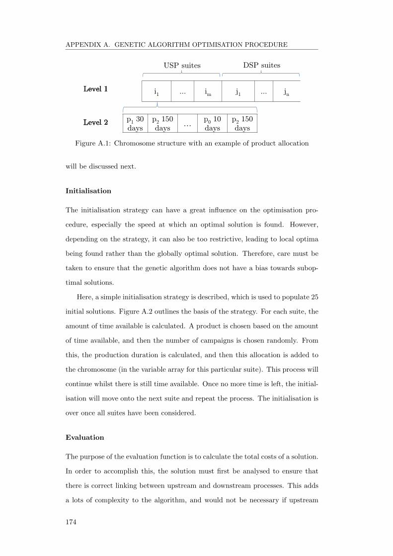
APPENDIX A. GENETIC ALGORITHM OPTIMISATION PROCEDURE
i1 ... im j1 ... jn
USP suites DSP suites
p1 30
days
p2 150
days…
p0 10
days
p2 150
days
Level 1
Level 2
Figure A.1: Chromosome structure with an example of product allocation
will be discussed next.
Initialisation
The initialisation strategy can have a great influence on the optimisation pro-
cedure, especially the speed at which an optimal solution is found. However,
depending on the strategy, it can also be too restrictive, leading to local optima
being found rather than the globally optimal solution. Therefore, care must be
taken to ensure that the genetic algorithm does not have a bias towards subop-
timal solutions.
Here, a simple initialisation strategy is described, which is used to populate 25
initial solutions. Figure A.2 outlines the basis of the strategy. For each suite, the
amount of time available is calculated. A product is chosen based on the amount
of time available, and then the number of campaigns is chosen randomly. From
this, the production duration is calculated, and then this allocation is added to
the chromosome (in the variable array for this particular suite). This process will
continue whilst there is still time available. Once no more time is left, the initial-
isation will move onto the next suite and repeat the process. The initialisation is
over once all suites have been considered.
Evaluation
The purpose of the evaluation function is to calculate the total costs of a solution.
In order to accomplish this, the solution must first be analysed to ensure that
there is correct linking between upstream and downstream processes. This adds
a lots of complexity to the algorithm, and would not be necessary if upstream
174

APPENDIX A. GENETIC ALGORITHM OPTIMISATION PROCEDURE
i = 1
tavailable ← maximum numberof days being scheduled
P ← set of products whichcan be produced in tavailable
p← random product from(P− previous product
chosen)
N ← maximum number ofcampaigns of p capable ofbeing produced in tavailable
n← random integer from 1to N , represents number of
campaigns chosen
Duration ← n× campaignduration
tavailable ← tavailable−duration
Add (p, duration) to suite’ssolution in chromosome
tavailable > 0?
i← i+ 1
i > numberof suites?
Finish
yes
no
no
yes
Figure A.2: Initialisation strategy
175
APPENDIX A. GENETIC ALGORITHM OPTIMISATION PROCEDURE
and downstream processes were modelled as one black-box process. These checks
must be carried out either in the evaluation function, or in both the initialisation
function and mutation operator.
Algorithm 1 shows the part of the evaluation function which deals with en-
suring enough material is available in USP suites before being purified for down-
stream production. It first goes through each USP suite and calculates inventory
levels for each product. Then, for every batch that is allocated in a DSP suite,
it first checks that there is available USP material, and then adjusts USP inven-
tory levels accordingly. Once all DSP batches have been accounted for, the USP
inventory costs can be calculated. Demands are met via a similar process but
for DSP inventory levels. Finally, the total cost is updated with the variable,
inventory and backlog costs.
Since both the intermediate product and final product have shelf-lives, the
material taken from the USP or DSP suites is always taken from the earliest pos-
sible time. Although not shown in Algorithm 1, when material from a USP suite
is required, a transfer matrix for that particular DSP suite is used to determine
the order that the USP suites should be analysed. This matrix is created when
the framework begins, and uses lexicographic analysis to determine for every DSP
suite which order of USP suites (based on transportation cost and time) material
should be sourced from.
Mutation operator
The mutation operator is shown in Algorithm 2, and is simply a modification
of the initialisation strategy. Instead of tavailable being the total available time
for the planning horizon, here it is equal to the time that was allocated to the
mutated product. In addition, the previous product is not excluded from the
set of products that can be chosen. In this way, production durations of existing
allocations can be extended. Finally, the solution is reduced such that allocations
of the same product are combined into one allocation, thereby reducing the size
of the variable array.
176

APPENDIX A. GENETIC ALGORITHM OPTIMISATION PROCEDURE
Algorithm 1 Extract of evaluation strategy
for each USP suite i dofor each product allocated to i do
Calculate when the batches are produced (considering ramp-up times)Calculate variable costCalculate inventory levels (daily)
end forend for
for each DSP suite j dofor each product allocated to j do
Calculate when the batches are producedrequiredAmount ← batchLoadday ← max(current day − USP shelf life, 1)while day ≤ current day and requiredAmount > 0 do
for each USP suite in transfer matrix dox← Take as much material as possible (up to requiredAmount)requiredAmount ← requiredAmount − xAdjust USP suite’s inventory for this and every subsequent dayif requiredAmount = 0 then
breakend if
end forif requiredAmount > 0 then
No DSP batches are produced at this timeReinstate any inventory that was subtracted from USP suites
end ifday ← day + 1
end whileCalculate inventory levels (daily)Calculate variable cost
end forend for
for each USP suite i doCalculate inventory cost for each product
end for
for each product dofor each demand do
requiredAmount ← demandday ← max(demand due date − DSP shelf life, 1)while day ≤ current day and requiredAmount > 0 do
for each DSP suite dox← Take as much material as possible (up to requiredAmount)requiredAmount ← requiredAmount − xAdjust DSP suite’s inventory for this and every subsequent dayif requiredAmount = 0 then
breakend if
end forday ← day + 1
end whileend fordemandPenalty ← requiredAmount × penalty
end for
for each DSP suite j doCalculate inventory cost for each product
end for
Cost ← variable costs + inventory costs + demand penalty costs
177

APPENDIX A. GENETIC ALGORITHM OPTIMISATION PROCEDURE
Algorithm 2 Mutation strategy
for each product allocation in chromosome doif mutate {based on probability, i.e. 20% chance of mutation} then
Do as per initialisation strategy, except:tavailable = time allocated to current productP does not exclude previous product
Reduce new products {p1 150 days followed by p1 150 days = p1 300 days}end if
end for
Results
The computational results of a one year capacity plan are shown in Figure A.3.
The number of evaluations run was 1000, and the total number of runs was 10.
The average fitness (which in this case is the total cost) across all 10 runs at
each evaluation is shown by a blue line. The range of values across the 10 runs is
shown by the grey area. The best solution obtained and the total time required
to run 1000 evaluations for 10 runs are also shown under the legend.
Two initialisation strategies were investigated, the first used the strategy
shown in Figure A.2, whereas the second initialisation strategy applied checks
on USP material prior to allocating DSP batches. That is, where as before the
checks were made in the evaluation function, in the second strategy the checks
were made in the initialisation and mutation functions. This led to a much nar-
rower range, resulting in a lower average fitness value. However, the increased
complexity of checking for USP material at each stage in the mutation operation
led to an increase in computational time, and there was no improvement in the
best fitness value obtained. For comparison, the one year capacity plan was also
optimised via the STN mathematical model described in Chapter 4. The optimal
solution was found to be 212.53, and this was obtained within 0.5 seconds.
Figure A.4 shows the comparison between the two initialisation/mutation
strategies on two year capacity plans. Again, the range is tighter for the strategy
which checks USP material inside the initialisation and mutation functions. How-
ever, the computational time has increased by more than four times, and the best
solution found was much inferior to the simple strategy. So the results suggest
that have a tighter range is not necessarily an important factor here, and does
178
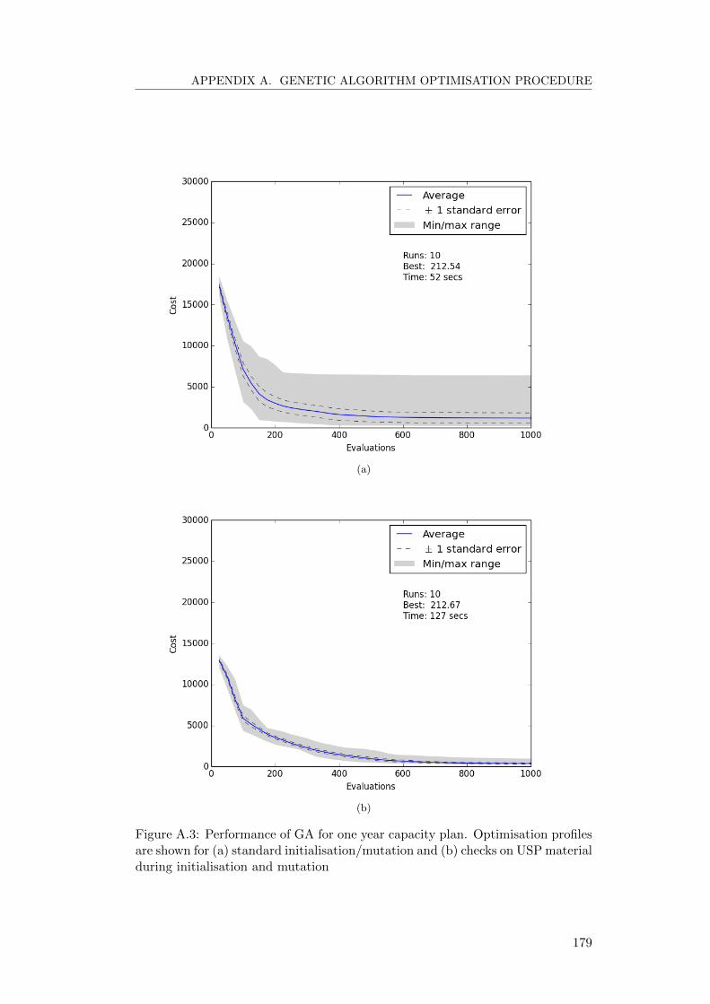
APPENDIX A. GENETIC ALGORITHM OPTIMISATION PROCEDURE
(a)
(b)
Figure A.3: Performance of GA for one year capacity plan. Optimisation profilesare shown for (a) standard initialisation/mutation and (b) checks on USP materialduring initialisation and mutation
179

APPENDIX A. GENETIC ALGORITHM OPTIMISATION PROCEDURE
not aid in performance or solution quality as may initially be presumed. Again,
the two year capacity plan was also optimised using a mathematical model. The
best solution found was 671.91, and was obtained in 5 seconds.
Both the one and two year capacity plans were much quicker to solve us-
ing mathematical techniques rather than the genetic algorithm implementation
shown here. Many improvements could be made to the initialisation and mutation
algorithms, but the main issue is that the way the chromosome is structured re-
stricts scalability. As the problem becomes larger and more years are planned for,
the size of the variable length arrays become ever greater, and any loops within
the mutation operation have a much larger impact on performance. Heuristics
and tweaks to the mutation and initialisation algorithms may also lead to local
optima, as was the case in Figure A.4b, where the best solution was not as good
as the simpler initialisation/mutation strategy.
In theory, the GA model described here should be able to obtain better solu-
tions than a discrete MILP model, simply because using a daily resolution allows
for more manufacturing flexibility. Owing to performance issues, however, longer
capacity plans (where this may be more noticeable) were not obtainable. Further
work must be conducted to investigate whether using a genetic algorithm for this
type of problem is of benefit, both in terms of solution quality and performance.
The results obtained so far suggest that mathematical techniques are a better ap-
proach. It seems that if genetic algorithms are to be used, a different chromosome
structure may be required, so that performance is not a limiting factor.
180

APPENDIX A. GENETIC ALGORITHM OPTIMISATION PROCEDURE
(a)
(b)
Figure A.4: Performance of GA for two year capacity plan. Optimisation profilesare shown for (a) standard initialisation/mutation and (b) checks on USP materialduring initialisation and mutation
181

APPENDIX A. GENETIC ALGORITHM OPTIMISATION PROCEDURE
182

Appendix B
Papers by the author
The following are papers that have been published by the author:
Siganporia, C., Ghosh, S., Daszkowski, T., Papageorgiou, L. G., and Farid, S. S.
(2012). Production planning of batch and semi-continuous bioprocesses across
multiple biopharmaceutical facilities. In Bogle, I. D. L. and Fairweather, M., edi-
tors, 22nd European Symposium on Computer Aided Process Engineering, volume
30 of Computer Aided Chemical Engineering, pages 377-381. Elsevier.
Siganporia, C. C., Ghosh, S., Daszkowski, T., Papageorgiou, L. G., and Farid, S.
S. (2014). Capacity planning for batch and perfusion bioprocesses across multiple
biopharmaceutical facilities. Biotechnology Progress, 30(3):594-606.
183