Seediscussions,stats,andauthorprofilesforthispublicationat:https://www.researchgate.net/publication/232562538

Straighttalkaboutlinearseparability

ArticleinJournalofExperimentalPsychologyLearningMemoryandCognition·May1997

DOI:10.1037/0278-7393.23.3.659

CITATIONS

105

READS

81

3authors,including:

JohnPaulMinda

TheUniversityofWesternOntario

35PUBLICATIONS1,168CITATIONS

SEEPROFILE

AllcontentfollowingthispagewasuploadedbyJohnPaulMindaon07June2014.

Theuserhasrequestedenhancementofthedownloadedfile.Allin-textreferencesunderlinedinblueareaddedtotheoriginaldocument

andarelinkedtopublicationsonResearchGate,lettingyouaccessandreadthemimmediately.

Journal of Experimental Psychology:Learning, Memory, and Cognition1997, Vol. 23, No. 3, 659-680

Copyright 1997 by the American Psychological Association, Inc.0278-7393/97/$3.00

Straight Talk About Linear Separability

J. David SmithState University of New York at Buffalo

Morgan J. Murray, Jr.New School for Social Research

John Paul MindaState University of New York at Buffalo

It is intuitive that prototypes and additive similarity calculations might underlie humancategorization, promoting a special appreciation of linearly separable categories. The failure todocument empirically this appreciation has helped focus interest instead on exemplarstrategies, multiplicative similarity calculations, and theory-based categorization. However,existing studies have mainly sampled poorly differentiated categories with small exemplarsets. Therefore, the present research repeated existing studies on linear separability, usingbetter differentiated categories better stocked with exemplars. Both the data patterns andmodeling suggest that prototypes and a linear separability constraint may have a strongerinfluence on categorization for these alternative category structures. The information-processing basis for this result is discussed.

Prototypes, Additive Evidence Rules, and the LinearSeparability Constraint

A basic cognitive task is to group objects (foods, preda-tors, mates) into psychological equivalence classes, allow-ing their similar treatment. An intuitive view of this processis that category members share a family resemblancegrounded in common features. According to prototypetheories, for example, category members are similar forbeing variations on a central tendency that participants learnand use in categorization. A generalized prototype principlelong anchored the literature on categorization (Homa, Rhoads,& Chambliss, 1979; Homa, Sterling, & Trepel, 1981; Mervis& Rosen, 1981; Posner & Keele, 1968, 1970; Rosch, 1973,1975; Rosch & Mervis, 1975; Smith, Shoben, & Rips, 1974).

To use a prototype, the categorizer could determine thefeatures a token shares with it and ask whether the combinedevidence (similarity) meets some criterion for inclusion inthe category. Typical category members would meet thiscriterion more quickly than atypical category members,producing the well-known typicality effects. Atypical cat-egory members could even persistently be categorized intoan opposing category if they resembled the opposingprototype.

Categories organized around a prototype will tend tooccupy a discrete and coherent region of multidimensionalstimulus space, a region that is partitionable away from

J. David Smith, Department of Psychology and Center forCognitive Science, State University of New York at Buffalo;Morgan J. Murray, Jr., Graduate Faculty, New School for SocialResearch; John Paul Minda, Department of Psychology, StateUniversity of New York at Buffalo,

Correspondence concerning this article should be addressed to J.David Smith, Department of Psychology and Center for CognitiveScience, Park Hall, State University of New York at Buffalo,Buffalo, New York 14260. Electronic mail may be sent via Internetto psysmith@acsu.buffalo.edu.

opposing categories. This coherence can be illustrated byusing the stimulus space in Figure I A. Suppose the lower-left stimuli and the upper-right stimuli are partitioned intocategories (Figure IB). Though neither size nor brightness isdiagnostic of category membership, the observer can stillcombine these independent sources of information, and,using this additive evidence rule, differentiate successfullythe larger-darker and smaller-lighter stimuli. In contrast,suppose one category includes the bottom-left and top-rightstimuli, whereas the other category includes the top-leftstimuli and bottom-right stimuli (Figure 1C). This partitionwould be difficult to learn using prototypes, because thestimuli do not occupy separable and coherent regions of thestimulus space, and because the prototypes (the categories'central tendencies) are coincident in the space.

Therefore, if prototypes and additive evidence rules doguide human categorization, then category learners willappreciate coherent and separable exemplar pools in stimu-lus space and may assume that categories are organized inthis way. In turn this might constrain the kinds of categoriesthey find natural to learn. Formally, this constraint wouldimply that humans prefer categories that are linearly sepa-rable or separable by a linear discriminant function (Medin& Schaffer, 1978; Sebestyen, 1962). Linearly separablecategories (Figure IB) are those that can be partitioned onthe basis of a weighted, additive combination of componentinformation. The geometric sense of this additive evidencerule is that a line through the two-dimensional stimulusspace cleanly separates the two exemplar sets. In contrast,the categories of Figure 1C are not linearly separable. Thereis no way to combine the independent information from sizeand brightness to unambiguously categorize the stimuli, andthere is no line that cleanly separates the exemplar sets.

Isn't it plain that the absence of differentiable prototypesand coherent, separable exemplar pools will defeat learningin the stimulus partition of Figure 1C? After all, in this

659

660 SMITH, MURRAY, AND MINDA

A. Stimulus Space

B. LS Partition

C. NLS Partition

Figure 1. A size and brightness stimulus space (A) partitionedinto categories that are linearly separable (B) or not (C). LS =linearly separable; NLS = nonlinearly separable.

example the two categories are not well differentiated bybasic perceptual similarity. Actually, participants mighttranscend this difficulty in a variety of ways. They mightpossess exemplar-based strategies powerful enough to labelcorrectly the stimuli even though they are "disorganized" inmultidimensional space. They might code the stimuli morerelationally and as conftgural wholes and note which wholeconstellations of features deserve which category labels.They might note conceptually that positively correlated sizeand darkness occupy one category, and negatively correlatedsize and darkness the other.

These possibilities have been an integral part of the recentcategorization literature—for sound empirical reasons (Malt& Smith, 1984; McKinley & Nosofsky, 1995; Medin,Altom, Edelson, & Freko, 1982; Medin & Schaffer, 1978;Medin & Schwanenaugel, 1981; Murphy & Medin, 1985;Nosofsky, 1986, 1987). In fact, participants are capable oflearning NLS categories of the kind shown in Figure 1C(Nosofsky, 1987)—they show no evidence of a linearseparability constraint that makes only linearly separable(LS) category structures natural and leamable. Lingle,Altom, and Medin (1983, pp. 93-94) even argued that thestructures of Figures IB and 1C might be learned equallyeasily by a participant who coded stimulus dimensionsrelationally. Stopping short of this strong claim, an impor-tant question remains as to whether, and when, linearseparability constrains human categorization (Ashby &Gott, 1988; McKinley & Nosofsky, 1995).

Evaluating the Linear Separability Constraint

Exploring this question, Medin and Schwanenflugel (1981)noted the dominance of prototype models and additiveevidence rules in the literature, the theoretical importance ofan LS constraint if it did actually limit the range of naturaland learnable category structures, and a surprising empiricalsilence on this issue. Accordingly, they asked whethernonlinearly separable (NLS) categories were unnatural andpoorly learnable for participants. In fact, they asked thequestion elegantly, for they matched the LS and NLScategories for their within- and between-category similari-ties (assuming equal salience across dimensions). In con-trast, linear separability and stronger similarity relationswere confounded in the stimulus sets of Figure 1.

Figure 2 (A-C) shows the structure of three-dimensionalLS and NLS categories used by Medin and Schwanenflugel(1981, Experiment 4). The category structures have similardistributions of features with values of one and zero favoringCategories A and B, respectively, always for two of threeexemplars in a category. In the LS case, each exemplar hastwo of three features in common with the category proto-types: 111 and 000. Thus all items can successfully beclassified by using an additive evidence rule that compareseach token to the prototypes and looks for an evidence scoreof 2.0. Figure 2-C shows the stimulus space for thesecategories. One can easily imagine the plane (three minusone dimensions) that partitions the cube (three dimensions)and separates the As and the Bs. These categories areplanarly (linearly) separable.

In the NLS case an additive evidence rule will not suffice.For one thing, it will produce categorization errors forStimuli Al and B3, which have more features in commonwith the opposing prototype. For another thing, the NLScategories contain category members that are complementsof one another because they have no common features (i.e.,Al and A2 and B2 and B3). These stimulus pairs rule outsuccessful categorization using any linear discriminant func-tion. That is, any weighting of the three independent cuesthat allows the successful classification of Stimulus Al (e.g.,a very heavy weighting on the first feature) will ensure themisclassification of Stimulus A2. Figure 2C shows that thesecomplementary stimuli are maximally distant in the stimulusspace. These categories are not planarly (linearly) separable,for no plane could ever partition the stimulus space andseparate the As and Bs.

These two aspects of NLS category structures—exceptionitems and complementary stimulus pairs—are connected. Tothe extent that one of the complementary stimuli belongswith its category mates (e.g., A2 with A3), the other memberof the complementary pair will tend to be an outlier, anexception to the category, and it will seem in an intuitiveprototype sense to be "trying to belong" to the opposingcategory (e.g., Al). If one member of the complementarypair is really prototypical in the category, its complementwill be really exceptional in the category.

If humans rigidly depend on prototypes in categorization,then NLS categories might be unlearnable. The exception

LINEAR SEPARABILITY 661

A. LS CategoriesA B

011 100

110 001

101 010

B. NLS Categories

A B

100 000

011 001

111 110

C. Three-dimensionalstimulus space

0 1 0

0 0 0

0 1 1

0 0 1

1 1 0

TOO

01

D. Performance

<Q 1 0 - ,33 9"

z 7-

h 4-

< o

Exception

Normal

1 2Experiment

Figure 2. LS (A) and NLS (B) categories used in Experiment 4 of Medin and Schwanenflugel(1981). (C) The stimulus space of those categories. (D) Performance on normal and exception itemsin three NLS category tasks (on the horizontal axis: 1 refers to Medin & Schaffer, 1978, Experiment1, Stimulus 15 vs. all others; 2 refers to Medin & Schwanenflugel, Experiment 1, NLS Stimulus Alvs. seven others; and 3 refers to Medin & Schwanenflugel, Experiment 2, NLS Stimuli Al and B3vs. six others, generalizations condition). LS = linearly separable; NLS = nonlinearly separable.

items, too similar to the opposing prototype, might lastinglybe categorized incorrectly, yielding below-chance perfor-mance on them. The complementary pairs of items mightlastingly be wrongly placed into opposing categories. Dis-cussing this linear separability constraint, Wattenmaker,Dewey, Murphy, and Medin (1986) stressed that categoriesmust be linearly separable "for a prototype process to workin the sense of accepting all members and rejecting allnonmembers" (p. 160). In fact, any categorization processbased on a weighted function of independent propertiesimplies that NLS categories should produce an indefinitelylong struggle with exception items (Wattenmaker et al., 1986).

Yet research has not documented this struggle. Medin andcoworkers found that the errors made on exception itemswere only slightly greater than the errors made on normalcategory members (Figure 2D), and performance on excep-tions was better than chance, not below chance as if thestimuli had been assimilated to the opposing prototype.

Participants were not just slavishly using a prototypestrategy. Instead, they may have been processing wholefeatural complexes relationally or memorizing individu-ated exemplars.

This flexibility in processing NLS categories has helpeddiscourage categorization models that emphasize the summedevidence provided by separable and independent perceptualcues and has encouraged an important shift in categorizationtheory and research. Now the emphasis is on exemplar-based models of categorization, multiplicative calculationsof similarity, and conceptually based categories. This shift isimportant, given a centuries-old conviction by philosophersand psychologists that prototypes and additive evidencerules do matter (e.g., Locke, 1690/1959). The purpose of ourarticle is to encourage more research on when these differentcategorization strategies will appear and when differentcategorization models will be appropriate. The existing researchon NLS categories has only filled in part of the picture.

662 SMITH, MURRAY, AND MJNDA

Interpretative Limits on Existing Research

Small Exemplar Sets

McKinley and Nosofsky (1995) noted that existing re-search has mainly featured small exemplar pools (about fouritems per category), whereas prototypes and a linear separa-bility constraint might emerge only for large exemplar pools.In fact, Medin and Schwanenflugel (1981) and Medin,Dewey, and Murphy (1983) worried that their small catego-ries would encourage a paired-associate learning strategywherein the LS constraint could not show because therewere only a few stimulus-category pairings to be learned.Therefore, in additional experiments they included manyspecific tokens of the few logical types in each category.They still found evidence for exemplar-based strategies andstill found no constraint favoring the learning of LS catego-ries. Unfortunately, though, these experiments raised twoproblematic issues. First, if participants considered thestimuli as abstract types, varying along four dimensions, theeffective exemplar pools would still be only about four percategory, and not the number of specific tokens (e.g., withdifferent instantiations of blonde hair or shirt color). Second,these categories were difficult for participants to learn—38%, 66%, or 72% of participants failed to reach even amodest learning criterion (Medin et ah, 1983, last-name-infinite condition; Medin & Schwanenflugel, 1981, Experi-ments 3 and 4).

Learning Difficulties

In studies beyond those just mentioned, 30%, 40%, or60% of participants failed ever to meet the preset learningcriterion (four experiments in Medin & Schaffer, 1978;Medin & Schwanenflugel, 1981; Medin & Smith, 1981). Incontrast, participants in other studies have met a criterion of36 errorless trials (Hartley & Homa, 1981), 70 trials (Homaet al., 1981), or even 90 trials (Homa et al., 1979). Byanother measure, participants in the existing experimentshave an asymptotic performance of about 80%, even afterreceiving 108-288 potential training trials (Medin & Schaf-fer, 1978, Experiment 2; Medin & Schwanenflugel, 1981,Experiment 3). In contrast, Kemler Nelson (1984) and Smithand Shapiro (1989) used categories that let participantsexceed 90% accuracy with only 24 training trials. In Homaet al. (1979) and Hartley and Homa (1981) participantsachieved almost perfect learning. Indeed participants oftenexceed 80% correct after a week's delay, when given only 6s to study the eight stimuli in two categories, or underincidental conditions (Hartley & Homa, 1981; Homa et al.,1979; Homa et al., 1981; Kemler Nelson, 1984; Smith &Shapiro, 1989). Thus, research must still document thecharacter of categorization strategies when the categories are"easier" to learn.

Impoverished Category Structure

Existing LS-NLS comparisons have typically featuredimpoverished category structures. Structural ratio, whichcan be defined as the ratio of the similarity of exemplars

within categories to the similarity of exemplars betweencategories, is a useful way to demonstrate this fact aboutexisting LS-NLS comparisons (see also Homa et al., 1979,pp. 13-14). Figure 3A shows a space containing 700hypothetical category structures. The stimuli for thesecategories were constructed by using six binary dimensions.There were seven exemplars in each category, derived fromthe prototypes 0 0 0 0 0 0 and 1 1 1 1 1 1 for the twocategories. To make this figure, the 42 stimuli that had threeor more features in common with a prototype were dividedinto three classes: Class 1 (those with six or five commonfeatures), Class 2 (those with four common features), andClass 3 (those with three common features). Then 35selection procedures were generated as follows: 6 1 0,6 0 1,5 2 0, 5 1 1, 5 0 2 , . . . 0 0 7. Thus, the first 20 stimulus setscontained, in each category, 6 Class 1 stimuli and 1 Class 2stimulus. The last set of 20 stimulus sets contained 7 Class 3stimuli in each category. All repeats of items between orwithin categories were ruled out. To be fair to the twoinfluential ideas about similarity calculations, the index ofcategory structure has been calculated by using both additiveand multiplicative similarity rules. The correlation betweenthe two indices was .97, making the kind of similaritycalculation one adopts for the present purpose a matterof indifference.

Figure 3B shows in the same space the 12 categorystructures that have been used for six existing comparisonsbetween LS and NLS categories. These comparisons can befound in Medin and Schwanenflugel (1981, Experiments1-4), Kemler Nelson (1984, Experiment 3), and Watten-maker et al. (1986, Experiment 1). There appear to be fewerthan 12 data points because some category structures havebeen repeated. All of these comparisons have used poorlydifferentiated categories by either metric. This is a naturaloutcome of the careful stimulus control these experimentsrequire. Yet this poor differentiation means that existingcategory structures contain highly similar exemplars thatparticipants are very likely to confuse; indeed this hasseemed a virtue of the experiments (Medin & Schwanenflu-gel, 1981, p. 361). Sometimes there are more close matchesbetween exemplars across categories than within categories(Medin & Schwanenflugel, 1981, p. 358). Also in thesecategories, the prototypes hardly stand out as special, evenwhen they are presented, and individual features are poorlypredictive of category membership (50%-75%). Possiblythese "categorization" tasks sometimes degenerate intoidentification tasks, in which participants rotely associatewhole instances and their labels but have no sense oforganized categories as they apply the labels. Medin andSchwanenflugel (1981, p. 365) entertained just this worryabout their specialized categorization tasks. Though humansmay depend on exemplar encoding, not prototypes andlinear separability, given impoverished category structure, itis still possible that prototypes and linear separabilitybecome important given well-differentiated categories (Me-din & Schwanenflugel, 1981; Medin & Smith, 1981, pp.171-172). (One can explore more fully the possible relationsbetween exemplar memorization and categorization inShepard, Hovland, & Jenkins, 1961; Medin & Schwanen-

LINEAR SEPARABILITY

B.

663

1.25 1-5 1.75 2 2.25 2.5 2.75Structural Ratio (AddWra)

3-

1 1.25 1.5 1.75 2 225 2.5 2.75Structural Ratio (Addfflv»)

D.

00-,

80-

70-

50-

40-

30-

20-

10-

o

g • «

•• Prototype Modrt

O Context Model

1

1.25 1.5 1.75 2 2£5 2.5 2.75Structural Ratio (Additive)

I-,

g0.9-= 0.8-

So.7-

f 0.4-O0.3-C0.2-

fio.1-0-

*O

• Prototype Mo (M

O ContaxtMotM

1.25 1.5 1.75 2 2.25 2.5 2.75Structural Ratio (Additive)

Figure 3. (A) Seven hundred hypothetical category structures illustrating the range of categorydifferentiation that is easily available. (B) The level of category differentiation provided in sixexisting comparisons between linearly separable and nonlinearly separable categories. (C) The fit oftwo categorization models to humans' performance when they are given categories of differentstructural ratios (see Nosofsky, 1987). (D) The fit of two categorization models to humans*performance when they are given categories of different structural ratios (see Medin & Schaffer,1978; Medin & Smith, 1981).

flugel, 1981, pp. 361-362; Nosofsky, 1984,1986,1987; andSmith, 1989.)

Category Differentiation and the Fit of Models

Some evidence hints at a link between good categorystructure and the use of prototypes in categorization. Forexample, Nosofsky (1987) gave his participants six differentcategory structures, which varied in structural ratio from1.17 to 2.39, calculated by comparing the average Euclideandistance among stimuli between categories and withincategories. Nosofsky fit a prototype model and an influentialexemplar-based alternative to participants' performance witheach stimulus set. Where categories are well differentiated,the models perform equally. For poorly differentiated catego-ries, prototype models do not suit at all (Figure 3C).

Medin and Schaffer (1978) and Medin and Smith (1981)also fit exemplar-based and prototype-based models tocategorization performance (Figure 3D). In conditions of

low-to-moderate category structure (structural ratio — 1.46),both models performed equivalently when different indicesof observed and predicted performance were correlated. Onecondition had weaker category structure (structural ra-tio - 1.28), and it produced the one decisive failure of theprototype model. Apparently, the prototype model gainsrapidly over structural ratios of 1.2 to 1.5, for two- orfour-dimensional stimulus sets, integral or separable dimen-sions, and continuously varying or binary dimensions.

There are a variety of possible perspectives on thesegraphs. One can point to the exemplar model's advantage forpoorly structured categories, or one can worry that thatmodel fits best only when prototype strategies are under-mined and exemplar strategies are mandatory. One can notethe exemplar model's greater staying power, for it handles"bad" and "good" category structures, or one can note thatprototype models achieve parity just where they should andonly where they could—where robust, differentiable proto-

664 SMITH, MURRAY, AND MINDA

types are on the scene. Or, one can downplay both good fitsfor well-differentiated categories because formally the mod-els must fit well and must start to converge for thehomogeneously excellent performances supported by higherlevels of category structure and predicted by both models.

Ideally, though, the question could be a psychologicalone, not a formal one. Figures 3C and 3D suggest thepossibility of an interesting psychological transition thatoccurs as structural ratio improves, gradually suggestingprototype strategies, and gradually making them useful. Ofcourse it will require diagnostic category structures to showthis transition if it exists. Then one may be able to tell whatstrategies emerge for different kinds of categories and whatmodels are appropriate for describing different perfor-mances. In our view, this remains an important unknown inthe existing literature.

Experiment 1

Existing research on NLS categories has sampled anexemplar-poor, poorly differentiated, and poorly learnableregion of the universe of category structures. Consequently,the inference remains only specific and limited that humansuse exemplar-based strategies and are free from a constraintfavoring linear separability. Accordingly, in Experiment 1we duplicated existing comparisons between LS and NLScategories, using better differentiated, more exemplar-richcategories. We explored the possibility that these alternativecategory structures will encourage the use of prototypestrategies and will subject categorizers to a linear separabil-ity constraint.

Method

Participants. Sixty-four members of a university communitywere paid to participate in this study.

Stimuli and category structures. The crucial aspect of thedesign was to use six-dimensional stimuli instead of the usual threeor four dimensions. This allowed larger exemplar pools and betterdifferentiated categories than were previously used.

The stimuli were pronounceable six-letter nonsense words withthe following pattern of consonants (Cs) and vowels (Vs): CVCVCV(see also Smith & Shapiro, 1989; Smith, Tracy, & Murray, 1993;Whitllesea, 1987; Whittlesea, Brooks, & Westcott, 1994). Stimulusgeneration began with the creation of two prototype pairs (bunoli-kypera and girupo-4etany). The first and second members of eachpair were designated as stimuli 0 0 0 0 0 0 and 1 1 1 1 1 1 ,respectively. These prototypes were created randomly but withseveral constraints to ensure the pronounceability of all stimuli, theorthographic appropriateness of all stimuli, the identical syllabifica-tion of all stimuli, and the roughly equal use of all vowels. Forexample, q (which is followed by two vowels), c (which changessounds depending on the vowel following), and e in final position(which often changes syllabification) were disallowed. Each proto-type pair contained six different vowels and six different consonants.

The Appendix (top) shows the structure of the LS and NLSstimulus sets with poorer category structure that should presentmore performance difficulties. Each LS category contained sevenstimuli that shared four features with the category prototype. Therewere no exception items. A prototype strategy, using an additiverule that summed across independent attributes, would allow

perfect categorization. Each NLS category contained three stimuliwith five typical features, three stimuli with four typical features,and one exception that had five atypical features. The similarityrelations in the NLS categories were heterogeneous, but the clusterof highly similar instances combined with the exceptions balancedoverall similarity at the level for the LS categories. The comple-ment of the exception also appeared (Stimuli A2 and A7 andStimuli B3 and B7), ruling out an additive categorization rule andguaranteeing NLS categories.

These general category structures were predetermined to allowthe generation of well-matched LS and NLS stimulus sets. Afterthese assignments, hundreds of possible stimulus sets were com-puter generated and screened for LS and NLS category structuresthat matched in several ways. The two stimulus sets had identicalexemplar-exemplar similarity, both within category (an average of3.47 shared features) and between category (2.69 shared features),and identical exemplar-prototype similarity, both within category(4.00 features) and across category (2.00 features). By eitherstandard, the two stimulus sets had identical structural ratios (1.29when the exemplar-exemplar similarities were used) and structuralratios like those in previous LS-NLS comparisons. These calcula-tions assumed additive similarity calculations and equal saliencefor all of the features.

In addition, the LS and NLS stimulus sets were matched in theoverall informativeness of all attributes. For the LS categories,Group A stimuli took the typical value—zero—four, five, four, six,five, and four times for attributes 1-6, and Group B stimuli took thetypical value—one—four, four, six, five, four, and five times forattributes 1-6. These numbers were identical for the NLS catego-ries. Thus, there were no criteria! attributes at work in thesestimulus sets, and any single-letter strategy should have beenidentically salient and viable in both stimulus sets.

TTie category structures were not matched, however, if oneconsiders the number of highly similar pairs of exemplars. NeitherLS category had any highly similar exemplar pairs (e.g., five sharedfeatures), the NLS categories featured seven pairs. As Medin andothers have noted, this might grant the NLS categories a learningadvantage if exemplar-based strategies dominated categorizationand highly similar pairs of exemplars retrieve each other and affordeasy categorization.

The six dimensions of the stimulus array were further exploitedto create matched LS and NLS category structures with betterdifferentiated categories that participants might find easier to learn.The structure of these LS and NLS categories is also shown in theAppendix. The LS categories contained one prototype, two stimuliwith five typical features, and four stimuli with four typicalfeatures. There were no exception items; an additive rule wouldcorrectly categorize all stimuli. Again the LS similarity relation-ships were fairly homogeneous but weakened compared with thecluster of highly similar exemplars in the matched NLS categories.

The NLS categories contained one prototype, five stimuli withfive features in common with the prototype, and one exception itemthat shared five features in common with the opposing prototype.The cluster of highly similar instances combined with the excep-tion item balanced overall similarity at me level for the LS task.The complement of the exception stimuli also appeared (StimuliA5 and A7 and B5 and B7), also ruling out an additive decision rule.

These category structures allowed well-matched LS and NLSstimulus sets that were chosen from among hundreds of computer-generated sets. The two category structures had identical exemplar-exemplar similarity, both within category (3.88 features) andbetween category (2.12 features), and identical exemplar-prototype similarity, both within category (4.57 features) andbetween category (1.43 features). By either standard, the two

LINEAR SEPARABILITY 665

category structures had identical structural ratios (1.83 when theexemplar-exemplar similarities were used) and more categorystructure than the poorly differentiated stimulus sets.

In addition, LS and NLS categories were matched in the overallinformativeness of all attributes. For the LS categories, Group Astimuli took the typical value—zero—five, five, five, six, six, andfive times for attributes 1-6, and Group B stimuli took the typicalvalue—one—five, five, five, six, six, and five times for attributes1-6. These numbers were identical for the NLS categories. Againthere were no criteria! attributes available in either of thesestimulus sets, and any single-letter strategy should have beenidentically salient and viable in both of them.

The categories were not matched, however, if one considers thenumber of highly similar pairs of exemplars. Once again the NLScategories offered more highly similar exemplar pairs and mightsupport best exemplar-based strategies in categorization. Thiscould give the NLS categories a learning advantage if exemplar-based strategies dominated the processes of categorization.

For both the poorly structured and moderately structured catego-ries, two LS and two NLS tasks were constructed, one using eachprototype pair. Each task contained 196 trials (14 blocks) numberedconsecutively without visible breaks. Each block contained onerandomly generated run through the seven stimuli in each category.The stimuli were arranged into four random orders for differentgroups of participants.

Procedure. Participants revealed each successive trial througha window cut in white paper. This ensured trial-by-trial presenta-tion and prevented scanning forward and backward along the page.Participants classified each stimulus as an A or B on a separate,numbered answer sheet. The answer to each trial was printed belowit, invisible while the participant responded but available afterwardas feedback. Participants responded at their own pace—the ex-perimental session took approximately 1 hr. Participants wererandomly assigned to LS and NLS conditions and to the particularprototype pair and order of stimulus presentation they would receive.

The instructions for the categorization task were as follows:

In this experiment you will see nonsense words, each sixletters long, which can be classified as Group A or Group Bwords. Your task in this experiment is to look closely at eachword as it appears and figure out how you can tell whether theword belongs to Group A or Group B. At first the task will bequite difficult, but with time, and by studying the wordscarefully, you should be able to answer correctly.

The instructions included a description of how to use the paperwindow and how to reveal the correct answer to obtain feedback onone's performance. Participants were told to "study the word andthe answer together to try and gain more information about how thewords can be classified."

Results

These categories, even those with moderate categorystructure, were difficult to learn. Participants were 67%correct overall. Possibly the present manipulations to in-crease category structure still did not increase structural ratioenough to create easily learnable categories. After all,structural ratios of 1.83 are middling in comparison to thesweep of category structures shown in Figure 3A. Anotherpossibility is that the larger exemplar pools are underminingexemplar memorization, counteracting the benefits of in-creased structural ratio.

The data were analyzed by using a four-way analysis of

variance (ANOVA) with low-moderate structural ratio,LS-NLS, and Prototype 1-2 as between-subjects variablesand trial block as a within-subject variable. Two effects werereliable (Figure 4A). First, despite the difficulty of bothcategory structures, significant learning occurred across trialblocks, F(13,728) = 14.41, p < .05, MSE = 0.194. Second,performance was better for the categories with moderatestructural ratio, F(l, 56) = 13.28, p < .05, MSE = 1.819.Overall accuracy rates were 62% for the poorly structuredcategories and 71% for the moderately structured categories.This held for the LS categories considered alone (62% vs.68%) and for the NLS categories considered alone (62% vs.74%). Final accuracy rates were also higher for the moder-ately structured categories (70% vs. 80%). This result alsoheld for the LS categories (67% vs. 80%) and the NLScategories (72% vs. 79%). Moreover, 2 participants giventhe poorly structured categories achieved an errorless blockof 14 trials, compared with 8 participants given the moder-ately structured categories. The success of the manipulationto increase category differentiation reinforces the idea thatstructural ratio often predicts learnability in a categorizationtask—both prototype-based and exemplar-based models ofcategorization comfortably predict this result. A structuralratio of about 1.3, seen in previous LS-NLS comparisonsand in the present poorly differentiated category structures,often makes category learning very difficult.

A third effect did not obtain, there was no performanceadvantage for the LS categories over the NLS categories(Figure 4B). Performance was equivalent throughout learn-ing, F(l, 56) = 1.48, ns, MSE = 1.819. Thus, a constraintfavoring linear separability was not evident in overallpercentage correct.

However, overall performance is not generally suitablefor indicating such a constraint. The problem lies in thedifferent structure of LS and NLS categories. The NLScategories contain a cluster of similar items and oneexception item. To achieve equivalent category structureoverall, the homogeneous similarity relationships in the LScategories are deliberately weakened. Suppose that thisweakening creates performance on 14 LS items of 80%;whereas 12 normal NLS items are performed at 90%, and 2exception NLS items are performed at 20%. Overall perfor-mance is equated. Nonetheless, something has gone badlywrong in the NLS condition. Participants have failed to learnthe exception items and therefore have failed to learn theNLS categories in the sense of including category membersand excluding nonrnembers. One might rather say thatparticipants have insisted on reallocating the exceptionitems into the wrong categories and have constructed goodLS categories for themselves. In such a case, a strong linearseparability constraint would have been at work inparticipants' processing, but it would be invisible in over-all performance.

Constraint here simply means that participants' decisionboundaries are too rigidly "straight" to bend across thestimulus space and place the exception items in the correctcategories. The result is systematic errors on the exceptionitems, their effective reallocation into the opposing catego-ries, and the de facto construction of good LS categories by

666 SMITH, MURRAY, AND MINDA

B.

4 6 8 10 12 14TrW Block

L8

4 6 8 10 12 14Trial Block

D.

Normal

Exception

A A

0 2 4 6 8 10 12 14Trial Block

Exception

1 2 3 4 5Experiment

Figure 4. (A) Performance on the poorly and moderately differentiated categories by trial block inExperiment 1. (B) Performance on the linearly separable (LS) and nonlinearly separable (NLS)categories by trial block. (C) Performance on nonnal and exception items by trial block, for allparticipants in the moderately differentiated NLS condition. (D) Performance on normal andexception items in five NLS category tasks (on the horizontal axis: 1 refers to Medin & Schaffer,1978, Experiment 1, Stimulus 15 vs. all others; 2 refers to Medin & Schwanenflugel, Experiment 1,NLS Stimulus A1 vs. 7 others; 3 refers to Medin & Schwanenflugel, Experiment 2, NLS Stimuli A1and B3 vs. 6 others, generalizations condition; 4 refers to the poorly differentiated NLS condition ofExperiment 1; and 5 refers to the moderately differentiated NLS condition of Experiment 1).

participants. This constraint is not logically or necessarilylinked to any particular processing assumption. The facts ofsystematic errors, deallocation, and de facto LS categorieswould still be true, the LS constraint would still hold sway,whether participants were processing the stimuli usingprototypes, exemplars, rules, or anything else. However, theliterature has traditionally made a strong link between theLS constraint and prototype processing, to which we return(Lingle et al., 1984; Medin & Schwanenflugel, 1981;Murphy & Medin, 1985; Wattenmaker et al., 1986).

The LS constraint was operative in the present data,especially for the moderately differentiated NLS categories(Figure 4C). To assess this effect, we entered the NLS datainto a three-way ANOVA with exception-normal items andtrial block as within-subject variables and low-moderatestructural ratio as a between-subjects variable. The excep-tion items were performed much worse than the nonnal

items, F(l, 30) = 56.82, p < .05, MSE = 1.409. In fact, theexception items were performed far below chance, meaningthat despite feedback, participants consistently placed theexception items into the wrong category (z > 2.58, p < .05),even in the final block.

Moreover, performance had an opposite dynamic betweenthe normal and exception items. There was a significantinteraction in the ANOVA between low-moderate structuralratio and exception-normal item performance, F(l , 30) =5.74, p < .05, MSE = 1.409. From the poorly structured tothe moderately structured categories, participants becamemore accurate on the normal items (66% vs. 80%), but lessaccurate on the exception items (44% vs. 37%).

Recall that Figure 2D showed that the exception itemswere performed about the same as nonnal items in poorlydifferentiated category structures. Figure 4D includes thosethree studies in a broader perspective, including the results

LINEAR SEPARABILITY 667

from the present poorly structured and moderately structuredNLS categories. In the present case, with larger exemplarsets and better differentiated categories, performance be-comes far more heterogeneous because performance onnormal items and exception items diverges.

Of course, prototype models account easily for thisdivergence. Given assimilation to prototypes, participantsshould insist on forming good LS categories for themselvesand should show poor exception-item performance giventhis reorganization. In fact, this is just what Wattenmaker etal. (1986) predicted would occur when participants rigidlyapply prototype representations to NLS categories: Theyshould lastingly place exception items into the wrongcategories and thereby reassert the linear separability that aprototype strategy demands (Medin & Schwanenflugel,1981; Murphy & Medin, 1985). Thus the present resultscould suggest the interesting possibility that prototypestrategies are emerging given the category structures ofExperiment 1.

However, formal modeling offers a crucial additionalperspective on the NLS data pattern, for it is possible thatexemplar models might also predict this reallocation of theexception items and might also predict that participants willoperate under a linear separability constraint given thepresent category structures. We take this possibility seri-ously, despite the frequent claim in the literature thatexemplar processing is a primary strategy by which partici-pants can transcend the LS constraint enforced by prototypemodels (Lingle et al., 1984; Medin & Schwanenflugel, 1981;Wattenmaker et al., 1986). Accordingly, following Medinand coworkers, we contrasted an exemplar model featuringmultiplicative similarity calculations and a prototype modelfeaturing additive similarity calculations. The contrast be-tween these two models has been critical in many formalstudies of perceptual categorization. (We note that othermodels, such as exemplar models with additive similaritycalculations and prototype models with multiplicative simi-larity calculations, are logically possible and potentiallyinteresting too; see Nosofsky, 1992.)

In making the same contrast here, one interesting possibil-ity is that the prototype model might make a better showingin the category structures of Experiment 1 than it has inprevious comparisons involving exemplar-sparse, poorlydifferentiated categories. Another interesting possibility isthat the exemplar model might start to fail in fitting some ofthe participants1 data.

The Parity Between Models of Categorization

Procedure for fitting and testing models. In evaluatingthe exemplar model, we focus on the original context modelof Medin and Schaffer (1978), preserving the connection totheir work and the access to important intuitions. Nosofsky(1984, 1986; see also McKinley & Nosofsky, 1995) providedmore formal and general treatments of the context model.

In the exemplar model, the to-be-classified item in thepresent tasks would be compared with the seven A exem-

plars (including itself if it is an A), and with the seven Bexemplars (including itself if it is a B), yielding an overallsimilarity index of the item to Category A members andCategory B members. Dividing overall A similarity by thesum of overall A and B similarity would yield the probabilityof an A categorization. Crucially, each comparison betweena stored trace and the item would calculate similaritymultiplicatively. To use a simplified example, the trace andthe item would be compared along each of six dimensions,and the dimensional comparison would yield a 1.0 for amatching feature,. 1 for a mismatching salient feature, and .9for a mismatching nonsalient feature. The similarity be-tween the trace and the item would be the product of thesesix dimensional weights—1.0 for identity, but. 1 for a single,salient difference. One sees from this simple example thatsimilarity decays very rapidly in the exemplar model asfeatural dissimilarities accumulate; indeed, in some configu-rations (i.e., for some sets of similarity weights) the exem-plar model strongly emphasizes exact identity.

In fitting the exemplar model to target performances, wesampled 46,656 sets of weights in a grid search of theparameter space. Each dimensional weight was varied from.00 to 1.00 in .2 intervals, in nested fashion. For each set ofweights we calculated predicted categorization probabilitiesfor the 14 stimuli in a stimulus set, and we compared thesepredicted performances to the target performance. Themeasure of fit was the sum of the squared deviationsbetween observed and predicted performance, and in thecourse of a run that distance was minimized.

Extensive additional simulations confirmed that these gridsearches were finding nearly the best fits available in theparameter space. In these simulations, the parameter spacewas seeded with six different starting configurations (e.g.,the best parameters from the grid search, parameters indicat-ing completely divided attention, and parameters indicatingcomplete attention to one or two randomly chosen at-tributes), and a fine grained, hill-climbing algorithm soughtthe best fitting state from there. Subsequently, we took thebest fit achieved by any of the six hill climbs and subtractedthis from the fit achieved by the best node of the grid. Acrossthe 48 individual participants who are the primary focus ofthe modeling in this article, and who were modeled individu-ally with a grid search and with six hill-climbing seeds, theaverage improvement in fit was negligible—.006 for theprototype model and .006 for the exemplar model. Giventhat result, the grid searches have the virtue of beingcomprehensive and systematic without the need for specify-ing starting configurations that could favor one model overanother. In other cases, though, hill-climbing algorithmsmay be the preferred alternative.

To evaluate the prototype model, we supposed that eachto-be-categorized item would be compared with the categoryprototype along the six independent dimensions, usingadditive similarity calculations. Mismatching features con-tribute zero similarity, matching features contribute theamount of their dimension's weight. The six dimensionalweights have typically been required to sum to 1.0. In thesimplest case the prototype-item similarity is taken to be theprobability of a correct categorization, and its complement

668 SMITH, MURRAY, AND MINDA

the probability of an error. (The prototype's self-similarityis 1.0.)

As is customary, though, an additional free parameter wasadded to the prototype model because of the fixed sum of thedimensional weights. In our case, this additional guessingparameter captured participants' error proneness with thesedifficult category structures. Without the guessing param-eter, for example, the prototype (with perfect self-similarity)would always have perfect predicted performance. Thus itwas assumed that some proportion of the time G participantssimply guessed A or B haphazardly. On the other 1-Gproportion of trials with that stimulus the participants usedprototype similarity as already described (see also Medin &Smith, 1981).

To analyze the prototype model's behavior, a grid searchinstantiated all of the allowable configurations of the sixdimensional weights when they varied from 0 to 1.0 in .1increments. There were 3,003 configurations that preservedthe sum of 1.0. In association with a guessing parameter thatalso varied from 0 to 1.0, the grid search evaluated 33,033parameter settings. Once again the sum of the squareddeviations between observed and predicted categorizationperformance was minimized.

Extensive additional simulations investigated whethertending to one inequity (by giving the prototype model anequivalent number of free parameters) created anotherinequity (by not allowing the exemplar model to incorporateguessing). In these simulations, the parameter space wasagain seeded with six different starting configurations, and afine grained hill-climbing algorithm sought the best fittingstate of the exemplar model from there. This time, though,guessing was included as a parameter in the exemplarmodel's search space. Subsequently, we found the best fitachieved by any of each participant's six hill climbs (withguessing available) and subtracted this from the fit achievedby the best (nonguessing) node of the grid. Across the 48individual participants who are the primary focus of themodeling in this article, and who were modeled individuallywith a grid search and with six hill-climbing seeds, theaverage improvement in fit was negligible—.009. Given thisresult, relying on the nonguessing exemplar model has theadvantage of equating the two models for free parametersand of reproducing closely the exemplar model of Medin'soriginal research.

Fits to individual participants' data. As a first step, weran the prototype and exemplar models against each partici-pant's performance in the moderately differentiated NLScondition. The mean fits averaged over participants, .2048and .2340, were the same. For 8 participants the prototypemodel fit performance better; for 8 participants the exemplarmodel fared better. Apparently, the moderately differentiatedNLS categories produced an equivalence between models—possibly this is a better showing than the prototype modelhas achieved in the past.

The prototype subgroup. The 8 participants who were fitbetter by the prototype model averaged 92% correct, 78%correct, and 23% correct on the prototypes, normal itemswith five typical features, and exception items, respectively.

On average, the prototype model fit these participants* data betterthan did the exemplar model (. 1466 and .3154, respectively).

Figures 5 A and 5B show the average performance of the 8prototype participants, compared with the average of theeight predicted performance profiles that fit each partici-pant's data best. The prototype model consistently grants theprototypes (Stimuli 1 and 8) their observed advantage andsimultaneously allows dismal performance on the exceptionitems (Stimuli 7 and 14). It heterogenizes performanceappropriately. The exemplar model consistently capturesthese participants' performances less well because it persis-tently underpredicts prototype performance and overpredictsexception-item performance. Even its best fitting configura-tions homogenize performance too much for what partici-pants actually do.

Of course one might worry that these 8 participants werereally exemplar-based categorizers, until a handful of chanceoccurrences changed the surface appearance of their perfor-mance. To evaluate this possibility, we asked how likely itwas that these 8 participants were chance variants on theconfiguration of the exemplar model that fit best then-composite performance. That is, we found the 14 predictedcategorization probabilities of that best fitting configurationand created 500,000 exemplar-based categorizers that per-formed 196 trials in our task, performing according to thosepredicted probabilities, but probabilistically (i.e., if thepredicted probability was 83% of an A response, on anygiven trial the probability was still 17% of a B response).Chance creates only 2% of the time an observer whoperforms as well as the subgroup on the prototypes, but aspoorly on the exceptions. That half of the 16 participantswould aggregate to this performance pattern by chance aloneis unlikely indeed. These participants are not a statisticalfluctuation around even the configuration of the exemplarmodel that fits their performance best.

The exemplar subgroup. The 8 participants who were fitbetter by the exemplar model averaged 81% correct, 79%correct, and 51% correct on prototypes, normal items, andexceptions, respectively—this subgroup included many ofthe best performers on the exception items. On average, theexemplar model fit these participants' data better than did theprototype model (. 1536 and .2630, respectively). Figures 5Cand 5D compare the averaged observed performances andthe averaged best fitting performance profiles. Only theexemplar model fits these data well. The prototype modelfits poorly partly because it seriously underpredicts excep-tion-item performance.

Using the statistical procedures already described, weasked whether these participants were really prototypecategorizers veiled by a few chance events (e.g., a fewunlucky or lucky guesses on the prototypes or exceptions,respectively). Starting with the prototype-based perfor-mance pattern that fit best the composite performance of theexemplar subgroup, chance creates only 2% of the time apattern combining prototype performance below 81% andexception-item performance above 51%. That half of thesample would aggregate to this performance pattern bychance alone is quite unlikely. The exemplar participants are

LINEAR SEPARABILITY 669

A. Prototype SubgroupPrototype Model

o 1

ObservedPredicted

2 3 4 5 6 7 8 9 1 0 1 1 1 2 1 3 1 4Stimulus Number

B. Prototype SubgroupExemplar Model

o i 2 3 4 6 6 7 8 9 1011121314Stimulus Number

C Exemplar SubgroupPrototype Model

o 1 2 3 4 6 6 7 8 9 1011121314Stimulus Number

D. Exemplar SubgroupExemplar Model

100-,

ObservedPradctsd

o 1 2 3 4 5 6 7 8 9 1011121314Stimulus Number

Figure 5. (A) The fit of the prototype model to the performances of the prototype participants inExperiment 1. The solid line shows the average of the observed performance profiles produced by the8 prototype participants. Each participant's performance was then modeled individually, and thedashed line shows the average of the best fitting predicted performance profiles. (B) The fit of theexemplar model to the prototype participants' performances, graphed as in Figure 5A. (C) The fit ofthe prototype model to the performances of the exemplar participants in Experiment 1. (D) The fit ofthe exemplar model to the performances of the exemplar participants.

not just statistical fluctuations of even the configuration ofthe prototype model that fits their performance best.

This subgroup analysis, like the analysis by individualparticipants, revealed a parity between the prototype andexemplar models—this parity has not been the characteristicclaim in the literature.

The Problem With Aggregating Data

We also proceeded in the manner of former studies, byfitting both models to the aggregate performance of the 16participants. The exemplar model fit better the aggregateddata (.0145) than did the prototype model (.0336). Sufficingwith this analysis, as others have, we could have concludedthat the context model enjoyed its usual advantage. Thus, itis important to document and analyze carefully this problemwith modeling aggregated data.

To do so, we produced simulated samples of participantswho were known to represent a precise balance betweenprototype and exemplar strategies. Prototype participantswere given a random set of weights from among the 3,003configurations that had a zero rate of guessing. Theseweights determined their 14 idealized categorization prob-abilities. Then each "participant" performed 196 trials in themoderately differentiated NLS condition, with chance al-lowed to disturb these categorization probabilities aroundtheir ideal values. The response probabilities over 196 trialswere taken as a "real" performance in the experiment.The process was repeated with 7 more prototype participantsso mat each sample of 16 contained 8 known proto-type participants.

Similarly, each exemplar-based participant was given arandom set of weights from among the 46,656 configura-tions in the exemplar model. These weights determined the

670 SMITH, MURRAY, AND MINDA

14 idealized categorization probabilities, which were thendisturbed statistically by allowing chance to operate over196 trials in the task. These probabilities were stored as areal participant's performance in the experiment, and theprocess was repeated with seven more known exemplarcategorizers.

Finally, the eight known prototype performances and theeight known exemplar performances were aggregated, andboth models were fit to each sample's aggregated perfor-mance. Seventy-four such samples of 16 participants werecreated and analyzed in this way. Many of these samples hadcharacteristics (i.e., the fit of exemplar and prototype modelsto the performance of the prototype subgroup, the exemplarsubgroup, and the aggregated data for the whole sample) thatwere like those we found in the real experiment.

The crucial result, though, is that the exemplar model fitsthe aggregated data better than the prototype model does,even when the sample includes eight known specimens ofeach strategy (fits of .0268 and .0478, respectively), r(l46) =9.45, p<. 05.

It is a sobering thought that aggregating data favors theexemplar model, even when the participant population'sprovenance is known and known to be balanced. It raises thepossibility that other aggregated analyses have found anadvantage for the exemplar model by averaging awayimportant pockets of prototype performance. Indeed, insome cases the reported advantage may have been more ofan insight about the effects of aggregating over strategiesthan a comment on what strategies individual participantsare or are not using. Nosofsky, Palmeri, and McKinley(1994) have also pointed out the risks inherent in fittingaggregated data and recommended finer scaled, individual-participant analyses (though not precisely the ones usedhere). In our data, individual-participant analyses yielded anequivalence between models.

Modeling Experiment 1 *s Other Conditions

This equivalence is seen in all four conditions of Experi-ment 1. Over the whole group of 64 participants, 32participants were fit best by each model. For the poorlydifferentiated NLS categories, moderately differentiatedNLS categories, poorly differentiated LS categories, andmoderately differentiated LS categories, respectively; therewere 4, 8, 12, and 8 prototype participants. Across thosesame four conditions, die average fits for the prototype andexemplar models, respectively, were .3035 and .2513, .2048and .2340, .2367 and .2726, and .1898 and .2042. Oneinteresting possibility is that prototype strategies would bediscouraged by the poorly structured categories. A hint ofthis is seen in the result that the poorly differentiated NLScondition contained the fewest prototype participants andthe one overall fit disadvantage for the prototype model.However, the poorly differentiated LS condition clouds thisissue because it produced the largest number of prototypeparticipants and competitive fits by the prototype model.

The simplest conclusion is probably that all four condi-tions in Experiment 1 demonstrated an equivalence between

the prototype and exemplar models, unlike the advantage forthe exemplar model seen in previous research. Possibly,then, it is something that all four category structures share(a higher dimensionality of the stimulus space or moreexemplars per category) that produces the stronger showingof the prototype model. In any case, this stronger showing,and the important subgroups of prototype participants, arethe principal results of Experiment 1. In obtaining thoseresults, the sensitivity of participant-by-participant modelswas critical.

Experiment 2

Leaving Experiment 1, we faced two questions. First, itseemed the prototype model made a stronger showing herethan in previous research, better capturing half of theperformances. However, it was not possible to unpack theaggregated data in Medin's original research to make adirect comparison. Second, and worse, on aggregating thedata, we showed the same advantage Medin had found forthe exemplar model. This raised the possibility that previousstudies had averaged away variations in participants' strate-gies.

In Experiment 2 we addressed both issues. To do so, wecompared participants' performance on the NLS categoriesof Medin and Schwanenflugel (1981, Experiment 2) and thepresent moderately structured NLS categories. This allowedus to compare directly NLS category structures with feweror more exemplars per category and with poorer or bettercategory structure, with the same procedure, the same instruc-tions, and the same duration of training. This also allowedindividual-participant analyses that published reports do notsupport after the fact, but which do seem valuable.

One prediction would be that substantial numbers ofparticipants, given participant-by-participant analyses, wouldturn out to adopt prototype strategies even given the originalcategories of Medin and Schwanenflugel (1981). This wouldconfirm that aggregating performance can conceal an equiva-lence between models and would raise important issuesabout previous studies on NLS categories.

However, our favored prediction was that poorly differen-tiated category structures with few exemplars would under-cut prototype strategies, encourage exemplar strategies, andproduce fairly homogeneous performance with little proto-type advantage and decent exception-item performance.Consequently, we predicted that most individual participantswould be best fit by the exemplar model. This result wouldjustify the claims from previous studies that were based onmodeling aggregated data.

In contrast, we thought that the NLS condition ofExperiment 1 (better differentiated and better stocked withexemplars) would encourage prototype strategies, and pro-duce heterogeneous performance with strong prototypeperformance and poor exception-item performance. Conse-quently, we predicted that the data from many individualparticipants would be best fit by the prototype model, even ifthe aggregated data for the whole sample misleadinglyfavored the exemplar model.

LINEAR SEPARABILITY 671

Method

Participants. Thirty-two introductory psychology students par-ticipated to partially fulfill a course requirement.

Stimuli and category structures. In this experiment we con-trasted a four-dimensional stimulus set with poor category differen-tiation (like that used by Medin & Schwanenflugel, 1981, Experi-ment 2) and a six-dimensional stimulus set with better categorystructure (like that used in Experiment 1). Sixteen participantsreceived each stimulus set.

The four-dimensional stimuli were derived from four prototypepairs (buno-kypa, daki-sego, mufa-vosy, and leta-giru). The firstmember of each pair was designated as stimulus 0 0 0 0, the secondas stimulus 1 1 1 1 . These prototypes were created subject to theconstraints described in Experiment I. The Category A membersw e r e 0 0 0 0 , 0 0 0 1,0 1 00, and 1 0 11 . The Category B memberswere 1 1 1 1, 1 0 1 0,0 1 1 1, and 1 0 0 0. This category structure,used by Medin and Schwanenflugel (1981, Experiment 2), includedthe complementary pairs of items (A3 and A4 and B3 and B4) andthe exception items (A4 and B4) that are important features of theseNLS categories. The six-dimensional stimuli were derived fromfour prototype pairs (hafudo-nivety, gajuzi-wysero, banuly-kepiro,and htina-gerupy) that used the abstract structure shown inthe Appendix.

Procedure. Participants were tested individually. Words werepresented on a computer terminal in blocks of eight trials (four-dimensional) or 14 trials (six-dimensional)-each block a randompermutation of all the stimuli in the experiment. Participantsresponded by using the 1 and the 2 keys on the number keypad.Correct responses were rewarded by a brief whooping soundgenerated by the computer; errors earned a 1-s low buzzing sound.A running total of participants' correct responses was displayed atthe top of the screen. Trials continued in unbroken fashion until 392trials had been presented (49 blocks for the four-dimensionalstimuli and 28 blocks for the six-dimensional stimuli). Entering theexperiment, participants were told that they would see nonsenseword stimuli that could be classified as 'Group V words or 'GroupT words. They were further told to

Look carefully at each word and decide if it belongs to Group1 or Group 2. Type a ' 1 ' on the keypad if you think it is aGroup 1 word and a '2' if you think it is a Group 2 word. If youchoose correctly, you will hear a 'whoop' sound. If you chooseincorrectly, you will hear a low buzzing sound. At first, thetask will seem quite difficult, but with time and practice, youshould be able to answer correctly.

Results

Performance on both category structures was reasonablygood, with 73% correct overall for the six-dimensionalcategories (79% over the last 168 trials) and 66% correctoverall for the four-dimensional categories (73% over thelast 168 trials). Figure 6A shows correct percentages by56-trial blocks over the course of the experiment.

However, as discussed in Experiment 1, overall perfor-mance levels blur different performance profiles and mayblur different performance strategies by participants. Figures6B and 6C show for both category structures the averagepercentage correct by trial block for prototypes and excep-tions. For the Medin and Schwanenflugel (1981) categories,performance was fairly homogeneous over the range oftypicalities presented in each category. This was definitelynot the case for the six-dimensional categories. To confirm

1 2 3 4 5 6Trial Block

B. Four Dimension*

PrototypeException

2 3 4 5Trial Block

C. Six Dimensions

"Exception

1 2 3 4 S 6 7Trial Block

Figure 6. (A) Performance by 56-trial blocks on the six-dimensional and four-dimensional categories of Experiment 2.Performance on prototype and exception items by 56-trial blocksfor the four-dimensional categories (B) and the six-dimensionalcategories (C).

this effect, we entered the data into a three-way ANOVAwith prototype-exception and trial block as within-subjectvariables and four dimensions-six dimensions as a between-subjects variable. There was a significant interaction in theANOVA between the number of dimensions and item type,F(l, 30) = 31.30, p < .05, MSE - 0.111. From thefour-dimensional to the six-dimensional stimulus sets partici-pants became more accurate on the prototype items (71%correct vs. 86% correct) but less accurate on the exceptionitems (56% correct vs. 36% correct).

672 SMITH, MURRAY, AND MINDA

As in Experiment 1, formal modeling evaluated whetherthe fit of different models might suggest that participantswere relying on different strategies in the two tasks. Theprocedures for modeling were those described in Experi-ment 1, and they focused on participants' last 168 trials: 12blocks of 14 stimuli for the six-dimensional categories and21 blocks of 8 stimuli for the four-dimensional categories.

Modeling the Six-Dimensional Case

Fits to individual participants' data. The mean fitsaveraged over participants were the same for the prototypeand exemplar models (.2494 and .2263, respectively). Just asin Experiment 1, the prototype model and the exemplarmodel each fit better the performance of 8 participants.

The prototype subgroup. The 8 participants who were fitbetter by the prototype model averaged 93%, 80%, and 23%correct on the prototypes, normal items, and exceptions,

respectively. On average, the prototype model fit theseparticipants' data better than did the exemplar model (.1617and .2980, respectively). Figure 7A shows the average of theeight observed performance profiles and the average of theeight best fitting profiles. Again, the prototype model tendsto grant prototypes their observed advantage and simulta-neously predicts bad exception-item performance. In con-trast, Figure 7B shows that the exemplar model fits less wellpartly because it persistently underpredicts the prototypes'performance and overpredicts exception-item performance.The two models, respectively, heterogenize performanceappropriately or homogenize it inappropriately.

These prototype participants are not just statistical fluctua-tions around the configuration of the exemplar ̂ model thatfits best their combined performance. Illustrating this, weran a simulation containing 500,000 exemplar-based catego-rizers. Each simulated categorizer was given the 14 categori-zation probabilities of the best fitting configuration and was

A. Prototype SubgroupPrototype Model

1 2 3 4 6 6 7 8 9 1011121314Stimulus Number

B. Prototype SubgroupExemplar Model

100n

0 1 2 3 4 6 6 7 8 9 1011121314Stimulus Number

C. Exemplar SubgroupPrototype Model

o 1 2 3 4 5 6 7 8 9 1011121314Stimulus Number

D. Exemplar SubgroupExemplar Model

100 -.

90-

Pr*dlct*d'Observed

2 3 4 5 6 7 8 9 1011121314Stimulus Number

Figure 7. (A) The fit of the prototype model to the performances of the prototype participants forExperiment 2's six-dimensional categories. The solid line shows the average of the observedperformance profiles produced by the 8 prototype participants. Each participant's performance wasthen modeled individually, and the dashed line shows the average of the best fitting predictedperformance profiles. (B) The fit of the exemplar model to the performances of the prototypeparticipants. (C) The fit of the prototype model to the performances of the exemplar participants forExperiment 2's six-dimensional categories. (D) The fit of the exemplar model to the performances ofthe exemplar participants.

LINEAR SEPARABILITY 673

allowed to perform 168 trials in our task (with chanceoperating). A simulated observer appeared only eight timesin a thousand that performed as well on the prototypes as thesubgroup but as poorly on the exceptions.

The exemplar subgroup. The 8 participants who were fitbetter by the exemplar model averaged 89%, 88%, and 60%on the prototypes* normal items, and exceptions, respec-tively. On average, the exemplar model fit these participants'data better than the prototype model did (.1547 and .3372,respectively). The prototype model fit these data poorlypartly because it seriously underpredicted exception-itemperformance (Figure 7C). The exemplar model fared better(Figure 7D). The statistical procedures already describedconfirmed that these participants were unlikely to be juststatistical fluctuations of the prototype model's best fittingconfiguration. Only three times in a hundred did thatconfiguration produce, by chance, a pattern combiningprototype performance as bad as these 8 participants achievedwith exception performance as good as they achieved. Thus,both the individual-participant analyses and the subgroup

analyses revealed the same parity between models as seen inExperiment 1.

Fits to aggregated performance data. Even so, wefound that the exemplar model fit the aggregated data for all16 participants better than did the prototype model (.0342and .0500, respectively). This underscores the caution thatmodeling aggregated data can mislead by homogenizingaway prototype processing.

Modeling the Four-Dimensional Case

Thirteen of 16 participants were fit best by the exemplarmodel. On average, the exemplar model fit participants' dataprofoundly better than the prototype model did (.0872 and.4976, respectively). Figure 8A shows that the prototypemodel fails partly for severely underpredicting exception-item performance. (The prototypes are Stimuli 1 and 5 in thefigures; the exception items are Stimuli 4 and 8.) Theexemplar model captures these data far better (Figure 8B).

Across conditions in Experiment 2, a two-way ANOVA

A. Group 1Prototype Model

^Predicted

0 1 2 3 4 5 6 7 S

Stimulus Number

B. Group 1Exemplar Model

^Predicted•Observed

1 2 3 4 5 6 7 8Stimulus Number

C. Group 2Prototype Model

.Observed

Predicted

1 2 3 4 S 6 7Stimulus Number

D. Group 2Exemplar Model

Predicted

Observed

2 3 4 6 6 7Stimulus Number

Figure 8. (A) The fit of the prototype model to the performances on Experiment 2's four-dimensional categories. The solid line shows the average of the 16 observed performance profiles.Each participant's performance was then modeled individually, and the dashed line shows theaverage of the best fitting predicted performance profiles. (8) The fit of the exemplar model to thosesame performances, graphed as in 8A. (C) The fit of the prototype model to the performances in theconfirmatory sample of Experiment 2. (D) The fit of the exemplar model to those performances.

674 SMITH, MURRAY, AND MINDA

was conducted on the fits of the models by participant withcategory type (four dimensional vs. six dimensional) as abetween-subjects variable and model type (exemplar vs.prototype) as a within-subject variable. This analysis re-vealed a significant interaction, F(l, 30) = 8.79, p < .05,MSE - 0.068, indicating that the exemplar model wasstrongly advantaged over the prototype model only in thecase of the four-dimensional stimulus sets.

To emphasize the advantage of the exemplar model in thefour-dimensional case, we tested two samples of 16 partici-pants on those categories. In the second case also 13 of 16participants were fit better by the exemplar model, and onceagain only the exemplar model fit the overall data patternsuccessfully (Figures 8C and 8D).

Thus, Experiment 2 provided several useful kinds ofinformation. It confirmed the advantage of the exemplarmodel given the poorly differentiated, exemplar-poor catego-ries of Medin and Schwanenflugel (1981). In fact, this is a

far larger advantage for the exemplar model than Medin andhis coworkers typically found. Medin and Schwanenflugel'soriginal conclusions are safe from concerns that potentiallyattend the modeling of aggregated data, in the categorystructures they tested. Experiment 2 also confirmed theequivalence between the models given a better differenti-ated, more exemplar-rich category structure, and under-scored the importance of participant-by-participant model-ing analyses that appear to be more sensitive and appropriate.

General Discussion

When Models Falter

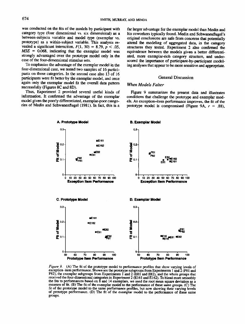
Figure 9 summarizes the present data and illustratesconditions that challenge the prototype and exemplar mod-els. As exception-item performance improves, the fit of theprototype model is compromised (Figure 9A, r - .88),

A. Prototype Model

0.3-,

i 0.2-

"5£0.1

•EB1

•E161

•E162

E82

P81

0 10 20 30 40 50 60 70 80 90 100Exception Item Performance

B. Exemplar Model

| 0 . ,

s

£0.1-

0-

P82

1 1 1

E

E81

i

•E161

1 1 1 1

0 10 20 30 40 50 60 70 80 90 100Exception Item Performance

C. Prototype Model

0.3 n

> 0.2-

•E161

•E162

•E81•EB2

50 60 70 80 90 100Prototype Hem Performance

D. Exemplar Model

0.3 n

0.2-

"5£0.1 •E16

•E1

50 60 70 80 90 100Prototype Item Performance

Figure 9. (A) The fit of the prototype model to performance profiles that show varying levels ofexception-item performance. Shown are the prototype subgroups from Experiments 1 and 2 (P81 andP82), the exemplar subgroups from Experiments 1 and 2 (E81 and E82), and the whole groups thatreceived the four-dimensional categories in Experiment 2 (E161 and E162). To blend more smoothlythe fits to performances based on 8 and 14 exemplars, we used the root mean square deviation as ameasure of fit. (B) The fit of the exemplar model to the performance of these same groups. (C) Thefit of the prototype model to the same performance profiles, but now showing their varying levelsof prototype performance. (D) The fit of the exemplar model to the performance of these samegroups.

LINEAR SEPARABILITY 675

whereas the exemplar model fits better (Figure 9B, r =— .94). Conversely, as prototype performance improves, theprototype model fits better {Figure 9C, r = -.88), whereasthe exemplar model falters (Figure 9D, r = .75).

Thus the exemplar model performs worse when fittingheterogenized performance, with larger prototype effectsand lower exception-item performance. This is why it fitspooriy the performance profiles of the prototype participants(Figures 5 and 7) and fits well the performances shown inFigure 8. The model has this character because it letsexemplars retrieve themselves, and this self-retrieval cansupport correct categorizations. The prototypes and theexception items, experienced repeatedly in training, can bothrely on these self-retrieval episodes and this brings theirlevels of performance closer together. Moreover, eventhough the prototype is surrounded by similar exemplars, theone-dimensional mismatches can reduce multiplicative simi-larity to the point where "close" neighbors contributenegligibly to processing and hardly boost prototype perfor-mance. This is especially true for high sensitivity (low-similarity parameters) in the exemplar model and for thepresent case in which the prototypes were experiencedin training.

In contrast, the prototype model performs better whenprototype and exception-item performance diverge most.Calling an exceptional category member a nonmember, andmaking NLS categories into LS ones by reassigning excep-tions, axe the specialties of the prototype model. The modelhas this character because there is no exemplar self-retrievalthat can increase exception performance. Also, the prototypehas perfect self-similarity, producing strong prototype effects.

Interpreting the Performance of PrototypeParticipants

Figure 10A shows the prototype and exception-itemperformance for each of the 16 prototype participants inExperiments 1 and 2. These participants have failed to learnthe six-dimensional NLS categories, in the sense favored byMedin and his coworkers, of being able to accept allcategory members and reject all nonmembers (Medin &Schwanenflugel, 1981; Wattenmaker et al., 1986). Theirperformance shows the problematic nature of the exceptionsand the reallocation of these items into the opposingcategories. Through this reallocation, participants haveturned the NLS categories into good LS ones. To do so, theyhave ignored errors, feedback, the experimenter's categorydefinitions, and even the possibility of exemplar memoriza-tion. For them, there is a linear separability constraint atwork. This is why the prototype model accounts easily,naturally, and best for these performances. Emphasizing thispoint, Figure 10B samples the entire constellation of perfor-mance profiles that are producible by the prototype model.This figure was created by moving systematically throughall 1,115,730 parameter settings of a fine grained scan of theprototype model and capturing the average prototype perfor-mance and exception-item performance predicted by arandom one in three hundred of these simulated observers.Prototype participants lie comfortably in the region ofperformance space covered by the prototype model.

A. Prototype Subject*

0 10 20304050S0708090 100Prototype Item Performance

B. Prototype-Based Performance

sIIQ.

O

1

100

90

80-

70-

60

50

40

30-

20^

10

010 20 30 40 50 60 70 80 90 100

Prototype Item Performance

Exemplar-Based Performance

0 10 20 30 40 50 60 70 80 90 100

Prototype Item Performance

Figure 10. (A) Average prototype-item performance and excep-tion-item performance for the 16 prototype participants fromExperiments 1 and 2. (B) Average prototype-item performance andexception-item performance for about 3,700 parameter settings ofthe prototype model, randomly chosen during a detailed scan of itsparameter space. (C) Average prototype-item performance andexception-item performance for about 5,400 parameter settings ofthe exemplar model, randomly chosen during a detailed scan of itsparameter space.

676 SMITH, MURRAY, AND MINDA

In contrast, the performance patterns of the prototypeparticipants fit poorly with some ideas about exemplar-basedcategorization strategies. One wonders why the participantsdid not just memorize the exemplars, especially the excep-tions, and let these traces guide the correct categorization.One wonders why they did not code the problematic stimulimore relationally, noting the appropriate label for thatparticular constellation of features. Even after nearly 400trials (in Experiment 2), they have not done so.

Emphasizing this point, Figure IOC samples the entireconstellation of performance profiles that are producible bythe exemplar model. This figure was created by movingsystematically through all 19,487,171 parameter settings ofa fine grained scan of the exemplar model and capturing theaverage prototype performance and exception-item perfor-mance predicted by a random 1 in 5,000 of these simulatedobservers. For this purpose, to ensure that no relevantperformance profiles were excluded, the exemplar modelwas granted a seventh free parameter that evaluated differentrates of guessing. As shown by the figure, many prototypeparticipants lie outside this region of performance space(and the earlier simulations confirmed that chance events donot explain this). The exemplar model can predictexception-item performance as low as that shown by someof these participants. However, then it seriously underpre-dicts their prototype performance. The exemplar model canpredict prototype performance as high as that shown bythese participants. However, then it seriously overpredictstheir exception-item performance. The prototype partici-pants were fit poorly because they required the model toaccomplish two goals that are incompatible given its behav-ior. The simplest interpretation is that prototype participantswere using a prototype strategy that subjected them to alinear separability constraint.

Illustrating the existence of these participants, and thelinear separability constraint they operate under, was theprimary goal of the present research, for it represents auseful counterweight to existing research. The presentcategory structures have not induced strong prototype strate-gies and an LS constraint in all participants, but clearly thatapproach gains (and reaches parity) in the transition from thecategory structures of previous research (e.g., the four-dimensional categories of Experiment 2) to the six-dimensional categories of Experiments 1 and 2. This parityis not just a technical or formal equivalence born, forexample, from the ceiling performance that both modelswould predict at high structural ratios. Rather, the exemplarmodel is failing in a predictable way to capture theperformance profiles of many participants. These prototypeparticipants are important because they have been anendangered species lately in the categorization literature.

Different Category Structures That Foster DifferentTask Psychologies

Why is the prototype strategy more prominent in our datathan in previous research? Structural differences betweenstimulus sets must underlie these differences. The four-dimensional stimulus sets used here and in many previousstudies have fewer stimuli that are repeated sooner and more

often during the experiment. They contain less differentiatedcategories and less deviant exception items. The structuralratio of 1.32 means that similarity is fairly homogeneouslydistributed between and within categories. The six-dimen-sional stimulus set used here had the opposite character inevery respect.

These structural differences could produce different taskpsychologies or strategies. With fewer stimuli, exemplarmemorization will be easier. With more repetitions, thatstrategy will be more obvious, even as the specific traces arereinforced. With less differentiated categories, the urge toform LS exemplar clusters will be weakened. For example,no big dissimilarity jumps between successive stimuli willsignal that there are two well-organized groups of exem-plars. With less deviant exceptions, there will be less"remorse" about including them in the correct category. Thepresent six-dimensional stimulus set, by contrast, featuredmore stimuli to bookkeep, fewer repetitions to aid thisprocess, more pull to the prototypes, and more proble-matic exceptions.

Further research will be needed to pinpoint which of thesestructural differences produced the strategy differences ob-served across conditions. For example, one might be able tomanipulate independently the dimensionality of the stimulusset, the number of exemplars in categories, and the similaritystructure of the categories, to see which factor is implicatedmost strongly. The balance between prototype and exemplarmodels, in all four conditions of Experiment 1, couldsuggest that the larger exemplar pools there either encour-aged prototype strategies or discouraged exemplar strate-gies. However, possibly against this idea, McKinley andNosofsky (1995) found that participants, after thousands oftraining trials, were able to defend nonlinear decisionboundaries even given scores of unique stimuli.

Another possibility is that assimilation to prototypesgrows stronger at better levels of category structure so matitem-specific information is lost that could support thecorrect categorization of exceptions. However, against thisidea is the fact that the modest structural ratio manipulationin Experiment 1 did not produce this effect. More generally,we believe that error signals are a powerful signal toparticipants that they need to adopt new strategies incategorization.

This discussion leads us to contrast two different configu-rations of categorization research. One configuration fea-tures small exemplar pools, poorly differentiated categories,learning difficulties, weak prototype effects, relatively strongexception-item performance, homogenized performanceoverall, and the comfortable fit of the exemplar model,plausibly indicating exemplar-based strategies. Such strate-gies would have a sound information-processing basis. Asprototype strategies are undermined by impoverished simi-larity relationships, frequent error signals could promptstrategy changes, while frequent exemplar repetition re-minds the participant about exemplar-memorization strate-gies and even builds the strongly individuated traces thatserve them. Thus, this configuration of category structure,information-processing strategy, performance profile,and best fitting model might be a mutually reinforcing,closed system.

LINEAR SEPARABILITY 677

Another configuration of categorization research involveslarger exemplar pools, well-differentiated categories, easierlearning, strong prototype effects, poor exception-itemperformance, heterogenized performance overall, and thecomfortable fit of the prototype model, plausibly indicatingprototype-based strategies. Again, these strategies wouldhave a sound information-processing basis. As prototypestrategies succeed, rare error signals would discouragestrategy changes, while larger exemplar pools camouflageand undermine the exemplar-based alternatives. This configu-ration of structure, processing, performance, and modelcould also be a mutually reinforcing, closed system. We donot prejudge which configuration is more generally appli-cable and true—either in the laboratory or in the naturalecology. Our point is only that both configurations havepotential importance, both in the laboratory and in thenatural ecology.

However, one must explore fully the broad range ofcategory structures to know if this is true. It continues to befashionable to inflict extraordinarily difficult category struc-tures on participants. These structures do allow beautifulstimulus control and elegant modeling, but there may be acost. Just as objects look red in red light, so categorylearning may look exemplar based for as long as only anexemplar-sparse, poorly differentiated light is shed on it.

Epochs of Learning and Models of Categorization

Another perspective on our results comes from supposingthat we observed participants during some early phase oflearning (lasting through 392 trials), when the prototypeparticipants were only about 25% correct on the exceptions.Even though we gave participants more trials than in thedirectly comparable studies, related experiments have some-times given thousands of trials. If learning had gone onmuch Longer, would not participants have mastered theexceptions finally, and would not the exemplar model havefit better then?

This possibility raises important issues. If one madeparticipants persist until they learned the exceptions, thehomogeneous performance landscape that resulted wouldfavor the exemplar model. This advantage is not justcircular—even though the criterion for ceasing trainingwould be a comfortable configuration for the exemplarmodel (i.e., one in the top-right quadrant of the graphs inFigure 10). Participants' success would show that they caneventually transcend the difficulty of the exception items,possibly by applying special learning algorithms (e.g.,exemplar memorization, etc.). However, equally interestingis the fact that here many participants made little headwaywith the exceptions even after 28 presentations of them.These participants are in a serious rut with prototypy andlinear separability, and this is an extended stage of learning,even if they eventually transcend it.

The implication of this is that different training regimensused in category research make different commitments. Forexample, Nosofsky (1986), hoping to model a fully matureperformance, tested participants on 1,200-trial blocks untilthey performed better than chance on all stimuli in the last600 trials of a block. (In other studies Nosofsky modeled

performance earlier in learning; e.g., see Nosofsky, 1989.)This extensive training eliminates poor performance on any"exception" items, homogenizes performance in the mannerrelevant here, and favors the exemplar model appropriatelybecause of participants' eventual success. However, thistraining regimen chooses not to ask if participants wentthrough important prototype-based epochs earlier in training.

If one chooses to ask, one may find different kinds ofprocesses, and different kinds of best fitting models, duringdifferent epochs of training and learning. Studying eventualtranscendance over exceptions is not the only importantissue in categorization research. Default assumptions, firstprinciples, general preferences, and mode chosen givencooperative circumstances—these are all equally plausibleareas of investigation. Curiously, all of these could beprototype based, and all of these could enforce a linearseparability constraint, but it could still be true that intensetraining would transcend the limits of these strategies andconstraints and bring favor on the exemplar model. Thesedefault or preferred strategies have received scant researchattention—at least until very recently.

For example, Ahn and Medin (1992) and Nosofsky et al.(1994) both suggested that participants learn categories byfirst making a straight, linear cut through the stimulus world,using a single-dimensional rule (see also results from sortingparadigms in Medin, Wattenmaker, & Hampson, 1987;Regehr & Brooks, 1995). Then, to the extent that the ruleproduces errors, participants invoke special learning algo-rithms to master the exceptions. These algorithms caninvolve exemplar memorization or the relational coding offeatural complexes that need special classificatory process-ing. In an elegant demonstration of different learningepochs, Nosofsky et al. considered category structures thatallowed generalization by either independent informativecues or by relational cues (correlated attributes). Theyshowed that generalizations made early in learning followedindividual diagnostic cues, whereas later generalizationsfollowed relational coding.

These descriptions of categorization deemphasize thestatic context model and the idea that humans are pure,relational-coding creatures with exemplar-blotter memories.They emphasize that different epochs of learning involvedifferent strategies and varieties of stimulus coding. Theyfavor the idea that the default options and early epochsinvolve a strong linear separability assumption. They linkrelational coding to the special learning algorithms thatcome later in learning, and only if necessary. They suggestthat the exemplar model will find progressively more favorlater in learning because its kind of processing is allied to theeventual-transcendance strategies that conquer exceptions.

We endorse each of these conclusions. In turn, thesemodels endorse our view about the problems and theprocessing consequences of poor category differentiation.Poorer category differentiation will guarantee less adequaterules, demand more focus on their exceptions, require morerelational coding, and may well favor the exemplar modelmore. The only suggestion we would add is that early rulesneed not just be unidimensional. We believe that participantscan also rapidly appreciate multidimensional hypotheses or

678 SMYTH, MURRAY, AND MINDA

rules and then set to work on the exceptions to theseprototypes. This phenomenon may be best seen by providingbetter differentiated category structures—we believe thatprototype strategies may especially accrete around well-differentiated prototype cores.

These converging perspectives on categorization arewelcome. At times the combination of poorly differentiatedcategory structures and demonstrations of eventual transcen-dance may have confined theories of categorization toomuch. Researchers have often placed participants in adifficult, exemplar-sparse corner of the domain of categoriza-tion, where exemplar models may be favored, and whereprototype strategies may not even work. But then, research-ers have patiently kept training while participants masterthese difficult categories. They do, and exemplar models fitwell then because they should. This result is an importantexistence proof about participants* ultimate capacities incategorization. However, it may not be a subsistence proofabout what humans do during categorization's "business asusual" in the natural ecology. Subsistence categorization,

not just tour de force categorization, deserves researchers'careful study too.

The Real LS Advantage

This distinction leads us to move beyond our particularresults and to close by reconsidering some prevalent ideas inthe literature today—that there is a kind of equivalencebetween LS and NLS categories, that humans do not benefitfrom linear separability in learning categories, and that thereis no linear separability advantage or constraint (Ashby &Gott, 1988, p. 51; Kemler Nelson, 1984, p. 747; Lingle et al.,1984, pp. 93-94; McKinley & Nosofsky, 1995; Medin &Schwanenflugel, 1981; Murphy & Medin, 1985, p. 295;Wattenmakeretal., 1986, pp. 160-162).

These ideas have many roots. Demonstrating eventualtranscendence highlights equivalence because participantseventually do learn NLS categories. It is easy to forget theextensive training that attends their learning. The originalLS-NLS comparisons highlighted equivalence because NLS

B.

1 1.25 1.5 1.75 2 2.25 2.5 2.75

Structural Ratio (Additive)

• t - .

0.9-

0.8-

• 0.7-

;o.e-

.0.51 1.25 1.5 1.75 2 2.25 2.5 2.75

Structural Ratio (Additive)

C. D.

"S.13-E| iH

7 »

1 ••% 3

1 1.25 1.5 1.75 2 2.25 2.5 2.75

Structural Ratio (Additive)

0.9-

0.8-

! 0.6-

0.0.5155 1.5 1.75 2 2.26 2.5 2.75

Structural Ratio (Additive)

Figure II. (A) Seven hundred hypothetical category structures illustrating the range of categorydifferentiation offered by linearly separable categories. (B) The overall performance of a genericconfiguration of the exemplar context model (dimensional weights - .45) on those 700 LS stimulussets. (C) Seven hundred hypothetical category structures illustrating the range of categorydifferentiation offered by nonlinearly separable categories. (D) The overall performance of the sameconfiguration of the exemplar model on those 700 NLS stimulus sets.

LINEAR SEPARABILITY 679

categories did not produce poorer learning there. It is easy toforget the skillful balancing of similarity relations that madeequivalent performance the natural outcome of these experi-ments, and it is easy to drift beyond the careful specificity ofthe original claims in this area. Following on the research,equivalence was suggested because exemplar memorizationcould balance prototypy and support the learning of NLScategories, because relational-coding schemes could letparticipants encode strongly individuated exemplars andcategorize them correctly, because the correlations betweenattributes could support the mastery of some NLS catego-ries, and because conceptual and theoretical knowledgecould also support the learning of NLS categories that arepoorly structured perceptually.

In contrast, Figure 11 illustrates a basic nonequivalencebetween LS and NLS category structures. Figure 11A shows700 hypothetical linearly separable category structures bystructural ratio, and Figure 11B shows how well a genericexemplar-based categorizer (with parameter settings of .45on each dimension) would perform overall on each of them.Not surprisingly, there is a strong relationship betweenoverall performance and category differentiation. The samewould be true of a prototype-based categorizer. The morel isthat mushroom foragers should fervently hope that edibleand poisonous mushroom categories will be well differenti-ated. Predator avoiders should fervently hope that eagle andvulture categories will be well differentiated. If they are, thespecies will eat better—longer.

Figure 11C shows the similarity relationships for 700hypothetical NLS category structures constructed as here,with one exception item in each category. Figure 11D showsthe performance of the exemplar-based categorizer again.Figure 11 makes a point that is sometimes lost in studies ofcategorization and linear separability. On average, LS catego-ries will be better differentiated. On average, LS categorieswill be more easily learned and performed at a higher level.The fact of NLS weakens the similarity relationships withincategories and reduces the structural ratio for a pair ofcategories. The fact of NLS damages the performance of theexemplar-based (and prototype-based) categorizer. The 75%levels of performance shown in Figure 11D could spell realdisaster for a real species that mistook, one fourth of thetime, poisonous mushrooms for edible ones and eagles forvultures. The species would eat worse—and worse, be eaten.

Furthermore, in a case like this the eventual capacity totranscend the poor perceptual structure and master the wholecategory is not the vital issue. The equality of performanceon two carefully selected category structures that are per-fectly balanced for similarity is also not the vital issue.Rather, the vital issue is how long do categories take tolearn, and how difficult are they to learn, with thesequestions given urgency by the seriousness of mistakes inthe natural world.

On this vital issue both exemplar-based and prototype-based models agree. Over the whole range of categorystructures available, as assessed by the two most prominentmodels of cognitive processing in categorization tasks, therehas always been, and there will always be, a profound linearseparability advantage.

References

Ann, W., & Medin, D. L. (1992). A two-stage model of categoryconstruction. Cognitive Science, 16, 81-121.

Ashby, F. G., & Gott, R. E. (1988). Decision rules in the perceptionand categorization of multidimensional stimuli. Journal ofExperimental Psychology: Learning, Memory, and Cognition,14t 33_53,

Hartley, J,, & Homa, D. (1981). Abstraction of stylistic concepts.Journal of Experimental Psychology: Human Learning andMemory, 1, 33-46.

Homa, D., Rhoads, D., & Chambliss, D. (1979). Evolution ofconceptual structure. Journal of Experimental Psychology: Hu-man Learning and Memory, 5, 11-23.

Homa, D., Sterling, S., & Trepel, L. (1981), Limitations ofexemplar-based generalization and the abstraction of categoricalinformation. Journal of Experimental Psychology: Human Learn-ing and Memory, 7,418-439.

Kemler Nelson, D. G. (1984). The effect of intention on whatconcepts are acquired. Journal of Verbal Learning and VerbalBehavior, 23, 734-759.

Ungle, J. H., Altom, M. W., & Medin, D. L. (1984). Of cabbagesand kings: Assessing the extendibility of natural object conceptmodels to social things. In R. S. Wyer & T. K. Srull (Eds.),Handbook of social cognition (pp. 71-117). Hillsdale, NJ:Erlbaum.

Locke, J. (1959). An essay concerning human understanding (A. C.Fraser, Ed.). New York: Dover. (Original work published 1690)

Malt, B. C , & Smith, E. E. (1984). Correlated properties in naturalcategories. Journal of Verbal Learning and Verbal Behavior, 23,250-269.

McKinley, S. C , & Nosofsky, R. M. (1995). Investigations ofexemplar and decision bound models in large, ill-defined cat-egory structures. Journal of Experimental Psychology: HumanPerception and Performance, 21,128-148.

Medin, D. L., Altom, M. W., Edelson, S. M., & Freko, D. (1982).Correlated symptoms and simulated medical classification. Jour-nal of Experimental Psychology: Learning, Memory, and Cogni-tion, 8, 37-50.

Medin, D. L., Dewey, G. I., & Murphy, T. D. (1983). Relationshipsbetween item and category learning: Evidence that categoriza-tion is not automatic. Journal of Experimental Psychology:Learning, Memory, and Cognition, 9, 607-625.

Medin, D. L., & Schaffer, M. M. (1978). Context theory ofclassification learning. Psychological Review, 85, 207-238.

Medin, D. L., & Schwanenflugel, P. J. (1981). Linear separability inclassification learning. Journal of Experimental Psychology:Human Learning and Memory, 75, 355-368.

Medin, D. L., & Smith, E. E. (1981). Strategies and classificationlearning. Journal of Experimental Psychology: Human Learningand Memory, 7, 241-253.

Medin, D. L., Wattenmaker, W. D., & Hampson, S. E. (1987).Family resemblance, conceptual cohesiveness, and categoryconstruction. Cognitive Psychology, 19, 242-279.

Mervis, C. B., & Rosch, E. (1981). Categorization of naturalobjects. Annual Review of Psychology, 32, 89-115.

Murphy, G. L., & Medin, D. L. (1985). Role of theories inconceptual coherence. Psychological Review, 92, 289-316.

Nosofsky, R. M. (1984). Choice, similarity, and the context theoryof classification. Journal of Experimental Psychology: Learning,Memory, and Cognition, 10, 104—114.

Nosofsky, R. M. (1986). Attention, similarity, and the identification-categorization relationship. Journal of Experimental Psychol-ogy: General, 115, 39-57.

Nosofsky, R. M. (1987). Attention and learning processes in theidentification and categorization of integral stimuli. Journal of

680 SMITH, MURRAY, AND M1NDA

Experimental Psychology: Learning, Memory, and Cognition,13, 87-108.

Nosofsky, R. M. (1989). Further tests of an exemplar-similarityapproach to relating identification and categorization. Percep-tion & Psychophysics, 45, 279-290.

Nosofsky, R. M. (1992). Exemplars, prototypes, and similarityrules. In A. R Healy, S. M. Kosslyn, & R. M. Shiffrin (Eds.),From learning theory to connectionist theory: Essays in honor ofWilliam K. Estes (pp. 149-167). HUlsdale, NJ: Eribaum.

Nosofsky, R. M., Palmeri, T. J., & McKinley, S. K. (1994).Rule-plus-exception model of classification learning. Psychologi-cal Review, 707,53-79.

Posner, M. I., & Keele, S. W. (1968). On the genesis of abstractideas. Journal of Experimental Psychology, 77, 353-363.

Posner, M. I., & Keele, S. W. (1970). Retention of abstract ideas.Journal of Experimental Psychology, 83, 304-308.

Regehr, G., & Brooks, L. (1995). Category organization in freeclassification: The organizing effect of an array of stimuli.Journal of Experimental Psychology: Learning, Memory, andCognition, 21, 347-363.

Rosch, E. (1973). On the internal structure of perceptual andsemantic categories. In T. E. Moore (Ed.), Cognitive develop-ment and the acquisition of language (pp. 111-144). New York:Academic Press.

Rosch, E. (1975). Cognitive reference points. Cognitive Psychol-ogy, 7, 192-238.

Rosch, E., & Mervis, C. B. (1975). Family resemblances: Studiesin the internal structure of categories. Cognitive Psychology, 7,573-605.

Sebestyen, G. S. (1962). Decision-making processes in patternrecognition. New York: Macmillan.

Shepard, R. N., Hovland, C. I., & Jenkins, H. M. (1961). Learningand memorization of classifications. Psychological Mono-graphs, 75 (13, Whole No. 517).

Smith, E. &, Shoben, E. J., & Rips, L. J. (1974). Structure andprocess in semantic memory: A featural model for semanticdecision. Psychological Review, 81, 214-241.

Smith, J. D. (1989). Analytic and holistic processes in categoriza-tion. In B. E. Shepp & S. Ballesteros (Eds.), Object perception:Structure and processes (pp. 297-323). Hillsdale, NJ: Eribaum.

Smith, J. D., & Shapiro, J. H. (1989). The occurrence of holisticcategorization. Journal of Memory and Language, 28, 386-399.

Smith, J. D., Tracy, J., & Murray, M. J. (1993). Depression andcategory learning. Journal of Experimental Psychology: Gen-eral, 122, 331-346.

Wattenmaker, W. D., Dewey, G. I., Murphy, T. D., & Medin, D. L.(1986). Linear separability and concept learning: Context,relational properties, and concept naturalness. Cognitive Psychol-ogy, 18,158-194.

Whittlesea, B. W. A. (1987). Preservation of specific experiences inthe representation of general knowledge. Journal of Experimen-tal Psychology: Learning, Memory, and Cognition, 13, 3-17.

Whittlesea, B. W. A., Brooks, L., & Westcott, C. (1994). After thelearning is over: Factors controlling the selective application ofgeneral and particular knowledge. Journal of ExperimentalPsychology: Learning, Memoryi and Cognition, 20, 259-274.

Appendix

Category Structures Used in Experiment 1

Categories linearly separable

Category A

Structure

10100010001010000101 10000 1 0 1 0 00 0 1 0 0 10 0 0 0 1 1

0 0 0 0 0 01000000 1 0 0 0 010000101 10000 0 1 0 1 00 0 0 1 0 1

Stimuli

Category B

Structure

Difficult

LITUPOLIRUNOLIRUPYGETUPOGERAPOGITUPYGIRUNY

001 1 1 10 1 1 0 1 101 1101101011101 1 101 101011 1 1 100

Easy

BUNOLIKUNOLIBYNOLIKUNOLABYPOLIBUPORIBUNELA

1111111101111111010 1 0 1 1 10 1 1 1 1 0101011101 1 10

Stimuli

GITANYGETUNYGETAPYLITUNYLITANOLERAPYLETAPO

KYPERAKYNERAKYPELABYNERABYPERIKUPORAKUPERI

Categories not linearly separable

Category A

Structure

0 1 0 0 0 00 0 1 0 0 0000001101000100010001001110111

000000100000010000001000000010000001111101

Stimuli

Category B

Structure

Difficult

GERUPOGITUPOGIRUPYLITUPOLIRUNOGITUPYLERANY

01 1 1 I 1101111111101011 1 101011011110010 0 0 0 1 0

Easy

BUNOLIKUNOLIBYNOLIBUPOLIBUNORIBUNOLAKYPELA

1 1 1 1 I 101 11 111011111101111 1 101 1111110000100

Stimuli

GETANYLITANYLETAPYGETANOLITAPYLETUPYGIRUNO

KYPERABYPERAKUPERAKYNERAKYPORAKYPERIBUNELI

Received September 14,1995Revision received August 7, 1996

Accepted August 15, 1996

View publication statsView publication stats