Storage

04/21/23 2

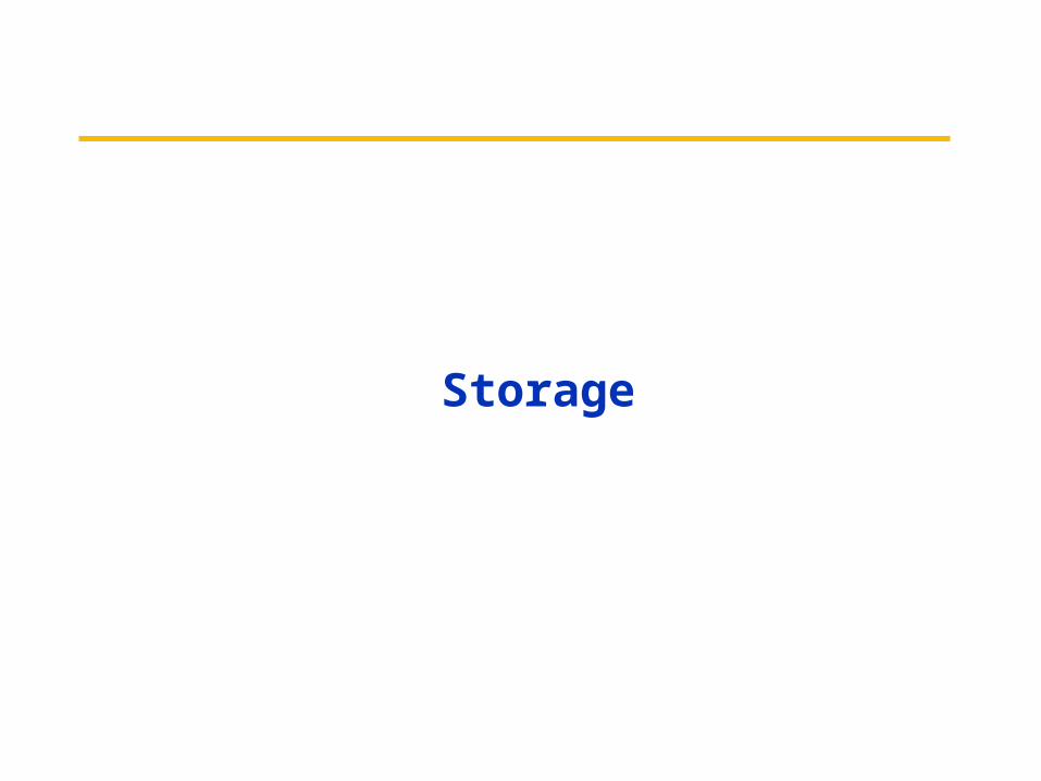
Case for Storage

• Shift in focus from computation to communication and storage of information

– E.g., Cray Research/Thinking Machines vs. Google/Yahoo– “The Computing Revolution” (1960s to 1980s)

“The Information Age” (1990 to today)

• Storage emphasizes reliability and scalability as well as cost-performance

• What is “Software king” that determines which HW acually features used?

– Operating System for storage– Compiler for processor

• Also has own performance theory—queuing theory—balances throughput vs. response time

04/21/23 3

Outline

• Magnetic Disks

• RAID

• Advanced Dependability/Reliability/Availability

• I/O Benchmarks, and Performance

• Conclusion

04/21/23 4

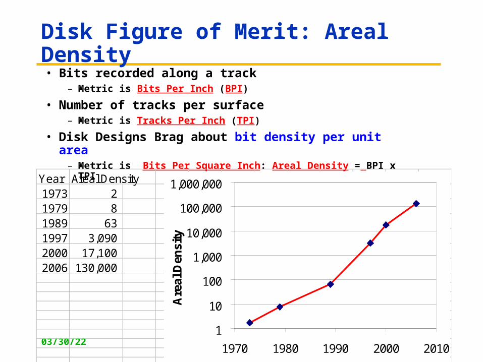
Disk Figure of Merit: Areal Density• Bits recorded along a track

– Metric is Bits Per Inch (BPI)

• Number of tracks per surface– Metric is Tracks Per Inch (TPI)

• Disk Designs Brag about bit density per unit area– Metric is Bits Per Square Inch: Areal Density = BPI x TPI

Year Areal Density1973 2 1979 8 1989 63 1997 3,090 2000 17,100 2006 130,000

1

10

100

1,000

10,000

100,000

1,000,000

1970 1980 1990 2000 2010

Year

Are

al D

ensi

ty

04/21/23 5

Historical Perspective

• 1956 IBM Ramac — early 1970s Winchester– Developed for mainframe computers, proprietary interfaces– Steady shrink in form factor: 27 in. to 14 in.

• Form factor and capacity drives market more than performance• 1970s developments

– 5.25 inch floppy disk formfactor (microcode into mainframe)– Emergence of industry standard disk interfaces

• Early 1980s: PCs and first generation workstations• Mid 1980s: Client/server computing

– Centralized storage on file server» accelerates disk downsizing: 8 inch to 5.25

– Mass market disk drives become a reality» industry standards: SCSI, IPI, IDE» 5.25 inch to 3.5 inch drives for PCs, End of proprietary interfaces

• 1900s: Laptops => 2.5 inch drives• 2000s: What new devices leading to new drives?

04/21/23 6

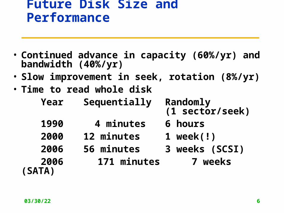
Future Disk Size and Performance

• Continued advance in capacity (60%/yr) and bandwidth (40%/yr)

• Slow improvement in seek, rotation (8%/yr)• Time to read whole disk

Year Sequentially Randomly (1 sector/seek)

1990 4 minutes 6 hours2000 12 minutes 1 week(!)2006 56 minutes 3 weeks (SCSI)2006 171 minutes 7 weeks (SATA)

04/21/23 7

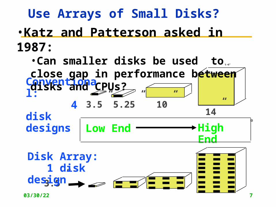
Use Arrays of Small Disks?

14”10”5.25”3.5”

3.5”

Disk Array: 1 disk design

Conventional: 4 disk designs

Low End High End

•Katz and Patterson asked in 1987: •Can smaller disks be used to close gap in performance between disks and CPUs?

04/21/23 8

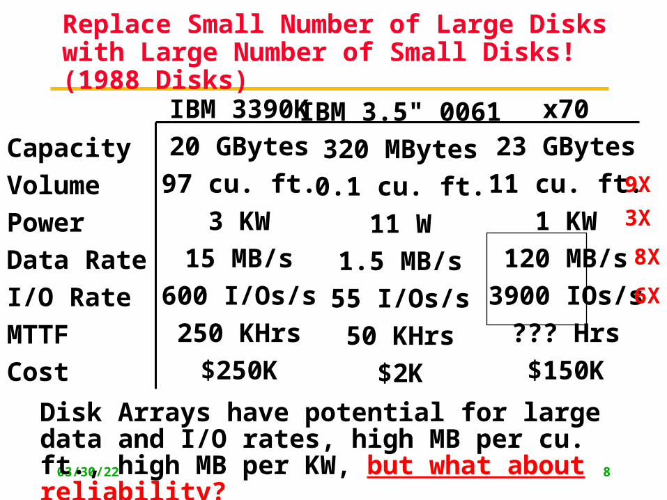
Replace Small Number of Large Disks with Large Number of Small Disks! (1988 Disks)

Capacity

Volume

Power

Data Rate

I/O Rate

MTTF

Cost

IBM 3390K

20 GBytes

97 cu. ft.

3 KW

15 MB/s

600 I/Os/s

250 KHrs

$250K

IBM 3.5" 0061

320 MBytes

0.1 cu. ft.

11 W

1.5 MB/s

55 I/Os/s

50 KHrs

$2K

x70

23 GBytes

11 cu. ft.

1 KW

120 MB/s

3900 IOs/s

??? Hrs

$150K

Disk Arrays have potential for large data and I/O rates, high MB per cu. ft., high MB per KW, but what about reliability?

9X

3X

8X

6X

04/21/23 9

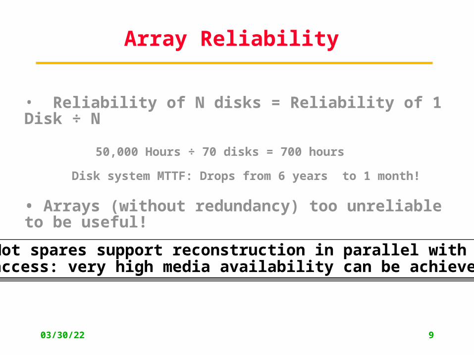
Array Reliability

• Reliability of N disks = Reliability of 1 Disk ÷ N

50,000 Hours ÷ 70 disks = 700 hours

Disk system MTTF: Drops from 6 years to 1 month!

• Arrays (without redundancy) too unreliable to be useful!

Hot spares support reconstruction in parallel with access: very high media availability can be achievedHot spares support reconstruction in parallel with access: very high media availability can be achieved

04/21/23 10

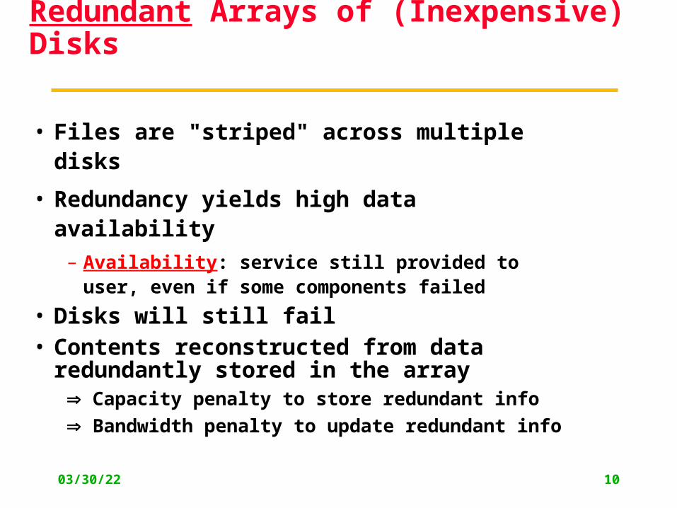
Redundant Arrays of (Inexpensive) Disks

• Files are "striped" across multiple disks

• Redundancy yields high data availability

– Availability: service still provided to user, even if some components failed

• Disks will still fail• Contents reconstructed from data redundantly

stored in the array Capacity penalty to store redundant info

Bandwidth penalty to update redundant info

04/21/23 11

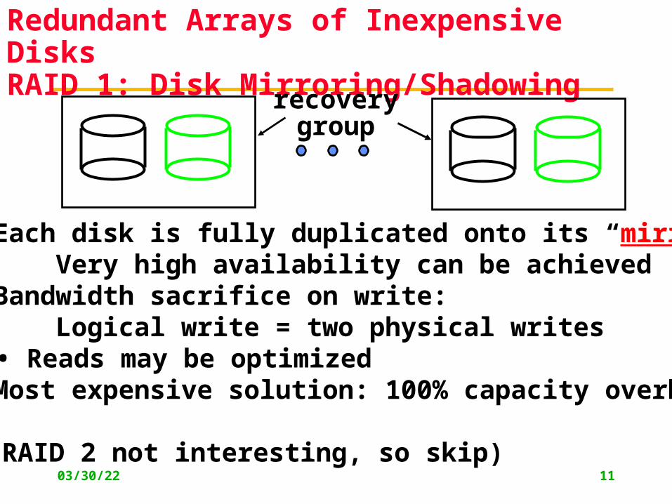
Redundant Arrays of Inexpensive DisksRAID 1: Disk Mirroring/Shadowing

• Each disk is fully duplicated onto its “mirror” Very high availability can be achieved• Bandwidth sacrifice on write: Logical write = two physical writes

• Reads may be optimized• Most expensive solution: 100% capacity overhead

• (RAID 2 not interesting, so skip)

recoverygroup

04/21/23 12

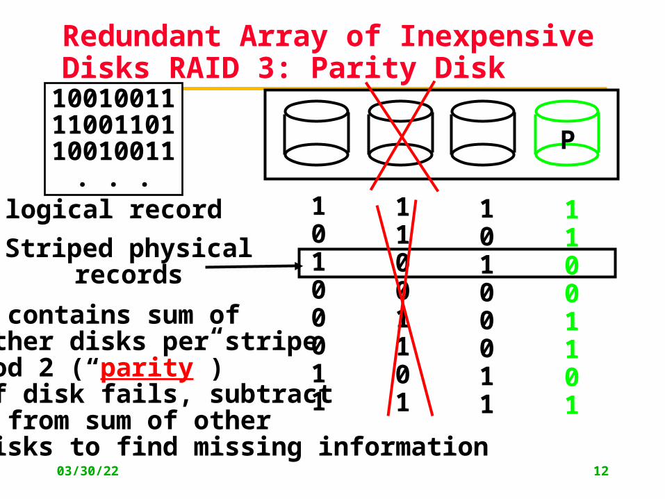
Redundant Array of Inexpensive Disks RAID 3: Parity Disk

P

100100111100110110010011

. . .logical record 1

0100011

11001101

10100011

11001101

P contains sum ofother disks per stripe mod 2 (“parity”)If disk fails, subtract P from sum of other disks to find missing information

Striped physicalrecords

04/21/23 13

RAID 3

• Sum computed across recovery group to protect against hard disk failures, stored in P disk

• Logically, a single high capacity, high transfer rate disk: good for large transfers

• Wider arrays reduce capacity costs, but decreases availability

• 33% capacity cost for parity if 3 data disks and 1 parity disk

04/21/23 14

Inspiration for RAID 4

• RAID 3 relies on parity disk to discover errors on Read

• But every sector has an error detection field• To catch errors on read, rely on error

detection field instead of the parity disk• Allows independent reads to different disks

simultaneously

04/21/23 15

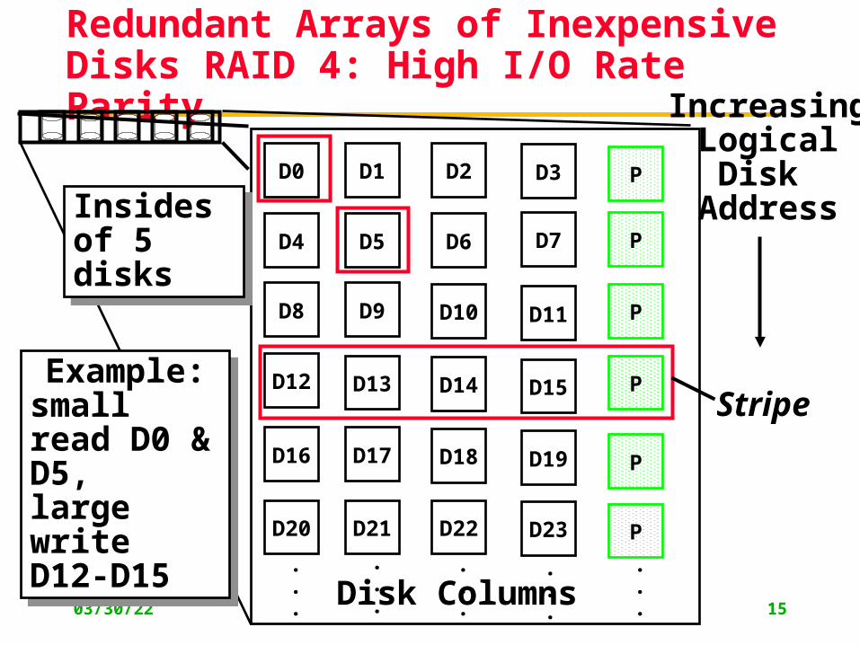
Redundant Arrays of Inexpensive Disks RAID 4: High I/O Rate Parity

D0 D1 D2 D3 P

D4 D5 D6 PD7

D8 D9 PD10 D11

D12 PD13 D14 D15

PD16 D17 D18 D19

D20 D21 D22 D23 P

.

.

.

.

.

.

.

.

.

.

.

.

.

.

.Disk Columns

IncreasingLogicalDisk

Address

Stripe

Insides of 5 disksInsides of 5 disks

Example:small read D0 & D5, large write D12-D15

Example:small read D0 & D5, large write D12-D15

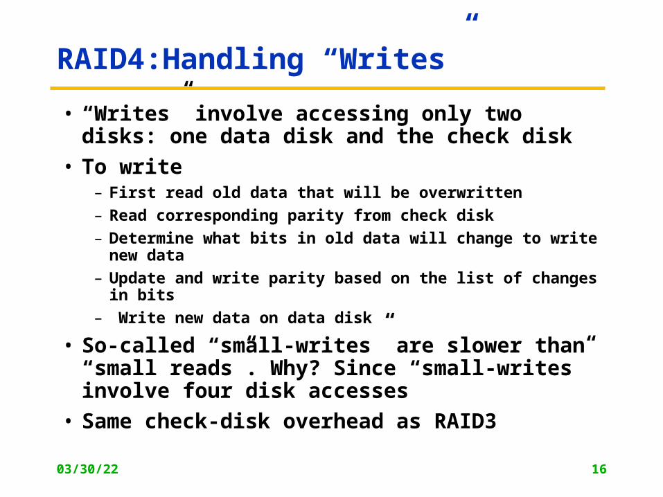
RAID4:Handling “Writes”

• “Writes” involve accessing only two disks: one data disk and the check disk

• To write– First read old data that will be overwritten

– Read corresponding parity from check disk

– Determine what bits in old data will change to write new data

– Update and write parity based on the list of changes in bits

– Write new data on data disk

• So-called “small-writes” are slower than “small reads”. Why? Since “small-writes” involve four disk accesses

• Same check-disk overhead as RAID3

04/21/23 16

04/21/23 17

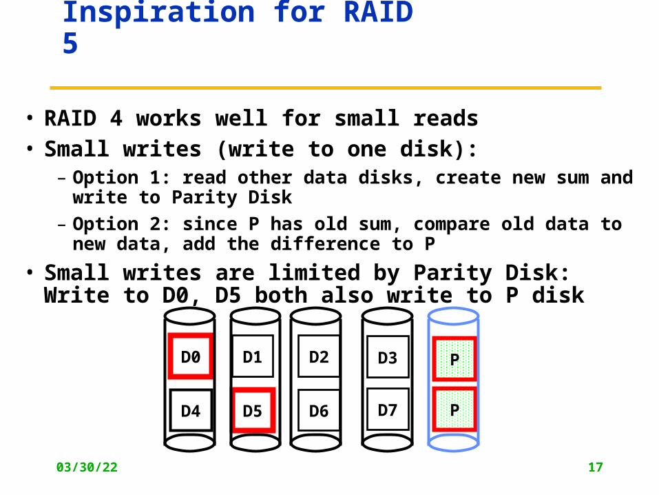
Inspiration for RAID 5

• RAID 4 works well for small reads• Small writes (write to one disk):

– Option 1: read other data disks, create new sum and write to Parity Disk

– Option 2: since P has old sum, compare old data to new data, add the difference to P

• Small writes are limited by Parity Disk: Write to D0, D5 both also write to P disk

D0 D1 D2 D3 P

D4 D5 D6 PD7

04/21/23 18

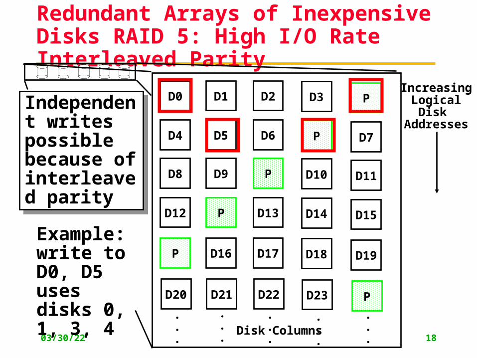
Redundant Arrays of Inexpensive Disks RAID 5: High I/O Rate Interleaved Parity

Independent writespossible because ofinterleaved parity

Independent writespossible because ofinterleaved parity

D0 D1 D2 D3 P

D4 D5 D6 P D7

D8 D9 P D10 D11

D12 P D13 D14 D15

P D16 D17 D18 D19

D20 D21 D22 D23 P

.

.

.

.

.

.

.

.

.

.

.

.

.

.

.Disk Columns

IncreasingLogical

Disk Addresses

Example: write to D0, D5 uses disks 0, 1, 3, 4

04/21/23 19

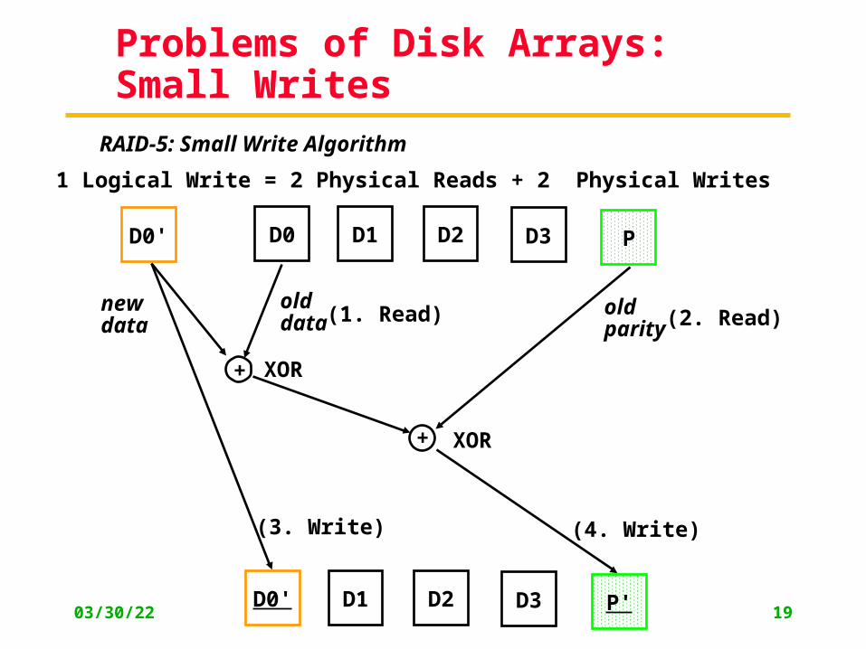
Problems of Disk Arrays: Small Writes

D0 D1 D2 D3 PD0'

+

+

D0' D1 D2 D3 P'

newdata

olddata

old parity

XOR

XOR

(1. Read) (2. Read)

(3. Write) (4. Write)

RAID-5: Small Write Algorithm

1 Logical Write = 2 Physical Reads + 2 Physical Writes

04/21/23 20

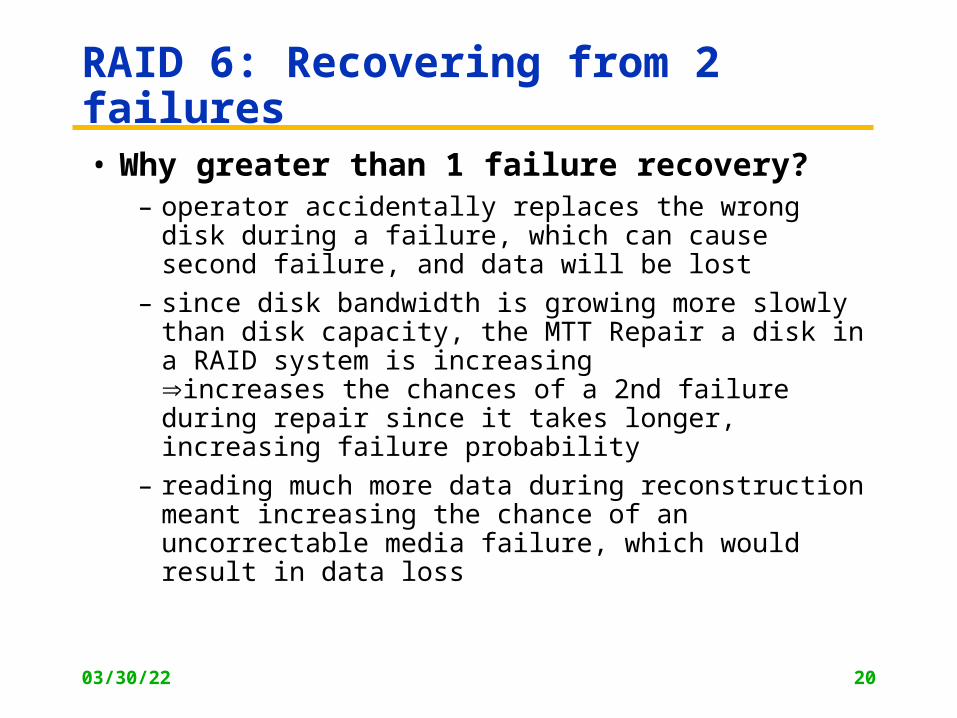
RAID 6: Recovering from 2 failures

• Why greater than 1 failure recovery?– operator accidentally replaces the wrong disk during a

failure, which can cause second failure, and data will be lost

– since disk bandwidth is growing more slowly than disk capacity, the MTT Repair a disk in a RAID system is increasing increases the chances of a 2nd failure during repair since it takes longer, increasing failure probability

– reading much more data during reconstruction meant increasing the chance of an uncorrectable media failure, which would result in data loss

04/21/23 21

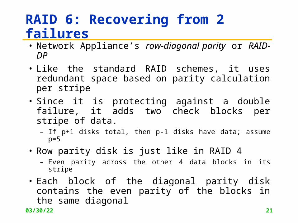
RAID 6: Recovering from 2 failures• Network Appliance’s row-diagonal parity or RAID-DP

• Like the standard RAID schemes, it uses redundant space based on parity calculation per stripe

• Since it is protecting against a double failure, it adds two check blocks per stripe of data.

– If p+1 disks total, then p-1 disks have data; assume p=5

• Row parity disk is just like in RAID 4 – Even parity across the other 4 data blocks in its stripe

• Each block of the diagonal parity disk contains the even parity of the blocks in the same diagonal

04/21/23 22

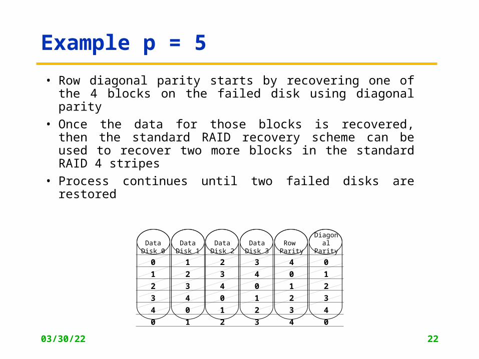
Example p = 5

• Row diagonal parity starts by recovering one of the 4 blocks on the failed disk using diagonal parity

• Once the data for those blocks is recovered, then the standard RAID recovery scheme can be used to recover two more blocks in the standard RAID 4 stripes

• Process continues until two failed disks are restored

Data Disk 0

Data Disk 1

Data Disk 2

Data Disk 3

Row Parity

Diagonal Parity

0 1 2 3 4 0

1 2 3 4 0 1

2 3 4 0 1 2

3 4 0 1 2 3

4 0 1 2 3 4

0 1 2 3 4 0

04/21/23 23

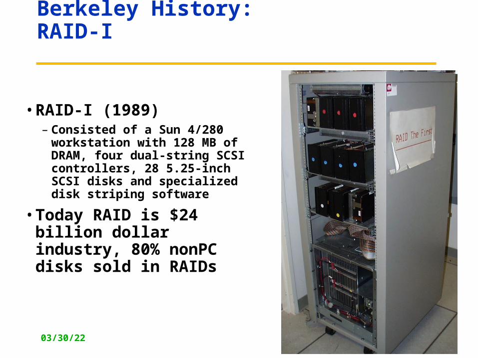
Berkeley History: RAID-I

• RAID-I (1989) – Consisted of a Sun 4/280

workstation with 128 MB of DRAM, four dual-string SCSI controllers, 28 5.25-inch SCSI disks and specialized disk striping software

• Today RAID is $24 billion dollar industry, 80% nonPC disks sold in RAIDs

04/21/23 24

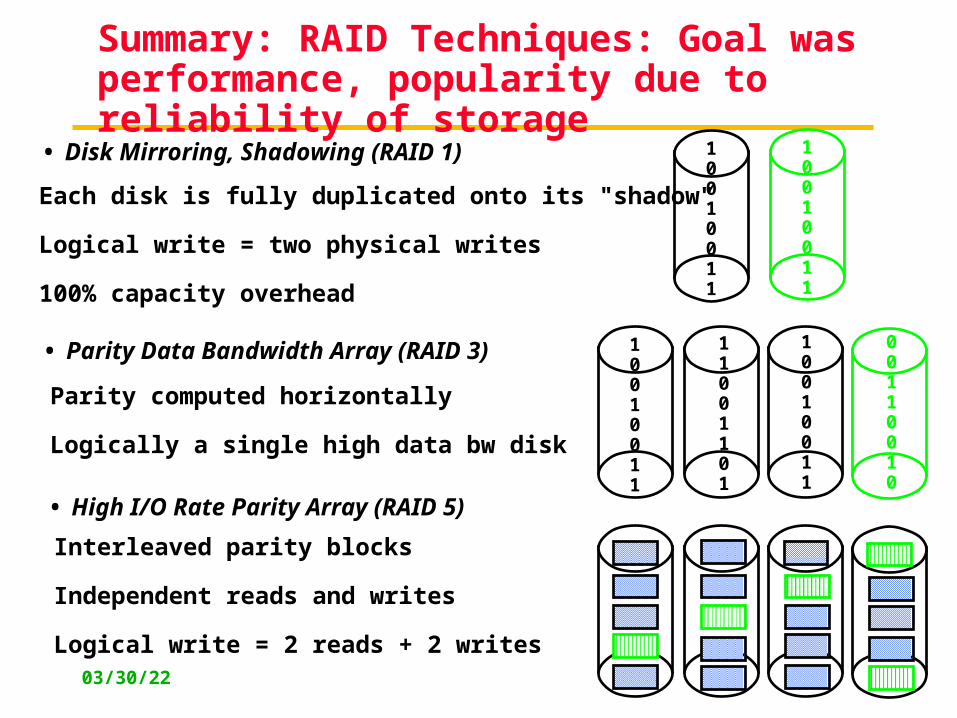
Summary: RAID Techniques: Goal was performance, popularity due to reliability of storage

• Disk Mirroring, Shadowing (RAID 1)

Each disk is fully duplicated onto its "shadow" Logical write = two physical writes

100% capacity overhead

• Parity Data Bandwidth Array (RAID 3)

Parity computed horizontally

Logically a single high data bw disk

• High I/O Rate Parity Array (RAID 5)

Interleaved parity blocks

Independent reads and writes

Logical write = 2 reads + 2 writes

10010011

11001101

10010011

00110010

10010011

10010011

04/21/23 25

Definitions

• Examples on why precise definitions so important for reliability

• Is a programming mistake a fault, error, or failure? – Are we talking about the time it was designed

or the time the program is run?

– If the running program doesn’t exercise the mistake, is it still a fault/error/failure?

• If an alpha particle hits a DRAM memory cell, is it a fault/error/failure if it doesn’t change the value?

– Is it a fault/error/failure if the memory doesn’t access the changed bit?

– Did a fault/error/failure still occur if the memory had error correction and delivered the corrected value to the CPU?

04/21/23 26

IFIP Standard terminology

• Computer system dependability: quality of delivered service such that reliance can be placed on service

• Service is observed actual behavior as perceived by other system(s) interacting with this system’s users

• Each module has ideal specified behavior, where service specification is agreed description of expected behavior

• A system failure occurs when the actual behavior deviates from the specified behavior

• failure occurred because an error, a defect in module

• The cause of an error is a fault

• When a fault occurs it creates a latent error, which becomes effective when it is activated

• When error actually affects the delivered service, a failure occurs (time from error to failure is error latency)

04/21/23 27

Fault v. (Latent) Error v. Failure

• An error is manifestation in the system of a fault, a failure is manifestation on the service of an error

• Is If an alpha particle hits a DRAM memory cell, is it a fault/error/failure if it doesn’t change the value?

– Is it a fault/error/failure if the memory doesn’t access the changed bit?

– Did a fault/error/failure still occur if the memory had error correction and delivered the corrected value to the CPU?

• An alpha particle hitting a DRAM can be a fault

• if it changes the memory, it creates an error

• error remains latent until effected memory word is read

• if the effected word error affects the delivered service, a failure occurs

04/21/23 28

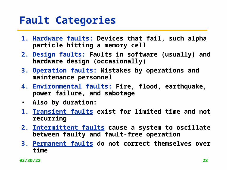
Fault Categories

1. Hardware faults: Devices that fail, such alpha particle hitting a memory cell

2. Design faults: Faults in software (usually) and hardware design (occasionally)

3. Operation faults: Mistakes by operations and maintenance personnel

4. Environmental faults: Fire, flood, earthquake, power failure, and sabotage

• Also by duration:

1. Transient faults exist for limited time and not recurring

2. Intermittent faults cause a system to oscillate between faulty and fault-free operation

3. Permanent faults do not correct themselves over time

04/21/23 29

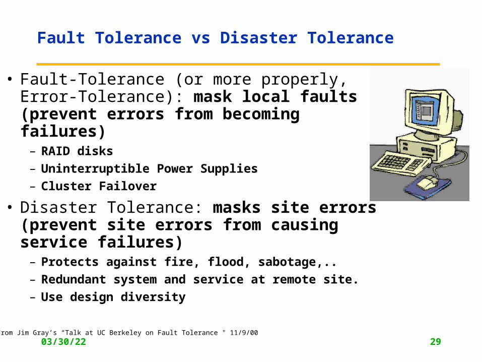
Fault Tolerance vs Disaster Tolerance

• Fault-Tolerance (or more properly, Error-Tolerance): mask local faults(prevent errors from becoming failures)

– RAID disks

– Uninterruptible Power Supplies

– Cluster Failover

• Disaster Tolerance: masks site errors(prevent site errors from causing service failures)

– Protects against fire, flood, sabotage,..

– Redundant system and service at remote site.

– Use design diversity

From Jim Gray’s “Talk at UC Berkeley on Fault Tolerance " 11/9/00

04/21/23 30

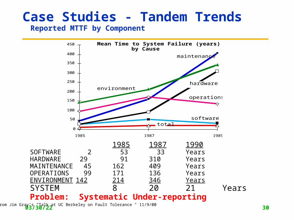
Case Studies - Tandem Trends Reported MTTF by Component

0

50

100

150

200

250

300

350

400

450

1985 1987 1989

software

hardware

maintenance

operations

environment

total

Mean Time to System Failure (years) by Cause

1985 1987 1990SOFTWARE 2 53 33 YearsHARDWARE 29 91 310 YearsMAINTENANCE 45 162 409 YearsOPERATIONS 99 171 136 YearsENVIRONMENT 142 214 346 YearsSYSTEM 8 20 21 YearsProblem: Systematic Under-reporting

From Jim Gray’s “Talk at UC Berkeley on Fault Tolerance " 11/9/00

04/21/23 31

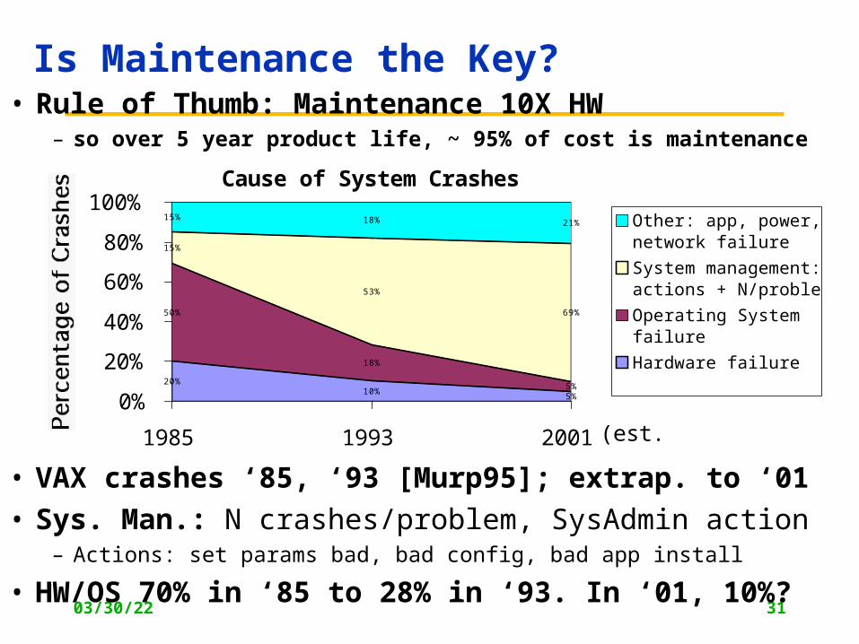
  Cause of System Crashes  

20%10%

5%

50%

18%

5%

15%

53%

69%

15% 18% 21%

0%

20%

40%

60%

80%

100%

1985 1993 2001

Other: app, power, network failure

System management: actions + N/problem

Operating Systemfailure

Hardware failure

(est.)

• VAX crashes ‘85, ‘93 [Murp95]; extrap. to ‘01

• Sys. Man.: N crashes/problem, SysAdmin action– Actions: set params bad, bad config, bad app install

• HW/OS 70% in ‘85 to 28% in ‘93. In ‘01, 10%?

• Rule of Thumb: Maintenance 10X HW– so over 5 year product life, ~ 95% of cost is maintenance

Is Maintenance the Key?

04/21/23 32

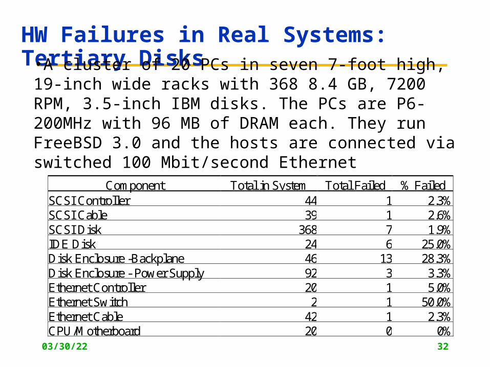
HW Failures in Real Systems: Tertiary Disks

Component Total in System Total Failed % FailedSCSI Controller 44 1 2.3%SCSI Cable 39 1 2.6%SCSI Disk 368 7 1.9%IDE Disk 24 6 25.0%Disk Enclosure -Backplane 46 13 28.3%Disk Enclosure - Power Supply 92 3 3.3%Ethernet Controller 20 1 5.0%Ethernet Switch 2 1 50.0%Ethernet Cable 42 1 2.3%CPU/Motherboard 20 0 0%

•A cluster of 20 PCs in seven 7-foot high, 19-inch wide racks with 368 8.4 GB, 7200 RPM, 3.5-inch IBM disks. The PCs are P6-200MHz with 96 MB of DRAM each. They run FreeBSD 3.0 and the hosts are connected via switched 100 Mbit/second Ethernet

04/21/23 33

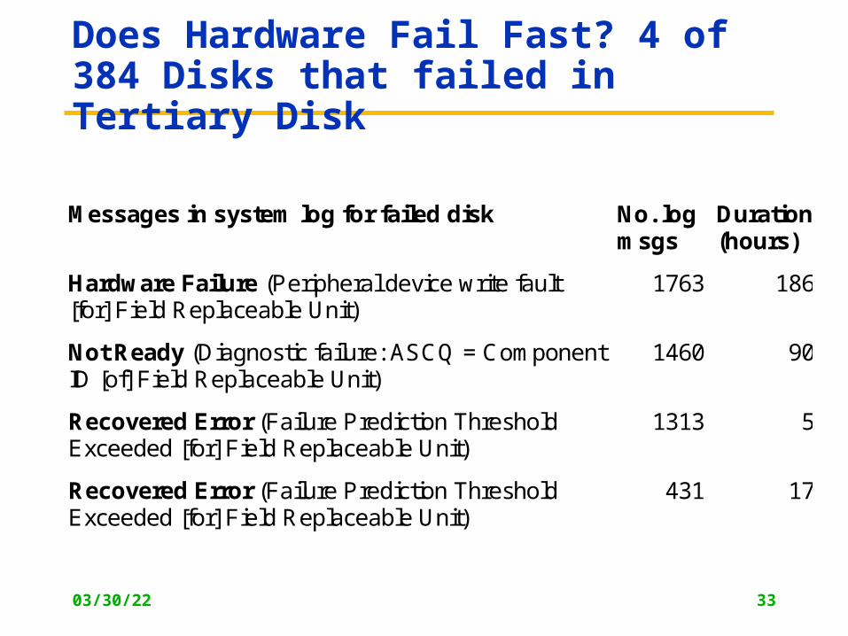
Does Hardware Fail Fast? 4 of 384 Disks that failed in Tertiary Disk

Messages in system log for failed disk No. log msgs

Duration (hours)

Hardware Failure (Peripheral device write fault [for] Field Replaceable Unit)

1763 186

Not Ready (Diagnostic failure: ASCQ = Component ID [of] Field Replaceable Unit)

1460 90

Recovered Error (Failure Prediction Threshold Exceeded [for] Field Replaceable Unit)

1313 5

Recovered Error (Failure Prediction Threshold Exceeded [for] Field Replaceable Unit)

431 17

04/21/23 34

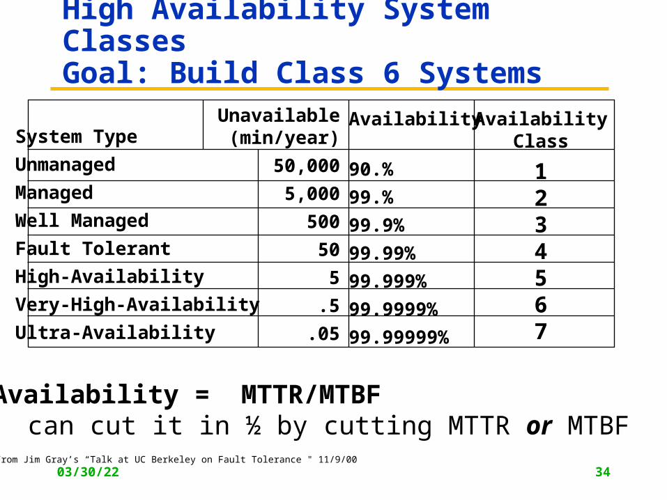
High Availability System ClassesGoal: Build Class 6 Systems

Availability

90.%

99.%

99.9%

99.99%

99.999%

99.9999%

99.99999%

System Type

Unmanaged

Managed

Well Managed

Fault Tolerant

High-Availability

Very-High-Availability

Ultra-Availability

Unavailable(min/year)

50,000

5,000

500

50

5

.5

.05

AvailabilityClass

1234567

UnAvailability = MTTR/MTBFcan cut it in ½ by cutting MTTR or MTBF

From Jim Gray’s “Talk at UC Berkeley on Fault Tolerance " 11/9/00

04/21/23 35

How Realistic is "5 Nines"?

• HP claims HP-9000 server HW and HP-UX OS can deliver 99.999% availability guarantee “in certain pre-defined, pre-tested customer environments”

– Application faults?

– Operator faults?

– Environmental faults?

• Collocation sites (lots of computers in 1 building on Internet) have

– 1 network outage per year (~1 day)

– 1 power failure per year (~1 day)

• Microsoft Network unavailable recently for a day due to problem in Domain Name Server: if only outage per year, 99.7% or 2 Nines

04/21/23 36

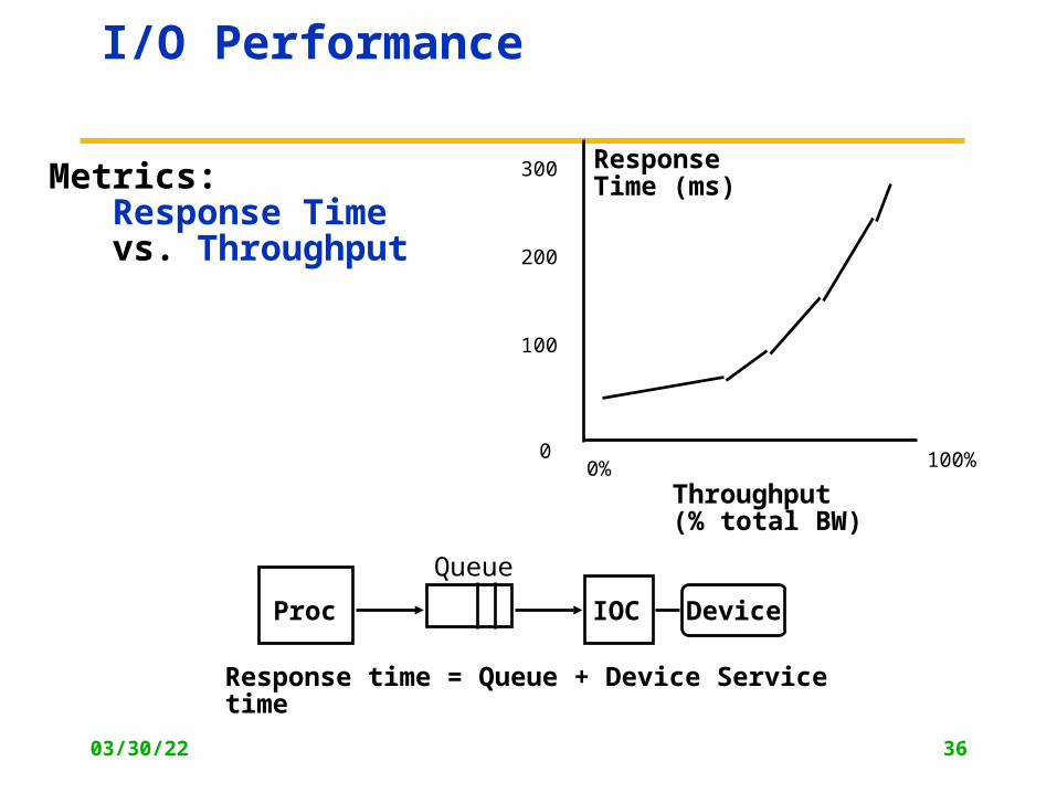
I/O Performance

Response time = Queue + Device Service time

100%

ResponseTime (ms)

Throughput (% total BW)

0

100

200

300

0%

Proc

Queue

IOC Device

Metrics: Response Time vs. Throughput

04/21/23 37

I/O Benchmarks

• For better or worse, benchmarks shape a field– Processor benchmarks classically aimed at response time for fixed

sized problem

– I/O benchmarks typically measure throughput, possibly with upper limit on response times (or 90% of response times)

• Transaction Processing (TP) (or On-line TP=OLTP)– If bank computer fails when customer withdraw money, TP system

guarantees account debited if customer gets $ & account unchanged if no $

– Airline reservation systems & banks use TP

• Atomic transactions makes this work

• Classic metric is Transactions Per Second (TPS)

04/21/23 38

Availability benchmark methodology

• Goal: quantify variation in QoS metrics as events occur that affect system availability

• Leverage existing performance benchmarks– to generate fair workloads– to measure & trace quality of service metrics

• Use fault injection to compromise system– hardware faults (disk, memory, network, power)– software faults (corrupt input, driver error returns)– maintenance events (repairs, SW/HW upgrades)

• Examine single-fault and multi-fault workloads– the availability analogues of performance micro- and macro-

benchmarks

04/21/23 39

Time (minutes)0 10 20 30 40 50 60 70 80 90 100 110

80

100

120

140

160

0

1

2

Hits/sec# failures tolerated

0 10 20 30 40 50 60 70 80 90 100 110

Hit

s p

er s

eco

nd

190

195

200

205

210

215

220

#fai

lure

s t

ole

rate

d

0

1

2

Reconstruction

Reconstruction

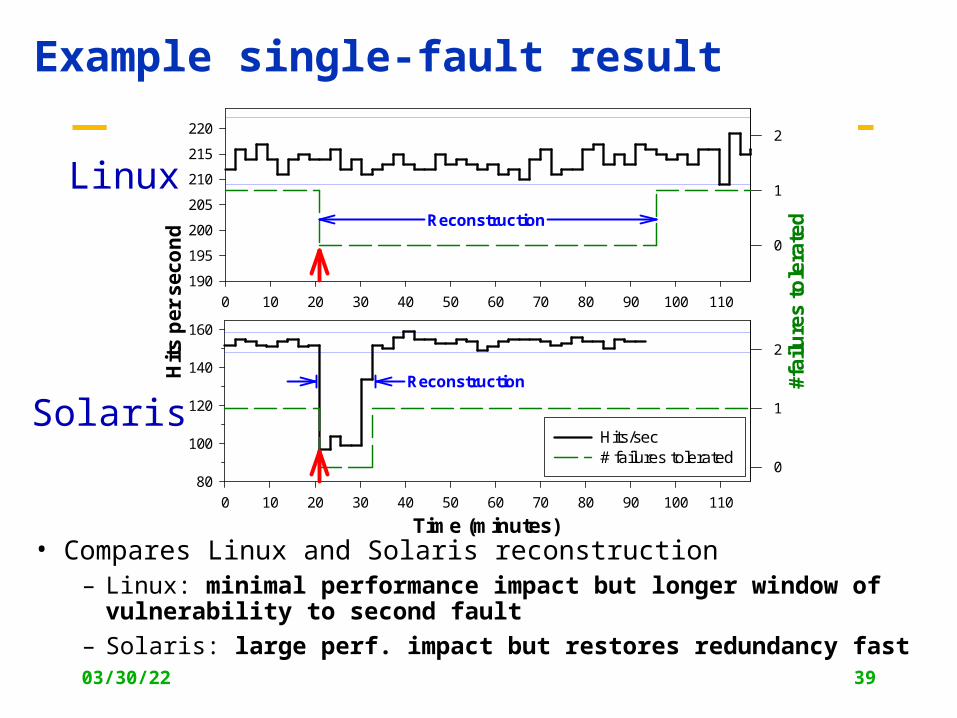
Example single-fault result

• Compares Linux and Solaris reconstruction– Linux: minimal performance impact but longer window of vulnerability

to second fault

– Solaris: large perf. impact but restores redundancy fast

Linux

Solaris

04/21/23 40

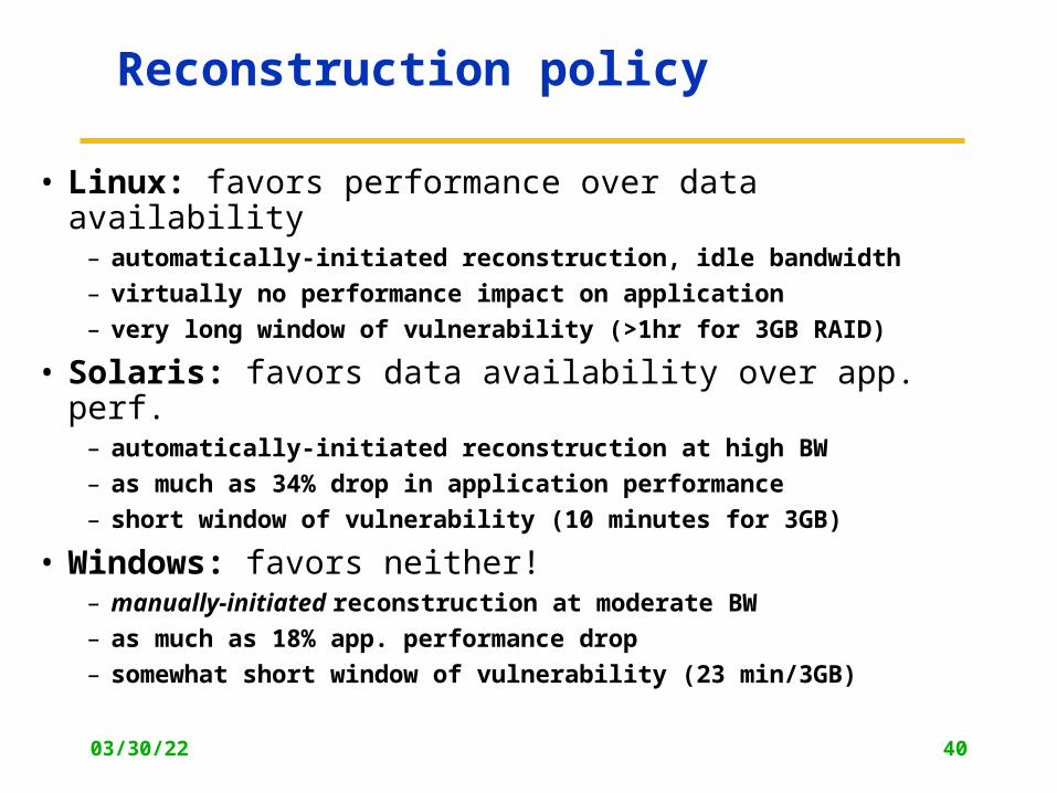
Reconstruction policy

• Linux: favors performance over data availability– automatically-initiated reconstruction, idle bandwidth

– virtually no performance impact on application

– very long window of vulnerability (>1hr for 3GB RAID)

• Solaris: favors data availability over app. perf.– automatically-initiated reconstruction at high BW

– as much as 34% drop in application performance

– short window of vulnerability (10 minutes for 3GB)

• Windows: favors neither!– manually-initiated reconstruction at moderate BW

– as much as 18% app. performance drop

– somewhat short window of vulnerability (23 min/3GB)

04/21/23 41

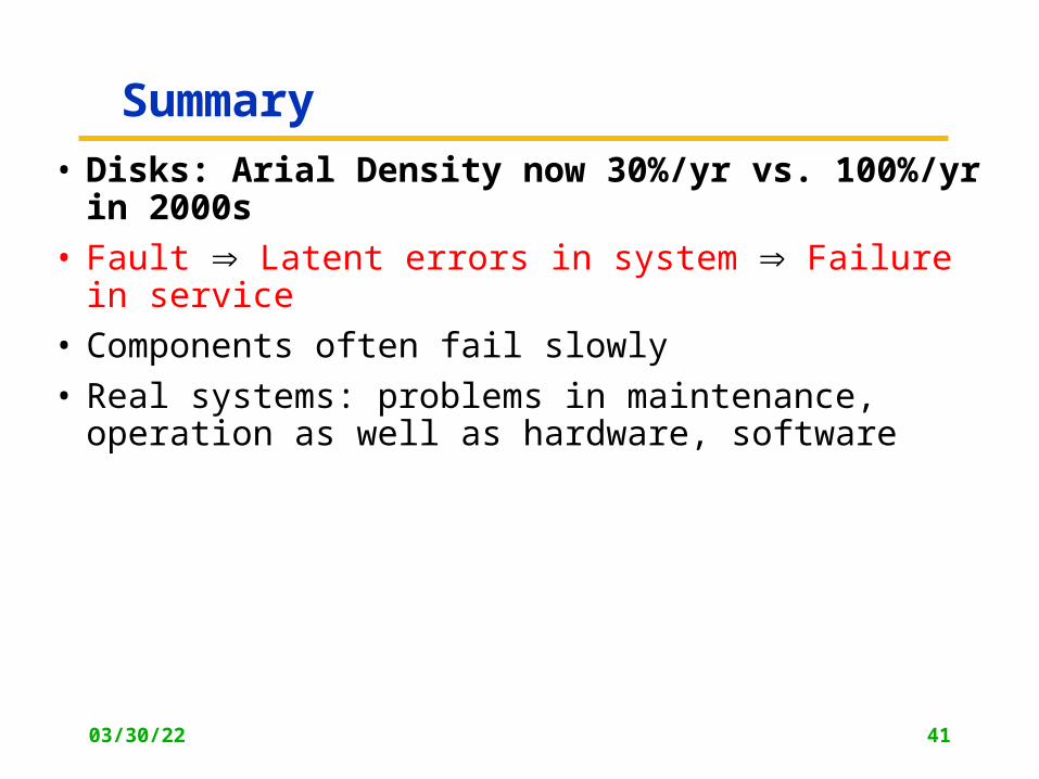
Summary• Disks: Arial Density now 30%/yr vs. 100%/yr in 2000s

• Fault Latent errors in system Failure in service

• Components often fail slowly

• Real systems: problems in maintenance, operation as well as hardware, software