Stochastic processes. Continuity and differentiability of ...roustant/Documents/Sample functions.pdf · Stochastic processes. Continuity and differentiability of sample functions

Introduction Sample functions properties in quadratic mean Sample functions properties References

Stochastic processes. Continuity anddifferentiability of sample functions

O. Roustant

École Nationale Supérieure des Mines de Saint-Étienne

12th of March 2009


Outline

1 Introduction

2 Sample functions properties in quadratic meanProcesses with finite second-order moments2nd order stationary processes

3 Sample functions propertiesSample function continuitySample function differentiability

4 References


INTRODUCTIONSAMPLE FUNCTIONS PROPERTIES


Example (from km.sim{DiceKriging})

0.0 1.0 2.0 3.0

0.00.2

0.40.6

0.81.0

distance

covariance

expmatern3_2matern5_2gauss

0.0 1.0 2.0 3.0

-2-1

01

2

input, x

outpu

t, f(x)


FIRST PARTSAMPLE FUNCTIONS PROPERTIES in QUADRATIC MEAN


Processes with finite second-order moments

Definitions and preliminary remarksLet Xt be a stochastic process.

Xt has finite second-order moments if ∀t , E(X 2t ) <∞

By Cauchy-Schwartz inequality this implies that∀u, v , E(Xu) and E(XuXv ) are well defined.As usual, L2 denotes the set of random variables with finitesecond order moments. Let us recall that L2 is a Hilbertspace, with < X , Y >= E(XY )

In the following, we will assume that E(Xt ) = 0 (if it not thecase, just consider Xt − E(Xt ))

We denote C(u, v) =< Xu, Xv > the covariance function.



Convergence in quadratic mean

DefinitionLet X1, X2, ..., Xn, ... and Y be r.v. with finite variances.Xn → Y in quadratic mean (q.m.) if ‖Xn − Y‖L2 → 0

Loeve criterionLet X1, X2, ..., Xn be n random variables with finite variances.Then Xn converges in q.m. iif < Xn, Xm > converges to a finitelimit c when n, m tend independently to infinity.

Proof hints.

For the "if" part, show that <, > is continuous.For the "iif" part, show that Xn is a Cauchy sequence.

Exercice. Find a counter example if n, m are not chosenindependently.



Continuity

Definition - Continuity in quadratic meanXt is continuous in q.m. at t = t0 if Xt → Xt0 in q.m.

Proposition1 Xt is continuous in q.m. at t = t0 iif the covariance function

C(u, v) is continuous at the diagonal point (t0, t0).2 If C(u, v) is continuous at every diagonal point (t , t), then it

is continuous everywhere.

Proof hints.1 For the "if" part, develop the expression E(Xt+h − Xt )

2

For the "iif" part, use the equality :C(t + h, t + k)− C(t , t) =< Xt+h − Xt , Xt+k − Xt >+ < Xt+h − Xt , Xt > + < Xt+k − Xt , Xt >

2 Use (1) and continuity of <, >.



Differentiability

Definition - Differentiability in quadratic mean

Xt is differentiable in q.m. at t if Xt+h−Xth converges in q.m.

Proposition

1 If ∂2C∂u∂v exists at (t , t), then Xt is differentiable in q.m. at t .

2 If ∂2C∂u∂v exists for every diagonal point (t , t), then ∂C

∂u (u, v)

and ∂2C∂u∂v (u, v) exist everywhere and we have :

cov(X ′u, Xv ) = ∂C∂u (u, v) and cov(X ′u, X ′v ) = ∂2C

∂u∂v (u, v)

Proof hint.1 Apply Loeve criterion to Yn =

Xt+hn−Xthn

for any seq. hn → 0.2 For the 1st derivative, use (1) and develop <

Xu+h−Xuh , Xv >.

Then develop <Xu+h−Xu

h ,Xv+k−Xv

k >.



Differentiability - Higher orders

Exercice

Show that if ∂4C∂u2∂v2 exists at (t , t), then Xt is diff. twice in q.m. at

t . In addition, if ∂4C∂u2∂v2 exists at every diagonal point, then all

derivatives written below exist everywhere and we have :

cov(X ′′u , Xv ) = ∂2C∂u2 (u, v)

cov(X ′′u , X ′v ) = ∂3C∂u2∂v (u, v)

cov(X ′′u , X ′′v ) = ∂4C∂u2∂v2 (u, v)

Generalize to any order.

Proof hint.For 2nd derivative existence, apply last proposition to X ′tand C′(u, v) := cov(X ′u, X ′v ).To prove the formulas, develop relevant expressions...


2nd order stationary processes


Definition

A stochastic process (Xt ) is 2nd order stationary if for any t , h,E(Xt ) and cov(Xt , Xt−h) do not depend on t .

Recall that we restrict to centered stochastic processes.Thus (Xt ) is stationary if C(u, v) is a function of u − v .We denote : C(h) = C(t , t − h).



Analytic properties of sample functions

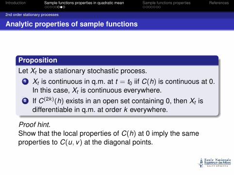
PropositionLet Xt be a stationary stochastic process.

1 Xt is continuous in q.m. at t = t0 iif C(h) is continuous at 0.In this case, Xt is continuous everywhere.

2 If C(2k)(h) exists in an open set containing 0, then Xt isdifferentiable in q.m. at order k everywhere.

Proof hint.Show that the local properties of C(h) at 0 imply the sameproperties to C(u, v) at the diagonal points.



A difficulty

Last results are easy to obtain. However :Continuity or differentiability in q.m. by no means necessarilyimplies sample function continuity or differentiability.


SECOND PARTSAMPLE FUNCTIONS PROPERTIES


A difficulty

Exercice 1Let Xt and Yt two stochastic processes defined over [0, 1] by :Xt (ω) = 0 ∀t , ωYt (ω) = 1 if t = ω and 0 otherwiseThen Xt and Yt have the same finite-dimensional distributionsbut :P({Xt is continuous in [0, 1]}) = 1P({Yt is continuous in [0, 1]}) = 0


A difficulty (following)

Exercice 2Let Xt and Yt two stochastic processes defined over [0, 1] by :Xt (ω) = 0 ∀t , ωYt (ω) = 1 if t =

1+ωn

n+1 and 0 otherwiseThen Xt and Yt have the same finite-dimensional distributions,but :P({Xt is continuous at 0}) = 1P({Yt is continuous at 0}) = 0


Equivalent processes

DefinitionWe say that Xt and Yt are equivalent if they have the samefinite dimensional distributions :

∀t , P({Xt = Yt}) = 1

Remarks.

This implies that two equivalent processes have the samefamily of finite-dimensional distributions.The examples above show that two equivalent processesdo NOT have the same sample functions properties.


Sample function continuity

Sample functions continuity - Kolmogorov theoremLet Xt be a stochastic process defined over [0, 1]. Suppose thatfor all t , t + h in [0, 1],

P({|Xt+h − Xt | ≥ g(h)}) ≤ q(h)

where g and q are even functions of h, non increasing as h ↓ 0,and such that

∞∑n=1

g(2−n) <∞ and∞∑

n=1

2nq(2−n) <∞.

Then there exists an equivalent stochastic process Yt whosesample functions are, with probability one, continuous on [0, 1].

Proof. See (Cramér, Leadbetter, 1967).



CorollaryIf with the notation above we have

E |Xt+h − Xt |p ≤K |h|

|log|h||1+r

where p < r and K are positive constants, the conclusion of thetheorem holds.

Proof. Apply Markov inequality : P(|X | ≥ a) ≤ |X |p

ap , and takeg(h) := |log|h||−b with 1 < b < r/p.



Stochastic processes with finite 2nd-order moments

Let Xt be a stochastic process with finite 2nd order moments. Iffor all t and t + h in [a, b] the difference

∆2hC(t , t) := C(t + h, t + h)− C(t + h, t)− C(t , t + h)− C(t , t)

satisfies an inequality of the form ∆2hC(t , t) < K |h|

|log|h||q , withq > 3 and K > 0, then Xt is equivalent to a stochastic processwhich, with probability one, is sample continuous.

Stationary processesLet Xt be a stationary stochastic process. If C′′(0) exists, thenXt is equivalent to a stochastic process which, with probabilityone, is sample continuous.

Proof. Apply corollary with p = 2.


Sample function differentiability

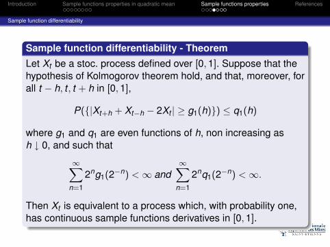
Sample function differentiability - TheoremLet Xt be a stoc. process defined over [0, 1]. Suppose that thehypothesis of Kolmogorov theorem hold, and that, moreover, forall t − h, t , t + h in [0, 1],

P({|Xt+h + Xt−h − 2Xt | ≥ g1(h)}) ≤ q1(h)

where g1 and q1 are even functions of h, non increasing ash ↓ 0, and such that

∞∑n=1

2ng1(2−n) <∞ and∞∑

n=1

2nq1(2−n) <∞.

Then Xt is equivalent to a process which, with probability one,has continuous sample functions derivatives in [0, 1].



CorollaryIf the conditions of Kolmogorov theorem’s corollary are satisfiedand if, moreover

E |Xt+h + Xt−h − 2Xt |p ≤K |h|1+p

|log|h||1+r

where p < r and K are positive constants, the conclusion of thetheorem holds.

Proofs. For the theorem, see (Cramér, Leadbetter, 1967). Forthe corollary, apply again Markov inequality.



Stochastic processes with finite 2nd-order moments

Let Xt be a stochastic process with finite 2nd order moments. Iffor all t , h the fourth difference ∆4

hC(t , t) satisfies an inequality

of the form ∆4hC(t , t) < K |h|3

|log|h||q , with q > 3 and K > 0, then Xt isequivalent to a process which, with probability one, hascontinuous sample function derivatives.

Stationary processes

Let Xt be a stationary stochastic process. If C(4)(0) exists, thenXt is equivalent to a process which, with probability one, issample continuous.

Proof. Again appply corollary with p = 2.



Differentiability - Higher ordersThere are analogous results. In particular, if Xt is a stationarystochastic process and if C(2k+2)(0) exists, then Xt isequivalent to a process which, with probability one, has Ck

sample functions.


REFERENCES


ReferencesCramér H., Leadbetter M.R. (1967), Stationary andRelated Stochastic Processes - Sample FunctionProperties and Their Applications, Wiley.Rasmussen C.E., Williams C.K.I. (2006), GaussianProcesses for Machine Learning, the MIT Press.