Stochastic Expansions in an OvercompleteWavelet Dictionary

F. Abramovich, T. Sapatinas and B. W. Silverman

Tel Aviv University, University of Kent at Canterbury, University of Bristol.

2 July 1999

Abstract

We consider random functions defined in terms of members of an overcompletewavelet dictionary. The function is modelled as a sum of wavelet componentsat arbitrary positions and scales where the locations of the wavelet componentsand the magnitudes of their coefficients are chosen with respect to a marked Pois-son process model. The relationships between the parameters of the model andthe parameters of those Besov spaces within which realizations will fall are in-vestigated. The models allow functions with specified regularity properties tobe generated. They can potentially be used as priors in a Bayesian approach tocurve estimation, extending current standard wavelet methods to be free from thedyadic positions and scales of the basis functions.

Keywords: BESOV SPACES; CONTINUOUS WAVELET TRANSFORM; OVER-COMPLETE WAVELET DICTIONARIES; POISSON PROCESSES.

1 Introduction

1.1 Background

Wavelets have recently been of great interest in various statistical areas such as non-parametric regression, density estimation, inverse problems, change point problems,and time series analysis. Surveys of wavelet applications in these and other related

Address for correspondence: Institute of Mathematics and Statistics, University of Kent at Canter-bury, Canterbury, Kent CT2 7NF, United Kingdom. Email: T.Sapatinas@ukc.ac.uk

1

statistical areas can be found, for example, in Ogden (1997), Hardle, Kerkyachar-ian, Picard & Tsybakov (1998), Abramovich, Bailey & Sapatinas (1999), Antoniadis(1999), Silverman (1999) and Vidakovic (1999). An interesting development, moti-vated by Bayesian approaches to curve estimation, is the modelling of a function as anorthonormal wavelet expansion with random coefficients. Abramovich, Sapatinas &Silverman (1998) considered such models in detail, and studied the Besov regularityproperties of the functions produced by the models. They consider the application ofthe models in a Bayesian context, and also give references to related work by otherauthors; the results obtained have generally been very encouraging.

1.2 Abandoning dyadic constraints

Orthonormal wavelet bases have the disadvantage that the positions and the scales ofthe basis functions are subject to dyadic constraints. In order to avoid these constraints,this paper considers random functions defined by expansions in a continuous waveletdictionary, where functions are built up from wavelet components that may have ar-bitrary positions and scales. The models provide a constructive method of simulatingfunctions with varying degrees of regularity and spatial homogeneity, and our resultsgive the explicit regularity properties of the functions thus produced, in terms of Besovspaces.

Some users might wish to be able to simulate or construct functions with specificBesov parameters in mind. Others might wish to use the models to gain intuition aboutthe meaning of the Besov parameters, by generating functions that lie just inside andjust outside particular Besov spaces. The models lay open the possibility of buildinga Bayesian curve estimation approach with the advantages of standard wavelet meth-ods, in that inhomogeneous functions can be modelled under the prior, but withoutthe artificial dyadic constraints on the positions and scales of the basis functions. Theimprovement to standard wavelet thresholding methods obtained by moving from thediscrete (decimated) wavelet transform to the non-decimated wavelet transform (see,for example, Coifman & Donoho, 1995; Nason & Silverman, 1995; Johnstone & Sil-verman, 1997) suggests that a Bayesian approach freed from dyadic positions andscales may result in yet better wavelet shrinkage estimators. The algorithmic details,probably involving modern Bayesian computational methods, have yet to be workedout in detail, and this is an interesting topic for further research.

1.3 Models in continuous wavelet dictionaries

For simplicity of exposition we work with functions periodic on . Suppose thatand are the compact-support scaling function and mother wavelet respectively thatcorrespond to an -regular multiresolution analysis, for some integer (see, forexample, Daubechies, 1992). Take , for some integer , such that is at least

2

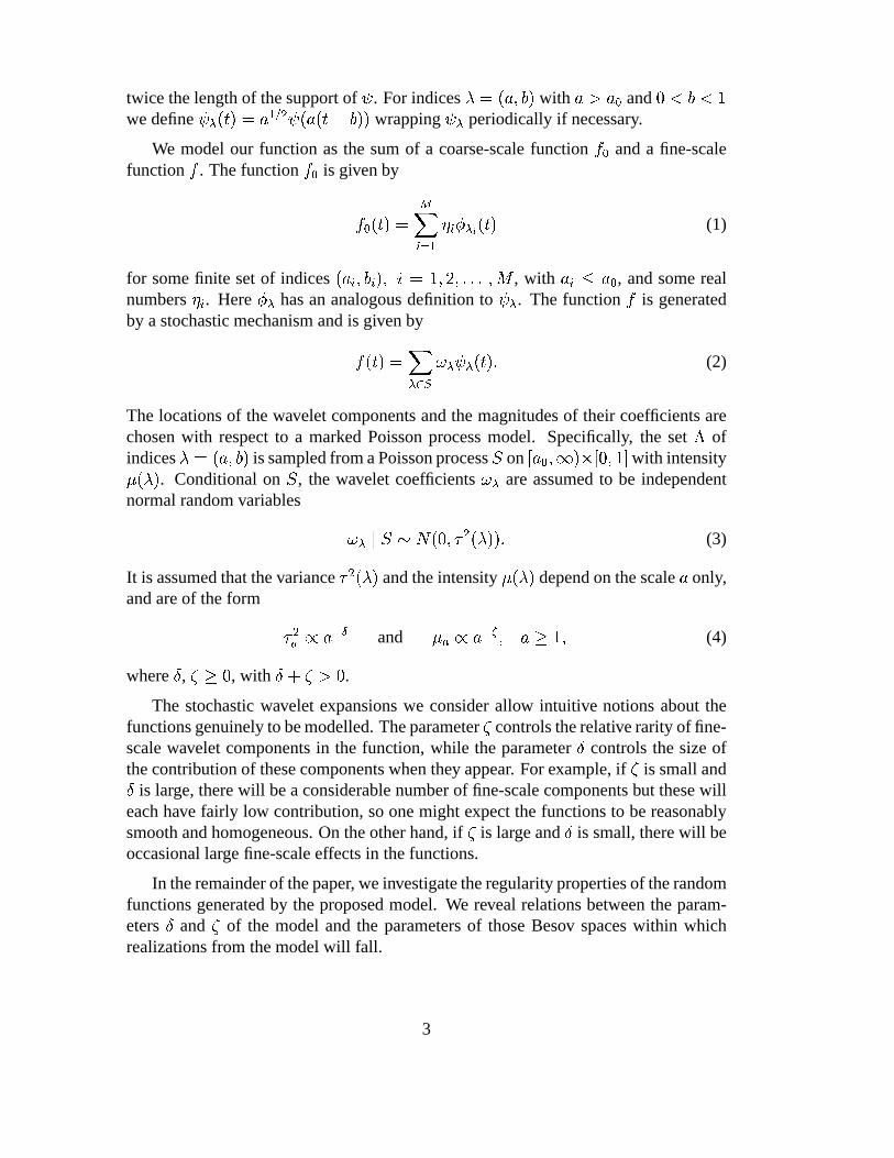
twice the length of the support of . For indices with andwe define wrapping periodically if necessary.

We model our function as the sum of a coarse-scale function and a fine-scalefunction . The function is given by

(1)

for some finite set of indices , with , and some realnumbers . Here has an analogous definition to . The function is generatedby a stochastic mechanism and is given by

(2)

The locations of the wavelet components and the magnitudes of their coefficients arechosen with respect to a marked Poisson process model. Specifically, the set ofindices is sampled from a Poisson process on with intensity

. Conditional on , the wavelet coefficients are assumed to be independentnormal random variables

(3)

It is assumed that the variance and the intensity depend on the scale only,and are of the form

and (4)

where , , with .

The stochastic wavelet expansions we consider allow intuitive notions about thefunctions genuinely to be modelled. The parameter controls the relative rarity of fine-scale wavelet components in the function, while the parameter controls the size ofthe contribution of these components when they appear. For example, if is small and

is large, there will be a considerable number of fine-scale components but these willeach have fairly low contribution, so one might expect the functions to be reasonablysmooth and homogeneous. On the other hand, if is large and is small, there will beoccasional large fine-scale effects in the functions.

In the remainder of the paper, we investigate the regularity properties of the randomfunctions generated by the proposed model. We reveal relations between the param-eters and of the model and the parameters of those Besov spaces within whichrealizations from the model will fall.

3

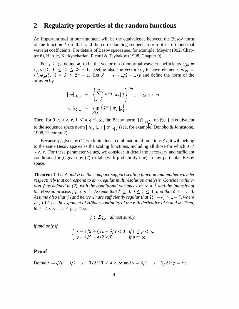
2 Regularity properties of the random functions

An important tool in our argument will be the equivalence between the Besov normof the function on and the corresponding sequence norm of its orthonormalwavelet coefficients. For details of Besov spaces see, for example, Meyer (1992, Chap-ter 6), Hardle, Kerkyacharian, Picard & Tsybakov (1998, Chapter 9).

For , define to be the vector of orthonormal wavelet coefficients. Define also the vector to have elements. Let and define the norm of the

array by

Then, for , , the Besov norm on is equivalent

to the sequence space norm (see, for example, Donoho & Johnstone,1998, Theorem 2)

Because given by (1) is a finite linear combination of functions , it will belongto the same Besov spaces as the scaling functions, including all those for which

. For these parameter values, we consider in detail the necessary and sufficientconditions for given by (2) to fall (with probability one) in any particular Besovspace.

Theorem 1 Let and be the compact-support scaling function and mother waveletrespectively that correspond to an -regular multiresolution analysis. Consider a func-tion as defined in (2), with the conditional variances and the intensity ofthe Poisson process . Assume that , , and thatAssume also that (and hence ) are sufficiently regular that , where

is the exponent of Holder continuity of the -th derivative of and . Then,for ,

almost surely

if and only ififif

Proof

Define if and if .

4

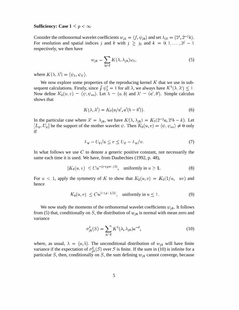
Sufficiency: Case

Consider the orthonormal wavelet coefficients and set .For resolution and spatial indices and with andrespectively, we then have

(5)

where

We now explore some properties of the reproducing kernel that we use in sub-sequent calculations. Firstly, since for all , we always haveNow define Let and . Simple calculusshows that

(6)

In the particular case where , we have . Letbe the support of the mother wavelet . Then only

if

(7)

In what follows we use to denote a generic positive constant, not necessarily thesame each time it is used. We have, from Daubechies (1992, p. 48),

uniformly in (8)

For , apply the symmetry of to show that andhence

uniformly in (9)

We now study the moments of the orthonormal wavelet coefficients . It followsfrom (5) that, conditionally on , the distribution of is normal with mean zero andvariance

(10)

where, as usual, The unconditional distribution of will have finitevariance if the expectation of over is finite. If the sum in (10) is infinite for aparticular , then, conditionally on , the sum defining cannot converge, because

5

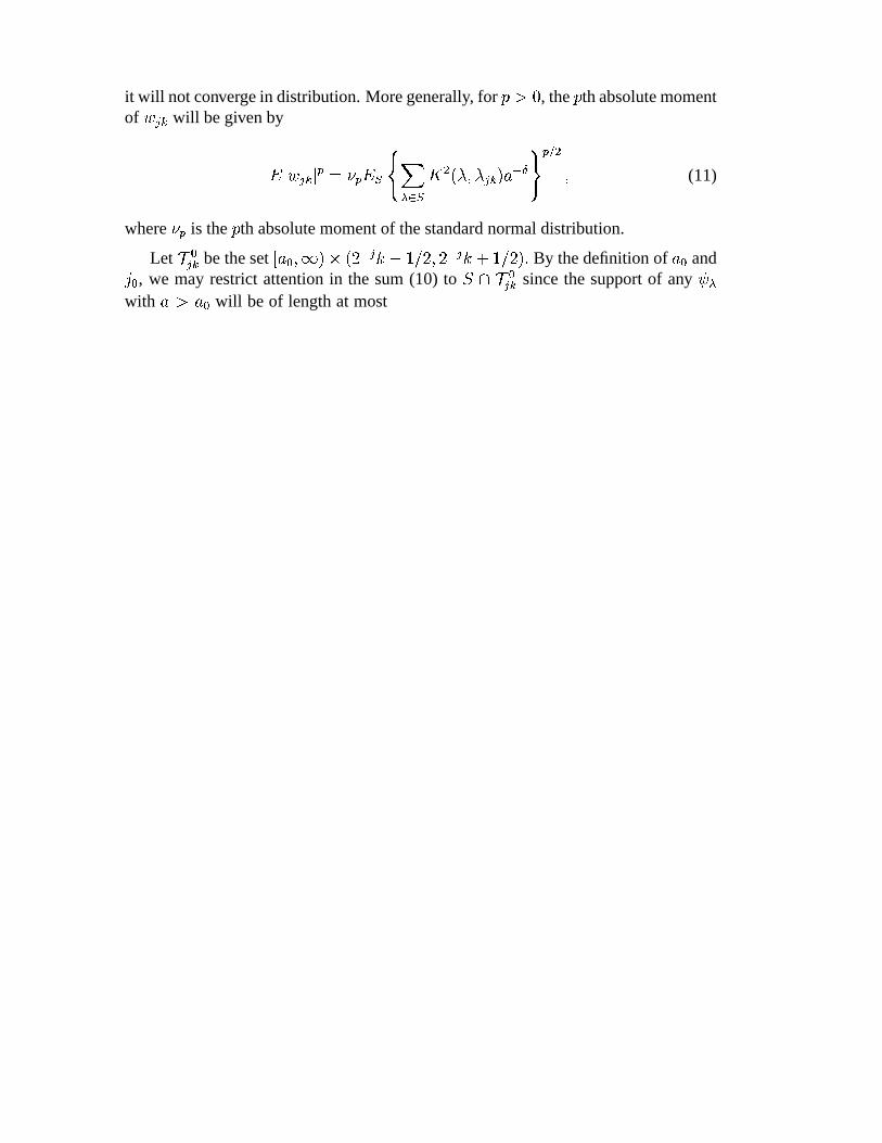
it will not converge in distribution. More generally, for , the th absolute momentof will be given by

(11)

where is the th absolute moment of the standard normal distribution.

Let be the set By the definition of and, we may restrict attention in the sum (10) to since the support of any

with will be of length at most , and so the terms excluded by restricting thesum will all be zero. Now let be a Poisson process on the half-plane

of intensity . Define the setConsider the transformation of given by . Appliedto the process this gives a process with the same distribution as Inaddition, for each , we have from (6) that It follows that

(12)

To obtain a bound on the expectation in (12), define the random sum

(13)

The bounds (8) and (9) imply that is bounded by for, and by for hence it is uniformly bounded for all and .

We now apply Corollary 1 in the Appendix to investigate the behaviour of .To verify the finiteness of the first integral in the corollary, it will be sufficient to havefiniteness of the integral

(14)

The bounds (7) on the support of the integrand, and those stated above on its order ofmagnitude, allow (14) to be dominated by

6

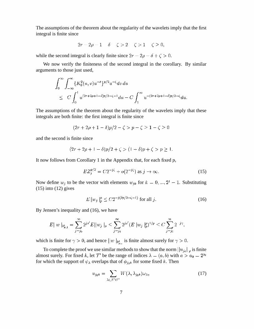
The assumptions of the theorem about the regularity of the wavelets imply that the firstintegral is finite since

while the second integral is clearly finite since .

We now verify the finiteness of the second integral in the corollary. By similararguments to those just used,

The assumptions of the theorem about the regularity of the wavelets imply that theseintegrals are both finite: the first integral is finite since

and the second is finite since

It now follows from Corollary 1 in the Appendix that, for each fixed ,

as (15)

Now define to be the vector with elements for . Substituting(15) into (12) gives

for all . (16)

By Jensen’s inequality and (16), we have

which is finite for , and hence is finite almost surely for .

To complete the proof we use similar methods to show that the norm is finitealmost surely. For fixed , let be the range of indices withfor which the support of overlaps that of for some fixed . Then

(17)

7

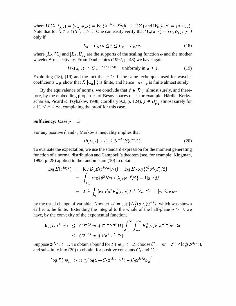
where and .Note that for , . One can easily verify thatonly if

(18)

where and are the supports of the scaling function and the motherwavelet respectively. From Daubechies (1992, p. 48) we have again

uniformly in (19)

Exploiting (18), (19) and the fact that , the same techniques used for waveletcoefficients show that is finite, and hence is finite almost surely.

By the equivalence of norms, we conclude that almost surely, and there-fore, by the embedding properties of Besov spaces (see, for example, Hardle, Kerky-acharian, Picard & Tsybakov, 1998, Corollary 9.2, p. 124), almost surely forall , completing the proof for this case.

Sufficiency: Case

For any positive and , Markov’s inequality implies that

(20)

To evaluate the expectation, we use the standard expression for the moment generatingfunction of a normal distribution and Campbell’s theorem (see, for example, Kingman,1993, p. 28) applied to the random sum (10) to obtain

by the usual change of variable. Now let , which was shownearlier to be finite. Extending the integral to the whole of the half-plane , wehave, by the convexity of the exponential function,

Suppose . To obtain a bound for , choose ,and substitute into (20) to obtain, for positive constants and ,

8

Both and are positive by the hypotheses of the theorem. Choose suchthat and set . Then We now have

for sufficiently large . Since is of length , it follows that, for sufficiently large ,

This very rapidly decreasing bound on the tail probabilities implies that, with probabil-ity one, the sequence is bounded by a multiple of , and henceis finite almost surely. The same arguments used in the case of finite for scalingcoefficients show that is finite almost surely.

By the equivalence of norms, we conclude that almost surely and, there-fore, by the embedding properties of Besov spaces (see, for example, Hardle, Kerky-acharian, Picard & Tsybakov, 1998, Corollary 9.2, p. 124), almost surely forall , completing the proof for this case, and hence we have the sufficiency.

Necessity

Noting that the function is continuous and that , choose withsuch that for all with and .

For and , define the nonoverlapping rectangles in therange of indices as .

Using (4), the expected number of wavelet components falling within is thenfor some , and hence the probability that there is one or

more wavelet components in is at least for some . Now define

and observe that the are independent because the are disjoint. It follows from(6) that for in . Note also that from (3) and (4), Var

for some , so that Var .

For and , now define independent random variablesto have the mixture distribution

where and . For the orthonormal wavelet coefficients, it is obvious that is stochastically larger than which in turn is

9

stochastically larger than . Hence, stochasticallyfor any , .

The methods of Abramovich, Sapatinas & Silverman (1998) for independent or-thonormal wavelet coefficients (see their Theorem 1) now show that if isfinite almost surely, then . This completes the proof of necessity, and hence thatof the theorem as a whole.

3 Concluding remarks

Theorem 1 places an upper bound restriction on the value of . In the case ,the intensity is integrable over the range of for which has supportintersecting . Therefore, the number of relevant terms in the stochastic expansionof is finite almost surely. With probability one, will belong to the same Besovspaces as the mother wavelet , namely those for which , ,

.

The key conclusion of Theorem 1 we have proved is that, under suitable condi-tions, the function falls in if exceeds . Since the fine-scalecontent of model functions depends both on the intensity of fine-scale components andon their size, it is not surprising that the smoothness as measured by the parameter

should depend on both parameters. The parameter can be seen as discouraginginhomogeneity, in that the larger the value of the more emphasis is placed on theparameter . For large , no matter how many fine-scale components there are, theyeach make a relatively low contribution. On the other hand, if is small, then there isa trade-off where large weights on fine-scale components (small ) can be tolerated ifthe corresponding components are relatively rare (large ).

The constraints placed on in the statistical literature, for example in the optimalityresults of Donoho & Johnstone (1998), are often stronger than those we have assumed.Typical conditions are or . These constraintsensure that the Besov spaces are function spaces rather than spaces of more generaldistributions (see, for example, Meyer, 1992, Chapter 6).

Acknowledgements

We are delighted to thank Boris Tsirelson for fruitful discussions. The financial sup-port of the Engineering and Physical Sciences Research Council, the Israel Academyof Science, and the Royal Society are gratefully acknowledged. During periods ofthe work TS was a Research Associate in the School of Mathematics, University ofBristol, supported by EPSRC grant GR/K70236, and BWS was a Fellow at the Centerfor Advanced Study in the Behavioral Sciences, Stanford, partly supported by NSF

10

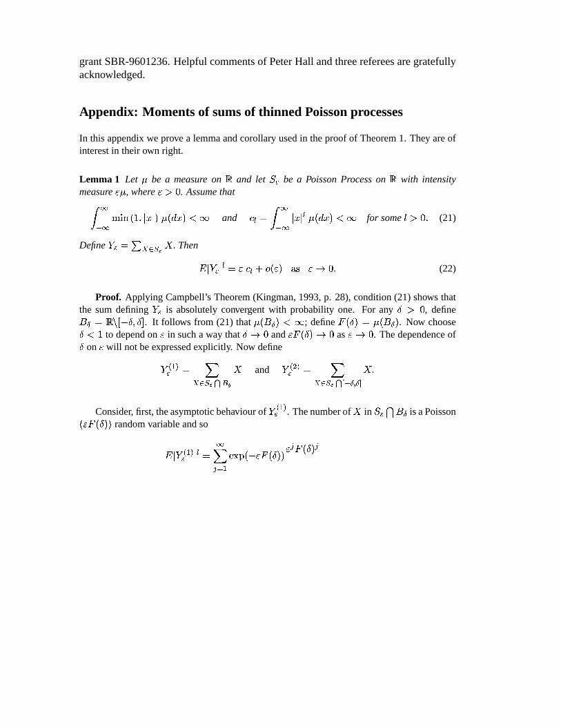
grant SBR-9601236. Helpful comments of Peter Hall and three referees are gratefullyacknowledged.

Appendix: Moments of sums of thinned Poisson processes

In this appendix we prove a lemma and corollary used in the proof of Theorem 1. They are ofinterest in their own right.

Lemma 1 Let be a measure on and let be a Poisson Process on with intensitymeasure , where . Assume that

and for some (21)

Define Then

(22)

Proof. Applying Campbell’s Theorem (Kingman, 1993, p. 28), condition (21) shows thatthe sum defining is absolutely convergent with probability one. For any , define

. It follows from (21) that ; define . Now chooseto depend on in such a way that and as . The dependence of

on will not be expressed explicitly. Now define

and

Consider, first, the asymptotic behaviour of . The number of in is a Poissonrandom variable and so

(23)

where are independent and identically distributed random variables on withdistribution . Let . For , we consider a bound for theexpectation in (23). For , we immediately see that

(24)

For , using Jensen’s inequality, we have

(25)

11

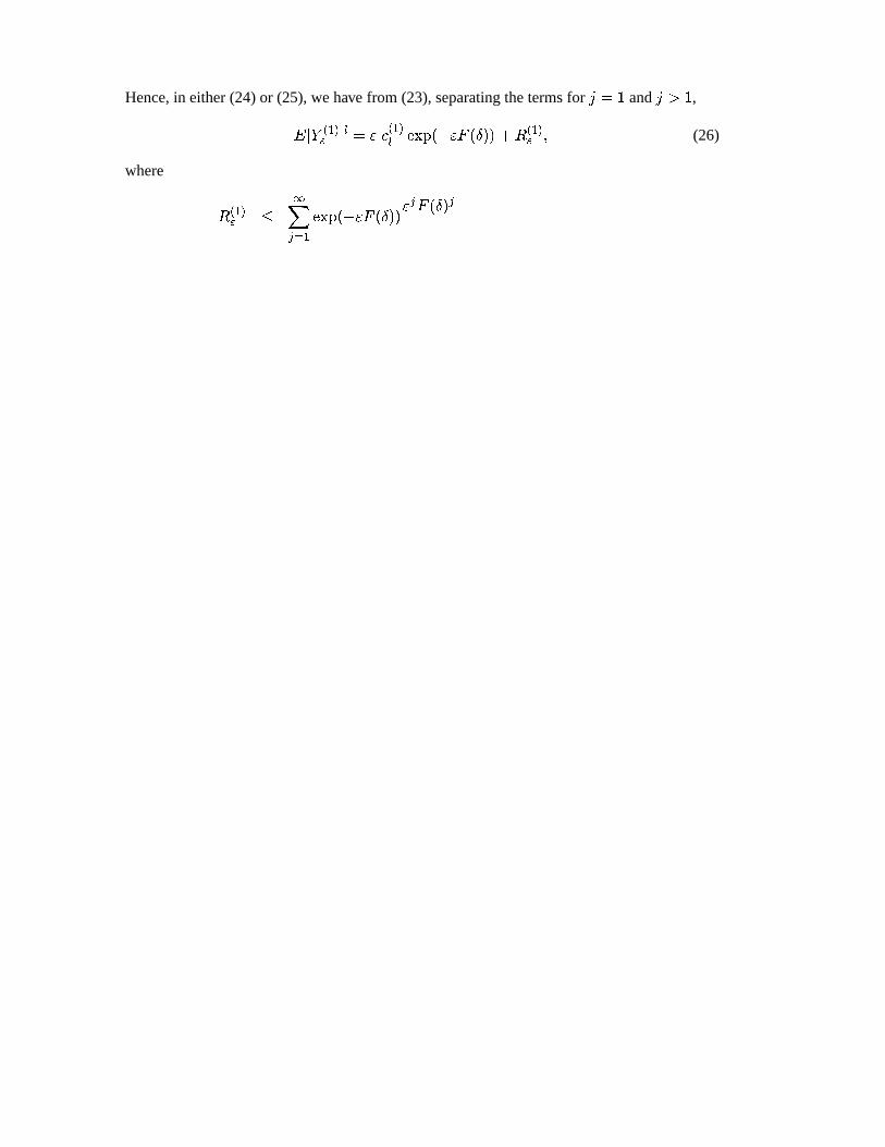
Hence, in either (24) or (25), we have from (23), separating the terms for and ,

(26)

where

(27)

As , the sum in (27) is a Poisson expectation that converges to , since .

It follows that and hence, from (26), that, as :

(28)

using the facts that and .

Now consider the asymptotic behaviour of . For , by Campbell’s theorem appliedto the Poisson process , we have

(29)

Therefore, we have from (29), as , that . Sinceit follows from (28) that as

Finally, consider the case . Define . For , we

have , and so, using (21), It thenfollows (using equation (3.17) of Kingman, 1993), that Since ,there exists a constant such that for all . We then have

as (30)

since as . Therefore, from (30), it follows at once that as

Using Minkowski’s inequality applied to the norm we have:

and hence, since , the limiting values of and are thesame. It follows from (28) that , which gives (22), completing the proof of thelemma.

12

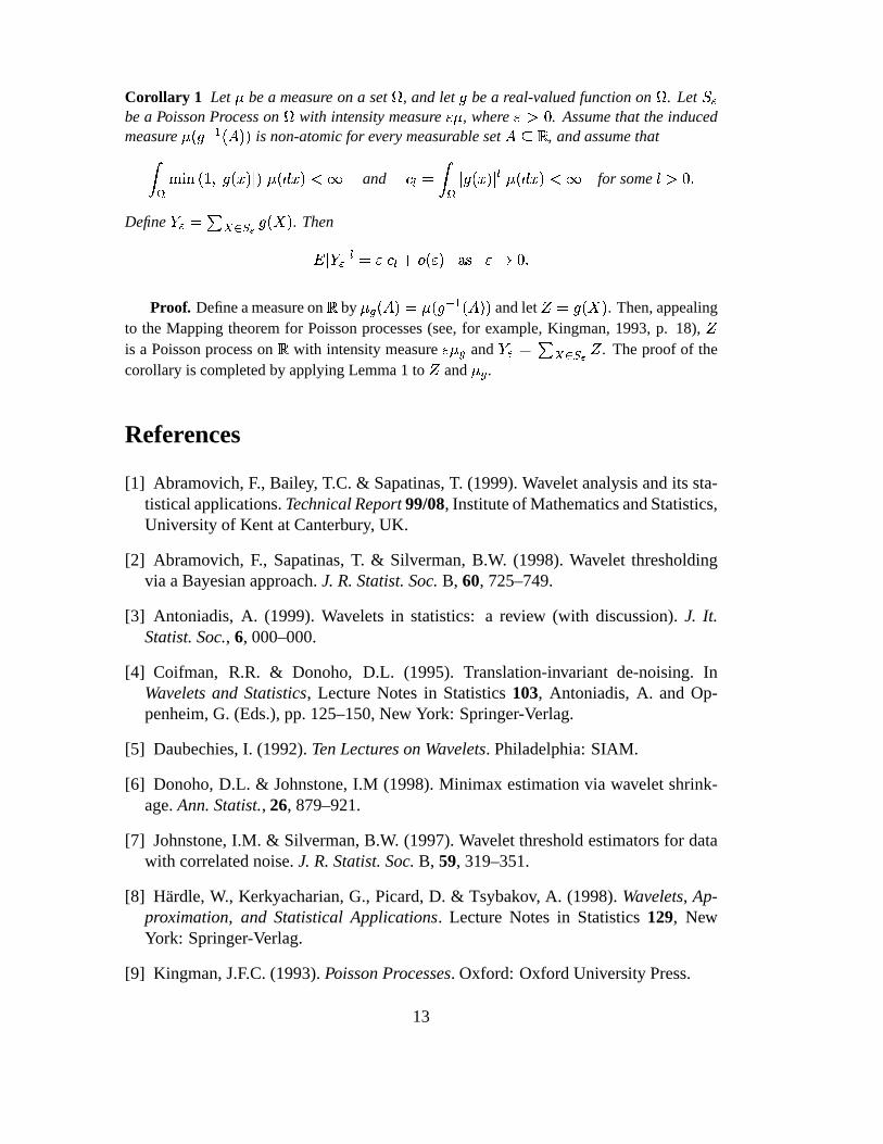
Corollary 1 Let be a measure on a set , and let be a real-valued function on . Letbe a Poisson Process on with intensity measure , where . Assume that the inducedmeasure is non-atomic for every measurable set , and assume that

and for some

Define . Then

Proof. Define a measure on by and let . Then, appealingto the Mapping theorem for Poisson processes (see, for example, Kingman, 1993, p. 18),is a Poisson process on with intensity measure and . The proof of thecorollary is completed by applying Lemma 1 to and .

References

[1] Abramovich, F., Bailey, T.C. & Sapatinas, T. (1999). Wavelet analysis and its sta-tistical applications. Technical Report 99/08, Institute of Mathematics and Statistics,University of Kent at Canterbury, UK.

[2] Abramovich, F., Sapatinas, T. & Silverman, B.W. (1998). Wavelet thresholdingvia a Bayesian approach. J. R. Statist. Soc. B, 60, 725–749.

[3] Antoniadis, A. (1999). Wavelets in statistics: a review (with discussion). J. It.Statist. Soc., 6, 000–000.

[4] Coifman, R.R. & Donoho, D.L. (1995). Translation-invariant de-noising. InWavelets and Statistics, Lecture Notes in Statistics 103, Antoniadis, A. and Op-penheim, G. (Eds.), pp. 125–150, New York: Springer-Verlag.

[5] Daubechies, I. (1992). Ten Lectures on Wavelets. Philadelphia: SIAM.

[6] Donoho, D.L. & Johnstone, I.M (1998). Minimax estimation via wavelet shrink-age. Ann. Statist., 26, 879–921.

[7] Johnstone, I.M. & Silverman, B.W. (1997). Wavelet threshold estimators for datawith correlated noise. J. R. Statist. Soc. B, 59, 319–351.

[8] Hardle, W., Kerkyacharian, G., Picard, D. & Tsybakov, A. (1998). Wavelets, Ap-proximation, and Statistical Applications. Lecture Notes in Statistics 129, NewYork: Springer-Verlag.

[9] Kingman, J.F.C. (1993). Poisson Processes. Oxford: Oxford University Press.

13

[10] Meyer, Y. (1992). Wavelets and Operators. Cambridge: Cambridge UniversityPress.

[11] Nason, G.P. & Silverman, B.W. (1995). The stationary wavelet transform andsome statistical applications. In Wavelets and Statistics, Lecture Notes in Statistics103, Antoniadis, A. and Oppenheim, G. (Eds.), pp. 281-300, New York: Springer-Verlag.

[12] Ogden, T.R. (1997). Essential Wavelets for Statistical Applications and DataAnalysis. Boston: Birkhauser.

[13] Silverman, B.W. (1999). Wavelets in statistics: beyond the standard assumptions.Phil. Trans. Roy. Soc. Lond. A, 357, 000–000.

[14] Vidakovic, B. (1999). Statistical Modeling by Wavelets. New York: John Wiley& Sons.

14