Embed Size (px)
DESCRIPTION
mathematics
Citation preview
Chapter 7
The Stirling Numbersof the Second Kind
7.1. Introduction
This chapter considers the Stirling numbers of the second kind
with special emphasis on their arithmetic properties. The other kind
of Stirling numbers, those of the first kind, are not considered here.
Definition 7.1.1. Let n, k ≥ 1. The Stirling numbers of the
second kind S(n, k) count the ways to divide a set of n objects into
k nonempty subsets.
Note 7.1.2. From the definition it is clear that S(n, k) = 0 if n < k.
The extension
S(0, k) =
{1 if k = 0,
0 if k > 0
defines S(0, k).
Example 7.1.3. The number S(n, 1) = 1 since the only option is
to place all the objects into the single subset. Similarly, S(n, n) = 1
since then you must place each object in a different subset.
191
192 7. The Stirling Numbers of the Second Kind
Example 7.1.4. The list
{{1, 2, 3}, {4}}, {{1, 2, 4}, {3}}, {{1, 3, 4}, {2}}, {{2, 3, 4}, {1}},
{{1, 2}, {3, 4}}, {{1, 3}, {2, 4}}, {{1, 4}, {2, 3}}shows that S(4, 2) = 7.
Exercise 7.1.5. Give a combinatorial proof of the value
(7.1.1) S(n, n− 1) =
(n
2
).
Exercise 7.1.6. Prove that
(7.1.2) S(n, 2) = 2n−1 − 1.
7.2. A recurrence
In the partition of {1, 2, . . . , n} into k nonempty subsets, there are
cases in which n appears as a singleton and others in which n is
part of one of the k nonempty subsets with more than one element.
In the first case, the partition is {n} together with a partition of
{1, 2, . . . , n−1} into k−1 nonempty parts. There are S(n−1, k−1)
of them. In the second case, taking n out of the partition yields a
collection of k nonempty subsets partitioning {1, 2, . . . , n−1}. There
are S(n− 1, k) of them. The number n can be placed back into any
of the k parts. This proves the next result.
Theorem 7.2.1. The Stirling numbers of the second kind satisfy the
recurrence
(7.2.1) S(n, k) = S(n− 1, k − 1) + kS(n− 1, k)
for n ≥ 2.
Exercise 7.2.2. The theorem and S(n, 1) = n state that
(7.2.2) S(n, 2) − 2S(n− 1, 2) = S(n− 1, 1) = 1.
Solve this recurrence to confirm the value S(n, 2) = 2n−1−1 stated in
Exercise 7.1.6. Discuss the consistency of the value S(0, k) and this
recurrence.
7.2. A recurrence 193
Exercise 7.2.3. Let f(x) = 1/(1 + ex). Prove that
(7.2.3) f (n)(x) =
n+1∑k=1
a(n, k)
(1 + ex)k
where
(7.2.4) a(n, k) = (−1)n+k+1(k − 1)!S(n + 1, k).
Hint: Differentiate (7.2.3) to obtain a recurrence for a(n, k).
Exercise 7.2.4. Use the recurrence (7.2.1) to establish the generat-
ing function
(7.2.5)∞∑
n=0
S(n, k)xn =xk
(1 − x)(1 − 2x)(1 − 3x) · · · (1 − kx)
for the Stirling numbers S(n, k).
Exercise 7.2.5. Iterate the recurrence (7.2.1) to obtain the identity
S(n + j, k) =
j∑i=0
pj,i(k)S(n, k − j + i)
where the pj,i(k) are polynomials in k of degree i that satisfy the
recurrence
pj+1,i(k) = pj,i(k) + (k − j + i− 1)pj,i−1(k)
and have the initial conditions pj,0(k) = 1 and pj,j(k) = kj . Write
the polynomials pj,i in terms of the falling factorials
(k)r = k(k − 1) · · · (k − r + 1),
in the form
pj,i(k) =i∑
r=0
cj,i(r)(k)r,
and check the recurrence
cj+1,i(r) = cj,i(r) + (r − j + i− 1)cj,i−1(r) + cj,i−1(r).
The next theorem presents a combinatorial proof of a different
type of recurrence satisfied by the Stirling numbers.
194 7. The Stirling Numbers of the Second Kind
Theorem 7.2.6. The Stirling numbers S(n, k) satisfy the recurrence
(7.2.6) k!S(n, k) = kn −k−1∑i=1
k(k − 1) · · · (k − i + 1)S(n, i).
Proof. Suppose there are n balls (numbered 1 to n) and k boxes
(numbered 1 to k). Let t(n, k) be the number of ways to place the
n balls into the k boxes in such a way that no box is empty. Then
t(n, k) = k!S(n, k) and t(n, 1) = 1. Think about this. Assume that
t(n, 1), . . . , t(n, k − 1) is known. There are kn ways to place the n
balls into the k boxes if the requirement that no box should be empty
is dropped. Now, for each i in the range 1 ≤ i ≤ k − 1, there are(ki
)configurations for which exactly i boxes are empty, and for each such
configuration, there are t(n, k − i) ways to place the n balls into the
other k − i boxes. Then
t(n, k) = kn −k−1∑i=1
(k
i
)t(n, k − 1).
Multiply by k! to get the stated recurrence. �
Exercise 7.2.7. Use (7.2.6) to confirm the value S(n, 2) = 2n−1 − 1
given as Exercise 7.1.6.
7.3. An explicit formula
This section produces an explicit formula for S(n, k). The proofs
employ the inclusion-exclusion principle . A short explanation is
presented first. Consider a collection of sets {Aj : 1 ≤ j ≤ n} and
denote the cardinality of Aj by |Aj |. If the sets are disjoint, that is,
Ai ∩ Aj = ∅ for i �= j, then
(7.3.1)
∣∣∣∣∣∣n⋃
j=1
Aj
∣∣∣∣∣∣ =n∑
j=1
|Aj |.
The proof is clear: every element in the union of the sets belongs to
a unique set Aj . Thus, in (7.3.1), every element is counted exactly
once. The inclusion-exclusion principle, stated below, describes how
to count unions in case the sets have elements in common.
7.3. An explicit formula 195
Theorem 7.3.1. Let {Aj : 1 ≤ j ≤ n} be a collection of sets. Then∣∣∣∣∣∣n⋃
j=1
Aj
∣∣∣∣∣∣ =∑i1
|Ai1 | −∑i1<i2
|Ai1 ∩Ai2 | +∑
i1<i2<i3
|Ai1 ∩ Ai2 ∩ Ai3 |
+ · · · + (−1)n−1|A1 ∩ A2 ∩ · · ·An|,where the indices ik run over {1, . . . , n}.
Proof. Assume x is an element in the union of the sets Ai. Let k be
the number of sets Ai that contain x. It may be assumed that x is
in the sets A1, A2, . . . , Ak. The element x contributes 1 to the count
on the left. Its contribution to the right is
(7.3.2) k −(k
2
)+
(k
3
)− · · · + (−1)k−1
(k
k
)=
k∑j=1
(−1)j−1
(k
j
).
The binomial theorem gives
(7.3.3)
k∑j=0
(−1)j(k
j
)= (1 − 1)k = 0.
This gives
k∑j=1
(−1)j−1
(k
j
)= −
k∑j=0
(−1)j(k
j
)+ 1 = 1.
The formula has been established. �
The next theorem produces a closed-form formula for S(n, k).
Theorem 7.3.2. The Stirling numbers of the second kind are given
by
(7.3.4) S(n, k) =1
k!
k−1∑j=0
(−1)j(k
j
)(k − j)n.
Proof. The proof is obtained by counting in two different forms the
number of functions from A = {1, 2, . . . , n} onto B = {1, 2, . . . , k}.The first form involves the Stirling numbers and the second form
employs the inclusion-exclusion principle.
To produce an onto function f , partition the set A into k disjoint
nonempty parts Ci and then define f by f(x) = i for x ∈ Ci. This can
196 7. The Stirling Numbers of the Second Kind
be done in S(n, k) ways. Each such partition generates k! × S(n, k)
onto functions by permuting the k sets Ci. It is clear that every onto
function must be of this form. It follows that
(7.3.5) |f : A → B that are onto | = k! × S(n, k).
Observe that this statement is also valid for k > n, since both sides
vanish in this case.
The inclusion-exclusion principle is now employed to produce a
second count of the onto functions f : A → B. Let X be the set of
all functions f : A → B. It is clear that |X| = kn. The value of the
image for each element in A has exactly k choices. Now, for each i in
the range 1 ≤ i ≤ k, define
(7.3.6) Xi = {f : A → B : f omits i in its range.}.Then
|f : A → B that are onto | =
∣∣∣∣∣k⋂
i=1
(X −Xi)
∣∣∣∣∣=
∣∣∣∣∣X −k⋃
i=1
Xi
∣∣∣∣∣= kn −
∣∣∣∣∣k⋃
i=1
Xi
∣∣∣∣∣ .Now, with the notation [n] = {1, 2, . . . , n}, observe that
|Xi| = |{f : [n] → [k − 1]}| = (k − 1)n.
Similarly
|Xi1 ∩Xi2 ∩ · · · ∩Xij | = |{f : [n] → [k − j]}| =
(k
j
)(k − j)n.
The inclusion-exclusion principle gives
|f : A → B that are onto | = kn −
⎛⎝ k∑
j=1
(−1)j−1
(k
j
)(k − j)n
⎞⎠
=k∑
j=0
(−1)j(k
j
)(k − j)n.
Comparing both computations gives the result. �
7.4. The valuations of Stirling numbers 197
Exercise 7.3.3. Confirm the values
(7.3.7) S(n, 3) =1
2(3n−1 − 2n + 1)
and
(7.3.8) S(n, 4) =1
6(3 · 2n−1 − 3n + 22n−2 − 1).
Exercise 7.3.4. Use the result of Theorem 7.3.2 to check that the
numbers a(n, k) in Exercise 7.2.3 can be written as
(7.3.9) a(n, k) = (−1)nk−1∑j=0
(−1)j(k − 1
j
)(j + 1)n.
7.4. The valuations of Stirling numbers
This section discusses the sequence {ν2(S(n, k)) : n ≥ k} for k fixed.
The cases k = 1, 2 are elementary since S(n, 1) = 1 and S(n, 2) =
2n − 1. Therefore ν2(S(n, k)) = 0 for these values of k.
The next theorem deals with k = 3.
Theorem 7.4.1. The 2-adic valuations of the Stirling numbers of
order 3
(7.4.1) S(n, 3) =1
2(3n−1 − 2n + 1), for n ≥ 3,
are given by
(7.4.2) ν2(S(n, 3)) =
{0 if n is odd,
1 if n is even.
Proof. The explicit formula comes from Exercise 7.3.3. Iterate the
recurrence
(7.4.3) S(n, 3) = S(n− 1, 2) + 3S(n− 1, 3)
to produce
(7.4.4) S(n, 3) = 2n−2 − 1 +n−3∑k=1
3k(2n−k−2 − 1), for n ≥ 3.
This shows that if n is odd, then S(n, 3) is odd. Thus ν2(S(n, 3)) = 0.
198 7. The Stirling Numbers of the Second Kind
To treat the case of n even, iterate (7.4.3) to obtain
(7.4.5) S(n, 3) = 2n−2 + 3 · 2n−3 − 4 + 9S(n− 2, 3).
As an inductive step write S(n− 2, 3) = 2Tn−2 with Tn−2 odd. Then
(7.4.6)1
2S(n, 3) = 2n−3 + 3 · 2n−4 − 2 + 9Tn−2
is an odd integer. This completes the induction. �
The case of k = 4 can be decided in a similar manner.
Theorem 7.4.2. The Stirling numbers of order 4
(7.4.7) S(n, 4) =1
6(4n−1 − 3n + 3 · 2n−1 − 1)
satisfy
(7.4.8) ν2(S(n, 4)) = 1 − ν2(S(n, 3)) =
{1 if n is odd,
0 if n is even.
Proof. The expression for S(n, 4) comes from Theorem 7.3.2. The
recurrence (7.2.1) gives
(7.4.9) S(n, 4) = S(n− 1, 3) + 4S(n− 1, 4).
For n even, the value S(n−1, 3) is odd, so that S(n, 4) is odd. There-
fore ν2(S(n, 4)) = 0. For n odd, S(n, 4) is even since S(n − 1, 3) is
even. The relation (7.4.9) is now written as
(7.4.10)1
2S(n, 4) =
1
2S(n− 1, 3) + 2S(n− 1, 4).
The value ν2(S(n− 1, 3)) = 1 shows that the right-hand side is odd,
yielding ν2(S(n, 4)) = 1. �
7.4.1. The valuation of S(n, 5). The first nontrivial case occurs
when k = 5. The sequence of values for ν2(S(n, 5)) is computed by
the formula
(7.4.11) S(n, 5) =1
24(5n−1 − 4n + 2 · 3n − 2n+1 + 1), n ≥ 5,
coming from Theorem 7.3.2 or using the recurrence
(7.4.12) S(n, 5) = S(n− 1, 4) + 5S(n− 1, 5).
7.4. The valuations of Stirling numbers 199
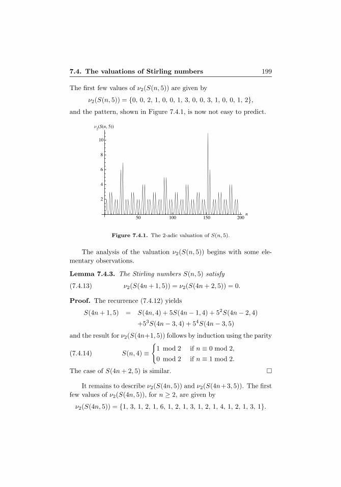
The first few values of ν2(S(n, 5)) are given by
ν2(S(n, 5)) = {0, 0, 2, 1, 0, 0, 1, 3, 0, 0, 3, 1, 0, 0, 1, 2},and the pattern, shown in Figure 7.4.1, is now not easy to predict.
50 100 150 200n
2
4
6
8
10
Figure 7.4.1. The 2-adic valuation of S(n, 5).
The analysis of the valuation ν2(S(n, 5)) begins with some ele-
mentary observations.
Lemma 7.4.3. The Stirling numbers S(n, 5) satisfy
(7.4.13) ν2(S(4n + 1, 5)) = ν2(S(4n + 2, 5)) = 0.
Proof. The recurrence (7.4.12) yields
S(4n + 1, 5) = S(4n, 4) + 5S(4n− 1, 4) + 52S(4n− 2, 4)
+53S(4n− 3, 4) + 54S(4n− 3, 5)
and the result for ν2(S(4n+1, 5)) follows by induction using the parity
(7.4.14) S(n, 4) ≡{
1 mod 2 if n ≡ 0 mod 2,
0 mod 2 if n ≡ 1 mod 2.
The case of S(4n + 2, 5) is similar. �
It remains to describe ν2(S(4n, 5)) and ν2(S(4n+3, 5)). The first
few values of ν2(S(4n, 5)), for n ≥ 2, are given by
ν2(S(4n, 5)) = {1, 3, 1, 2, 1, 6, 1, 2, 1, 3, 1, 2, 1, 4, 1, 2, 1, 3, 1}.
200 7. The Stirling Numbers of the Second Kind
The next step in the analysis of ν2(S(n, 5)) is to show that every
other entry in the values of ν2(S(4n, 5)) is 1.
Lemma 7.4.4. The Stirling numbers S(n, 5) satisfy
ν2(S(8n, 5)) = 1 and ν2(S(8n + 4, 5)) ≥ 2
and also
ν2(S(8n + 3, 5)) = 1 and ν2(S(8n + 7, 5)) ≥ 2.
Proof. The identity
24S(8n, 5) = 58n−1 − 48n + 2 · 38n − 28n+1 + 1
is considered modulo 32. Using 58 ≡ 1 and 57 ≡ 13, it follows that
58n−1 ≡ 13. Also, 48n ≡ 0 and 38n ≡ 1. Therefore
58n−1 − 48n + 2 · 38n − 28n+1 + 1 ≡ 16 mod 32.
This gives 24S(8n, 5) = 32t+16 for some t ∈ N leading to 3S(8n, 5) =
2(2t + 1). Therefore ν2S(8n, 5) = 1.
The valuation of S(8n + 4, 5) comes from the relation
24S(8n + 4, 5) = 58n+3 − 48n+4 + 2 · 38n+4 − 28n+5 + 1
modulo 32. Proceeding as before, it follows that 24S(8n + 4, 5) ≡0 mod 32. Therefore 24S(8n+4, 5) = 32t for some t ∈ N. This yields
ν2(S(8n+ 4, 5)) ≥ 2. The proof of the remaining cases is similar. �
Exercise 7.4.5. Give proofs of Theorems 7.4.1 and 7.4.2 in the style
of the proof of Lemma 7.4.4.
Note 7.4.6. The results described in Lemmas 7.4.3 and 7.4.4 can be
described in terms of a tree similar to the example in Note 1.7.3. The
procedure described here generates the valuation tree associated
to the p-adic valuation of a sequence {xn : n ∈ N}. Each of these
trees has a branching number that depends on the prime p and the
sequence {xn}. The branching number is denoted by b = b(p;xn).
For clarity, in the construction described next, the prime p and the
branching number b will be assumed to be equal to 2.
The construction of the tree begins with a root vertex. This
vertex represents the whole set N and it forms the 0th level of the
tree. Now assume that the kth level has been formed. This level
7.4. The valuations of Stirling numbers 201
represents some of the modular classes modulo 2k. The transition
to the next level is achieved by the following rules: let n0 be the
label of a vertex at the kth level. The label indicates that the vertex
corresponds to the class
an0,k = {n ∈ N : n ≡ n0 mod 2k}.
Then the following question is asked:
Does the valuation {ν2(xn) : n ∈ an0,k} reduce to a single value?
If the answer is yes, the vertex n0 is declared to be a terminal vertex
and the common value of the valuation is attached to n0. If the answer
is no, then the vertex n0 is split into two classes modulo 2k+1, namely,
{n ∈ N : n ≡ n0 mod 2k+1} and {n ∈ N : n ≡ n0 + 2k mod 2k+1}.
The vertices produced by this splitting form the (k + 1)st level.
This process is now applied to the sequence xn = S(n, 5) and the
prime p = 2. The valuation tree starts with a root vertex representing
all N. At this point, the question is whether {ν2(S(n, 5)) : n ∈ N}is independent of n. The values S(5, 5) = 1 and S(7, 5) = 140 =
22 · 5 · 7 show that ν2(S(5, 5)) = 0 and ν2(S(7, 5)) = 2. Therefore the
valuation ν2(S(n, 5)) depends on n and the answer is no. This leads
to a splitting of the root vertex into two vertices: one labeled 0, which
represents the class a0,1 = {n ∈ N : n ≡ 0 mod 2}, and the second
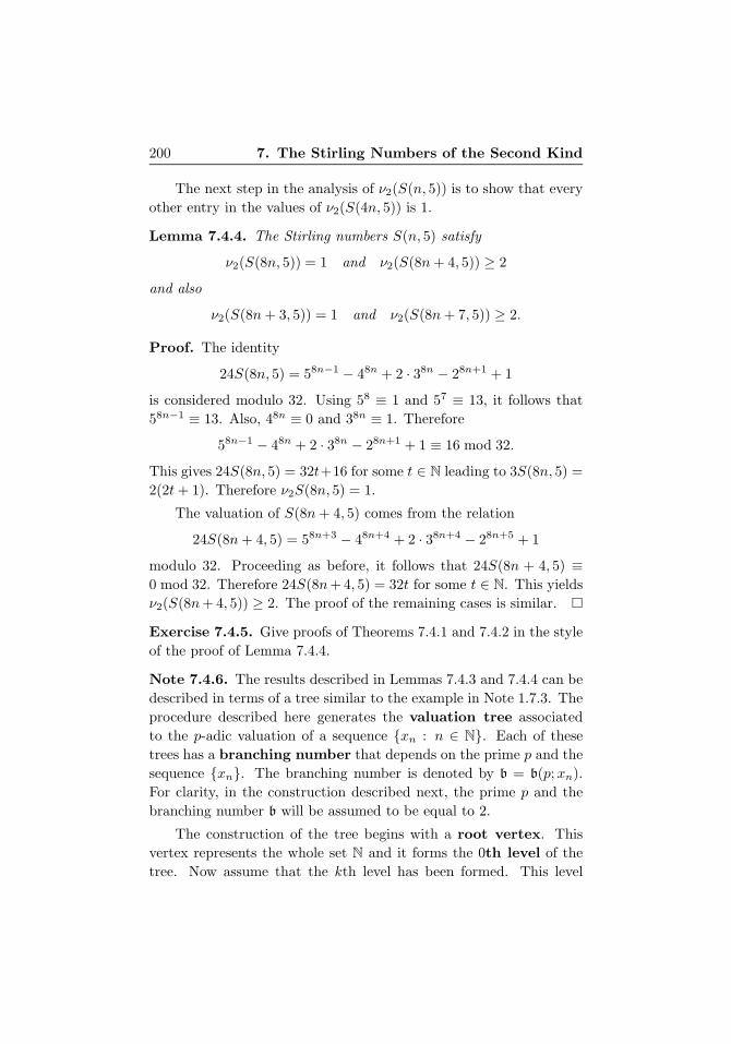
one, labeled 1, representing the class a1,1 = {n ∈ N : n ≡ 1 mod 2}.These two classes form the first level. The reader can check that each
of these two classes do not have a constant 2-adic valuation and the
process continues to the next level.
2n 2n
Figure 7.4.2. The first level of the tree for S(n, 5).
202 7. The Stirling Numbers of the Second Kind
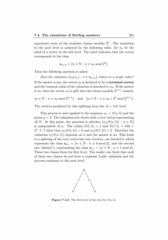
The class a0,1 now splits into
a0,2 = {n ∈ N : n ≡ 0 mod 22} and a2,2 = {n ∈ N : n ≡ 2 mod 22}and a1,1 splits into
a1,2 = {n ∈ N : n ≡ 1 mod 22} and a3,2 = {n ∈ N : n ≡ 3 mod 22}.The construction of the first two levels is depicted in Figure 7.4.3.
2n 2n−1
4n 4n+2 4n+1 4n+3
0 0
Figure 7.4.3. The first two levels of the tree for S(n, 5)
2n 2n
4n 4n 4n 4n
8n 8n 8n 8n
0 0
1 1
+
+ + +
+ +
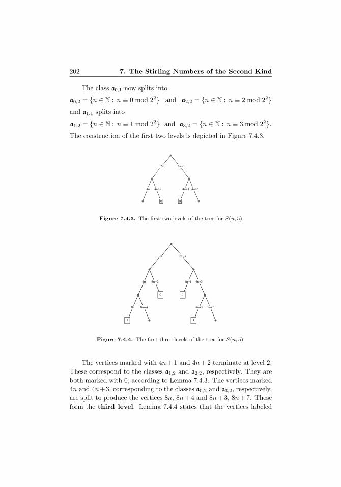
Figure 7.4.4. The first three levels of the tree for S(n, 5).
The vertices marked with 4n+ 1 and 4n+ 2 terminate at level 2.
These correspond to the classes a1,2 and a2,2, respectively. They are
both marked with 0, according to Lemma 7.4.3. The vertices marked
4n and 4n+3, corresponding to the classes a0,2 and a3,2, respectively,
are split to produce the vertices 8n, 8n+4 and 8n+3, 8n+7. These
form the third level. Lemma 7.4.4 states that the vertices labeled
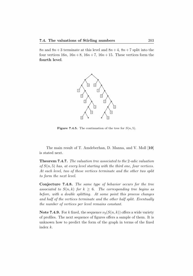
7.4. The valuations of Stirling numbers 203
8n and 8n+3 terminate at this level and 8n+4, 8n+7 split into the
four vertices 16n, 16n+8, 16n+7, 16n+15. These vertices form the
fourth level.
0 0
1 1
2 2
3 3
4 4
5 5
6 6
Figure 7.4.5. The continuation of the tree for S(n, 5).
The main result of T. Amdeberhan, D. Manna, and V. Moll [10]
is stated next.
Theorem 7.4.7. The valuation tree associated to the 2-adic valuation
of S(n, 5) has, at every level starting with the third one, four vertices.
At each level, two of these vertices terminate and the other two split
to form the next level.
Conjecture 7.4.8. The same type of behavior occurs for the tree
associated to S(n, k) for k ≥ 6. The corresponding tree begins as
before, with a double splitting. At some point this process changes
and half of the vertices terminate and the other half split. Eventually
the number of vertices per level remains constant.
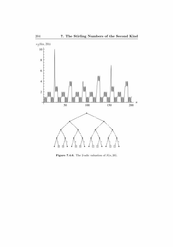
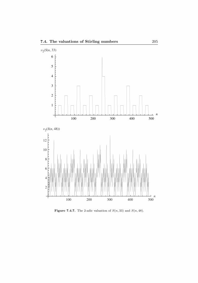
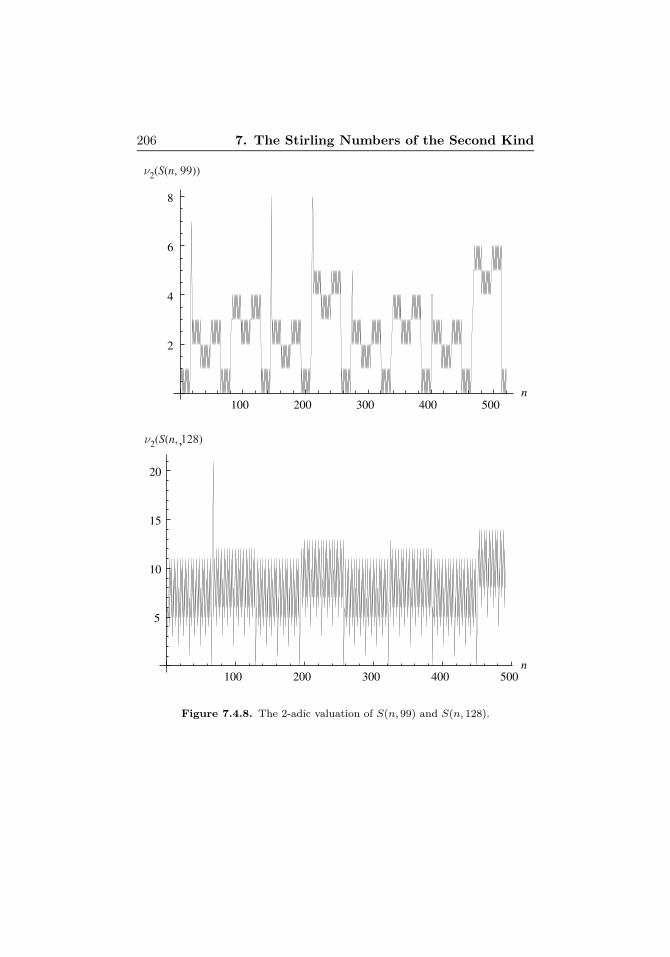
Note 7.4.9. For k fixed, the sequence ν2(S(n, k)) offers a wide variety
of profiles. The next sequence of figures offers a sample of them. It is
unknown how to predict the form of the graph in terms of the fixed
index k.
204 7. The Stirling Numbers of the Second Kind
50 100 150 200n
2
4
6
8
10
0 1
0 2 1 3
0 4 2 6 1 5 3 7
0 8 4 12 2 10 6 14 1 9 5 13 3 11 7 15
0 0 0 0 1 1 1 1
Figure 7.4.6. The 2-adic valuation of S(n, 20).
7.4. The valuations of Stirling numbers 205
100 200 300 400 500n
1
2
3
4
5
6
100 200 300 400 500n
2
4
6
8
10
12
Figure 7.4.7. The 2-adic valuation of S(n, 33) and S(n, 48).
206 7. The Stirling Numbers of the Second Kind
100 200 300 400 500n
2
4
6
8
100 200 300 400 500n
5
10
15
20
Figure 7.4.8. The 2-adic valuation of S(n, 99) and S(n, 128).
7.4. The valuations of Stirling numbers 207
100 200 300 400 500n
2
4
6
8
100 200 300 400 500n
2
4
6
8
10
12
14
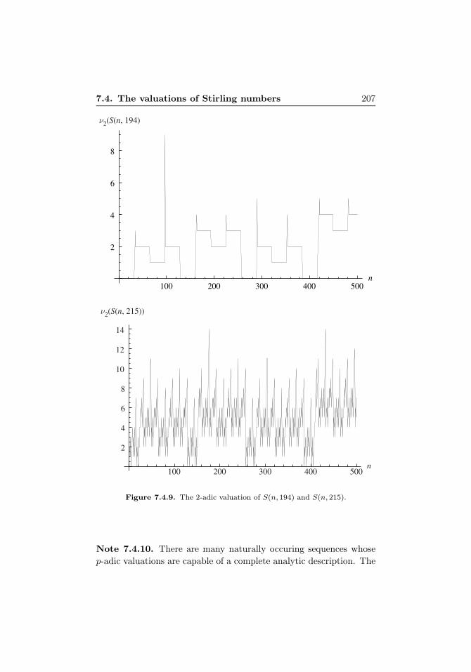
Figure 7.4.9. The 2-adic valuation of S(n, 194) and S(n, 215).
Note 7.4.10. There are many naturally occuring sequences whose
p-adic valuations are capable of a complete analytic description. The
208 7. The Stirling Numbers of the Second Kind
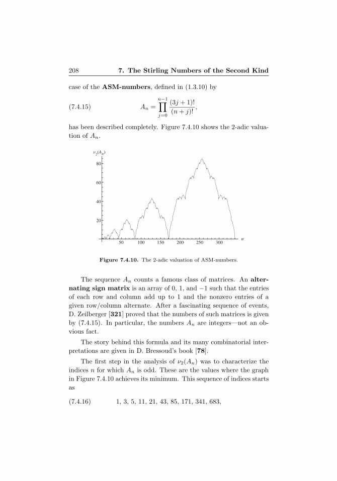
case of the ASM-numbers, defined in (1.3.10) by
(7.4.15) An =
n−1∏j=0
(3j + 1)!
(n + j)!,
has been described completely. Figure 7.4.10 shows the 2-adic valua-
tion of An.
50 100 150 200 250 300n
20
40
60
80
Figure 7.4.10. The 2-adic valuation of ASM-numbers.
The sequence An counts a famous class of matrices. An alter-
nating sign matrix is an array of 0, 1, and −1 such that the entries
of each row and column add up to 1 and the nonzero entries of a
given row/column alternate. After a fascinating sequence of events,
D. Zeilberger [321] proved that the numbers of such matrices is given
by (7.4.15). In particular, the numbers An are integers—not an ob-
vious fact.
The story behind this formula and its many combinatorial inter-
pretations are given in D. Bressoud’s book [78].
The first step in the analysis of ν2(An) was to characterize the
indices n for which An is odd. These are the values where the graph
in Figure 7.4.10 achieves its minimum. This sequence of indices starts
as
(7.4.16) 1, 3, 5, 11, 21, 43, 85, 171, 341, 683,
7.4. The valuations of Stirling numbers 209
and by looking into Sloane’s Encyclopedia of Integer Sequences,
we see that they were recognized as the Jacobsthal numbers, with
label A001045. These numbers satisfy the recurrence
Jn = Jn−1 + 2Jn−2, J0 = 1, J1 = 1.
The many interpretations of these numbers include the number of
ways to tile a 3 × (n − 1) rectangle with squares of size 1 or 2 and
also as the numerators in the reduced fraction
(7.4.17)1
2− 1
4+
1
8− 1
16+
1
32− · · · .
The complete description of the p-adic valuation of ASM-numbers
can be found in the paper by E. Beyerstedt, V. Moll, and X. Sun [53]
as well as in the paper by V. Moll and X. Sun [286].
The main result is an expression for νp(An) similar to the content
of Exercise 2.6.3, where the classical series for the valuation νp(n) is
expressed as a series in which each summand is a periodic function of
period pj .
Theorem 7.4.11. Let n ∈ N and let p ≥ 5 be a prime. Define
Perj,p(n) =
⎧⎪⎪⎪⎪⎪⎪⎨⎪⎪⎪⎪⎪⎪⎩
0 if 0 ≤ n ≤⌊pj+13
⌋,
n−⌊pj+1
3
⌋if⌊pj+13
⌋+ 1 ≤ n ≤ pj−1
2 ,⌊2pj+1
3
⌋− n if pj+1
2 ≤ n ≤⌊2pj+1
3
⌋,
0 if⌊2pj+1
3
⌋+ 1 ≤ n ≤ pj − 1.
Then
νp(An) =
∞∑j=1
Perj,p(n mod pj
).
Each summand in the series is of period pj.
Note 7.4.12. The arithmetical statements about An can be extended
to the sequence
An(q) :=n−1∏j=0
(qj + 1)!
(n + j)!,
for q ∈ N with q ≥ 3. The case of q = 3 corresponds to the ASM-
numbers. An interesting question is to find a combinatorial interpre-
tation of An(q); that is, what do these numbers count?
Chapter 15
Landen Transformations
15.1. Introduction
The transformation of variables plays an important role in the theory
of definite integrals. From the beginning, the reader has been exposed
to some common changes of variables, motivated mainly by the fact
that they work. For example, the basic knowledge of trigonometry
presented in Chapter 12 shows that confronted with a problem of the
type
(15.1.1) I(a, b) =
∫ b
a
dt√1 − t2
,
the change of variables
(15.1.2) t = sinx
leads to a simpler form of the integral.
Naturally, this change of variable, presented in the form
(15.1.3) x = sin−1 t
manifests the new variable of integration as the inverse of a transcen-
dental function.
A different type of map that leaves certain integrals invariant is
defined next.
411
412 15. Landen Transformations
Definition 15.1.1. A Landen transformation for an integral
(15.1.4) I =
∫ x1
x0
f(x;p) dx,
which depends on a set of parameters p, is a map Φ, defined on the
parameters of I, such that
(15.1.5)
∫ x1
x0
f(x;p) dx =
∫ Φ(x1)
Φ(x0)
f(x; Φ(p)) dx.
Example 15.1.2. The classical example of a Landen transformation
is given by
(15.1.6) E(a, b) =
(a + b
2,√ab
),
which preserves the elliptic integral
(15.1.7) G(a, b) =
∫ π/2
0
dx√a2 cos2 x + b2 sin2 x
,
that is,
(15.1.8) G(a, b) = G
(a + b
2,√ab
).
It turns out that the sequence (an, bn) defined inductively by
(15.1.9) (an, bn) = E(an−1, bn−1)
with (a0, b0) = (a, b) has the property that
(15.1.10) limn→∞
an = limn→∞
bn.
This limit is the arithmetic-geometric mean of a and b, denoted
by AGM(a, b). The invariance of the elliptic integral shows that
(15.1.11) G(a, b) =π
2AGM(a, b).
This may be used to compute the elliptic integral G(a, b) by iteration.
This chapter discusses Landen transformations in the case when
the integrand is a rational function. The idea is to produce an appro-
priate change of variables that leaves the rational integral invariant.
The special example
(15.1.12) x = R2(t) =t2 − 1
2t
15.2. An elementary example 413
appearing in Example 8.1.6 leads to the simplest nontrivial class of
Landen transformations.
This chapter contains details of the effect of this map on two
special kinds of integrands. The first one establishes the formula
(15.1.13)
∫ ∞
0
dx
(x4 + 2ax2 + 1)m+1=
π
2
1
[2(1 + a)]m+1/2Pm(a),
where Pm(a) is a polynomial in a.
Warning: The symbol Pm has been used to denote other polynomials
in this text, for instance the Legendre polynomials. In this chapter,
this refers only to the polynomial (15.4.16).
Many properties of its coefficients are presented (not proved) in
this chapter. The second example provides a Landen transformation
for the integral
(15.1.14) U6(a, b; c, d, e) =
∫ ∞
0
cx4 + dx2 + e
x6 + ax4 + bx2 + 1dx,
which leads to an interesting nonlinear transformation.
15.2. An elementary example
The goal of this section is to establish the following result.
Theorem 15.2.1. Let f be a function, with finite integral over R.
Define
(15.2.1) f±(x) = f(x +√x2 + 1) ± f(x−
√x2 + 1)
and
(15.2.2) L(f)(x) = f+(x) +xf−(x)√x2 + 1
.
Then
(15.2.3)
∫ ∞
−∞f(t) dt =
∫ ∞
−∞L(f)(x) dx.
Proof. The map x = R2(t) has two branches separated by the pole
at t = 0. The inverses are given by
(15.2.4) t = x±√x2 + 1.
414 15. Landen Transformations
Each branch maps a half-line onto R. Therefore it is natural to con-
sider integrals over the whole line. The change of variables (15.2.4)
leads to
I =
∫ ∞
−∞f(t) dt
=
∫ 0
−∞f(t) dt +
∫ ∞
0
f(t) dt
=
∫ ∞
−∞f(x−
√x2 + 1)
(1 − x√
x2 + 1
)dx
+
∫ ∞
−∞f(x +
√x2 + 1)
(1 +
x√x2 + 1
)dx.
Now collect terms to obtain the claim. �
Example 15.2.2. Take f(t) = 1/(t2 + 1). Then L(f)(x) = f(x) and
the function f is fixed by L. Now take f(t) = 1/(t2 + 2) to obtain
(15.2.5) L(f)(x) =6
8x2 + 9.
The theorem gives the elementary identity
(15.2.6)
∫ ∞
−∞
dx
x2 + 2=
∫ ∞
−∞
6 dx
8x2 + 9.
Both sides evaluate to π/√
2.
Example 15.2.3. The function f(t) =sin t
tand the value
(15.2.7)
∫ ∞
−∞
sin t
tdt = π
obtained in (12.11.1) lead to the nontrivial integral
(15.2.8)
∫ ∞
−∞
cosx sin√x2 + 1√
x2 + 1dx =
π
2.
The current version of Mathematica (the 8th) is unable to evaluate
this integral.
15.3. The case of rational integrands 415
15.3. The case of rational integrands
In the special case that the integrand f(x) is a rational function,
Theorem 15.2.1 gives an identity among two rational integrals. This
is the content of the next theorem.
Theorem 15.3.1. Assume f(x) is a rational function. Then L(f(x))
is also rational.
Proof. If f(x) is a rational function, then
f(x +√x2 + 1) + f(x−
√x2 + 1)
andf(x +
√x2 + 1) − f(x−
√x2 + 1)√
x2 + 1
are also rational functions. Indeed, let y =√x2 + 1 and assume
f(x) = A(x)/B(x). Then
f(x + y) + f(x− y) =A(x + y)
B(x + y)+
A(x− y)
B(x− y)
=A(x + y)B(x− y) + A(x− y)B(x + y)
B(x + y)B(x− y).
The numerator is a polynomial in x and y, invariant under y �→ −y.
Therefore it is a polynomial in y2 = x2 + 1, thus a polynomial in x.
The same argument applies to the denominator. �
Example 15.3.2. Let
(15.3.1) f(x) =1
4x2 + 12x + 21.
Then
(15.3.2) L(f(x)) =50
336x2 + 408x + 481.
Both integrals may be evaluated in elementary terms to produce the
common value
(15.3.3)
∫ ∞
−∞f(x) dx =
∫ ∞
−∞L(f(x)) dx =
π
4√
3.
416 15. Landen Transformations
Note 15.3.3. A Landen transformation of a rational function has
been defined as a map of the function’s coefficients. For instance,
applying L to the function
(15.3.4) f(x) =1
ax2 + bx + c
yields
(15.3.5) L(f(x)) =1
a1x2 + b1x + c1
with
(15.3.6) a1 =2 c a
c + a, b1 =
b(c− a)
c + a, c1 =
(c + a)2 − b2
2(c + a).
Exercise 15.3.4. Check that the discriminant of the denominator is
preserved, that is, b2 − 4ac = b21 − 4a1c1.
Note 15.3.5. Define
(15.3.7) Φ2(a, b, c) = (a1, b1, c1)
with (a1, b1, c1) given in (15.3.6). Iteration of Φ2 gives a sequence
(an, bn, cn) that preserves the original integral
(15.3.8)
∫ ∞
−∞
dx
anx2 + bnx + cn=
∫ ∞
−∞
dx
ax2 + bx + c.
Exercise 15.3.6. Prove that (an, bn, cn) converges to (L, 0, L), for
some L ∈ R, under the assumption b2 − 4ac < 0.
Passing to the limit in (15.3.8) shows that
(15.3.9)
∫ ∞
−∞
dx
ax2 + bx + c=
π
L.
In the case a > 0, the limiting value
(15.3.10) L =1
2
√4ac− b2
is obtained from (15.3.9) by computing the integral. The case of a < 0
is similar.
The map Φ2 is the rational analog of the classical arithmetic-
geometric mean presented at the beginning of this chapter. A
discussion of this case is presented in Section 15.6.
15.4. The evaluation of a quartic integral 417
Exercise 15.3.7. It is possible for a single integral to admit a variety
of Landen transformations. For instance the quadratic integral
(15.3.11)
∫ ∞
−∞
dx
ax2 + bx + c
is also invariant under the change of parameters
an+1 = an
[(an+3cn)
2−3b2n(3an+cn)(an+3cn)−b2n
],(15.3.12)
bn+1 = bn
[3(an−cn)
2−b2n(3an+cn)(an+3cn)−b2n
],
cn+1 = cn
[(3an+cn)
2−3b2n(3an+cn)(an+3cn)−b2n
],
with a0 = a, b0 = b, and c0 = c. This is described in complete
detail in the paper by D. Manna and V. Moll [208]. Follow the steps
given there to show that iteration of this converges to the stated limit
(L, 0, L).
15.4. The evaluation of a quartic integral
This section contains an application of the transformation L intro-
duced in Theorem 15.2.1 to the evaluation of the definite integral
(15.4.1) N0,4(a;m) =
∫ ∞
0
dx
(x4 + 2ax2 + 1)m+1.
The first theorem describes the effect of L on the integrand.
Theorem 15.4.1. For m ∈ N, let
(15.4.2) Q(x) =1
(x4 + 2ax2 + 1)m+1.
Then
(15.4.3) Q1(y) := L(Q(x)) =Tm(2y)
2m(1 + a + 2y2)m+1,
where
(15.4.4) Tm(y) =
m∑k=0
(m + k
m− k
)y2k.
418 15. Landen Transformations
Proof. Introduce the variable φ = y+√y2 + 1. Then y−
√y2 + 1 =
−φ−1 and 2y = φ− φ−1. Moreover,
Q1(y) =[Q(φ) + Q(φ−1)
]+
φ2 − 1
φ2 + 1
(Q(φ) −Q(φ−1)
)=
2
φ2 + 1
[φ2Q(φ) + Q(φ−1)
]:= Sm(φ).
Then (15.4.3) is equivalent to
(15.4.5) 2m(1 + a + 1
2 (φ− φ−1)2)m+1
Sm(φ) = Tm(φ− φ−1).
A direct (but lengthy) simplification of the left-hand side of (15.4.5)
shows that this identity is equivalent to proving
(15.4.6)φ2m+1 + φ−(2m+1)
φ + φ−1= Tm(φ− φ−1).
Observe that the parameter a has disappeared.
First proof. One simply checks that both sides of (15.4.6) satisfy
the second-order recurrence
(15.4.7) cm+2 − (φ2 + φ−2)cm+1 + cm = 0
and that the values for m = 0 and m = 1 match. This is straight-
forward for the expression on the left-hand side, while the WZ-method
settles the right-hand side. �
Second proof. In the textbook by R. Graham, D. Knuth, and
O. Patashnik [145], one finds the generating function
(15.4.8) Bt(z) =∑k≥0
(tk)k−1zk
k!,
where (a)k = a(a+1) · · · (a+ k− 1) is the Pochhammer symbol. The
special values
(15.4.9) B−1(z) =1 +
√1 + 4z
2and B2(z) =
1 −√
1 − 4z
2z
are combined to produce the identity
1√1 + 4z
(B−1(z)
n+1 − (−z)n+1B2(−z)n+1)
=n∑
k=0
(n− k
k
)zk.
15.4. The evaluation of a quartic integral 419
Replace n by 2m and z by (4y2)−1 to produce
1
2√
1 + y2 (2y)2m(φ2m+1 + φ−(2m+1)) =
m∑k=0
(2m− k
k
)zk.
The sum on the right-hand side is simplified by the identity
Tm(y) =m∑
k=0
(m + k
m− k
)y2k = y2m
m∑k=0
(2m− k
k
)y−2k.
Thus,
Tm(φ− φ−1) = Tm(2y) = (2y)2mm∑
k=0
(2m− k
k
)zk,
and it follows that
Tm(φ− φ−1) =1
2√
1 + y2(φ2m+1 + φ−(2m+1)),
and the result is obtained from φ + φ−1 = 2√y2 + 1.
Evaluation of the integral N0,4(a;m). The identity in Theorem
15.2.1 shows that
(15.4.10)
∫ ∞
0
Q(x) dx =
∫ ∞
0
Q1(y) dy,
and this last integral can be evaluated in elementary form. Indeed,∫ ∞
0
Q1(y) dy =
∫ ∞
0
Tm(2y) dy
2m(1 + 2y2)m+1
=1
2m
m∑k=0
(m + k
m− k
)∫ ∞
0
(2y)2k dy
(1 + a + 2y2)m+1.
The change of variables y = t√
1 + a/√
2 gives∫ ∞
0
Q1(y) dy =1
[2(1 + a)]m+1/2
m∑k=0
(m + k
m− k
)2k(1+a)k
∫ ∞
0
t2k dt
(1 + t2)m+1.
Exercise 15.4.2. Prove the Wallis-type identity
(15.4.11)
∫ ∞
0
t2k dt
(1 + t2)m+1=
π
22m+1
(2k
k
)(2m− 2k
m− k
)(m
k
)−1
.
420 15. Landen Transformations
The previous exercise now produces∫ ∞
0
Q1(y) dy =π
22m+1
1
[2(1 + a)]m+1/2
×m∑
k=0
(m + k
m− k
)2k(
2k
k
)(2m− 2k
m− k
)(m
k
)−1
(1 + a)k.
This can be simplified further using
(15.4.12)
(m + k
m− k
)(2k
k
)=
(m + k
m
)(m
k
), 0 ≤ k ≤ m,
and (15.4.10) to produce∫ ∞
0
Q(y) dy =π
22m+1
1
[2(1 + a)]m+1/2
m∑k=0
2k(m + k
m
)(2m− 2k
m− k
)(1+a)k.
Theorem 15.4.3. The integral N0,4(a;m), defined in (15.4.1), is
given by
(15.4.13) N0,4(a;m) =π
2
1
[2(1 + a)]m+1/2
m∑j=0
dj,maj ,
where
(15.4.14) dj,m = 2−2mm∑
k=j
2k(
2m− 2k
m− k
)(m + k
m
)(k
j
).
Note 15.4.4. The literature contains a variety of proofs of the for-
mula given in Theorem 15.4.3. This is written here as
(15.4.15)
N0,4(a;m) =
∫ ∞
0
dx
(x4 + 2ax2 + 1)m+1=
π
2
Pm(a)
[2(a + 1)]m+1/2
where
(15.4.16) Pm(a) =
m∑j=0
dj,maj .
This note discusses some of these proofs and highlights the remarkable
properties of the coefficients dj,m.
The first proof. This proof is due to George Boros, a former stu-
dent of the author. The idea is remarkably simple but has profound

15.4. The evaluation of a quartic integral 421
consequences. The change of variables x = tan θ yields
N0,4(a;m) =
∫ π/2
0
(cos4 θ
sin4 θ + 2a sin2 θ cos2 θ + cos4 θ
)m+1
× dθ
cos2 θ.
Observe that the denominator of the integrand is a polynomial in
cos 2θ. In terms of the double-angle u = 2θ, the original integral
becomes
N0,4(a;m) = 2−(m+1)
∫ π
0
((1 + cosu)2
(1 + a) + (1 − a) cos2 u
)m+1
× du
1 + cosu.
Expanding the binomial (1 + cosu)2m+1, symmetry implies that∫ π
0
(cosu)j du
[(1 + a) + (1 − a) cos2 u]m+1= 0,
for j odd. The remanining integrals, those with j even, can be eval-
uated by using the double-angle trick one more time. This leads to
N0,4(a;m) =m∑j=0
2−j
(2m + 1
2j
)∫ π
0
(1 + cos v)j dv
[(3 + a) + (1 − a) cos v]m+1,
where v = 2u and the symmetry of cosine about v = π has been used
to reduce the integrals from [0, 2π] to [0, π]. The familiar change of
variables z = tan(v/2) produces the form (15.4.15). The expression
obtained for the coefficients dj,m is not very pretty:
dj,m =
j∑r=0
m−j∑s=0
m∑k=j+s
(−1)k−j−s
23k
(2k
k
)(2m + 1
2s + 2r
)(m− s− r
m− k
)
×(s + r
r
)(k − s− r
j − r
).
A detour into the world of Ramanujan. The search for a simpler
expression for the coefficients dj,m began with the observation that
they appear to be positive. Indeed, a symbolic calculation shows that
for m = 5, these are
{dj,5 : 0 ≤ j ≤ 5} =
{4389
256,
8589
128,
7161
64,
777
8,
693
16,
63
8
}.
422 15. Landen Transformations
The second proof of (15.4.15) begins with the value of the elementary
integral
(15.4.17)
∫ ∞
0
dx
bx4 + 2ax2 + 1=
π
2√
2
1√a +
√b
and the functions h(c) =√a +
√1 + c and
g(c) =
∫ ∞
0
dx
x4 + 2ax2 + 1 + c.
Then (15.4.17) gives g′(c) = π√
2h′(c). In particular,
h′(0) =1
π√
2N0,4(a; 0).
Further differentiation gives the higher-order derivatives of h in terms
of the integrals N0,4. This is expressed as
Theorem 15.4.5. The Taylor expansion of h(c) =√a +
√1 + c is
given by√a +
√1 + c =
√a + 1 +
1
π√
2
∞∑k=1
(−1)k−1
kN0,4(a; k − 1)ck.
The evaluation of the integrals N0,4(a;m) is now finished by using
the Ramanujan master theorem stated below.
Theorem 15.4.6. Suppose F has a Taylor expansion around c = 0
of the form
F (c) =
∞∑k=0
(−1)k
k!ϕ(k) ck.
Then, the moments of F , defined by
Mn =
∫ ∞
0
cn−1F (c) dc,
can be computed via Mn = Γ(n)ϕ(−n).
B. Berndt [49], in the first volume of Ramanujan’s Notebooks,
provides a proof of the exact hypothesis for the validity of this the-
orem. Applications to the evaluation of a large variety of definite
integrals are given in the paper by T. Amdeberhan, O. Espinosa,
I. Gonzalez, M. Harrison, V. Moll, and A. Straub [8]. It turns out
15.4. The evaluation of a quartic integral 423
that, in the case considered here, the moments can be evaluated ex-
plicitly, leading to the proof. Details can be found in the paper by
G. Boros and V. Moll [64].
A nice short proof. The following argument was communicated to
the author by M. Hirschhorn [171]. Start with
I =
∫ ∞
0
dx
x4 + 2ax2 + 1.
Make the substitution x �→ 1/x and add the two forms of the integral
I to obtain
2I =
∫ ∞
0
(x2 + 1) dx
x4 + 2ax2 + 1.
The second substitution y = x− 1/x gives
2I =
∫ ∞
−∞
dy
y2 + 2a + 2=
π√2a + 2
.
Now, for an appropriate value of c (to guarantee convergence),∫ ∞
0
dx
x4 + 2ax2 + c2=
π
2√
2√a + c
.
Differentiation with respect to c leads to the identity∫ ∞
0
dx
(x4 + 2ax2 + c2)m+1=
π
23m+3/2 c2m+1 (a + c)m+1/2
×m∑
k=0
2m−k
(2k
k
)(2m− k
m
)ck(a + c)m−k.
The result now follows by taking c = 1.
Proofs in other styles. There are several other proofs of Theorem
15.4.3 in the literature. The paper by G. Boros and V. Moll [62]
produced a proof based on elementary properties of the hypergeo-
metric function plus an entry from the table by I. S. Gradshteyn and
I. M. Ryzhik [144]. A new proof based on a method for the evaluation
of integrals coming from Feynman diagrams appears in the paper by
T. Amdeberhan, V. Moll, and C. Vignat [15]. An automatic proof
has appeared in the work of C. Koutschan and V. Levandovskyy [187]
and one more based on the study of statistical densities can be found
in the work by C. Berg and C. Vignat [48]. Finally, a nice evaluation
combining classical and automatic methods appears in the paper by
424 15. Landen Transformations
M. Apagodu [23]. The reader is encouraged to produce his/her
own.
The coefficients dj,m. These numbers have remarkable properties.
A related family of polynomials . Start with
Pm(a) =2
π[2(a + 1)]m+
12
∫ ∞
0
dx
(x4 + 2ax2 + 1)m+1,
and compute dj,m as coming from the Taylor expansion at a = 0 of
the right-hand side. This yields
(15.4.18)
dj,m =1
j!m!2m+j
(αj(m)
m∏k=1
(4k − 1) − βj(m)
m∏k=1
(4k + 1)
),
where αj and βj are polynomials in m of degrees j and j − 1, respec-
tively. The explicit expressions
αj(m) =
�j/2�∑t=0
(j
2t
) m+t∏ν=m+1
(4ν − 1)
m∏ν=m−j+2t+1
(2ν + 1)
t−1∏ν=1
(4ν + 1)
and
βj(m) =
�(j+1)/2�∑t=1
(j
2t− 1
) m+t−1∏ν=m+1
(4ν+1)
m∏ν=m−j+2t
(2ν+1)
t−1∏ν=1
(4ν−1)
are given in the paper by G. Boros, V. Moll, and J. Shallit [67].
Trying to obtain more information about the polynomials αj and
βj directly proved difficult. One uninspired day, the author decided
to compute their roots numerically. It was a pleasant surprise to
discover the following property.
Theorem 15.4.7. For all j ≥ 1, all the roots of αj(m) = 0 lie on
the line Rem = − 12 . Similarly, the roots of βj(m) = 0 for j ≥ 2 lie
on the same vertical line.
The proof of this theorem, due to J. Little [201], starts by writing
(15.4.19) Aj(s) := αj((s− 1)/2) and Bj(s) := βj((s− 1)/2)
15.4. The evaluation of a quartic integral 425
and proving that Aj is equal to j! times the coefficient of uj in
f(s, u)g(s, u), where f(s, u) = (1 + 2u)s/2 and g(s, u) is the hyperge-
ometric series
(15.4.20) g(s, u) = 2F1
(s
2+
1
4,1
4;1
2; 4u2
).
A similar expression is obtained for Bj(s). From here it follows that
Aj and Bj each satisfy the three-term recurrence
(15.4.21) xj+1(s) = 2sxj(s) − (s2 − (2j − 1)2)xj−1(s).
Little then establishes a version of Sturm’s theorem about interlacing
zeros to prove the final result.
The location of the zeros of αj(m) now suggests studying the
behavior of this family as j → ∞. In the best of all worlds, one will
obtain an analytic function of m with all the zeros on a vertical line.
Perhaps some number theory will enter and . . . one never knows.
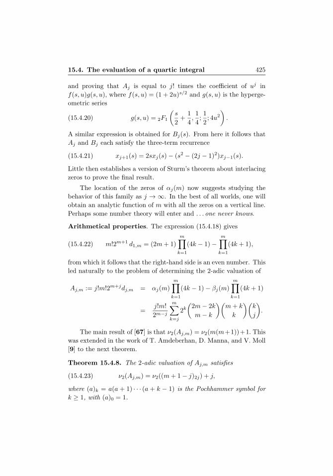
Arithmetical properties. The expression (15.4.18) gives
(15.4.22) m!2m+1 d1,m = (2m + 1)
m∏k=1
(4k − 1) −m∏
k=1
(4k + 1),
from which it follows that the right-hand side is an even number. This
led naturally to the problem of determining the 2-adic valuation of
Aj,m := j!m!2m+jdj,m = αj(m)
m∏k=1
(4k − 1) − βj(m)
m∏k=1
(4k + 1)
=j!m!
2m−j
m∑k=j
2k(
2m− 2k
m− k
)(m + k
k
)(k
j
).
The main result of [67] is that ν2(Aj,m) = ν2(m(m+1))+1. This
was extended in the work of T. Amdeberhan, D. Manna, and V. Moll
[9] to the next theorem.
Theorem 15.4.8. The 2-adic valuation of Aj,m satisfies
(15.4.23) ν2(Aj,m) = ν2((m + 1 − j)2j) + j,
where (a)k = a(a + 1) · · · (a + k − 1) is the Pochhammer symbol for
k ≥ 1, with (a)0 = 1.
426 15. Landen Transformations
The proof is an elementary application of the WZ-method. Define
the numbers
Bj,m :=Aj,m
2j(m + 1 − j)2j,
and use the WZ-method to obtain the recurrence
Bj−1,m = (2m+1)Bj,m− (m− j)(m+ j+1)Bj+1,m, 1 ≤ j ≤ m−1.
Since the initial values Bm,m = 1 and Bm−1,m = 2m + 1 are odd, it
follows inductively that Bj,m is an odd integer. The reader will also
find in [9] a WZ-free proof of the theorem.
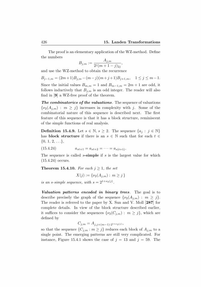
The combinatorics of the valuations . The sequence of valuations
{ν2(Aj,m) : m ≥ j} increases in complexity with j. Some of the
combinatorial nature of this sequence is described next. The first
feature of this sequence is that it has a block structure, reminiscent
of the simple functions of real analysis.
Definition 15.4.9. Let s ∈ N, s ≥ 2. The sequence {aj : j ∈ N}has block structure if there is an s ∈ N such that for each t ∈{0, 1, 2, . . .},(15.4.24) ast+1 = ast+2 = · · · = as(t+1).
The sequence is called s-simple if s is the largest value for which
(15.4.24) occurs.
Theorem 15.4.10. For each j ≥ 1, the set
X(j) := {ν2(Aj,m) : m ≥ j }is an s-simple sequence, with s = 21+ν2(j).
Valuation patterns encoded in binary trees . The goal is to
describe precisely the graph of the sequence {ν2(Aj,m) : m ≥ j}.The reader is referred to the paper by X. Sun and V. Moll [287] for
complete details. In view of the block structure described earlier,
it suffices to consider the sequences {ν2(Cj,m) : m ≥ j}, which are
defined by
Cj,m = Aj,j+(m−1)·21+ν2(j) ,
so that the sequence {Cj,m : m ≥ j} reduces each block of Aj,m to a
single point. The emerging patterns are still very complicated. For
instance, Figure 15.4.1 shows the case of j = 13 and j = 59. The
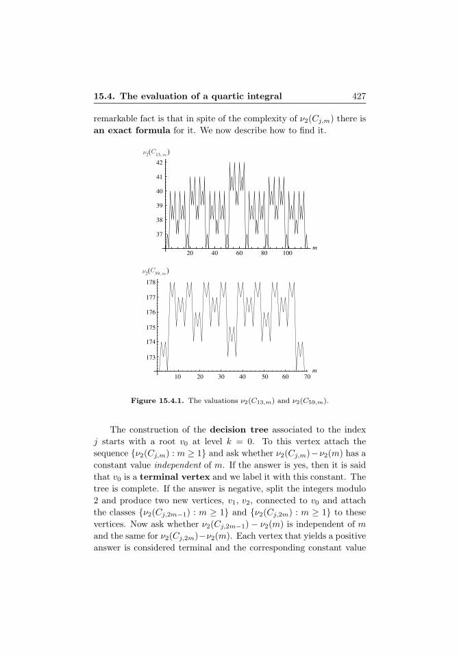
15.4. The evaluation of a quartic integral 427
remarkable fact is that in spite of the complexity of ν2(Cj,m) there is
an exact formula for it. We now describe how to find it.
20 40 60 80 100m
37
38
39
40
41
42
ν2(C13, m)
10 20 30 40 50 60 70m
173
174
175
176
177
178
ν2(C59, m)
Figure 15.4.1. The valuations ν2(C13,m) and ν2(C59,m).
The construction of the decision tree associated to the index
j starts with a root v0 at level k = 0. To this vertex attach the
sequence {ν2(Cj,m) : m ≥ 1} and ask whether ν2(Cj,m)−ν2(m) has a
constant value independent of m. If the answer is yes, then it is said
that v0 is a terminal vertex and we label it with this constant. The
tree is complete. If the answer is negative, split the integers modulo
2 and produce two new vertices, v1, v2, connected to v0 and attach
the classes {ν2(Cj,2m−1) : m ≥ 1} and {ν2(Cj,2m) : m ≥ 1} to these
vertices. Now ask whether ν2(Cj,2m−1) − ν2(m) is independent of m
and the same for ν2(Cj,2m)−ν2(m). Each vertex that yields a positive
answer is considered terminal and the corresponding constant value
428 15. Landen Transformations
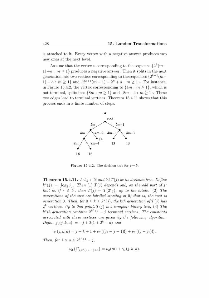
is attached to it. Every vertex with a negative answer produces two
new ones at the next level.
Assume that the vertex v corresponding to the sequence {2k(m−1)+a : m ≥ 1} produces a negative answer. Then it splits in the next
generation into two vertices corresponding to the sequences {2k+1(m−1) + a : m ≥ 1} and {2k+1(m− 1) + 2k + a : m ≥ 1}. For instance,
in Figure 15.4.2, the vertex corresponding to {4m : m ≥ 1}, which is
not terminal, splits into {8m : m ≥ 1} and {8m− 4 : m ≥ 1}. These
two edges lead to terminal vertices. Theorem 15.4.11 shows that this
process ends in a finite number of steps.
root
2m
4m
8m 1314
13
16 16
Figure 15.4.2. The decision tree for j = 5.
Theorem 15.4.11. Let j ∈ N and let T (j) be its decision tree. Define
k∗(j) := �log2 j�. Then (1) T (j) depends only on the odd part of j;
that is, if r ∈ N, then T (j) = T (2rj), up to the labels. (2) The
generations of the tree are labelled starting at 0; that is, the root is
generation 0. Then, for 0 ≤ k ≤ k∗(j), the kth generation of T (j) has
2k vertices. Up to that point, T (j) is a complete binary tree. (3) The
k∗th generation contains 2k∗+1 − j terminal vertices. The constants
associated with these vertices are given by the following algorithm.
Define j1(j, k, a) := −j + 2(1 + 2k − a) and
γ1(j, k, a) = j + k + 1 + ν2 ((j1 + j − 1)!) + ν2 ((j − j1)!) .
Then, for 1 ≤ a ≤ 2k∗+1 − j,
ν2(Cj,2k(m−1)+a
)= ν2(m) + γ1(j, k, a).
15.4. The evaluation of a quartic integral 429
Thus, the vertices at the k∗th generation have constants given by
γ1(j, k, a). (4) The remaining terminal vertices of the tree T (j) ap-
pear in the next generation. There are 2(j − 2k∗(j)) of them. The
constants attached to these vertices are defined as follows: let
j2(j, k, a) := −j+2(1+2k+1−a) and j3(j, k, a) := j2(j, k, a+2k).
Define
γ2(j, k, a) := j + k + 2 + ν2 ((j2 + j − 1)!) + ν2 ((j − j2)!)
and
γ3(j, k, a) := j + k + 2 + ν2 ((j3 + j − 1)!) + ν2 ((j − j3)!) .
Then, for 2k∗(j)+1 − j + 1 ≤ a ≤ 2k
∗(j),
ν2(Cj,2k∗(j)+1(m−1)+a
)= ν2(m) + γ2(j, k
∗(j), a)
and
ν2(Cj,2k∗(j)+1(m−1)+a+2k∗(j)
)= ν2(m) + γ3(j, k
∗(j), a)
give the constants attached to these remaining terminal vertices.
The theorem is now employed to produce an analytic formula
for ν2(C3,m). The value k∗(3) = 1 shows that the first level contains
21+1−3 = 1 terminal vertex. This corresponds to the sequence 2m−1
and has constant value 7. Thus,
(15.4.25) ν2 (C3,2m−1) = 7.
The next level has 2(3− 21) = 2 terminal vertices. These correspond
to the sequences 4m and 4m − 2, with constant value 9 for both of
them. This tree produces
(15.4.26) ν2 (C3,m) =
⎧⎪⎪⎨⎪⎪⎩
7 + ν2(m+12
)if m ≡ 1 mod 2,
9 + ν2(m4
)if m ≡ 0 mod 4,
9 + ν2(m+24
)if m ≡ 2 mod 4.
430 15. Landen Transformations
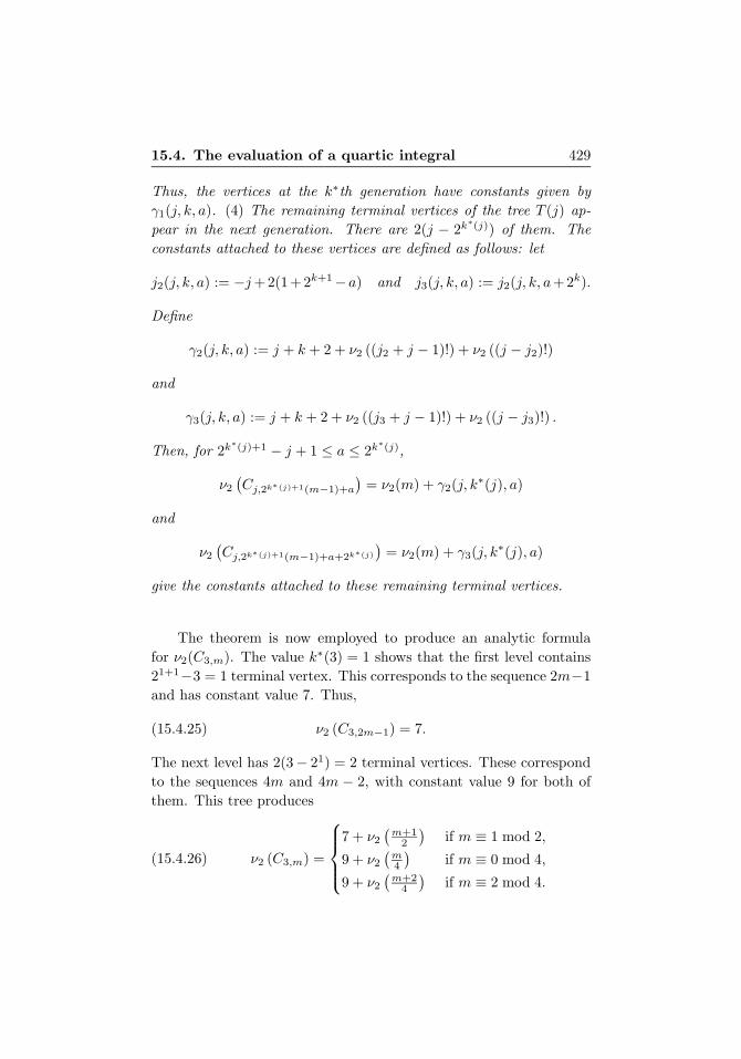
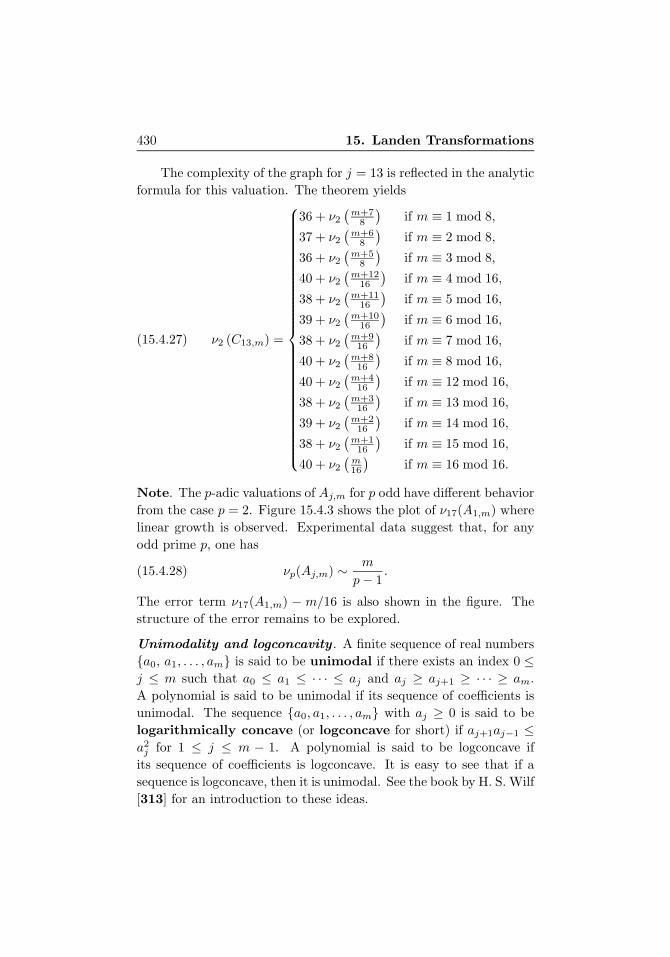
The complexity of the graph for j = 13 is reflected in the analytic
formula for this valuation. The theorem yields
(15.4.27) ν2 (C13,m) =
⎧⎪⎪⎪⎪⎪⎪⎪⎪⎪⎪⎪⎪⎪⎪⎪⎪⎪⎪⎪⎪⎪⎪⎪⎪⎪⎪⎪⎨⎪⎪⎪⎪⎪⎪⎪⎪⎪⎪⎪⎪⎪⎪⎪⎪⎪⎪⎪⎪⎪⎪⎪⎪⎪⎪⎪⎩
36 + ν2(m+78
)if m ≡ 1 mod 8,
37 + ν2(m+68
)if m ≡ 2 mod 8,
36 + ν2(m+58
)if m ≡ 3 mod 8,
40 + ν2(m+1216
)if m ≡ 4 mod 16,
38 + ν2(m+1116
)if m ≡ 5 mod 16,
39 + ν2(m+1016
)if m ≡ 6 mod 16,
38 + ν2(m+916
)if m ≡ 7 mod 16,
40 + ν2(m+816
)if m ≡ 8 mod 16,
40 + ν2(m+416
)if m ≡ 12 mod 16,
38 + ν2(m+316
)if m ≡ 13 mod 16,
39 + ν2(m+216
)if m ≡ 14 mod 16,
38 + ν2(m+116
)if m ≡ 15 mod 16,
40 + ν2(m16
)if m ≡ 16 mod 16.
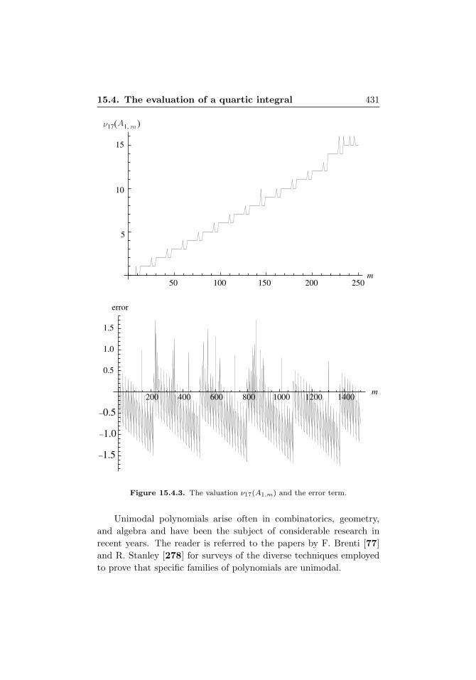
Note. The p-adic valuations of Aj,m for p odd have different behavior
from the case p = 2. Figure 15.4.3 shows the plot of ν17(A1,m) where
linear growth is observed. Experimental data suggest that, for any
odd prime p, one has
(15.4.28) νp(Aj,m) ∼ m
p− 1.
The error term ν17(A1,m) − m/16 is also shown in the figure. The
structure of the error remains to be explored.
Unimodality and logconcavity . A finite sequence of real numbers
{a0, a1, . . . , am} is said to be unimodal if there exists an index 0 ≤j ≤ m such that a0 ≤ a1 ≤ · · · ≤ aj and aj ≥ aj+1 ≥ · · · ≥ am.
A polynomial is said to be unimodal if its sequence of coefficients is
unimodal. The sequence {a0, a1, . . . , am} with aj ≥ 0 is said to be
logarithmically concave (or logconcave for short) if aj+1aj−1 ≤a2j for 1 ≤ j ≤ m − 1. A polynomial is said to be logconcave if
its sequence of coefficients is logconcave. It is easy to see that if a
sequence is logconcave, then it is unimodal. See the book by H. S. Wilf
[313] for an introduction to these ideas.
15.4. The evaluation of a quartic integral 431
50 100 150 200 250m
5
10
15
ν17(A1, m)
200 400 600 800 1000 1200 1400m
0.5
1.0
1.5
error
Figure 15.4.3. The valuation ν17(A1,m) and the error term.
Unimodal polynomials arise often in combinatorics, geometry,
and algebra and have been the subject of considerable research in
recent years. The reader is referred to the papers by F. Brenti [77]
and R. Stanley [278] for surveys of the diverse techniques employed
to prove that specific families of polynomials are unimodal.
432 15. Landen Transformations
For m ∈ N, the sequence {dj,m : 0 ≤ j ≤ m} is unimodal. This is
a consequence of the following criterion established in the paper by
G. Boros and V. Moll [61].
Theorem 15.4.12. Let ak be a nondecreasing sequence of positive
numbers and let A(x) =∑m
k=0 akxk. Then A(x + 1) is unimodal.
This theorem was applied to the polynomial
(15.4.29) A(x) := 2−2mm∑
k=0
2k(
2m− 2k
m− k
)(m + k
m
)xk
that satisfies Pm(x) = A(x + 1). The criterion was extended in a
project at SIMU (Summer Institute in Mathematics for Undergrad-
uates), an REU program in Puerto Rico. The result was the paper
by J. Alvarez, M. Amadis, G. Boros, D. Karp, V. Moll, and L. Ros-
ales [7] to include the shifts A(x + j) and the paper by Yi Yang and
Yeong-Nan Yeh [304] for arbitrary shifts. The original proof of the
unimodality of Pm(a) can be found in the paper by G. Boros and
V. Moll [63].
The author conjectured in [221] the logconcavity of {dj,m : 0 ≤j ≤ m}. This turned out to be a more difficult question. Some of our
failed attempts are described next.
(1) A result of F. Brenti [77] states that if A(x) is logconcave,
then so is A(x + 1). Unfortunately this does not apply in this case
since (15.4.29) is not logconcave. Indeed,
24m−2k(a2k − ak−1ak+1
)=
(2m
m− k
)2(m + k
m
)2
×(
1 − k(m− k)(2m− 2k + 1)(m + k + 1)
(k + 1)(m + k)(2m− 2k − 1)(m− k + 1)
)and this last factor could be negative—for example, for m = 5 and
j = 4. The number of negative terms in this sequence is small, so
perhaps there is a way out of this.
(2) The coefficients dj,m satisfy many recurrences. For example,
dj+1,m =2m + 1
j + 1dj,m − (m + j)(m + 1 − j)
j(j + 1)dj−1,m.
15.4. The evaluation of a quartic integral 433
This can be found by a direct application of the WZ-method. There-
fore, dj,m is logconcave provided
j(2m + 1)dj−1,mdj,m ≤ (m + j)(m + 1 − j)d2j−1,m + j(j + 1)d2j,m.
The author conjectured that the smallest value of the expression
(m + j)(m + 1 − j)d2j−1,m + j(j + 1)d2j,m − j(2m + 1)dj−1,mdj,m
is 22mm(m + 1)(2mm
)2and it occurs at j = m. This has been es-
tablished by W. Y. C. Chen and E. X. W. Yia [99]. It implies the
logconcavity of {dj,m : 0 ≤ j ≤ m}.Actually, the author has conjectured that the dj,m satisfy a
stronger version of logconcavity. Given a sequence {aj} of positive
numbers, define a map
L ({aj}) := {bj}
by bj := a2j − aj−1aj+1. Thus {aj} is logconcave if {bj} has positive
coefficients. The nonnegative sequence {aj} is called infinitely log-
concave if any number of applications of L produces a nonnegative
sequence.
Conjecture 15.4.13. For each fixed m ∈ N, the sequence {dj,m :
0 ≤ j ≤ m} is infinitely logconcave.
The logconcavity of {dj,m : 0 ≤ j ≤ m} has recently been estab-
lished by M. Kauers and P. Paule [180] as an applications of their
work on establishing inequalities by automatic means. The starting
point is the triple sum expression for dj,m written as
dj,m =∑j,s,k
(−1)k+j−l
23(k+s)
(2m + 1
2s
)(m− s
k
)(2(k + s)
k + s
)(s
j
)(k
l − j
).
Using the RISC (Research Institute for Symbolic Computation) pack-
age Multisim developed by K. Wegschaider [308], Kauers and Paule
derived the recurrence
2(m + 1)dj,m+1 = 2(j + m)dj−1,m + (2j + 4m + 3)dj,m.
434 15. Landen Transformations
The positivity of dj,m follows directly from this. To establish the
logconcavity of dj,m, the new recurrence
4j(j + 1)dj+1,m = −2(2j − 4m− 3)(j + m + 1)dj,m
+ 4(j −m− 1)(m + 1)dj,m+1
is derived automatically and the logconcavity of dj,m is reduced toestablishing the inequality
d2j,m ≥4(m+ 1)
(4(j −m− 1)(m+ 1)− (2j2 − 4m2 − 7m− 3)dj,m+1dj,m
)16m3 + 16jm2 + 40m2 + 28jm+ 33m+ 9j + 9
.
This is now accomplished in automatic fashion.
The 2-logconcavity of {dj,m : 0 ≤ j ≤ m} is not achievable by
these methods. At the end of [180], M. Kauers and P. Paule state
that “...we have little hope that a proof of 2-logconcavity could be
completed along these lines, not to mention that a human reader
would have a hard time digesting it.” Actually, 2-logconcavity has
been established by W. Y. C. Chen and E. X. W. Xia in [98].
The general concept of infinite logconcavity has generated some
interest. D. Uminsky and K. Yeats [295] have studied the action of
L on sequences of the form
(15.4.30) {. . . , 0, 0, 1, x0, x1, . . . , xn, . . . , x1, x0, 1, 0, 0, . . .}
and
(15.4.31) {. . . , 0, 0, 1, x0, x1, . . . , xn, xn, . . . , x1, x0, 1, 0, 0, . . .}
and have established the existence of a large unbounded region in the
positive orthant of Rn that consists only of infinitely logconcave se-
quences {x0, . . . , xn}. P. R. McNamara and B. Sagan [214] have con-
sidered sequences satisfying the condition a2k ≥ rak−1ak+1. Clearly
this implies logconcavity if r ≥ 1. Their techniques apply to the rows
of the Pascal triangle. Choosing appropriate r-factors and a computer
verification procedure, they obtain the following.
Theorem 15.4.14. The sequence {(nk
): 0 ≤ k ≤ n} is infinitely
logconcave for fixed n ≤ 1450.
15.5. An integrand of degree six 435
Newton began the study of logconcave sequences by establish-
ing the following result (paraphrased in Section 2.2 of the book by
G. H. Hardy, J. E. Littlewood, and G. Polya [159]).
Theorem 15.4.15. Let {ak} be a finite sequence of positive real num-
bers. Assume all the roots of the polynomial
(15.4.32) P [ak;x] := a0 + a1x + · · · + anxn
are real. Then the sequence {ak} is logconcave.
P. R. McNamara and B. Sagan [214] and, independently, R. Stan-
ley (personal communication) and S. Fisk [129] have proposed the
next problem. This was settled by P. Branden [76]. See [214] for the
complete details on the conjecture.
Theorem 15.4.16. Let {ak} be a finite sequence of positive real
numbers. If P [ak;x] has only real roots, then the same is true for
P [L(ak);x].
The polynomials Pm(a) are the generating function for the se-
quence {dj,m} described here. It is an unfortunate fact that they
do not have real roots, as established by G. Boros and V. Moll [63].
Thus, the previous theorem does not apply to Conjecture 15.4.13. In
spite of this, the asymptotic behavior of these zeros has remarkable
properties. D. Dimitrov [111] has shown that, in the right scale, the
zeros converge to a lemniscate.
The infinite logconcavity of {dj,m} has resisted all our efforts. It
remains to be established.
15.5. An integrand of degree six
The result of Theorem 15.2.1 is now applied to an integral where the
integrand is an even rational function of degree six. The result is
given in the next theorem.
Theorem 15.5.1. Define
I(a,b) =
∫ ∞
0
a4x4 + a2x
2 + a0b6x6 + b4x4 + b2x2 + b0
dx.
436 15. Landen Transformations
Then
I(a,b) = I(a∗,b∗),
where
a∗4 = 32(a4b0 + a0b6),
a∗2 = 8(a2b0 + 3a4b0 + a4b2 + a0b4 + 3a0b6 + a2b6),
a∗0 = 2(a0 + a2 + a4)(b0 + b2 + b4 + b6)
and
b∗6 = 64b0b6,
b∗4 = 16(b0b4 + 6b0b6 + b2b6),
b∗2 = 4(b0b2 + 4b0b4 + b2b4 + 9b0b6 + 4b2b6 + b4b6),
b∗0 = (b0 + b2 + b4 + b6)2.
The next exercise suggests a scaling that reduces the number of
parameters in the problem.
Exercise 15.5.2. Prove that the integral
(15.5.1) U6(a, b; c, d, e) :=
∫ ∞
0
cx4 + dx2 + e
x6 + ax4 + bx2 + 1dx
is invariant under the transformation
an+1 =anbn + 5an + 5bn + 9
(an + bn + 2)4/3,(15.5.2)
bn+1 =an + bn + 6
(an + bn + 2)2/3,
cn+1 =cn + dn + en
(an + bn + 2)2/3,
dn+1 =(bn + 3)cn + 2dn + (an + 3)en
an + bn + 2,
en+1 =cn + en
(an + bn + 2)1/3.
The first two equations in (15.5.2) are independent of the vari-
ables c, d, and e so they define a map
Φ6(a, b) =
(ab + 5a + 5b + 9
(a + b + 2)4/3,
a + b + 6
(a + b + 2)2/3
)(15.5.3)
15.5. An integrand of degree six 437
that is well-defined on R2 minus the line a + b + 2 = 0. The main
result of M. Chamberland and V. Moll [95] is stated below.
Theorem 15.5.3. The set of points in R2 that converge to the fixed
point (3, 3) of the dynamical system
an+1 =anbn + 5an + 5bn + 9
(an + bn + 2)4/3,(15.5.4)
bn+1 =an + bn + 6
(an + bn + 2)2/3
is the region Λ of the (a, b)-plane for which the integral (15.5.1) con-
verges.
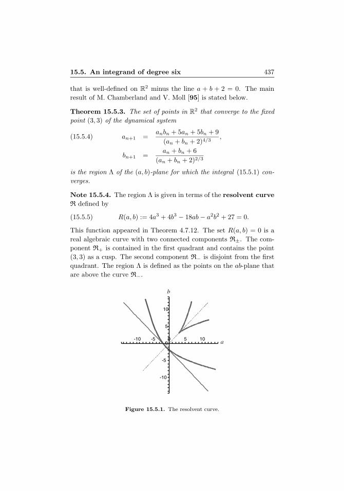
Note 15.5.4. The region Λ is given in terms of the resolvent curve
R defined by
(15.5.5) R(a, b) := 4a3 + 4b3 − 18ab− a2b2 + 27 = 0.
This function appeared in Theorem 4.7.12. The set R(a, b) = 0 is a
real algebraic curve with two connected components R±. The com-
ponent R+ is contained in the first quadrant and contains the point
(3, 3) as a cusp. The second component R− is disjoint from the first
quadrant. The region Λ is defined as the points on the ab-plane that
are above the curve R−.
10
10
5
5
00
-5
-10
-5-10
b
a
Figure 15.5.1. The resolvent curve.
438 15. Landen Transformations
The identity
R(a1, b1) =(a− b)2R(a, b)
(a + b + 2)4(15.5.6)
plays an important role in the dynamics of (15.5.4). In particular it
follows from (15.5.6) that the resolvent curve R(a, b) = 0, and the
regions {(a, b) : R(a, b) > 0}, located between the two branches in
Figure 15.5.1, and {(a, b) : R(a, b) < 0} are preserved by Φ6. The
identity (15.5.6) also shows that the diagonal Δ = {(a, b) : a = b} of
R2 is mapped onto the resolvent curve R. This yields the parametriza-
tion
a(t) =t + 9
24/3(t + 1)1/3and b(t) =
21/3(t + 3)
(t + 1)2/3
of this curve. This parametrization may be employed to analyze the
behavior on the resolvent curve.
Note 15.5.5. The relation between the resolvent curve and the dis-
criminant of a cubic polynomial is clarified in Exercise 4.7.10.
15.6. The original elliptic case
Among the many beautiful results in the theory of elliptic integrals,
a calculation of Gauss stands among the best: take two positive real
numbers a and b, with a > b, and form a new pair by replacing a with
the arithmetic mean (a + b)/2 and b with the geometric mean√ab.
Then iterate:
(15.6.1) an+1 =an + bn
2, bn+1 =
√anbn
starting with a0 = a and b0 = b. K. F. Gauss [133] was interested
in the initial conditions a = 1 and b =√
2. The iteration generates
a sequence of algebraic numbers which rapidly become impossible to
describe explicitly; for instance,
(15.6.2) a3 =1
23
((1 +
4√
2)2 + 2√
28√
2
√1 +
√2
)is a root of the polynomial
G(a) = 16777216a8 − 16777216a7 + 5242880a6 − 10747904a5
+942080a4 − 1896448a3 + 4436a2 − 59840a + 1.
15.6. The original elliptic case 439
The numerical behavior is surprising; a6 and b6 agree to 87 digits. It
is simple to check that
(15.6.3) limn→∞
an = limn→∞
bn.
This common limit is called the arithmetic-geometric mean and
is denoted by AGM(a, b). It is the explicit dependence on the initial
condition that is hard to discover.
Gauss computed some numerical values and observed that
(15.6.4) a11 ∼ b11 ∼ 1.198140235
and then he recognized the reciprocal of this number as a numerical
approximation to the elliptic integral
(15.6.5) I =2
π
∫ 1
0
dt√1 − t4
.
It is unclear to the authors how Gauss recognized this number—he
simply knew it. (Stirling’s tables may have been a help; the book
by J. M. Borwein and D. H. Bailey [69] contains a reproduction of
the original notes and comments.) He was particularly interested in
the evaluation of this definite integral as it provides the length of a
lemniscate. In his diary Gauss remarked, “This will surely open up a
whole new field of analysis.” More details can be found in the book
by J. M. Borwein and P. B. Borwein [71] and the paper by D. Cox
[105].
Gauss’ procedure to find an analytic expression for AGM(a, b)
began with the elementary observation
(15.6.6) AGM(a, b) = AGM
(a + b
2,√ab
)
and the homegeneity condition
(15.6.7) AGM(λa, λb) = λAGM(a, b).
He used (15.6.6) with a = (1+√k)2 and b = (1−
√k)2, with 0 < k < 1,
to produce
AGM(1 + k + 2√k, 1 + k − 2
√k) = AGM(1 + k, 1 − k).
440 15. Landen Transformations
He then used the homogeneity of AGM to write
AGM(1 + k + 2√k, 1 + k − 2
√k)
= AGM((1 + k)(1 + k∗), (1 + k)(1 − k∗))
= (1 + k)AGM(1 + k∗, 1 − k∗),
with
(15.6.8) k∗ =2√k
1 + k.
This resulted in the functional equation
(15.6.9) AGM(1 + k, 1 − k) = (1 + k) AGM(1 + k∗, 1 − k∗).
In his analysis of (15.6.9), Gauss substituted the power series
(15.6.10)1
AGM(1 + k, 1 − k)=
∞∑n=0
ank2n
into (15.6.9) and solved an infinite system of nonlinear equations, to
produce
(15.6.11) an = 2−2n
(2n
n
)2
.
Then he recognized the series as that of an elliptic integral, to obtain
(15.6.12)1
AGM(1 + k, 1 − k)=
2
π
∫ π/2
0
dx√1 − k2 sin2 x
.
This is a remarkable tour de force.
The function
(15.6.13) K(k) =
∫ π/2
0
dx√1 − k2 sin2 x
is the elliptic integral of the first kind. It can also be written in
the algebraic form
(15.6.14) K(k) =
∫ 1
0
dt√(1 − t2)(1 − k2t2)
.
In this notation, (15.6.9) becomes
(15.6.15) K(k∗) = (1 + k)K(k).
15.6. The original elliptic case 441
This is the Landen transformation for the complete elliptic in-
tegral. J. Landen [193], the namesake of the transformation, studied
related integrals: for example,
(15.6.16) κ :=
∫ 1
0
dx√x2(1 − x2)
.
He derived identites such as
(15.6.17) κ = ε√ε2 − π, where ε :=
∫ π/2
0
√2 − sin2 θ dθ ,
proven mainly by suitable changes of variables in the integral for ε.
In the paper by G. N. Watson [307], the reader will find a historical
account of Landen’s work, including the above identities.
The reader will find proofs in a variety of styles in the books by
J. M. Borwein and P. B. Borwein [71] and H. McKean and V. Moll
[213]. In trigonometric form, the Landen transformation states that
(15.6.18) G(a, b) =
∫ π/2
0
dθ√a2 cos2 θ + b2 sin2 θ
is invariant under the change of parameters
(a, b) �→(
a+b2 ,
√ab).
D. J. Newman [235] presents a very clever proof: the change of vari-
ables x = b tan θ yields
(15.6.19) G(a, b) =1
2
∫ ∞
−∞
dx√(a2 + x2)(b2 + x2)
.
Now let x �→ x+√x2 + ab to complete the proof. Many of the above
identities can now be searched for and proven on a computer; see the
book by J. M. Borwein and D. H. Bailey [69].
Note 15.6.1. The reader will find a survey of the many aspects of
Landen transformations in the paper by D. Manna and V. Moll [209].
As an intriguing open problem, the question of producing a Landen
transformation for the integral
U+2 (a, b, c) :=
∫ ∞
0
dx
ax2 + bx + c
remains a challenge.
442 15. Landen Transformations
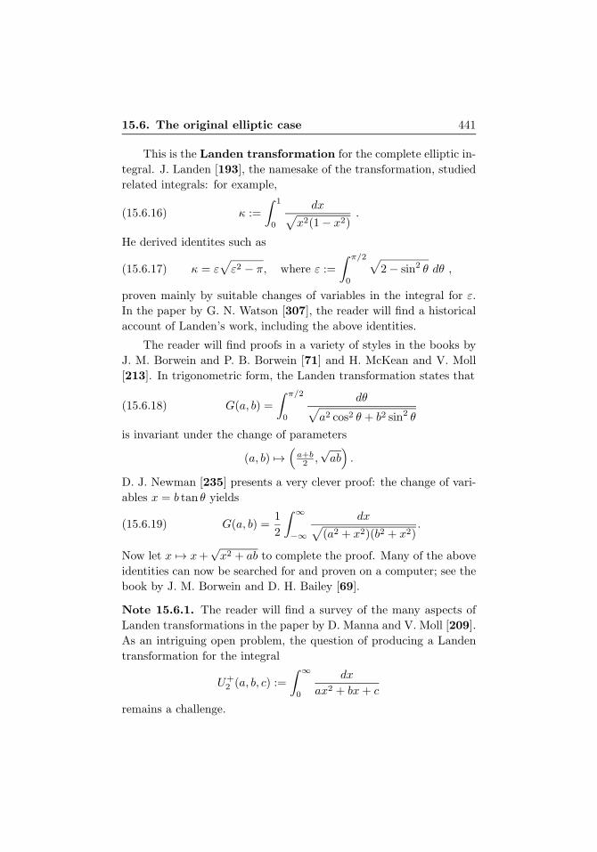
Note 15.6.2. The dynamics of the first two equations in (15.5.2)
with initial data below the resolvent curve is quite complicated. Fig-
ure 15.6.1 shows the first 50000 iterates starting at a = −5.0 and
b = −20.4.
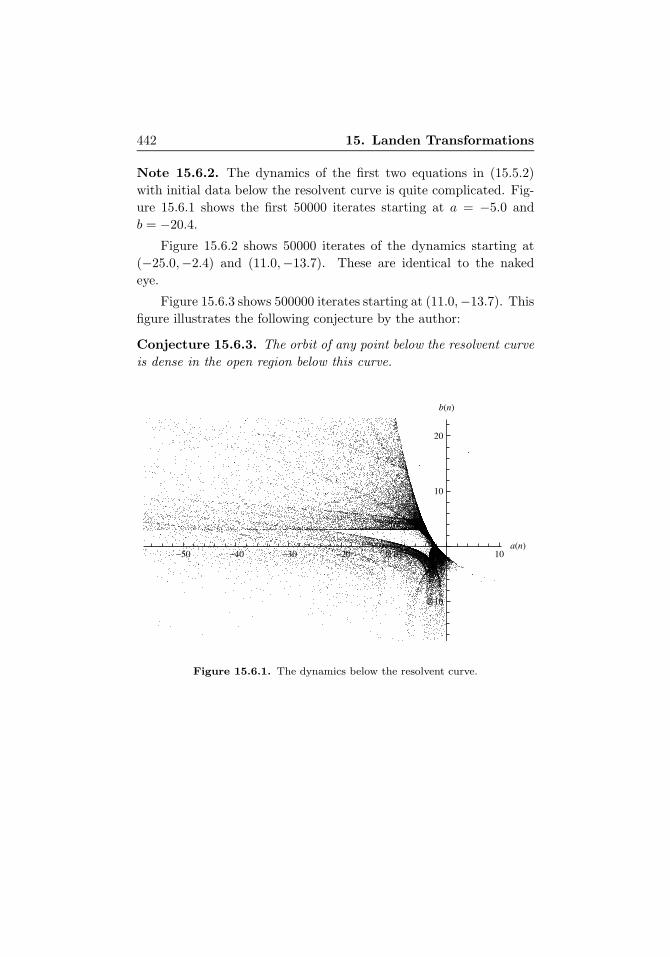
Figure 15.6.2 shows 50000 iterates of the dynamics starting at
(−25.0,−2.4) and (11.0,−13.7). These are identical to the naked
eye.
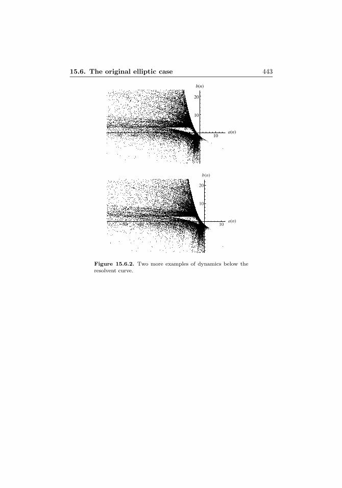
Figure 15.6.3 shows 500000 iterates starting at (11.0,−13.7). This
figure illustrates the following conjecture by the author:
Conjecture 15.6.3. The orbit of any point below the resolvent curve
is dense in the open region below this curve.
10 10a(n)
10
10
20
b(n)
Figure 15.6.1. The dynamics below the resolvent curve.
15.6. The original elliptic case 443
10 10a(n)
10
10
20
b(n)
10a(n)
10
10
20
b(n)
Figure 15.6.2. Two more examples of dynamics below theresolvent curve.
444 15. Landen Transformations
50 40 30 20 10 10a(n)
10
10
20
b(n)
Figure 15.6.3. Illustration of the density conjecture.