Status Report’onNEAMS System’Analysis ... - ipd.anl.gov · About Argonne National Laboratory Argonne is a U.S. Department of Energy laboratory managed by UChicago Argonne, LLC

ANL/NE-‐15/41

Status Report on NEAMS System Analysis Module Development

Nuclear Engineering Division

About Argonne National Laboratory Argonne is a U.S. Department of Energy laboratory managed by UChicago Argonne, LLC under contract DE-AC02-06CH11357. The Laboratory’s main facility is outside Chicago, at 9700 South Cass Avenue, Argonne, Illinois 60439. For information about Argonne and its pioneering science and technology programs, see www.anl.gov.

DOCUMENT AVAILABILITY

Online Access: U.S. Department of Energy (DOE) reports produced after 1991 and a growing number of pre-1991 documents are available free via DOE’s SciTech Connect (http://www.osti.gov/scitech/)

Reports not in digital format may be purchased by the public from the National Technical Information Service (NTIS):

U.S. Department of Commerce National Technical Information Service 5301 Shawnee Rd Alexandria, VA 22312 www.ntis.gov Phone: (800) 553-NTIS (6847) or (703) 605-6000 Fax: (703) 605-6900 Email: [email protected]

Reports not in digital format are available to DOE and DOE contractors from the Office of Scientific and Technical Information (OSTI):

U.S. Department of Energy Office of Scientific and Technical Information P.O. Box 62 Oak Ridge, TN 37831-0062 www.osti.gov Phone: (865) 576-8401 Fax: (865) 576-5728 Email: [email protected]

Disclaimer

This report was prepared as an account of work sponsored by an agency of the United States Government. Neither the United States

Government nor any agency thereof, nor UChicago Argonne, LLC, nor any of their employees or officers, makes any warranty, express

or implied, or assumes any legal liability or responsibility for the accuracy, completeness, or usefulness of any information, apparatus,

product, or process disclosed, or represents that its use would not infringe privately owned rights. Reference herein to any specific

commercial product, process, or service by trade name, trademark, manufacturer, or otherwise, does not necessarily constitute or imply

its endorsement, recommendation, or favoring by the United States Government or any agency thereof. The views and opinions of

document authors expressed herein do not necessarily state or reflect those of the United States Government or any agency thereof,

Argonne National Laboratory, or UChicago Argonne, LLC.

ANL/NE-‐15/41

Status Report on NEAMS System Analysis Module Development

prepared by R. Hu, T.H. Fanning, T. S. Sumner, and Y. Yu Nuclear Engineering Division Argonne National Laboratory December 2015

Status Report on NEAMS System Analysis Module Development R. Hu, T.H. Fanning, T. S. Sumner, and Y. Yu

i ANL/NE-‐15/41

EXECUTIVE SUMMARY

Under the Reactor Product Line (RPL) of DOE-NE’s Nuclear Energy Advanced Modeling and Simulation (NEAMS) program, an advanced SFR System Analysis Module (SAM) is being developed at Argonne National Laboratory. The goal of the SAM development is to provide fast-running, improved-fidelity, whole-plant transient analyses capabilities. SAM utilizes an object-oriented application framework MOOSE), and its underlying meshing and finite-element library libMesh, as well as linear and non-linear solvers PETSc, to leverage modern advanced software environments and numerical methods. It also incorporates advances in physical and empirical models and seeks closure models based on information from high-fidelity simulations and experiments.

This report provides an update on the SAM development, and summarizes the activities performed in FY15 and the first quarter of FY16. The tasks include: (1) implement the support of 2nd-order finite elements in SAM components for improved accuracy and computational efficiency; (2) improve the conjugate heat transfer modeling and develop pseudo 3-D full-core reactor heat transfer capabilities; (3) perform verification and validation tests as well as demonstration simulations; (4) develop the coupling requirements for SAS4A/SASSYS-1 and SAM integration.

The effects of different spatial and temporal discretization schemes are investigated for the updated SAM thermal-fluid models and Components. It is found that the use of 2nd order finite elements would significantly increase the efficiency and accuracy of the simulations. The BDF2 scheme is generally preferred for its second-order accuracy and minimal numerical diffusion for continuous problems; however, backward Euler scheme could be preferred to avoid potential overshooting and undershooting for steep gradient (or discontinuous) problems. The convergence rates of the high-order spatial and temporal discretization schemes have been confirmed by a series of verification tests. It can be concluded that the developed system thermal-hydraulics model can be strictly verified, and that it performs very well for a wide range of flow problems with high accuracy, efficiency, and minimal numerical diffusions.

A pseudo 3-D full-core conjugate heat transfer modeling capability has been developed in SAM for efficient and accurate temperature predictions of structures. The hexagon lattice core can be modeled with 1-D parallel channels representing the subassembly flow, and 2-D duct walls and inter-assembly gaps. A core lattice model is developed to facilitate the generation of all core channels and inter-assembly gaps, as well as the connections among them for user friendliness. The 3-D full-core conjugate heat transfer modeling capability in SAM has been demonstrated by a verification test problem with 7 fuel assemblies in a hexagon lattice layout. The simulation results are compared with RANS-based CFD simulations. Using the two-region core channel model, SAM predictions agree very well with the results from the CFD simulation, while the computational cost is reduced by 6 orders of magnitude.

Validation activities are conducted to assure the performance and validity of the SAM code. The benchmark simulations of two EBR-II tests, an unprotected loss of forced cooling flow test and an unprotected loss of heat rejection test, have been successfully performed. SAS4A/SASSYS-1 simulations were also performed for a code-to-code comparison. These benchmark simulations focused on the thermal-hydraulics responses of the system throughout

Status Report on NEAMS System Analysis Module Development December 2015

ANL/NE-‐15/41 ii

the transients in which the reactor power history was specified in both the SAM and SAS4A/SASSYS-1 models. Very good agreement was found among the two code simulations and the test results for both tests. These results demonstrate that the SAM code can capture the major thermal-hydraulic responses in the primary coolant loop during SFR loss-of-flow and loss-of-heat-sink transients.

Jointly supported by NEAMS and DOE-NE’s Advanced Reactor Technology (ART) program, the coupling scheme and the data exchange for coupling between SAS4A/SASSYS-1 and SAM have been developed. The coupling strategy is similar to the coupling between the core channel thermal-hydraulics models and the PRIMAR-4 coolant system models in SAS4A/SASSYS-1. Several modeling enhancements have been implemented in SAM, including a surrogate core-channel calculation model, and the models needed to account for any discrepancies between the estimated channel flows from the two codes. The next steps will be focused on the implementation of the coupling strategy in both codes, including the data communications and the coupled code execution flow.

Although still in its early stage, the SAM development and the recent progress are very encouraging. It can be confirmed that the major physics phenomena in SFR primary coolant loop during transients can be well captured by SAM simulations, and that the high-order FEM model can significantly improve the code accuracy as well as the efficiency. The next stage of the development will be continued on component designs and physics integration for enhanced modeling capabilities and user experiences, and code verification and validation. Additionally, the integration with other high-fidelity advanced simulation tools developed under the NEAMS Program, such as Proteus, will be investigated to pursue a multi-scale multi-physics simulation using the integrated NEAMS tools. The integration of SAM and SAS4A/SASSYS-1 will also continue in FY16 under the joint support of NEAMS and ART programs.


ANL/NE-‐15/41

TABLE OF CONTENTS

Executive Summary .................................................................................................................... i Table of Contents ...................................................................................................................... iii List of Figures ........................................................................................................................... iv List of Tables ............................................................................................................................ vi 1 Introduction ........................................................................................................................... 1 2 SAM Overview ...................................................................................................................... 3

2.1 Objectives and Development Approach ........................................................................ 3 2.2 Overview of Current Capabilities .................................................................................. 4

3 Updated Verification and Demonstration Simulations .......................................................... 8 3.1 The Effects of Spatial Discretization Scheme ................................................................ 8 3.2 The Effects of Temporal Discretization Scheme ......................................................... 12 3.3 Convergence Verification Tests ................................................................................... 15 3.4 Conclusions .................................................................................................................. 18

4 Demonstration Simulation of Psuedo-3D Full-Core Conjugate Heat Transfer ................... 19 4.1 SAM Multi-Channel Core-Channel Model .................................................................. 19 4.2 Model Description ........................................................................................................ 20 4.3 CFD Simulation Results ............................................................................................... 22 4.4 SAM Simulation Results .............................................................................................. 23 4.5 Conclusions .................................................................................................................. 26

5 Simulation of EBR-II Benchmark Tests .............................................................................. 27 5.1 Model Description ........................................................................................................ 28

5.1.1 Core ................................................................................................................... 28 5.1.2 Coolant System .................................................................................................. 30 5.1.3 Boundary Conditions for Transient Modeling ................................................... 31

5.2 Simulation Results ....................................................................................................... 32 5.2.1 SHRT-45R Results ............................................................................................ 32 5.2.2 BOP-302R Results ............................................................................................. 37

5.3 Conclusions .................................................................................................................. 42 6 Integration with SAS4A/SASSYS-1 ................................................................................... 43

6.1 SAS-SAM Coupling Strategy ...................................................................................... 43 6.2 Data Exchange Requirements ...................................................................................... 45 6.3 SAM Enhancements for Coupling ............................................................................... 46

7 Summary .............................................................................................................................. 49 References ................................................................................................................................ 50


ANL/NE-‐15/41 iv

LIST OF FIGURES

Figure 1: The Structure of the SFR System Analysis Module .................................................... 4 Figure 2: The schematic of the spatial discretization of the core channel problem .................. 10 Figure 3: Errors of fuel centerline temperature predictions of a fuel assembly ........................ 10 Figure 4: Errors of coolant temperature predictions of a fuel assembly ................................... 11 Figure 5: Radial temperature distributions of a heated pin rod ................................................ 12 Figure 6: Transient responses of the pipe under inlet temperature oscillation, BDF2 ............. 14 Figure 7: Damped temperature wave under pipe inlet temperature oscillation, backward

Euler ........................................................................................................................... 14 Figure 8: Smoothing of steep gradient during a temperature step change transient ................. 15 Figure 9: Schematic model of the used fuel assembly cooling test problem ............................ 16 Figure 10: Spatial convergence for steady state natural circulation flow rate .......................... 16 Figure 11: Transient response of the system from forced low to natural circulation, time

step size effects .......................................................................................................... 17 Figure 12: Time convergence of the peak clad temperature in the transient cooling test ........ 18 Figure 13: Region separation in a multi-channel core-channel model ..................................... 20 Figure 14: The 7-assembly computational model (top view) and notations ............................. 21 Figure 15: Duct wall temperature distributions at the core outlet of CFD simulation ............. 22 Figure 16: Coolant temperature distribution at core outlet of assembly 0 and 6 ...................... 23 Figure 17: Axial temperature distributions of the Channel 0 and 6, SAM two-region

model .......................................................................................................................... 24 Figure 18: Radial temperature distributions of the six sides of Channel 0 duct wall, core

outlet .......................................................................................................................... 25 Figure 19: Comparison of average axial wall temperature distributions between SAM and

CFD ............................................................................................................................ 25 Figure 20: Comparison of radial wall temperature distributions between SAM and CFD,

heat structure between Channels 0 and 6 at the core outlet ....................................... 26 Figure 21. SAM Core Channel Model of EBR-II. .................................................................... 29 Figure 22. EBR-II Primary Sodium System Model. ................................................................. 30 Figure 23. Boundary conditions of IHX secondary flow during SHRT-45R test. ................... 31 Figure 24. Normalized pump head history during SHRT-45R test .......................................... 32 Figure 25. Reactor Power and IHX heat removal rate during SHRT-45R test ......................... 34 Figure 26. Pump 2 mass flow rates during SHRT-45R test, Low range .................................. 34 Figure 27. Z-Pipe inlet temperature during SHRT-45R test ..................................................... 35 Figure 28. IHX primary inlet temperature during SHRT-45R test ........................................... 35 Figure 29. Subassembly 6C4 outlet temperature during SHRT-45R test ................................. 36 Figure 30. Peak in-core cladding temperature during SHRT-45R test ..................................... 36 Figure 31. Reactor power and IHX heat removal rate during BOP-302R test ......................... 39


ANL/NE-‐15/41

Figure 32. SAM predictions of plena temperatures during BOP-302R test ............................. 39 Figure 33. High-pressure inlet plenum temperature during BOP-302R test ............................. 40 Figure 34. Low-pressure inlet plenum temperature during BOP-302R test ............................. 40 Figure 35. Z-Pipe inlet temperature during BOP-302R test ..................................................... 41 Figure 36. IHX primary inlet temperature during BOP-302R test ........................................... 41 Figure 37. Subassembly 6C4 outlet temperature during BOP-302R test ................................. 42 Figure 38: Tight Coupling Scheme for a Generic Time Step [24] ............................................ 44 Figure 39: Sequential Two-Way Coupling Scheme for a Generic Time Step .......................... 44 Figure 40: Execution Process Flow Chart of the CoupledSASTransient ................................. 46 Figure 41: Demonstration test problem for SAS-SAM coupling ............................................. 47


ANL/NE-‐15/41 vi

LIST OF TABLES

Table 1. Major SAM Components .............................................................................................. 5 Table 2: ABTR Fuel Assembly Parameters .............................................................................. 20 Table 3. SAM lumped core channels ........................................................................................ 29 Table 4: Data exchange flow for SAS-SAM coupling at the coupling interface ...................... 46

Status Report on NEAMS System Analysis Module Development R. Hu, T.H. Fanning, T. S. Sumner, and Y. Yu 1

ANL/NE-‐15/41

1 Introduction Reactor analyses using system codes are of significant importance to the design, licensing,

and operation of nuclear reactor systems. Many system analysis codes, such as RELAP5 [1], CATHARE [2] and SAS4A/SASSYS-1 [3], have been developed since the early 1970s and successfully applied for the design, license, and operational analysis of the nuclear power plants. Although these codes have achieved a high level maturity, they have not taken full advantage of the rapid expansion in computing power and advances in numerical methods over the past two decades.

With advances in numerical techniques and software engineering, there has been a renewed interest in the advanced system code developments such as RELAP-7 [4] and CATHARE-3 [5] for advanced physical and numerical modeling of two-phase flows. Research in high-order numerical schemes for system simulation of two-phase flow is also of increasing interest [6][7]. Under the U.S. Department of Energy (DOE) Nuclear Energy Advanced Modeling and Simulation (NEAMS) program, a system analysis module (SAM) [8][9] is being developed at Argonne National Laboratory for advanced reactor system analysis. It focuses on the modeling of the components and systems that represent typical features of advanced reactor concepts such as SFRs (sodium fast reactors), LFRs (lead-cooled fast reactors), and FHRs (fluoride-salt-cooled high temperature reactors). These advanced concepts are distinguished from light-water reactors in their use of single-phase, low-pressure, high-temperature, and low Prandtl number (sodium and lead) coolants. This simple yet fundamental change has significant impacts on core and plant design, the types of materials used, component design and operation, fuel behavior, and the significance of the fundamental physics in play during transient plant simulations.

The goal of the SAM development is to provide user-friendly fast-running, improved-fidelity whole-plant transient analyses capabilities. SAM utilizes an object-oriented application framework MOOSE [10], and its underlying meshing and finite-element library libMesh [11], as well as linear and non-linear solvers PETSc [12], to leverage modern advanced software environments and numerical methods. It incorporates advances in physical and empirical models and seeks closure models based on information from high-fidelity simulations and experiments. Additionally, coupling interfaces have been developed to allow for convenient integration with other advanced or conventional simulation tools for multi-scale and multi-physics modeling capabilities.

This report provides an update of the SAM developments in FY15 and the first quarter of FY16. An overview of the code development approach and the current capabilities is provided in Section 2.

In FY15, all SAM Components were updated to support 2nd-order finite elements for both improved accuracy and computational efficiency. Section 3 discusses the efficiency of the high-order elements, the effects of the spatial and temporal discretization schemes, and the results from related verification tests. Additionally, verification test problems are presented to confirm the high-order numerical convergence rates.

A flexible conjugate heat transfer modeling capability is also implemented in SAM in FY15. In Section 4, the 3-D full-core conjugate heat transfer modeling capability is demonstrated by a verification test problem with 7 fuel assemblies in a hexagon lattice layout.

Status Report on NEAMS System Analysis Module Development 2 December 2015

ANL/NE-‐15/41

The simulation results are compared with the RANS-based CFD simulation using the commercial CFD code STAR-CCM+ [13]. Good agreements have been achieved between the results of the two approaches.

As an important part of code development, validation activities are being conducted to assure the performance and validity of the SAM code. Section 5 presents the benchmark simulations of two EBR-II tests[14], an unprotected loss of forced cooling flow test (SHRT-45R) and an unprotected loss of all heat rejection test (BOP-302R). The code predictions of major primary coolant system parameter are compared with the test results. Additionally, the SAS4A/SASSYS-1 code simulation results are also included for a code-to-code comparison.

Section 6 discusses the coupling scheme and the data exchange for coupling between SAS4A/SASSYS-1 and the SAM. This effort is jointly support by NEAMS and DOE-NE’s Advanced Reactor Technology (ART) program. The goal is to combine the advantages in both codes, and to provide a modern code framework to support enhanced modeling capabilities that are not currently possible.

Finally, Section 7 provides a summary of the current status on SAM development and the direction needed for future code development work.


ANL/NE-‐15/41

2 SAM Overview

2.1 Objectives and Development Approach SAM is being developed as a system-level modeling and simulation tool with improved

accuracy while remaining computationally efficient. It will provide user-friendly, fast-running, improved-fidelity, whole-plant transient analyses capabilities. These capabilities are essential for the fast turnaround design scoping and engineering analyses, and could lead to improvements in the design of new reactors, the reduction of uncertainties in safety analysis, and reductions in capital costs.

The SAM code structure is shown in Figure 1. To leverage the available advanced software environments and numerical methods, SAM utilizes an object-oriented application framework (MOOSE), the underlying meshing and finite-element library (LibMesh), as well as the non-linear solvers (PETSc). It also incorporates advances in physical and empirical models and seeks closure models based on information from high-fidelity simulations and experiments.

As a new code development, the initial effort focused on developing modeling and simulation capabilities of the heat transfer and single-phase fluid dynamics responses in the SFR systems. SAM employs a one-dimensional transient model for single-phase incompressible but thermally expandable flow. The governing equations consist of the continuity, momentum, and energy equations. A three dimensional module is also under development to model the multi-dimensional flow and thermal stratification in the upper plenum or the cold pool in the SFR reactor vessel. Additionally, a subchannel module will be developed for more-detailed fuel assembly modeling. The details of the one-dimensional single-phase flow model for incompressible thermally expandable flow and the stabilization schemes can be found in Ref. [15]. Heat structures in SAM model the heat conduction inside the solids and permit the modeling of convective heat transfer at the interfaces between solid and fluid components. Heat structures can represent one-dimensional or two-dimensional heat conduction in Cartesian or cylindrical coordinates. Temperature-dependent thermal conductivities and volumetric heat capacities can be provided in tabular or functional form either from built-in or user-supplied data. The modeling capabilities of heat structures can be used to predict the temperature distributions in solid components such as fuel pins or plates, heat exchanger tubes, and pipe and vessel walls, as well as to calculate the heat flux conditions for fluid components. A flexible conjugate heat transfer modeling capability is implemented in SAM, and the details can be found in Ref. [16].

The physics modeling (fluid flow and heat transfer) and mesh generation of individual reactor components are encapsulated as Component classes in SAM along with some component specific models. A set of components has been developed based on the FEM fluid model and heat conduction model, including: (1) basic fluid and solid geometric components; (2) 0-D components for setting boundary conditions; (3) 0-D components for connecting 1-D components; (4) assembly components by combining the basic geometric components and the 0-D connecting components; and (5) non-geometric components for physics integration.

Additionally, coupling interfaces have been developed to allow for convenient integration with other advanced or conventional simulation tools for multi-scale and multi-physics modeling capabilities. Multi-scale multi-physics analyses by adopting the combined use of


ANL/NE-‐15/41

different computational tools are vital for many practical nuclear engineering applications. For example, coupled system thermal-hydraulics and CFD code simulations are important for reactor safety analyses when three-dimensional effects play an important role in the evolution of a given transient or accident scenario, which was demonstrated in the coupled SAM and STAR-CCM+ code simulation of the SFR protected-loss-of-flow transient [9]. The integrations of SAM with the other advanced tools in NEAMS and with the conventional SFR safety tool SAS4A/SASSYS-1 are currently under development.

Figure 1: The Structure of the SFR System Analysis Module

2.2 Overview of Current Capabilities To develop a system analysis code, numerical methods, mesh management, equations of

state, fluid properties, solid material properties, neutronics properties, pressure loss and heat transfer closure laws, and good user input/output interfaces are all indispensible. SAM leverages the MOOSE framework and its dependent libraries to provide JFNK solver schemes, mesh management, and I/O interfaces while focus on new physics and component model development for the SFR systems.

A numerically stable scheme for continuous finite element analysis of single-phase flow and heat transfer has been developed for non-LWR advanced reactor applications. The primitive variable (or pressure) based formulation, in which the state variables are pressure (𝑝), velocity (𝑢), and temperature (𝑇), is developed and implemented in SAM. The primitive variable based FEM formulation is more suitable for incompressible or nearly incompressible flows, such as the fluid flow in the SFRs, LFRs, or FHRs. To prevent potential numerical instability issues, the stabilization techniques of incompressible flows were extensively reviewed, and the Streamline-Upwind Petrov-Galerkin (SUPG) and the Pressure-Stabilizing

!

SAM!

MOOSE!

Fundamental*Physics*Models*

Component*Physics*Integra8on*

Mul89Scale*Mul89Physics*Integra8on*

STAR9CCM+*SHARP*

SAS4A/SASSYS91*…*

Suppor8ng*Elements*


ANL/NE-‐15/41

Petrov-Galerkin (PSPG) formulations [17] have been chosen and implemented as the stabilization schemes. Major SAM Components are listed in Table 1. Most of them have been developed in FY14. The transient simulation capabilities of typical SFR accidents have been demonstrated in a number of reactor transient simulations [9]. In FY15, all SAM Components were updated to support 2nd-order finite elements (Edge3 in 1-D or Quad-9 in 2D) for both improved accuracy and computational efficiency. The developed physics models and components provide several major modeling features:

1. One-D pipe networks to represent general fluid systems such as the reactor coolant loops;

2. Flexible integration of fluid and solid components, able to model complex and generic engineering system. A general liquid flow and solid structure interface model was developed for easier implementation of physics models in the components.

3. A pseudo three-dimensional capability by physically coupling the 1-D or 2-D components in a 3-D layout. For example, the 3-D full-core heat-transfer in an SFR reactor core can be modeled. The heat generated in the fuel rod of one fuel assembly can be transferred to the coolant in the core channel, the duct wall, the inter-assembly gap, and then the adjacent fuel assemblies.

4. SFR (pool-type) specific features such as liquid volume level tracking, cover gas dynamics, heat transfer between 0-D pools, fluid heat conduction, etc. These are important features for accurate SFR safety analysis.

Table 1. Major SAM Components Component name Descriptions Dimension

PBOneDFluidComponent Simulates 1-D fluid flow using the primitive variable formulation 1-D

HeatStructure Simulates 1-D or 2-D heat conduction inside solid structures 1-D or 2-D

PBCoupledHeatStructure The heat structure connecting two liquid components (1-D or 0-D). 1-D or 2-D

PBPipe Simulates the fluid flow in a pipe and the heat conduction in the pipe wall.

1-D fluid, 1-D or 2-D

structure

PBHeatExchanger

Simulates a heat exchanger, including the fluid flow in the primary and secondary sides, convective heat transfer, and heat conduction in the tube wall.


structure

PBCoreChannel

Simulates reactor core channels, including 1-D flow channel and the inner heat structure of the fuel rod, and the outer heat structure of the duct wall.


structure


ANL/NE-‐15/41

PBDuctedCoreChannel Simulates reactor core channels with an outer heat structure of the duct wall.


structures

PBBypassChannel Models the bypass flow in the gaps between fuel assemblies. 1-D

FuelAssembly

Models reactor fuel assemblies composed of multiple CoreChannels, representing different regions of a fuel assembly (core, gas plenum, reflector, shield, etc.).


structure

DuctedFuelAssembly Model reactor fuel assemblies composed of multiple DuctedCoreChannels.


structure

MultiChannelRodBundle Model the rod bundle with a multi-channel model, in which multiple CoreChannels and HeatStructures are defined and created.


structure

ReactorCore Models a pseudo three-dimensional reactor core; It consists of member core channels (with duct walls) and bypass channels.

Non-D

HexLatticeCore Describes a hexagonal lattice core, in which the CoreChannels and HeatStructures are configured and created.

Non-D

PipeChain A non-geometric component for connecting a number of fluid components. Non-D

PBBranch Models a zero-volume flow joint, where multiple 1-D fluid components are connected. 0-D

PBSingleJunction Models a zero-volume flow joint, where two 1-D fluid components are connected. 0-D

PBPump Simulates the pump component, in which the pump head is dependent on a pre-defined function.

0-D

PBVolumeBranch

Considering the volume effects of a flow joint so that it can account for the mass and energy in-balance between the inlets and outlets due to inertia

0-D

CoverGas A 0-D gas volume that is connected to one or multiple liquid volumes. 0-D

PBLiquidVolume The 0-D liquid volume with cover gas, thus the liquid volume can change during the transient. 0-D

StagnantVolume

A 0-D liquid volume with no connections to 1-D fluid components, but allow for heat transfer with heat structures and mixing with other 0-D volumes.

0-D


ANL/NE-‐15/41

PBTDJ An inlet boundary in which the flow velocity and temperature are provided by pre-defined functions.

0-D

PBTDV A boundary in which the pressure and temperature conditions are provided by pre-defined functions.

0-D

CoupledTDV A TDV boundary in which the boundary conditions are provided by other codes in coupled code simulation.

0-D

CoupledVolumeBranch A PBVolumeBranch component with connecting flow conditions from an external code in coupled code simulation.

0-D

CoupledPBLiquidVolume A PBLiquidVolume component with connecting flow conditions from an external code in coupled code simulation.

0-D


ANL/NE-‐15/41

3 Updated Verification and Demonstration Simulations SAM Components were updated to support 2nd-order finite elements for improved

accuracy and computational efficiency. High order spatial and high-order time discretization schemes have been applied to solve the one-dimensional fluid flow and heat transfer. The effects of different spatial and temporal discretization schemes are investigated in this Section. Additionally, a series of verification test problems are presented to confirm the high-order schemes.

3.1 The Effects of Spatial Discretization Scheme The general residual form of the governing equations discussed above can be written as:

𝑅 𝑈 = !"!"+ ∇𝐹 − 𝑆 = 0 (1)

and the weak form (in FEM) can be derived by multiplying a vector of test functions 𝑊, integrating over the domain Ω, and applying the Gaussian divergence theorem,

!"!"∙𝑊 − 𝐹 ∙ ∇𝑊 − 𝑆 ∙𝑊 𝑑Ω+ (𝐹 ∙𝑊 ) ∙ 𝑛𝑑𝛤!! = 0 (2)

in which the first term represents the volume integral and the second term represents the boundary surface integral. The approximate problem then proceeds by selecting test functions, which is spanned by the basis {𝜙!}. In SAM, the continuous Galerkin formulation is used (through MOOSE and LibMesh); therefore the same shape functions are used for both the trial and test functions, and the unknowns can be expressed in the same basis used for the test functions, i.e.

𝑈 ≈ 𝑈! = 𝑈!𝜙!! (3)

∇𝑈 ≈ ∇𝑈! = 𝑈!∇𝜙!! (4)

SAM uses Lagrange polynomials for both the test functions and the shape functions (sometimes called trial functions). Therefore, these coefficients 𝑈! actually comprise the solution vector 𝑈 at each node.

Substituting the expansions (Eq.-7 and Eq.-8) back into the weak form, we get:

!!!

!"∙ ψ! − 𝐹 ∙ ∇𝜓! − 𝑆 ∙ 𝜓! 𝑑Ω+ (𝐹 ∙ 𝜓! ) ∙ 𝑛𝑑𝛤!! = 0

(5)

The left-hand side of the equation above is generally referred as the 𝑖!! component of the “Residual Vector” and writes as 𝑅!(𝑈!).

In SAM, both linear elements (EDGE2 and QUAD4) and the second-order elements (EDGE3 and QUAD9) are available for use in the finite-element discretization of a reactor system. For first-order elements using piece-wise linear Language shape functions, the trapezoidal rule is recommended for the numerical integration; while the Gaussian quadrature rule is recommended for second-order elements (with second-order Language shape functions) in SAM. In one-D analysis,


ANL/NE-‐15/41

Trapezoidal rule: 𝑓 𝑥 𝑑𝑥!! = (𝑏 − 𝑎) [! ! !!(!)]

! (6)

Gaussian quadrature rule: 𝑓(𝑥)𝑑𝑥!! = 𝑓 𝑥!" 𝑤!"!" (7)

In which 𝑥!" is the quadrature point, and 𝑤!" is the weight. In SAM, the Gauss-Legendre quadrature is used (through MOOSE and LibMesh); and the quadrature points and weights are well defined.

In One-Dimension, Trapezoid formula with an interval h gives error of the order 𝑂(ℎ!). On the other hand, the Gaussian quadrature rule can exactly integrate polynomials of order 2𝑛 − 1 with 𝑛 quadrature points. However, the error can be difficult to estimate as it depends on the 2𝑛 order derivative. The error bound [18] is,

𝐸𝑟𝑟𝑜𝑟 = 𝑓(𝑥)𝑑𝑥!! − 𝑓 𝑥!" 𝑤!" =!"

!!! !!!! !! !

!!!! !! ! !𝑓 !! 𝜉 , 𝑎 < 𝜉 < 𝑏. (8)

It can be concluded that SAM spatial discretization scheme is at least second-order accurate with the first-order elements, and could have exponential convergence rates with the second-order elements for continuous problems.

Here, a core channel problem (coolant flow and solid conduction in fuel assembly) with uniform power distribution inside the fuel pin is presented to confirm its efficiency. The schematic of the spatial discretization of the core channel problem is shown in Figure 2. The different lines of colors on the left represent different heat structures in an SFR fuel pin (i.e., fuel, sodium gap, and clad). Note that each element between two nodes represents a first-order 1-D finite element. If an extra node is added in the center of the element, it becomes a second-order element. The fluid and solid domains exchange energy at the fluid-structure interface nodes. The inlet of the core channel flow is fixed at constant temperature and flow rate. Constant material thermophysical properties are assumed for this verification test. Therefore, the analytical solutions of this test problem can be easily derived, with coolant temperature:

𝑇!""#$%& 𝑧 = 𝑇!" +!!

!!!𝑧 (9)

and the fuel centerline temperature:

(10)

Both 1st order element and 2nd order element schemes were applied for this test problem. The errors between the code predictions and the analytical solutions are shown in Figure 3 and Figure 4 for fuel centerline temperatures and coolant temperatures, respectively. It is clearly seen that the errors from 2nd order elements simulation are essentially zero, even though only two radial elements were used for the fuel pellet region. However, the errors from 1st order element simulation remained notable when using 20 radial elements to model the fuel pellet.

!!_!" ! = !!" + !! !!

!!!! +1

2!!!!!" !ℎ! +1

2!!!!! !"!!"!!"

+1

2!!!!! !ℎ! +1

4!!!!! !


ANL/NE-‐15/41

Figure 2: The schematic of the spatial discretization of the core channel problem

Figure 3: Errors of fuel centerline temperature predictions of a fuel assembly

0

0.2

0.4

0.6

0.8

1

1.2

1.4

1.6

1.8

2

0 0.1 0.2 0.3 0.4 0.5 0.6 0.7 0.8

Fuel Cen

terline

Tem

perature Errors (K)

Axial PosiVon (m)

p1, n=20

p2, n=2

1D flow

1D or 2D structure

r

z

q’’’

q”


ANL/NE-‐15/41

Figure 4: Errors of coolant temperature predictions of a fuel assembly

Another test problem is also examined to verify the efficiency of using 2nd finite-elements. A solid cylinder (2cm diameter) is heated with uniform volumetric power density inside. A constant temperature is assumed on the outer surface. The analytical radial temperature distribution can be easily derived as a quadratic function since constant material thermophysical properties are assumed.

𝑇 𝑟 = 𝑇! +!!!!!(!!!!!!)

!!

(11)

In which 𝑇! is the outer surface temperature, and 𝑟! is the radius of the cylinder. Again, both 1st order elements and 2nd order elements were applied for this test problem. The radial temperature distributions from various spatial discretizations are shown in Figure 5. It is seen that errors still exists with 40 radial elements if using 1st order shape function, while no errors were observed even with a single radial element if using 2nd order shape function.

0

0.05

0.1

0.15

0.2

0.25

0.3

0.35

0 0.1 0.2 0.3 0.4 0.5 0.6 0.7 0.8

Coolan

t Tem

perature Errors (K)

Axial PosiVon

p1, n=20

p2, n=2


ANL/NE-‐15/41

Figure 5: Radial temperature distributions of a heated pin rod

3.2 The Effects of Temporal Discretization Scheme SAM, through MOOSE, supports a number of standard time integration methods such as

the explicit Euler, implicit Euler (or backward Euler), and BDF2 (backward differentiation formula – 2nd order) method, Crank-Nicolson, and Runge-Kutta methods. For most reactor applications, we recommend to use the implicit Euler or BDF2 methods with SAM.

The backward differentiation formula (BDF) is a family of implicit methods for the numerical integration of ordinary differential equations. They are linear multistep methods that, for a given function and time, approximate the derivative of that function using information from already computed times, thereby increasing the accuracy of the approximation. Note that the first order method of this family, BDF1, is equivalent to the backward Euler method. For a time-step-size ∆𝑡, applying the BDF methods to the ordinary differential equation:

!"!"= 𝑓(𝑢, 𝑡) (12)

would result in:

𝑓 𝑢!!!, 𝑡!!! = !!!!!!!

∆!+ 𝑂(∆𝑡), Backward Euler or BDF1;

𝑓 𝑢!!!, 𝑡!!! =!!!

!!!!!!!!!!!!!!

∆!+ 𝑂(∆𝑡!), BDF2.

(13)

Which shows that SAM temporal discretization can be second-order accurate when using the BDF2 scheme.

One challenging problem for traditional system codes, such as TRACE and RELAP-5, is to accurately model the wave oscillation or the sudden disturbance of the system without any numerical instability and numerical diffusion concerns due to their first-order approximations of the differential equations in both time and space. An example of the density wave propagation is presented here in a pipe flow problem. The inlet temperature of a one-meter pipe oscillates following a sinusoidal distribution, 𝑇!"(𝑡) = 628+ 100 ∗ 𝑠𝑖𝑛 (𝜋𝑡); the inlet

600

620

640

660

680

700

720

0 0.005 0.01

Tempe

rature (K

)

Radial PosiVon (m)

p1n10 p1n20 p1n40 p2n1 p2n2

700

701

702

703

704

705

706

707

708

709

0 0.0005 0.001 0.0015 0.002 0.0025

Tempe

rature (K

)

Radial PosiVon (m)

p1n10 p1n20 p1n40 p2n1 p2n2


ANL/NE-‐15/41

velocity is fixed, 𝑢!" 𝑡 = 0.5 𝑚/𝑠; and the initial pipe temperate is at 628 K. The transient responses of the wave propagation are shown in Figure 6, where the code predictions agreed very well with the analytical solutions. This is because of the high-order accuracy in both spatial and temporal (BDF2) discretizations in SAM. If the first-order time integration scheme (backward Euler) were used, numerical damping or diffusion would occur, as shown in Figure 7.

Another challenging problem, generally true for all types of numerical analyses, is the modeling of the non-continuity (steep gradient). A steep gradient problem is tested again in a simple pipe flow. The inlet temperature of the pipe follows a step function, and the inlet velocity is fixed 𝑢!" 𝑡 = 1 𝑚/𝑠.

𝑇!" 𝑡 = 628 𝐾, 𝑖𝑓 𝑡 ≤ 0728 𝐾, 𝑖𝑓 𝑡 > 0 (14)

The transient responses of the temperature step change are shown in Figure 8, in which results from both backward Euler (BDF1) and BDF2 schemes are included. The smoothing of the temperature gradient over time is clearly observed in both schemes. The overshooting of temperature predictions was resulted at the jump with the BDF2 scheme. This is a known issue for the BDF2 scheme to model the steep gradient problems. One the other hand, the Backward Euler scheme requires much smaller time step sizes (𝑑𝑡 = 0.001𝑠) to achieve similar diffusion comparing to the BDF2 scheme (𝑑𝑡 = 0.01𝑠 ) for this test problem. Therefore, the BDF2 seems to be the better choice if efficiency is more important, while the backward Euler would be better if accuracy is more important for steep gradient problems. It should be also noted that the smoothing could be acceptable since: (1) some physical diffusions (molecule diffusion, turbulence, conduction) are real, but commonly neglected in the 1-D flow formulation; and 2) further refining the mesh and reducing the time-step size would reduce the smoothing or damping.


ANL/NE-‐15/41

Figure 6: Transient responses of the pipe under inlet temperature oscillation, BDF2

Figure 7: Damped temperature wave under pipe inlet temperature oscillation, backward Euler

520$

570$

620$

670$

720$

0$ 0.2$ 0.4$ 0.6$ 0.8$ 1$

Tempe

rature)(K

))

Axial)Posi4on)(m))

t=0s$t=0.5s$t=1s$t=1.5s$t=2s$


ANL/NE-‐15/41

Figure 8: Smoothing of steep gradient during a temperature step change transient

3.3 Convergence Verification Tests Verification of the numerical convergence rates is an essential part of the modern software

verification and validation process. To verify the accuracy of the SAM code on spatial discretization, a series of tests are presented here on the natural convection cooling of a used fuel assembly. In this test problem, the used SFR fuel assembly sits in a large sodium pool, and the decay heat level is assumed to be 0.4% (~48 hours after reactor shutdown) of the peak fuel assembly in ABTR[19]. Equal pressure boundary conditions (𝑃! = 10! 𝑃𝑎) are assumed at the inside and outside of the top of the fuel assembly, as seen in Figure 9.

Both 1st order elements and 2nd order elements were applied for this test problem. The errors in the predicted steady-state natural circulation flow rates from various spatial discretizations are shown in Figure 10. Since the analytical solution is very difficult to obtain, the result of the case using 40 2nd-order elements for each fluid component was used as the reference solution. The second order accuracy in spatial discretization is clearly demonstrated from the error trendline for the cases using 1st order elements. The accuracy of 2nd order elements is more difficult to obtain, since the results is already very accurate with the coarsest spatial representations (5 elements per fluid component), and the errors due to the settings of convergence criteria would interfere the errors due to spatial discretization.

To verify the accuracy of the SAM code on temporal discretization, the above test problem was slightly modified. The inlet pressure of the downward flow outside the assembly was assumed at a slightly higher pressure (like a pressure head provided by a pump) at steady state, 𝑃! = 1.1×10! 𝑃𝑎. At 𝑡 = 1𝑠, the pressure is suddenly reduced to the assembly outlet pressure (10! 𝑃𝑎 ). This transient simulates the transition from forced flow to natural

620$

640$

660$

680$

700$

720$

740$

760$

0$ 0.2$ 0.4$ 0.6$ 0.8$ 1$

Tempe

rature)(K

))

Axial)Posi4on)(m))

t=0.05s,$Backward$Euler$t=0.75s,$Backward$Euler$t=0.05s,$BDF2$t=0.75s,$BDF2$t=0.05s,$Analy?cal$t=0.75s,$Analy?cal$


ANL/NE-‐15/41

circulation flow in cooling the used fuel assembly. In this study of temporal convergence, the spatial discretization scheme of 40 2nd-order elements for each fluid component is used. The transient responses of core flow rates and peak clad temperatures (PCT) are shown in Figure 11. It is seen that the system approached the final steady state of natural circulation cooling after 200 seconds. The errors in the predicted PCTs from various time step sizes using the BDF2 scheme are shown in Figure 12. The result of the case using the smallest time step size (0.2s) was used as the reference solution since the analytical solution is not available. The convergence rate of the time step size is seen about 2nd order from the trendline.

Figure 9: Schematic model of the used fuel assembly cooling test problem

Figure 10: Spatial convergence for steady state natural circulation flow rate

y = 37.336x-‐2.01

0

0.2

0.4

0.6

0.8

1

1.2

1.4

1.6

0 10 20 30 40 50

Error in Flow

Rate Pred

icVo

n (%

)

Element Number

Flow Error, P1

Flow Error, P2

Trendline, P1

P0 , T0

P0


ANL/NE-‐15/41

(a) Core flow rate

(b) Peak Clad Temperature

Figure 11: Transient response of the system from forced low to natural circulation, time step size effects

!0.5%

0%

0.5%

1%

1.5%

2%

2.5%

3%

3.5%

4%

0% 50% 100% 150% 200% 250% 300%

Flow

%Rate%(kg/s)%

Time%(s)%

dt=2s%dt=1s%dt=0.5s%dt=0.2s%

630$

640$

650$

660$

670$

680$

690$

0$ 50$ 100$ 150$ 200$ 250$ 300$

Peak%Clad%Tempe

rature%(K

)%

Time%(s)%

dt=2s$

dt=1s$

dt=0.5s$

dt=0.2s$


ANL/NE-‐15/41

Figure 12: Time convergence of the peak clad temperature in the transient cooling test

3.4 Conclusions The effects of different spatial and temporal discretization schemes are investigated for

the updated SAM thermal-fluid models and Components. It is found that the use of 2nd order finite elements would significantly increase the efficiency and accuracy of the simulations. The BDF2 scheme is generally preferred for its second-order accuracy and minimal numerical diffusion for continuous problems; however, backward Euler scheme could be preferred to avoid potential overshooting and undershooting for steep gradient (or discontinuous) problems. Additionally, the convergence rates of the high-order spatial and temporal discretization schemes have been confirmed by a series of verification tests. It can be concluded that the developed system thermal-hydraulics model can be strictly verified, and that it performs very well for a wide range of flow problems with high accuracy, efficiency, and minimal numerical diffusions.

y = 1.2652x2.4309

1.0E-‐01

1.0E+00

1.0E+01

0 0.5 1 1.5 2 2.5

PCT Error (K)

Time Step Size (s)

PCT Error

Trendline


ANL/NE-‐15/41

4 Demonstration Simulation of Psuedo-‐3D Full-‐Core Conjugate Heat Transfer One important design requirement for SFRs is the knowledge of the temperature on the

hexagonal ducts for a thermo-mechanical analysis. This is particular important to ensure the passive safety of the reactor under the unprotected accident conditions if the reactor control system fails to function and the reactivity feedback from structural deformation such as core radial expansion is significant. This information requires a good evaluation of the inter-assembly flow and heat transfer in this region. The physical phenomena are particularly complicated and require a reliable modeling of the whole core including the inter-assembly region.

For efficient and accurate temperature predictions of sodium fast reactor structures, a 3-D full-core conjugate heat transfer modeling capability is developed in SAM. The hexagon lattice core is modeled with 1-D parallel channels representing the subassembly flow, and 2-D duct walls and inter-assembly gaps. The six sides of the hexagon duct wall are modeled separately to account for different temperatures and heat transfer between inner assembly flow and each side of the duct wall. A core lattice model is developed to facilitate the generation of all core channels and inter-assembly gaps, as well as the connections among them for user friendliness. The 3-D full-core conjugate heat transfer modeling capability in SAM has been demonstrated by a verification test problem with 7 fuel assemblies in a hexagon lattice layout. Additionally, the simulation results are compared with a RANS-based CFD simulation.

4.1 SAM Multi-‐Channel Core-‐Channel Model To improve the heat transfer between the duct wall and coolant flow, a multi-channel core

channel model is developed in SAM to account for the temperature differences between the center region and the edge region of the coolant channel in a fuel assembly. For a regular triangular lattice pin bundle, the flow area, heated and wetted perimeters, and the equivalent hydraulic and heated diameters of all regions are well defined, as shown in Figure 13. In the SAM multi-channel model, all fluid regions are modeled as separate pipes with the same pressure drop and no net mass exchange. However, the heat exchange is possible at all axial nodes between two adjacent channels, and the energy exchange rate is modeled as:

!!!"= 𝛽(𝜌𝑣)!"#𝑆(ℎ! − ℎ!) (15)

in which, 𝛽 is the mixing parameter (accounting for both turbulent mixing and directional flow); (𝜌𝑣)!"# is the average mass flux between Region 1 and 2; 𝑆 the total gap width between Channel 1 and 2; and ℎ! and ℎ! are the enthalpies of Channel 1 and 2.


ANL/NE-‐15/41

Figure 13: Region separation in a multi-channel core-channel model

4.2 Model Description A 7-assembly model has been developed to examine the pseudo 3-D full-core conjugate

heat transfer modeling capability in SAM. The fuel assembly geometry is based on the Advanced Burner Test Reactor (ABTR) conceptual design [19], and the major parameters of the ABTR fuel assembly design are listed in Table 2.

Table 2: ABTR Fuel Assembly Parameters

Assembly Parameters Pin number 217

Assembly pitch (m) 0.14598 Duct outside flat-to-flat distance (m) 0.14198

Duct inner flat-to-flat distance (m) 0.13598 Assembly duct thickness (m) 0.003

Inter-assembly gap width (m) 0.004 Assembly length (m) 0.8

Pin Parameters Pin diameter (m) 0.008

Pin pitch-to-diameter ratio 1.13 Pin pitch (m) 0.00904


ANL/NE-‐15/41

Seven identical fuel assemblies of 217 pins each are modeled in this study. The System Thermal-Hydraulics (STH) and the CFD models of this 7-assembly problem are shown in Figure 14. In the SAM model, it is modeled with 1-D parallel channels representing the subassembly flow, and 2-D structures representing the duct walls and the inter-assembly sodium gaps. Note that a two-region model is used for all 7 assemblies and the 6 sides of the hexagon duct wall are modeled separately to account for different temperatures and heat transfer between inner assembly flow and each side of the duct wall. The red dots in Figure 14a represent the center fluid channels of the seven assemblies. The green dots represent the edge fluid channels. Finally, the blue lines represent the fuel pins, the heat structures between two assemblies (including two duct wall widths and the inter-assembly sodium gap), and the duct wall sides with adiabatic boundary conditions on the outside surface. For simplicity, the inter-assembly flow in the gap is neglected in this work, and only heat conduction is considered. A CFD model is also developed for comparison, as seen in Figure 14b. For simplicity (in the CFD simulation), only bare-bundle simulations were performed in this code-to-code benchmark exercise, and constant thermophysical properties of the sodium and duct wall are used in this work.

In the 7-assembly model, it is assumed that the center assembly (Channel 0) has higher power density with power peaking factor of 1.5, and that the lower-right assembly (Channel 6) has lower power density with power peaking factor of 0.5. All the other assemblies have the same power density with power peaking factor of 1. Uniform power distributions (both radial and axial) are assumed within each assembly. Additionally, the same inlet flow rate is applied for all assemblies.

(a) STH model (b) CFD model

Figure 14: The 7-assembly computational model (top view) and notations

Name rule: Number: assemble position (0~6) Alphabet: wall position (a, b, c, d, e, f)


ANL/NE-‐15/41

4.3 CFD Simulation Results Realizable k-ε turbulence model, the two-layer all-y+ wall formulation, and segregated

flow solver with the SIMPLE predictor-corrector algorithm are used in the CFD simulation. The solution is well converged as the normalized residuals are below 10-4. Figure 15 presents the temperature distributions at the core outlet of the 7-assembly CFD simulation. It is seen that the hot and cold assemblies significantly affected the duct wall temperatures of the neighbor assemblies. However, the effect diminishes with increasing distance from neighbor assembly ducts to these two assemblies.

The coolant temperature distributions at the core outlet of Assembly 0 and 6 from the CFD simulation are shown in Figure 16. It is seen that the edge region of the two assemblies are much colder than the inner regions. Similar findings were also found in the authors’ previous work on CFD simulations of wire-wrapped fuel assemblies. It is also confirmed that the temperature of duct wall 6C is higher than the coolant temperature near the wall in the CFD simulation; therefore, the coolant of Assembly 6 is receiving heat from the wall 6C, although its average coolant temperature is higher than the wall.

(a) Duct walls and assembly gap temperature distribution

(b) Between assembly #0 and #3 (c) Between assembly #0 and #6

Figure 15: Duct wall temperature distributions at the core outlet of CFD simulation

0~6

3~0

6 0

0 3


ANL/NE-‐15/41

(a) Assembly 0 (b) Assembly 6 Figure 16: Coolant temperature distribution at core outlet of assembly 0 and 6

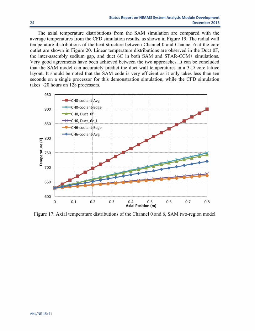
4.4 SAM Simulation Results A two-region model is used for all 7 assemblies in the SAM simulation. Based on an

energy balance calculation using the CFD simulation results, it is found that the energy exchange between the inner and edge zones is very small comparing to the heating power in each zone for the 7-assembly test problem. Therefore, 𝛽 = 0 was assumed in the SAM analysis of this demonstration problem.

The axial temperature distributions of the Channel 0 and 6 from the SAM two-region model simulation are shown in Figure 17. Note that the temperature differences between the inner wall and the edge coolant are the same for Channel 0 and 6, indicating the convective heat transfer is balanced at the two sides of the inter-assembly heat structures. It is seen that the inner wall temperature of Duct 6C is lower than the average coolant temperature of Channel 6, but higher than the edge coolant temperature, as has been observed in the CFD simulation. In the two-region model, Zone 2 (edge region) has lower power density (for the total volume of pin and coolant regions), but higher mass flux (due to the larger hydraulic diameter and less friction coefficient). Therefore, its temperature would be much lower than that of Zone 1 (inner region).

The radial temperature distributions of the six sides of Channel 0 duct wall at the core outlet are shown in Figure 18. It is seen the temperature of Duct 0F is significantly lower than the other sides, as it faced the lower power Channel 6. The temperature differences among the other 5 sidewalls are negligible. This is because the inter-assembly heat transfer is very small compared to the heating power from the fuel rod, and the 5 average-power assemblies have almost the same coolant temperature predictions despite their positions relative to the high- or low-power assembly. For the center high-power assembly, the total heat removal between coolant and the six sides of the duct is ~22.5 kW, which is only ~0.3% of the heating power (7.58 MW).


ANL/NE-‐15/41

The axial temperature distributions from the SAM simulation are compared with the average temperatures from the CFD simulation results, as shown in Figure 19. The radial wall temperature distributions of the heat structure between Channel 0 and Channel 6 at the core outlet are shown in Figure 20. Linear temperature distributions are observed in the Duct 0F, the inter-assembly sodium gap, and duct 6C in both SAM and STAR-CCM+ simulations. Very good agreements have been achieved between the two approaches. It can be concluded that the SAM model can accurately predict the duct wall temperatures in a 3-D core lattice layout. It should be noted that the SAM code is very efficient as it only takes less than ten seconds on a single processor for this demonstration simulation, while the CFD simulation takes ~20 hours on 128 processors.

Figure 17: Axial temperature distributions of the Channel 0 and 6, SAM two-region model

600

650

700

750

800

850

900

950

0 0.1 0.2 0.3 0.4 0.5 0.6 0.7 0.8

Tempe

rature (K

)

Axial PosiVon (m)

CH0-‐coolant-‐Avg

CH0-‐coolant-‐Edge

CH0, Duct_0f_I

CH6, Duct_6c_I

CH6-‐coolant-‐Edge

CH6-‐coolant-‐Avg


ANL/NE-‐15/41

Figure 18: Radial temperature distributions of the six sides of Channel 0 duct wall, core outlet

Figure 19: Comparison of average axial wall temperature distributions between SAM and

CFD

710

715

720

725

730

735

740

745

750

0 0.5 1 1.5 2 2.5 3

Wal Tem

perature (K

)

Radial PosiVon (mm)

Side A Side B Side C Side D Side E Side F

600

620

640

660

680

700

720

740

760

0 0.1 0.2 0.3 0.4 0.5 0.6 0.7 0.8

Tempe

rature (K

)

Axial PosiVon (m)

CH0_f_I, CFD

CH6_c_I, CFD

CH0_f_I, SAM

CH6_c_I, SAM


ANL/NE-‐15/41

Figure 20: Comparison of radial wall temperature distributions between SAM and CFD, heat

structure between Channels 0 and 6 at the core outlet

4.5 Conclusions A pseudo 3-D full-core conjugate heat transfer modeling capability has been developed in

SAM for efficient and accurate temperature predictions of SFR structures. The hexagon lattice core is modeled with 1-D parallel channels representing the subassembly flow, and 2-D duct walls and inter-assembly gaps. The six sides of the hexagon duct wall are modeled separately to account for different temperatures and heat transfer between inner assembly flow and each side of the duct wall. A core lattice model is developed to facilitate the generation of all the core channels and inter-assembly gaps, as well as the connections among them for user friendliness.

The 3-D full-core conjugate heat transfer modeling capability in SAM has been demonstrated by a verification test problem with 7 fuel assemblies in a hexagon lattice layout. The simulation results are compared with RANS-based CFD simulations. It was found that a lumped coolant channel model (one temperature per axial position) would significantly overestimate the duct wall temperatures. Instead, a two-region core channel model is required to accurately model the duct wall temperature and inter-assembly heat transfer. Using the two-region model, SAM predictions agree very well with the results from the CFD simulation, while the computational cost is reduced by 6 orders of magnitude. This demonstrates that the SAM can efficiently and accurately model the inter-assembly heat transfer and the duct wall temperatures in a 3-D core lattice layout.

670

680

690

700

710

720

730

740

750

0 1 2 3 4 5 6 7 8 9 10

Tempe

rature

Radial PosiVon (mm)

CFD

SAM


ANL/NE-‐15/41

5 Simulation of EBR-‐II Benchmark Tests The EBR-II plant was a 62.5 MWth metallic fueled sodium fast reactor designed and

operated between 1964 and 1994 by Argonne National Laboratory. During its operation, EBR-II was used for experiments designed to demonstrate the feasibility of passive safety in liquid metal reactors (LMR). The Shutdown Heat Removal Test program was carried out in EBR-II between 1984 and 1986. The objectives of the program were to support the U.S. advanced LMR program, provide test data for validation of computer codes, and demonstrate passive reactor shutdown and decay heat removal in response to protected and unprotected transients. Through an ongoing effort under DOE-NE’s Advanced Reactor Technology (ART) program, some of the EBR-II test data are recovered and organized into electronic databases.

Argonne has performed analyses of SHRT-17 and SHRT-45R, the most severe protected and unprotected loss of flow tests, using SAS4A/SASSYS-1 under an ongoing four-year International Atomic Energy Agency (IAEA) coordinated research project [20][21]. The benchmark specifications of the EBR-II tests are also being used to support code validation efforts during SAM development. Preliminary SHRT-17 benchmark simulation results were presented in Ref. [9]. Major physics phenomena in the primary coolant loop during the protected-loss-of-flow transients were well captured in the SAM simulation. This paper presents the benchmark simulations of SHRT-45R and an unprotected loss of all heat rejection test, BOP-302R.

The SHRT-45R test was conducted to demonstrate the effectiveness of inherent feedback mechanisms in EBR-II to terminate the fission process. Starting from full power and flow, SHRT-45R was initiated by simultaneously tripping both the primary and intermediate-loop coolant pumps to simulate an unprotected loss-of-flow accident. Once the loss of flow transient began, forced convection flow continued while the pumps coasted down. After the pumps had stopped, the flow transitioned to natural circulation. The system then relied upon natural circulation to remove residual heat from the core. During the test, the plant protection system (PPS) was disabled to prevent a scram. Temperatures in the reactor quickly rose to high, but acceptable levels as the inherent reactivity feedbacks reduced the fission power. SHRT-45R demonstrated that natural phenomena such as thermal expansion of reactor materials could be effective in protecting the reactor against potentially adverse consequences from unprotected loss-of-flow accidents.

The BOP, or balance of plant, tests were a series of tests performed during the SHRT testing program to investigate transients where the primary sodium pumps did not trip. A variety of different BOP tests were performed ranging from tests where the control rod insertion depth fluctuated to other tests where the intermediate sodium electromagnetic pump was oscillated at various frequencies. BOP-302R was one of two loss-of-heat-sink tests where the intermediate sodium pump was tripped without scramming the control rods or tripping the primary pumps. This test was driven by increasing core inlet temperatures, which were a result of a diminished IHX heat rejection rate due to the lower intermediate sodium flow rates. BOP-302R was performed several hours after SHRT-45R and was initiated from full power and full flow.


ANL/NE-‐15/41

5.1 Model Description An EBR-II model, similar to the SAS4A/SASSYS-1 model described in Ref. [21], was

developed for SHRT-45R and BOP-302R benchmark simulations, as shown in Figures 21 and 22. To simplify the input preparation, minor flow leakages are not modeled.

5.1.1 Core The thermal-hydraulic performance of a reactor core is analyzed in SAM with a model

consisting of a number of core channels. The channel model provides input to specify a single fuel pin and its associated coolant and structure. A single-pin channel represents the average pin in an assembly, and assemblies with similar reactor physics and thermal-hydraulic characteristics are grouped together.

Five single-pin channel types were created for the driver, partial driver, dummy, reflector, and blanket assemblies. The SHRT-45R and BOP-302R core models use 12 channels based on one of these five channel types to represent all 637 subassemblies. The safety, experimental, and control subassemblies are not modeled with their own channel types but rather are grouped into other channels. The same core model was used for both SHRT-45R and BOP-302R tests. Table 3 and Figure 21 illustrate the channels in the EBR-II core model. Among them, six channels (with six different colors in Figure 21) represent: (1) the lumped fuel assembly groups of the driver fuel assemblies; (2) the high-flow driver fuel assemblies; (3) lumped channel for all dummy (K-type), partial driver (P-type), experimental, and control assemblies; (4) inner core reflector assemblies; (5) outer core reflector assemblies; and (6) blanket assemblies. Another six channels shown in red represent six individual assemblies with different types at locations 1A1, 2B1, 4C3, 6C4, 7A3, and 12E6. These subassemblies were modeled individually because they were among a subset of subassemblies whose outlet temperatures were measured. A 22-channel model is used in SAS4A/SASSYS-1, and the details can be found in Ref. [21].

Reactivity feedbacks are not modeled in these benchmark simulations as some important reactivity feedback mechanisms, such as the radial and axial core expansion, control rod drive line expansion, etc., can not yet be modeled in SAM. Instead, the reactor power histories from the tests are directly applied in the simulation of the transients. Although these reactivity feedback mechanisms can be modeled in SAS4A/SASSYS-1, the same assumptions were used in both simulations for consistent comparisons of the thermal-hydraulics responses of the system throughout the transients.


ANL/NE-‐15/41

Table 3. SAM lumped core channels Channel number Representations Total Assembly

number Total Power

(MW) Total Flow

(kg/s) 1 Average Driver 56 33.7 232 2 Average High Flow Driver 18 10.3 67.5

3 Lumped Channel, K+X+P+Control 28 8.66 77.3

4 Average Inner Reflector 20 0.278 3.32 5 Average Outer Reflector 180 0.855 11.2 6 Average Blanket 329 4.50 64.5 7 1A1, Half-Driver 1 0.332 3.81 8 2B1, K016 1 0.0177 0.685 9 4C3, Driver 1 0.692 4.86

10 6C4, Driver 1 0.598 3.71 11 7A3, Reflector 1 0.0149 0.165 12 12E6, Blanket 1 0.0268 0.163

Total 637 60.0 469

Figure 21. SAM Core Channel Model of EBR-II.

Channel 1: Driver

Channel 2: High Flow Driver

Channel 3: K-Type, P-Type, Experimental, and Control

Channel 4: Inner Reflector

Channel 5: Outer Reflector

Channel 6: Blanket

Channel 7-12: Six Individual Assemblies


ANL/NE-‐15/41

5.1.2 Coolant System Figure 22 illustrates the EBR-II primary system model used in the SAS4A/SASSYS-1

simulations. A similar model is used in the SAM simulations except that the minor flow leakage paths were not modeled. The two primary pumps draw sodium from the cold pool and feed the high- and low-pressure flow paths. Sodium flows through the high-pressure inlet piping (e.g. E14èE15èE16) and is discharged into the high-pressure inlet plenum before flowing up through the inner core channels. Sodium flowing through the low-pressure inlet piping (e.g. E17èE18èE19èE20èE21) is discharged into the low-pressure inlet plenum before flowing up through the outer core channels. The inner core channels represent the first seven rows of subassemblies and the outer core channels represent the remaining subassemblies in rows 8-16. At steady state, the mass flow rates through the inner core and outer core subassemblies are approximately 390 kg/s and 70 kg/s, respectively.

The inner and outer core channels both discharge into the outlet plenum, which mixes the discharged sodium before it enters the Z-Pipe. The Z-Pipe is a double-walled pipe that contains the auxiliary EM pump. Sodium leaving the Z-Pipe flows through the intermediate heat exchanger before discharging into the cold pool.

Figure 22. EBR-II Primary Sodium System Model.

Pum

p #1

Pum

p #2

High-PressureInlet PlenumCV1

Low-PressureInlet PlenumCV2

Low-PressureInlet PlenumCV2

Outlet PlenumCV3

Inner CoreS1E1

Outer CoreS2E2

Outer CoreS2E2

CV5 CV6

Byp

ass

S3

E3

S14E36

S13E35

S12E34

S11E33

E22E11

S4

E4

E5

E6 E7

S5 S8

S6 S9

S7 S10E14

E15

E16

E25

E26

E27

E12

E23

E13 E24

E17

E18

E19

E20

E21

E28

E29

E30

E31

E32

IHX

Upper Cold PoolCV4

E9

E10

Lower Cold PoolCV7

E8

S15E37


ANL/NE-‐15/41

5.1.3 Boundary Conditions for Transient Modeling As discussed above, the benchmark simulation focused on the thermal-hydraulics

responses of the system throughout the transients in which the reactor power history was specified as input to the models for both SAM and SAS4A/SASSYS-1.

The complete intermediate loop was also not modeled in the benchmark tests. Instead, the IHX intermediate side inlet temperatures and mass flow rates are provided as boundary conditions. A simplified pump model is used in SAM for both tests in which the pump speed history during the tests are directly applied. Figures 23 and 24 shows the IHX secondary conditions and the primary pump heads during the SHRT-45R test.

Figure 23. Boundary conditions of IHX secondary flow during SHRT-45R test.

0"

0.2"

0.4"

0.6"

0.8"

1"

1.2"

544"

546"

548"

550"

552"

554"

556"

558"

560"

562"

0" 200" 400" 600" 800"Normalized

+IHX+Second

ary+Flow

+Rate+

IHX+Second

ary+Inlet+T

empe

rature+(K

)+

Time+(s)+

IHX"Secondary"Inlet"Temperature"

IHX"Secondary"Flow"Rate"


ANL/NE-‐15/41

Figure 24. Normalized pump head history during SHRT-45R test

5.2 Simulation Results

5.2.1 SHRT-‐45R Results Simulation results of the SHRT-45R test are shown in Figures 25-30. The reactor core

power and the instantaneous heat removal rate of the IHX are shown in Figure 25. This transient is initiated by a complete loss of forced coolant flow in the primary and intermediate loops. The two primary pumps are designed with sufficient rotating inertia to maintain rotation until about 50 seconds after the start of the transient. This is followed by a transition to natural circulation. Immediately after the transient is initiated, the reactor temperature increases and the reactor power is slowly reduced due to various reactivity feedback mechanisms. After about 150 seconds, the reactor core power became lower than the IHX heat removal rate. This is expected since fair amounts of flow were remained for the intermediate heat transport system (IHTS) during SHRT-45R test. At the end of the 900-second test, the IHTS flow is still about 8% of the normal flow rate.

Figure 26 shows that the transition to natural circulation flow is very smooth. The transient response of the primary loop flow in the simulation is very close to that of the experiment and the SAS4A/SASSYS-1 simulation results, although the magnitudes are slightly different during the transition from forced flow to natural circulation flow. This is deemed successful considering the delicate coupling among the natural circulation flow, the friction and form losses, and the temperature distribution of the whole system.

!0.2%

0%

0.2%

0.4%

0.6%

0.8%

1%

0% 100% 200% 300% 400% 500% 600% 700% 800% 900%

Normalized

+Pum

p+He

ad+

Time+(s)+

Aux.%Pump%Main%Pump%1%Main%Pump%2%


ANL/NE-‐15/41

Because the primary vessel is so large, the cold pool temperature does not change much during SHRT-45R. This leads to rather flat high-and low-pressure inlet plena temperature profiles. Both high- and low-pressure inlet plenum temperatures decrease several degrees during the test, likely due to over-cooling by the IHX through the later part of the transient.

The Z-Pipe inlet temperature is shown in Figure 27. The transient responses of the core outlet temperatures in the simulation are very similar to the experiment. The rapid flow decrease during the early part of the transient results in an increase of the core outlet and then the Z-Pipe inlet temperature. Core power decreases rapidly due to various reactivity feedback mechanisms. Once the natural circulation flow is fully established and because the IHX heat removal is higher than the core power, the core outlet and Z-Pipe inlet temperatures start dropping. The Z-Pipe inlet temperature rises faster in both SAM and SAS4A/SASSYS-1 simulations than the measured data because the upper plenum is modeled as a zero-dimensional volume. However, complex geometry and flow patterns existed in the EBR-II core outlet plenum. There is a delay as hotter sodium enters the volume, flows through or around the baffle plate, and enters the Z-Pipe, but it cannot be modeled in a 0-D volume. The Z-Pipe inlet temperature from the SAM simulation is slightly over-predicted in the second half of the test, possibly due to the differences in the modeling of heat transfer between the upper plenum and the shield walls.

The IHX primary inlet temperature response during the transient is shown in Figure 28. Very large differences are found between both code predictions and the measurements while the two code predictions are very similar. Because the IHX inlet temperature thermocouple was installed inside the IHX along the outer surface of a tube, not at the inlet where higher flow mixing is expected, it is speculated that the IHX inlet thermocouple did not measure the average temperature of sodium leaving the Z-Pipe. The IHX inlet temperature is also significantly affected by the Z-Pipe heat loss due to the longer transit time in the Z-Pipe under low flow transient conditions. Figures 27 and 28 show that the IHX inlet temperature is significantly lower than the Z-Pipe inlet temperature during the transient, although it is only 1.5°C lower than the Z-Pipe inlet temperature under the steady state full flow conditions.

The core outlet temperature of driver fuel subassembly 6C4, highest power-to-flow ratio among all channels, is shown in Figure 29. The transient trends among the experiment and the two simulations are very similar, but the peak core outlet temperatures are different. It is suspected that there is a gap between the subassembly outlet and the temperature measurement location. Under low flow conditions, the mixing between the subassembly 6C4 and the adjacent low power subassemblies would reduce the core outlet temperature measurement in the test. The peak cladding temperatures from the SAM and SAS4A/SASSYS-1 simulations through the SHRT-45R test are shown in Figure 30. Almost identical results are found although different core channel groupings and different friction and form loss models are used. It can be confirmed that major fluid flow and heat transfer responses in the primary coolant loop during the unprotected loss-of-flow test can be captured by both the SAM and SAS4A/SASSYS-1 codes.


ANL/NE-‐15/41

Figure 25. Reactor Power and IHX heat removal rate during SHRT-45R test

Figure 26. Pump 2 mass flow rates during SHRT-45R test, Low range

0.E+00

1.E+07

2.E+07

3.E+07

4.E+07

5.E+07

6.E+07

7.E+07

0 200 400 600 800

Pow

er (W

)

Time (s)

IHX heat removal

Reactor power


ANL/NE-‐15/41

Figure 27. Z-Pipe inlet temperature during SHRT-45R test

Figure 28. IHX primary inlet temperature during SHRT-45R test


ANL/NE-‐15/41

Figure 29. Subassembly 6C4 outlet temperature during SHRT-45R test

Figure 30. Peak in-core cladding temperature during SHRT-45R test


ANL/NE-‐15/41

5.2.2 BOP-‐302R Results BOP-302R was a loss of heat sink test where the intermediate sodium pump was tripped

without scramming the control rods or tripping the primary pumps. This test was driven by increasing core inlet temperatures, which were a result of the diminished IHX heat rejection due to the lower intermediate sodium flow rates. Strong thermal stratification is expected in the primary vessel (cold pool), where the IHX outlet and the pump inlets are located in the upper part of the vessel. To correctly predict the core inlet temperature, the thermal stratification in the cold pool needs to be properly considered. This is accounted for in the SAM simulation with a two-volume pool model, in which the upper volume connects with the main primary pumps and the IHX, and the lower volume is stagnant but the mixing flow with the upper volume and the convective heat transfer with the immersed piping walls are considered. Similar modeling approaches were also applied in the SAS4A/SASSYS-1 model.

The StagnantVolume component is developed in SAM to model a stagnant volume with no connections to any 1-D fluid components, but allowing for heat transfer with other 0-D volumes or heat structures. For simplicity, it is assumed that the mass of the stagnant volume is unchanged. Only the energy conservation is needed for the stagnant volume component:

!(!")!"

+ 𝑄!!!!! = 0 (16)

In which, 𝑀: the total mass of the component; 𝐻: the average enthalpy of the component. 𝑡: time; 𝑛: the number of coupling heat transfer components; 𝑄: heat transfer with coupled heat structures or 0-D volumes; 𝑄 = ℎ!"#$∆𝑇 𝑑𝐴 for heat transfer with heat structures; 𝑄 = 𝑚!"#∆ℎ for heat transfer with 0-D volumes, and 𝑚!"# is the mixing flow rate with the coupling 0-D volume. In the SAM BOP-302R simulation, the mixing flow between the upper and lower cold pool is assumed to be 50% of the primary core flow rate.

Simulation results of the BOP-302R test are shown in Figures 31-37. Very good agreement was found among the SAM and SAS simulations and the test results. This demonstrates that both the SAM and SAS codes can capture the major thermal-hydraulic responses in the primary coolant loop during the unprotected loss-of-heat-sink test.

The reactor core power and the instantaneous heat removal rate of IHX are shown in Figure 31. As discussed above, this transient is initiated by a complete loss of forced coolant flow in the intermediate loop, which resulted in a diminished IHX heat rejection rate. The reactor power is slowly reduced due to various reactivity feedback mechanisms. Throughout the transient, the reactor power is always higher than the IHX heat removal rate. For a short period, the IHX secondary side temperature is higher than the primary side, which results in heat transfer from the intermediate loop to the primary loop.

SAM predictions of the plena temperatures during BOP-302R test are shown in Figure 32. The upper cold pool temperature increases rapidly at the beginning of the transient due to the loss-of-cooling in the IHX. As the primary loop coolant flow rate is largely unchanged throughout the transient, the core outlet plenum temperature drops with the decrease of the core power. As the IHX primary outlet temperature decreases and the continuous mixing between the upper and lower cold pool, the upper cold pool temperature decreases eventually after reaching a peak. The temperature responses in the high- and low-pressure core inlet plena are similar to the upper cold pool, and the temperature at the low-pressure inlet plenum is slightly lower due to the heat loss to the lower cold pool through the long piping. The lower


ANL/NE-‐15/41

cold pool temperature response is much slower compared to other volumes, as it does not directly participate in the primary coolant flow loop. Eventually all plena temperatures became very close to each other as the lower cold pool was heated up.

The comparisons of high- and low-pressure inlet plena temperatures from the SAM and SAS simulations and the test results are shown in Figure 33 and Figure 34. Very good agreement was achieved for both the initial heat up rates and the later pseudo-equilibrium states. It is demonstrated that the thermal stratification in the cold pool during the test can be modeled with a relatively simple multiple 0-D volume model. Note that the mixing flow rates between 0-D volumes are crucial to accurately model the heat transfer between 0-D volumes, and the mixing flow rates can be derived from RANS-based CFD simulations of the system at several different primary loop flow rates.

The Z-Pipe inlet and IHX primary inlet temperature responses are shown in Figure 35 and Figure 36. As the primary loop coolant flow rate is largely unchanged at full flow, the coolant temperature rise across the reactor core is very small. The core outlet temperature continues dropping as the reactor power decreases. The Z-Pipe inlet and IHX primary inlet temperature responses follow the same response. This is expected because the heat loss through the Z-Pipe walls is negligible during high flow conditions. Very good agreement was found among the two code simulations and the test results.

The core outlet temperature of the driver fuel subassembly 6C4 is shown in Figure 37. The transient trends among the experiment and the two simulations are very similar, but the initial increase of core outlet temperature was not observed in the test results. It is suspected again that the mixing between the subassembly 6C4 and the adjacent low power subassemblies reduced its outlet temperature measurement in the test. Very similar results are found between the SAM and SAS simulations.


ANL/NE-‐15/41

Figure 31. Reactor power and IHX heat removal rate during BOP-302R test

Figure 32. SAM predictions of plena temperatures during BOP-302R test

-2.E+06

0.E+00

2.E+06

4.E+06

6.E+06

8.E+06

1.E+07

0 900 1800 2700 3600 4500

Pow

er (W

)

Time (s)

IHX Heat Removal

Reactor Power

600

620

640

660

680

700

720

740

0 1000 2000 3000 4000

Tem

pera

ture

(K)

Time (s)

High pressure inlet plenum

Low pressure inlet plenum

Upper plenum

Upper cold pool

Lower cold pool


ANL/NE-‐15/41

Figure 33. High-pressure inlet plenum temperature during BOP-302R test

Figure 34. Low-pressure inlet plenum temperature during BOP-302R test


ANL/NE-‐15/41

Figure 35. Z-Pipe inlet temperature during BOP-302R test

Figure 36. IHX primary inlet temperature during BOP-302R test


ANL/NE-‐15/41

Figure 37. Subassembly 6C4 outlet temperature during BOP-302R test

5.3 Conclusions Validation activities are being conducted to assure the performance and validity of the

SAM code. The benchmark simulations of two EBR-II tests, unprotected loss of forced cooling flow test (SHRT-45R) and unprotected loss of heat rejection test (BOP-302R), have been successfully performed. These benchmark simulations focused on the thermal-hydraulics responses of the system throughout the transients in which the reactor power history was specified in both the SAM and SAS4A/SASSYS-1 models. Very good agreement was found between the two code simulations and the test results for both tests. For the SHRT-45R test, the transient response of the primary loop flow in the SAM simulation agreed very well with the experiment during the whole transient, which went through the forced-flow during the pump coast-down, transition flow, and the natural circulation flow regimes. For the BOP-302R test, the high- and low-pressure inlet plena temperatures from SAM simulations agreed very well with the test for both the initial heat up rates and the later pseudo-equilibrium states, which demonstrated that the thermal stratification in the cold pool was correctly accounted for by the simple two-volume cold pool model. These results demonstrate that the SAM code can capture the major thermal-hydraulic responses in the primary coolant loop during SFR loss-of-flow and loss-of-heat-sink transients.


ANL/NE-‐15/41

6 Integration with SAS4A/SASSYS-‐1 SAS4A/SASSYS-1 is a simulation tool used to perform deterministic analysis of

anticipated events as well as design basis and beyond design basis accidents for advanced liquid-metal-cooled nuclear reactors. With its origin in the late 1960s, the SAS series of codes has been under continuous use and development for over forty-five years and represents a critical investment in safety analysis capabilities and user experience for the U.S. Department of Energy. SAS4A/SASSYS-1 plays a significant role in a number of U.S. Department of Energy programs as well as domestic and international collaborations. Modernization and extension of the code system is an on-going process sponsored by the DOE-NE Office of Advanced Reactor Technology, with recent developments documented in References [22] and [23].

To combine the advantages of SAS4A/SASSYS-1 and SAM, an initial coupling strategy has been defined that retains the full complement of core (in the reactor sense) modeling capabilities of SAS4A/SASSYS-1 — coolant channel and sub-channel thermal hydraulics, sodium boiling, fuel restructuring and relocation, in-pin fuel melting, cladding failure, and fuel and clad melting and relocation — and adds the option to use SAM for the primary, intermediate, and decay heat coolant systems. In the planned approach, the primary and intermediate system modeling capabilities of SAS4A/SASSYS-1 will be retained to maintain continuity of simulation capabilities.

6.1 SAS-‐SAM Coupling Strategy In all multi-code coupling applications, careful controls of data exchange and time

synchronization are essential for a numerically stable and physically valid simulation [24]. When using a tight coupling scheme, an interface consistency, or convergence, check is needed to make sure the results are consistent at the coupling interface between two codes, as shown in Figure 38. If this scheme were adopted, each time step is repeated in both SAM and SAS4A/SASSYS-1 until the desired convergence is achieved. Tight coupling in this manner usually does not require significant modifications to the underlying solution schemes of the two codes. However, this approach often requires the modification of the time stepping control in the two codes, which is not always a trivial task. In SAS4A/SASSYS-1, for example, a multi-level time-step hierarchy is used to ensure stability of the many different accident models available. The SAS4A/SASSYS-1 primary and intermediate system modeling component, PRIMAR-4, uses a theta-weighted, semi-implicit solution scheme with time-step cutback controls to avoid expensive iterations. Therefore, a tight coupling scheme that requires iteration may not be appropriate.

Instead, a sequential two-way coupling scheme will be used for coupling SAM with SAS4A/SASSYS-1. This approach is shown in Figure 39. In this scheme, each of the two codes drives its own portion of the simulation and coupling interface data is exchanged at well-defined points. For steady-state initialization, SAS4A/SASSYS-1 will determine core inlet and outlet boundary conditions based on model input. Those conditions will provide the initial steady-state conditions for SAM. During the transient, the roles will be reversed. SAM will determine coolant system dynamic changes, such as loss of flow or loss of heat sink, and will define the interface conditions for the core channel models in SAS4A/SASSYS-1.


ANL/NE-‐15/41

Figure 38: Tight Coupling Scheme for a Generic Time Step [24]

Figure 39: Sequential Two-Way Coupling Scheme for a Generic Time Step

This approach is similar to the proven approach used between the SAS4A/SASSYS-1 core channel models and PRIMAR-4. In PRIMAR-4, a surrogate core channel model is used to estimate the rate of change in the mass flow rate for each channel. Additionally, the differences between the estimated channel flows and computed channel flows are considered in the adjustments of the plena coupling parameters. In this way, the numerical stability of the coupled code is assured, while the modifications of SAS4A/SASSYS-1 are minimized.

SAM$

SAS$

Interface$data$from$SAS$to$SAM$at$tn01$

Interface$data$from$SAS$to$SAM$for$tn+1$

Internal$itera5ons$

Time$Step$N$

Interface$Convergence$

Yes$

No$

Data$from$SAM$to$SAS$at$tn$

Interface$data$from$SAS$at$tn$


ANL/NE-‐15/41

6.2 Data Exchange Requirements In SAS4A/SASSYS-1, the multi-channel core model is coupled with PRIMAR-4 at the

inlet and outlet plenums. When the core-channel thermal hydraulics module in SAS4A/SASSYS-1 completes a time step for the core simulation portion of the transient, it also defines a surrogate models for each channel. The surrogate models are used during the PRIMAR-4 time step to approximate changes in core channel flow rates during the next primary coolant system time step.

The surrogate models are defined based on the following equation that relates changes in the core channel flow rates to changes in the plenum pressures:

𝑑𝑤𝑑𝑡 = 𝐶! − 𝐶!𝑝in + 𝐶!𝑝out + 𝐶!𝑤 𝑤 (17)

The coefficients 𝐶! through 𝐶! are provided by the core channel model to PRIMAR-4, while the pressure and flow variables are solved by PRIMAR-4 during the primary coolant time step. Solutions for pressure and flow are estimates because they are based on the surrogate model.

For transients in which the core channel coolant remains single phase, these estimates will be quite accurate. If boiling initiates, the process of void formation and coolant expulsion introduce rapid, non-linear changes that require significant reductions in time-step sizes in order to maintain accuracy. Also, PRIMAR-4 will need to adjust plenum mass, pressure, temperature, and cover-gas interface elevations to account for differences between the estimated channel flows based on the linear surrogate model and the actual flows computed by the coolant dynamics models.

Following completion of a time step for the primary and intermediate coolant loops, PRIMAR-4 provides the following information back to the core channel coolant dynamics routines in SAS4A/SASSYS-1:

𝑝in 𝑡! = inlet plenum pressure at the beginning of the PRIMAR-4 time step

𝑝out 𝑡! = outlet plenum pressure at the beginning of the PRIMAR-4 time step

𝑑𝑝in𝑑𝑡 ,

𝑑𝑝out𝑑𝑡 = time derivatives of the inlet and outlet plenum pressures

𝑇in,𝑇out = inlet and outlet plenum temperatures

These parameters provide the boundary conditions needed to update the core channel solution. The plan for this work is to utilize a similar coupling method with SAM. The data

exchange between the two codes at each coupling interface (core channel/plenum) is summarized in Table 4.


ANL/NE-‐15/41

Table 4: Data exchange flow for SAS-SAM coupling at the coupling interface SAS → SAM (at the beginning of SAM time step)

For every channel: 𝐶!, 𝐶!, 𝐶!, and 𝐶! Mass Flow Rate Inlet and Outlet Temperature

SAM → SAS (at the end of SAM time step)

For every plenum: Pressure Pressure derivatives Temperature

6.3 SAM Enhancements for Coupling Capabilities have previously been developed individually for SAS4A/SASSYS-1 and

SAM to couple with the CFD code STAR-CCM+. The modular nature of SAM meant that the coupling could be accomplished by extending the object-based MOOSE Transient Executioner through code inheritance. Similarly, a new CoupledSASTransient Executioner has been implemented to perform preliminary tests of code execution flow and data exchange for SAS-SAM coupling. The new executioner object adds events for communicating with SAS4A/SASSYS-1 at coupling boundary interfaces. The process flow chart is depicted in Figure 40, in which the regular processes in a Transient Executioner are on the left, and the dashed lines and blocks on the right are additional processes for the coupled SAS-SAM execution.

Figure 40: Execution Process Flow Chart of the CoupledSASTransient

PreExecute()+

Converged?+

Data+from+SAS+

End+

Take+Timestep+

Time+step+Advancing+

PostExecute()+

No+

End+of+Transient?+

Yes+

Yes+

No+

Setup+Coupling+boundary+interface+

Data+to+SAS+

SAS+ExecuCon+

Send+out+Signal+to+Stop+

SAS+


ANL/NE-‐15/41

A second approach to coupling based on the MOOSE MultiApps and Transfer capabilities has also been tested. Several test problems were developed to demonstrate this capability and to test the general coupling schemes using SAM-to-SAM coupling. In these self-coupling test problems, the boundary conditions in each SAM application are dependent on postprocessor values that would be received from the other SAM application during runtime. Several coupling options have been investigated, including one-way or two-way, Picard iteration, data exchange frequency (at time steps or nonlinear iterations), and the sets of boundary conditions for exchange. It is found that significant numbers of Picard iterations are required to assure the consistency at the coupling boundary interface if the boundary-coupling scheme is used and the two codes only communicate at the end of each time step. The findings from this study are very useful as details of a coupling scheme between SAS4A/SASSYS-1 and SAM are developed.

To minimize overall code development effort, the initial coupling strategy between SAS4A/SASSYS-1 and SAM will be based on the existing strategy for coupling between the core channel models and PRIMAR-4. Already, a surrogate core-channel flow model (Eq. 1) has been implemented as a MOOSE ODEKernel within SAM. New 0-D components have been developed to model the inlet and outlet plena with inlet or outlet connections that will be provided by SAS4A/SASSYS-1. Any discrepancies between the core-channel flow rates from SAS and the surrogate model in SAM will be modeled as the adjustments to the plena models. New test problems in SAM, as shown in Figure 41, have been developed to demonstrate the newly added modeling options prior to the actual code development and implementation on the SAS4A/SASSYS-1 side.

Figure 41: Demonstration test problem for SAS-SAM coupling

Inlet&Plenum&

Outlet&Plenum&

TDV&

TDJ&

Pump&

IHX&

Core&Channels&Modeled&in&SAS&

Cover&gas&


ANL/NE-‐15/41

The planned coupling scheme between SAS4A/SASSYS-1 and SAM has been developed. The goal is to provide a modern code framework to support enhanced modeling capabilities that are not currently possible. The coupling strategy will be similar to the coupling between the core channel thermal-hydraulics models and the PRIMAR-4 coolant system models already in SAS4A/SASSYS-1. Several modeling enhancements have already been implemented in SAM, including a surrogate core-channel calculation model, and the models needed to account for any discrepancies between the estimated channel flows (SAM) and the computed channel flows (SAS).

The next steps will be focused on the implementation of the above-mentioned coupling strategy in both codes, including the data communications and the coupled code execution flow. Some challenges are expected with code implementation on the SAS4A/SASSYS-1 side due to outdated code structure and memory management. However, this is precisely the motivation for developing the coupling interface. Functionality of PRIMAR-4 will be maintained throughout this work.


ANL/NE-‐15/41

7 Summary An advanced system analysis tool SAM is under rapid development at Argonne National

Laboratory for fast-running, improved-fidelity, and whole-plant transient analyses. Although it is a relatively new effort, significant accomplishments have been achieved. The high-order FEM models of single-phase fluid flow and heat transfer have been developed and rigorously verified. The flexible coupling capability between fluid and solid components enables the simulations of a wide range of engineering applications. The transient simulation capabilities of typical SFR accidents have been demonstrated in the transient simulations of the Advanced Burner Test Reactor and validated against the EBR-II benchmark test results. Additionally, coupling interfaces have been developed to allow for convenient integration with other advanced or conventional simulation tools for multi-scale and multi-physics modeling capabilities.

Continued developments will be focused on additional component designs and physics integrations for enhanced modeling capabilities and user experiences, a 3-D coarse-mesh fluid model, and the code verification and validation. Additionally, the integration with other high-fidelity advanced simulation tools developed under the NEAMS Program, such as Proteus, will be investigated to pursue a multi-scale multi-physics simulation using the integrated NEAMS tools. Furthermore, under the joint support of the NEMAS and ART programs, a task on the integration of SAM and SAS4A/SASSYS-1 was identified in FY15, and is continuing in FY16. The objection of this task is to combining the advantages of both tools, and to maximize the usefulness and the early adoption of SAM. It is envisioned that a new generation of system analysis tool will be ready after a smooth transition period with the integration of the two tools.


ANL/NE-‐15/41

REFERENCES

[1] RELAP5-3D Code Manual Volume 1: Code Structure, System Models and Solution Methods, INEEL-EXT-98-00834, Rev. 4, June 2012, http://www.inl.gov/relap5.

[2] M. Robert, M. Farvacque, M. Parent, and B. Faydide, “CATHARE 2 V2.5: A Fully Validated CATHARE Version for Various Applications,” Proc. 10th Int. Topl. Mtg. Nuclear Reactor Thermal Hydraulics (NURETH 10), Seoul, Republic of Korea, October 5–9, 2003.

[3] T. H. Fanning, ed., The SAS4A/SASSYS-1 Safety Analysis Code System, Argonne National Laboratory, ANL/NE-12/4, January 31, 2012.

[4] R.A. Berry, J.W. Peterson, H. Zhang, et al., “RELAP-7 Theory Manual,” INL/EXT-14-31366, Idaho National Laboratory, December 2014.

[5] P. Emonot, A. Souyri, J. L. Gandrille, and F. Barré, “CATHARE-3: A new system code for thermal-hydraulics in the context of the NEPTUNE project.” Nuclear Engineering and Design, 241(11), 4476-4481, (2011).

[6] D. Wang, J.H. Mahaffy, J. Staudenmeier, C.G. Thurstonb, “Implementation and Assessment of High-Resolution Numerical Methods in TRACE,” Nuclear Engineering and Design, 263, 327-341, (2013).

[7] V. A. Mousseau, “A Fully Implicit, Second Order in Time, Simulation of a Nuclear Reactor Core”, Proceedings of ICONE-14, Miami, Florida, USA, July 17-20, 2006.

[8] R. Hu, J. W. Thomas, E. Munkhzul et al., “Development of SFR Primary System Simulation Capability for Advanced System Codes,” ANL/NE-13/11, Argonne National Laboratory, September 2013.

[9] R. Hu and T. H. Fanning, "Update on Developments for the SFR System Analysis Module", ANL/NE-14/9, Argonne National Laboratory, September 2014.

[10] D. Gaston, C. Newman, G. Hansen, and D. Lebrun-Grandi´e, “MOOSE: A parallel computational framework for coupled systems of nonlinear equations,” Nuclear Engineering and Design, vol. 239, pp. 1768–1778 (2009).

[11] B. S. Kirk, J. W. Peterson, R. H. Stogner, and G. F. Carey, “libMesh: A C++ Library for Parallel Adaptive Mesh Refinement/Coarsening Simulations,” Engineering with Computers, 22(3-4): 237-254 (2006).

[12] S. Balay, J. Brown, K. Buschelman, V. Eijkhout, W. D. Gropp, D. Kaushik, M. G. Knepley, L. C. McInnes, B. F. Smith, and H. Zhang, “PETSc Users Manual, ANL-95/11 – Revision 3.4,” Argonne National Laboratory (2013).

[13] CD-adapco, “STAR-CCM+ v 9.04.009 User Manual,” New York, 2014. [14] T.S. Sumner, T.Y.C. Wei, A. Moisseytsev, A. Mohamed, L.L. Briggs, unpublished

information, Argonne National Laboratory (2012). [15] R. Hu, “An Advanced One-Dimensional Finite Element Model for Incompressible

Thermally Expandable Flow”, Nuclear Technology, Vol. 190, No. 3, 313-322, (2015). [16] R. Hu and Y. Yu, “Pseudo 3D Full-Core Conjugate Heat Transfer Modeling in

Sodium Fast Reactors”, Proceedings of NURETH-16, Chicago IL, USA, August 30-September 3, 2015.


ANL/NE-‐15/41

[17] T.E. Tezduyar, "Stabilized Finite Element Formulations for Incompressible Flow Computations," Advances in Applied Mechanics, Vol. 28, 1-44 (1992).

[18] D. Kahaner, C. Moler, and S. Nash, Numerical Methods and Software, Prentice-Hall, New Jersey, USA, 1989.

[19] Y. I. Chang, P. J. Finck, C. Grandy, et al., “Advanced Burner Test Reactor Preconceptual Design Report,” ANL-ABR-1 (ANL-AFCI-173), September 2006.

[20] L. L. Briggs, et al., “EBR-II Passive Safety Demonstration Tests Benchmark Analyses - Phase 2”, Proceedings of NURETH-16, Chicago IL, USA, August 30-September 3, 2015.

[21] T. Sumner and A. Moisseytsev, "Simulations of the EBR-II Tests SHRT-17 and SHRT-45R", Proceedings of NURETH-16, Chicago IL, USA, August 30-September 3, 2015.

[22] T. H. Fanning, F. E. Dunn, D. Grabaskas, T. Sumner, and J. W. Thomas, unpublished information, Argonne National Laboratory, (2013).

[23] T. H. Fanning, A. Brunett, T. Sumner, and N. Stauff, unpublished information, Argonne National Laboratory, (2014).

[24] R. Hu, J. W. Thomas, and T. H. Fanning, “Strategy for Multi-Scale Single-Phase Flow Coupling,” ANL/NE-13/4, Argonne National Laboratory, March 2013.

Argonne National Laboratory is a U.S. Department of Energy laboratory managed by UChicago Argonne, LLC

Nuclear Engineering Division Argonne National Laboratory 9700 South Cass Avenue, Bldg. 208 Argonne, IL 60439 www.anl.gov

Documents

Status Report’onNEAMS System’Analysis ... - ipd.anl.gov · About Argonne National Laboratory Argonne is a U.S. Department of Energy laboratory managed by UChicago Argonne, LLC