Statistische Analyse der atmosph¨arischen Turbulenz …twist.physik.uni-oldenburg.de/unicms Hydro/PDF/Doktorarbeiten/frank... · Statistische Analyse der atmosph¨arischen Turbulenz

Statistische Analyse deratmospharischen Turbulenz und

allgemeiner stochastischer Prozesse

Frank Bottcher

Von Fakultat fur Mathematik und Naturwissenschaftender Carl von Ossietzky Universitat Oldenburg

zur Erlangung des Grades und Titels eines

Doktor der Naturwissenschaften

Dr. rer. nat.

angenommene Dissertation

von Herrn Frank Bottchergeboren am 17.02.1975 in Nienburg/Weser

Gutachter: Prof. Dr. Joachim Peinke

Zweitgutachter: Priv. Doz. Dr. Achim Kittel

Tag der Disputation: 22.02.2005

Inhaltsverzeichnis

Zusammenfassung – Abstract vi

1 Einleitung 1

1.1 Theorie der Turbulenz . . . . . . . . . . . . . . . . . . . . . . . . 1

1.2 Turbulenz in der Atmosphare . . . . . . . . . . . . . . . . . . . . 5

Literaturverzeichnis . . . . . . . . . . . . . . . . . . . . . . . . . . . . . 11

2 Analysis of Velocity Increments in the Atmosphere 13

2.1 Introduction . . . . . . . . . . . . . . . . . . . . . . . . . . . . . . 13

2.2 Probabilistic Description of Wind Gusts . . . . . . . . . . . . . . 15

2.3 Waiting Time Distribution . . . . . . . . . . . . . . . . . . . . . . 20

2.4 Discussion and Summary . . . . . . . . . . . . . . . . . . . . . . . 21

Bibliography . . . . . . . . . . . . . . . . . . . . . . . . . . . . . . . . 23

3 Superposition Modell for Atmospheric Wind Speeds 25

3.1 Introduction . . . . . . . . . . . . . . . . . . . . . . . . . . . . . . 25

3.2 The Data . . . . . . . . . . . . . . . . . . . . . . . . . . . . . . . 27

3.3 Analysis . . . . . . . . . . . . . . . . . . . . . . . . . . . . . . . . 29

3.3.1 Scaling in Isotropic and Atmospheric Turbulence . . . . . 29

3.3.2 Probability Density Functions in Turbulence . . . . . . . . 31

3.3.3 Stable Distributions . . . . . . . . . . . . . . . . . . . . . 34

3.4 Superposition Model for Atmospheric Turbulence . . . . . . . . . 36

3.5 Conclusions . . . . . . . . . . . . . . . . . . . . . . . . . . . . . . 41

Bibliography . . . . . . . . . . . . . . . . . . . . . . . . . . . . . . . . 42

4 Determination of Measurement Noise 45

4.1 Introduction . . . . . . . . . . . . . . . . . . . . . . . . . . . . . . 45

4.2 The Langevin Equation . . . . . . . . . . . . . . . . . . . . . . . . 46

4.3 Measurement Noise . . . . . . . . . . . . . . . . . . . . . . . . . . 49

4.4 Offset of the Conditional Moments . . . . . . . . . . . . . . . . . 51

4.5 Summary . . . . . . . . . . . . . . . . . . . . . . . . . . . . . . . 55

Bibliography . . . . . . . . . . . . . . . . . . . . . . . . . . . . . . . . 56

iv Inhaltsverzeichnis

A Gust Definitions 59

B Superstatistics 61

C Offset of the Conditional Moments 63

Danksagung 65

Abbildungsverzeichnis

1.1 Strukturfunktion 2. Ordnung . . . . . . . . . . . . . . . . . . . . . 71.2 Zeitlicher Verlauf einer Windboe nach IEC Norm . . . . . . . . . 8

2.1 Typical Wind Speed Time Series . . . . . . . . . . . . . . . . . . 162.2 Increment PDFs of Atmospheric Data . . . . . . . . . . . . . . . . 172.3 Comparison between Gaussian and Intermittent Distributions . . 182.4 PDFs of the Laboratory and Conditioned Atmospheric Data . . . 192.5 λ2 as a Function of Scale for Laboratory and Atmospheric Data . 202.6 Waiting Time Distributions of Wind Gusts . . . . . . . . . . . . . 21

3.1 Scaling Exponents and Structure Functions . . . . . . . . . . . . . 303.2 Flatness as a Function of Scale . . . . . . . . . . . . . . . . . . . . 313.3 Comparison between PDFs of Laboratory and Atmospheric

Increments . . . . . . . . . . . . . . . . . . . . . . . . . . . . . . . 323.4 λ2 for different Data Sets . . . . . . . . . . . . . . . . . . . . . . . 343.5 Illustration of the Superposition of different Mean Wind Speeds . 363.6 Distribution of the Mean Wind Speed for different Atmospheric

Data Sets . . . . . . . . . . . . . . . . . . . . . . . . . . . . . . . 373.7 Standard Deviation σ0 as a Function of u . . . . . . . . . . . . . . 383.8 Reconstruction of Atmospheric and Laboratory Increment PDFs . 40

4.1 Increment PDF of a Multiplicative Cascade Process . . . . . . . . 484.2 Influence of Measurement Noise on M (1) . . . . . . . . . . . . . . 504.3 Illustration of a Langevin Process with Superimposed Measure-

ment Noise . . . . . . . . . . . . . . . . . . . . . . . . . . . . . . 524.4 Offset of the First Conditional Moment M (1) . . . . . . . . . . . . 534.5 Offset of the Second Conditional Moment M (2) . . . . . . . . . . . 54

vi abstract

Zusammenfassung

Diese Arbeit beschaftigt sich im Wesentlichen mit der Charakterisierung atmos-pharischer Turbulenz. Als ein herausragendes Problem wird die stark anomale, in-termittente Statistik der Geschwindigkeitsdifferenzen – der so genannten Geschwindig-keitsinkremente – untersucht und ihre Relevanz fur die Abschatzung von Extremer-eignissen diskutiert.

Es wird gezeigt, dass sich die Statistik atmospharischer Geschwindigkeitsinkremen-te derjenigen stationarer, homogener und isotroper Turbulenz annahert, wenn die aufeine mittlere Geschwindigkeit bedingten Inkremente betrachtet werden. Daruber hin-aus wird ein neues Modell vorgestellt, das die Inkrementstatistik in der Atmosphare alsUberlagerung verschiedener homogener und isotroper Abschnitte beschreibt. Die Ver-teilung dieser Abschnitte wird durch eine Weibullverteilung beschrieben, die allgemeinals jahrliche Verteilung der mittleren Windgeschwindigkeiten angenommen wird.

Als ein weiterer Aspekt wird das grundlegende Problem von Messrauschen bei derAnalyse von experimentellen Zeitserien diskutiert. Es zeigt sich, dass Messrauschenvom intrinsischen, dynamischen Rauschen unterschieden werden kann und sichder gesamte Ubergangsbereich von rein dynamischem Rauschen bis hin zu reinemMessrauschen charakterisieren lasst.

Abstract

The essential part of this work is devoted to a proper characterization of atmosphericturbulence. Being an outstanding problem, the markedly intermittent statistics ofvelocity differences – the velocity increments – will be examined and their relevance inview of estimating extreme events will be discussed.

Considering the statistics of increments that are conditioned on a certain averagedwind speed the statistics approach those of stationary, homogeneous and isotropicturbulence. In addition to that a new model will be presented in which the atmosphericincrement statistics are explained as a superposition of different subsets of homogeneousand isotropic turbulence. It will be shown that these subsets are distributed accordingto a Weibull distribution which is commonly considered to be the annual distributionof averaged wind speeds.

viii abstract

A second emphasis is placed on the fundamental problem of the influence of mea-surement noise in experimental time series. It will be shown that by analyzing ex-perimental time series measurement noise can be distinguished well from the intrinsicdynamical noise. It is found that the whole transition range from pure dynamical topure measurement noise can be characterized.

Kapitel 1

Einleitung

1.1 Theorie der Turbulenz

Turbulente Stromungen sind ein alltagliches Phanomen. Sie zeichnen sichdurch regellos erscheinende Wirbelstrukturen aus, die im Gegensatz zu lami-naren Stromungen chaotisch und unvorhersehbar erscheinen. Dennoch lassensich bei genauerer Betrachtung wiederkehrende Strukturen auf unterschiedlich-sten Großenskalen erkennen, eine Eigenschaft, die oftmals mit dem BegriffSelbstahnlichkeit oder Fraktalitat beschrieben wird. Turbulente Stromungen lassensich in einer Vielzahl unterschiedlichster Systeme wiederfinden, sei es in fließen-den Gewassern, in der Rauchfahne eines Schornsteins oder in den Sonnenwin-den unseres Zentralgestirns. Zudem spielen sie eine entscheidende Rolle bei derDurchmischung von Gasen und bestimmen wesentlich die Transporteigenschafteninnerhalb einer Stromung.

Aufgrund der Allgegenwartigkeit des Phanomens besteht ein großes Interessean einer quantitativen Beschreibung turbulenter Stromungen. Diese lassen sichprinzipiell mit der seit etwa 150 Jahren bekannten Navier-Stokes-Gleichung be-schreiben, die die allgemeine Bewegungsgleichung fur Fluide darstellt. Allerdingssind nur wenige Spezialfalle bekannt, in denen sich die Gleichung analytisch losenlasst.

Die Navier-Stokes-Gleichung fur inkompressible Flussigkeiten, komplettiertdurch die Kontinuitatsgleichung, lautet:

∂u

∂t+ (u∇)u = −1

ρ∇p + ν∆u

∇u = 0 . (1.1)

Mit u = u(x, t) ist die vektorielle Geschwindigkeit beschrieben, ρ bezeichnet die(fur inkompressible Fluide konstante) Dichte, ν die kinematische Viskositat undp = p(x, t) das skalare Druckfeld. Zudem konnen weitere externe Krafte, wiebeispielsweise Gravitationskrafte, auftreten, die sich in zusatzlichen Termen aufder rechten Seite der Navier-Stokes-Gleichung außern wurden.

2 1. Einleitung

Turbulentes Verhalten wird neben der Nichtlokalitat des Druckterms durchden Advektionsterm (u∇)u hervorgerufen, der die einzelnen Geschwindigkeits-komponenten und deren Ableitungen nichtlinear miteinander koppelt. Demge-genuber wirkt eine hohe kinematische Viskositat ν, die die Zahigkeit des Fluidsbeschreibt, dem Auftreten von Turbulenz entgegen und ubt einen laminarisieren-den Einfluss auf das Geschwindigkeitsfeld aus.

Zur Unterscheidung zwischen turbulenter und laminarer Stromung betrachtetman gemeinhin die Reynoldszahl:

Re =UL

ν. (1.2)

Die Großen U und L bezeichnen eine stromungsspezifische, charakteristische Ge-schwindigkeit bzw. Lange. Im Falle einer Zylindernachlaufstromung beispielsweisesind dies die Anstromgeschwindigkeit und der Durchmesser des Zylinders. Die di-mensionslose Reynoldszahl ist die einzig verbleibende Kenngroße, wenn man Gl.(1.1) uber die Transformation

t0 = tU

L, p0 =

p

ρU2, x0 =

x

L, u0 =

u

U(1.3)

in eine dimensionslose Form uberfuhrt:

∂u0

∂t0+ (u0∇)u0 = −∇p0 +

1

Re∆u0 . (1.4)

Turbulente Stromungen sind im Gegensatz zu laminaren durch hohe Reynolds-zahlen gekennzeichnet. Dabei hangt es stark von der betrachteten Stromung ab,bei welchen Reynoldszahlen der Umschlag in turbulentes Verhalten erfolgt.

Aufgrund der Tasache, dass analytische Losungen der Navier-Stokes-Glei-chung nur fur wenige und stark vereinfachte Situationen moglich sind und direk-te numerische Simulationen (DNS) auf relativ kleine Reynoldszahlen beschranktbleiben1, nehmen statistische Modelle einen wichtigen Platz in der Turbulenzfor-schung ein.

Fur eine statistische Beschreibung wird angenommen, dass die imStromungsfeld vorliegende Energie auf großen Skalen L erzeugt und sukzessiveauf kleiner werdende Skalen verteilt wird, bis sie schließlich in Form von Warmeauf den Skalen der Große der Kolmogorov-Lange η dissipiert wird. Ausgehend vondiesem Kaskadenprozess der turbulenten Energie, der auf die Vorstellung von L.F. Richardson [1] zuruckgeht, entwickelte A. N. Kolmogorov 1941 ein mathema-tisches Modell, das als Grundlage der Erforschung der kleinskaligen Turbulenzangesehen werden kann [2].

1Die Anzahl der Gitterpunkte und damit der Aufwand an Rechnerleistung steigt mit Re3

an.

1.1 Theorie der Turbulenz 3

Aufgrund der raumlich hierarchischen Struktur, die dem Kaskadenmodell zu-grunde liegt, wahlt man als Beschreibungsgroße oftmals das Geschwindigkeit-sinkrement ur := e · (u(x + r) − u(x)), das die Geschwindigkeitsdifferenz inAbhangigkeit von der Skala r beschreibt. Liegt die betrachtete Geschwindigkeits-komponente parallel zum Verbindungsvektor r, so spricht man von longitudinalen,stehen sie senkrecht auf dem Verbindungsvektor von transversalen Inkrementen.

Aus Dimensionsuberlegungen sowie unter der Annahme raumlich homoge-ner und isotroper Geschwindigkeitsfelder2 und einer selbstahnlichen (fraktalen)Struktur turbulenter Stromungen leitete Kolmogorov 1941 die als K41 bekanntgewordene Relation der Strukturfunktionen n-ter Ordnung Sn

r fur den Inertial-bereich3 her:

Snr = 〈(ur)

n〉 = Cnεζnrζn . (1.5)

Dabei verlauft der Skalenexponent mit ζn = n/3 linear in n, Cn wird als uni-verselle Konstante behandelt und die Energiedissipationsrate ε bezeichnet denals konstant angenommenen Energiefluss durch die Kaskade. Die Linearitat desSkalenexponenten wird auch mit dem Begriff Monofraktalitat beschrieben.

Es hat sich herausgestellt, dass das monofraktale Modell nur naherungsweisekorrekt ist und ζn durch eine nichtlineare, multifraktale Funktion beschriebenwerden sollte. Unter der Annahme einer fluktuierenden, log-normal verteiltenEnergiedissipationsrate entwickelten Kolmogorov und Obukhov 1962 [3] erstmalsein Modell mit nichtlinearem Skalenexponenten. Dieses auch als K62 bekannteModell weist einen konkaven Verlauf von ζn in Abhangigkeit von n auf: ζn =n3− µ

18n(n− 3).

Neben dem K62 Modell existieren weitere multifraktale Modelle, die sich we-sentlich nur fur große Werte von n unterscheiden. Strukturfunktionen hoher Ord-nung werden jedoch zunehmend durch wenige Extremwerte der zu Grunde liegen-den Zeitserie bestimmt und sind dementsprechend stark fehlerbehaftet. Hierdurchwird eine Verifikation der einzelnen multifraktalen Modelle auf Basis von Mess-daten fur Strukturfunktionen der Ordnung n > 8 sehr schwierig [4], wodurch sichdie Koexistenz der verschiedenen Modelle erklart.

Allen Modellen gemein ist die konkave Krummung des Skalenexponenten so-wie der Punkt ζ3 = 1, der sich direkt aus der exakten Beziehung

S3r = −4

5ε · r (1.6)

ergibt [5].

2Die Begriffe ’homogen’ und ’isotrop’ bezeichnen die Translations- bzw. Rotationsinvarianzder statistischen Eigenschaften innerhalb der betrachteten Stromung.

3Dieser umfasst den Skalenbereich η � r � L, wobei η durch die Energiedissipationsrate ε

und die kinematische Viskositat ν gegeben ist: η =(

ν3

ε

)1/4

.

4 1. Einleitung

Die Nichtlinearitat des Skalenexponenten fuhrt zu einer Verletzung derSelbstahnlichkeit der Statistik auf unterschiedlichen Skalen. Diese außertsich am augenscheinlichsten durch eine, in Experimenten haufig beobachtete,Formanderung der Wahrscheinlichkeitsdichten der Inkremente. Dabei bewirkt diekonkave Krummung des Skalenexponenten ζn als Funktion von n, dass große In-krementwerte fur kleine Skalen anomal haufig auftreten. Dies wird ersichtlich,betrachtet man beispielsweise die Kurtosis F := 〈u4

r〉 / 〈u2r〉

2= S4

r/ (S2r )

2. Fur das

K62 Modell folgt dann F ∝ r−4µ/9. Auf kleinen Skalen erhalt man somit hoheKurtosiswerte, die eine anomale Statistik implizieren.

Die anomalen Verteilungen fur kleine Skalen und die allgemeineFormanderung in Abhangigkeit der Skala werden unter dem Begriff Intermit-tenz der kleinskaligen Turbulenz zusammengefasst. Der Parameter µ wird deshalbauch als Intermittenzfaktor bezeichnet.

Die dargestellten Theorien und Modelle konnen in diversen Standardwer-ken zum Thema Turbulenz und Fluiddynamik nachgelesen werden. Einen gutenUberblick geben beispielsweise die Werke [6],[7],[8], [9] und [10].

1.2 Turbulenz in der Atmosphare 5

1.2 Turbulenz in der Atmosphare

’It is a matter of common experience that the wind near the ground,and in fact in the first few hundred metres or so of altitude, is

never steady, but is continuously disturbed by the randomfluctuations known colloquially as gusts.’ [11]

Der Schwerpunkt dieser Arbeit liegt in der Erforschung der Intermittenz klein-skaliger Turbulenz in der atmospharischen Grenzschicht. Dabei wird Turbulenzin der atmospharischen Grenzschichtstromung im Wesentlichen durch Scherungdes Windfeldes mit der Erdoberflache erzeugt. Desweiteren kommt es je nachorographischen Gegebenheiten und thermischer Stabilitat zu zusatzlichen turbu-lenten Nachlauf- und Auftriebsstromungen, wodurch sich die enorme Komplexitatatmospharischer Turbulenz begrundet.

Aufgrund der großen Dimensionen werden in der Atmosphare sehr hoheReynoldszahlen erreicht. Setzt man 100m bis 1000m als obere Grenze der großtenWirbelstrukturen an, was in etwa der Hohe der Grenzschicht entspricht sowie einemittlere Windgeschwindigkeit von 10ms−1, so ergeben sich typische Reynoldszah-len von Re ≈ 108 bis Re ≈ 109. Große Reynoldszahlen rufen einen ausgepragtenInertialbereich hervor, in dem die Statistik als unabhangig von den jeweiligenRandbedingungen der Turbulenz erzeugenden Stromung angenommen wird. Vordiesem Hintergrund sollte die Statistik stationarer, homogener und isotroper tur-bulenter Geschwindigkeitsfelder, die in Laborexperimenten unter wohldefinierba-ren Bedingungen erzeugt werden, mit der Statistik atmospharischer Geschwin-digkeiten prinzipiell vergleichbar sein.

Das wesentliche Problem bei der Analyse atmospharischer Geschwindigkeitenbesteht in ihrer Instationaritat, die durch die enorme Variabilitat der großska-ligen Luftstromungen hervorgerufen wird. Wahrend sich in Laborexperimentenstationare, homogene und isotrope Stromungen verhaltnismaßig leicht realisierenlassen, ist dies in der Atmosphare bestenfalls naherungsweise und nur fur kurzeZeitabschnitte moglich. Im Allgemeinen werden sich sowohl die Windgeschwin-digkeit als auch die Windrichtung permanent andern. Damit sind beide Großennicht eindeutig definiert und konnen nur als Mittelwerte angegeben werden. Aufdiese Problematik hat L. F. Richardson bereits 1926 [12] mit der provokativenFrage ’Hat der Wind eine Geschwindigkeit?’ hingewiesen.

Der allgemeine Ansatz die Windgeschwindigkeit zu erfassen besteht darin, siein einen mittleren, langsam variierenden Anteil und einen uberlagerten, turbulen-ten Anteil zu zerlegen. Damit lasst sie sich darstellen als u(t) = u(t) + u′(t). Aufeine vektorielle Erfassung wird zumeist verzichtet, so dass mit u die Komponentein Richtung der mittleren Geschwindigkeit bezeichnet ist. Zur Bestimmung vonu wird uber den Zeitraum T integriert. Problematisch ist hierbei die Festlegungeines adaquaten Zeitraumes T , der im Prinzip frei wahlbar ist.

6 1. Einleitung

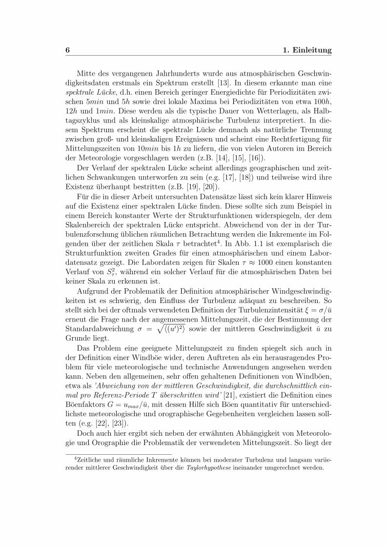
Mitte des vergangenen Jahrhunderts wurde aus atmospharischen Geschwin-digkeitsdaten erstmals ein Spektrum erstellt [13]. In diesem erkannte man einespektrale Lucke, d.h. einen Bereich geringer Energiedichte fur Periodizitaten zwi-schen 5min und 5h sowie drei lokale Maxima bei Periodizitaten von etwa 100h,12h und 1min. Diese werden als die typische Dauer von Wetterlagen, als Halb-tagszyklus und als kleinskalige atmospharische Turbulenz interpretiert. In die-sem Spektrum erscheint die spektrale Lucke demnach als naturliche Trennungzwischen groß- und kleinskaligen Ereignissen und scheint eine Rechtfertigung furMittelungszeiten von 10min bis 1h zu liefern, die von vielen Autoren im Bereichder Meteorologie vorgeschlagen werden (z.B. [14], [15], [16]).

Der Verlauf der spektralen Lucke scheint allerdings geographischen und zeit-lichen Schwankungen unterworfen zu sein (e.g. [17], [18]) und teilweise wird ihreExistenz uberhaupt bestritten (z.B. [19], [20]).

Fur die in dieser Arbeit untersuchten Datensatze lasst sich kein klarer Hinweisauf die Existenz einer spektralen Lucke finden. Diese sollte sich zum Beispiel ineinem Bereich konstanter Werte der Strukturfunktionen widerspiegeln, der demSkalenbereich der spektralen Lucke entspricht. Abweichend von der in der Tur-bulenzforschung ublichen raumlichen Betrachtung werden die Inkremente im Fol-genden uber der zeitlichen Skala τ betrachtet4. In Abb. 1.1 ist exemplarisch dieStrukturfunktion zweiten Grades fur einen atmospharischen und einem Labor-datensatz gezeigt. Die Labordaten zeigen fur Skalen τ ≈ 1000 einen konstantenVerlauf von S2

τ , wahrend ein solcher Verlauf fur die atmospharischen Daten beikeiner Skala zu erkennen ist.

Aufgrund der Problematik der Definition atmospharischer Windgeschwindig-keiten ist es schwierig, den Einfluss der Turbulenz adaquat zu beschreiben. Sostellt sich bei der oftmals verwendeten Definition der Turbulenzintensitat ξ = σ/uerneut die Frage nach der angemessenen Mittelungszeit, die der Bestimmung derStandardabweichung σ =

√〈(u′)2〉 sowie der mittleren Geschwindigkeit u zu

Grunde liegt.

Das Problem eine geeignete Mittelungszeit zu finden spiegelt sich auch inder Definition einer Windboe wider, deren Auftreten als ein herausragendes Pro-blem fur viele meteorologische und technische Anwendungen angesehen werdenkann. Neben den allgemeinen, sehr offen gehaltenen Definitionen von Windboen,etwa als ’Abweichung von der mittleren Geschwindigkeit, die durchschnittlich ein-mal pro Referenz-Periode T uberschritten wird’ [21], existiert die Definition einesBoenfaktors G = umax/u, mit dessen Hilfe sich Boen quantitativ fur unterschied-lichste meteorologische und orographische Gegebenheiten vergleichen lassen soll-ten (e.g. [22], [23]).

Doch auch hier ergibt sich neben der erwahnten Abhangigkeit von Meteorolo-gie und Orographie die Problematik der verwendeten Mittelungszeit. So liegt der

4Zeitliche und raumliche Inkremente konnen bei moderater Turbulenz und langsam variie-render mittlerer Geschwindigkeit uber die Taylorhypothese ineinander umgerechnet werden.


τ

Sτ [a.u.]

101 103 105

10-2

100

2

Abbildung 1.1: Dargestellt ist die Strukturfunktion zweiter Ordnung S2τ fur einen Labor-

(offene Symbole) und einen atmospharischen Datensatz (geschlossene Symbole) in doppelt-logarithmischer Auftragung. In Kapitel 3 werden beide Datensatze (bezeichnet mit Lab undOff) vorgestellt. Im Gegensatz zum atmospharischen Datensatz ist fur den Labordatensatzfur τ > 103 ein klarer Bereich konstanter Strukturfunktionswerte zu erkennen. Fur die atmo-spharischen Daten entspricht der dargestellte Bereich den Skalen von 0.2s bis 105s.

Bestimmung der Maximalgeschwindigkeit umax eine Mittelungszeit ∆t zugrun-de, die mindestens der zeitlichen bzw. raumlichen Integration des verwendetenAnemometers entspricht, oftmals aber auf eine bestimmte Dauer (beispielsweise3s) festgesetzt wird. Zur Bestimmung von u wird uber die Referenzperiode T(zumeist 10min) gemittelt. Der Boenfaktor hangt dabei stark von ∆t bzw. T abund weist allgemein einen hyperbolischen Verlauf uber ∆t/T auf [24].

Eine detailliertere Klassifikation von Windboen findet sich insbesondere imBereich technischer Anwendungen wie der Windenergienutzung. In der Norm IEC61400-1 wird zwischen funf unterschiedlichen Boenarten unterschieden5: Extre-me operating gusts, Extreme direction changes, Extreme coherent gusts, Extremecoherent gusts with direction change und Extreme wind shears. Die Extreme ope-rating gust (EOG) beispielsweise ist definiert durch:

uGust,N = β

(σ

1 + D/10Λ

). (1.7)

Dabei bezeichnet σ die Standardabweichung der Geschwindigkeitskomponentein Hauptwindrichtung, D gibt den Rotordurchmesser (einer Windkraftanlage)an, Λ ist ein Skalenparameter (typischerweise 21m), der Index N bezeichnet dieWiederkehrzeit einer Boe in Jahren und β ist ein Risikoparameter der mit N

5Die Abkurzung IEC steht fur ’International Electrotechnical Commission’.

8 1. Einleitung

ansteigt. Der zeitliche Verlauf der EOG ist ebenfalls definiert und gegeben durch:

u(t) = u0 − 0.37 · uGust,N · sin(

3π

Tt

) [1− cos

(2π

Tt

)]. (1.8)

T bezeichnet die Boendauer und hangt leicht von der Wiederkehrzeit ab, u0 istdie Geschwindigkeit vor und nach Durchgang der Windboe. Die anderen vierDefinitionen sind im Appendix A zusammengefasst. In Abb. 1.2 ist der zeitlicheVerlauf einer EOG Boe wiedergegeben.

t [s]

u(t) [ms-1]

5 15

25

35

T

Abbildung 1.2: Dargestellt ist der zeitliche Boenverlauf nach der Norm IEC 61400-1. DieBoendauer betragt T = 10.5s und die Geschwindigkeit vor und nach Durchgang der Boeu0 = 25ms−1. uGust,N ist mit 14.8ms−1 gegeben.

Ein prinzipieller Schwachpunkt der Charakterisierung von atmospharischerTurbulenz durch die vorgestellten Beschreibungsgroßen (Turbulenzintensitat,Boenfaktor, IEC Definitionen) besteht in der Tatsache, dass hier neben empiri-schen Faktoren nur die Momente erster und zweiter Ordnung in Form von Mittel-wert und Standardabweichung eingehen. Dies ist nur dann ausreichend, wennatmospharische Turbulenz vollstandig durch eine Gauss-Statistik beschreibbarware.

Wie bereits anhand der multifraktalen Eigenschaften turbulenterGeschwindigkeitsfelder verdeutlicht wurde, tritt selbst bei stationarer, ho-mogener und isotroper Turbulenz eine deutlich anomale Statistik der Ge-schwindigkeitsunterschiede zu Tage. Bei instationarer Turbulenz konnen selbstdie Fluktuationen nicht langer als normalverteilt angenommen werden. Einevollstandige Beschreibung allein durch Mittelwert und Standardabweichungist deshalb prinzipiell unmoglich. Aus diesem Grund wird atmospharische


Turbulenz in der vorliegenden Arbeit mit stochastischen Methoden analysiert,die in der Turbulenzforschung etabliert sind und sich nicht auf die erstenbeiden Momente beschranken. Im Mittelpunkt steht dabei die Statistik derGeschwindigkeitsinkremente, die sich als naturliches Maß zur Erfassung undAnalyse von Windboen erweisen [25].

Das zentrale Ziel der Arbeit ist die Charakterisierung der Inkrement- bzw.Boenstatistik unter besonderer Berucksichtigung der Instationaritat des Windes.Zudem wird die Bedeutung der gefundenen anomalen Statistik im Hinblick aufExtremereignisse diskutiert. Diese Thematik wird in den ersten beiden Artikelnbehandelt, die in den Kapiteln 2 und 3 zusammengefasst sind.

In einem weiteren Teil der Arbeit steht die Rekonstruktion turbulenter Zeitrei-hen im Vordergrund, die als Realisationen eines stochastischen Prozesses aufge-fasst werden. Dieser Prozess besitzt neben einem deterministischen einen sto-chastischen Anteil. Der Einfluss des letzteren wird als dynamisches Rauschenbezeichnet. Reale Zeitreihen weisen oftmals einen zusatzlichen Rauschanteil auf,der dem Prozess nachtraglich uberlagert ist und als Messrauschen bezeichnetwird. Die Unterscheidung zwischen beiden Rauscharten ist das zentrale Themades dritten Artikels, der in Kapitel 4 wiedergegeben ist.

Im Folgenden werden die drei im Rahmen dieser Arbeit entstandenen Artikelkurz vorgestellt.

Artikel 1:F. Bottcher, Ch. Renner, H.-P. Waldl and J. Peinke: ’On the statistics of windgusts’, Bound.-Layer Meteor., 108:163-173, 2003.

Wir zeigen, dass die Inkrementstatistik atmospharischer Geschwindig-keiten deutlich intermittenter ist als diejenige stationarer, homoge-ner und isotroper Turbulenz. Wird die auf eine mittlere Geschwin-digkeit bedingte Statistik betrachtet, verschwinden die Unterschie-de weitgehend. In der Wartezeitstatistik von Windboen zeigt sichein Potenzgesetz, das fur Labordaten nicht gefunden wird.

Artikel 2:F. Bottcher, St. Barth and J. Peinke: ’Small and large scale fluctuations in at-mospheric wind speeds’, eingereicht in Stoch. Environ. Res. Risk Assess.

Der Artikel diskutiert die multifraktalen Eigenschaften von unter-schiedlichen atmospharischen Geschwindigkeitszeitreihen und ver-gleicht sie mit Zeitreihen aus Laborexperimenten. Es wird einneues Modell vorgestellt, das die beobachtete Intermittenz als

10 1. Einleitung

Uberlagerung von stationaren Abschnitten homogener und isotro-per Turbulenz erklart. Die Verteilung dieser Abschnitte lasst sichdabei durch eine Weibullverteilung beschreiben.

Artikel 3:F. Bottcher and J. Peinke: ’A generalized method to distinguish between dyna-mical and measurement noise in complex dynamical systems’, zu veroffentlichen.

Wir zeigen, dass sich Messrauschen anhand eines konstanten, zeit-unabhangigen Anteils sowohl beim ersten als auch beim zweitenbedingten Moment offenbart. Die Bedeutung eines solchen Off-sets der Momente fur die Rekonstruktion des deterministischenund stochastischen Anteils der Dynamik wird diskutiert. Fur einenOrnstein-Uhlenbeck Prozess kann der Offset quantitativ hergelei-tet werden, wodurch sich der gesamte Ubergangsbereich von einemreinen Prozess hin zu reinem Rauschen erfassen lasst.

Literaturverzeichnis 11

Literaturverzeichnis

[1] L. F. Richardson. Weather Prediction by Numerical Process. CambridgeUniversity Press, 1922.

[2] A. N. Kolmogorov. The local structure of turbulence in an incompressibleviscous flow for very high Reynolds numbers. Dokl. Acad. Nauk. SSSR,305:301–305, 1941.

[3] A. N. Kolmogorov. A refinement of previous hypotheses concerning the localstructure of turbulence in a viscous incompressible fluid at high Reynoldsnumber. J. Fluid Mech., 13:82–85, 1962.

[4] C. Renner, J. Peinke, and R. Friedrich. Markov properties of small scaleturbulence. J. Fluid Mech., 433:383–409, 2001.

[5] A. N. Kolmogorov. Dissipation of energy in locally isotropic turbulence.Dokl. Akad. Nauk SSSR, 32:16–18, 1941.

[6] G. K. Batchelor. Fluid Dynamics. Cambridge University Press, 1994.

[7] U. Frisch. Turbulence. The legacy of of A. N. Kolmogorov. CambridgeUniversity Press, 1995.

[8] W. D. McComb. The Physics of Fluid Turbulence. Oxford University Press,1996.

[9] S. B. Pope. Turbulent Flows. Cambridge University Press, 2000.

[10] D. J. Tritton. Physical Fluid Dynamics. Oxford University Press, 1998.

[11] E. J. Fordham. The spatial structure of turbulence in the AtmosphericBoundary Layer. Wind Engineering, 90(2):95–133, 1985.

[12] L. F. Richardson. Atmospheric diffusion shown on a distance-neighbourgraph. Proc. R. Soc. London Ser. A, 110:709–722, 1926.

[13] I. van der Hoven. Power spectrum of horizontal wind speed in the frequencyrange from 0.0007 to 900 cycles per hour. J. Meteorol., 14:160–164, 1957.

[14] T. Burton, D. Sharpe, N. Jenkins, and E. Bossanyi. Wind Energy Handbook.John Wiley and Sons, 2001.

[15] J. C. Kaimal and J. J. Finnigan. Atmospheric Boundary Layer Flows. OxfordUniversity Press, 1994.

12 LITERATURVERZEICHNIS

[16] R. B. Stull. An Introduction to Boundary Layer Meteorology. Kluwer Aca-demic Publ., 1994.

[17] U. Hogstrom, J. C. R. Hunt, and A.-S. Smedman. Theory and measurementsfor turbulence spectra and variances in the atmospheric neutral surface layer.Bound.-Layer Meteor., 103:101–124, 2002.

[18] S. Yahaya, J. P. Frangi, and D. C. Richard. Turbulent characteristics of asemiarid atmospheric surface layer from cup anemometers – effects of soiltillage treatment (Northern Spain). Ann. Geophysicae, 21:2119–2131, 2003.

[19] S. Lovejoy, D. Schertzer, and J. D. Stanway. Direct evidence of multifractalatmospheric cascades from planetary scales down to 1 km. Phys. Rev. Lett.,86(22):5200–5203, 2001.

[20] E. W. Schulz and B. G. Sanderson. Stationarity of turbulence in light windsduring the maritime continent thunderstorm experiment. Bound.-Layer Me-teor., 111(3):523–541, 2004.

[21] L. Kristensen, M. Casanova, M. S. Courtney, and I. Troen. In search of agust definition. Bound.-Layer Meteor., 55:91–107, 1991.

[22] J. Wieringa. Gust factors over open water and built-up country. Bound.-Layer Meteor., 3:424–441, 1973.

[23] H. Agustsson and H. Olafsson. Mean gust factors in complex terrain. Me-teorologische Zeitschrift, 13(2):149–155, 2004.

[24] Y. Mitsuta and O. Tsukamoto. Studies on spatial structure of wind gusts.Jour. Applied Meteorol., 281:1155–1160, 1989.

[25] H. Bergstrom. A statistical analysis of gust characteristics. Bound.-LayerMeteor., 39:153–173, 1987.

Chapter 2

On the Statistics of Wind Gusts

In this article a comparative study of velocity measurements inthe free atmosphere and velocity measurements under stationary, lo-cal homogeneous and isotropic conditions is made. The probabil-ity density functions (PDFs) of atmospheric velocity differences aremuch more intermittent than those of stationary, homogeneous andisotropic turbulence1. This directly accounts for an increased prob-ability of observing severe wind gusts. It is shown that atmosphericPDFs become similar to the isotropic ones if they are conditioned onan averaged wind speed value.

Clear differences between isotropic and atmospheric velocity dataare found for the waiting time statistics between successive gustswhich are defined as velocity differences exceeding a given threshold.

2.1 Introduction

The wind in the atmospheric boundary layer is known to be distinctively turbu-lent and instationary. As a consequence the wind speed varies rather randomlyon many different time scales. These time scales range from long-term variations(years) to very short ones (minutes down to less than a second). The latter arecommonly considered to correspond to small-scale (microscale) turbulence. Thesesmall-scale fluctuations are superimposed to the mean velocity varying on diurnalor even larger scales. This distinction between a mean flow and superimposedturbulence is justified by the existence of a spectral gap which means that thereis only little wind speed variation on time scales between about ten minutes andten hours [1].

One of the main challenges in turbulence research is the so-called intermittencyof small-scale turbulence, which corresponds to an unexpected high probability of

1In the following the term ’isotropic turbulence’ instead of ’stationary, homogeneous andisotropic turbulence’ will be used.

14 2. Analysis of Velocity Increments in the Atmosphere

large velocity fluctuations. (Note that there are also other independent definitionsof intermittency related to other phenomena.) For atmospheric winds large ve-locity fluctuations on small scales correspond to gusts. A more precise statisticaldescription of the occurrences of gusts is important for many applications.

The aim of this paper is to find a possible relation between laboratory tur-bulence and the atmospheric small-scale one. The mechanisms ruling the at-mospheric turbulence are quite complex. Roughly the origins of atmosphericturbulence can be divided into friction and thermal effects. The influence ofboth generally depends on many different factors like the thermal stability, thetopography, the geographical position and so on [2].

In laboratory experiments the situation is less complicated and easier to con-trol. Here turbulence may be generated only by flow disturbances, speed anddirection of the mean flow can be kept constant and no buoyancy effects have tobe considered. Despite all these differences between different types of turbulenceit is a common concept [3] that cascade-like processes lead to universal statisticalfeatures of small-scale turbulence.

In this work we analyze two data sets, (a) one from a wake flow behind acylinder recorded in a wind tunnel and (b) data from atmospheric wind.

(a) The velocity of the laboratory data was measured in the plane that isspanned by the cylinder axis and the mean velocity direction at a great distance(100 times the diameter D of the cylinder, D = 0.02m) to the cylinder [4].At these distances the periodical flow patterns (Karman-street) arising directlybeyond the cylinder are vanished and the turbulent wake flow can be consideredto be rather isotropic and fully developed. The Reynolds number is Re = UD

ν≈

30000.(b) The atmospheric data set we use was recorded near the German coast-

line of the North Sea in Emden [5]. The velocity was measured by means of anultrasonic anemometer at 20 m height. The sampling frequency was 4Hz. Themeasuring period took about one year (1997-1998). The distance to the sea is be-tween some kilometers and a few tens of kilometers - depending on the direction.After careful investigation of the quality of the data we examine a representa-tive 275-hour-excerpt of October 1997 and focus on the velocity component indirection of the mean wind [6]. During this period the velocity was recordedcontinuously without significant breaks. It is clear that over such a long periodmeteorological conditions are changing.

In the first part of this paper the statistics of atmospheric wind gusts as asmall-scale turbulence phenomenon are examined using the statistics of the hor-izontal velocity increments. The results are compared to the velocity incrementsof the laboratory data. In the second part we examine the waiting time distri-butions of successive wind gusts to resolve their temporal structure. We findevidence that wind gusts are connected to the instationarity of the wind butcan be reduced to stationary laboratory turbulence if a proper condition on aconstant mean velocity is done.

2.2 Probabilistic Description of Wind Gusts 15

2.2 Probabilistic Description of Wind Gusts

Due to the large size of atmospheric flow dimensions the atmospheric wind isdistinctively turbulent leading to very large Reynolds number Re. Although acharacteristic length scale L for atmospheric turbulent flow structures dependson parameters like the surface roughness z0 or the height z above ground, L maybe of the order of about 100m [2]. With typical wind speeds of U ≈ 10ms−1 andmore Reynolds numbers of Re = UL

ν> 108 are obtained.

Turbulent velocity time series are commonly decomposed into a mean speedvalue u(t) and random fluctuations (turbulence) around it u′(t):

u = u + u′ . (2.1)

In the following only the component in mean wind speed direction is considered.Thus u′ and u denote the fluctuating and the averaged part of the wind speed inmean flow direction.

In wind energy research an averaging period of ten minutes is commonly used,even though the smallest possible averaging period is in general time-dependent[7]. In this paper we are interested in the small-scale fluctuations, thus we onlyneed a lower bound of such an averaging time. The presented analysis was per-formed with different averaging times ranging from one minute up to ten minutes.No significant changes in our results were observed. Thus we proceed with anaveraging period of ten minutes.

The larger the fluctuation values u the more turbulent the wind field becomes.In wind energy research this is often expressed by means of the turbulence in-tensity ξ which is defined as the standard deviation σ in relation to the meanvelocity u [2]:

ξ =σ

u. (2.2)

Nevertheless the value of ξ does not contain any dynamical or time-resolvedinformation about the fluctuation field itself.

To achieve a deeper understanding of wind gusts we investigate how far windgusts are related to the well known features of small-scale turbulence.

As a natural and simple measure of wind gusts we use the statistics of velocityincrements uτ :

uτ = u(t + τ)− u(t) , (2.3)

commonly used for intermittency analysis of small-scale turbulence in laboratorydata [4]. The increments directly measure the velocity difference after a charac-teristic time τ as illustrated in Fig.2.1. So a large increment exceeding a certainthreshold S (uτ > S) can be defined as a gust.

For a statistical analysis we are interested in how frequent a certain incrementvalue occurs and whether this frequency depends on τ . Therefore we first cal-culate the Probability Density Functions (PDFs) p(uτ ) of the increments of the


u [m/s]

3 6

2

6

10

t [s]

uτ

τ

Figure 2.1: The picture shows an arbitrary excerpt of the horizontal wind speed time seriesincluding a strong wind gust.

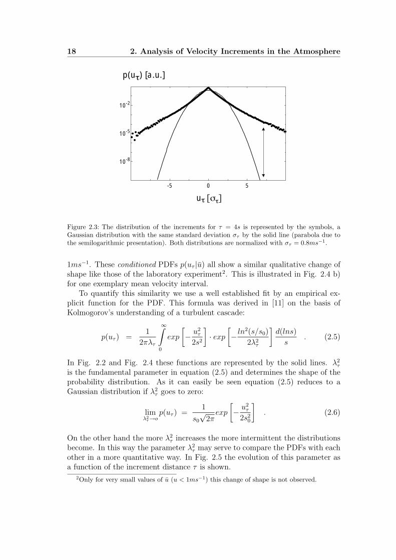
atmospheric velocity fluctuations. In Fig. 2.2 the PDFs for 5 different values ofτ are shown. These distributions are all characterized by marked fat tails anda peak around the mean value. Such PDFs are called intermittent and differextremely from a Gaussian distribution that is commonly considered to be thesuitable distribution for continuous random processes.

A Gaussian or normal distribution is uniquely defined by its mean value µ andits standard deviation σ. Thus every distribution can be compared to a Gaussiandistribution in a quantitative way.

In Fig. 2.3 we compare one of the measured PDFs (τ = 4s) with a normaldistribution with the same σ. In this presentation the different behavior of thetails of both distributions becomes evident. Note that the large increments –located in the tails of the PDFs – correspond to strong gusts. For instance thevalue of uτ = 7σ corresponds to a velocity ascending of 5.6ms−1 during 4s. Asshown in Fig. 2.3 (arrow) the measured probability density of the incrementsof our wind data is about 106 times higher than for a corresponding Gaussiandistribution! The value 106 – for instance – means that a certain gust which isobserved about five times a day should be observed just once in 500 years if thedistribution were a Gaussian instead of the observed intermittent one.

But intermittent distributions seem to appear quite often in natural or eco-nomical systems like in earthquake- [8], foreign exchange market- [9] or even insome traffic-statistics [10].

What kind of statistics do we get in the case of local isotropic and station-ary laboratory experiments? The typical PDFs in laboratory turbulence – asshown in Fig. 2.4 a) – change from intermittent ones for small values of τ to


-10 0 10

10-1

103

uτ [στ]

p(uτ) [a.u.]

Figure 2.2: The PDFs of the increments of the atmospheric velocity fluctuations (normalizedwith στ :=

√u2

τ ) for τ being 0.25s, 1.0s, 6.8s, 32s and 2074s (full symbols from the top to thebottom) are drawn in. They are shifted in vertical direction against each other for a clearerpresentation and the corresponding fits according to Eq. (2.5) are shown as solid curves. p(uτ )is given in arbitrary units (a.u.).

rather Gaussian shaped distributions with increasing τ (τ ≈ T ), where T is thecorrelation or integral time:

T =

∞∫0

R(τ)dτ , (2.4)

well defined for laboratory data where T is found to be about 6 · 10−3s. R(τ)denotes the autocorrelation function of the fluctuations.

For the atmospheric wind data Eq. (2.4) does not converge properly. To fixa large time T we take 1800s as the upper limit of the integral and thus obtainT = 34s.

For the PDFs of the atmospheric velocity field this characteristic change ofshape, even for τ -values higher than T = 34s (as shown in Fig. 2.2) is notobserved.

As already mentioned a fundamental difference between atmospheric and lab-oratory turbulence is that the latter is stationary. In laboratory experimentsone usually deals with fixed speed and direction of the mean wind u, which isobviously never the case for atmospheric wind fields. Therefore in a second stepwe calculate the PDFs of the atmospheric velocity increments only for certainmean velocity intervals. That means that only those increments are taken intoaccount with u ranging in a narrow velocity interval with a width of typically


-5 0 5

10-8

10-5

10-2

p(uτ) [a.u.]

uτ [στ]

Figure 2.3: The distribution of the increments for τ = 4s is represented by the symbols, aGaussian distribution with the same standard deviation στ by the solid line (parabola due tothe semilogarithmic presentation). Both distributions are normalized with στ = 0.8ms−1.

1ms−1. These conditioned PDFs p(uτ |u) all show a similar qualitative change ofshape like those of the laboratory experiment2. This is illustrated in Fig. 2.4 b)for one exemplary mean velocity interval.

To quantify this similarity we use a well established fit by an empirical ex-plicit function for the PDF. This formula was derived in [11] on the basis ofKolmogorov’s understanding of a turbulent cascade:

p(uτ ) =1

2πλτ

∞∫0

exp

[− u2

τ

2s2

]· exp

[− ln2(s/s0)

2λ2τ

]d(lns)

s. (2.5)

In Fig. 2.2 and Fig. 2.4 these functions are represented by the solid lines. λ2τ

is the fundamental parameter in equation (2.5) and determines the shape of theprobability distribution. As it can easily be seen equation (2.5) reduces to aGaussian distribution if λ2

τ goes to zero:

limλ2

τ→op(uτ ) =

1

s0

√2π

exp

[− u2

τ

2s20

]. (2.6)

On the other hand the more λ2τ increases the more intermittent the distributions

become. In this way the parameter λ2τ may serve to compare the PDFs with each

other in a more quantitative way. In Fig. 2.5 the evolution of this parameter asa function of the increment distance τ is shown.

2Only for very small values of u (u < 1ms−1) this change of shape is not observed.


uτ [στ]

p(uτ) [a.u.]

-10 -5 0 5 10

10-4

10-1

102

a)

-5 0 5

10-2

101

104

p(uτ) [a.u.]

uτ [στ]

b)

Figure 2.4: a) The symbols represent the PDFs p(uτ ) of the laboratory increments for differentvalues of τ . From the top to the bottom τ/T takes the values: 0.005, 0.02, 0.17, 0.67 and 1.35.b) The conditioned PDFs of the atmospheric data are presented, here τ/T is 0.008, 0.03, 0.2,0.95 and 1.9. The mean wind interval on which the increments are conditioned covers the valuesbetween 4.5ms−1 and 5.6ms−1. In both cases the solid lines correspond to the fit accordingto Eq. (2.5). PDFs and fits are shifted in vertical direction against each other for clarity ofpresentation.

Other laboratory measurements [11], [12] of λ2τ have shown evidence that it

saturates at approximately 0.2. As shown in Fig. 2.5 λ2τ of the conditioned

wind increments as well as of the laboratory ones is approximately 0.2 for smallτ−values. Furthermore it tends to zero with increasing τ . For the atmosphericdata none of these two features is observed in the case of the unconditionedincrements, λ2

τ is rather independent from τ with a value of about 0.7. A constantbehavior of λ2

τ means that the shape of the PDFs remains unchanged, while itsvariance may change.

Thus we have shown that the anomalous statistics of wind fluctuations on dis-crete time intervals – which are obviously related to wind gusts – can be reducedto the well known intermittent (anomalous) statistics of local isotropic turbu-lence. This result deviates from results of wind data reported in [13], where it isclaimed that their unconditioned wind PDFs behave like those from laboratorymeasurements.


1 10 1000.01

0.1

λ2

τ

Figure 2.5: λ2τ as a function of the increment distance τ is shown for the PDFs of the laboratory

data (open symbols) and of the unconditioned (squares) as well as for the wind data conditionedon the mean velocity interval [4.5; 5.6]ms−1. The axes both are logarithmic. For the laboratorydata τ = 1 corresponds to 10−5s and for the wind data to 0.25s.

2.3 Waiting Time Distribution

So far we have shown how the atmospheric turbulence is related to the laboratoryone in a statistical way. This probabilistic approach describes the frequency withwhich certain gusts occur but it is not clear how they are distributed in time. Inthis sense we now examine the waiting times between successive wind gusts.

The marked fat tail behavior of the unconditioned PDFs – as illustrated inFig. 2.2 – points at an interesting effect. In [14] the equivalence between thedivergence of the moments 〈xq〉 and the hyperbolic (intermittent) form of PDFswhich leads to a power law behavior of the probability distribution is emphasized:

p(x ≥ S) ∝ S−q , S � 1 . (2.7)

A famous example of such a natural power law behavior is the Gutenberg-Richter-law [15] that describes the frequency N of earthquakes with a magnitudebeing greater than a certain threshold M (magnitude):

log(N(m ≥ M)) = a− bM

⇔ N(m ≥ M) ∝ 10−bM . (2.8)

But also the waiting time distribution of fore- and after shocks obey a power-law,what is known as the Omori-law [16].

In this sense we now examine the waiting time distribution of wind gusts.Therefore we refer to the gust illustrated in Fig. 2.1 choosing different thresholds

2.4 Discussion and Summary 21

∆T [s] ∆T [s]10 100 1000

10

100

p(∆T) [a.u.]

~ (∆T)-0.8

10 100 10001

10

100

p(∆T) [a.u.]

~ (∆T)-1.8

a) b)

Figure 2.6: The filled symbols illustrate the waiting time distributions p(∆T ) – given in arbi-trary units – between successive gusts. Additionally two power-law functions are fitted to themeasured values (solid lines).a) The distance is τ/T = 0.3 and the threshold is set to be S = 4.0ms−1. The exponent isfound to be −0.8.b) The distance is τ/T = 2.0 and the threshold is set to be S = 1.5ms−1. The exponent isfound to be −1.8.

S and different increment distances τ (see Eq. (2.3)). Always when the conditionuτ > S is fulfilled a gust event is registered.

The waiting time distributions p(∆T ) for S = 4.0ms−1 and τ = 10s and forS = 1.5ms−1 and τ = 65s are shown in Fig. 2.6 a) and 2.6 b), respectively. Dueto the double-logarithmic presentation both distributions follow a power law butwith different exponents. The exponents depend on S and τ . This power lawbehavior of the waiting time distributions is only observed for the atmosphericwind data and not for the stationary laboratory one.

2.4 Discussion and Summary

On the basis of well defined velocity increments an analogous analysis of mea-sured wind data and measured data from a turbulent wake was performed. Thestatistics of velocity increments, as related to the occurrence frequency of windgusts, showed that they are highly intermittent. These anomalous (not Gaus-sian distributed) statistics explain an increased high probability of finding stronggusts. This could be set in analogy with turbulence measurements of an ideal-ized, local isotropic laboratory flow if a proper condition on a mean wind speedwas performed. This result is rather astonishing, insofar as solely the conditionon the mean velocity leads to a good agreement between the PDFs of the windvelocity increments and those of the laboratory wake flow. At least for our data


it seems to be not necessary to introduce further conditions which take specialmeteorological situations into account. A possible explanation is the proposeduniversality of small-scale turbulence which means that the statistics of the small-scale fluctuations become independent of the driving large scale structures.

As a further statistical feature of wind gusts we have investigated the waitingtimes between successive gusts exceeding a certain strength. Here we find power-law-statistics (fractal statistics) – similar to earthquake statistics – that can notbe reproduced in laboratory measurements.

To conclude we have shown two important aspects of wind gusts. The overalloccurrence statistics could be set into analogy to the anomalous statistics ofvelocity increments in local isotropic turbulence. The time structure of successivegust events displays fractal behavior. We think that these results may be helpfulfor a better characterization and understanding of gust events.

Of course we have to note that these results are obtained from one singlewind data set. It should be very interesting to explore not only the effect ofconditioning on a mean wind velocity but also on different flow situations ordifferent boundary layer or other environmental conditions.

Bibliography 23

Bibliography

[1] E. Hau. Windturbines: Fundamentals, Technologies, Application, and Eco-nomics. Springer, 2000.



[4] St. Luck. Skalenaufgeloste Experimente und statistische Analysen von tur-bulenten Nachlaufstromungen. PhD thesis, Carl-von-Ossietzky University ofOldenburg, 26111 Oldenburg, Germany, 2000.

[5] H. Hohlen and J. Liersch. Synchrone Messkampagnen von Wind- und Wind-kraftanlagendaten am Standort FH Ostfriesland, Emden. DEWI Magazin,12:66–74, 1998.

[6] F. Bottcher, C. Renner, H.-P. Waldl, and J. Peinke. Problematik derWindboen. DEWI Magazin, 2001.

[7] G. Trevino and E. L. Andreas. Averaging intervals for spectral analysis ofnonstationary turbulence. Bound.-Layer Meteor., 95(2):231–247, 2000.

[8] D. Schertzer and S. Lovejoy. Multifractal generation of Self-Oranized Criti-cality. Fractals Nat. Appl. Sci., A-41:325–339, 1994.

[9] S. Ghashghaie, W. Breymann, J. Peinke, P. Talkner, and Y. Dodge. Turbu-lent cascades in foreign exchange markets. Nature, 381:767–770, 1996.

[10] J. C. Vassilicos. Turbulence and Intermittency. Nature, 374:408–409, 1995.

[11] B. Castaing, Y. Gagne, and E. J. Hopfinger. Velocity probability densityfunctions of high Reynolds number turbulence. Physica D, 46(2):177–200,1990.

[12] B. Chabaud, A. Naert, J. Peinke, F. Chilla, B.Castaing, and B. Hebral.Transition toward developed turbulence. Phys. Rev. Lett., 73(24):3227–3230,1994.

[13] M. Ragwitz and H. Kantz. Indispensable finite time corrections for Fokker-Planck equations from time series data. Phys. Rev. Lett., 87(25):254501,2001.

24 BIBLIOGRAPHY

[14] D. Schertzer and S. Lovejoy. Nonlinear Variability in Geophysics 3. LectureNotes, Cargese, 1993.

[15] B. Gutenberg and C. F. Richter. Eathquake magnitude, intensity, energyand acceleration. Bull. Seismol. Soc. Am., 46:105–143, 1956.

[16] F. Omori. On the aftershocks of earthquakes. J. Coll. Sci. Imp. Univ. Tokyo,72:111, 1894.

Chapter 3

Small and Large ScaleFluctuations in AtmosphericWind Speeds

In this article atmospheric wind speeds and their fluctuations atdifferent locations (onshore and offshore) are examined. One of themost striking features is the marked intermittency of probability den-sity functions (PDF) of velocity differences – no matter what locationis considered. The shape of these PDFs is found to be robust over awide range of scales which seems to contradict the mathematical con-cept of stability where a Gaussian distribution should be the limitingone.

Motivated by the instationarity of atmospheric winds it is shownthat the intermittent distributions can be understood as a superpo-sition of different subsets of stationary, homogeneous and isotropicturbulence. Thus we suggest a simple stochastic model to reproducethe measured statistics of wind speed fluctuations.

3.1 Introduction

Atmospheric wind may be seen as a prime example of a turbulent velocity fieldwith very high Reynolds numbers of about Re ≈ 108 [1]. Reynolds numbersas large as this prevent analytical calculations and direct numerical simulations.Therefore the flow has to be described in a statistical way. For the estimation ofextreme loads as well as for risk estimations the statistics of velocity fluctuationsu′(t) and velocity differences should be known1. It has been shown that these

1In the following we only consider the wind speed components in mean wind speed directioninstead of the vectorial velocity.

26 3. Superposition Modell for Atmospheric Wind Speeds

statistics obey non-Gaussian, intermittent distributions (e.g. [2], [3]) that directlycorrespond to an increased number of wind gusts [4].

Nevertheless, for most technical and meteorological problems fluctuations aswell as fluctuation differences are assumed to obey Gaussian statistics. Thereforesimulations of atmospheric velocities are often based on Gaussian processes [5].

Fluctuation differences are commonly measured using velocity increments:

uτ (t) := u(t + τ)− u(t) . (3.1)

Large increment values can be identified as wind gusts as long as the time step τis rather small. The demand for a small τ -value (typically less than a minute) isdue to the fact that gusts are related to large velocity rises during short times.Rises that occur over time steps of several hours – for instance – are not calledwind gusts but large scale variations.

The difficulty to fix a suitable time scale mirrors the fact that atmosphericwinds exhibit variations on any time scale – in principle ranging from seconds(and less) up to centuries. For most practical applications, such as engineeringand meteorology one mainly distinguishes between large scale variations such asdiurnal, weekly and seasonal changes and variations on small scales often referredto as atmospheric turbulence or gustiness [1]. The existence of a mesoscale gapas proposed by [6] which divides small (micro) and large (macro) scales in amore rigorous way has strongly been debated in recent years (e.g. [7], [8]).

In this paper we focus on the scale dependent statistics of atmospheric incrementsand compare them to that of homogeneous, isotropic and stationary turbulence2

as realized in laboratory experiments. For isotropic turbulence the statisticalmoments of increments, the so-called structure functions have been intensivelystudied [9]. Their functional dependence on the scale τ is described by a varietyof multifractal models. Besides the analysis of moments, probability densityfunctions (PDFs) are often considered. These show a transition from Gaussiandistributions to intermittent (heavy-tailed) ones as scale decreases. Unfortunatelythe analysis of moments as well as that of probability density functions p(uτ ) ismore or less restricted to the inertial range – the range of scales larger than theTaylor scale Θ (where dissipation effects become significant) and smaller thanthe integral scale3 T .

The challenge is to describe and to explain the measured fat-tailed distri-butions and the corresponding non-convergence to Gaussian statistics. Largeincrement values in the tails directly correspond to an increased probability4

2In the following the term ’isotropic turbulence’ instead of ’homogeneous, isotropic andstationary turbulence’ will be used.

3Normally Θ and T denote length scales. For constant mean velocities and applying Taylor’shypothesis of frozen turbulence length- can be defined as time-scales as well. Here we willproceed with corresponding time scales.

4The probability to observe an increment uτ ε [uτ , uτ + duτ ] is just given by p(uτ )duτ .

3.2 The Data 27

(risk) to observe large and very large events (gusts). As pointed out in [10] theprobability to observe large events – e.g. events twice as large as a reference –can become negligible for a Gaussian while for heavy-tailed distributions there isstill a significant probability to observe it.

The atmospheric PDFs – we examine here – differ from those of turbulentlaboratory flows where – with decreasing scale – a change of shape of the PDFs isobserved (e.g. [11]). For large scales the distributions are Gaussian while for smallscales they are found to be intermittent. The atmospheric PDFs however changetheir shape only for the smallest and then stay intermittent for a broad rangeof scales. Such a constant shape for larger and larger scales is expected only forstable distributions such as Gaussian ones or the Levy stable laws [12]. Althoughthe decay of the tails indicates that distributions should approach Gaussian ones(as for isotropic turbulence) they show a rather robust exponential-like decay.This point will be clarified in chapter 3.3.2.

In chapter 3.3.1 and 3.3.2 it will be shown that atmospheric increments behavequite similar to those of isotropic turbulence for small scales but differ significantlyfor large ones. We therefore introduce a model – chapter 3.4 – that interpretsatmospheric increment statistics as a large scale mixture of subsets of isotropicstatistics. When mixing is weak the same statistics as for isotropic turbulence arerecovered while for strong mixing robust intermittency is obtained. In chapter3.5 the results are briefly discussed.

3.2 The Data

The analysis presented in the following is based on one laboratory and four dif-ferent atmospheric data sets. In addition to accessibility reasons the latter werechosen in such a way that their environmental and meteorological characteris-tics differ significantly. Therefore one offshore and three onshore data sets areexamined. Additionally a laboratory data set was chosen as an example of anapproximately isotropic turbulent wake-flow.

The first data set was recorded in October 1997 near the German coastline ofthe North Sea in Emden at a height of 20m by means of an ultrasonic anemometer[13]. The wind speed was measured continuously over a period of 275 hours. Inthe following this data set will be referred to as On1.

The second data set – denoted as On2 – was obtained from a hot-wire mea-surement 6m above the ground (in flat terrain) [14]. Here the wind speeds ofapproximately one hour were considered.

On3 – the third data set was recorded in a very complex terrain near Oberzeir-ing (1900m above the sea level) in Austria in 2001 [15]. The velocity was measuredby means of an ultrasonic anemometer. The data consists of 255 non-successiveblocks of 4 hours length. The choice was made in order to obtain complete andcontinuous data within each block.


The fourth data set – referred to as Off – was recorded during an offshoremeasuring campaign at Roedsand in the Danish Baltic Sea at 30m height between1998 and 1999 [2]. From this period 58 non-successive days were chosen. Againthe choice was made in order to obtain complete and continuous data for eachday.

The laboratory data – denoted as Lab – were obtained from a wake flowmeasurement in the wind tunnel of Erlangen in 1998 [16]. A hot-wire was located2m behind a cylinder of diameter D = 0.02m in the plane spanned by the cylinderaxis and the mean velocity direction. Here the turbulent flow can be consideredto be locally isotropic and fully developed. With a mean velocity of u = 20.9ms−1

a Reynolds number of Re = uDν−1 ≈ 30, 000 is obtained. Taylor and integralscale are found to be Θ ≈ 2 · 10−4s and T ≈ 6 · 10−3s, respectively.For atmospheric data sets it is difficult to define an integral scale T because of theinstationarity of atmospheric velocities that causes very long-range correlationsR(τ) ∝ 〈u(t + τ)u(t)〉 so that the integral time

T :=

∞∫0

R(τ) dτ (3.2)

cannot be estimated properly. Only for On2 an estimate of the integral timecan be given because of the rather constant flow conditions during the shortmeasuring period of about 1 hour.

For On2 the Taylor scale Θ can be calculated while for all other atmosphericdata sets the sampling frequency is too low for Θ to be resolved.In Table 3.1 a short overview of the most important specifications of all five datasets is given.

On1 On2 On3 Off Lab

N [1] 3,958,874 20,480,000 14,688,000 25,056,000 12,500,000blocks [1] 1 1 255 58 100f [Hz] 4 5,000 4 5 100,000u [ms−1] 3.4 8.3 6.6 9.6 20.9min [ms−1] 0.0 0.8 0.02 0.6 15.9max [ms−1] 18.1 18.1 39.0 36.1 25.5σ [ms−1] 1.7 2.3 4.2 3.2 1.1Θ [s] < 0.25 ≈ 0.01 < 0.25 < 0.2 ≈ 2 · 10−4

T [s] – ≈ 14 – – ≈ 6 · 10−3

Table 3.1: The table summarizes some characteristic values of the different data sets, from topto bottom these are number of data points N , number of blocks, sample frequency f , meanvelocity u, minimum, maximum, average standard deviation σ, Taylor scale Θ and integralscale T .

3.3 Analysis 29

3.3 Analysis

3.3.1 Scaling in Isotropic and Atmospheric Turbulence

The central assumption for turbulent velocity time series is that they have a self-similar structure (a direct consequence of scale invariance of the Navier StokesEquation) in the inertial range. This means that within this range the disorderof velocity fluctuations has a similar structure on every scale but with a scale-dependent magnitude. To quantify this one usually calculates the (absolute)moments of increments

Snτ = 〈|uτ |n〉 , (3.3)

which are also called structure functions of order n. Instead of calculating theabsolute moments one can also consider 〈un

τ 〉 (see [17] for a more detailed discus-sion).

In isotropic turbulence structure functions are assumed to scale as:

Snτ ∝ τ ζn . (3.4)

A linear (monofractal) scaling exponent ζn corresponds to a self-similar structureas proposed by Kolmogorov in 1941 [18] who found that the scaling exponentshould be

ζn =n

3(3.5)

due to dimensional reasons. Instead of this linear behavior various experimentssuggest that the scaling exponent is a non-linear function of n. In 1962 Kol-mogorov [19] introduced the following non-linear (multifractal) exponent

ζn =n

3+

µ

18(3n− n2) (3.6)

motivated by the model of a turbulent cascade with a lognormally distributedenergy transfer rate. The parameter µ is called intermittency correction and isfound to be close to 0.25 [20] which corresponds to ζ6 = n

3− µ = 1.75. This is in

agreement with the examined data sets where ζ6 takes values between 1.67 and1.80 as shown in Fig. 3.1 a).In [21] another formula was proposed which seems to fit experimental data slightlymore accurately than Eq. (3.6):

ζn =n

9+ 2− 2

(2

3

)n/3

. (3.7)

There are other models besides these two multifractal ones, e.g. [7], [22]. Thedifferences in ζn in all these models are rather small (at least for small orders)


2 4 6 80

1

2

ζn

n

LabOn1On2

OffOn3

a)

0.1 1

0.01

1

100 b)

S3τ

Snτ

Figure 3.1: a) This plot shows the scaling exponents ζn as a function of order n for all fivedata sets. Additionally the linear scaling law given by Eq. (3.5) (straight line) and the non-linear laws according to Eq. (3.6) (curved line) and Eq. (3.7) (curved dashed line) are shown.b) The structure functions of order 2, 4 and 6 are plotted against that of order 3 in a double-logarithmic presentation (vertically shifted for clarity of presentation). The open symbolsbelong to On1, the filled ones to Lab.

so for simplicity we will restrict following discussions to the models given by Eq.(3.6) and Eq. (3.7).

To estimate the dependence of ζn on n one has to calculate ζn first. The mostcommon way to do this is to plot log(Sn

τ ) against log(S3τ ) – a method referred to

as Extended Self Similarity (ESS) [23]. The slope of the resulting line is equalto ζn. This is shown in Fig. 3.1 b) exemplary for data sets On1 and Lab. Inboth cases the slopes are in quite good agreement with Eq. (3.6) and Eq. (3.7).The slopes of On1 show small deviations from linear behavior for large values.These correspond to large scales τ that might not belong to the inertial rangeanymore. This already indicates that care should be taken when transferringstandard analysis of isotropic to atmospheric turbulence.The difference between isotropic and atmospheric turbulence statistics becomemore obvious when calculating the flatness F . Assuming inertial range scalingaccording to Eq. (3.3) and (3.4) the flatness should scale as well and is given by:

F :=〈u4

τ 〉〈u2

τ 〉2 ∝ τ ζ4−2ζ2 . (3.8)

If Eq. (3.6) is a suitable description5 the flatness scales according to:

F ∝ τ−4µ/9 , (3.9)

5Eq. (3.7) and other multifractal models yield very similar results because such low-orderexponents as ζ4 and ζ2 are quite indistinguishable from each other.

3.3 Analysis 31

τ [a.u.]

F

101 1032

5

10 On1Lab

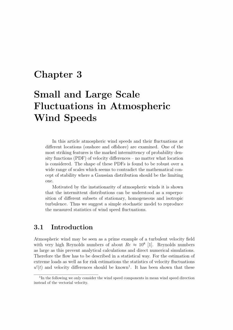
Figure 3.2: The open symbols show the flatness F of On1 as a function of scale with τ = 0.25s.The filled symbols represent the flatness of Lab with τ = 0.002T ≈ 10−5s. Additionally fitsaccording to Eq. (3.9) (straight lines) are drawn in with µ = 0.29 (On1) and µ = 0.26 (Lab).The horizontal dashed line marks F = 3 (as for a Gaussian distribution).

as is easily shown inserting Eq. (3.6) into Eq. (3.8). As shown in Fig. 3.2the measured flatness of the data shows this scaling behavior but the absolutevalues of F are very different for different data sets. While for the Lab data setflatness approaches F ≈ 3 for large τ it saturates at F ≈ 6 for the On1 data set.The flatness of On3 and Off saturates at F ≈ 5 while for On2 it goes down to 3.5.

Calculating the flatness of a variable x is often done to estimate the shape of thePDF p(x). A Gaussian distribution has flatness 3. Deviations from this valuecan be taken as a hint for a non-Gaussian shape of PDFs. In the following theincrement PDFs of the given data sets will be examined.

3.3.2 Probability Density Functions in Turbulence

Alternatively to the analysis of scaling exponents one can directly investigate thePDFs of velocity increments p(uτ ). The scaling behavior as well as all moments(including derived quantities such as flatness or skewness) are immediately givenif the distributions on every scale are known.

In principle the knowledge of all moments Snτ and the knowledge of the PDFs

should contain the same information as can be seen by means of the characteristicfunction ϕ(k) – which is the Fourier transform of the PDF – defined as:

ϕ(k) :=∞∑

n=1

Snτ

(ik)n

n!. (3.10)


Nevertheless the relation between moments and PDFs is not unique. In [12] it ispointed out that two different PDFs can have exactly the same moments.

From many experiments of isotropic turbulence it is well known that theshape of a PDF changes with scale. Going from larger to smaller scales thedistributions become more and more heavy-tailed while for τ ≥ T a Gaussiandistribution is obtained. This scale-dependent shape corresponds to non-linearscaling exponents – as introduced in Eq. (3.6) and Eq. (3.7) – while a linearbehavior Sn

τ = anταn = anβ

n according to Eq. (3.5) leads to a constant shape.This can be seen by means of the characteristic function in Eq. (3.10) that staysthe same for a linear exponent only k is rescaled according to k = βk.

The analysis of scaling exponents thus focusses on the change in shape of dis-tributions while the shape itself is of minor interest and could even be determinedwrongly as shown at the end of the last chapter. Therefore we will henceforthfocus on the analysis of PDFs.

-5 0 5

10-3

101

-5 0 5

10-3

101

a) b)

p(uτ) [a.u.]

uτ / στ uτ / στ

p(uτ) [a.u.]

Figure 3.3: a) Symbols represent normalized PDFs (with their scale-dependent standarddeviation στ =

√〈u2

τ 〉) of the Lab data set. From top to bottom τ takes the val-ues: 0.01T , 0.05T , 0.2T and 1.0T where T ≈ 0.006s denotes the integral time.b) Symbols represent normalized PDFs of the atmospheric data set On1 with τ = 0.5s, 2.5s,25s, 250s and 4000s. All graphs – in a) and b) – are plotted in a semi-logarithmic presentationand are shifted against each other in vertical direction for clarity of presentation. The solidlines correspond to a fit of the distributions according to Eq. (3.11).

In accordance with Eq. (3.6) (that was derived from the assumption of a log-normally distributed energy transfer rate) B. Castaing et al. [11] introduced amodel in which the increment distribution p(uτ ) is interpreted as a superpositionof Gaussian ones p(uτ |σ) with standard deviation σ. The standard deviationitself is distributed according to a lognormal distribution f(σ). The increment

3.3 Analysis 33

distribution thus reads

p(uτ ) =

∞∫0

dσ p(uτ |σ) · f(σ)

=

∞∫0

dσ1

σ√

2πexp

[− u2

τ

2σ2

]· 1

σλ√

2πexp

[− ln2(σ/σ0)

2λ2

](3.11)

and will henceforth be referred to as the Castaing distribution. (It is also possibleto take distributions different to the log-normal one – see Appendix B.)

Two parameters enter this formula, namely σ0 and λ2. The first is the me-dian of the lognormal distribution, the second its variance. The latter determinesthe form (shape) of the resulting distribution p(uτ ) and is therefore called formparameter. On one side the larger λ2 becomes the broader the lognormal dis-tribution and the broader the range of σ that contributes to the integral in Eq.(3.11). On the other side the range of σ becomes smaller and smaller with de-creasing form parameter. In the limit of vanishing λ the lognormal becomes adelta distribution

limλ→0

(1

σλ√

2πexp

[− ln2(σ/σ0)

2λ2

])= δ(σ − σ0) , (3.12)

so that p(uτ ) is reduced to a Gaussian distribution with variance σ20.

With a proper choice of the form parameter the PDFs p(uτ ) can well be fittedas it is shown in Fig. 3.3 a) and Fig. 3.3 b). In Fig. 3.3 a) – where the Lab dataset is presented – the expected change of shape from intermittent to Gaussiandistributions with increasing scale is clearly seen.In contrast to this behavior the PDFs of On1 in Fig. 3.3 b) look totally different.They are much more intermittent and do not approach a Gaussian distributioneven for very large scales. For scales larger than about 25s the shape remainsrather constant. This is in accordance with the finding of the slow decrease offlatness shown in Fig. 3.2 because in the lognormal model flatness is linked tothe form parameter [24] according to

λ2 ∝ ln

(F

3

). (3.13)

In this sense constant flatness larger than 3 corresponds to constant λ2 largerthan 0 and thus to rather scale-independent intermittent distributions as shownin Fig. 3.3 b) exemplary for the On1 data set. The λ2-values for all data sets areillustrated in Fig. 3.4 revealing a weak scale-dependence for On1, On3 and Offand a large one for On2 and Lab.

In isotropic turbulence scale-independent distributions are also found whenthe scales are larger than the integral time T . In this case the distributions


10 10000.001

0.01

0.1

τ

λ2

On1

Off

On2Lab

On3

Figure 3.4: The form parameter for the data sets On3, On1, Off, On2 and Lab are shown indouble-logarithmic presentation. In that order τ = 1 corresponds to 0.25s, 1s, 1s, 0.02s and10−5s (0.002T ). The solid line represents a fit according to Eq. (3.23).

are always Gaussian [25]. Such stable Gaussian PDFs can be seen as the resultof a stochastic Gaussian process. The other class of stable distributions are theso-called Levy distributions – characterized by power-law tails – which can be ob-tained from a fractional stochastic process. The observed atmospheric incrementPDFs show robust (stretched) exponential tails that decay faster than a power-law and slower than a Gaussian distribution. So the question arises whether theatmospheric PDFs can be explained as a fractional process or as a superpositionof different Gaussian processes in analogy to the Castaing distribution. To de-cide this the concept of stability and the connection to increment analysis shouldbriefly be introduced.

3.3.3 Stable Distributions

Consider the sum sm =m∑i

xi of m independent and identical distributed (i.i.d.)

variables. The distribution of the variable x is denoted with p and that of thesum-variable by p. The distribution p (or p respectively) is then called stable iffor large m (m →∞)

p(x′) dx′ = p(x) dx with x′ = Ax + B (3.14)

is fulfilled [12]. This means that for sufficiently large m the shape of the distri-bution does not change as m increases.

3.3 Analysis 35

Transferred to increment analysis an increment over a scale τ can be identifiedas variable x and the increment of a larger scale mτ as the sum-variable sm. Itis immediately shown that

umτ (t) =m−1∑i=0

uτ (t + iτ) , (3.15)

which means that a large increment can be expressed as the sum of smaller ones.When the PDFs of large and small increments are the same this indicates a stablePDF.

The most famous stable distribution is the Gaussian one. Beside this P. Levy[26] showed that there exists a whole class of stable distributions. Restricting tosymmetric distributions their characteristic functions read:

ϕ(k) = exp [iγk − c|k|α] ; 0 < α ≤ 2. (3.16)

For asymmetric distributions the characteristic function becomes more compli-cated (e.g. [27]). The analytical form of the corresponding PDFs is only knownfor some special cases (e.g. for α = 1 it is the Cauchy distribution) but theirasymptotic behavior is always known and given by:

p(x) ∝ C |x|−(1+α) ; x � 1 . (3.17)

This algebraic decay of tails means that all higher order moments larger thanorder α do not exist. Generally, distributions with tails decaying faster than∝ |x|−3 (defined variance) can only converge to a Gaussian while slower decayingtails indicate that they can only converge to a Levy stable law.

As already mentioned the examined atmospheric PDFs show a faster thanalgebraic decay (compare Fig. 3.3 b) and Fig. 3.8 a), b), c), d)) so it is ex-pected that they converge to Gaussian statistics for large scales. Therefore theobserved robust intermittency should be explained by mixing different Gaussiandistributions rather than by a fractional stochastic process.


3.4 Superposition Model for Atmospheric Tur-

bulence

In [4] it was proposed to take the instationarity of long atmospheric time seriesinto account. In this sense the observed intermittent form of PDFs for all exam-ined scales are found to be the result of mixing statistics belonging to differentflow situations. These are characterized by different mean velocities as schemat-ically illustrated in Fig. 3.5. When the analysis by means of increment statisticsis conditioned on periods with constant mean velocities results are found to bevery similar to those of isotropic turbulence. This can be set in analogy to theCastaing distribution that interprets intermittent PDFs as a superposition of in-tervals with different standard deviations.

u [a.u.]

t [a.u.]

u

Figure 3.5: Illustration of different mean velocity intervals. Within these intervals statisticsshould be the same as for isotropic turbulence. The magnitude of variations (standard devia-tion) grows with mean velocity according to Eq. (3.24).

Thus we propose a model that describes the robust intermittent atmosphericPDFs as a superposition of those of isotropic turbulent subsets that are denotedwith p(uτ |u) and given by Eq. (3.11). Knowing the distribution of the meanvelocity h(u) the PDFs become:

p(uτ ) =

∞∫0

du h(u) · p(uτ |u) . (3.18)

To find a suitable averaging time defining the mean value u is a non-trivial prob-lem due to the lack of a distinct mesoscale gap and is not the concern of thepresent paper (see e.g. [28]). As a first approximation we fix the averaging time

3.4 Superposition Model for Atmospheric Turbulence 37

0 5 10 15

0.1

0.3

0.5

h(u)

u [m/s]

On1

On2

Off

On3

Figure 3.6: Symbols represent measured mean velocity distributions (averaged over 10 min) ofthe four atmospheric data sets On1, On2, On3 and Off. Solid lines are fits according to Eq.(3.19). The parameters are: k = 2.0, 7.8, 1.8, 3.3 and A = 2.9, 4.8, 7.1, 8.7 for On1, On2,On3 and Off respectively.

to be 10 minutes. In [4] it is shown that with this choice a partition into isotropicsequences is achieved. Furthermore we assume h(u) to be a Weibull distribution

h(u) =k

Ak· uk−1 · exp

[−

( u

A

)k]

, (3.19)

that contains two parameters A and k. Both assumptions are well established inmeteorology [1]. In Fig. 3.6 it is shown that the Weibull distribution h(u) is agood representation of the measured distributions of mean velocities.

Inserting Eq. (3.19) and Eq. (3.11) into Eq. (3.18) the following expressionfor atmospheric PDFs is obtained:

p(uτ ) =k

2πAk

∞∫0

du

∞∫0

dσ uk−1 exp

[−

( u

A

)k]

× 1

λσ2exp

[− u2

τ

2σ2

]exp

[− ln2(σ/σ0)

2λ2

]. (3.20)

Next we briefly discuss the meaning of the two parameters A and k. They playa similar role as σ0 and λ2 in the Castaing distribution. Parameter A is closelyrelated to the expectation value (〈u〉 = A · Γ(1 + k−1)) of the mean velocity. Pa-rameter k determines the shape of the distribution. Small values of k correspondto a broad distribution h(u) so that many different mean velocities contribute


σ0 [m/s]

2 4 6 8

1

2

u [m/s]

Figure 3.7: Standard deviation σ0 as a function of u for τ = 1s and τ = 50s.

significantly to the integral in Eq. (3.20). Large k-values however prevent thiscontribution and h(u) is closely centered around A. In the limit of very large ka delta distribution is obtained:

limk→∞

(k

Akuk−1 exp

[−

( u

A

)k])

= δ(u− A) . (3.21)

So for very large k-values Eq. (3.20) converges to Eq. (3.11) i.e. to isotropicturbulence. For additionally large τ and accordingly vanishing λ2 one finally gets

limk→∞

limτ→∞

p(uτ ) =1

σ0

√2π

exp

[− u2

τ

2σ20

](3.22)

which is a pure Gaussian density with variance σ20(A). For small k-values the

distributions remain intermittent even for large scales. Here intermittency iscaused by the mixing of periods of different mean velocities.

To apply Eq. (3.20) to experimental data one has to know the parameters A, k,σ0 and λ2. Parameters A and k can directly be estimated from data by fitting aWeibull distribution given in Eq. (3.19) to the measured distribution of u. Thisis illustrated in Fig. 3.6 for all examined atmospheric data sets.

Next λ2 = λ2(τ, u) and σ0 = σ0(τ, u) have to be known. From isotropicturbulence it is well-established that the form parameter decreases monotonouslyin scale. Scaling of flatness according to Eq. (3.8) together with Eq. (3.13)directly leads to a logarithmic dependence of λ2 on τ :

λ2 = au − bu · ln(τ) . (3.23)

3.4 Superposition Model for Atmospheric Turbulence 39

To confirm this in Fig. 3.4 the form parameter of the Lab data set is fitted withEq. (3.23). For a deeper discussion on the scale dependence of λ2 see [29].

The dependence of λ2 on u is small (e.g. [11] found a slower decay of λ2 forincreasing Reynolds numbers Re ∝ u). As a first approximation we will disregardit.

The parameter σ0 – the most probable standard deviation – generally growswith scale and mean velocity. The scale dependence drops out automaticallywhen considering normalized PDFs as it is done here. For the u-dependence weassume a linear relation

s0 = bτ · u , (3.24)

which is supported from the measured standard deviation σ0, shown in Fig. 3.7.Thus, to apply Eq. (3.20) we need to calculate A and k from measured mean

velocity distributions. Additionally we consider a logarithmic dependence of λ2

on τ and a linear one for σ0 on u. Given that we are interested in a preferablysimple reconstruction of PDFs by means of Eq. (3.20) we will disregard themore complex parameter relations here.

With these parameters atmospheric increment PDFs can be determined well fromEq. (3.20). As shown in Fig. 3.6 for On1, On 3 and Off rather small k-valuesof 2.0 1.8 and 3.3 are obtained indicating that resulting PDFs are heavy-tailedalso for large scales. In Fig. 3.8 a) and 3.8 b) and Fig. 3.8 d) the correspondingPDFs as well as fits according to Eq. (3.20) are presented. The fits agree quitewell with measured distributions. For all three data sets the tails show a similardecay for large scales and are close to a straight line which corresponds to anexponential decay due to the semi-logarithmic presentation.

In contrast to this behavior the PDFs of On2 and the fits according to Eq.(3.20) – shown in Fig. 3.8 c) – approach a Gaussian distribution for large scaleswhich is in accordance with the large k-value of 8.7 as it is found in Fig. 3.6.This large k-value mirrors the fact that On2 was measured just over a shortperiod of time (approximately 1 hour) with rather constant flow conditions. Thismeans that as the flow becomes more and more stationary the superposition ofdifferent mean velocities becomes weaker and weaker. In the limit of a stationaryvelocity – as realized for Lab and approximately forOn2 – isotropic turbulence isrecovered and large scale intermittency disappears.

Note, the intention of using Eq. (3.20) is not to get the best possible fits ofthe measured PDFs but to model PDFs at specific locations (with a specificmean velocity distribution) a priori. The measured PDFs could also be fittedby stretched exponential distributions [12] or by Eq. (3.11) as it is done inFig. 3.3 b) for instance. These fits are based on a posteriori measurementshowever. Neither scaling models nor Eq. (3.11) are able to explain a flatness


larger than 3 and correspondingly intermittent PDFs for large scales outside ofthe inertial range as it is done by Eq. (3.20). This has interesting consequencesfor atmospheric velocities. For isotropic turbulence statistical properties of theflow can well be modelled. Thus knowing the composition of isotropic subsets itshould be possible to model atmospheric velocity statistics as well.

-10 0 10

10-10

10-6

10-2

p(uτ) [a.u.]

uτ / στ

-10 0 10

10-10

10-6

10-2

p(uτ) [a.u.]

uτ / στ

a)

c)

-10 0 10

10-8

10-4

-10 0 10

10-7

10-3

p(uτ) [a.u.]

uτ / στp(uτ) [a.u.]

uτ / στ

b)

d)

Figure 3.8: The symbols represent the normalized PDFs of the four atmospheric datasets in semi-logarithmic presentation. Solid lines correspond to a fit of distribu-tions according to Eq. (3.20). All graphs are vertically shifted against eachother for clarity of presentation. From top tobottom τ takes the following values:a) Off: 0.2s, 10s, 20s, 200s and 2000s. b) On1: 0.5s, 2.5s, 25s, 250s and 4000s. c) On2:2ms, 20ms, 200ms and 2000ms. d) On3: 0.25s, 2.5s, 25s and 250s.

3.5 Conclusions 41

3.5 Conclusions

The presented analysis provides a good way to estimate and to explain robust andmarkedly intermittent PDFs of atmospheric increments. As desired the methodrecovers results of isotropic turbulence but is also able to take the large scalevariations into account properly. A rigorous separation of time scales – which isvery difficult – is not necessary for our model.

Standard analysis applied to isotropic turbulence cannot be transferred tolong atmospheric time series unambiguously as it was shown by means of scalingbehavior of structure functions and flatness. These methods are restricted to theinertial range where the change of shape can be more or less well reproduced andwhere at the large scale boundary of this range statistics become Gaussian.

It has been shown that the observed anomalous robust intermittency can beexplained as a superposition of isotropic subsets in accordance with the conceptof stable distributions. Intermittency on large scales is found to be the result oflarge scale mixing of isotropic turbulent subsets.

With our approach intermittent atmospheric PDFs can be approximated forany location as long as the mean velocity distribution is known. This is of impor-tance for the construction of a wind turbine for instance. For constructing windturbines only the turbulence intensity (relation between the average standard de-viation and the mean velocity) is taken into account which is a very inadequatedescription. The loads are determined by increments and their occurrence statis-tics, therefore a model that reproduces the right increment distributions for everylocation should be preferred.

Acknowledgments

We acknowledge helpful discussions with M. Siefert and B. Lange. For datasupply we further acknowledge Risø National Laboratory (offshore site funded byEnergi E2/Seas), Tauernwind Windkraftanlagen GmbH, Energiewerkstatt GmbH,J. Cleve and K. R. Sreenivasan.

42 BIBLIOGRAPHY

Bibliography


[2] B. Lange, R. Barthelmie, and J. Hojstrup. Description of rodsand fieldmeasurement, 2001.


[4] F. Bottcher, C. Renner, H.P. Waldl, and J. Peinke. On the statistics of windgusts. Bound.-Layer Meteor., 108(1-2):163–173, 2003.

[5] W. Bierbooms and P.-W. Cheng. Stochastic gust model for design calcu-lations of wind turbines. J. Wind. Eng. Ind. Aeorodyn., 90(11):1237–1251,2002.

[6] I. van der Hoven. Power spectrum of horizontal wind speed in the frequencyrange from 0.0007 to 900 cycles per hour. J. Meteorol., 14:160–164, 1957.

[7] S. Lovejoy, D. Schertzer, and J. D. Stanway. Direct evidence of multifractalatmospheric cascades from planetary scales down to 1 km. Phys. Rev. Lett.,86(22):5200–5203, 2001.

[8] E. D. Eggleston and R. N. Clark. Cut-in note 1: Wind speed power spectrumanalysis for bushland, Texas, USA. Wind Engineering, 24(1):49–52, 2000.


[10] J. Peinke, F. Bottcher, and St. Barth. Anomalous statistics in turbulence,financial markets and other complex systems. Ann. Phys., 13(7-8):450–460,2004.

[11] B. Castaing, Y. Gagne, and E. J. Hopfinger. Velocity probability densityfunctions of high Reynolds number turbulence. Physica D, 46(2):177–200,1990.

[12] D. Sornette. Critical Phenomena in Natural Sciences. Springer, 2000.

[13] H. Hohlen and J. Liersch. Synchrone Messkampagnen von Wind- und Wind-kraftanlagendaten am Standort FH Ostfriesland, Emden. DEWI Magazin,12:66–74, 1998.

BIBLIOGRAPHY 43

[14] G. Stolovitzky, P. Kailasnath, and K. R. Sreenivasan. Kolmogorov’s refinedsimilarity hypotheses. Phys. Rev. Lett., 69(8):1178–1181, 1992.

[15] H. Mellinghoff. Data evaluation of a wind measurement equipped with cupand sonic anemometers at Oberzeiring, Austria. Report No.: DEWI-SO0110-19, 2001.

[16] St. Luck. Skalenaufgeloste Experimente und statistische Analysen von tur-bulenten Nachlaufstromungen. PhD thesis, Carl-von-Ossietzky University ofOldenburg, 26111 Oldenburg, Germany, 2000.

[17] C. Renner. Markowanalysen stochastisch fluktuierender Zeitserien. PhDthesis, Carl-von-Ossietzky University of Oldenburg, 26111 Oldenburg, Ger-many, 2002.

[18] A. N. Kolmogorov. The local structure of turbulence in an incompressibleviscous flow for very high Reynolds numbers. Dokl. Acad. Nauk. SSSR,305:301–305, 1941.

[19] A. N. Kolmogorov. A refinement of previous hypotheses concerning the localstructure of turbulence in a viscous incompressible fluid at high Reynoldsnumber. J. Fluid Mech., 13:82–85, 1962.

[20] A. Arneodo and C. Baudet et al. Structure functions in turbulence, invarious flow configurations, at Reynoldsnumber between 30 and 5000, usingextended self-similarity. Europhys. Lett., 34(6):411–416, 1996.

[21] Z.-S. She and E. Leveque. Universal scaling laws in fully developed turbu-lence universal scaling laws. Phys. Rev. Lett., 72(3-4):336–339, 1994.

[22] V. Yakhot. Probability density and scaling exponents of the moments of lon-gitudinal velocity difference in strong turbulence. Phys. Rev. E, 57(2):1737–1751, 1998.

[23] R. Benzi, S. Ciliberto, R. Tripiccione, C. Baudet, and S. Succi. Extendedself-similarity in turbulent flows. Phys. Rev. E, 48(1):R29–R3, 1993.

[24] C. Beck. Superstatistics in hydrodynamic turbulence. Physica D, 193:195–207, 2004.

[25] C. Renner, J. Peinke, and R. Friedrich. Markov properties of small scaleturbulence. J. Fluid Mech., 433:383–409, 2001.

[26] P. Levy. Theorie de l’addition des variables aleatoires. Paris, Gauthier-Villars, 2e edition, 1954.

44 BIBLIOGRAPHY

[27] W. Paul and J. Baschnagel. Stochastic Processes – From Physics to Finance.Springer, 1999.

[28] G. Trevino and E. L. Andreas. Averaging intervals for spectral analysis ofnonstationary turbulence. Bound.-Layer Meteor., 95(2):231–247, 2000.

[29] B. Chabaud, A. Naert, J. Peinke, F. Chilla, B.Castaing, and B. Hebral.Transition toward developed turbulence. Phys. Rev. Lett., 73(24):3227–3230,1994.

Chapter 4

A generalized Method todistinguish between Dynamicaland Measurement Noise inComplex Dynamical Systems

This article reports on a new method of analyzing measurementnoise which is superimposed to a dynamical system. It is shown thatexternal measurement noise and dynamical noise which is an intrinsicpart of the dynamical process can be reconstructed from measuredtimes series and that both can be distinguished well from each other.The distinction is based on the evaluation of the conditional momentsthat exhibit an increased offset with increasing measurement noise.

4.1 Introduction

A challenging problem for time series analysis of complex dynamical systems isgiven by the nonlinearity of the deterministic part as well as by the stochasticfeatures. Such complex systems can often be described as a Langevin processwhich contains two coefficients – namely the drift and the diffusion coefficient –defining deterministic and stochastic influences.

Recently new progress in the non-parametric reconstruction of complex dy-namics was achieved [1], [2], [3]. So it has been demonstrated that traffic flowdynamics [4], the chaotic dynamics of an electronic circuit [5], [6] or the humanheart beat rhythm [7] can be reconstructed without need of any a priori modelsbut just from measured time series, i.e. from estimated drift and diffusion coeffi-cients. The evaluation of these coefficients generally encounters difficulties due tofinite integration steps [8], [9], [10] and due to measurement noise which is usu-

46 4. Determination of Measurement Noise

ally superimposed to the dynamics supplementary. Both effects can lead to falseestimations of the coefficients and can therefore prevent a proper reconstructionof the dynamics. In the following we focus on the influence of measurement noisepresuming sufficiently small integration steps.

In [5], [6] and [11] a method has been introduced to separate measurement anddynamical noise and to estimate their magnitude by means of the second condi-tional moment. This moment exhibits an offset in the presence of measurementnoise. The offset is directly related to the measurement noise amplitude given byits standard deviation σ. In addition to that the slope of the second conditionalmoment is equal to the diffusion coefficient (also called second Kramers-Moyalcoefficient). The method is however restricted to low measurement noise. Forlarge σ a systematic underestimation of measurement noise became evident whilethe slope could be still detected.

In this paper we propose a generalized method to estimate the amount ofmeasurement noise for arbitrarily large values. In the first part of the paper theLangevin equation and the determination of drift and diffusion coefficients bymeans of conditional moments is summarized. Thereafter an example is given topoint out the relevance of measurement noise for the reconstruction of complexdynamics. For a better understanding a univariate Ornstein-Uhlenbeck processis considered although the method is not restricted to it.

The crucial point of our work is that we can explain the measurement noisedependence of the first conditional moment – defining the drift coefficient (alsocalled first Kramers-Moyal coefficient) – which was previously expected to beindependent of the measurement noise. With this understanding we show thatan improved parameter free reconstruction of the underlying Langevin processcan be achieved.

4.2 The Langevin Equation

As basic system we consider a Langevin process that describes a stochastic pro-cess X(t) in a variable t. For sufficiently small τ the evolution of an arbitraryrealization x(t) of such a process in iterative form is given by:

x(t + τ) = x(t) + τD(1)(x(t)) +√

D(2)(x(t)) dW(t) . (4.1)

Eq. (4.1) is an Ito stochastic differential equation which is connected to a Fokker-Planck equation that describes the process in probability space:

∂

∂tp(x, t) =

[− ∂

∂xD(1)(x) +

1

2

∂2

∂x2D(2)(x)

]p(x, t) . (4.2)

The increments of a Wiener-process dW(t) can be considered as independentnormally distributed random variables with 〈dW(t)〉 = 0 and 〈(dW(t))2〉 = τ .

4.2 The Langevin Equation 47

The Kramers-Moyal coefficients D(1) and D(2) are called drift and diffusion coef-ficients. They can directly be derived from the conditional moments M (n) (withn = 1, 2) defined as:

M (n)(x, τ) = 〈[x(t + τ)− x(t)]n〉 |x(t)=x . (4.3)

The rhs. of Eq. (4.3) denotes an average under the condition that x(t) is equalto x. Conditional moments and drift and diffusion coefficients are related to eachother according to:

M (1)(x, τ) = τD(1) +τ 2

2D(1)∂xD

(1) +τ 2

4D(2)∂2

xxD(1) +O(τ 2)

M (2)(x, τ) = τD(2) + τ 2(D(1))2 + τ 2D(2)∂xD(1) + (...) +O(τ 3) . (4.4)

This expression is obtained from expanding Eq. (4.1) into an Ito-Taylor series(for a detailed discussion see e.g. [12], [13]). As indicated by the brackets on therhs. of Eq. (4.4) further terms quadratic in τ arise containing derivations of D(2)

(compare [9], [10]). For the hereafter considered Ornstein-Uhlenbeck process –exhibiting a linear drift and constant diffusion coefficient – they do not contributeto Eq. (4.4). The terms quadratic in τ and in particular all higher order termsare significant only for large τ and large coefficients D(n). For sufficiently smallτ or D(n) the Euler approximation which is

M (1)(x, τ) ≈ τD(1)(x)

M (2)(x, τ) ≈ τD(2)(x) + τ 2(D(1)(x))2 (4.5)

should be sufficient1. From the conditional moments drift and diffusion coeffi-cients can be obtained from Eq. (4.4) as well as from Eq. (4.5) by:

D(n)(x) = limτ→0

1

τM (n)(x, τ) . (4.6)

The drift coefficient D(1) describes the deterministic part of the Langevin processwhile D(2) can be considered as the amplitude of the stochastic, noisy part.Due to the fact that this random contribution directly influences the dynamicsit is also referred to as dynamical noise. If the diffusion coefficient depends onx the stochastic part

√D(2)dW(t) is called multiplicative otherwise additive noise.

In addition to dynamical noise external measurement noise σζ(t), with〈ζ(t)〉 = 0 and 〈ζ(t)2〉 = 1, might be superimposed to a Langevin process.This kind of noise is not influencing the dynamics but is added to it posterior.Therefore its amplitude σ is independent of the process and independent of

1Note that the demand for small coefficients might be seen in analogy to the demand ofsmall time steps. In both cases x(t + τ)− x(t) is small compared to the total range of values.


x. External noise might be present due to diverse reasons like limitations inmeasuring devices, the signal processing procedure and so forth. For a properreconstruction of an underlying Langevin process the amount of measurementnoise should be known as exact as possible which is demonstrated in the followingexample.

Let us consider a Langevin process with multiplicative noise. The drift coeffi-cient is defined as D(1)(x) = ax and the diffusion coefficient as D(2)(x) = b + cx2

with the parameters a = −0.002, b = 0.0001 and c = 0.003. For b-values smallcompared to c the contribution of multiplicative noise is dominating the dynam-ics. In this case the probability density function p(x) of the variable x is foundto be markedly intermittent. Superimposing measurement noise with large σ(σ = 0.5) to the time series the intermittent character of the distribution van-ishes as can be seen in Fig. 4.1 where the probability density function of theincrements – defined as x∆ := x(t + ∆)− x(t) – are presented. Increment statis-tics are intensively studied in the context of the analysis of turbulent flows orfinancial data (e.g. [11], [14]).

For time series with superimposed external noise it might thus become verydifficult to grasp the essential features of the real underlying dynamics.

-5 0 5

10-3

10-1

x∆ [σ∆]

p(x∆)

Figure 4.1: Filled symbols (•) represent the increment distribution of a process with multiplica-tive noise, the open symbols (�) that of the same process but with superimposed measurementnoise which is very close to a Gaussian one. Both distributions are plotted in semi-logarithmicpresentation and are normalized with the corresponding standard deviation σ∆ =

√〈(x∆)2〉.

4.3 Measurement Noise 49

4.3 Measurement Noise

To discuss the effect of adding measurement noise to a Langevin process we firstcalculate the conditional moments for (i) a pure noise signal σζ(t) and for (ii) apure Langevin process x(t). After that (iii) a Langevin process plus measurementnoise y(t) = x(t) + σζ(t) is addressed. Obviously (i) and (ii) are limiting cases ofthe third one for very large and very small measurement noise amplitudes.

(i): For pure noise the conditional moments do not depend on τ and read:

M (1)(x, τ) = 〈σζ(t + τ)− σζ(t)〉 |σζ(t)=x

= −x

M (2)(x, τ) =⟨(σζ(t + τ)− σζ(t))2

⟩|σζ(t)=x

= σ2 + x2 . (4.7)

Note that in the following bold letters – like x in Eq. (4.7) – are used to stress thephase space value on which the condition is performed. It should not be confusedwith a vector notation. The non-dependence on τ which is characteristic of noisecauses a divergence of the corresponding coefficients D(1) and D(2) in the limit ofvanishing τ as can be seen from inserting Eq. (4.7) into Eq. (4.6).

(ii): Here both coefficients are well defined which can readily be checkedinserting Eq. (4.1) in Eq. (4.3). Exemplary for the first moment one obtains:

M (1)(x, τ) = 〈x(t + τ)− x(t)〉 |x(t)=x

=

⟨τD(1)(x)−

√D(2)(x)dW(t)

⟩|x(t)=x = τD(1)(x) . (4.8)

(iii): In [5] it has been argued that for small σ-values the drift coefficient isthe same as for case (ii) whereas the diffusion coefficient has to be corrected. Themoments were found to be:

M (1)(y, τ) = 〈x(t + τ)− x(t) + σζ(t + τ)− σζ(t)〉 |y(t)=y=x(t)+σζ(t)

= τD(1)(x)

M (2)(y, τ) =⟨(x(t + τ)− x(t) + σζ(t + τ)− σζ(t))2

⟩|y(t)=y=x(t)+σζ(t)

= τD(2)(x) + 2σ2 . (4.9)

This means that due to the offset 2σ2 the diffusion coefficient diverges as τ goesto zero. The symbol y reflects the fact that it is not the dynamical state x but themeasured value y = x(t) + σζ(t) on which the condition is performed. As it hasalready been mentioned in [5] the estimation of moments is restricted to rather

small amplitudes of measurement noise (amplitudes no larger than σ ≈ 0.04√

D(2)

were considered.) so that y and x are close to each other.To grasp the influence of large measurement noise amplitudes an Ornstein-

Uhlenbeck process with D(1)(x) = −0.002x and D(2)(x) = 0.002 and unit time


steps τ = 1 is generated. Subsequently measurement noise with different ampli-tudes was superimposed to the resulting time series2 and the conditional momentswere estimated according to Eq. (4.3).

In Fig. 4.2 a) the first and the second conditional moments are plotted fordifferent measurement noise amplitudes. Both moments show an increased offsetwith increasing σ. This offset causes a divergent behavior of 1

τM (n)(y, τ) as shown

in Fig. 4.2 b). Therefore the Kramers-Moyal coefficients estimated by means ofEq. (4.6) would become larger and larger with decreasing τ . It should be notedthat for σ = 0.2 and τ = 1 the estimate of the drift coefficient using Eq. (4.6) isalready 11 times larger than the real D(1). Compared to that D(1) and D(2) canbe estimated well when fitting the slope of M (n)(y, τ). In this case the error issmaller than 7%. The fitted slopes are indicated by the straight and dashed linesin Fig. 4.2.

From these findings we conclude that

M (n)(y, τ) = τD(n)(x) + γn(y, σ) . (4.10)

should be a good ansatz for the first and the second conditional moment in thecase of strong measurement noise. Next we show how to evaluate γn(y, σ).

M(n)

(y,τ)

0 5 100

0.2

τ [a.u.]

0 5 10

0

0.1

M(n)

(y,τ) / τ

τ [a.u.]

a) b)

Figure 4.2: Conditional moments for different amplitudes of measurement noise. These areσ = 0.0 (squares), σ = 0.2 (diamonds) and σ = 0.4 (circles) which corresponds to 0%, 450%and 900% of the dynamical noise amplitude

√D(2) ≈ 0.045.

a) M (n)(y, τ) at y = −1: Filled symbols correspond to M (1), the open ones to M (2). Thestraight lines are linear fits which determine D(1) and D(2).b) 1

τ M (n)(y, τ) at y = −1 for the same data as in a). The real values of D(n) are indicated bythe dashed line.

2The random numbers were generated by means of a Box-Muller algorithm.

4.4 Offset of the Conditional Moments 51

4.4 Offset of the Conditional Moments

To explain the offset γ1 we start with the definition of M (1) for the experimentallyaccessible values y(t):

M (1)(y, σ) = 〈y(t + τ)− y(t)〉 |y(t)=y=x(t)+σζ(t) . (4.11)

These moments can be decomposed into two parts. The one part contains allthose cases where y is very close to x and thus σ ≈ 0. The second part covers allother states where y differs significantly from x, i.e. σ � 0. We thus obtain thefollowing expression:

M (1)(y, τ) = 〈y(t + τ)− y(t)〉 |y=x + 〈y(t + τ)− y(t)〉 |σζ(t)=y−x

= 〈x(t + τ)− x(t)〉 |y=x + 〈x(t + τ)− x(t)〉 |σζ(t)=y−x

+ 〈σζ(t + τ)− σζ(t)〉 |y=x + 〈σζ(t + τ)− σζ(t)〉 |σζ(t)=y−x

= 〈x(t + τ)− x(t)〉 |y=x + 〈σζ(t)〉 |σζ(t)=x−y

= M (1)(x = y, τ) + 〈x− y〉= τD(1)(x = y, τ) + γ1(σ,y) . (4.12)

This means that the additional offset comes from the expectation value of thedifference between y and x(t).

For an underlying linear drift it might be expected that smaller and largervalues compensate each other because the measurement noise is distributed sym-metrically around the process x(t). In this case 〈x(t)− y〉 is expected to be zeroand Eq. (4.12) would reduce to Eq. (4.9).

As illustrated in Fig. 4.3 the value y can be reached from all of the x(t) with aprobability decaying symmetrically with respect to the distance between x(t) andy. The probability to find a value x(t) however decreases with increasing distanceto its mean value 〈x(t)〉 = 0. This means that for positive y (or more generallyfor y > 〈x(t)〉), more x(t)-values smaller than y contribute to the estimation ofM (1) than x(t)-values larger than y. For negative y the situation is reversed.This effect is illustrated schematically in Fig. 4.3 where the darker shade denotesan increased probability for x(t) to be below y.

On the basis of these considerations the expectation value 〈x(t)− y〉 can becalculated according to:

γ1 = 〈x(t)− y〉 =

∞∫−∞

dx (x− y) · p(x) · f(x− y) . (4.13)

For the here-considered Ornstein-Uhlenbeck process p(x) is known to be a Gaus-sian distribution with variance s2 = D(2)/(2D(1)). The distribution f(x − y) of


t [a.u.]40 80

y(t) [a.u.]

1

0

y

x(t)

f(x-y)

Figure 4.3: The solid line represents a Langevin process x(t), the dashed line denotes the valuey on which is conditioned. The gray area symbolizes those states x that can contribute to ydue to the superimposed measurement noise. The probability of such a contribution decreasesaccording to a Gaussian distribution f(x− y) that is schematically drawn in at the right sideof the time series. The darker shade of the states x smaller than y mirrors the fact that theseare more likely to occur than those larger than y.

the superimposed measurement noise is also Gaussian with variance σ2. Thus γ1

can be given explicitly:

γ1(y, σ) =1

N

∞∫−∞

dx (x− y) exp

[− x2

2s2− (x− y)2

2σ2

]

= − σ2

σ2 + s2· y . (4.14)

N is the normalization constant and is given by the convolution of both distri-butions p(x) ∗ f(x− y).

To check whether Eq. (4.14) describes the offsets of the first conditionalmoment correctly we calculate them from numerical data of the above mentionedOrnstein-Uhlenbeck process for different combinations of σ and y. In Fig. 4.4 a)γ1(y, σ) has been plotted as a function of y for two different σ-values. In Fig. 4.4b) y is constant and σ varies. In both cases the measured offsets correspond wellto the calculated ones according to Eq. (4.14). This correspondence refers to bothlimits, lim

σ→∞γ1(y, σ) = −y and lim

σ→0γ1(y, σ) = 0, as well as to the intermediate

range of measurement noise amplitudes.Thus we summarize, for the first conditional moment of an Ornstein-

Uhlenbeck process the observed offset γ1 turns out to be identical to the

4.4 Offset of the Conditional Moments 53

-2 0 2

-1

0

1

y

γ1(y,σ)

0 2 4 60

1

σ

a) b)γ1(y,σ)

Figure 4.4: a) The symbols represent the measured offset as a function of y for σ = 0.2 (•) andσ = 1 (∗) respectively. The straight lines show the expected offsets γ1(y, σ) according to Eq.(4.14).b) The symbols represent the measured offset as a function of σ at y = −1 (•) and at y = −2(∗). The solid lines correspond to the expected offsets γ1(y, σ) according to Eq. (4.14).

expectation value 〈x(t)− y〉.

Similar to the discussion of the first moment M (1), the offset of the secondconditional moment is affected by the condition on y so that a deviation from2σ2 – as suggested by Eq. (4.9) – should be observed. In analogy to the firstconditional moment the second one exhibits an additional offset stemming fromthe expected difference between x and y:

γ2(y, σ) =⟨(x(t)− y)2

⟩=

1

N

∞∫−∞

dx (x− y)2 exp

[− x2

2s2− (x− y)2

2σ2

]

=σ2s4 + σ4s2

(σ2 + s2)2+

σ4

(σ2 + s2)2· y2 . (4.15)

N is given by p(x)∗f(x−y). The derivation of the integrals γ1 and γ2 is given inAppendix C. The offset γ2(y, σ) – obtained from the numerical data – is foundto be the sum of Eq. (4.15) and the variance of the measurement noise σ2 as itis presented in Fig. 4.5 a) and b):

γ2(y, σ) = γ2(y, σ) + σ2 . (4.16)

In Fig. 4.5 a) γ2(y, σ) has been plotted as a function of y for two differentσ-values. In Fig. 4.5 b) γ2(y, σ) as a function of σ for two different y-valuesis presented. In both cases the offsets correspond well to the calculated ones


according to Eq. (4.15) and Eq. (4.16). For large measurement noise amplitudesγ2(y, σ) approaches y2 + s2 while for small ones it approaches σ2 as it can alsobe seen in Fig. 4.5 a) and b).

a) b)

-2 0 20.01

1

y

γ2(y)

0 2 4 60

1

σ

γ2(σ)~

Figure 4.5: a) The symbols (•) represent the measured offset γ2(y, σ) as a function of y for(from bottom to top) the σ-values 0.1, 0.2, 0.4, 1.0 and 2.0 in a semi-logarithmic presentation.The solid lines show the expected offsets according to Eq. (4.16).b) The symbols represent the measured offset γ2(y, σ)−σ2 as a function of σ at y = 0 (•) andat y = −1 (∗). The solid lines correspond to the expected offsets according to Eq. (4.15).

For an Ornstein-Uhlenbeck process Eq. (4.14) and (4.16) allow to calculateboth, the standard deviation of the underlying process s and that of themeasurement noise σ because for fixed y they are the only two variablesentering the two equations. This means in particular that even if the dynamicsis completely covered by external measurement noise the standard deviations =

√D(2)/(2D(1)) can still be estimated measuring the offset of the first and

second conditional moment. Here one should note that the required resolutionas well as the number of data points will increase with σ.

So far the offsets have only been calculated for an Ornstein-Uhlenbeck process.For more complicated situations such as processes with multiplicative noise forinstance p(x) is not necessarily Gaussian distributed. Nevertheless the expecteddifference γn = 〈(x− y)n〉 (with n = 1, 2)) can be calculated numerically if thestochastic variable x obeys the stationary solution [15]:

p(x) =N

D(2)(x)· exp

2

x∫−∞

D(1)(x′)

D(2)(x′)dx′

. (4.17)

N denotes a proper normalization constant. Additionally to 〈(x− y)n〉 the offsetwill then be caused by the non-linearity of the coefficients.

4.5 Summary 55

For our understanding so far, to grasp the influence of measurement noise formore complicated processes, one should estimate drift and diffusion coefficientby means of the slope of the moments. For two exemplary processes – definedby a) D(1)(x) = −0.001x3, D(2)(x) = 0.001 and b) D(1)(x) = −0.002x, D(2)(x) =0.0005 + 0.001x2 we have checked the estimation of coefficients. For σ = 0.2 andeven larger the coefficients can be reconstructed well by our proposition to analyzethe slopes of the conditional moments. Knowing D(1) and D(2) the distributionp(x) can be calculated according to Eq.(4.17). Under the assumption of Gaussiandistributed measurement noise and using Eq. (4.14) and (4.15) the offsets γ1 andγ2 can at last be obtained.

4.5 Summary

The determination of the conditional moments provides an elegant way to esti-mate drift and diffusion coefficients of an underlying Langevin-process by meansof the slope of the moments. In addition to that the strength of external measure-ment noise can be evaluated by means of the offsets of the conditional moments.The (increasing) offsets as a function on σ can be used to quantify the transitionfrom a pure stochastic process (σ = 0) to a pure noise signal (σ � 1).

Compared to former works we were able to generalize the behavior of condi-tional moments to the case of large measurement noise amplitudes. In addition tothat we could for the first time explain the offset of the first conditional moment.For an Ornstein-Uhlenbeck process the offsets of the first and the second momentare analytically explained.

We want to stress that the evaluation of external noise by estimating the offsetof the conditional moments is not restricted to small noise amplitudes but shouldbe possible for any noise level. Furthermore it should be possible to extend themethod to more general processes than the analyzed Ornstein-Uhlenbeck processif the process variable obeys the stationary solution specified by Eq. (4.17). Inthis case more challenging methods of parameter optimizations are likely to benecessary.

56 BIBLIOGRAPHY

Bibliography

[1] S. Siegert, R. Friedrich, and J. Peinke. Analysis of data sets of stochasticsystems. Phys. Lett. A, 243:275–280, 1998.

[2] R. Friedrich, S. Siegert, J. Peinke, St. Lueck, M. Siefert, M. Lindemann,J. Raethjen, G. Deuschl, and G. Pfister. Extracting model equations fromexperimental data. Phys. Lett. A, 271:217–222, 2000.

[3] J. Gradisek, S. Siegert, R. Friedrich, and I. Grabec. Analysis of time seriesfrom stochastic processes. Phys. Rev. E, 62:3146–3155, 2000.

[4] S. Kriso, J. Peinke, R. Friedrich, and P. Wagner. Reconstruction of dynam-ical equations for traffic flow. Phys. Lett. A, 299:287–291, 2002.

[5] M. Siefert, A. Kittel, R. Friedrich, and J. Peinke. On a quantitative methodto analyze dynamical and measurement noise. Europhys. Lett., 61:466–472,2003.

[6] M. Siefert and J. Peinke. Reconstruction of the deterministic dynamics ofstochastic systems. Int. J. Bifurcation and Chaos, 14(6):2005–2010, 2004.

[7] T. Kuusela. Stochastic heart-rate model can reveal pathologic cardiac dy-namics. Phys. Rev. E, 69:031916, 2004.


[9] R. Friedrich, C. Renner, M. Siefert, and J. Peinke. Comment on ”Indispens-able finite time corrections for Fokker-Planck equations from time seriesdata”. Phys. Rev. Lett., 89:149401, 2002.

[10] P. Sura and J. Barsugli. A note on estimating drift and diffusion parametersfrom timeseries. Phys. Lett. A, 305(5):304–311, 2002.

[11] C. Renner, J. Peinke, and R. Friedrich. Evidence of Markov properties ofhigh frequency exchange rate data. Physica A, 298:499–520, 2001.

[12] J. Hohnerkamp. Stochastische Dynamische Systeme. VCH, Weinheim, 1990.

[13] P. E. Kloeden and E. Platen. Numerical Solution of Stochastic DifferentialEquations. Springer, 1999.

BIBLIOGRAPHY 57

[14] C. Renner, J. Peinke, R. Friedrich, O. Chanal, and B. Chabaud. Universalityof small scale turbulence. Phys. Rev. Lett., 89:124502, 2002.

[15] C. W. Gardiner. Handbook of Stochastic Methods. Springer Verlag, 1985.

58 BIBLIOGRAPHY

Appendix A

Gust Definitions

Besides the Extreme operating gusts (EOG) the IEC 61400-1 norm containsfour other gust definitions.

• Extreme direction changes (EDC): The angle is given by

ΘeN = ±β · arctan

(σ

uz (1 + (D/10Λ))

),

while the shape is determined by:

ΘN(t) =

0 , t < 0

12ΘeN

(1− cos(πt

T))

, 0 6 t 6 TΘeN , t > T

. (A.1)

For the duration of an extreme direction change T = 6s is assumed.

• Extreme coherent gusts (ECG): The magnitude is given by:

ucg = 15ms−1.

The shape is defined as follows:

uz(t) =

uz , t < 0

uz + 12ucg(1− cos(πt

T)) , 0 6 t 6 T

uz + ucg , t > T(A.2)

For the duration of an extreme coherent gust T = 10s is assumed. uz is thewind speed at height z before the gust occurs.

• Extreme coherent gusts with direction change (ECD): Here thewind speed rise of an extreme coherent gust is assumed to occur simulta-neously with a direction change speciefied by:

Θcg(uz) =

{180◦ , uz < 4ms−1

720◦ms−1/uz , 4ms−1 6 uz 6 uref

60 A. Gust Definitions

uref is a reference velocity also specified in IEC 61400-1. The shape isdefined as follows:

Θ(t) =

0◦ , t < 0

±12Θcg(1− cos(πt

T)) , 0 6 t 6 T

±Θcg , t > T. (A.3)

The duration of the extreme coherent gust with direction change is assumedto be T = 10s.

• Extreme wind shears (EWS): For transient vertical shears they aredefined as:

uz(t) =

{uz + (z−z0)

D

(52

+ βσ5

(DΛ)

14

) (1− cos(2π

Tt)

), 0 6 t 6 T

uz , else.

For transient horizontal shears:

uz(t) =

{uz + y

D

(52

+ βσ5

(DΛ)

14

) (1− cos(2π

Tt)

), 0 6 t 6 T

uz , else. (A.4)

For an extreme wind shear the recurrence time is N = 50a and β = 6.4.The duration is T = 12s.

In all cases D denotes the diameter of the turbine and Λ is a reference scale, σ isthe standard deviation and uz is the velocity at height z.

Appendix B

Superstatistics

Generally the marginal distribution p(uτ ) can be obtained from the superposition(hence the name ’superstatistics’.) of Gaussian distributions with variance σ2 ∝β−1 and the distribution f(β). The standard model in turbulence is a lognormaldistribution of β. Beck showed that f(β) is not necessarily a lognormal butcan also be another distribution. For a χ2-distribtion he derived the followingmarginal distribtion:

p(uτ ) =

∞∫0

dβ p(uτ |β) · f(β)

=

∞∫0

dβ√

β/2π exp

[−βu2

τ

2

]· 1

Γ(n/2)

(n

2β0

)n/2

βn2−1exp

[− nβ

2β0

]

=1√

2πΓ(n/2)

(n

2β0

)n/2 (2

u2 + n/β0

) 12(n+1)

∞∫0

dt tn2− 1

2 e−t

︸︷︷︸=

1√2πΓ(n/2)

(n

2β0

)n/2 (2

u2 + n/β0

) 12(n+1)

Γ(n

2+

1

2) . (B.1)

For deriving the Gamma distribution Γ(n2

+ 12) the substitution t := nβ

2β0+

βu2

2was made. Introducing the Tsallis parameter q = 1 + 2

n+1the marginal

distribution takes the following form:

p(uτ ) ∝(

1 + β0 · u2(q − 1

3− q)

) 11−q

(B.2)

The parameter q defines the form of the PDF, similar to λ2 for the lognormalmodel. For q → 1 a Gaussian distribution is obtained, q-values larger than 1indicate intermittent distributions.

62 B. Superstatistics

Appendix C

Offset of the ConditionalMoments

Numerator and denominator of the integral γ1 can be calculated separately. Theintegral then reads:

γ1(y, σ) =

∞∫−∞

dx (x− y) · exp(− x2

2s2 − (x−y)2

2σ2

)∞∫−∞

dx exp(− x2

2s2 − (x−y)2

2σ2

)

=

√2π

s−2+σ−2 ·(− σ2y

σ2+s2

)· exp

[s2y2

2(σ4+s2σ2)− y2

2σ2

]√

2πs−2+σ−2 · exp

[− y2

2(σ2+s2)

]= − σ2y

σ2 + s2· exp

[σ2y2 + s2y2 − y2(σ2 + s2)

2(σ4 + σ2s2)

]= −y · σ2

σ2 + s2. (C.1)

Analogously γ2 can be obtained. The denominator is the same as for γ1 and thenumerator Z reads:

Z =

√2π

s−2 + σ−2·(

σ2(s4 + σ2s2 + σ2y2)

(σ2 + s2)2

)· exp

[s2y2

2(σ4 + s2σ2)− y2

2σ2

].

Therefore the integral γ2 is found to be:

γ2(y, σ) =σ2(s4 + σ2s2 + σ2y2)

(σ2 + s2)2. (C.2)

64

Danksagung

Mein Dank geht an all diejenigen, die mich wahrend meiner Promotionsphaseunterstutzt haben. Vor allem mochte ich Prof. Dr. Joachim Peinke fur die sehrgute Betreuung wahrend der Arbeit aber auch abseits von ihr danken.

Ferner mochte ich mich bei den Mitgliedern der Arbeitsgruppe Hydrodynamikfur die freundliche und zugleich produktive Arbeitsatmosphare bedanken,das sind Malte Siefert, Matthias Wachter, Andreas Nawroth, Marco Munzel,Mathias Karth, Michael Holling, Amjed Mohammed, Thorsten Schneider, JanetNeerken, Thomas Bohlen, Udo Kulschewski und Peter Neumeyer, sowie ReneGruneberger und Wilhelm Jurgens. Insbesondere Dr. Stephan Barth mochte ichfur die Korrektur der Arbeit und hilfreiche Anregungen danken.

Priv. Doz. Dr. Achim Kittel danke ich fur die Zeit, die er sich fur die Begutach-tung dieser Arbeit nahm.

Ein ganz besonderer Dank abseits der Arbeit geht naturlich an meine Familie, anJessica und Tristan.

66

Lebenslauf

Personliche Daten

Name Frank Bottcher

Geburtsdatum 17.02.1975

Geburtsort Nienburg/Weser

Nationalitat deutsch

Schulausbildung

1981 - 1985 Grundschule Landesbergen1985 - 1987 Orientierungsstufe Stolzenau1987 - 1994 Gymnasium Stolzenau

Studium

04.1995 - 08.1999 Studium der Wirtschaftswissenschaften an der Carlvon Ossietzky Universitat Oldenburg (Abschluss: Vordiplom)

10.1995 - 01.2001 Studium der Physik an der Carl von OssietzkyUniversitat Oldenburg (Abschluss: Diplom)

12.1999 - 12.2000 Diplomarbeit im Fachbereich Physik der Carl von OssietzkyUniversitat Oldenburg, Arbeitsgruppe Hydrodynamikunter Prof. Dr. J. Peinke, mit dem Titel:’Untersuchung der kleinskaligen Turbulenz im atmospharischenWindfeld mit Hilfe statistischer Methoden’

Wissenschaftliche Arbeit

10.2001 - 02.2005 Promotion an der Carl von Ossietzky Universitat Oldenburg,Arbeitsgruppe Hydrodynamik unter Prof. Dr. J. Peinke

68

Erklarung

Ich erklare hiermit, dass

(a) eine Promotion zum Dr. rer. nat. angestrebt wird,

(b) ich diese Arbeit selbststandig verfasst und nur die angegebenen Hilfsmittelbenutzt habe, und dass die Arbeit in Teilen bereits veroffentlicht bzw. zurVeroffentlichung eingereicht wurde,

(c) diese Dissertation weder in ihrer Gesamtheit noch in Teilen einer ande-ren Hochschule zur Begutachtung in einem Promotionsverfahren vorgelegenhat.

Oldenburg, den 17. Dezember 2004

..........................................................

(Frank Bottcher)

Publikationsliste

der in dieser Arbeit enthaltenen Veroffentlichungen

F. Bottcher, Ch. Renner, H.-P. Waldl and J. Peinke. On thestatistics of wind gusts. Bound.-Layer Meteor., 108(1-2):163-173, 2003.

’J. Peinke hatte bei dieser Arbeit eine betreuende Funktion. Ch. Renner und H.-P.Waldl gaben Anregungen wahrend der Entstehung des Artikels. Die wissenschaftlicheAusarbeitung stammt von mir.’

F. Bottcher, St. Barth and J. Peinke. Small and large scale fluctuationsin atmospheric wind speeds. eingereicht in Stoch. Environ. Res. RiskAssess.

’J. Peinke hatte bei dieser Arbeit eine betreuende Funktion. St. Barth gab Anregungenzum Aufbau des Artikels. Die wissenschaftliche Ausarbeitung stammt von mir.’

F. Bottcher and J. Peinke. A generalized method to distinguish betweendynamical and measurement noise in complex dynamical systems. zuveroffentlichen

’J. Peinke hatte bei dieser Arbeit eine betreuende Funktion. Die wissenschaftlicheAusarbeitung stammt von mir.’

Die Anteile der aufgefuhrten Autoren entsprechen den Angaben.

Oldenburg, den 17. Dezember 2004

..........................................................

(Prof. Dr. J. Peinke)

Weitere Publikationen mit meiner Beteiligung

J. Peinke, St. Barth, F. Bottcher, D. Heinemann, B. Lange. Turbu-lence, a challenging problem for wind energy. Physica A, 338:187-193, 2004.

J. Peinke, F. Bottcher and St. Barth. Anomalous statistics in turbu-lence, financial markets and other complex systems. Ann. Phys., 13:450-460,2004.

F. Bottcher, Ch. Renner, H.-P. Waldl und J. Peinke. Problematikder Windboen. DEWI Magazin, 19:58-62, 2001.

Vortrage und Proceedings

F. Bottcher, M. Siefert and J. Peinke. A generalized method to di-stinguish between dynamical and measurement noise in complex dynamicalsystems. Physics in Signal & Image Processing, Talk and Proceedings,Toulouse, 01/2005

F. Bottcher and J. Peinke. Wind gusts and heavy-tailed statistics in at-mospheric velocities. 5. Dresdener Herbstseminar des Arbeitskreises Nicht-lineare Physik, Vortrag, MPI Dresden, 11/2004.

F. Bottcher and J. Peinke. Extreme statistics in atmospheric velocity timeseries. EGU – 1st General Assembly, Vortrag, Nice, 04/2004.

F. Bottcher, M. Siefert, E. Anahua and J. Peinke. Analysis of noisyand deterministic contributions to the dynamics of measured data sets. EGS– AGU – EUG Joint Assembly, Vortrag, Nice, 04/2003.

F. Bottcher and J. Peinke. Dynamical features of atmospheric wind gusts.3. Dresdner Herbstseminar des Arbeitskreises Nichtlineare Physik, Haupt-vortrag, MPI Dresden, 12/2002.

F. Bottcher, E. Anahua and J. Peinke. Dynamische Eigenschaften vonWindboen und ihre Auswirkungen. Proceedings, DEWEK, Wilhelmshaven,11/2002.

F. Bottcher, E. Anahua and J. Peinke. The dynamical behavior of gusts.Proceedings, Global Wind Power, Paris, 04/2002.

72 Erklarung

F. Bottcher, H.-P. Waldl, und J. Peinke. On the statistics of gusts.European Geophysical Society XXVI General Assembly, Vortrag, Nice,03/2001.

Documents

Statistische Analyse der atmosph¨arischen Turbulenz …twist.physik.uni-oldenburg.de/unicms Hydro/PDF/Doktorarbeiten/frank... · Statistische Analyse der atmosph¨arischen Turbulenz