Embed Size (px)
Citation preview

STATISTIK INFERENSI:PENGUJIAN HIPOTESIS BAGI ANALISIS KORELASI
DAN REGRESI
(UJIAN – rP , rS , rPb )
Rohani Ahmad Tarmizi - EDU5950 1

Analisis korelasi digunakan untuk menjawabpersoalan kajian seperti berikut:
Adakah terdapat hubungan antaradua pembolehubah tersebut?
“Is there relationship between the two variables?”
Sejauh manakah hubungan tersebut?
“How strong is the relationship?”
Apakah arah hubungan tersebut?
“What is the direction of the relationship?”

ANALISIS KORELASI Analisis juga membabitkan dua kategori
pembolehubah iaitu pembolehubah prediktif dan pembolehubah kriterion.
P/U prediktif adalah yang memberi kesan atau mempengaruhi P/U yang kedua.
P/U kriterion adalah yang menerima kesan atau pengaruh daripada P/U pertama.
X (prediktif) Y (kriterion)
X1, X2, X3,.. Y (kriterion)
Walau bagaimanapun, analisis ini hanya memeri gambaran hubungan dan tidak memberi rumusan “cause-and-effect relationship”.

Sebagai contoh, penyelidik hendak menentukan hubungan antara:
Keyakinan dalam mentadbir dengan prestasi kepimpinan dalam kalangan pengetua
Persepsi guru kanan dan staff pentadbiran terhadap tahap kepimpinan pengetua di sekolah
Umur dengan kepuasan bekerja
Amalan pemakanan pangkat keyakinan untuk menyertai marathon.

Dua Cara Menentukan Korelasi
1. Secara bergambar iaitu dinamakan gambarajah sebaran (scatter diagram) yang menunjukkan pola kedudukan pasangan titik-titik.
Daripada gambarajah sebaran kita dapat merumus keteguhan (magnitud) korelasi tersebut serta arah korelasinya.

Dua Cara Menentukan Korelasi
2. Secara berangka iaitu dengan menentukan pekali, koefisi atau indeks.
Daripada pekali tersebut kita dapat mengetahui keteguhan (magnitud) korelasi tersebut serta arahnya sama positif atau negatif.

300 350 400 450 500 550 600 650 700 750 800
1.50
1.75
2.00
2.25
2.50
2.75
3.00
3.25
3.50
3.75
4.00
Math SAT
Positive Correlationas x increases y increases
x = SAT score
y = GPAGPA
Scatter Plots and Types of Correlation

0 2 4 6 8 10 12 14 16 18 20
0
10
20
30
40
50
60
Hours of Training
Accid
ents
Accidents
Negative Correlationas x increases, y decreases
x = hours of training
y = number of accidents
Scatter Plots and Types of Correlation

807672686460
160
150
140
130
120
110
100
90
80
Height
IQ
IQ
No linear correlation
x = height
y = IQ
Scatter Plots and Types of Correlation
Analisis Korelasi Menunjukkan 3 perkara penting, iaitu:
Arah/Direction (positive or negative)
Bentuk/Form (linear or non-linear)
Kekuatan/Magnitude (size of coefficient)

PEKALI ATAU KOEFISI KORELASI TERDAPAT BEBERAPA JENIS PEKALI
KORELASI IAITU:
Pearson product-moment correlation Digunakan apabila p/u x dan y adalah pada skala sela
atau nisbah atau gabungan kedua-duanya.
Spearman rho correlation Digunakan apabila p/u x dan y adalah pada skala
ordinal atau gabungan ordinal dengan sela/nisbah.
Point-biserial correlation Digunakan apabila p/u x adalah dikotomus dan p/u y
adalah pada skala sela atau nisbah.

r = n [ x y ] - [ x y ]
[ n x2 - ( x) 2 ] [ n y2 - ( y) 2 ]
Pekali Pearson
n = bilangan pasangan skor
x y = jumlah skor x didarab dengan skor y
x = jumlah skor x
y = jumlah skor y

r = 1 - [ 6 B 2 ]
n [ n2 - 1 ]
Pekali Spearman
n = bilangan pasangan skor
B = jumlah beza antara setiap pasangan pangkatan

r = y1 – y2 [ n1 n2 ]
sy n [ n - 1 ]
Pekali Point-biserial

Correlation Coefficient - A measure of the
strength and direction of a linear relationship
between two variables
The range of r is from -1 to 1.
If r is close
to 1 there is
a strong
positive
correlation
If r is close to
-1 there is a
strong
negative
correlation
If r is close to
0 there is no
linear
correlation
-1 0 1

Guildford Rule of Thumb
r Strength of Relationship
< 0.2 Negligible Relationship
0.2 – 0.4 Low Relationship
0.4 – 0.7 Moderate Relationship
0.7 – 0.9 High Relationship
> 0.9 Very high Relationship

Other Strengths of Association-By Johnson and Nelson (1986)
r-value Interpretation
0.00 No relationship
0.01-0.19 Low relationship
0.20-0.49 Slightly Moderate relationship
0.50-0.69 Moderate relationship
0.70-0.99 Strong relationship
1.00 Perfect relationship
The same strength interpretations hold for negative values of r, only the direction
interpretations of the association would change.

Association Between Two Scores Degree and strength of association
.20–.35: When correlations range from .20 to .35, there is only a
slight relationship .35–.65: When correlations are above .35, they are useful for
limited prediction. .66–.85: When correlations fall into this range, good prediction
can result from one variable to the other. Coefficients in this range would be considered very good.
.86 and above: Correlations in this range are typically achieved for
studies of construct validity or test-retest reliability.
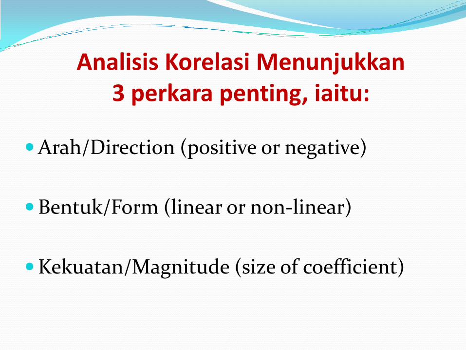
L1. Nyatakan hipotesis
Hipotesis penyelidikan –
Terdapat hubungan yang signifikan antara tahap kepimpinan pengajaran Pengetua dengan prestasi akademik sekolah di Sabah
Hipotesis nol/sifar –
Tiada terdapat hubungan yang signifikan antara tahap kepimpinan pengajaran Pengetua dengan prestasi akademik sekolah di Sabah

L2. TETAPKAN ARAS ALPHA = 0.01/ 0.05/ 0.10, TABURAN PERSAMPELAN, STATISTIK PENGUJIAN
Nilai alpha ditetapkan oleh penyelidik.
Ia merupakan nilai penetapan bahawa penyelidik akan menerima sebarang ralat semasa membuat keputusan pengujian hipotesis tersebut.
Ralat yang sekecil-kecilnya ialah 0.01 (1%), 0.05 (5%) atau 0.10(10%).
Nilai ini juga dipanggil nilai signifikan, aras signifikan, atau aras alpha.

L2. Taburan Persampelan
Taburan yang bersesuaian dengan analisis yang dijalankan. Ia merupakan model taburan korelasi yang mana nilai korelasi itu bertabur secara normal.
Di kawasan kritikal terletak nilai korelasi yang “luar biasa” -> Ha adalah benar
Dikawasan tak kritikal terletak nilai korelasi yang “biasa” -> Ho adalah benar

L3. Nilai Kritikal Nilai kritikal adalah nilai yang menjadi sempadan
bagi kawasan Ho benar dan Hp benar.
Nilai ini merupakan nilai dimana penyelidik meletakkan penetapan sama ada cukup bukti untuk menolak Ho (maka boleh menerima Hp) ataupun tidak cukup bukti menolak Ho (menerima Ho).
Nilai ini bergantung kepada nilai alpha dan arah pengujian hipotesis yang dilakukan.

L4. Nilai Statistik Pengujian Ini adalah nilai yang dikira dan dijadikan bukti
sama ada hipotesis sifar benar atau salah.
Jika nilai statistik pengujian masuk dalam kawasan kritikal maka Ho adalah salah, ditolak dan Hp diterima
Jika nilai statistik pengujian masuk dalam kawasan tak kritikal maka Ho adalah benar, maka terima Ho.

L4. Nilai Statistik Pengujian
r diuji =
r diuji =
16
12
2
nn
d

L5. Membuat Keputusan, Kesimpulan dantafsiran
Jika nilai statistik pengujian masuk dalam kawasan tak kritikal maka Ho adalah benar, maka terima Ho.

L5. Membuat Keputusan, Kesimpulan danTafsiran
Jika nilai statistik pengujian masuk dalam kawasan kritikal maka Ho adalah tak benar, maka Ho ditolak dan seterusnya, Hp diterima (bermakna ada bukti Hp adalah benar)
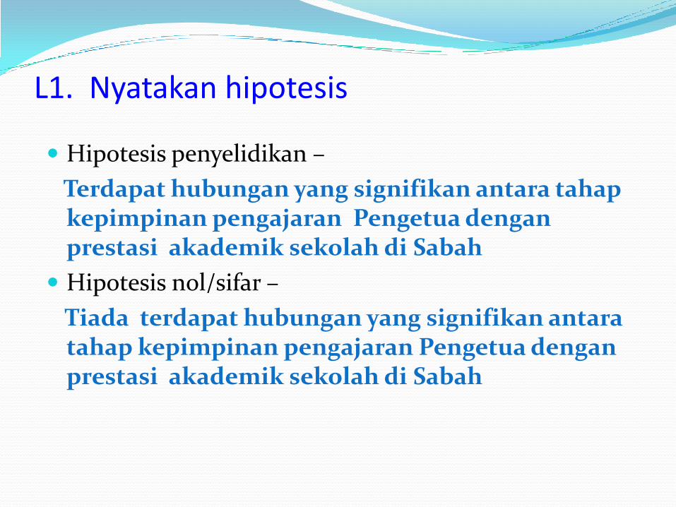
Example of Pearson correlation
Data were collected from a randomly selected sample to
determine relationship between average assignment scores
and test scores in statistics. Distribution for the data is
presented in the table below. Assuming the data are normally
distributed.
1. Calculated an appropriate correlation
coefficient.
2. Describe the nature of relationship
between the two variable.
3. Test the hypothesis on the relationship
at 0.01 level of significance.
Data set:
Assign Test
8.5 88
6 66
9 94
10 98
8 87
7 72
5 45
6 63
7.5 85
5 77

Calculate the test statisticX Y XY X2 Y2
8.5 88 748 72.25 7744
6 66 396 36 4356
9 94 846 81 8836
10 98 980 100 9604
8 87 696 64 7569
7 72 504 49 5184
5 45 225 25 2025
6 63 378 36 3969
7.5 85 637.5 56.25 7225
5 77 385 25 5929

Steps in Hypothesis Testing
3. Determine critical value: df = n – 2, Two-tailed.
r critical= 0.7646
4. Make your decision: r cal > r critical so reject null
hypothesis, accept alternative hypothesis
5. Make conclusion: There is significant relationship
between assignment scores and test scores r (8) =
0.87, p<0.01
1. State the null and alternative hypothesis
HO: ρ p = 0, HA: ρ p ≠ 0
2. Calculate the test statistics: r = .865

Spearman’s rank correlation coefficient
Non parametric method:
Less power but more robust.
Does not assume normal distribution.
The correlation coefficient also varies between -1 and 1

Example of Spearman correlation
Data solicited from a randomly
selected sample of employees
were used to measure
relationship between ratings of
working environment and one’s
work commitment.
1. Calculate and describe the
appropriate correlation coefficient
2. Test the hypothesis on the
relationship at 0.05 level of
significance
ID X Y
1 1 1
2 2 1
3 3 2
4 4 3
5 5 4
6 1 3
7 2 3
8 3 2
9 4 5
10 5 5
11 6 5
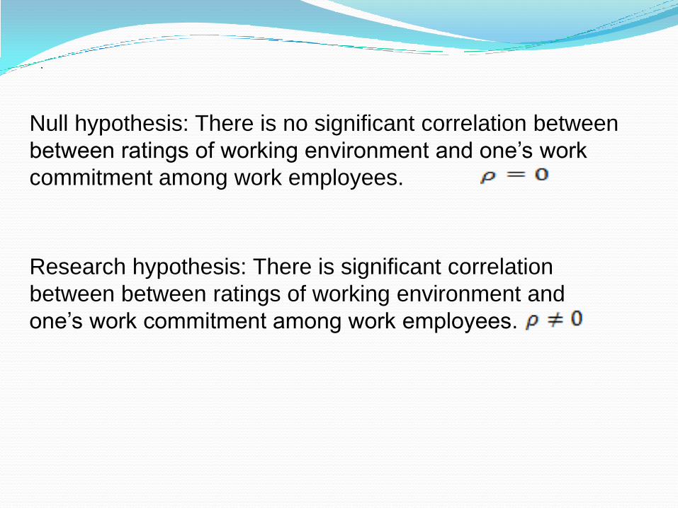
Null hypothesis: There is no significant correlation between
between ratings of working environment and one’s work
commitment among work employees.
Research hypothesis: There is significant correlation
between between ratings of working environment and
one’s work commitment among work employees.
.

Null hypothesis is true
Research hypothesis is true Research hypothesis is true
Determined the critical values in the sampling distribution. Degrees of freedom
From Table r, r = ±.456

Participant Ratings of
work
environment
Ratings of
work
commitment
Rank of
years
Rank
of rating
D D2
1 1 1 1.5 1.5 0 0
2 2 1 3.5 1.5 2 4
3 3 2 5.5 3.5 2 4
4 4 3 7.5 6 1.5 2.25
5 5 4 9.5 8 1.5 2.25
6 1 3 1.5 6 -4.5 20.25
7 2 3 3.5 6 -2.5 6.25
8 3 2 5.5 3.5 2 4
9 4 5 7.5 10 -2.5 6.25
10 5 5 9.5 10 -.5 0.25
11 6 5 11 10 1 1
50.5

Make a decision: Reject the null hypothesishence accept research hypothesis.Conclusion: There was a statistically significantpositive correlation between between ratings ofworking environment and one’s workcommitment among employees (rho = 0.77, p <0.05, N = 11).

r = 1 – 0.229
r = 0.77
There is a positive and strong relationship between ratings
of working environment and one’s work commitment
among employees.
r = 1 - [ 6 D 2 ]
n [ n2 - 1 ]
r = 1 - [ 6(50.5 )]
11 [ 121 - 1 ]
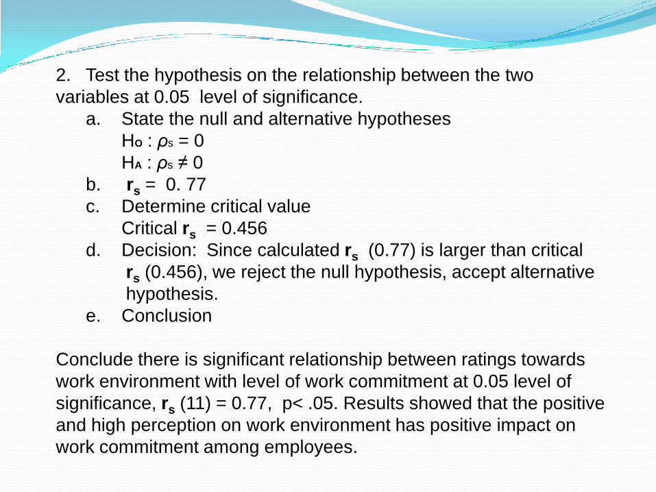
2. Test the hypothesis on the relationship between the two
variables at 0.05 level of significance.
a. State the null and alternative hypotheses
HO : ρs = 0
HA : ρs ≠ 0
b. rs = 0. 77
c. Determine critical value
Critical rs = 0.456
d. Decision: Since calculated rs (0.77) is larger than critical
rs (0.456), we reject the null hypothesis, accept alternative
hypothesis.
e. Conclusion
Conclude there is significant relationship between ratings towards
work environment with level of work commitment at 0.05 level of
significance, rs (11) = 0.77, p< .05. Results showed that the positive
and high perception on work environment has positive impact on
work commitment among employees.

rpb = y1 – y2 [ n1 n2 ]
sy n [ n - 1 ]
Point-biserial Correlation
• Mean of group 1
• Mean of group 2
• Std dev of continuous variable
• No of subjects in group 1
• No of subjects in group 2
• Total no of subjects

Example on Point-biserial
correlation
A psychologist hypothesizes an
association between marital
status (1-single, 2-married) and
need for achievement. A
questionnaire measuring need
for achievement is administered
to married and single people.
1. Calculate the appropriate
correlation coefficient
2. Describe the nature of
relationship between the two
variables.
3. Test the hypothesis on the
relationship at 0.05 level of
significance
Marital status Need for Achievement
2 3
2 7
1 12
1 16
1 24
2 11
1 15
2 10
2 11
1 18
1 22
2 9
1 19
1 17

r = y1 – y2 [ n1 n2 ]
sy n [ n - 1 ]
Point-biserial Correlation
• Mean of married subject = 8.5
• Mean of single subjects = 17.9
• Std dev. of need of achievement scores = 5.89
• No of married subjects = 6 (2)
• No of single subjects = 8 (1)
• Total no of subjects = 14

r = 17.9 – 8.5 [ 8 x 6 ]
5.89 14 [ 14 - 1 ]
Point-biserial Correlation
r pb = 0.82
The mean need for achievement for
single individual is 17.9 and for
married individuals is 8.5. There is a
strong relationship between marital
status and need for achievement.

3. Test the hypothesis on the relationship between the
two variable at 0.05 level of significance.
a. State the null and alternative hypotheses
HO : ρ pb = 0
HA : ρ pb ≠ 0
b. r pb = 0.82
c. Determine critical value: Critical r pb = 0.532
d. Decision: Since calculated r pb (0.82) is greater than
critical value, r pb (0.532), we can reject the null hypothesis
thus accept alternative hypothesis.
e. Conclusion
Therefore there is a significant relationship between
marital status and need for achievement, r pb (12)=.82,
p<0.05. Findings also indicated that single individuals
showed a higher need for achievement compared to
married individuals. Hence marital status has an influence
on one’s need for achievement.

ANALISIS REGRESIAnalisis regresi adalah lanjutan daripada
analisis korelasi dimana sesuatu hubungan telah diperoleh.
Analisis regresi dilaksanakan setelah suatu pola hubungan linear dijangkakan serta suatu pekali ditentukan bagi menunjukkan terdapat hubungan yang linear antara dua pembolehubah.
Selanjutnya bolehlah kita menelah atau meramal sesuatu pembolehubah (p/u criterion) setelah pembolehubah yang kedua (p/u predictive) diketahui.

Prosedurnya ANALISIS REGRESI MUDAH terdiri daripada:
Melakarkan gambarajah sebaran bagi taburan pasangan skor tersebut
Menentukan persamaan bagi garis regresi tersebut
Persamaan ini juga dipanggil model regresi
Persamaan/model bagi garis ini ialah
Y’ = a + bx Dan selanjutnya dengan mengguna
persamaan tersebut, nilai y boleh ditentukan bagi sesuatu nilai x yang telah ditentukan dan juga disebaliknya.
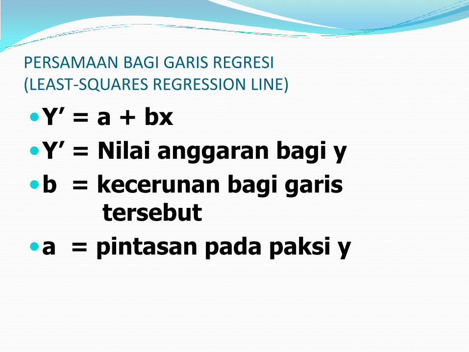
PERSAMAAN BAGI GARIS REGRESI(LEAST-SQUARES REGRESSION LINE)
Y’ = a + bx
Y’ = Nilai anggaran bagi y
b = kecerunan bagi garis tersebut
a = pintasan pada paksi y

b = n [ x y ] - [ x y ]
[ n x2 - ( x)2 ]
KECERUNAN GARIS REGRESI
n = bilangan pasangan skor
x y = jumlah skor x didarab dengan skor y
X = jumlah skor x
y = jumlah skor y
a = PINTASAN PADA PAKSI Y
a = y – b x

Data: Tahap kepemimpinan pengetua dengan persepsi
guru terhadap tahap kepemimpinan pengetua
X Y
12 8
2 3
1 4
6 6
5 9
8 6
4 6
15 22
11 14
13 6
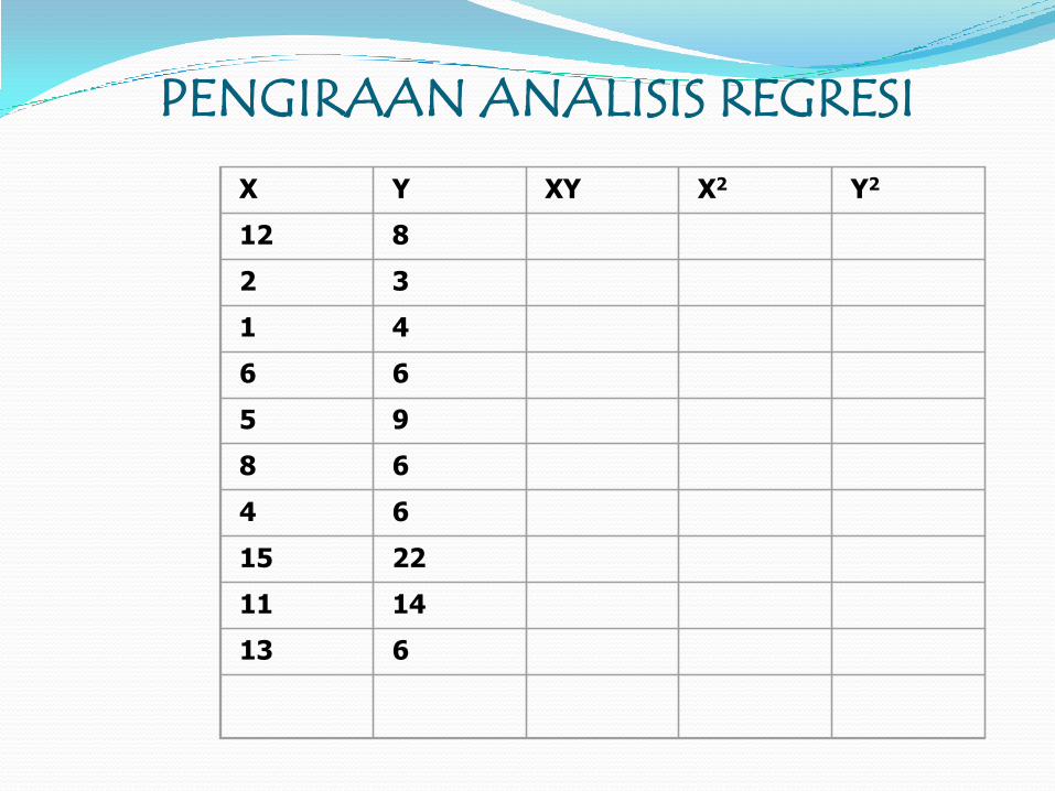
PENGIRAAN ANALISIS REGRESI
X Y XY X2 Y2
12 8
2 3
1 4
6 6
5 9
8 6
4 6
15 22
11 14
13 6

PENGIRAAN ANALISIS REGRESI
X Y XY X2 Y2
12 8 96 144 64
2 3 6 4 9
1 4 4 1 16
6 6 36 36 36
5 9 45 25 81
8 6 48 64 36
4 6 24 16 36
15 22 330 225 484
11 14 154 121 196
13 6 78 169 36
77 84 821 805 994

PERSAMAAN BAGI GARIS REGRESI(LEAST-SQUARES REGRESSION LINE)
Y’ = bx + a
Y’ = Nilai anggran bagi y
b = kecerunan bagi garis tersebut
a= pintasan pada paksi y


r= 0.70. Ini menunjukkan bahawa 49% variasi dalam y
adalah sumbangan daripada X Kecerunannya ialah 0.82Min bagi x ialah 7.7Min bagi y ialah 8.4 a = 2.1 (pintasan di paksi y)Model regresi ialah Y’ = .82x + 2.1 Jika x=7, maka Y’= 7.84 Jika x=10, maka Y’= 10.3 Jika x=14, maka Y’=13.58
54
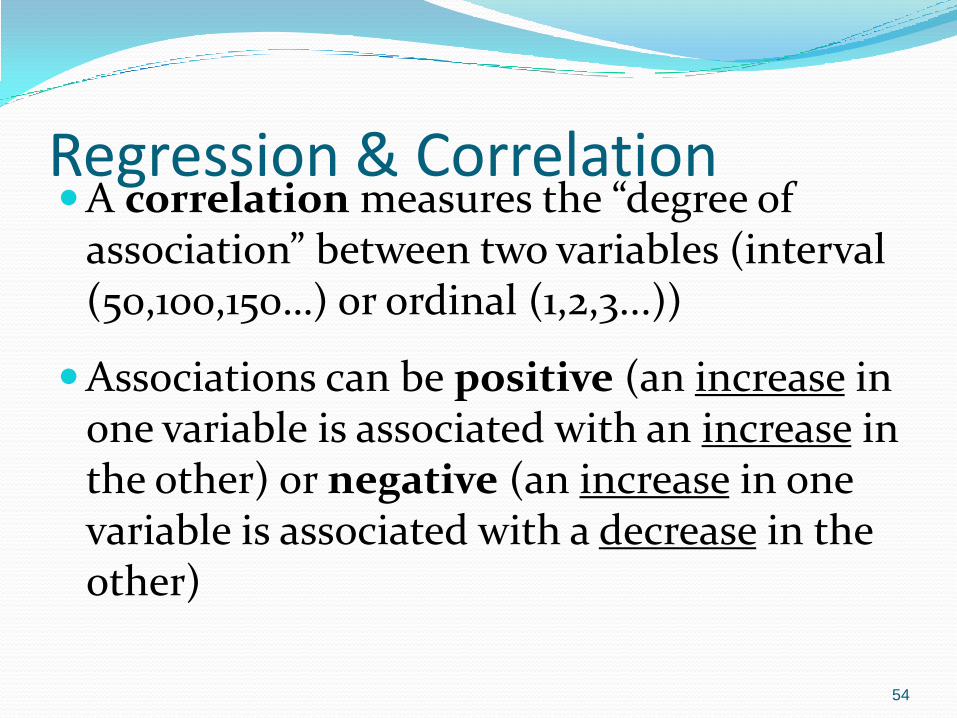
Regression & CorrelationA correlation measures the “degree of
association” between two variables (interval (50,100,150…) or ordinal (1,2,3...))
Associations can be positive (an increase in one variable is associated with an increase in the other) or negative (an increase in one variable is associated with a decrease in the other)

55
Example: Height vs. WeightGraph One: Relationship between Height
and Weight
0
20
40
60
80
100
120
140
160
180
0 50 100 150 200
Height (cms)
Wei
gh
t (k
gs)
Strong positive correlation
between height and weight
Can see how the
relationship works, but
cannot predict one from the
other
If 120cm tall, then how
heavy?

Example: Symptom Index vs Drug A
Strong negative correlation
Can see how relationship works, but cannot make predictions
What Symptom Index might we predict for a standard dose of 150mg?
Graph Two: Relationship between Symptom
Index and Drug A
0
20
40
60
80
100
120
140
160
0 50 100 150 200 250
Drug A (dose in mg)
Sy
mp
tom
In
dex

57
Correlation examples

Regression analysis procedures have as their primary purpose the development of an equation that can be used for predicting values on some DV for all members of a population.
A secondary purpose is to use regression analysis as a means of explaining causal relationships among variables.
Regression

The most basic application of regression analysis is the bivariate situation, to which is referred as simple linear regression, or just simple regression.
Simple regression involves a single IV and a single DV.
Goal: to obtain a linear equation so that we can predict the value of the DV if we have the value of the IV.
Simple regression capitalizes on the correlation between the DV and IV in order to make specific predictions about the DV.

The correlation tells us how much information about the DV is contained in the IV.
If the correlation is perfect (i.e r = ±1.00), the IV contains everything we need to know about the DV, and we will be able to perfectly predict one from the other.
Regression analysis is the means by which we determine the best-fitting line, called the regression line.
Regression line is the straight line that lies closest to all points in a given scatterplot
This line sometimes pass through the centroid of the scatterplot.

“Best fit line”
Allows us to describe relationship between variables more accurately.
We can now predict specific values of one variable from knowledge of the other
All points are close to the line
Graph Three: Relationship between
Symptom Index and Drug A
(with best-fit line)
0
20
40
60
80
100
120
140
160
180
0 50 100 150 200 250
Drug A (dose in mg)
Sy
mp
tom
In
dex
Example: Symptom Index vs Drug A

Graph Four: Relationship between Symptom
Index and Drug B
(with best-fit line)
0
20
40
60
80
100
120
140
160
0 50 100 150 200 250
Drug B (dose in mg)
Sym
pto
m I
nd
ex
We can still predict specific values of one variable from knowledge of the other
Will predictions be as accurate?
Why not?
“Residuals”
Example: Symptom Index vs Drug B

3 important facts about the regression line must be known:The extent to which points are scattered around the line
The slope of the regression line
The point at which the line crosses the Y-axis
The extent to which the points are scattered around the line is typically indicated by the degree of relationship between the IV (X) and DV (Y).
This relationship is measured by a correlation coefficient – the stronger the relationship, the higher the degree of predictability between X and Y.

The degree of slope is determined by the amount of change in Y that accompanies a unit change in X.
It is the slope that largely determines the predicted values of Y from known values for X.
It is important to determine exactly where the regression line crosses the Y-axis (this value is known as the Y-intercept).

The regression line is essentially an equation that express Y as a function of X.
The basic equation for simple regression is:
Y = a + bX
where Y is the predicted value for the DV,
X is the known raw score value on the IV,
b is the slope of the regression line
a is the Y-intercept

Simple Linear Regression
♠ Purpose
To determine relationship between two metric variables
To predict value of the dependent variable (Y) based on
value of independent variable (X)
♠ Requirement :
DV Interval / Ratio
IV Internal / Ratio
♠ Requirement :
The independent and dependent variables are normally
distributed in the population
The cases represents a random sample from the population

Simple RegressionHow best to summarise the data?
0
20
40
60
80
100
120
140
160
180
0 50 100 150 200 250
Drug A (dose in mg)S
ymp
tom
In
dex
0
20
40
60
80
100
120
140
160
0 50 100 150 200 250
Drug A (dose in mg)
Sym
ptom
In
dex
Adding a best-fit line allows us to describe data
simply

Establish equation for the best-fit line:
Y = a + bX
General Linear Model (GLM)How best to summarise the data?
0
20
40
60
80
100
120
140
160
180
200
0 50 100 150 200 250
Where: a = y intercept
(constant)
b = slope of best-fit line
Y = dependent variable
X = independent variable

For simple regression, R2 is the square of the correlation coefficient
Reflects variance accounted for in data by the best-fit line
Takes values between 0 (0%) and 1 (100%)
Frequently expressed as percentage, rather than decimal
High values show good fit, low values show poor fit
Simple RegressionR2 - “Goodness of fit”

R2 = 0
(0% - randomly scattered points, no apparent relationship between X and Y)
Implies that a best-fit line will be a very poor description of data0
50
100
150
200
250
300
0 100 200 300
IV (regressor, predictor)
DV
Simple RegressionLow values of R2

R2 = 1
(100% - points lie directly on the line - perfect relationship between X and Y)
Implies that a best-fit line will be a very good description of data
0
50
100
150
200
250
300
0 100 200 300
IV
DV
0
50
100
150
200
250
0 50 100 150 200 250
IV
DV
Simple RegressionHigh values of R2

0
20
40
60
80
100
120
140
160
180
0 50 100 150 200 250
Drug A (dose in mg)
Sym
pto
m I
nd
ex
0
20
40
60
80
100
120
140
160
0 50 100 150 200 250
Drug B (dose in mg)
Sym
pto
m I
nd
ex
Good fit R2 high
High variance explained
Moderate fit R2
lower
Less variance explained
Simple RegressionR2 - “Goodness of fit”
73
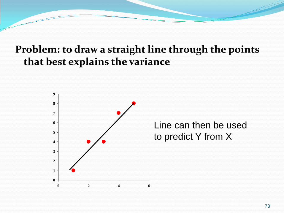
Problem: to draw a straight line through the points that best explains the variance
0
1
2
3
4
5
6
7
8
9
0 2 4 6
Line can then be used
to predict Y from X

74
“Best fit line”
allows us to describe relationship between variables more accurately.
We can now predict specific values of one variable from knowledge of the other
All points are close to the line
Graph Three: Relationship between
Symptom Index and Drug A
(with best-fit line)
0
20
40
60
80
100
120
140
160
180
0 50 100 150 200 250
Drug A (dose in mg)
Sy
mp
tom
In
dex
Example: Symptom Index vs Drug A

75
Establish equation for the best-fit line:
Y = a + bX
Best-fit line same as regression line
b is the regression coefficient for x
x is the predictor or regressor variable for y
Regression

Regression - Types

Step –Descriptive Analysis
Derive Regression / Prediction equation
● Calculate a and b
a = y – b X
Ŷ = a + bX

Example on regression analysis
Data were collected from a randomly
selected sample to determine
relationship between average
assignment scores and test scores in
statistics. Distribution for
the data is presented in the table
below.
1. Calculate coefficient of determination
and the correlation coefficient
2. Determine the prediction equation.
3. Test hypothesis for the slope at 0.05
level of significance
Data set:
Scores
ID Assign Test
1 8.5 88
2 6 66
3 9 94
4 10 98
5 8 87
6 7 72
7 5 45
8 6 63
9 7.5 85
10 5 77
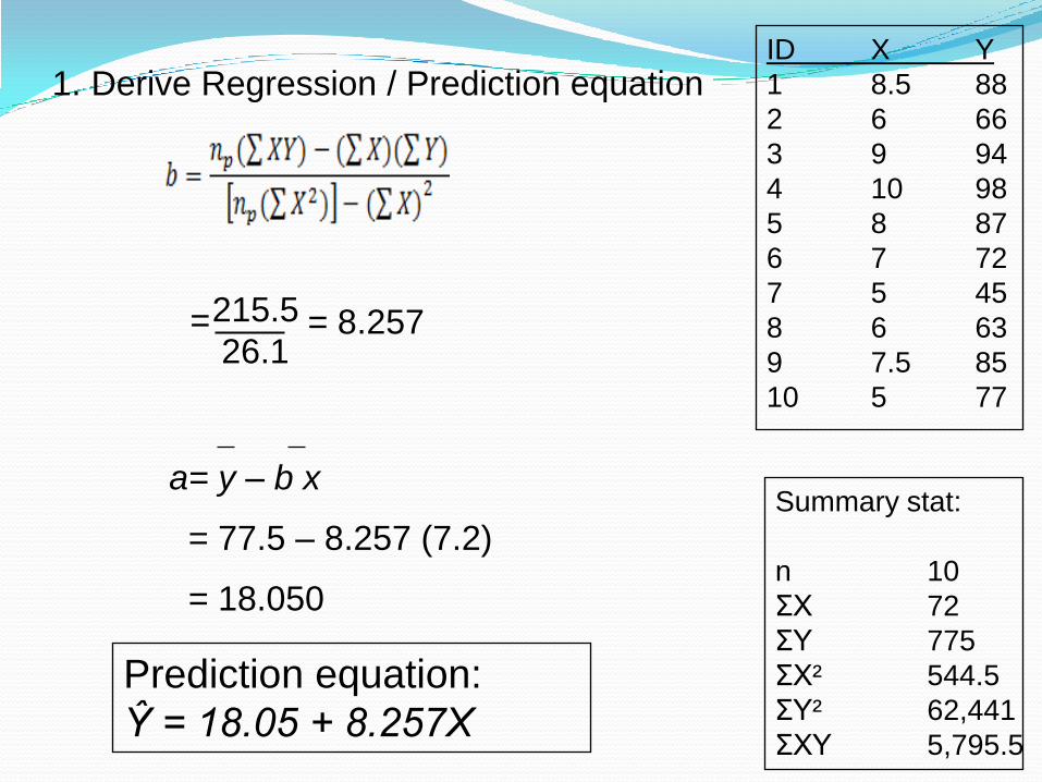
1. Derive Regression / Prediction equation
215.5
26.1= 8.257=
a= y – b x
= 77.5 – 8.257 (7.2)
= 18.050
ID X Y
1 8.5 88
2 6 66
3 9 94
4 10 98
5 8 87
6 7 72
7 5 45
8 6 63
9 7.5 85
10 5 77
Summary stat:
n 10
ΣΧ 72
ΣΥ 775
ΣΧ² 544.5
ΣΥ² 62,441
ΣΧΥ 5,795.5
Prediction equation:
Ŷ = 18.05 + 8.257X

Interpretation of regression equation
Ŷ = 18.05 + 8.257x
For every 1 unit change in X,
Y will change by 8.257 units
ΔX
ΔY18.05

MARITAL SATISFACTION
Parents : X Children : Y
1 3
3 2
7 6
9 7
8 8
4 6
5 3
Mean of X Mean of Y
No of pairs
X Y
X squared X squared
Standard deviation Standard deviation
XY
Example on regression analysis:

1. Derive Regression / Prediction equation
a= y – b x
= 5.00 +.65 (5.29)
= 8.438
Prediction equation:
Ŷ = 8.44 + 65x

Interpretation of regression equation
Ŷ = 8.43 + .65x
For every 1 unit change in X,
Y will change by .65 units
ΔX
ΔY8.43

ANALISIS “CHI-SQUARE”(KUASA-DUA KHI)
Ini juga merupakan analisis hubungan tetapi lebih dikenali sebagai analisis perkaitan (association)
Analisis ini digunakan pakai bagi menentukan perkaitan antara pasangan pembolehubah yang diukur pada skala nominal atau ordinal ataupun jika salah satunya dipadankan dengan data sela dan nisbah.
Dengan itu pembolehubah seperti Bangsa, Jantina, Suka/tidak suka makanan, Tinggi pencapaian/rendah pencapaian, Kebimbangan tinggi/ kebimbangan sederhana/
kebimbangan rendah
Data frekuensi dicerap dengan membilang kejadian (occurance setiap perkara). Sesuai untuk kajian tinjauan
Daripada frekuensi yang dicerap (observed frequency) analisis “chi-square” memberi kita makluman bahawa ada/tiada perkaitan antara kedua-dua pemboleh ubah.

ANALISIS “CHI-SQUARE” (KUASA-DUA KHI)
KATAKANLAH, penyelidik mengumpul maklumat tentang bangsa bagi responden dan juga kategori amalan pemakanan setiap responden,
ATAU penyelidik tinjau pelajar dibeberapa buah sekolah dari segi jantina dan minta/tidak minat kepada aliran sains
ATAU penyelidik tinjau bapa-bapa dan mengumpul maklumat tahap pendidikan (tinggi/ sederhana/ rendah) dan dikaitkan dengan kategori gaji
Bagi ketiga-tiga contoh tersebut analisis yang sesuai dijalankan adalah analisis tak parametrik (analisis kuasa-dua khi)
dan seterusnya dibina jadual kontingensi atau jadual“crosstabulation”.
Daripada frekuensi yang dicerap (observed frequency) analisis “chi-square” memberi kita makluman bahawa ada/tiada perkaitan antara kedua-dua pemboleh ubah.

ANALISIS “CHI-SQUARE”(KUASA-DUA KHI) Terdapat dua cara/kategori – CHI-SQUARE
TEST OF GOODNESS OF FIT dan TEST OF INDEPENDENCE/DEPENDENCE
TEST GOODNESS OF FIT – menjawab persoalan “adakah terdapat perbezaan kadar bagi sesuatu perkara/kejadian/persetujuan”
TEST OF INDEPENDENCE/ DEPENDENCE –menjawab persoalan “adakah terdapat perkaitan/kebersandaran/ hubungan antara dua perkara

ANALISIS “CHI-SQUARE”(KUASA-DUA KHI)
Dapatan bagi analisis ini lazimnya dalam bentuk jadual frekuensi yang dipanggil jadual kontingensi atau jadual “crosstabulation”.
Daripada frekuensi yang dicerap (observed frequency) analisis “chi-square” ini memberi kita makluman bahawa ada/tiada perkaitan yang signifikan antara kedua-dua pembolehubah yang dikaji
Ataupun ada/tiada perbezaan frekuensi yang signifikan antara kategori-kategori yang dikaji.

•Daripada jadual tersebut kita boleh telitikan atau
kajikan sama ada terdapat hubungan atau perkaitan
antara kedua-dua pemboleh ubah tersebut.
•Selanjutnya analisis pengujian hipotesis perlu
dijalankan ia itu untuk menguji terdapatnya perkaitan
antara kedua-dua pemboleh ubah tersebut dengan
signifikan.
•Pengujian hipotesis ini adalah ujian kuasa dua khi.
•Sekiranya, terdapat perkaitan yang signifikan maka
langkah seterusnya adalah dengan menentukan
darjah atau magnitud hubungan tersebut.

•Bagi analisis ini, data adalah dalam bentuk
kekerapan dan sudah semestinya taburan skor
adalah tidak normal.
•Dengan itu taburan ini dipanggil taburan bebas
(distribution-free).
•Ujian ini juga dipanggil ujian tak parametrik oleh
kerana ia tidak bertabur secara normal.
•Sebagai “rule-of-thumb” penggunaan ujian
parametrik digalakkan oleh kerana oleh kerana
“power” atau kekuatannya, walaubagaimana pun jika
data adalah dalam bentuk nominal serta juga terdapat
taburan data yang tidak normal maka ujian tak
parametrik diterima pakai.
•Ujian-ujian parametrik – sign test, Mann-Whitney U
test, Wilcoxon matched-pairs signed ranks, Kruskal-
Wallis, Chi-square.

Uji diri anda!!!-Apakah pengujian statistik yang diperlukan dan seterusnya jalankan analisis
yang diperlukan

EXAMPLE DATA
Parents Marital
Satisfaction
1
3
7
9
8
4
5
Subject
1
2
3
4
5
6
7
Children Marital
Satisfaction
3
2
6
7
8
6
3
Performance
70
80
40
35
50
40
30
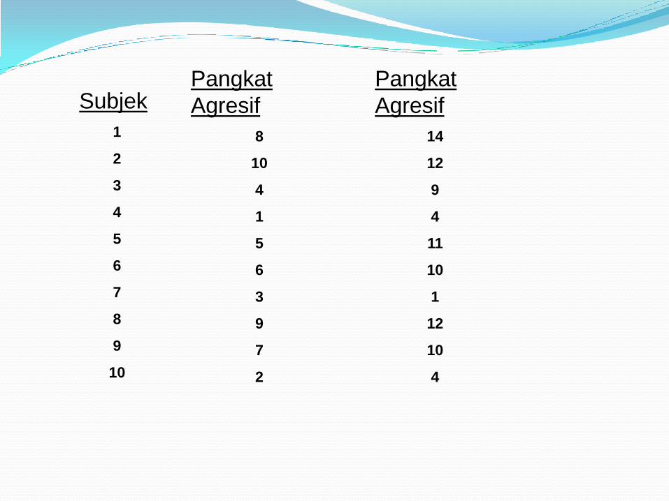
Pangkat
Agresif
8
10
4
1
5
6
3
9
7
2
Subjek
1
2
3
4
5
6
7
8
9
10
Pangkat
Agresif
14
12
9
4
11
10
1
12
10
4

CONTOH DATA 3 Tahap
Kepemimpinan
18
20
24
11
15
16
12
19
17
22
Jantina
1
1
1
1
1
2
2
2
2
2
Stail
Kepimpinan
Autokratik
Autokratik
Autokratik
Demokratik
Demokratik
Demokratik
Demokratik
Autokratik
Demokratik
Autokratik
Persepsi
Prestasi oleh
Guru
20
30
40
85
70
30
80
40
25
75