Statistics of cosmic density profiles from perturbation theory

Statistics of cosmic density profiles from perturbation theory

Francis Bernardeau,1,2 Christophe Pichon,2,3,4 and Sandrine Codis21Institut de Physique Théorique, CEA, IPhT, F-91191 Gif-sur-Yvette,

CNRS, URA 2306, F-91191 Gif-sur-Yvette, France2Institut d’Astrophysique de Paris and UPMC (UMR 7095), 98 bis boulevard Arago, 75014 Paris, France

3Institute of Astronomy, University of Cambridge, Madingley Road,Cambridge CB3 0HA, United Kingdom

4KITP Kohn Hall-4030 University of California, Santa Barbara, California 93106-4030, USA(Received 11 November 2013; published 14 November 2014)

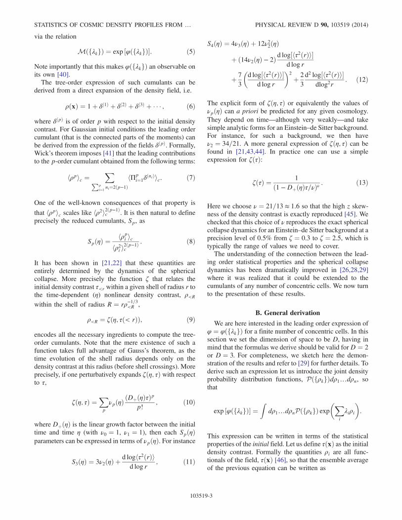
The joint probability distribution function (PDF) of the density within multiple concentric spherical cellsis considered. It is shown how its cumulant generating function can be obtained at tree order in perturbationtheory as the Legendre transform of a function directly built in terms of the initial moments. In the contextof the upcoming generation of large-scale structure surveys, it is conjectured that this result correctlymodels such a function for finite values of the variance. Detailed consequences of this assumption areexplored. In particular the corresponding one-cell density probability distribution at finite variance iscomputed for realistic power spectra, taking into account its scale variation. It is found to be in agreementwith Λ-cold dark matter simulations at the few percent level for a wide range of density values andparameters. Related explicit analytic expansions at the low and high density tails are given. The conditional(at fixed density) and marginal probability of the slope—the density difference between adjacentcells—and its fluctuations is also computed from the two-cell joint PDF; it also compares very well tosimulations. It is emphasized that this could prove useful when studying the statistical properties of voids asit can serve as a statistical indicator to test gravity models and/or probe key cosmological parameters.

DOI: 10.1103/PhysRevD.90.103519 PACS numbers: 98.80.-k, 98.65.-r

I. INTRODUCTION

With new generations of surveys either from ground-based facilities (e.g. BigBOSS, DES, Pan-STARRS, LSST[1]) or space-based observatories (EUCLID [2], SNAP andJDEM [3]), it will be possible to test with unprecedentedaccuracy the details of gravitational instabilities, in par-ticular as it enters the nonlinear regime. These confronta-tions can be used in principle to test the gravity models (seefor instance [4,5]) and/or more generally improve upon ourknowledge of cosmological parameters as detailed in [2].There are only a limited range of quantities that can be

computed from first principles. Next-to-leading-order termsto power spectra and polyspectra have been investigatedextensively over the last few years with the introduction ofnovel methods. Standard perturbation theory calculations, asdescribed in [6], have indeed been extended by the develop-ment of alternative analytical methods that try to improveupon standard calculations. The first significant progress inthis line of calculations in the renormalized perturbationtheory proposition [7] followed by the closure theory [8] andthe time flow equations approach [9]. Latest propositions,namely MPTbreeze [10] and RegPT [11], incorporate2-loop-order calculations and are accompanied by publiclyreleased codes. Recent developments involve the effectivefield theory approaches [12].Alternatively one may look for more global properties of

the fields that capture some aspects of their non-Gaussiannature. A number of tests have been put forward from peak

statistics (see [13]) that set the stage for Gaussian fields,to topological invariants. The latter, introduced for instancein [14] or in [15], aim at producing robust statisticalindicators. This topic was renewed in [16] and [17] withthe introduction of the notion of a skeleton. How suchobservables are affected by weak deviations fromGaussianity was investigated originally in [18] and forinstance more recently in [17,19] with the use of standardtools such as the Edgeworth expansion applied here tomultiple variable distributions. These approaches, althoughpromising, are hampered by the limited range of appli-cability of such expansions and as a consequence have tobe restricted to a limited range of parameters and areusually confined to the nonrare event region.There is however at least one counterexample to that

general statement: the density probability distributionfunctions in concentric cells. As we will show in detailin the following it is possible to get a global picture of whatthe joint density probability distribution function (PDF)should be, including in its rare event tails. The size of thepast surveys prevented an effective use of such statisticaltools. Their current size makes it now possible to try andconfront theoretical calculations with observations.Hence the aim of the paper is to revisit these calculations

and assess their domain of validity with the help ofnumerical simulations.To a large extent, the mathematical foundations of the

calculation of the density probability distribution functions

PHYSICAL REVIEW D 90, 103519 (2014)

1550-7998=2014=90(10)=103519(23) 103519-1 © 2014 American Physical Society

http://dx.doi.org/10.1103/PhysRevD.90.103519




in concentric cells are to be found in early works by Balianand Schaeffer [20], who explored the connection betweencount-in-cell statistics and the properties of the cumulantgenerating functions. In that paper, the shape of the latterwas just assumed without direct connection with thedynamical equations. This connection was established in[21] where it was shown that the leading order generatingfunction of the count-in-cell probability distribution func-tion could be derived from the dynamical equations. Moreprecise calculations were developed in a systematic way in[22] that takes into account filtering effects, as pioneered in[23,24] where the impact of a Gaussian window function ora top-hat window function was taken into account. At thesame time, these predictions were subjected to simulationsand shown to be in excellent agreement with the numericalresults (see for instance [22,25]). We will revisit here thequality of these predictions with the help of more accuratesimulations. In parallel, it was shown that the sameformalism could address more varied situations: large-scalebiasing in [26], projection effects in [27,28]. A compre-hensive presentation of these early works can be foundin [6].Insights into the theoretical foundations of this approach

were presented in [29] that allow to go beyond thediagrammatic approach that was initially employed. Thekey argument is that for densities in concentric cells,the leading contributions in the implementation of thesteepest descent method to the integration over fieldconfigurations should be configurations that are spheri-cally symmetric. One can then take advantage of Gauss’stheorem to map the final field configuration into the initialone with a finite number of initial variables, on a cell-by-cell basis. This is the strategy we adopt below. The purposeof this work is to rederive the fundamental relation that wasobtained by the above mentioned authors, and to revisit thepractical implementation of these calculations alleviatingsome of the shortcuts that were used in the literature.Specifically, the first objective of this paper is to quantity

the sensitivity of the predictions for the one-cell PDF forthe density on the power spectrum shape, its index and thescale dependence of the latter (the so-called runningparameter). The second objective is to show that it ispossible to use the two-cell formalism to derive thestatistical properties of the density slope defined as thedifference of the density in two concentric cells of (possiblyinfinitesimally) close radii and more globally the wholedensity profile. More specifically we show that for suffi-ciently steep power spectra (index less than −1), it ispossible to take the limit of infinitely close top-hat radii anddefine the density slope at a given radius. We can then takeadvantage of this machinery to derive low-order cumulantsof this quantity as well as its complete PDF. Finally thisinvestigation allows us to make a theoretical connectionwith recent efforts (see for instance [30–36]) in exploringthe low density regions and their properties [37] such as the

constrained average slope and its fluctuations given the(possibly low) value of the local density. This opens theway to exploit the properties of low density regions: wewill suggest that the expected profile of low density regionsis in fact a robust tool to use when matching theoreticalpredictions to catalogs.The outline of the paper is the following. In Sec. II we

present the general formalism of how the cumulant gen-erating functions are related to the spherical collapsedynamics. In Sec. III, this relationship is applied to derivethe one-point-density PDF; the sensitivity of the predictionswith scale and with the power spectrum shape is alsoreviewed there. In Sec. IV, we define the density profile andthe slope, and derive its statistical properties. A summaryand discussion on the scope of these results is given in thelast section.

II. THE CUMULANT GENERATINGFUNCTION AT TREE ORDER

Let us first revisit the derivation of the tree-ordercumulant generating functions for densities computed inconcentric cells.

A. Definitions and connections to spherical collapse

We consider a cosmological density field, ρðxÞ, which isstatically isotropic and homogeneous. The average value ofρðxÞ is set to unity. We then consider a random position x0

and n concentric cells of radius Ri centered on x0. Thedensities, ρi, obtained as the density within the radius Ri,

ρi ¼1

4πR3i =3

Zjx−x0j<Ri

d3x ρðxÞ; ð1Þ

form a set of correlated random variables. For a nonlinearlyevolved cosmic density field, they display non-Gaussianstatistical properties. It is therefore natural to define thegenerating function of their joint moments as

MðfλkgÞ ¼X∞pi¼0

hΠiρpii i

Πiλpii

Πipi!; ð2Þ

which can be simply expressed as

MðfλkgÞ ¼�exp

�Xi

λiρi

��: ð3Þ

The generating function, MðfλkgÞ, is a function of then variables λk. A very general theorem (see for instance[38,39]) states that this generating function is closelyrelated to the joint cumulant generating function,

φðfλkgÞ ¼X∞pi¼0

hΠiρpii ic

Πiλpii

Πipi!; ð4Þ

BERNARDEAU, PICHON, AND CODIS PHYSICAL REVIEW D 90, 103519 (2014)

103519-2

via the relation

MðfλkgÞ ¼ exp ½φðfλkgÞ�: ð5Þ

Note importantly that this makes φðfλkgÞ an observable onits own [40].The tree-order expression of such cumulants can be

derived from a direct expansion of the density field, i.e.

ρðxÞ ¼ 1þ δð1Þ þ δð2Þ þ δð3Þ þ � � � ; ð6Þ

where δðpÞ is of order p with respect to the initial densitycontrast. For Gaussian initial conditions the leading ordercumulant (that is the connected parts of the moments) canbe derived from the expression of the fields δðpÞ. Formally,Wick’s theorem imposes [41] that the leading contributionsto the p-order cumulant obtained from the following terms:

hρpic ¼XP

pi¼1

ni¼2ðp−1ÞhΠp

i¼1δðniÞic: ð7Þ

One of the well-known consequences of that property is

that hρpic scales like hρ2i2ðp−1Þc . It is then natural to defineprecisely the reduced cumulants, Sp, as

SpðηÞ ¼hρpi ic

hρ2i i2ðp−1Þc

: ð8Þ

It has been shown in [21,22] that these quantities areentirely determined by the dynamics of the sphericalcollapse. More precisely the function ζ that relates theinitial density contrast τ<r within a given shell of radius r tothe time-dependent (η) nonlinear density contrast, ρ<R

within the shell of radius R ¼ rρ−1=3<R ,

ρ<R ¼ ζðη; τð< rÞÞ; ð9Þ

encodes all the necessary ingredients to compute the tree-order cumulants. Note that the mere existence of such afunction takes full advantage of Gauss’s theorem, as thetime evolution of the shell radius depends only on thedensity contrast at this radius (before shell crossings). Moreprecisely, if one perturbatively expands ζðη; τÞ with respectto τ,

ζðη; τÞ ¼Xp

νpðηÞðDþðηÞτÞp

p!; ð10Þ

where DþðηÞ is the linear growth factor between the initialtime and time η (with ν0 ¼ 1, ν1 ¼ 1), then each SpðηÞparameters can be expressed in terms of νpðηÞ. For instance

S3ðηÞ ¼ 3ν2ðηÞ þd loghτ2ðrÞi

d log r; ð11Þ

S4ðηÞ ¼ 4ν3ðηÞ þ 12ν22ðηÞ

þ ð14ν2ðηÞ − 2Þ d log½hτ2ðrÞi�

d log r

þ 7

3

�d log½hτ2ðrÞi�

d log r

�2

þ 2

3

d2 log½hτ2ðrÞi�dlog2r

: ð12Þ

The explicit form of ζðη; τÞ or equivalently the values ofνpðηÞ can a priori be predicted for any given cosmology.They depend on time—although very weakly—and takesimple analytic forms for an Einstein–de Sitter background.For instance, for such a background, we then haveν2 ¼ 34=21. A more general expression of ζðη; τÞ can befound in [21,43,44]. In practice one can use a simpleexpression for ζðτÞ:

ζðτÞ ¼ 1

ð1 −DþðηÞτ=νÞν: ð13Þ

Here we choose ν ¼ 21=13 ≈ 1.6 so that the high z skew-ness of the density contrast is exactly reproduced [45]. Wechecked that this choice of ν reproduces the exact sphericalcollapse dynamics for an Einstein–de Sitter background at aprecision level of 0.5% from ζ ¼ 0.3 to ζ ¼ 2.5, which istypically the range of values we need to cover.The understanding of the connection between the lead-

ing order statistical properties and the spherical collapsedynamics has been dramatically improved in [26,28,29]where it was realized that it could be extended to thecumulants of any number of concentric cells. We now turnto the presentation of these results.

B. General derivation

We are here interested in the leading order expression ofφ ¼ φðfλkgÞ for a finite number of concentric cells. In thissection we set the dimension of space to be D, having inmind that the formulas we derive should be valid forD ¼ 2or D ¼ 3. For completeness, we sketch here the demon-stration of the results and refer to [29] for further details. Toderive such an expression let us introduce the joint densityprobability distribution functions, PðfρkgÞdρ1…dρn, sothat

exp ½φðfλkgÞ� ¼Z

dρ1…dρnPðfρkgÞ exp�X

i

λiρi

�:

This expression can be written in terms of the statisticalproperties of the initial field. Let us define τðxÞ as the initialdensity contrast. Formally the quantities ρi are all func-tionals of the field, τðxÞ [46], so that the ensemble averageof the previous equation can be written as

STATISTICS OF COSMIC DENSITY PROFILES FROM … PHYSICAL REVIEW D 90, 103519 (2014)

103519-3

exp½φ� ¼Z

DτðxÞPðfτðxÞgÞ exp�X

i

λiρiðfτðxÞgÞ�;

ð14Þ

where we introduced the field distribution function,PðfτðxÞgÞ, and the corresponding measure DðfτðxÞgÞ.These are assumed to be known a priori. They depend onthe initial conditions and in the following we will assumethe initial field is Gaussian distributed [47].We now turn to the calculation of the generating function

at leading order when the overall variance, σ2, at scale Ri, issmall. The idea is to identify the initial field configurationsthat give the largest contribution to this integral. Forconvenience, let us assume that the field τðxÞ can bedescribed with a discrete number of variables τi. ForGaussian initial conditions, the expression of the jointprobability distribution function of τi reads

PðfτkgÞdτ1…dτp ¼ exp ½−ΨðfτkgÞ�ffiffiffiffiffiffiffiffiffiffiffiffiffiffiffiffiffiffiffiffiffiffiffiffið2πÞp= detΞp dτ1…dτp; ð15Þ

with

ΨðfτkgÞ ¼1

2

Xij

Ξijτiτj; ð16Þ

where Ξij is the inverse of the covariance matrix, Σij,defined as

Σij ¼ hτiτji: ð17Þ

The key idea to transform Eq. (14) using Eq. (15) relies onusing the steepest descent method. Details of the validityregime of this approach and its construction can be foundin [29]. The integral we are interested in is then dominatedby a specific field configuration for which the followingstationary conditions are verified:

Xi

λiδρiðfτkgÞ

δτj¼ δ

δτjΨðfτkgÞ; ð18Þ

for any value of j. Up to this point this is a very generalconstruction. Let us now propose a solution to thesestationary equations that is consistent with the class ofspherically symmetric problems we are interested in. Themain point is the following: the configurations that aresolutions of this equation, that is the values of fτkg, dependspecifically on the choice of the functionals ρiðfτkgÞ. Whenthese functionals correspond to spherically symmetricquantities, the corresponding configurations are also likelyto be spherically symmetric. But then Gauss’s theorem ismaking things extremely simple: before shell crossing,each of the final density ρi can indeed be expressed in termsof a single initial quantity, namely the linear density

contrast of the cell centered on x0 that contained the sameamount of matter in the initial density field. We denote τithe corresponding density contrast, which means that,following definition (9), we have

ρi ¼ ζðη; τiÞ; ð19Þ

and τi is the amplitude of the initial density within a specificradius [49], ri, which obeys ri ¼ Riρ

1=Di thanks to mass

conservation. The specificity of this mapping implies inparticular that

δρiðfτkgÞδτj

¼ δijζ0ðτiÞ; ð20Þ

so that the stationary conditions (18) now read

λjζ0ðτjÞ ¼

δ

δτjΨðfτkgÞ: ð21Þ

Note that the no-shell crossing conditions imply that ifRi < Rj, then ri < rj, which in turn implies that

ρi < ρjðRj=RiÞD: ð22Þ

It follows that the parameter space fρkg is not fullyaccessible. In the specific example we explore in thefollowing, this restriction is not significant, but it couldbe in some other cases.We are now close to the requested expression for

φðfλkgÞ as we have

exp ½φðfλkgÞ� ¼Z

dτ1…dτnPðfτkgÞexp�X

i

λiρiðfτkgÞ�:

To get the leading order expression of this form forφðfλkgÞ, using the steepest descent method, one is simplyrequested to identify the quantities that are exponentiated.As a result we have

φðfλkgÞ ¼Xi

λiρi −ΨðfρkgÞ; ð23Þ

where ρi are determined by the stationary conditions (21).The latter can be written equivalently as

λi ¼∂∂ρi ΨðfρkgÞ; ð24Þ

when all quantities are expressed in terms of ρi.Equation (24) is the general expression that we will exploitin the following. Formally, note that (21)–(23) imply thatφðfλkgÞ is the Legendre transform of Ψ when the latter isseen as a function of ρi, that is


103519-4

ΨðfρkgÞ ¼1

2

Xij

ΞijðfρkgÞτðρiÞτðρjÞ; ð25Þ

where the functional form τðρÞ is obtained from theinversion of (19) at a fixed time, and Ξij is the inversematrix of the cross-correlation of the density in cells ofradius Riρ

1=Di [cf. Eq. (17)]:

Σij ¼Dτ�< Riρ

1=Di

�τ�< Rjρ

1=Dj

�E; ð26ÞX

j

ΣijΞjk ¼ δik: ð27Þ

These coefficients therefore depend on the whole set ofboth radii Ri and densities ρi. From the properties ofLegendre transform, it follows in particular that

ρi ¼∂∂λi φðfλkgÞ: ð28Þ

Although known for more than a decade, Eqs. (23)–(28)and their consequences have not been exploited to their fullpower in the literature. This is partially what we intend todo in this paper and in subsequent ones. For now, in order toget better acquainted with this formalism, let us firstexplore some of its properties.

C. General formalism

The relation Eqs. (23)–(28) have been derived forGaussian initial conditions. This eases the presentationbut it is not a key assumption. For instance in Eq. (15),ΨðfτkgÞ does not need to be quadratic in τk as for Gaussianinitial conditions. If the initial conditions were to be non-Gaussian these features would have to be incorporated inthe expression of ΨðfτkgÞ. It would not however changethe functional relation between φðfλkgÞ and ΨðfτkgÞ,provided ΨðfτkgÞ is properly defined when the varianceis taken in its zero limit.One can then observe that the Legendre transform

between these two functions can be inverted [50].Applying the fundamental relation at precisely the initialtime, in a regime where ρi ≈ 1þDþðηÞτi, will give theexpression of the function ΨðfτkgÞ in terms of the initialcumulant generating function.One can actually pursue this idea more generally. Let

us define the nonlinear spherical transform ζρðη; ρ0; η0Þthat gives the value of the density ρ within a givenradius R at time η knowing the density ρ0 at time η0 withinradius R0 ¼ Rðρ=ρ0Þ1=3. It is obtained after τ has beeneliminated in

ζρðη; ρ0; η0Þ ¼ ζðη; τÞ; ð29Þ

ρ0 ¼ ζðη0; τÞ; ð30Þ

where ζ is defined in Eq. (9). Using the form (13), onegets

ζðη; ρ0; η0Þ−1=ν − 1 ¼ DþðηÞDþðη0Þ

ðρ−1=ν0 − 1Þ: ð31Þ

Incidentally we can note that the inverse function isobtained by changing η into η0.Then the general formulation of our result is that the

Legendre transform of the joint cumulant generatingfunction for a choice of radii Rk and taken at time η,which we denote here as Ψðfðρk; RkÞg; ηÞ, can beexpressed in terms of the same Legendre transform takenat any other time, η0,

Ψðfðρk;RkÞg;ηÞ¼Ψ

�ζρðη0;ρk;ηÞ;Rk

ρ1=3k

ζ1=3ρ ðη0;ρk;ηÞ

;η0

�:

ð32Þ

This is a general formalism that encompasses the resultwe just described [51] but can also be applied for anyinitial conditions or any time as it does refer explicitly tothe initial conditions.In this paper we will however use this construction

for initial Gaussian conditions only with explicit use of theexpressions derived in the previous subsection.

D. Scaling relations

It is interesting to note that the cumulant generatingfunction has a simple dependence on the overall amplitudeof the correlators σ20. Let us denote in this subsectionφσ0ðfλkgÞ the value of the cumulant generating function fora fixed value of σ0. It is then straightforward to expressφσ0ðfλkgÞ in terms of φ1ðfλkgÞ, the expression of thegenerating function when σ0 is set to unity. IndeedΨðfρkgÞis inversely proportional to σ20 for fixed values of ρk. As aresult λk scale like 1=σ20 for fixed values of fρkg. Note thatwe have the following identity:

φσ0ðfλkgÞ ¼1

σ20φ1ðfλk=σ20gÞ; ð33Þ

while the variables ρk are independent of σ0.In the upcoming applications we will make use of this

property as we will keep the overall normalization as a freeparameter—that will eventually be adjusted on numericalresults, but will use the structural form of φ1ðfλkgÞ aspredicted from the general theory. In particular this struc-tural form depends on the specific shape of the powerspectrum through the cross-correlation matrix Σij.


103519-5

E. The one-cell generating function

Turning back to the application of Eqs. (23)–(28), oneobvious simple application corresponds to the one-cellcharacteristic function. In this case

ΨðρÞ≡ 1

2σ2ðRρ1=DÞ τðρÞ2; ð34Þ

where

σ2ðrÞ ¼ hτð< rÞτð< rÞi: ð35Þ

The Legendre transform is then straightforward and φðλÞtakes the form

φðλÞ ¼ λρ −1

2σ2ðRρ1=DÞ τðρÞ2; ð36Þ

with ρ computed implicitly as a function of λ via Eq. (24).One way of rewriting this equation is to define τeff ¼τσðRÞ=σðRρ1=3Þ and the function ζeffðτeffÞ through theimplicit form,

ζeffðτeffÞ ¼ ζðτÞ ¼ ζ

�τeff

σðRζ1=Deff ÞσðRÞ

�: ð37Þ

Then the expression of φðλÞ is given by

φðλÞ ¼ λρ −1

2σ2ðRÞ τ2eff ; ð38Þ

with the stationary condition

τeff ¼ λσ2ζ0effðτÞ: ð39Þ

In [22], the expression of the cumulant generating functionwas presented with this form. This is also the functionalform one gets when one neglects the filtering effects (aswas initially done in [21]) or for the so-called nonlinearhierarchical model used in [52]. Note that it is not possiblehowever to use such a remapping for more than one cell.Note finally that this is a precious formulation for practicalimplementations, as one may rely on fitted forms for ζeff toconstruct the generating function φðλÞ while preserving itsanalytical properties. It is indeed always possible, once onehas been able to numerically compute φðλÞ for specificvalues of λ, to define ζeff by Legendre transform andconstruct a fitted form with low-order polynomials whilethis is not possible for φðλÞ which exhibits nontrivialanalytical properties as we will see later on. This approachwas used in [28]. It is also this procedure we use in Sec. IVfor constructing the profile PDF.

F. Recovering the PDF via inverseLaplace transform

In the following we will exploit the expression for thecumulant generating function to get the one-point and jointdensity PDFs. To avoid confusion with the variables ρi thatappear in the expression of Ψ, we will use the superscriptbto denote measurable densities, the PDF of which we wishto compute.In general, the joint density PDF, P ¼ Pðρ1;…; ρnÞ,

that gives the probability that the densities within a setof n concentric cells of radii R1;…; Rn are ρ1;…; ρn withindρ1…dρn is given by

P ¼Z þi∞

−i∞

dλ12πi

� � � dλn2πi

exp

�−Xi

λiρi þ φðfλkÞg�: ð40Þ

where the integration in λi should be performed in thecomplex plane so as to maximize convergence. This equa-tion defines the inverse Laplace transform of the cumulantgenerating function [53]. In the one-cell case, Eq. (40)simply reads

Pðρ1Þ ¼Z þi∞

−i∞

dλ12πi

expð−λ1ρ1 þ φðλ1ÞÞ; ð41Þ

i.e. the PDF is the inverse Laplace transform of the one-variable moment generating function. This inversion isknown to be tricky, and to our knowledge there are noknown general foolproof methods. One practical difficultyis that it generically relies on the analytic continuation of thepredicted cumulant generating function in the complexplane. It is therefore crucial to have a good knowledge ofthe analytic properties of φðλÞ, which is typically difficultsince φðλÞ is defined itself as the Legendre transform ofΨðρÞ. Only a limited set of ΨðρÞ yield analytical φðλÞ,which in turn can be inverse Laplace transformed.

III. THE ONE-POINT PDF

Up to this point, the whole construction presented inthe previous section would be a mere mathematical trick tocompute explicit cumulants for top-hat window functionssparing the pain of lengthy integrations on wave modes.In this paper, we furthermore aim to use the cumulantgenerating function computed in the uniform limit Σij → 0as an approximate form for the exact generating functionwhen the Σij are finite (but small). Note that this is anontrivial extension for which we have no precise math-ematical justifications. It assumes that the global propertiesof φðfλkgÞ—and in particular its analytical properties(which will be of crucial importance in the following)—should be meaningful for finite values of λk, and not only inthe vicinity of fλk ¼ 0g.


103519-6

We now conjecture without further proof that theycorrectly represent the cumulant generating function forfinite values of the variance.

A. General formulas and asymptotic forms

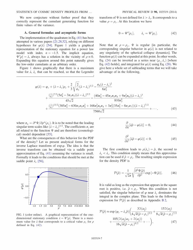
The implementation of the quadrature in Eq. (41) has beenattempted in various papers [21,28,52], relying on differenthypotheses for φðλÞ [54]. Figure 1 yields a graphicalrepresentation of the stationary equation for a power lawmodel with index n ¼ −1.5. The implicit equation,Ψ0½ρ� ¼ λ, always has a solution in the vicinity of ρ ≈ 0.Expanding this equation around this point naturally givesthe low-order cumulants at an arbitrary order.Figure 1 shows graphically that there is a maximum

value for λ, λc that can be reached, so that the Legendre

transform of Ψ is not defined for λ > λc. It corresponds to avalue ρ ¼ ρc. At this location we have

0 ¼ Ψ00½ρc�; λc ¼ Ψ0½ρc�: ð42Þ

Note that at ρ ¼ ρc, Ψ is regular [in particular, thecorresponding singular behavior in φðλÞ is not related toany singularity of the spherical collapse dynamics]. Thefunction φðλÞ can be expanded at this point. In other words,Eq. (24) can be inverted as a series near ðρc; λcÞ [whereEq. (42) holds], and integrated for φðλÞ using Eq. (28). Wegive here a whole set of subleading terms that we will takeadvantage of in the following,

φðλÞ ¼ φc þ ðλ − λcÞρc þ2

3

ffiffiffiffiffi2

π3

sðλ − λcÞ3=2 −

π4ðλ − λcÞ26π23

þð 1π3Þ7=2ð5π24 − 3π3π5Þðλ − λcÞ5=2

45ffiffiffi2

p −ð40π34 − 45π3π5π4 þ 9π23π6Þðλ − λcÞ3

810π53

þð 1π3Þ13=2ð385π44 − 630π3π5π

24 þ 168π23π6π4 þ 3π23ð35π25 − 8π3π7ÞÞðλ − λcÞ7=2

7560ffiffiffi2

p þ � � � ; ð43Þ

where πn ¼ ∂nΨ=∂ρnðρcÞ. It is to be noted that the leadingsingular term scales like ðλ − λcÞ3=2. The coefficients πi areall related to the function Ψ and are therefore (cosmologi-cal) model dependent [55].What are the consequences of this behavior for the PDF

of the density? Let us present analytical forms for theinverse Laplace transform of expφ. The idea is that theinverse transform can be obtained via a saddle pointapproximation of Eq. (41) assuming the variance is small.Formally it leads to the conditions that should be met at thesaddle point λs [56],

∂∂λ ½λρ − φðλÞ� ¼ 0; ð44Þ

∂2

∂λ2 ½λρ − φðλÞ� < 0: ð45Þ

The first condition leads to ρðλsÞ ¼ ρ, the second toλs < λc. This condition simply means that this approxima-tion can be used if ρ < ρc. The resulting simple expressionfor the density PDF is

PðρÞ ¼ 1ffiffiffiffiffiffi2π

pffiffiffiffiffiffiffiffiffiffiffiffiffiffiffi∂2ΨðρÞ∂ρ2

sexp ½−ΨðρÞ�: ð46Þ

It is valid as long as the expression that appears in the squareroot is positive, i.e. ρ < ρc. When this condition is notsatisfied, the singular behavior of φ near λc dominates theintegral in the complex plane. This leads to the followingexpression for PðρÞ as described in Appendix B 2,

PðρÞ ≈ exp ðφc − λcρÞ�

3ℑða32Þ

4ffiffiffiπ

p ðρ − ρcÞ5=2þ

15ℑða52Þ

8ffiffiffiπ

p ðρ − ρcÞ7=2

þ105ðℑða3

2Þa2 þ ℑða7

2ÞÞ

16ffiffiffiπ

p ðρ − ρcÞ9=2þ � � �

�; ð47Þ

1.0 10.05.02.0 20.03.0 30.01.5 15.07.0

0.5

0.0

0.5

'

FIG. 1 (color online). A graphical representation of the one-dimensional stationary condition λ ¼ Ψ0½ρ�. There is a maxi-mum value for λ that corresponds to a critical value ρc for ρdefined in Eq. (42).


103519-7

where aj are the coefficients in front of ðλ − λcÞj in Eq. (43),(e.g. a3=2 ¼ 2=3

ffiffiffiffiffiffiffiffiffiffi2=π3

p) and ℑðÞ is the imaginary part.

Equation (47) has an exponential cutoff at large ρ scaling likeexpðλcρÞ. This property is actually robust and is preservedwhen one performs the inverse Laplace transform for finitevalues of the variance, or even large value of the variance(see [20,57]). It also gives a direct transcription of why φðλÞbecomes singular: for values of λ that are larger than λc, theintegral

RdρPðρÞ expðλρÞ is not converging.

Note that in practice, it is best to rely on an alternativeasymptotic form to Eq. (47) that is better behaved andremains finite for ρ → ρc. It is built in such a way that it hasthe same asymptotic behavior as Eq. (47) at a given order inthe large ρ limit. The following form,

PðρÞ ¼3a3

2exp ðφc − λcρÞ

4ffiffiffiπ

p ðρþ r1 þ r2=ρþ � � �Þ5=2 ; ð48Þ

where the ri parameters are adjusted to fit the results of theprevious expansion, proved very robust. At next-to-leadingorder (NLO) and next-to-next-to-leading order (NNLO) wehave

r1 ¼ −ℑða5

2Þ

ℑða32Þ − ρc; ð49Þ

r2 ¼ −7ð2a2a23

2

þ 2a72a3

2− a25

2

Þ4a23

2

: ð50Þ

However, none of these asymptotic forms are accurate forthe full range of density values; in general one has to relyon numerical integrations in the complex plane which can

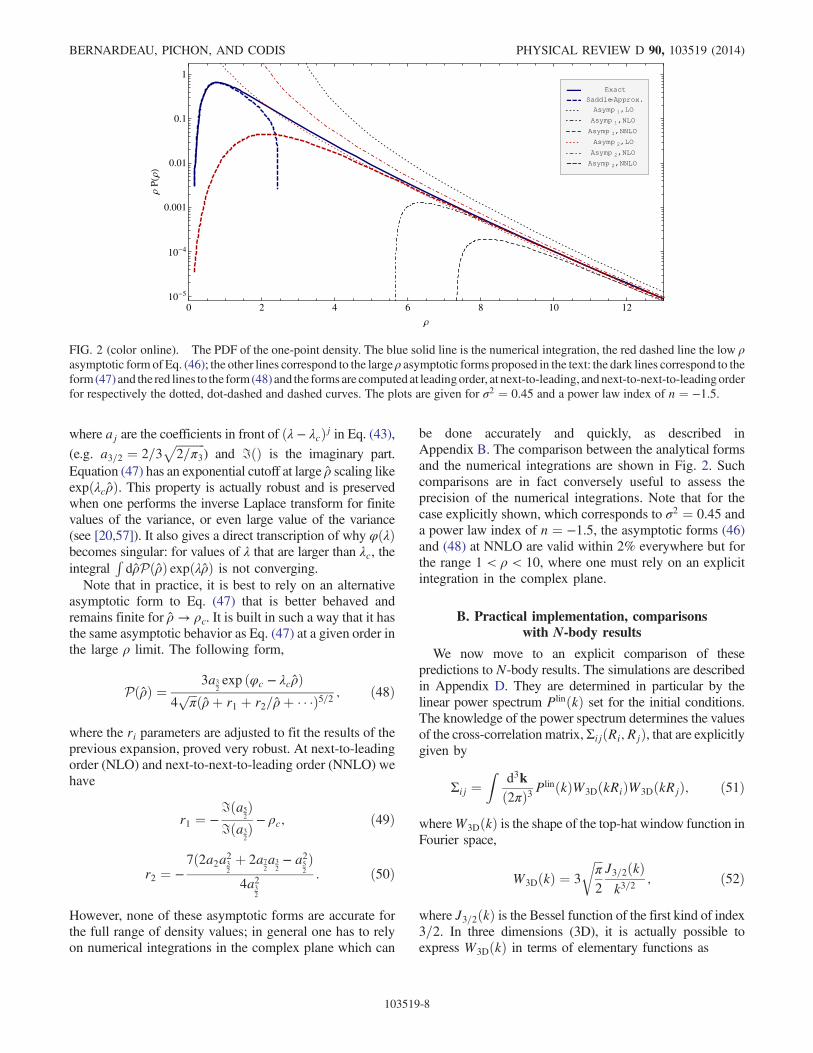
be done accurately and quickly, as described inAppendix B. The comparison between the analytical formsand the numerical integrations are shown in Fig. 2. Suchcomparisons are in fact conversely useful to assess theprecision of the numerical integrations. Note that for thecase explicitly shown, which corresponds to σ2 ¼ 0.45 anda power law index of n ¼ −1.5, the asymptotic forms (46)and (48) at NNLO are valid within 2% everywhere but forthe range 1 < ρ < 10, where one must rely on an explicitintegration in the complex plane.

B. Practical implementation, comparisonswith N-body results

We now move to an explicit comparison of thesepredictions to N-body results. The simulations are describedin Appendix D. They are determined in particular by thelinear power spectrum PlinðkÞ set for the initial conditions.The knowledge of the power spectrum determines the valuesof the cross-correlation matrix,ΣijðRi; RjÞ, that are explicitlygiven by

Σij ¼Z

d3kð2πÞ3 P

linðkÞW3DðkRiÞW3DðkRjÞ; ð51Þ

whereW3DðkÞ is the shape of the top-hat window function inFourier space,

W3DðkÞ ¼ 3

ffiffiffiπ

2

rJ3=2ðkÞk3=2

; ð52Þ

where J3=2ðkÞ is the Bessel function of the first kind of index3=2. In three dimensions (3D), it is actually possible toexpress W3DðkÞ in terms of elementary functions as

0 2 4 6 8 10 1210 5

10 4

0.001

0.01

0.1

1

P

FIG. 2 (color online). The PDF of the one-point density. The blue solid line is the numerical integration, the red dashed line the low ρasymptotic form of Eq. (46); the other lines correspond to the large ρ asymptotic forms proposed in the text: the dark lines correspond to theform(47) and the red lines to the form(48) and the formsare computedat leadingorder, at next-to-leading, andnext-to-next-to-leadingorderfor respectively the dotted, dot-dashed and dashed curves. The plots are given for σ2 ¼ 0.45 and a power law index of n ¼ −1.5.


103519-8

W3DðkÞ ¼3

k2ðsinðkÞ=k − cosðkÞÞ: ð53Þ

For the one-cell case we only need to know the amplitudeand scale dependence of σ2R defined as

σ2ðRÞ ¼Z

d3kð2πÞ3 P

linðkÞW23DðkRÞ: ð54Þ

To a first approximation, σ2ðRÞ can be parametrized witha simple power law σ2ðRÞ ∼ R−ðnsþ3Þ. It is this functionalform which was used in the previous section. The detailedpredictions of the PDF depend however on the precise scaledependence of σ2ðRÞ. Such scale dependence can becomputed numerically from the shape of the powerspectrum but then makes it difficult to derive the functionφðλÞ from the Legendre transform. So in order to retainsimple analytic expressions for the whole cumulant gen-erating function, we adopt a simple prescription for thescale dependence of σ2ðRÞ given by

σ2ðRÞ ¼ 2σ2ðRpÞðR=RpÞn1þ3 þ ðR=RpÞn2þ3

; ð55Þ

where Rp is a pivot scale. Such a parametrization ensuresthat the single-point ΨðρÞ function takes a simple analyticform as it involves the inverse of σ2ðRÞ. Note that ouransatz can be extended to an arbitrary (finite) number ofterms in the denominator.The values of the three parameters, σ2ðRpÞ, n1 and n2 are

then adjusted so that the model reproduces (i) the measuredvariance σ2ðRÞ, (ii) the linear theory index

nðRÞ ¼ −3 −d logðσðRÞÞd logR

; ð56Þ

and (iii) its running parameter

αðRÞ ¼ d logðnðRÞÞd logR

; ð57Þ

at the chosen filtering scale. It is important to point out thatwe do not take the amplitude of σ2ðRÞ as predicted by lineartheory. We consider instead its overall amplitude as a freeparameter and σ2ðRÞ is directly measured from the N-bodyresults. The reason is that using the predicted value ofσ2ðRÞ would simply introduce too large errors and thisdependence can always be scaled out using the relation ofSec. II D [58].In Fig. 3, we explicitly show the comparison between our

predictions following the prescription we just describedto measured PDFs. The predictions show a remarkableagreement with the measured PDF. Recall that only oneparameter, σR, is adjusted to the numerical data. Inparticular the predictions reproduce with an extremely

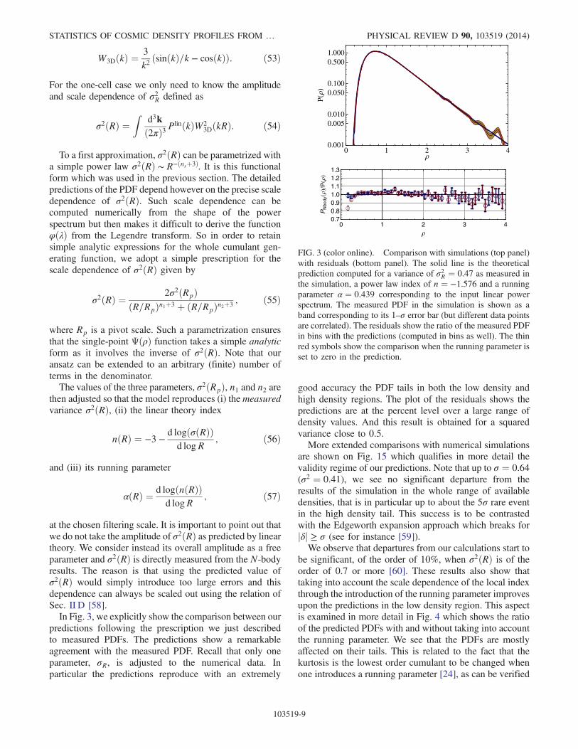
good accuracy the PDF tails in both the low density andhigh density regions. The plot of the residuals shows thepredictions are at the percent level over a large range ofdensity values. And this result is obtained for a squaredvariance close to 0.5.More extended comparisons with numerical simulations

are shown on Fig. 15 which qualifies in more detail thevalidity regime of our predictions. Note that up to σ ¼ 0.64(σ2 ¼ 0.41), we see no significant departure from theresults of the simulation in the whole range of availabledensities, that is in particular up to about the 5σ rare eventin the high density tail. This success is to be contrastedwith the Edgeworth expansion approach which breaks forjδj ≥ σ (see for instance [59]).We observe that departures from our calculations start to

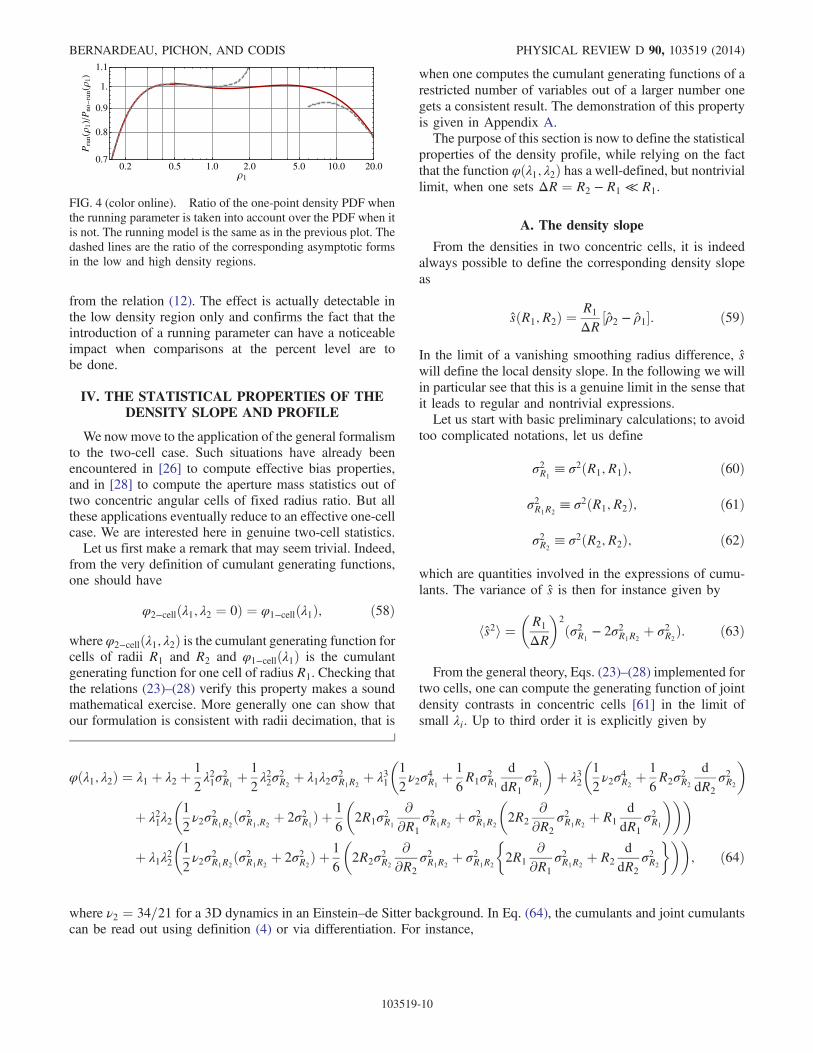
be significant, of the order of 10%, when σ2ðRÞ is of theorder of 0.7 or more [60]. These results also show thattaking into account the scale dependence of the local indexthrough the introduction of the running parameter improvesupon the predictions in the low density region. This aspectis examined in more detail in Fig. 4 which shows the ratioof the predicted PDFs with and without taking into accountthe running parameter. We see that the PDFs are mostlyaffected on their tails. This is related to the fact that thekurtosis is the lowest order cumulant to be changed whenone introduces a running parameter [24], as can be verified

0 1 2 3 40.001

0.0050.010

0.0500.100

0.5001.000

P

0 1 2 3 40.70.80.91.01.11.21.3

PN

body

P

FIG. 3 (color online). Comparison with simulations (top panel)with residuals (bottom panel). The solid line is the theoreticalprediction computed for a variance of σ2R ¼ 0.47 as measured inthe simulation, a power law index of n ¼ −1.576 and a runningparameter α ¼ 0.439 corresponding to the input linear powerspectrum. The measured PDF in the simulation is shown as aband corresponding to its 1–σ error bar (but different data pointsare correlated). The residuals show the ratio of the measured PDFin bins with the predictions (computed in bins as well). The thinred symbols show the comparison when the running parameter isset to zero in the prediction.


103519-9

from the relation (12). The effect is actually detectable inthe low density region only and confirms the fact that theintroduction of a running parameter can have a noticeableimpact when comparisons at the percent level are tobe done.

IV. THE STATISTICAL PROPERTIES OF THEDENSITY SLOPE AND PROFILE

We nowmove to the application of the general formalismto the two-cell case. Such situations have already beenencountered in [26] to compute effective bias properties,and in [28] to compute the aperture mass statistics out oftwo concentric angular cells of fixed radius ratio. But allthese applications eventually reduce to an effective one-cellcase. We are interested here in genuine two-cell statistics.Let us first make a remark that may seem trivial. Indeed,

from the very definition of cumulant generating functions,one should have

φ2−cellðλ1; λ2 ¼ 0Þ ¼ φ1−cellðλ1Þ; ð58Þwhere φ2−cellðλ1; λ2Þ is the cumulant generating function forcells of radii R1 and R2 and φ1−cellðλ1Þ is the cumulantgenerating function for one cell of radius R1. Checking thatthe relations (23)–(28) verify this property makes a soundmathematical exercise. More generally one can show thatour formulation is consistent with radii decimation, that is

when one computes the cumulant generating functions of arestricted number of variables out of a larger number onegets a consistent result. The demonstration of this propertyis given in Appendix A.The purpose of this section is now to define the statistical

properties of the density profile, while relying on the factthat the function φðλ1; λ2Þ has a well-defined, but nontriviallimit, when one sets ΔR ¼ R2 − R1 ≪ R1.

A. The density slope

From the densities in two concentric cells, it is indeedalways possible to define the corresponding density slopeas

sðR1; R2Þ ¼R1

ΔR½ρ2 − ρ1�: ð59Þ

In the limit of a vanishing smoothing radius difference, swill define the local density slope. In the following we willin particular see that this is a genuine limit in the sense thatit leads to regular and nontrivial expressions.Let us start with basic preliminary calculations; to avoid

too complicated notations, let us define

σ2R1≡ σ2ðR1; R1Þ; ð60Þ

σ2R1R2≡ σ2ðR1; R2Þ; ð61Þ

σ2R2≡ σ2ðR2; R2Þ; ð62Þ

which are quantities involved in the expressions of cumu-lants. The variance of s is then for instance given by

hs2i ¼�R1

ΔR

�2

ðσ2R1− 2σ2R1R2

þ σ2R2Þ: ð63Þ

From the general theory, Eqs. (23)–(28) implemented fortwo cells, one can compute the generating function of jointdensity contrasts in concentric cells [61] in the limit ofsmall λi. Up to third order it is explicitly given by

φðλ1; λ2Þ ¼ λ1 þ λ2 þ1

2λ21σ

2R1

þ 1

2λ22σ

2R2

þ λ1λ2σ2R1R2

þ λ31

�1

2ν2σ

4R1

þ 1

6R1σ

2R1

ddR1

σ2R1

�þ λ32

�1

2ν2σ

4R2

þ 1

6R2σ

2R2

ddR2

σ2R2

�þ λ21λ2

�1

2ν2σ

2R1R2

ðσ2R1;R2þ 2σ2R1

Þ þ 1

6

�2R1σ

2R1

∂∂R1

σ2R1R2þ σ2R1R2

�2R2

∂∂R2

σ2R1R2þ R1

ddR1

σ2R1

��þ λ1λ

22

�1

2ν2σ

2R1R2

ðσ2R1R2þ 2σ2R2

Þ þ 1

6

�2R2σ

2R2

∂∂R2

σ2R1R2þ σ2R1R2

2R1

∂∂R1

σ2R1R2þ R2

ddR2

σ2R2

��; ð64Þ

where ν2 ¼ 34=21 for a 3D dynamics in an Einstein–de Sitter background. In Eq. (64), the cumulants and joint cumulantscan be read out using definition (4) or via differentiation. For instance,

0.2 0.5 1.0 2.0 5.0 10.0 20.00.7

0.8

0.9

1.

1.1

1

Pru

n1

Pno

run

1

FIG. 4 (color online). Ratio of the one-point density PDF whenthe running parameter is taken into account over the PDF when itis not. The running model is the same as in the previous plot. Thedashed lines are the ratio of the corresponding asymptotic formsin the low and high density regions.


103519-10

hρ31ic ¼ 3ν2σ4R1

þ σ2R1

R1ddR1

σ2R1; ð65Þ

hρ21ρ2ic ¼ ν2σ2R1R2

ðσ2R1R2þ 2σ2R1

Þ þ 2

3σ2R1

R1∂∂R1

σ2R1R2

þ 1

3σ2R1R2

�2R2∂∂R2

σ2R1R2þ R1ddR1

σ2R1

�; ð66Þ

and the cumulants hρ1ρ22ic and hρ32ic can be obtainedexchanging the role of R1 and R2. It is then also possibleto derive the explicit form for a number of auto- and cross-cumulants between the density ρ≡ ρ1 in the first cell andthe slope s as defined in (59). For instance,

hρ2sic ¼R1

ΔR½hρ21ρ2ic − hρ31ic�; ð67Þ

hρs2ic ¼�R1

ΔR

�2

½hρ1ρ22ic − 2hρ21ρ2ic þ hρ31ic�; ð68Þ

hs3ic ¼�R1

ΔR

�3

½hρ32ic − 3hρ1ρ22ic þ 3hρ21ρ2ic − hρ31ic�:ð69Þ

Following the one-cell case (see for instance [6]) it ispossible to formally define the reduced cross-correlationsthat are independent on the overall amplitude of the powerspectrum. More precisely, the reduced cross-correlationscan be defined as

Sp0 ¼hρpichρ2ip−1c

; ð70Þ

Spq ¼hρpsqic

hρ2ip−1c hρ sichs2iq−1c; ð71Þ

S0q ¼hsqichs2iq−1c

: ð72Þ

From the previous expressions these quantities can becomputed in the limit of an infinitely small variance.

B. Cumulants and slope in the limit ðΔRÞ=R → 0

Let us now consider the statistical properties of s inthe limit ðΔRÞ=R → 0. To start with, let us compute thevariance of the slope s in the limit ΔR=R → 0. Its varianceis formally given by

hs2i ¼ R21∂2

∂R1∂R2

σ2R1R2jR¼R1¼R2

: ð73Þ

This expression can easily be expressed in terms of thepower spectrum,

hs2i ¼Z

d3kð2πÞ3 P

linðkÞ ~W23DðkRÞ; ð74Þ

where ~W3DðkÞ is the logarithmic derivative of W3DðkÞ,

~W3DðkÞ ¼d

d log kW3DðkÞ; ð75Þ

which for the 3D case can be written,

~W3DðkÞ ¼1

k3½ð9k cosðkÞ þ 3ðk2 − 3Þ sinðkÞ�: ð76Þ

Note that for a power law spectrum of index ns this varianceis only defined when ns < −1. For practical application tocosmological models that resemble the concordant model,the effective index ns decreases to −3 at small scales andthe variance of s is always finite. This property howeversuggests that the amplitude of the slope fluctuations couldbe dominated by density fluctuations at scales significantlysmaller than the smoothing radius if the latter is largeenough. This is not expected to be the case however forthe filtering scales we explore in this investigation. Moreprecisely, provided the power spectrum index is in therange ½−3;−1�, the amplitude of the variance of s can beexpressed in terms of the variance of the density as

hs2i ¼ σ2Rnsðns þ 3Þðns þ 5Þ

4ðns þ 1Þ : ð77Þ

Let us now see how the whole statistical properties ofthe variable s can be derived from our formalism. Let usfirst explore the consequence of the change of variable,ðρ1; ρ2Þ → ðρ; sÞ. Instead of describing the joint PDF as afunction of the associated variables λ1 and λ2 we can buildit with the variable associated to ρ and s. Noting thatλ1ρ1 þ λ2ρ2 can be written as

λ1ρ1 þ λ2ρ2 ¼ ðλ1 þ λ2Þρ1 þΔRR1

λ2s; ð78Þ

as a consequence, the joint cumulant generating function ofρ1 and s is given by φðλ1; λ2Þ when written as a function of

λ ¼ λ1 þ λ2; μ ¼ ΔRR1

λ2; ð79Þ

which are the variables associated with the Laplace andinverse Laplace transform of Pðρ1; sÞ. One can also checkthat, following this definition, φðλ; μÞ is the Legendretransform of Ψðρ1; s ¼ ðρ2 − ρ1ÞR1=ΔRÞ.Let us then explore the whole statistical properties of s in

the limit of a vanishing radius difference ðΔRÞ=R → 0.First note that the reduced skewness of s is still finite [62]and has a nontrivial value. It is given by


103519-11

SΔR→003 ¼2þ

∂∂R1

σ2R1R2

R1∂2∂R1∂R2σ2R1R2

R¼R1¼R2

ð6ν2−ð ~nþ3ÞÞ; ð80Þ

where the effective index, ~n, is defined as

1

hs2id

d logRhs2i ¼ −ð ~nþ 3Þ: ð81Þ

We will see in the following that this feature, the fact thatreduced cumulants remain finite, extends to the wholegenerating function.

C. Analytic properties of φðλ;μÞLet us now turn to the full analytical properties of

φðλ; μÞ, for a finite radius difference to start with, and thenin the limit of vanishing radius difference. It is to be notedthat, as for the one-cell case, not all values of λ and μare accessible. This is due to the fact that the ρi –λi

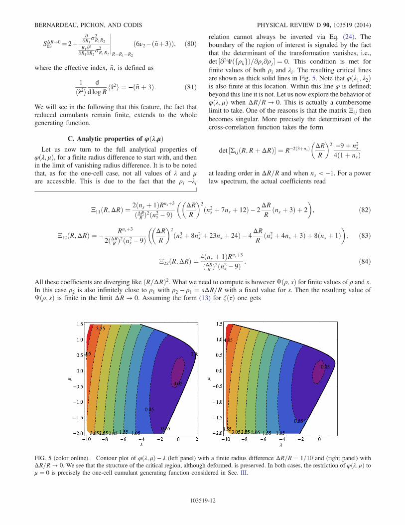
relation cannot always be inverted via Eq. (24). Theboundary of the region of interest is signaled by the factthat the determinant of the transformation vanishes, i.e.,det ½∂2ΨðfρkgÞ=∂ρi∂ρj� ¼ 0. This condition is met forfinite values of both ρi and λi. The resulting critical linesare shown as thick solid lines in Fig. 5. Note that φðλ1; λ2Þis also finite at this location. Within this line φ is defined;beyond this line it is not. Let us now explore the behavior ofφðλ; μÞ when ΔR=R → 0. This is actually a cumbersomelimit to take. One of the reasons is that the matrix Ξij thenbecomes singular. More precisely the determinant of thecross-correlation function takes the form

det ½ΣijðR;Rþ ΔRÞ� ¼ R−2ð3þnsÞ�ΔRR

�2 −9þ n2s4ð1þ nsÞ

at leading order in ΔR=R and when ns < −1. For a powerlaw spectrum, the actual coefficients read

Ξ11ðR;ΔRÞ ¼2ðns þ 1ÞRnsþ3

ðΔRR Þ2ðn2s − 9Þ��

ΔRR

�2

ðn2s þ 7ns þ 12Þ − 2ΔRR

ðns þ 3Þ þ 2

�; ð82Þ

Ξ12ðR;ΔRÞ ¼ −Rnsþ3

2ðΔRR Þ2ðn2s − 9Þ��

ΔRR

�2

ðn3s þ 8n2s þ 23ns þ 24Þ − 4ΔRR

ðn2s þ 4ns þ 3Þ þ 8ðns þ 1Þ�; ð83Þ

Ξ22ðR;ΔRÞ ¼4ðns þ 1ÞRnsþ3

ðΔRR Þ2ðn2s − 9Þ : ð84Þ

All these coefficients are diverging like ðR=ΔRÞ2. What we need to compute is however Ψðρ; sÞ for finite values of ρ and s.In this case ρ2 is also infinitely close to ρ1 with ρ2 − ρ1 ¼ sΔR=R with a fixed value for s. Then the resulting value ofΨðρ; sÞ is finite in the limit ΔR → 0. Assuming the form (13) for ζðτÞ one gets

FIG. 5 (color online). Contour plot of φðλ; μÞ − λ (left panel) with a finite radius difference ΔR=R ¼ 1=10 and (right panel) withΔR=R → 0. We see that the structure of the critical region, although deformed, is preserved. In both cases, the restriction of φðλ; μÞ toμ ¼ 0 is precisely the one-cell cumulant generating function considered in Sec. III.


103519-12

Ψðρ; sÞ ¼ R3þnsρns=3þðν−2Þ=ν

2ðn2s − 9Þðsþ 3ρÞ2 fs2½ν2n3sðρ1

ν − 1Þ2 þ 3nsð5ν2ðρ1ν − 1Þ2 þ 16νðρ1

ν − 1Þ þ 12Þ

þ4νn2sðρ1ν − 1Þð2νðρ1

ν − 1Þ þ 3Þ þ 36ðνðρ1ν − 1Þ þ 1Þ� þ 9ν2ρ2nsðn2s þ 8ns þ 15Þðρ1

ν − 1Þ2

þ 6sνρðns þ 3Þðρ1ν − 1Þðνn2sðρ1

ν − 1Þ þ nsð5νðρ1ν − 1Þ þ 6Þ þ 6Þg: ð85Þ

The function φðλ; μÞ can then be obtained by Legendretransform. Like for the one-cell case, the transformationbecomes critical when the inversion of the stationarycondition is singular. For the new variables, it is alsooccurring when the determinant of the second derivatives ofΨ vanishes,

det

�∂2Ψðρ; sÞ∂ρ∂s

�¼ 0; ð86Þ

which generalizes the condition (42). This conditiondefines the location of the critical line which can thenbe visualized in the λ − μ plane (thick lines in Fig. 5). Notethat the no-shell crossing condition, which in this limitreads s > −3ρ, is located beyond this critical line and istherefore not relevant.In the regular region, the contour lines of φðλ; μÞ are

shown in Fig. 5 for both a finite ratio ΔR=R and when it isinfinitely small. This figure explicitly shows in particularthat the limit ΔR → 0 is nonpathological, in the sense thatthe location of the critical line and the actual value ofthe cumulant generating function converge to well-definedvalues in that limit. The convergence is however not veryrapid and in practice we will use finite differences forcomparisons with simulations.Finally, to conclude this subsection we also compare

these contour plots with those measured in simulations.There, one actually computes the explicit sum

exp½φðλ; μÞ� ¼ 1

Nx

Xx

expðλρx þ μsxÞ; ð87Þ

where ρx and sx are the measured values of ρ and s in a cellcentered on x (in practice on grid points) and Nx is thenumber of points used (see Appendix D for details). Thenφðλ; μÞ is always well defined, irrespective of the values ofλ and μ. To detect the location of a critical line one shouldthen rely on the properties it is associated with. From theanalysis of the one-cell case it appears that for λ > λc, φðλÞis ill defined because

RPðρÞ expðλρÞdρ diverges. More

precisely when λ → λc the value of φðλÞ becomes domi-nated by the rare event tail. It makes such a quantity verysensitive to cosmic variance and in practice the critical lineposition is therefore associated with a diverging cosmicvariance. In the two-cell case, we encounter the sameeffects. To locate we therefore simply cut out part of theðλ − μÞ plane for which the measured variance of φðλ; μÞexceeds a significant fraction of its measured value. We set

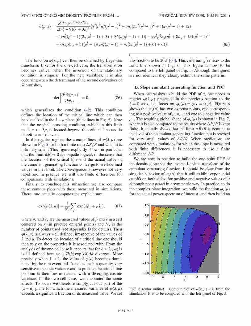
this fraction to be 20% [63]. This criterium give rises to thesolid line shown in Fig. 6. This figure is now to becompared to the left panel of Fig. 5. Although the figuresare not identical they clearly exhibit the same patterns.

D. Slope cumulant generating function and PDF

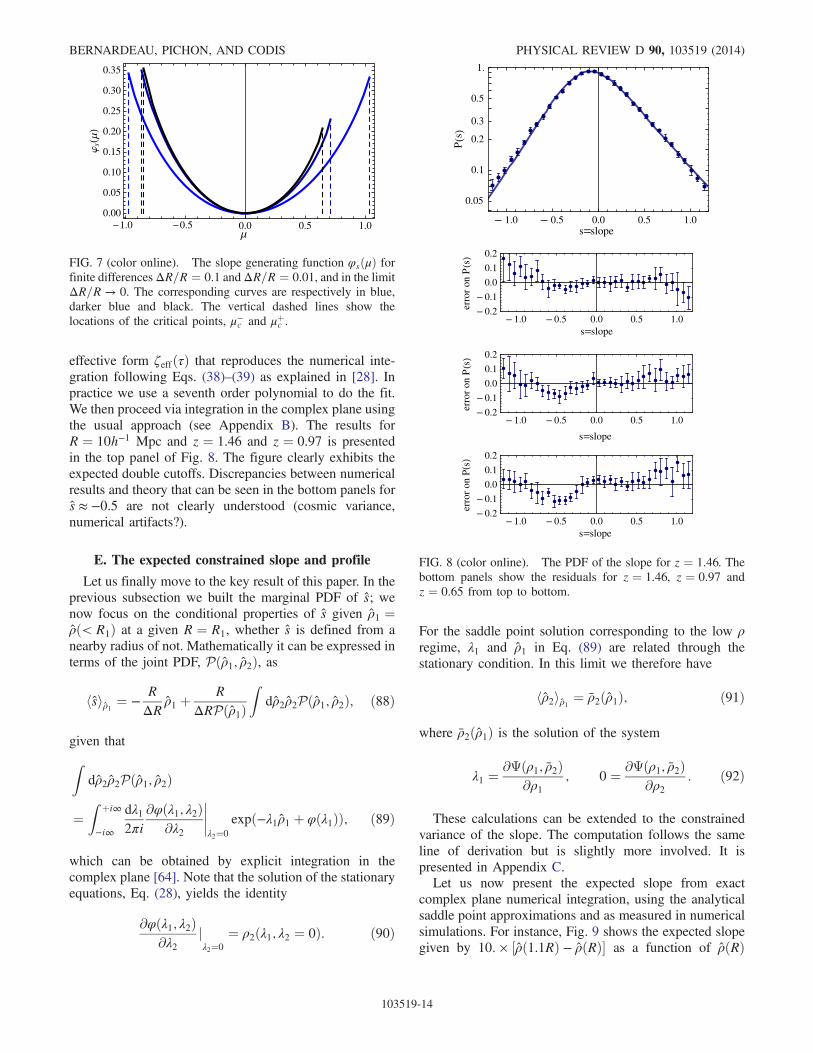
When one wishes to build the PDF of s, one needs torestrict φðλ; μÞ presented in the previous section to theλ ¼ 0 axis, i.e. focus on φsðμÞ≡ φðλ ¼ 0; μÞ. Figure 6shows that φsðμÞ has two extrema points, one correspond-ing to a positive value of μ, μþc , and one to a negative valueμ−c . The resulting global shape of φsðμÞ is shown in Fig. 7,where it is also compared to the results whereΔR=R is keptfinite. It actually shows that the limit ΔR=R is genuine atthe level of the cumulant generating function but is reachedfor very small values of ΔR=R. When predictions arecompared with simulations for which the slope is measuredwith finite differences, it is necessary to use a finitedifference ΔR.We are now in position to build the one-point PDF of

the density slope via the inverse Laplace transform of thecumulant generating function. It should be clear from thesingular behavior of φsðμÞ that it will exhibit exponentialcutoffs on both sides, for positive and negative values of salthough not a priori in a symmetric way. In practice, to dothe complex plane integration, we build the function φsðμÞfor the actual power spectrum of interest, and then build an

FIG. 6 (color online). Contour plot of φðλ; μÞ − λ, from thesimulation. It is to be compared with the left panel of Fig. 5.


103519-13

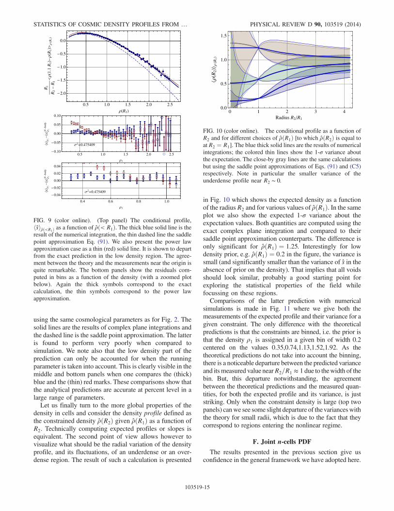
effective form ζeffðτÞ that reproduces the numerical inte-gration following Eqs. (38)–(39) as explained in [28]. Inpractice we use a seventh order polynomial to do the fit.We then proceed via integration in the complex plane usingthe usual approach (see Appendix B). The results forR ¼ 10h−1 Mpc and z ¼ 1.46 and z ¼ 0.97 is presentedin the top panel of Fig. 8. The figure clearly exhibits theexpected double cutoffs. Discrepancies between numericalresults and theory that can be seen in the bottom panels fors ≈ −0.5 are not clearly understood (cosmic variance,numerical artifacts?).

E. The expected constrained slope and profile

Let us finally move to the key result of this paper. In theprevious subsection we built the marginal PDF of s; wenow focus on the conditional properties of s given ρ1 ¼ρð< R1Þ at a given R ¼ R1, whether s is defined from anearby radius of not. Mathematically it can be expressed interms of the joint PDF, Pðρ1; ρ2Þ, as

hsiρ1 ¼ −RΔR

ρ1 þR

ΔRPðρ1ÞZ

dρ2ρ2Pðρ1; ρ2Þ; ð88Þ

given thatZdρ2ρ2Pðρ1; ρ2Þ

¼Z þi∞

−i∞

dλ12πi

∂φðλ1; λ2Þ∂λ2

λ2¼0

expð−λ1ρ1 þ φðλ1ÞÞ; ð89Þ

which can be obtained by explicit integration in thecomplex plane [64]. Note that the solution of the stationaryequations, Eq. (28), yields the identity

∂φðλ1; λ2Þ∂λ2 j

λ2¼0

¼ ρ2ðλ1; λ2 ¼ 0Þ: ð90Þ

For the saddle point solution corresponding to the low ρregime, λ1 and ρ1 in Eq. (89) are related through thestationary condition. In this limit we therefore have

hρ2iρ1 ¼ ρ2ðρ1Þ; ð91Þ

where ρ2ðρ1Þ is the solution of the system

λ1 ¼∂Ψðρ1; ρ2Þ

∂ρ1 ; 0 ¼ ∂Ψðρ1; ρ2Þ∂ρ2 : ð92Þ

These calculations can be extended to the constrainedvariance of the slope. The computation follows the sameline of derivation but is slightly more involved. It ispresented in Appendix C.Let us now present the expected slope from exact

complex plane numerical integration, using the analyticalsaddle point approximations and as measured in numericalsimulations. For instance, Fig. 9 shows the expected slopegiven by 10: × ½ρð1.1RÞ − ρðRÞ� as a function of ρðRÞ

1.0 0.5 0.0 0.5 1.0

0.05

0.1

0.2

0.3

0.5

1.

s slope

Ps

1.0 0.5 0.0 0.5 1.00.2

0.1

0.0

0.1

0.2

s slope

erro

ron

Ps

1.0 0.5 0.0 0.5 1.00.2

0.1

0.0

0.1

0.2

s slope

erro

ron

Ps

1.0 0.5 0.0 0.5 1.00.2

0.1

0.0

0.1

0.2

s slope

erro

ron

Ps

FIG. 8 (color online). The PDF of the slope for z ¼ 1.46. Thebottom panels show the residuals for z ¼ 1.46, z ¼ 0.97 andz ¼ 0.65 from top to bottom.

1.0 0.5 0.0 0.5 1.00.00

0.05

0.10

0.15

0.20

0.25

0.30

0.35

s

FIG. 7 (color online). The slope generating function φsðμÞ forfinite differencesΔR=R ¼ 0.1 andΔR=R ¼ 0.01, and in the limitΔR=R → 0. The corresponding curves are respectively in blue,darker blue and black. The vertical dashed lines show thelocations of the critical points, μ−c and μþc .


103519-14

using the same cosmological parameters as for Fig. 2. Thesolid lines are the results of complex plane integrations andthe dashed line is the saddle point approximation. The latteris found to perform very poorly when compared tosimulation. We note also that the low density part of theprediction can only be accounted for when the runningparameter is taken into account. This is clearly visible in themiddle and bottom panels when one compares the (thick)blue and the (thin) red marks. These comparisons show thatthe analytical predictions are accurate at percent level in alarge range of parameters.Let us finally turn to the more global properties of the

density in cells and consider the density profile defined asthe constrained density ρðR2Þ given ρðR1Þ as a function ofR2. Technically computing expected profiles or slopes isequivalent. The second point of view allows however tovisualize what should be the radial variation of the densityprofile, and its fluctuations, of an underdense or an over-dense region. The result of such a calculation is presented

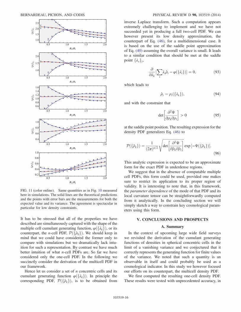
in Fig. 10 which shows the expected density as a functionof the radius R2 and for various values of ρðR1Þ. In the sameplot we also show the expected 1-σ variance about theexpectation values. Both quantities are computed using theexact complex plane integration and compared to theirsaddle point approximation counterparts. The difference isonly significant for ρðR1Þ ¼ 1.25. Interestingly for lowdensity prior, e.g. ρðR1Þ ¼ 0.2 in the figure, the variance issmall (and significantly smaller than the variance of s in theabsence of prior on the density). That implies that all voidsshould look similar, probably a good starting point forexploring the statistical properties of the field whilefocussing on these regions.Comparisons of the latter prediction with numerical

simulations is made in Fig. 11 where we give both themeasurements of the expected profile and their variance for agiven constraint. The only difference with the theoreticalpredictions is that the constraints are binned, i.e. the prior isthat the density ρ1 is assigned in a given bin of width 0.2centered on the values 0.35,0.74,1.13,1.52,1.92. As thetheoretical predictions do not take into account the binning,there is a noticeable departure between the predicted varianceand itsmeasured value nearR2=R1 ≈ 1 due to thewidth of thebin. But, this departure notwithstanding, the agreementbetween the theoretical predictions and the measured quan-tities, for both the expected profile and its variance, is juststriking. Only when the constraint density is large (top twopanels) canwe see some slight departure of thevarianceswiththe theory for small radii, which is due to the fact that theycorrespond to regions entering the nonlinear regime.

F. Joint n-cells PDF

The results presented in the previous section give usconfidence in the general framework we have adopted here.

0 1 2 3 40.0

0.5

1.0

1.5

Radius R2 R1

R2

R1

FIG. 10 (color online). The conditional profile as a function ofR2 and for different choices of ρðR1Þ [to which ρðR2Þ is equal toat R2 ¼ R1]. The blue thick solid lines are the results of numericalintegrations; the colored thin lines show the 1-σ variance aboutthe expectation. The close-by gray lines are the same calculationsbut using the saddle point approximations of Eqs. (91) and (C5)respectively. Note in particular the smaller variance of theunderdense profile near R2 ∼ 0.

0.5 1.0 1.5 2.0 2.5

2.0

1.5

1.0

0.5

0.0

R1

R1

R2

R1

1.1

R1

R1

R1

0.5 1.0 1.5 2.0 2.50.10

0.05

0.00

0.05

0.10

1

s1

s1

Nbo

dy

2 0.475409

0.4 0.6 0.8 1.0

0.04

0.02

0.00

0.02

0.04

1

s1

s1

Nbo

dy

2 0.475409

FIG. 9 (color online). (Top panel) The conditional profile,hsiρð<R1Þ as a function of ρð< R1Þ. The thick blue solid line is theresult of the numerical integration, the thin dashed line the saddlepoint approximation Eq. (91). We also present the power lawapproximation case as a thin (red) solid line. It is shown to departfrom the exact prediction in the low density region. The agree-ment between the theory and the measurements near the origin isquite remarkable. The bottom panels show the residuals com-puted in bins as a function of the density (with a zoomed plotbelow). Again the thick symbols correspond to the exactcalculation, the thin symbols correspond to the power lawapproximation.


103519-15

It has to be stressed that all of the properties we havedescribed are simultaneously captured with the shape of themultiple cell cumulant generating function, φðfλkgÞ, or itscounterpart, the n-cell PDF, PðfρkgÞ. We should keep inmind that we could have considered the former only tocompare with simulations but we dramatically lack intu-ition for such a representation. By contrast we have muchbetter intuition of what n-cell PDFs are. So far we haveconsidered only the one-cell PDF. In the following wesuccinctly consider the derivation of the multicell PDF inour framework.Hence let us consider a set of n concentric cells and its

cumulant generating function φðfλkgÞ. In principle thecorresponding PDF, PðfρkgÞ, is to be obtained from

inverse Laplace transform. Such a computation appearsextremely challenging to implement and we have notsucceeded yet in producing a full two-cell PDF. We canhowever present its low density approximation, thecounterpart of Eq. (46), for a multidimensional case. Itis based on the use of the saddle point approximationof Eq. (40) assuming the overall variance is small. It leadsto a similar condition that should be met at the saddlepoint fλsgi,

∂∂λk ½

Xi

λiρi − φðfλigÞ� ¼ 0; ð93Þ

which leads to

ρi ¼ ρiðfλkgÞ; ð94Þ

and with the constraint that

det

� ∂2Ψ∂ρk∂ρl

�> 0 ð95Þ

at the saddle point position. The resulting expression for thedensity PDF generalizes Eq. (46) to

PðfρkgÞ ¼1

ð2πÞn=2

ffiffiffiffiffiffiffiffiffiffiffiffiffiffiffiffiffiffiffiffiffiffiffiffiffidet

� ∂2Ψ∂ρk∂ρl

�sexp ½−ΨðfρkgÞ�:

ð96Þ

This analytic expression is expected to be an approximateform for the exact PDF in underdense regions.We suggest that in the absence of computable multiple

cell PDFs, this form could be used, provided one makessure to restrict its application to its proper region ofvalidity. It is interesting to note that, in this framework,the parameter dependence of the mode of that PDF and itslocal curvature tensor can be straightforwardly computedfrom it analytically. In the concluding section we willsimply sketch a way to constrain key cosmological param-eters using this form.

V. CONCLUSIONS AND PROSPECTS

A. Summary

In the context of upcoming large wide field surveyswe revisited the derivation of the cumulant generatingfunctions of densities in spherical concentric cells in thelimit of a vanishing variance and we conjectured that itcorrectly represents the generating function for finite valuesof the variance. We noted that such a quantity is anobservable in itself and could probably be used as acosmological indicator. In this study we however focusedour efforts on its counterpart, the multicell density PDF.We first computed the resulting one-cell density PDF.

These results were tested with unprecedented accuracy, in

0.5 1.0 1.5 2.0

1.0

1.5

2.0

2.5

R2 R1

21

0.5 1.0 1.5 2.0

1.0

1.5

2.0

R2 R1

21

0.5 1.0 1.5 2.0

0.6

0.8

1.0

1.2

1.4

1.6

R2 R1

21

0.5 1.0 1.5 2.0

0.4

0.6

0.8

1.0

R2 R1

21

0.5 1.0 1.5 2.00.2

0.4

0.6

0.8

1.0

R2 R1

21

FIG. 11 (color online). Same quantities as in Fig. 10 measuredhere in simulations. The solid lines are the theoretical predictionsand the points with error bars are the measurements for both theexpected value and its variance. The agreement is spectacular inparticular for low density constraints.


103519-16

particular taking into account the scale variation of thepower spectrum index. Comparisons to modern N-bodysimulations showed that predictions reach percent orderaccuracy (when the density variance is measured fromsimulations) for a large range of density values, as long asthe variance is small enough. It confirmed in particular thatthis formalism gives a good account of the rare eventtails: predictions are in agreement with the numericalmeasurements down to numerical precision.We took advantage of the finite variance generating

function formalism to explore its implications to the two-cell case in a novel regime. In particular we derived thestatistical properties of the local density slope, defined asthe infinitesimal difference of the density in two concentriccells of (possibly infinitesimally) close radii. We gave itsmean expectation, and its expectation constrained to agiven density. From the properties of the local slope,one can also construct the overall expected profile, i.e.the density as a function of the radius, and its fluctuations.We found the latter to be of particular interest whenfocusing on voids, as in these regions, the variances aroundthe mean profile are significantly reduced (though therelative fluctuations less so). In particular we suggestbelow a possible method to constrain cosmological andgravity models from these low density regions. All thesepredictions were successfully compared to simulations.

B. Prospects

The full statistical power of the approach presented inthis paper would ultimately be encoded in the shape of thetwo-cell density PDF but we do not know at this stage howto properly invert the exact expression given by Eq. (40) inthis two-cell regime. Despite this limitation, as we do nothave simulations that span different gravity models, let ususe the saddle point form of Eq. (96) assuming it is exact(hence avoiding the issue of the domain of validity of thatanalytic fit to the exact PDF), and use its dependence onkey (cosmic) parameters to infer the precision with whichcosmological parameters could be constrained.Focusing the analysis on two quantities, the parameter ν

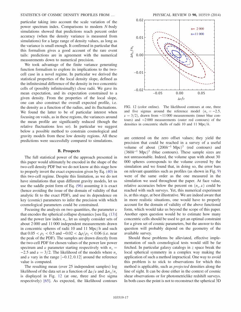
that encodes the spherical collapse dynamics [see Eq. (13)]and the power law index ns, let us simply consider sets ofabout 2 000 and 11 000 independent measurements drawnin concentric spheres of radii 10 and 11 Mpc=h and suchthat 0.05 < ρ1 < 0.5 and −0.02 < Δρ=ρ1 < 0.06 (i.e. nearthe peak of the PDF). The samples are drawn directly fromthe two-cell PDF for chosen values of the power law powerspectrum and ν parameter starting respectively with ns ¼−2.5 and ν ¼ 3=2. The likelihood of the models where nsand ν vary in the range ½−0.12; 0.12� around the referencevalue is computed.The resulting mean (over 25 independent samples) log

likelihood of the data set as a function of Δν=ν and Δns=nsis displayed in Fig. 12 (at one, three and five sigmarespectively) [65]. As expected, the likelihood contours

are centered on the zero offset values; they yield theprecision that could be reached in a survey of a usefulvolume of about ð200h−1 MpcÞ3 (red contours) andð360h−1 MpcÞ3 (blue contours). These sample sizes arenot unreasonable. Indeed, the volume span with about 30000 spheres corresponds to the volume covered by thesimulation and we found that, in doing so, the error barson relevant quantities such as profiles (as shown in Fig. 9)were of the same order as the one measured in thesimulation we used throughout the paper. At face value,relative accuracies below the percent on ðns; νÞ could bereached with such surveys. Yet, this numerical experimentis, at this stage, at best illustrative. We are indeed aware thatin more realistic situations, one would have to properlyaccount for the domain of validity of the above functionalform, which would take us beyond the scope of this paper.Another open question would be to estimate how manyconcentric cells should be used to get an optimal constraintfor a given set of cosmic parameters, but the answer to thisquestion will probably depend on the geometry of theavailable survey.Should these problems be alleviated, effective imple-

mentation of such cosmological tests would still be farfetched. In particular galaxy catalogs in z space break thelocal spherical symmetry in a complex way making theapplication of such a method impractical. One way to avoidthis problem is to stick to observations for which thismethod is applicable, such as projected densities along theline of sight. It can be done either in the context of cosmicshear observations or for photometriclike redshift surveys.In both cases the point is not to reconstruct the spherical 3D

FIG. 12 (color online). The likelihood contours at one, threeand five sigmas around the reference model ðns ¼ −2.5;ν ¼ 3=2Þ, drawn from ∼11 000 measurements (inner blue con-tours) and ∼2 000 measurements (outer red contours) of thedensities in concentric shells of radii 10 and 11 Mpc=h.


103519-17

statistics but the circular two-dimensional statistics forwhich the whole method should be applicable followingearly investigations in [27,28]. The accuracy of the pre-dictions still has to be assessed in this context. Anothermissing piece that can be incorporated is the large distancecorrelation of statistical indicators such as profiles andconstrained profiles. Following [27] it is indeed withinreach of this formalism to compute such quantities. Wewould then have a fully working theory that could beexploited in real data sets.

ACKNOWLEDGMENTS

Wewarmly thank D. Pogosyan for triggering our interestin studying the statistics of void regions. We also thank himfor his many comments. This work is partially supported byGrants No. ANR-12-BS05-0002 and No. ANR-13-BS05-0005 of the French Agence Nationale de la Recherche andby the National Science Foundation under Grant No. NSFPHY11-25915. The simulations were run on the HORIZON

cluster. C. P. thanks KITP and the University of Cambridgefor their hospitality while this work was completed. Weacknowledge support from S. Rouberol for running thecluster for us.

APPENDIX A: RADII DECIMATIONS

The purpose of this appendix is to make sure that theexpression of φðfλgÞ is consistent with variable decima-tion, i.e. we want to make sure that

φðfλ1;…; λngÞ¼ φðfλ1;…; λn; λnþ1 ¼ 0;…; λnþm ¼ 0gÞ; ðA1Þ

where the left-hand side is computed from n cells whereasthe right-hand side is computed with nþm cells.In order to prove this property, let us define a set A of n

cells and a set B of m cells. One can then define thecovariance matrix σijðρi; ρjÞ as in (17) between two anycells of the union of A and B.We first need to establish a preliminary relation between

the element of the inverse matrix ΞijðfρkgÞ and thecovariance matrix. FromXn

l¼1

σilðρi; ρlÞΞljðfρkgÞ ¼ δij; ðA2Þ

we indeed can derive the following relation,

σilðρi; ρlÞ∂∂ρk ½ΞljðfρkgÞ�σjmðρj; ρmÞ

þ ∂∂ρk ½σimðρi; ρmÞ� ¼ 0; ðA3Þ

where all the repeated indices run from 1 to nþm. One canalso write this relation when the inverse matrix is defined

from the covariance matrix of the cells restricted in A only.Let us define by ΞμνðfρρμgÞ this matrix and in the followingrestrict the Greek indices from 1 to n. The previous relationis then transformed into

σμλðρμ; ρλÞ∂∂ρκ ½ΞλνðfρμgÞ�σνσðρν; ρσÞ

þ ∂∂ρκ ½σμσðρμ; ρσÞ� ¼ 0: ðA4Þ

The cumulant generating functions for the n cells in A isgiven by

φðfλμgÞ ¼ λμτμ −1

2Ξμντμτν; ðA5Þ

with the stationary conditions

λκ ¼ Ξμκτμdτκdρκ

þ 1

2

∂Ξμν

∂ρκ τμτν: ðA6Þ

The purpose of the following calculation is to show that it isidentical to the expression of φðλiÞ describing the cumulantgenerating function of the nþm cells when the last m − nvalues of λi are set to zero. In this case we have

φðfλμ; 0gÞ ¼ λμτμ −1

2Ξijτiτj; ðA7Þ

with the stationary conditions

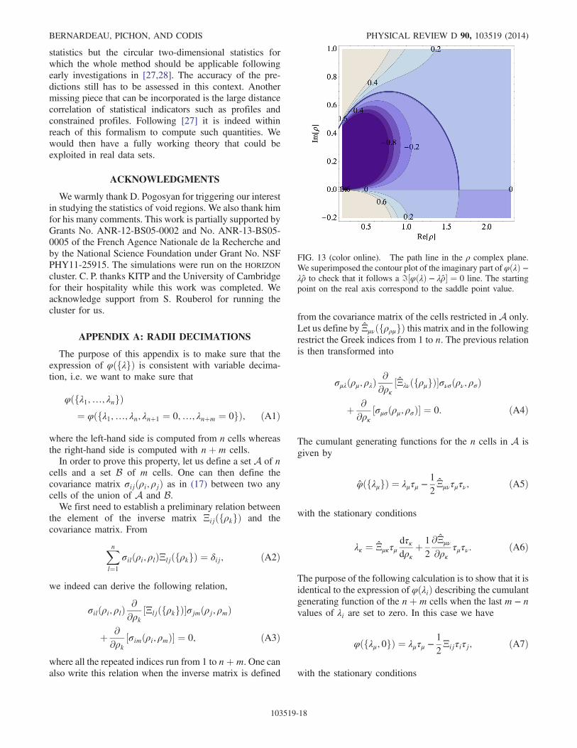
FIG. 13 (color online). The path line in the ρ complex plane.We superimposed the contour plot of the imaginary part of φðλÞ −λρ to check that it follows a ℑ½φðλÞ − λρ� ¼ 0 line. The startingpoint on the real axis correspond to the saddle point value.


103519-18

λκ ¼ Ξiκτidτκdρκ

þ 1

2

∂Ξij

∂ρκ τiτj; ðA8Þ

0 ¼ Ξkiτidτkdρk

þ 1

2

∂Ξij

∂ρk τiτj; ðA9Þ

for k running from nþ 1 to nþm. The second set ofconstraints allows to determine the values of τi for i ∈½nþ 1; nþm� in terms of τν. It is given by

τi ¼ σiμΞμντν; ðA10Þ

where once again repeated Greek indices are summed overfrom 1 to n. This expression is actually valid for any valuesof i as when i is in the 1 to n range we identically haveτi ¼ τi. One can indeed check that for this expressionthe two terms in Eq. (A9) are identically 0: indeed Ξkiτi ¼δkμ ¼ 0 for k ∈ ½nþ 1; nþm� and ∂Ξij=∂ρkτiτj¼∂Ξij=∂ρkσiμΞμντνσjμ0 Ξμ0ν0τν0 ¼−∂σμμ0=∂ρkΞμντνΞμ0ν0τν0 ¼0

for k ∈ ½nþ 1; nþm�. Then replacing using this expres-sion for the τi in Eq. (A8), one gets

λκ ¼ ΞiκσiμΞμντνdτκdρκ

þ 1

2

∂Ξij

∂ρκ σiμΞμντνσjμ0 Ξμ0ν0τν0 :

Its first term can be simplified using the definition of Ξ andthe second by the subsequent use of Eqs. (A3) and (A4),

∂Ξij

∂ρκ σiμΞμνσjμ0 Ξμ0ν0 ¼ −∂∂ρκ σμμ0 ΞμνΞμ0ν0 ;

¼ ∂Ξκσ

∂ρκ σκμΞμνσσμ0 Ξμ0ν0 ;

¼ ∂Ξνν0

∂ρκ ; ðA11Þ

so that the expression of λκ coincides with the expression(A6). Finally τμ ¼ τμ ensures that the property (A1) is valid.

APPENDIX B: INTEGRATIONIN THE COMPLEX PLANE

1. Numerical algorithm

The computation of the one-point PDF relies on thefollowing expression:

PðρÞ ¼Z þi∞

−i∞

dλ2πi

expð−λρþ φðλÞÞ; ðB1Þ

where we explicitly denote ρ as the value of the density forwhich we want to compute the PDF. This is to distinguish itfrom the variable ρ that enters in the calculation of φðλÞ outof the Legendre transform of ΨðρÞ. The idea to achieve fast

convergence of the integral is to follow a path in thecomplex plane where the argument of the exponential inEq. (B1) is real. The starting point of the calculation isρ ¼ ρs. When ρ is small enough (in the regular region) thenwe simply have ρs ¼ ρ otherwise one should take ρs ¼ ρc.At this very location, two lines of vanishing imaginary partsof −λρþ φðλÞ cross, one along the real axis (obviously)and one parallel to the imaginary axis (precisely because weare at a saddle point position). The idea is then to build, stepby step, a path by imposing

δ½φðλÞ − λρ� ∈ R: ðB2Þ

This condition can be written as an infinitesimal variationof λ. Recalling that dφðλÞ=dλ ¼ ρðλÞ, for each step we haveto impose

ðρ − ρÞδλ ∈ R; ðB3Þ

which in turns can be obtained by imposing that thecomplex argument of ðδρÞ is that of ½ðρ − ρÞd2Ψ=dρ2��.This is what we implement in practice. Accurate predictionfor the PDFs are obtained with about 50 points along thepath line that is illustrated on Fig. 13.

2. The large density tails

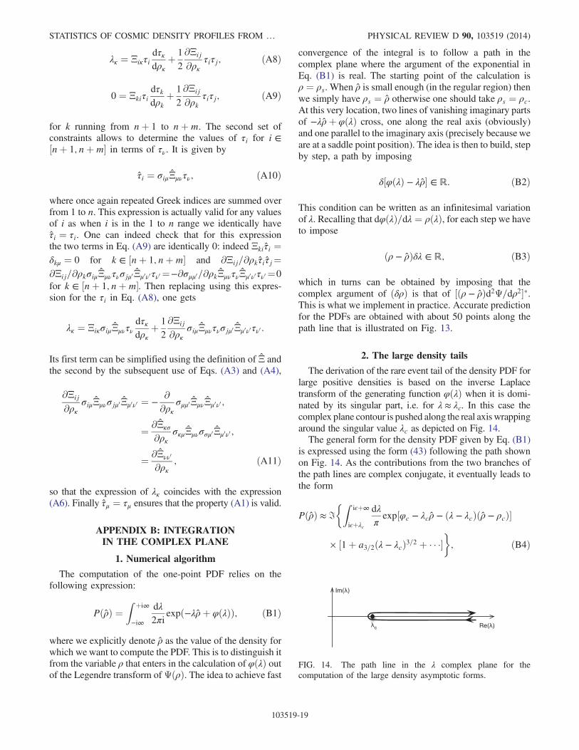
The derivation of the rare event tail of the density PDF forlarge positive densities is based on the inverse Laplacetransform of the generating function φðλÞ when it is domi-nated by its singular part, i.e. for λ ≈ λc. In this case thecomplex plane contour is pushed along the real axis wrappingaround the singular value λc as depicted on Fig. 14.The general form for the density PDF given by Eq. (B1)

is expressed using the form (43) following the path shownon Fig. 14. As the contributions from the two branches ofthe path lines are complex conjugate, it eventually leads tothe form

PðρÞ ≈ ℑ

Ziϵþ∞

iϵþλc

dλπexp½φc − λcρ − ðλ − λcÞðρ − ρcÞ�

× ½1þ a3=2ðλ − λcÞ3=2 þ � � ��; ðB4Þ

FIG. 14. The path line in the λ complex plane for thecomputation of the large density asymptotic forms.


103519-19

where we keep only the dominant singular part in φðλÞ andwhere ℑ denotes the imaginary part. This integral can easilybe computed and it leads to

PðρÞ ≈ exp ðφc − λcρÞ�

3ℑða32Þ

4ffiffiffiπ

p ðρ − ρcÞ5=2þ � � �

�: ðB5Þ

Subleading contributions can be computed in a similar waywhen expðφðλÞÞ is expanded to higher order. Note that bysymmetry, only half integer terms that appear in thisexpansion will actually contribute.

APPENDIX C: THE CONSTRAINEDVARIANCE

In this appendix we complement the calculations startedin Sec. IV E where we computed the expected slope under alocal density constraint. Pursuing along the same line ofcalculations, the variance of ρ2 given ρ1 can be computedfrom the conditional value of ρ22. It is given by the secondderivative of the moment generating function, and istherefore given byZ

dρ2ρ22Pðρ1; ρ2Þ

¼Z þi∞

−i∞

dλ12πi

�∂2φðλ1; λ2Þ∂λ22

λ2¼0

þ�∂φðλ1; λ2Þ

∂λ2 λ2¼0

�2�expð−λ1ρ1 þ φðλ1ÞÞ:

The calculation of its approximate form in the low-ρ saddlepoint limit is a bit more cumbersome. Indeed, in the lowvariance limit in which this approximation is derived thetwo terms in the square brackets are not of the same order,the first being subdominant with respect the second. It isnonetheless possible to compute the resulting cumulant inthe low density limit. Formally, differentiating Eq. (90)with respect to λ2 we have

∂2φðλ1; λ2Þ∂λ22 ¼ ∂ρ2ðλ1; λ2Þ

∂λ2 ; ðC1Þ

from the Legendre stationary condition, which, afterinversion of the partial derivatives, is formally given by

∂2φðλ1; λ2Þ∂λ22 ¼ Ψ;ρ1ρ1

Ψ;ρ1ρ1Ψ;ρ2ρ2 −Ψ2;ρ1ρ2

; ðC2Þ

where Ψ;ρiρj ≡ ∂2Ψ=∂ρi∂ρj are calculated at the station-ary point. On the other hand ∂φðλ1; λ2Þ=∂λ2 can beexpanded as

∂φðλ1; λ2Þ∂λ2 ¼ φðλs; 0Þ þ ðλ1 − λsÞ

×∂2φðλ1; λ2Þ∂λ2∂λ1 þ 1

2ðλ1 − λsÞ2

∂3φðλ1; λ2Þ∂λ2∂λ21 þ � � �

ðC3Þ

near the saddle point value λs. The integration of∂φðλ1; λ2Þ=∂λ2 in the complex plane therefore leads toa correction from the ðλ1 − λsÞ2 term. It can be verifiedthough that this contribution vanishes when one takesthe cumulant. The integration of ð∂φðλ1; λ2Þ=∂λ2Þhowever leads to an extra term due to the second termin the previous expansion. The resulting term reads½∂2φ=∂λ2∂λ1�2=∂2φ=∂λ21, so that

hρ22iρ1 − hρ2i2ρ1 ¼∂2φ

∂λ21 −� ∂2φ

∂λ2∂λ1�2

=∂2φ

∂λ21¼

�∂2φ

∂λ21∂2φ

∂λ22 −� ∂2φ

∂λ1∂λ2�

2�=∂2φ

∂λ21 ; ðC4Þ

which can be rewritten more compactly as

hρ22iρ1 − hρ2i2ρ1 ¼ 1=Ψ;ρ2ρ2 jρ1;ρ2ðρ1Þ; ðC5Þ

when expressed in terms of Ψ.

APPENDIX D: SIMULATIONS

For the purpose of this paper, we have carried out adark matter simulation with GADGET2 [66]. This simulationis characterized by the following ΛCDM cosmology:Ωm ¼ 0.265, ΩΛ ¼ 0.735, n ¼ 0.958, H0 ¼ 70 km ×s−1 ×Mpc−1 and σ8 ¼ 0.8, Ωb ¼ 0.045 within one stan-dard deviation of Wilkinson Microwave Anisotropy Probe7 results [67]. The box size is 500 Mpc=h sampled with10243 particles, the softening length 24 kpc=h. Initialconditions are generated using MPGRAFIC [68]. The var-iances and running indexes are measured from the theo-retical power spectra produced by MPGRAFIC. Snapshots aresaved for z ¼ 0; 0.65; 0.97; 1.46; 2.33 and 3.9. An Octree isbuilt for each snapshot, which allows us to count veryefficiently all particles within a given sequence of concen-tric spheres of radii between R ¼ 4; 5… up to 18 Mpc=h.The center of these spheres is sampled regularly on a grid of10 Mpc=h aside, leading to 117 649 estimates of thedensity per snapshot. All histograms drawn in this paperare derived from these samples. Note that the cells overlapfor radii larger than 10 Mpc=h.

APPENDIX E: SYSTEMATIC COMPARISONSWITH SIMULATION

We collect here figures that are too large to be put in themain text.


103519-20

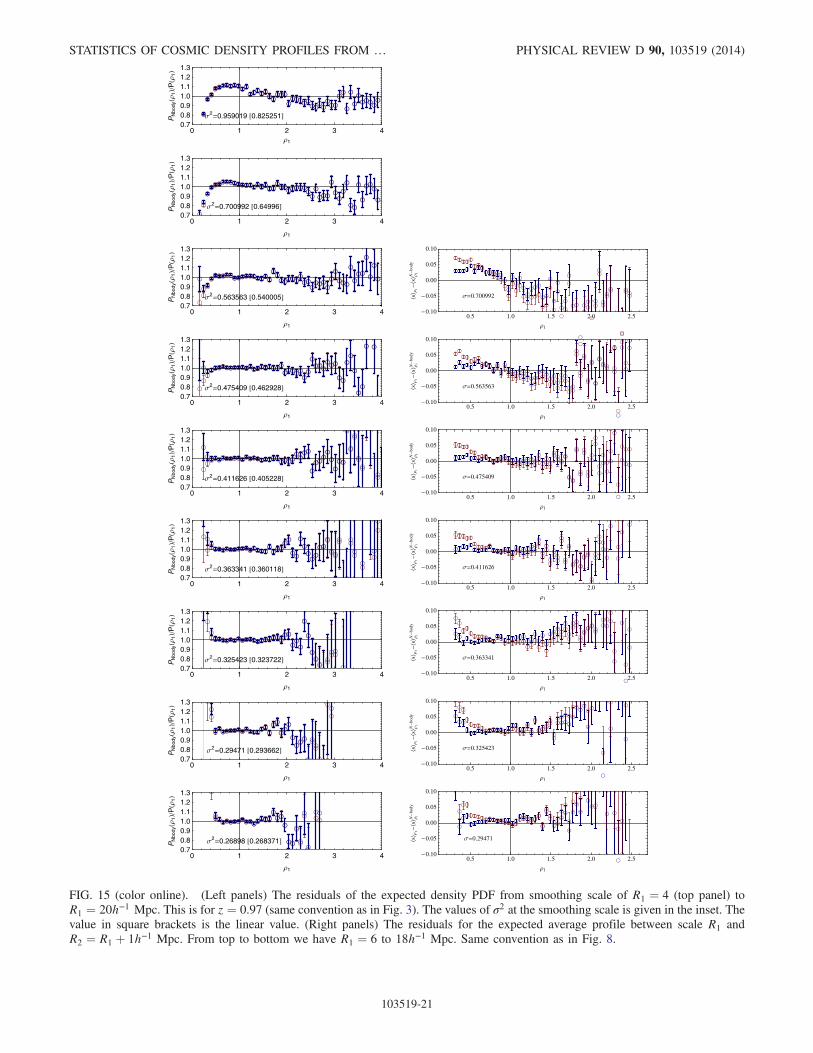
0 1 2 3 40.70.80.91.01.11.21.3

1

PN

body

1P

1

2 0.959019 0.825251

0 1 2 3 40.70.80.91.01.11.21.3

1

PN

body

1P

1

2 0.700992 0.64996

0 1 2 3 40.70.80.91.01.11.21.3

1

PN

body

1P

1

2 0.563563 0.540005

0 1 2 3 40.70.80.91.01.11.21.3

1

PN

body

1P

1

2 0.475409 0.462928

0 1 2 3 40.70.80.91.01.11.21.3

1

PN

body

1P

1

2 0.411626 0.405228

0 1 2 3 40.70.80.91.01.11.21.3

1

PN

body

1P

1

2 0.363341 0.360118

0 1 2 3 40.70.80.91.01.11.21.3

1

PN

body

1P

1

2 0.325423 0.323722

0 1 2 3 40.70.80.91.01.11.21.3

1

PN

body

1P

1

2 0.29471 0.293662

0 1 2 3 40.70.80.91.01.11.21.3

1

PN

body

1P

1

2 0.26898 0.268371

0.5 1.0 1.5 2.0 2.50.10

0.05

0.00

0.05

0.10

1

s1

s1

Nbo

dy

0.700992

0.5 1.0 1.5 2.0 2.50.10

0.05

0.00

0.05

0.10

1s

1s

1

Nbo

dy

0.563563

0.5 1.0 1.5 2.0 2.50.10

0.05

0.00

0.05

0.10

1

s1

s1

Nbo

dy

0.475409

0.5 1.0 1.5 2.0 2.50.10

0.05

0.00

0.05

0.10

1

s1

s1

Nbo

dy

0.411626

0.5 1.0 1.5 2.0 2.50.10

0.05

0.00

0.05

0.10

1

s1

s1

Nbo

dy

0.363341

0.5 1.0 1.5 2.0 2.50.10

0.05

0.00

0.05

0.10

1

s1

s1

Nbo

dy

0.325423

0.5 1.0 1.5 2.0 2.50.10

0.05

0.00

0.05

0.10

1

ss

1

Nbo

dy

0.29471

FIG. 15 (color online). (Left panels) The residuals of the expected density PDF from smoothing scale of R1 ¼ 4 (top panel) toR1 ¼ 20h−1 Mpc. This is for z ¼ 0.97 (same convention as in Fig. 3). The values of σ2 at the smoothing scale is given in the inset. Thevalue in square brackets is the linear value. (Right panels) The residuals for the expected average profile between scale R1 andR2 ¼ R1 þ 1h−1 Mpc. From top to bottom we have R1 ¼ 6 to 18h−1 Mpc. Same convention as in Fig. 8.


103519-21

[1] See http://bigboss.lbl.gov, https://www.darkenergysurvey.org, http://pan-starrs.ifa.hawaii.edu, and http://www.lsst.org.

[2] R. Laureijs, J. Amiaux, S. Arduini, J.-L. Auguères,J. Brinchmann, R. Cole, M. Cropper, C. Dabin, L. Duvet,A. Ealet et al., arXiv:1110.3193.

[3] See http://sci.esa.int/euclid, http://snap.lbl.gov, and http://jdem.lbl.gov.

[4] S. F. Daniel, E. V. Linder, T. L. Smith, R. R. Caldwell,A. Cooray, A. Leauthaud, and L. Lombriser, Phys. Rev.D 81, 123508 (2010).

[5] A. F. Heavens, T. D. Kitching, and L. Verde, Mon. Not. R.Astron. Soc. 380, 1029 (2007).

[6] F. Bernardeau, S. Colombi, E. Gaztañaga, and R.Scoccimarro, Phys. Rep. 367, 1 (2002).

[7] M. Crocce and R. Scoccimarro, Phys. Rev. D 73, 063519(2006).

[8] A. Taruya and T. Hiramatsu, Astrophys. J. 674, 617 (2008).[9] M. Pietroni, J. Cosmol. Astropart. Phys. 10 (2008) 036.

[10] M. Crocce, R. Scoccimarro, and F. Bernardeau, Mon. Not.R. Astron. Soc. 427, 2537 (2012).

[11] A. Taruya, F. Bernardeau, T. Nishimichi, and S. Codis,Phys. Rev. D 86, 103528 (2012).

[12] J. J. M. Carrasco, M. P. Hertzberg, and L. Senatore, J. HighEnergy Phys. 09 (2012) 082.

[13] J. M. Bardeen, J. R. Bond, N. Kaiser, and A. S. Szalay,Astrophys. J. 304, 15 (1986).

[14] J. R. Gott III, Publ. Astron. Soc. Pac. 100, 1307 (1988).[15] K. R. Mecke, T. Buchert, and H. Wagner, Astron.

Astrophys. 288, 697 (1994).[16] S. Colombi, D. Pogosyan, and T. Souradeep, Phys. Rev.

Lett. 85, 5515 (2000).[17] C. Gay, C. Pichon, and D. Pogosyan, Phys. Rev. D 85,

023011 (2012).[18] T. Matsubara, Astrophys. J. Lett. 434, L43 (1994).[19] S. Codis, C. Pichon, D. Pogosyan, F. Bernardeau, and

T. Matsubara, Mon. Not. R. Astron. Soc. 435, 531 (2013).[20] R. Balian and R. Schaeffer, Astron. Astrophys. 220, 1

(1989).[21] F. Bernardeau, Astrophys. J. 392, 1 (1992).[22] F. Bernardeau, Astron. Astrophys. 291, 697 (1994).[23] R. Juszkiewicz, F. R. Bouchet, and S. Colombi, Astrophys.

J. Lett. 412, L9 (1993).[24] F. Bernardeau, Astrophys. J. 433, 1 (1994).[25] C. M. Baugh, E. Gaztanaga, and G. Efstathiou, Mon. Not.

R. Astron. Soc. 274, 1049 (1995).[26] F. Bernardeau, Astron. Astrophys. 312, 11 (1996).[27] F. Bernardeau, Astron. Astrophys. 301, 309 (1995).[28] F. Bernardeau and P. Valageas, Astron. Astrophys. 364, 1

(2000).[29] P. Valageas, Astron. Astrophys. 382, 412 (2002).[30] G. Lavaux and B. D. Wandelt, Astrophys. J. 754, 109

(2012).[31] P. M. Sutter, G. Lavaux, B. D. Wandelt, and D. H. Weinberg,

Astrophys. J. 761, 44 (2012).[32] K. Bolejko and R. A. Sussman, Phys. Lett. B 697, 265

(2011).[33] R. van de Weygaert and E. Platen, Int. J. Mod. Phys. Conf.

Ser. 01, 41 (2011).

[34] M. A. Aragon-Calvo, R. van de Weygaert, P. A. Araya-Melo, E. Platen, and A. S. Szalay, Mon. Not. R. Astron. Soc.404, L89 (2010).

[35] G. Lavaux and B. D. Wandelt, Mon. Not. R. Astron. Soc.403, 1392 (2010).

[36] M. A. Aragon-Calvo and A. S. Szalay, Mon. Not. R. Astron.Soc. 428, 3409 (2013).

[37] Specifically, we expect perturbation theory to break downlater in low density regions; we also expect these regions toprobe smaller Lagrangian scales.

[38] J. Binney, N. Dowrick, A. Fisher, and M. Newman,The Theory of Critical Phenomena (Oxford University,New York, 1992).

[39] C. Heyde, J. R. Stat. Soc. Ser. B 25, 392 (1963).[40] It is to be noted however that it is not necessarily defined

for any real values of λ as one expects for instance that theone-point density PDF develops an exponential cutoff,PðρÞ ∼ expð−λcρÞ, which implies that φðλÞ is undefinedwhen λ > λc.

[41] This comes from a simple counting of lines: one needs atleast p − 1 lines to connect p points which in turns forcesthe sum of orders at which each factor is computed to be2ðp − 1Þ; see [6,21,22,42].

[42] J. N. Fry, Astrophys. J. 279, 499 (1984).[43] P. J. E. Peebles, The Large-Scale Structure of the Universe,

Princeton Series in Physics, edited by S. B. Treiman(Princeton University, Princeton, NJ, 1980).

[44] F. Bernardeau, Cosmologie: Des Fondements Théoriquesaux Observations (EDP Sciences, Les Ulis, France, 2007).

[45] We could choose ν ¼ 3=2 in order to reproduce the lowdensity asymptotic behavior of the exact solution.

[46] We implicitly assume throughout this paper that the initialconditions are adiabatic so that the perturbations developedout of a single scalar field degree of freedom.

[47] This is actually a superfluous hypothesis but we adopt it forconvenience. Transient effects form mildly non-Gaussianinitial conditions can for instance be taken into account inthis formalism as shown in [48].

[48] P. Valageas, Astron. Astrophys. 382, 431 (2002).[49] This relation is a priori time dependent but we will omit it in

the following.[50] This inversion is possible as long as ΨðfτkgÞ is a convex

function of ρk which in practice means before shell crossing.[51] Thus, if we define φinitðfλkgÞ as the cumulant generating

function of the density contrasts at initial time, we haveΨinitðfρkgÞ ¼

Piρiλi − φinitðfλkgÞ, with ρi ¼ ∂φinit=∂λi. It

is easy to check that for Gaussian initial conditions,φinitðfλigÞ ¼

Piλi þ 1

2

PijΣijλiλj, which leads to the

expression (25) given previously for Ψ.[52] F. Bernardeau and R. Schaeffer, Astron. Astrophys. 255, 1

(1992).[53] It is beyond the scope of this paper to discuss the validity of

this inversion and how it can generally be implemented.Interested readers can find detailed discussions of thisconstruction in [20] in the context of cosmological densityPDF and counts in cells statistics, where it has been carriedout in particular for the one-point PDF, the properties ofwhich are crucially related to the analytical properties of thecumulant generating function.


103519-22

http://bigboss.lbl.gov



https://www.darkenergysurvey.org

https://www.darkenergysurvey.org

http://pan-starrs.ifa.hawaii.edu

http://www.lsst.org

http://www.lsst.org

http://arXiv.org/abs/1110.3193

http://sci.esa.int/euclid



http://snap.lbl.gov

http://jdem.lbl.gov

http://jdem.lbl.gov



http://dx.doi.org/10.1111/j.1365-2966.2007.12134.x

http://dx.doi.org/10.1111/j.1365-2966.2007.12134.x

http://dx.doi.org/10.1016/S0370-1573(02)00135-7



http://dx.doi.org/10.1086/526515

http://dx.doi.org/10.1088/1475-7516/2008/10/036

http://dx.doi.org/10.1111/j.1365-2966.2012.22127.x

http://dx.doi.org/10.1111/j.1365-2966.2012.22127.x


http://dx.doi.org/10.1007/JHEP09(2012)082

http://dx.doi.org/10.1007/JHEP09(2012)082

http://dx.doi.org/10.1086/164143

http://dx.doi.org/10.1103/PhysRevLett.85.5515

http://dx.doi.org/10.1103/PhysRevLett.85.5515



http://dx.doi.org/10.1086/187570

http://dx.doi.org/10.1093/mnras/stt1316

http://dx.doi.org/10.1086/171398

http://dx.doi.org/10.1086/186927

http://dx.doi.org/10.1086/186927

http://dx.doi.org/10.1086/174620

http://dx.doi.org/10.1051/0004-6361:20011663

http://dx.doi.org/10.1088/0004-637X/754/2/109

http://dx.doi.org/10.1088/0004-637X/754/2/109

http://dx.doi.org/10.1088/0004-637X/761/1/44

http://dx.doi.org/10.1016/j.physletb.2011.02.007

http://dx.doi.org/10.1016/j.physletb.2011.02.007

http://dx.doi.org/10.1142/S2010194511000092

http://dx.doi.org/10.1142/S2010194511000092

http://dx.doi.org/10.1111/j.1745-3933.2010.00841.x

http://dx.doi.org/10.1111/j.1745-3933.2010.00841.x

http://dx.doi.org/10.1111/j.1365-2966.2010.16197.x

http://dx.doi.org/10.1111/j.1365-2966.2010.16197.x

http://dx.doi.org/10.1093/mnras/sts281

http://dx.doi.org/10.1093/mnras/sts281

http://dx.doi.org/10.1086/161913

http://dx.doi.org/10.1051/0004-6361:20011675

[54] In [52] this inversion was initially performed for models ofnonlinear clustering (hierarchical models) taking advantageof the general results presented in [20]. The same techniqueswere later employed in the context of perturbation theorycalculations. For all these constructions, the analyticalproperties of the cumulant generating function follow fromthe structure of the stationary condition.

[55] Note that in practice π3 is negative and that only thenonregular parts appearing in the expansion of expðφðλÞÞwill contribute.

[56] The change of sign in Eq. (45) comes from the path that isorthogonal to the real axis.

[57] F. Bernardeau, Astrophys. J. Lett. 390, L61 (1992).[58] An alternative approach would be to use predicted ampli-

tude form direct next-to-leading-order perturbation theorycalculations. We leave this option for further studies.

[59] F. Bernardeau and L. Kofman, Astrophys. J. 443, 479(1995).

[60] The difference can be, to a large extent, interpreted by thenonlinear growth of the reduced skewness.

[61] In practice this is achieved via a series expansion inversionof Eq. (24) then plugged in Eq. (23).

[62] Again when ns is less than −1 in case of a power lawspectrum.

[63] The location of the resulting critical line is only weaklysensitive to the threshold we choose.

[64] It involves expressing P as a function of φ, expressing ρ2integrating over ρ2 and using Cauchy’s theorem.

[65] A similar experiment for three-cells of size R ¼ 11; 12 and13 Mpc=h was carried out, producing similar results.

[66] V. Springel, Mon. Not. R. Astron. Soc. 364, 1105 (2005).[67] E. Komatsu, K. M. Smith, J. Dunkley, C. L. Bennett, B.

Gold, G. Hinshaw, N. Jarosik, D. Larson, M. R. Nolta, L.Page et al., Astrophys. J. Suppl. Ser. 192, 18 (2011).

[68] S. Prunet, C. Pichon, D. Aubert, D. Pogosyan, R. Teyssier,and S. Gottloeber, Astophys. J. Suppl. Ser. 178, 179 (2008).


103519-23

http://dx.doi.org/10.1086/186372

http://dx.doi.org/10.1086/175542

http://dx.doi.org/10.1086/175542

http://dx.doi.org/10.1111/j.1365-2966.2005.09655.x

http://dx.doi.org/10.1088/0067-0049/192/2/18

http://dx.doi.org/10.1086/590370

Documents

Statistics of cosmic density profiles from perturbation theory